Advanced Structural Econometrics: Dynamic Games, Auctions & HANK

Solvers, Simulation, Equilibrium Computation & Estimation

Athanassios Stavrakoudis

astavrak@uoi.gr

Applied Informatics and Computational Economics Lab

11 July 2026

Required Packages

library(tidyverse)   # dplyr for wrangling, ggplot2 for every figure
# Base R supplies optim(), solve() and the linear algebra used throughout;
# each later Part loads the one specialised package it needs, where it needs it.

import numpy as np                 # arrays, linear algebra, random draws
import pandas as pd                # tabular data
import matplotlib.pyplot as plt    # figures
from scipy import optimize, stats  # optimisers and distributions

* Base Stata plus Mata cover the solvers and simulations in the foundations.
* Domain commands are introduced Part-by-Part, where they are first used.

About This Deck

• Part I — Foundations: what makes a model structural, and the computational objects that recur — fixed points, simulation, high-dimensional state
• Parts II–IV — Dynamic games: Markov-perfect equilibrium, its estimation (NFXP vs CCP), and the modern frontier
• Parts V–VI — Auctions: private- and common-value models, identification from bids, the modern toolkit
• Parts VII–VIII — HANK: heterogeneous-agent macro — solving and estimating models with a whole distribution as a state
• Parts IX–X — Unifying themes and three worked case studies
• Every computational slide runs in , and ; all computation is inline — no black box hides the algorithm

The Computational Angle

• Three Recurring Objects
• The Payoff

What ties dynamic games, auctions and HANK together is less their economics than their computation. Three objects recur in all three:

• Fixed points — an equilibrium solves \(x = \Gamma(x)\): a Bellman operator, a best-response map, a market-clearing price, a distribution that reproduces itself
• Simulation — when a moment or likelihood has no closed form we simulate it, and the estimator inherits Monte-Carlo error shrinking like \(1/\sqrt{S}\)
• High-dimensional state — adding players, or a wealth distribution, explodes the state space: the curse of dimensionality

The reason to solve these hard objects is the counterfactual: primitives estimated in one environment let us re-solve behaviour in an environment never observed.

 Two loops, not one

Structural estimation almost always nests two numerical problems. The inner solver takes a candidate parameter () and returns the model’s predicted behaviour (()) — a fixed point. The outer estimator searches over () to make that predicted behaviour match the data.

The solver runs once per candidate (), so the outer search may call it thousands of times:

[ = _ Q(, ()). ]

Almost every trick in this course — CCP two-step methods, the sequence-space Jacobian, machine-learning surrogates — is a way to make the inner solve cheaper or avoidable. Keep the two loops separate in your mind and the whole field organises itself.

Literature Review

• Ericson, R., & Pakes, A. (1995). Markov-perfect industry dynamics. Review of Economic Studies, 62(1), 53–82. DOI: 10.2307/2297841
• Aguirregabiria, V., & Mira, P. (2007). Sequential estimation of dynamic discrete games. Econometrica, 75(1), 1–53. DOI: 10.1111/j.1468-0262.2007.00731.x
• Bajari, P., Benkard, C. L., & Levin, J. (2007). Estimating dynamic models of imperfect competition. Econometrica, 75(5), 1331–1370. DOI: 10.1111/j.1468-0262.2007.00796.x
• Guerre, E., Perrigne, I., & Vuong, Q. (2000). Optimal nonparametric estimation of first-price auctions. Econometrica, 68(3), 525–574. DOI: 10.1111/1468-0262.00123
• Athey, S., & Haile, P. A. (2002). Identification of standard auction models. Econometrica, 70(6), 2107–2140. DOI: 10.1111/1468-0262.00371
• Kaplan, G., Moll, B., & Violante, G. L. (2018). Monetary policy according to HANK. American Economic Review, 108(3), 697–743. DOI: 10.1257/aer.20160042
• Auclert, A., Bardóczy, B., Rognlie, M., & Straub, L. (2021). Using the sequence-space Jacobian to solve and estimate heterogeneous-agent models. Econometrica, 89(5), 2375–2408. DOI: 10.3982/ECTA17434
• Achdou, Y., Han, J., Lasry, J.-M., Lions, P.-L., & Moll, B. (2022). Income and wealth distribution in macroeconomics: a continuous-time approach. Review of Economic Studies, 89(1), 45–86. DOI: 10.1093/restud/rdab002
• Judd, K. L. (1998). Numerical Methods in Economics. MIT Press. ISBN 9780262100717

Part I — Foundations of Structural Econometrics

Primitives, equilibrium, and the computation that ties the field together

What Is Structural Econometrics?

• Model = Primitives + Equilibrium
• The Structural Bargain

A structural model writes the data as the output of an economic mechanism, not as a correlation among observables. It has three parts:

• Primitives \(\theta\) — preferences, technology, information, the distribution of shocks: the objects that do not move when policy does
• An equilibrium concept — optimisation plus a consistency condition (best responses, market clearing) mapping primitives to behaviour
• A solution — the policies, bids, prices or choice probabilities the model predicts, which are then confronted with data

\[ \underbrace{\theta}_{\text{primitives}} \;\xrightarrow{\;\text{equilibrium } \sigma(\theta)\;}\; \underbrace{P_\theta(\text{behaviour})}_{\text{model prediction}} \]

Estimation inverts this arrow: find the \(\theta\) whose predicted behaviour best matches the observed data.

The reason to pay the price of a full model is the counterfactual: because \(\theta\) is policy-invariant, we can change the environment, re-solve \(\sigma(\theta)\), and predict behaviour in a world never seen in the data.

 What makes a parameter “structural”?

A reduced-form coefficient answers “how do observables co-move?” It is a property of the data-generating distribution under the current regime. Change the policy and it can change too.

A structural parameter — a taste, a cost, a discount factor — is a property of the agents themselves. It is assumed invariant to the policy, which is exactly what licences the counterfactual.

Concretely, a decision rule (a = g(x;,)) is not structural: it mixes the primitive with the environment. The primitive () that generates (g) through optimisation is. Recovering () and re-deriving (g) under a new policy is the entire game.

Why Structural? Counterfactuals from Primitives

• The Point

A reduced-form regression tells us what happened; only a model of the primitives tells us what would happen under a policy never tried. The smallest possible example: a monopolist with known demand \(p = a - bq\) and marginal cost \(c\).

\[ \max_{q}\ (a - bq - c)\,q \;\;\Rightarrow\;\; q^\star(c) = \frac{a - c}{2b},\qquad p^\star(c) = \frac{a + c}{2} \]

• We never observe the world with a tax — but the primitives \((a,b,c)\) let us re-solve the firm’s problem with \(c \to c + \tau\)
• Welfare accounting: \(W = \underbrace{\tfrac12 b\,q^2}_{\text{consumer surplus}} + \text{profit} + \underbrace{\tau q}_{\text{tax revenue}}\); the drop is the deadweight loss
• No estimation here — just the Solve and Counterfactual steps, to show what structure buys

a <- 10; b <- 1; mc <- 2      # inverse demand p = a - b q ; marginal cost mc
tax <- 1                       # counterfactual: a per-unit tax

solve_monopoly <- function(cost) {
  q <- (a - cost) / (2 * b)
  p <- a - b * q
  c(q = q, p = p, cs = 0.5 * b * q^2, profit = (p - cost) * q)
}
base <- solve_monopoly(mc)          # the world we observe
cf   <- solve_monopoly(mc + tax)    # re-solved under the tax
taxrev <- tax * cf["q"]
W_base <- base["cs"] + base["profit"]
W_cf   <- cf["cs"]  + cf["profit"] + taxrev

             price  quantity     CS   profit  tax rev

baseline      6.00     4.00    8.00   16.00      --

tax = 1       6.50     3.50    6.12   12.25    3.50

total welfare  24.000  ->  21.875     deadweight loss = 2.125

a, b, mc, tax = 10.0, 1.0, 2.0, 1.0

def solve_monopoly(cost):
    q = (a - cost) / (2 * b)
    p = a - b * q
    return q, p, 0.5 * b * q**2, (p - cost) * q

qb, pb, csb, prb = solve_monopoly(mc)         # observed world
qc, pc, csc, prc = solve_monopoly(mc + tax)   # re-solved under the tax
taxrev = tax * qc
Wb, Wc = csb + prb, csc + prc + taxrev

print("             price  quantity     CS   profit  tax rev")

             price  quantity     CS   profit  tax rev

print(f"baseline    {pb:6.2f}   {qb:6.2f}  {csb:6.2f}  {prb:6.2f}      --")

baseline      6.00     4.00    8.00   16.00      --

print(f"tax = 1     {pc:6.2f}   {qc:6.2f}  {csc:6.2f}  {prc:6.2f}  {taxrev:6.2f}")

tax = 1       6.50     3.50    6.12   12.25    3.50

print(f"total welfare  {Wb:.3f}  ->  {Wc:.3f}     deadweight loss = {Wb-Wc:.3f}")

total welfare  24.000  ->  21.875     deadweight loss = 2.125

mata:
a = 10; b = 1; mc = 2; tax = 1
qb = (a-mc)/(2*b);        pb = a - b*qb
csb = 0.5*b*qb^2;         prb = (pb-mc)*qb
qc = (a-(mc+tax))/(2*b);  pc = a - b*qc
csc = 0.5*b*qc^2;         prc = (pc-(mc+tax))*qc
taxrev = tax*qc
Wb = csb + prb
Wc = csc + prc + taxrev
printf("             price  quantity     CS   profit  tax rev\n")
printf("baseline    %6.2f   %6.2f  %6.2f  %6.2f      --\n", pb, qb, csb, prb)
printf("tax = 1     %6.2f   %6.2f  %6.2f  %6.2f  %6.2f\n", pc, qc, csc, prc, taxrev)
printf("total welfare  %6.3f  ->  %6.3f     deadweight loss = %6.3f\n", Wb, Wc, Wb-Wc)
end

------------------------------------------------- mata (type end to exit) ----------------------------------------------
: a = 10; b = 1; mc = 2; tax = 1

: qb = (a-mc)/(2*b);        pb = a - b*qb

: csb = 0.5*b*qb^2;         prb = (pb-mc)*qb

: qc = (a-(mc+tax))/(2*b);  pc = a - b*qc

: csc = 0.5*b*qc^2;         prc = (pc-(mc+tax))*qc

: taxrev = tax*qc

: Wb = csb + prb

: Wc = csc + prc + taxrev

: printf("             price  quantity     CS   profit  tax rev\n")
             price  quantity     CS   profit  tax rev

: printf("baseline    %6.2f   %6.2f  %6.2f  %6.2f      --\n", pb, qb, csb, prb)
baseline      6.00     4.00    8.00   16.00      --

: printf("tax = 1     %6.2f   %6.2f  %6.2f  %6.2f  %6.2f\n", pc, qc, csc, prc, taxrev)
tax = 1       6.50     3.50    6.12   12.25    3.50

: printf("total welfare  %6.3f  ->  %6.3f     deadweight loss = %6.3f\n", Wb, Wc, Wb-Wc)
total welfare  24.000  ->  21.875     deadweight loss =  2.125

: end
------------------------------------------------------------------------------------------------------------------------

The Classical Workflow

• Five Stages
• The Nested Loop

• Specify — write the primitives \(\theta\) and the equilibrium concept
• Solve — given \(\theta\), compute the equilibrium behaviour \(\sigma(\theta)\) (a fixed point)
• Estimate — invert: find \(\hat\theta\) so predicted behaviour matches the data
• Validate — fit, out-of-sample checks, over-identifying restrictions
• Counterfactual — change the environment, re-solve, predict

The expensive step is Solve: it usually sits inside the estimation loop, run once per candidate \(\theta\). Nearly the whole computational literature is about making that inner solve affordable.

\[ \hat\theta = \arg\min_\theta\ Q\big(\text{data},\ \sigma(\theta)\big), \qquad \sigma(\theta)\ \text{re-solved at every } \theta \]

If the outer optimiser evaluates \(Q\) a thousand times, the model is solved a thousand times — each solve itself an iteration to a fixed point. That is why a millisecond per solve and a minute per solve are different research projects.

 Three ways to cheapen the loop

The recurring trick of the field is to avoid re-solving the model at every parameter guess:

• Two-step / CCP methods (Hotz–Miller): read the policy straight off the data, so the inner fixed point is solved once, not per (). Part III.
• Sequence-space / linearisation (Auclert et al.): solve the model once at a point and reuse its Jacobian for estimation. Part VIII.
• Surrogates: train a fast approximation to (()) — a neural net or interpolant — and query it inside the loop. Parts IV and VIII.

Every one of them trades a little statistical efficiency for a large computational saving.

Identification Challenges

• What Can the Data Pin Down?

Identification asks whether the data could ever distinguish two parameter vectors, before any noise. It is a property of the model and the observables — not of the sample size. A model can fit perfectly and still leave \(\theta\) set-identified, not point-identified.

• Functional form — flexible primitives can trace the same behaviour many ways
• Equilibrium selection — with multiple equilibria the map \(\theta \to\) data is a correspondence (Parts II, IV)
• Dynamics — the discount factor is notoriously weakly identified from choices alone

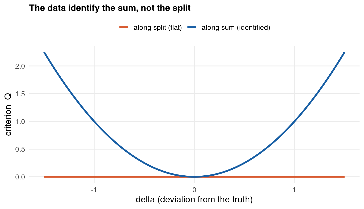
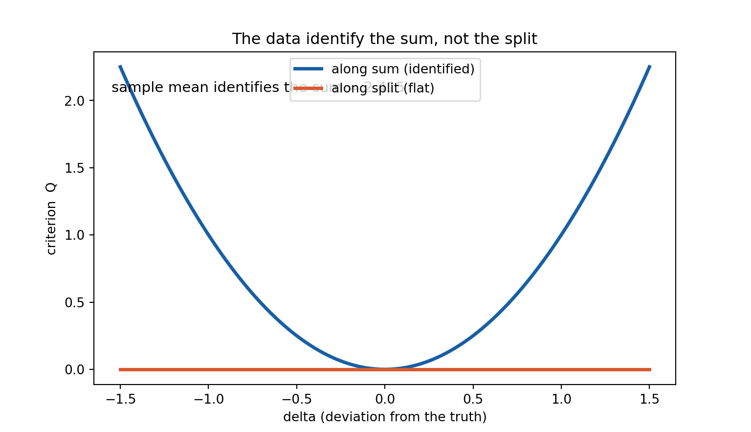
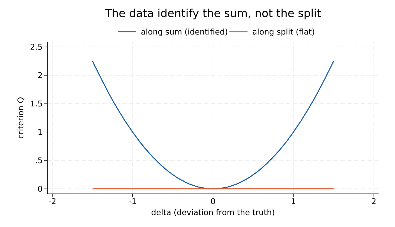
A minimal caricature: suppose the data reveal only the sum \(\theta_1 + \theta_2\) (through a sample mean). Moving along the sum is visible; moving along the split \(\theta_1 - \theta_2\) is invisible.

ident <- read.csv("../data/gah-identification.csv")  # from advanced-structural-data.R
ybar  <- mean(ident$y)                                # data pin down the SUM = mean
delta <- seq(-1.5, 1.5, length.out = 121)             # deviation from the truth
Q_sum   <- delta^2                 # move theta1+theta2: criterion rises
Q_split <- rep(0, length(delta))   # move theta1-theta2: criterion unchanged

prof <- data.frame(delta = rep(delta, 2), Q = c(Q_sum, Q_split),
  dir = rep(c("along sum (identified)", "along split (flat)"), each = length(delta)))
ggplot(prof, aes(delta, Q, colour = dir)) +
  geom_line(linewidth = 1.3) +
  scale_colour_manual(values = c("along sum (identified)" = "#185FA5",
                                 "along split (flat)" = "#D85A30")) +
  labs(x = "delta (deviation from the truth)", y = "criterion  Q", colour = NULL,
       title = "The data identify the sum, not the split") +
  theme_lecture + theme(legend.position = "top")

Sample mean identifies the sum theta1+theta2 = 2.415

Moving the split leaves the criterion at 0 -- the split is not identified

import numpy as np, pandas as pd
import matplotlib.pyplot as plt

ident = pd.read_csv("../data/gah-identification.csv")   # same file as R
ybar = ident["y"].mean()
delta = np.linspace(-1.5, 1.5, 121)
Q_sum = delta**2
Q_split = np.zeros_like(delta)

# number goes on the figure: a Python plot chunk drops its stdout under knitr
fig, ax = plt.subplots(figsize=(8, 4.6))
ax.plot(delta, Q_sum, color="#185FA5", lw=2.6, label="along sum (identified)")
ax.plot(delta, Q_split, color="#D85A30", lw=2.6, label="along split (flat)")
ax.text(0.03, 0.88, f"sample mean identifies the sum = {ybar:.3f}",
        transform=ax.transAxes, fontsize=11)
_ = ax.set(xlabel="delta (deviation from the truth)", ylabel="criterion  Q",
           title="The data identify the sum, not the split")
ax.legend(loc="upper center")
plt.show()

quietly import delimited "../data/gah-identification.csv", clear
quietly summarize y
display "Sample mean identifies the sum theta1+theta2 = " %5.3f r(mean)
mata:
delta  = rangen(-1.5, 1.5, 121)
Qsum   = delta:^2
Qsplit = J(rows(delta), 1, 0)
st_matrix("PROF", (delta, Qsum, Qsplit))
end
clear
quietly set obs 121
quietly svmat double PROF, names(v)
rename (v1 v2 v3) (delta qsum qsplit)
quietly twoway (line qsum delta, lcolor("24 95 165") lwidth(medthick)) ///
  (line qsplit delta, lcolor("216 90 48") lwidth(medthick)), ///
  xtitle("delta (deviation from the truth)") ytitle("criterion Q") ///
  title("The data identify the sum, not the split") ///
  legend(order(1 "along sum (identified)" 2 "along split (flat)") pos(12) rows(1))
quietly graph export "../plots/gah-identification.png", replace width(1600)

Sample mean identifies the sum theta1+theta2 = 2.415

------------------------------------------------- mata (type end to exit) ----------------------------------------------
: delta  = rangen(-1.5, 1.5, 121)

: Qsum   = delta:^2

: Qsplit = J(rows(delta), 1, 0)

: st_matrix("PROF", (delta, Qsum, Qsplit))

: end
------------------------------------------------------------------------------------------------------------------------

Estimation Methods — Four Lenses

• The Toolkit
• Coincide, Then Diverge

Four paradigms recur through the deck; each matches the model to data differently:

• MLE — maximise the likelihood \(\prod_i f(w_i;\theta)\). Efficient when the density is known and tractable
• GMM — match theoretical to sample moments: robust, needs no full distribution, over-identification is testable
• SMM / Indirect Inference — when moments have no closed form, simulate them; pay a \(1/\sqrt{S}\) price in variance
• Bayesian — put a prior on \(\theta\) and compute the posterior; natural for high-dimensional or weakly-identified models

On a textbook model the four often agree. Their differences appear exactly in the settings this deck is about:

• with over-identification, GMM’s \(J\)-test and MLE part ways
• with an intractable likelihood (dynamic games, HANK), only simulation-based or Bayesian methods run at all
• with weak identification (discount factors, flat ridges), the prior does real work

 A rough map

• Dynamic games (Parts II–IV): MLE via nested fixed point when feasible; CCP / two-step GMM when not.
• Auctions (Parts V–VI): nonparametric identification then GMM or MLE on the recovered value distribution.
• HANK (Parts VII–VIII): simulated method of moments and Bayesian estimation, because the likelihood is a functional of a distribution.

The lesson is not “pick one” but “the model chooses for you”: tractability of the likelihood and the strength of identification decide which lens is even available.

Computational Bottlenecks

• Equilibrium = Fixed Point

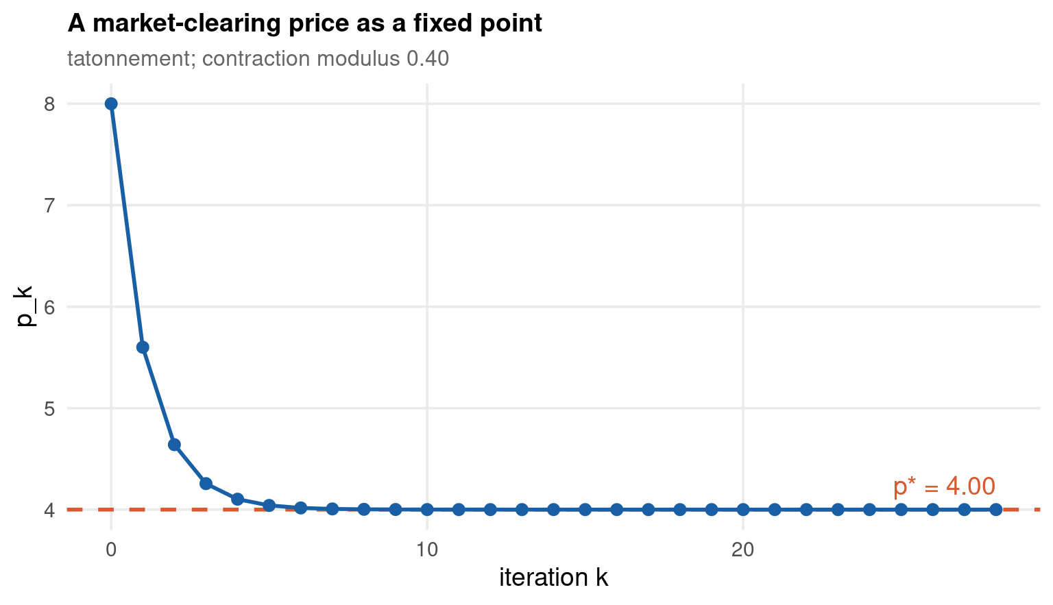
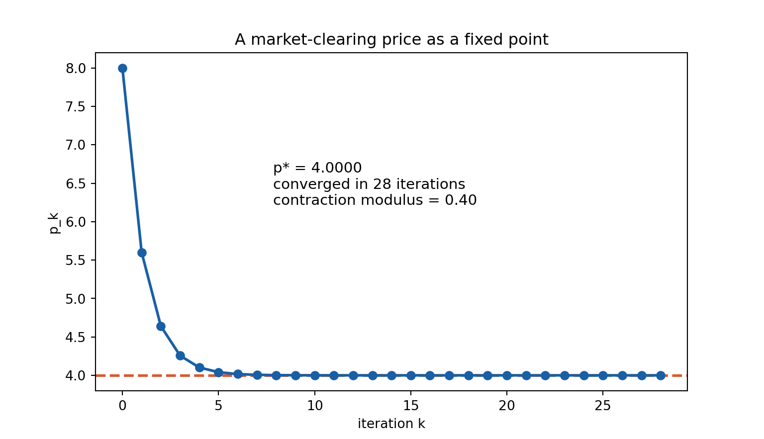
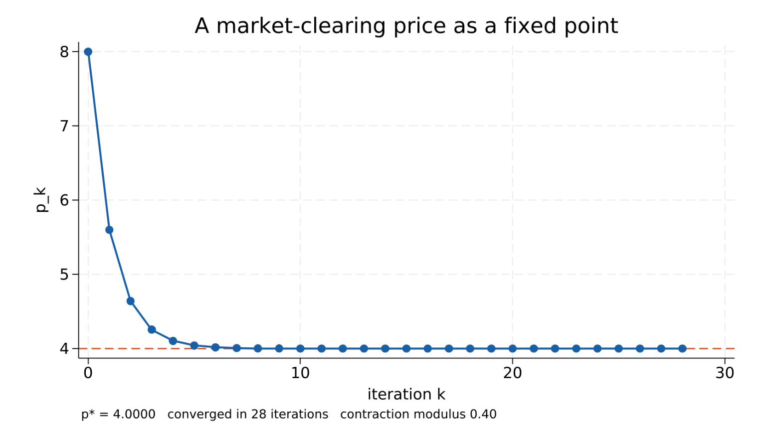
Every equilibrium in this course is a solution to \(x = \Gamma(x)\). When \(\Gamma\) is a contraction — \(\lVert \Gamma(x) - \Gamma(y)\rVert \le L\lVert x - y\rVert\) with \(L < 1\) — simple iteration converges geometrically from any start.

The canonical example that recurs in games and in HANK is a market that clears: demand \(a - bp\), supply \(c + dp\), price nudged by excess demand.

\[ p_{k+1} = \Gamma(p_k) = p_k + \eta\big[(a - b p_k) - (c + d p_k)\big], \qquad p^\star = \frac{a - c}{b + d} \]

• The modulus is \(\lvert 1 - \eta(b+d)\rvert\); smaller means faster convergence
• The other two bottlenecks — simulation error (\(\propto 1/\sqrt{S}\)) and the curse of dimensionality — return in Parts III and II respectively

a <- 10; b <- 1; cc <- 2; d <- 1     # demand a - b p ; supply cc + d p
eta <- 0.3                            # tatonnement speed
pstar <- (a - cc) / (b + d)           # equilibrium we are solving for
p <- 8; path <- p                     # start away from equilibrium
repeat {
  excess <- (a - b*p) - (cc + d*p)    # excess demand
  p_new  <- p + eta * excess          # p_{k+1} = Gamma(p_k)
  path   <- c(path, p_new)
  if (abs(p_new - p) < 1e-10) break
  p <- p_new
}
iters <- length(path) - 1
rate  <- abs(1 - eta*(b + d))         # contraction modulus

ggplot(data.frame(k = 0:iters, p = path), aes(k, p)) +
  geom_hline(yintercept = pstar, linetype = "dashed", colour = "#D85A30", linewidth = 1) +
  geom_line(colour = "#185FA5", linewidth = 1) +
  geom_point(colour = "#185FA5", size = 2.5) +
  labs(x = "iteration k", y = "p_k",
       title = "A market-clearing price as a fixed point") +
  theme_lecture

Equilibrium price p* = 4.0000   (solved as a fixed point)

Converged in 28 iterations; contraction modulus = 0.40

import numpy as np
import matplotlib.pyplot as plt

a, b, cc, d, eta = 10.0, 1.0, 2.0, 1.0, 0.3
pstar = (a - cc) / (b + d)
p, path = 8.0, [8.0]
while True:
    excess = (a - b*p) - (cc + d*p)   # excess demand
    p_new = p + eta*excess            # p_{k+1} = Gamma(p_k)
    path.append(p_new)
    if abs(p_new - p) < 1e-10:
        break
    p = p_new
iters = len(path) - 1
rate = abs(1 - eta*(b + d))

# numbers go on the figure: a Python plot chunk drops its stdout under knitr
fig, ax = plt.subplots(figsize=(8, 4.6))
ax.axhline(pstar, ls="--", color="#D85A30", lw=2)
ax.plot(range(iters + 1), path, color="#185FA5", lw=2, marker="o", markersize=6)
ax.text(0.30, 0.55,
        f"p* = {pstar:.4f}\nconverged in {iters} iterations\ncontraction modulus = {rate:.2f}",
        transform=ax.transAxes, fontsize=11)
_ = ax.set(xlabel="iteration k", ylabel="p_k",
           title="A market-clearing price as a fixed point")
plt.show()

mata:
a = 10; b = 1; cc = 2; d = 1; eta = 0.3
pstar = (a - cc)/(b + d)
p = 8; path = p; diff = 1
while (diff > 1e-10) {
  excess = (a - b*p) - (cc + d*p)     // excess demand
  pnew = p + eta*excess               // p_{k+1} = Gamma(p_k)
  path = (path \ pnew)
  diff = abs(pnew - p)
  p = pnew
}
iters = rows(path) - 1
rate  = abs(1 - eta*(b + d))
st_matrix("FP", ((0::iters), path))
st_numscalar("pstar", pstar)
st_numscalar("iters", iters)
st_numscalar("rate", rate)
end
* numbers travel on the plot (Statamarkdown drops console text after a Mata
* block in a plot chunk), so p*, iterations and modulus go in the note()
local ps : display %5.4f pstar
local rt : display %4.2f rate
local it = iters
clear
quietly set obs `=rowsof(FP)'
quietly svmat double FP, names(v)
rename (v1 v2) (k p)
quietly twoway (line p k, lcolor("24 95 165") lwidth(medthick)) ///
  (scatter p k, mcolor("24 95 165") msize(medium)), ///
  yline(`=scalar(pstar)', lpattern(dash) lcolor("216 90 48")) ///
  xtitle("iteration k") ytitle("p_k") legend(off) ///
  title("A market-clearing price as a fixed point") ///
  note("p* = `ps'   converged in `it' iterations   contraction modulus `rt'")
quietly graph export "../plots/gah-fixedpoint.png", replace width(1600)

Part II — Dynamic Games: Classical Theory

Static vs Dynamic Games

Markov Perfect Equilibrium (MPE)

Ericson–Pakes (1995)

State Transitions

Equilibrium Existence & Multiplicity

Computational Methods

Curse of Dimensionality

Part III — Dynamic Games: Estimation

Two Estimation Paradigms

NFXP (Rust 1987)

CCP (Hotz–Miller)

Aguirregabiria–Mira (2002, 2007)

Identification in Dynamic Games

Computational Tricks

Applications

Part IV — Modern Dynamic Games

Dynamic Oligopoly with Learning

Dynamic Auctions as Games

Dynamic Pricing Games

Dynamic Matching & Search Models

Dynamic Games with Networks

Recent Literature

Computational Advances

Part V — Auctions: Classical Structural Models

Why Auctions?

Private-Value Auctions

Common-Value Auctions

Revenue Equivalence

Bid Functions & Equilibrium

Identification

Estimation Approaches

Empirical Applications

Part VI — Modern Auction Econometrics

Auctions with Asymmetric Bidders

Auctions with Risk Aversion

Dynamic Auctions

Common-Value Auctions & Winner’s Curse

Bidder Collusion Detection

Machine Learning in Auctions

Recent Literature

Part VII — Heterogeneous-Agent Macro (HANK): Foundations

From RANK to HANK

Why Heterogeneity Matters

Household Problem

Firm Problem

Market Clearing & Aggregation

Equilibrium Definition

Computational Methods

Part VIII — HANK: Estimation & Modern Literature

Solving HANK Models

Estimation Approaches

HANK + Monetary Policy

HANK + Fiscal Policy

HANK + Labor Markets

Recent Literature

Computational Innovations

Part IX — Unified Themes Across Dynamic Games, Auctions & HANK

Dynamic Programming Everywhere

Equilibrium Selection Problems

Simulation-Based Estimation

Computational Constraints

Modern Solutions

Part X — Case Studies

Case Study 1: Airline Entry Game

Case Study 2: Spectrum Auction

Case Study 3: Monetary Policy in HANK