Bayesian and Hierarchical Panels in Econometrics

Partial Pooling, Shrinkage & Multilevel Models for Panel Data
using , &

Athanassios Stavrakoudis

astavrak@uoi.gr

Applied Informatics and Computational Economics Lab

5 July 2026

Required Packages

library(tidyverse)    # data wrangling and ggplot2
library(brms)         # Bayesian multilevel models via Stan (NUTS)
library(rstan)        # the Stan engine brms compiles to
library(bayesplot)    # trace plots, rank plots, posterior predictive checks
library(loo)          # LOO-CV / WAIC model comparison
library(coda)         # classical MCMC diagnostics
library(lme4)         # lmer() — frequentist multilevel benchmark
library(plm)          # within / random-effects panel estimators

import numpy as np
import pandas as pd
import matplotlib.pyplot as plt
import pymc as pm                    # NUTS sampler, PyMC >= 5
import arviz as az                   # posterior diagnostics and plots
import statsmodels.api as sm
from linearmodels import PanelOLS, RandomEffects

* Everything used here is built-in Stata (16+):
*   bayes: mixed        Bayesian multilevel / hierarchical models
*   bayesstats summary  posterior summaries
*   bayesgraph          trace / density / autocorrelation diagnostics
*   mixed, xtreg        frequentist benchmarks
* No ssc installs required for this deck.

About This Deck

• Part I: Foundations — why panel heterogeneity is a Bayesian problem; the pooling spectrum and shrinkage
• Part II: A known-truth laboratory — a simulated hierarchical panel where every parameter is known
• Part III: Estimation — the same random-intercept, random-slope model in brms, PyMC and bayes: mixed; recovering the truth; shrinkage in action
• Part IV: Priors, convergence & model checking — variance-component priors, R-hat/ESS, posterior predictive checks, LOO/WAIC
• Part V: Real data I — random-coefficient investment equations on the Grunfeld firm panel
• Part VI: Real data II — the union wage premium in the Vella–Verbeek panel; Bayesian vs frequentist FE/RE
• Part VII: Bayesian testing — posterior probabilities, Savage–Dickey ratios, ROPE
• All computational slides run in , and ; R generates every shared dataset (bayesian-hp-data.R)

Literature Review

• Lindley, D. V., & Smith, A. F. M. (1972). Bayes estimates for the linear model. JRSS Series B, 34(1), 1–41. DOI: 10.1111/j.2517-6161.1972.tb00885.x
• Swamy, P. A. V. B. (1970). Efficient inference in a random coefficient regression model. Econometrica, 38(2), 311–323. DOI: 10.2307/1913012
• Mundlak, Y. (1978). On the pooling of time series and cross section data. Econometrica, 46(1), 69–85. DOI: 10.2307/1913646
• Gelman, A., & Hill, J. (2007). Data Analysis Using Regression and Multilevel/Hierarchical Models. Cambridge University Press. DOI: 10.1017/CBO9780511790942
• Gelman, A. (2006). Prior distributions for variance parameters in hierarchical models. Bayesian Analysis, 1(3), 515–534. DOI: 10.1214/06-BA117A
• Rossi, P. E., Allenby, G. M., & McCulloch, R. (2005). Bayesian Statistics and Marketing. Wiley. DOI: 10.1002/0470863692
• Vella, F., & Verbeek, M. (1998). Whose wages do unions raise? A dynamic model of unionism and wage rate determination for young men. Journal of Applied Econometrics, 13(2), 163–183. DOI: 10.1002/(SICI)1099-1255(199803/04)13:2<163::AID-JAE460>3.0.CO;2-Y
• Kleiber, C., & Zeileis, A. (2010). The Grunfeld data at 50. German Economic Review, 11(4), 404–417. DOI: 10.1111/j.1468-0475.2010.00513.x
• Bürkner, P.-C. (2017). brms: An R package for Bayesian multilevel models using Stan. Journal of Statistical Software, 80(1), 1–28. DOI: 10.18637/jss.v080.i01
• Salvatier, J., Wiecki, T. V., & Fonnesbeck, C. (2016). Probabilistic programming in Python using PyMC3. PeerJ Computer Science, 2, e55. DOI: 10.7717/peerj-cs.55
• Vehtari, A., Gelman, A., & Gabry, J. (2017). Practical Bayesian model evaluation using leave-one-out cross-validation and WAIC. Statistics and Computing, 27, 1413–1432. DOI: 10.1007/s11222-016-9696-4
• Betancourt, M., & Girolami, M. (2015). Hamiltonian Monte Carlo for hierarchical models. arXiv: 1312.0906

Part I: Foundations

Why panel heterogeneity is a Bayesian problem

The Problem & Motivation

• The Panel Problem
• The Frequentist Dilemma
• The Bayesian Answer

A panel follows \(N\) units (firms, workers, countries) over \(T\) periods:

\[ y_{it} = \alpha_i + \beta_i\, x_{it} + \varepsilon_{it}, \qquad i = 1, \dots, N, \quad t = 1, \dots, T \]

• Units are heterogeneous: each firm has its own baseline \(\alpha_i\) and possibly its own response \(\beta_i\)
• \(T\) is usually small (5–20 periods) — each unit gives only a handful of observations
• The core question of panel econometrics: how much should unit \(i\) borrow from the other units?

Classical panel econometrics forces a corner solution:

• Pooled OLS — pretend \(\alpha_i = \alpha\) for all \(i\): biased if heterogeneity is real
• Fixed effects — estimate every \(\alpha_i\) separately: unbiased, but each \(\hat\alpha_i\) uses only \(T\) observations, so it is noisy; time-invariant covariates drop out
• Random effects — assume \(\alpha_i \perp x_{it}\): efficient, but inconsistent when the assumption fails (Hausman test)
• Unit-by-unit OLS for \(\beta_i\) with \(T = 10\)? Standard errors so wide the estimates are nearly useless

Each choice is all-or-nothing: pool completely, or not at all.

Treat the unit-specific parameters as draws from a population distribution:

\[ \alpha_i \sim \mathcal{N}(\mu_\alpha, \tau_\alpha^2), \qquad \beta_i \sim \mathcal{N}(\mu_\beta, \tau_\beta^2) \]

• The data decide how much to pool: if units look alike (\(\tau\) small), estimates are pulled together; if they differ (\(\tau\) large), each unit keeps its own estimate
• Partial pooling is a continuum between pooled OLS and fixed effects — chosen by the likelihood, not by the researcher
• Full posterior distributions for every quantity: unit effects, hyperparameters, predictions
• Works even when some units have very few observations — they simply borrow more strength

Bayes Refresher — From Prior to Hierarchy

• Bayes’ Rule
• Adding a Hierarchy
• Exchangeability

For parameters \(\theta\) and data \(y\), all inference flows from the posterior:

\[ p(\theta \mid y) \;=\; \frac{p(y \mid \theta)\, p(\theta)}{p(y)} \;\propto\; \underbrace{p(y \mid \theta)}_{\text{likelihood}} \times \underbrace{p(\theta)}_{\text{prior}} \]

• The posterior is a full distribution, not a point estimate — credible intervals, tail probabilities and predictions all come from it directly
• Modern samplers (Hamiltonian Monte Carlo / NUTS) draw from \(p(\theta \mid y)\) even when it has thousands of dimensions — exactly what a panel with \(N\) unit effects requires

A hierarchical (multilevel) model stacks priors in levels:

\[ \text{Level 1 (data):} \quad y_{it} \mid \alpha_i, \beta_i \;\sim\; \mathcal{N}\!\left(\alpha_i + \beta_i x_{it},\; \sigma^2\right) \]

\[ \text{Level 2 (units):} \quad \alpha_i \sim \mathcal{N}(\mu_\alpha, \tau_\alpha^2), \qquad \beta_i \sim \mathcal{N}(\mu_\beta, \tau_\beta^2) \]

\[ \text{Level 3 (hyperpriors):} \quad \mu_\alpha, \mu_\beta \sim \mathcal{N}(0, 5^2), \qquad \tau_\alpha, \tau_\beta, \sigma \sim \mathcal{N}^{+}(0, 2^2) \]

• Level 2 is the population distribution of unit effects — its parameters \((\mu, \tau)\) are estimated, not assumed
• The idea dates to Lindley & Smith (1972) and, in econometrics, to Swamy’s (1970) random-coefficients model

When is the hierarchy justified? When units are exchangeable: before seeing the data, no unit is special — the joint distribution of \((\alpha_1, \dots, \alpha_N)\) is invariant to relabelling.

• By de Finetti’s theorem, exchangeable effects behave as if drawn iid from some common distribution — precisely the Level-2 assumption
• Exchangeability fails when a unit is known a priori to differ (e.g. one country in a currency union, one giant firm) — then add covariates at Level 2 or group units
• Note the parallel with random effects: RE assumes \(\alpha_i \perp x_{it}\); the Bayesian hierarchy makes the same assumption unless we model the correlation (Mundlak device — see Variations)

“Bayesian random effects” does not fix endogeneity

The hierarchical prior \(\alpha_i \sim \mathcal{N}(\mu_\alpha, \tau_\alpha^2)\) plays the same structural role as the frequentist random-effects assumption. If the unit effects are correlated with the regressors, the posterior for \(\mu_\beta\) is centred on the wrong value, no matter how well the chains mix. Bayesians handle this the same way Mundlak (1978) did: include the unit means \(\bar{x}_i\) as a Level-2 covariate, turning the model into a correlated-random-effects specification.

The Pooling Spectrum

• Three Estimators
• The Shrinkage Weight
• Why It Wins

For the unit intercepts \(\alpha_i\) (with \(\bar{y}_i\) the unit mean), the three classical answers are:

\[ \hat\alpha_i^{\text{complete pool}} = \bar{y} \qquad\qquad \hat\alpha_i^{\text{no pool}} = \bar{y}_i \]

\[ \hat\alpha_i^{\text{partial pool}} \;=\; w_i\, \bar{y}_i \;+\; (1 - w_i)\, \mu_\alpha \]

• Complete pooling: one number for everyone — ignores heterogeneity
• No pooling: fixed effects — ignores similarity
• Partial pooling: a precision-weighted compromise — the hierarchical posterior mean

The pooling weight is determined by the two variance components:

\[ w_i \;=\; \frac{\tau_\alpha^2}{\tau_\alpha^2 + \sigma^2 / T_i} \]

• \(\tau_\alpha^2\) large (units genuinely differ) \(\Rightarrow\) \(w_i \to 1\): trust the unit’s own data — approaches fixed effects
• \(\tau_\alpha^2\) small (units alike) \(\Rightarrow\) \(w_i \to 0\): pool towards \(\mu_\alpha\) — approaches pooled OLS
• \(T_i\) large \(\Rightarrow\) \(w_i \to 1\): with enough own data, no borrowing is needed
• Crucially, \(\tau_\alpha\) and \(\sigma\) are estimated from the data — the data choose the position on the spectrum

• Efficiency: partial pooling dominates no pooling in mean-squared error whenever the hierarchy holds — the multilevel generalisation of the James–Stein result
• Small groups: units with tiny \(T_i\) get stabilised instead of producing wild estimates
• Prediction for new units: the population distribution \(\mathcal{N}(\mu_\alpha, \tau_\alpha^2)\) is the forecast for a unit never seen before — fixed effects has no answer here

Shrinkage trades a little bias for a lot of variance

Yes, the partial-pooling estimate of any single \(\alpha_i\) is biased towards \(\mu_\alpha\). But its variance is so much smaller than the no-pooling estimate’s that the mean squared error across all units falls — often dramatically when \(T\) is small. In the known-truth laboratory of Part III you will see this: the shrunken estimates sit closer to the true \(\beta_i\) than the unit-by-unit OLS estimates they were shrunk from.

Methodology — The Hierarchical Linear Panel Model

• Full Model
• Hyperpriors
• Non-Centered Parameterisation
• Computation

The workhorse of this deck — varying intercepts and varying slopes with correlation:

\[ y_{it} = \alpha_i + \beta_i\, x_{it} + \varepsilon_{it}, \qquad \varepsilon_{it} \sim \mathcal{N}(0, \sigma^2) \]

\[ \begin{pmatrix} \alpha_i \\ \beta_i \end{pmatrix} \sim \mathcal{N}\!\left( \begin{pmatrix} \mu_\alpha \\ \mu_\beta \end{pmatrix},\; \boldsymbol{\Sigma} \right), \qquad \boldsymbol{\Sigma} = \mathbf{D}\, \boldsymbol{\Omega}\, \mathbf{D}, \quad \mathbf{D} = \text{diag}(\tau_\alpha, \tau_\beta) \]

• \(\boldsymbol{\Omega}\) is the \(2 \times 2\) correlation matrix of the unit effects — units with high baselines may respond differently
• Frequentist twin: lmer(y ~ x + (1 + x | id)) — same likelihood, no hyperpriors, REML point estimates

\[ \mu_\alpha, \mu_\beta \sim \mathcal{N}(0, 5^2), \qquad \tau_\alpha, \tau_\beta \sim \mathcal{N}^{+}(0, 2^2), \qquad \sigma \sim \mathcal{N}^{+}(0, 2^2), \qquad \boldsymbol{\Omega} \sim \text{LKJ}(2) \]

• Half-normal priors on scales are weakly informative: they rule out absurd values but let the data speak (Gelman 2006)
• LKJ(2) gently favours moderate correlations over \(\pm 1\) (Lewandowski, Kurowicka & Joe 2009)
• The old default \(\text{InvGamma}(\epsilon, \epsilon)\) on \(\tau^2\) is a trap: with few units it piles mass near zero and forces over-pooling

With small \(\tau\), samplers stall in the “funnel” of the centered parameterisation. The fix — sample standardised effects and rescale:

\[ z_i \sim \mathcal{N}(0, 1), \qquad \alpha_i = \mu_\alpha + \tau_\alpha\, z_i \]

• The posterior geometry becomes nearly independent of \(\tau_\alpha\) — no funnel, no divergences
• brms and bayes: mixed do this internally; in PyMC we write it explicitly (you will see za, zb in the code)
• Reference: Betancourt & Girolami (2015)

• All three engines use MCMC; R and Python use Hamiltonian Monte Carlo / NUTS, which follows the posterior’s gradient — the method of choice for hierarchies with hundreds of parameters
• Stata’s bayes: mixed uses adaptive Metropolis–Hastings with Gibbs updates for variance components
• We run 2 chains with modest draw counts so slides render quickly; for research use 4 chains and 2,000+ post-warmup draws each
• Every fit is checked with \(\widehat{R}\), effective sample size and posterior predictive checks (Part IV)

Part II: A Known-Truth Laboratory

A simulated hierarchical panel where every parameter is known

DGP — Mathematical Specification

• The Model
• What the Estimators Must Recover
• Why Simulate First

A balanced panel of \(N = 40\) units observed for \(T = 10\) periods:

\[ y_{it} = \alpha_i + \beta_i\, x_{it} + \varepsilon_{it}, \qquad x_{it} \sim \mathcal{N}(0, 1), \qquad \varepsilon_{it} \sim \mathcal{N}(0, 1) \]

\[ \alpha_i \sim \mathcal{N}(2.0,\; 0.8^2), \qquad \beta_i \sim \mathcal{N}(1.5,\; 0.5^2) \]

Because we generate the data, we know every quantity real data hides: the population means \((\mu_\alpha, \mu_\beta) = (2.0, 1.5)\), the heterogeneity scales \((\tau_\alpha, \tau_\beta) = (0.8, 0.5)\), the noise \(\sigma = 1\), and each unit’s individual \((\alpha_i, \beta_i)\).

Parameter	True value	Role
\(\mu_\alpha\)	2.0	population mean intercept
\(\mu_\beta\)	1.5	population mean slope
\(\tau_\alpha\)	0.8	between-unit SD of intercepts
\(\tau_\beta\)	0.5	between-unit SD of slopes
\(\sigma\)	1.0	idiosyncratic noise SD

• With only \(T = 10\) observations per unit, unit-by-unit OLS slopes have \(\text{SE} \approx 1/\sqrt{10} \approx 0.32\) — noisier than the true heterogeneity \(\tau_\beta = 0.5\) they try to measure
• This is exactly the regime where partial pooling pays

• Real panels never reveal whether shrinkage helped — a simulated panel with stored true \((\alpha_i, \beta_i)\) does
• We can compare no pooling vs partial pooling against the truth, unit by unit
• Same discipline as any Monte Carlo study: verify the tools on known ground before touching real data (Parts V–VI)

DGP — Code Implementation

# Full script: bayesian-hp-data.R (creates all shared datasets for this deck)
set.seed(14159)
N <- 40
T_len <- 10
alpha_i <- rnorm(N, mean = 2.0, sd = 0.8)
beta_i  <- rnorm(N, mean = 1.5, sd = 0.5)

sim <- data.frame()
for (i in 1:N) {
  x <- rnorm(T_len)
  y <- alpha_i[i] + beta_i[i] * x + rnorm(T_len, sd = 1)
  sim <- rbind(sim, data.frame(id = i, t = 1:T_len, x = x, y = y))
}
write.csv(sim, "../data/bayes-hp-sim.csv", row.names = FALSE)

truth <- data.frame(id = 1:N, alpha_true = alpha_i, beta_true = beta_i)
write.csv(truth, "../data/bayes-hp-sim-truth.csv", row.names = FALSE)

Wrote ../data/bayes-hp-sim.csv       : 400 rows

Wrote ../data/bayes-hp-sim-truth.csv : 40 rows

Sample moments of the true unit effects:

  mean(alpha_i) = 2.024   sd(alpha_i) = 0.764

  mean(beta_i)  = 1.554   sd(beta_i)  = 0.433

  id t          x          y
1  1 1 -0.3772990  1.9302405
2  1 2 -0.3999774  2.8976870
3  1 3 -0.9804264 -1.3598365
4  1 4  0.8865424  2.9882610
5  1 5 -0.9528133  0.6517793

import pandas as pd

sim = pd.read_csv("../data/bayes-hp-sim.csv")     # always reads R's CSV
truth = pd.read_csv("../data/bayes-hp-sim-truth.csv")
print(sim.head())

   id  t         x         y
0   1  1 -0.377299  1.930240
1   1  2 -0.399977  2.897687
2   1  3 -0.980426 -1.359837
3   1  4  0.886542  2.988261
4   1  5 -0.952813  0.651779

print(f"\nunits: {sim['id'].nunique()}   periods: {sim['t'].nunique()}   rows: {len(sim)}")

units: 40   periods: 10   rows: 400

print(f"true effects stored for {len(truth)} units")

true effects stored for 40 units

import delimited "../data/bayes-hp-sim.csv", clear
quietly destring _all, replace
xtset id t
xtsum y x

(encoding automatically selected: ISO-8859-1)
(4 vars, 400 obs)



Panel variable: id (strongly balanced)
 Time variable: t, 1 to 10
         Delta: 1 unit


Variable         |      Mean   Std. dev.       Min        Max |    Observations
-----------------+--------------------------------------------+----------------
y        overall |  1.752178   1.987413  -3.813023   7.160384 |     N =     400
         between |             .9107732  -.2584071   3.808481 |     n =      40
         within  |             1.771727  -2.611013    7.37585 |     T =      10
                 |                                            |
x        overall | -.0914653   1.017296  -3.112968   2.972849 |     N =     400
         between |             .3382568  -.8498171   1.009444 |     n =      40
         within  |             .9607573  -3.097251   2.539685 |     T =      10

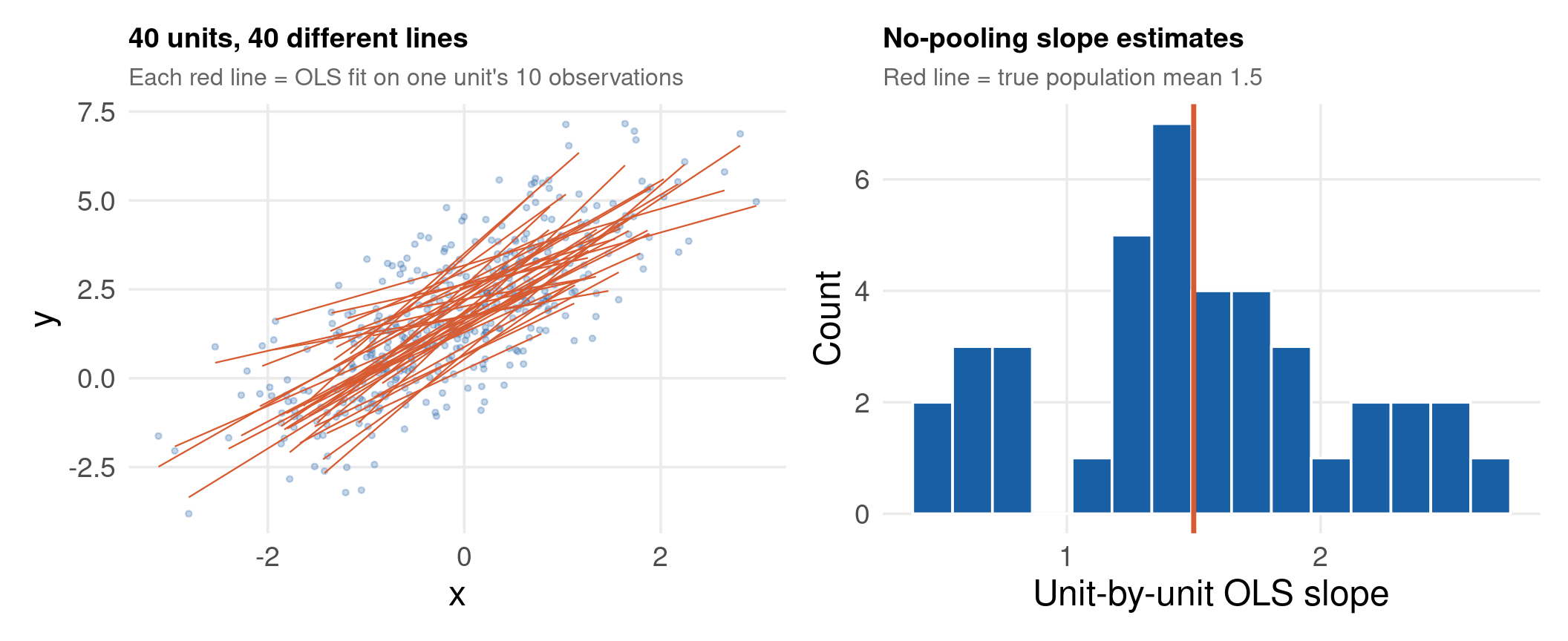
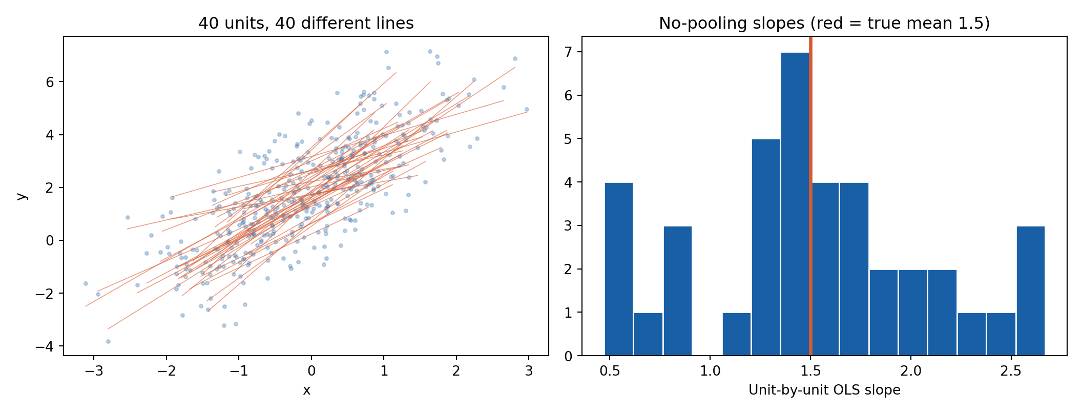
DGP Diagnostics — Seeing the Heterogeneity

sim <- read.csv("../data/bayes-hp-sim.csv")

# left: every unit's own regression line; right: unit-by-unit OLS slopes
p1 <- ggplot(sim, aes(x = x, y = y, group = id)) +
  geom_point(color = "#185FA5", alpha = 0.25, size = 1) +
  geom_smooth(method = "lm", se = FALSE, color = "#D85A30",
              linewidth = 0.4, alpha = 0.6) +
  labs(x = "x", y = "y", title = "40 units, 40 different lines",
       subtitle = "Each red line = OLS fit on one unit's 10 observations") +
  theme_lecture

slopes <- numeric(40)
for (i in 1:40) slopes[i] <- coef(lm(y ~ x, data = sim[sim$id == i, ]))[2]
p2 <- ggplot(data.frame(slope = slopes), aes(x = slope)) +
  geom_histogram(bins = 15, fill = "#185FA5", color = "white") +
  geom_vline(xintercept = 1.5, color = "#D85A30", linewidth = 1.2) +
  labs(x = "Unit-by-unit OLS slope", y = "Count",
       title = "No-pooling slope estimates",
       subtitle = "Red line = true population mean 1.5") +
  theme_lecture

p1 + p2

import pandas as pd
import numpy as np
import matplotlib.pyplot as plt

sim = pd.read_csv("../data/bayes-hp-sim.csv")

fig, axes = plt.subplots(1, 2, figsize=(11, 4.2))
for i, g in sim.groupby("id"):
    b, a = np.polyfit(g["x"], g["y"], 1)
    xs = np.linspace(g["x"].min(), g["x"].max(), 2)
    axes[0].plot(xs, a + b * xs, color="#D85A30", lw=0.6, alpha=0.6)
axes[0].scatter(sim["x"], sim["y"], color="#185FA5", s=6, alpha=0.25)
axes[0].set_title("40 units, 40 different lines")
axes[0].set_xlabel("x"); axes[0].set_ylabel("y")

slopes = [np.polyfit(g["x"], g["y"], 1)[0] for _, g in sim.groupby("id")]
axes[1].hist(slopes, bins=15, color="#185FA5", edgecolor="white")
axes[1].axvline(1.5, color="#D85A30", lw=2.5)
axes[1].set_title("No-pooling slopes (red = true mean 1.5)")
axes[1].set_xlabel("Unit-by-unit OLS slope")
plt.tight_layout(); plt.show()

import delimited "../data/bayes-hp-sim.csv", clear
quietly destring _all, replace
* between vs within variation, then a spaghetti plot of 8 units
xtset id t
xtsum y
twoway (line y t if id <= 8, connect(ascending) lcolor(navy%70)), ///
  by(id, rows(2) note("")) xtitle("t") ytitle("y") ///
  title("Eight units from the simulated panel")

(encoding automatically selected: ISO-8859-1)
(4 vars, 400 obs)



Panel variable: id (strongly balanced)
 Time variable: t, 1 to 10
         Delta: 1 unit


Variable         |      Mean   Std. dev.       Min        Max |    Observations
-----------------+--------------------------------------------+----------------
y        overall |  1.752178   1.987413  -3.813023   7.160384 |     N =     400
         between |             .9107732  -.2584071   3.808481 |     n =      40
         within  |             1.771727  -2.611013    7.37585 |     T =      10

Part III: Estimation

Three engines, one posterior — and shrinkage you can see

Estimation — Random Intercepts & Random Slopes

• The Model

All three engines fit the Part II laboratory model:

\[ y_{it} = \alpha_i + \beta_i x_{it} + \varepsilon_{it}, \qquad (\alpha_i, \beta_i) \sim \mathcal{N}\big((\mu_\alpha, \mu_\beta),\, \boldsymbol{\Sigma}\big), \qquad \varepsilon_{it} \sim \mathcal{N}(0, \sigma^2) \]

• brms: formula y ~ x + (1 + x | id) — compiled to Stan, sampled with NUTS, unit effects correlated via LKJ prior
• PyMC: the same model written by hand in its non-centered form (independent \(\alpha_i, \beta_i\) for clarity)
• bayes: mixed: Stata’s Bayesian prefix on the familiar mixed syntax, adaptive MH sampling
• Targets: \(\mu_\alpha = 2.0\), \(\mu_\beta = 1.5\), \(\tau_\alpha = 0.8\), \(\tau_\beta = 0.5\), \(\sigma = 1.0\)

sim <- read.csv("../data/bayes-hp-sim.csv")

priors_rs <- c(prior(normal(0, 5), class = Intercept),
               prior(normal(0, 5), class = b),
               prior(normal(0, 2), class = sd),
               prior(normal(0, 2), class = sigma),
               prior(lkj(2),       class = cor))

fit_rs <- brm(y ~ x + (1 + x | id), data = sim, prior = priors_rs,
              chains = 2, iter = 2000, warmup = 1000, cores = 2,
              seed = 14159, refresh = 0, silent = 2)
summary(fit_rs)

 Family: gaussian 
  Links: mu = identity 
Formula: y ~ x + (1 + x | id) 
   Data: sim (Number of observations: 400) 
  Draws: 2 chains, each with iter = 2000; warmup = 1000; thin = 1;
         total post-warmup draws = 2000

Multilevel Hyperparameters:
~id (Number of levels: 40) 
                 Estimate Est.Error l-95% CI u-95% CI Rhat Bulk_ESS Tail_ESS
sd(Intercept)        0.73      0.10     0.55     0.96 1.00      699     1074
sd(x)                0.44      0.08     0.28     0.62 1.00      698     1435
cor(Intercept,x)    -0.15      0.23    -0.59     0.28 1.00      880     1377

Regression Coefficients:
          Estimate Est.Error l-95% CI u-95% CI Rhat Bulk_ESS Tail_ESS
Intercept     1.89      0.13     1.63     2.15 1.01      460      855
x             1.51      0.09     1.33     1.69 1.00     1331     1347

Further Distributional Parameters:
      Estimate Est.Error l-95% CI u-95% CI Rhat Bulk_ESS Tail_ESS
sigma     1.03      0.04     0.95     1.11 1.00     1706     1359

Draws were sampled using sampling(NUTS). For each parameter, Bulk_ESS
and Tail_ESS are effective sample size measures, and Rhat is the potential
scale reduction factor on split chains (at convergence, Rhat = 1).

import warnings
warnings.filterwarnings("ignore")
import pandas as pd
import numpy as np
import pymc as pm
import arviz as az

sim = pd.read_csv("../data/bayes-hp-sim.csv")
idx, ids = pd.factorize(sim["id"])

with pm.Model() as m_rs:
    # hyperpriors
    mu_a = pm.Normal("mu_a", 0, 5)
    mu_b = pm.Normal("mu_b", 0, 5)
    tau_a = pm.HalfNormal("tau_a", 2)
    tau_b = pm.HalfNormal("tau_b", 2)
    # non-centered unit effects: alpha_i = mu_a + tau_a * z_i
    za = pm.Normal("za", 0, 1, shape=len(ids))
    zb = pm.Normal("zb", 0, 1, shape=len(ids))
    a = pm.Deterministic("a", mu_a + tau_a * za)
    b = pm.Deterministic("b", mu_b + tau_b * zb)
    # likelihood
    sigma = pm.HalfNormal("sigma", 2)
    pm.Normal("y", a[idx] + b[idx] * sim["x"].values, sigma,
              observed=sim["y"].values)
    tr_rs = pm.sample(1000, tune=1000, chains=2, cores=2,
                      random_seed=14159, progressbar=False,
                      idata_kwargs={"log_likelihood": True})

y

print(az.summary(tr_rs, var_names=["mu_a", "mu_b", "tau_a", "tau_b", "sigma"]).round(3))

        mean     sd  hdi_3%  hdi_97%  ...  mcse_sd  ess_bulk  ess_tail  r_hat
mu_a   1.896  0.130   1.642    2.126  ...    0.003     949.0     998.0    1.0
mu_b   1.504  0.088   1.344    1.673  ...    0.002    1538.0    1360.0    1.0
tau_a  0.719  0.101   0.551    0.930  ...    0.002     637.0     961.0    1.0
tau_b  0.437  0.086   0.273    0.598  ...    0.002     866.0    1328.0    1.0
sigma  1.026  0.042   0.943    1.101  ...    0.001    1720.0    1289.0    1.0

[5 rows x 9 columns]

import delimited "../data/bayes-hp-sim.csv", clear
quietly destring _all, replace
* Bayesian multilevel model: random intercept and random slope by id.
* Default priors: N(0, 10000) on coefficients, InvGamma(0.01, 0.01) on variances.
bayes, rseed(14159) mcmcsize(2500) burnin(2500): ///
  mixed y x || id: x, covariance(independent)

(encoding automatically selected: ISO-8859-1)
(4 vars, 400 obs)


note: Gibbs sampling is used for regression coefficients and variance
      components.

Burn-in 2500 aaaaaaaaa1000aaaaaaaaa2000aaaaa done
Simulation 2500 .........1000.........2000..... done

Multilevel structure
------------------------------------------------------------------------------
id
    {U0}: random intercepts
    {U1}: random coefficients for x
------------------------------------------------------------------------------

Model summary
------------------------------------------------------------------------------
Likelihood: 
  y ~ normal(xb_y,{e.y:sigma2})

Priors: 
   {y:x _cons} ~ normal(0,10000)                                           (1)
          {U0} ~ normal(0,{U0:sigma2})                                     (1)
          {U1} ~ normal(0,{U1:sigma2})                                     (1)
  {e.y:sigma2} ~ igamma(.01,.01)

Hyperpriors: 
  {U0:sigma2} ~ igamma(.01,.01)
  {U1:sigma2} ~ igamma(.01,.01)
------------------------------------------------------------------------------
(1) Parameters are elements of the linear form xb_y.

Bayesian multilevel regression                   MCMC iterations  =      5,000
Metropolis–Hastings and Gibbs sampling           Burn-in          =      2,500
                                                 MCMC sample size =      2,500
Group variable: id                               Number of groups =         40
                                                 Obs per group:
                                                              min =         10
                                                              avg =       10.0
                                                              max =         10
                                                 Number of obs    =        400
                                                 Acceptance rate  =       .751
                                                 Efficiency:  min =     .03683
                                                              avg =      .1406
Log marginal-likelihood                                       max =      .3888

------------------------------------------------------------------------------
             |                                                Equal-tailed
             |      Mean   Std. dev.     MCSE     Median  [95% cred. interval]
-------------+----------------------------------------------------------------
y            |
           x |  1.493348   .0919236   .009482   1.496154   1.307406   1.664654
       _cons |  1.868538   .1268979   .013225   1.863426   1.634415   2.124479
-------------+----------------------------------------------------------------
id           |
   U0:sigma2 |  .5237633   .1519542   .007177   .5050353   .2872438   .8889867
   U1:sigma2 |  .1868057   .0746167   .006068   .1744262   .0765228   .3536002
-------------+----------------------------------------------------------------
e.y          |
      sigma2 |   1.05824   .0832196   .002669   1.054196   .9028264   1.230749
------------------------------------------------------------------------------
Note: Default priors are used for model parameters.

Results Table — Truth Recovered

• Results
• LaTeX

s <- summary(fit_rs)
fit_lmer <- lmer(y ~ x + (1 + x | id), data = sim)
vc <- as.data.frame(VarCorr(fit_lmer))

results <- data.frame(
  Parameter = c("$\\mu_\\alpha$", "$\\mu_\\beta$", "$\\tau_\\alpha$",
                "$\\tau_\\beta$", "$\\sigma$"),
  True = c(2.0, 1.5, 0.8, 0.5, 1.0),
  brms = c(s$fixed[, "Estimate"], s$random$id[1:2, "Estimate"],
           s$spec_pars[1, "Estimate"]),
  lower = c(s$fixed[, "l-95% CI"], s$random$id[1:2, "l-95% CI"],
            s$spec_pars[1, "l-95% CI"]),
  upper = c(s$fixed[, "u-95% CI"], s$random$id[1:2, "u-95% CI"],
            s$spec_pars[1, "u-95% CI"]),
  lmer = c(fixef(fit_lmer), vc$sdcor[c(1, 2, 4)])
)
kbl(results, digits = 2, escape = FALSE,
    col.names = c("Parameter", "True", "Posterior mean",
                  "2.5%", "97.5%", "lmer (REML)")) |>
  kable_styling(font_size = 26) |>
  column_spec(2, bold = TRUE, color = "#D85A30")

Parameter	True	Posterior mean	2.5%	97.5%	lmer (REML)
$\mu_\alpha$	2.0	1.89	1.63	2.15	1.90
$\mu_\beta$	1.5	1.51	1.33	1.69	1.51
$\tau_\alpha$	0.8	0.73	0.55	0.96	0.70
$\tau_\beta$	0.5	0.44	0.28	0.62	0.42
$\sigma$	1.0	1.03	0.95	1.11	1.02

Every 95% credible interval covers the true value, and the REML point estimates agree closely — with \(N = 40\) units the hyperprior’s influence is minimal.

cat(kbl(results_sim, digits = 2, format = "latex", booktabs = TRUE,
        col.names = c("Parameter", "True", "Posterior mean",
                      "2.5\\%", "97.5\\%", "lmer (REML)")))

\begin{tabular}[t]{lrrrrr}
\toprule
Parameter & True & Posterior mean & 2.5\textbackslash{}\% & 97.5\textbackslash{}\% & lmer (REML)\\
\midrule
\$\textbackslash{}mu\_\textbackslash{}alpha\$ & 2.0 & 1.89 & 1.63 & 2.15 & 1.90\\
\$\textbackslash{}mu\_\textbackslash{}beta\$ & 1.5 & 1.51 & 1.33 & 1.69 & 1.51\\
\$\textbackslash{}tau\_\textbackslash{}alpha\$ & 0.8 & 0.73 & 0.55 & 0.96 & 0.70\\
\$\textbackslash{}tau\_\textbackslash{}beta\$ & 0.5 & 0.44 & 0.28 & 0.62 & 0.42\\
\$\textbackslash{}sigma\$ & 1.0 & 1.03 & 0.95 & 1.11 & 1.02\\
\bottomrule
\end{tabular}

fixef(fit_rs)

          Estimate  Est.Error     Q2.5    Q97.5
Intercept 1.891729 0.13406621 1.629571 2.151350
x         1.509375 0.09103012 1.333607 1.690877

VarCorr(fit_rs)$id$sd

          Estimate Est.Error      Q2.5     Q97.5
Intercept 0.733309  0.103939 0.5498264 0.9625865
x         0.440176  0.084170 0.2812629 0.6180597

import arviz as az
print(az.summary(tr_rs, var_names=["mu_a", "mu_b", "tau_a", "tau_b", "sigma"],
                 hdi_prob=0.95).round(3))

        mean     sd  hdi_2.5%  hdi_97.5%  ...  mcse_sd  ess_bulk  ess_tail  r_hat
mu_a   1.896  0.130     1.642      2.147  ...    0.003     949.0     998.0    1.0
mu_b   1.504  0.088     1.330      1.673  ...    0.002    1538.0    1360.0    1.0
tau_a  0.719  0.101     0.538      0.933  ...    0.002     637.0     961.0    1.0
tau_b  0.437  0.086     0.273      0.617  ...    0.002     866.0    1328.0    1.0
sigma  1.026  0.042     0.945      1.111  ...    0.001    1720.0    1289.0    1.0

[5 rows x 9 columns]

print("\nTrue values: mu_a = 2.0, mu_b = 1.5, tau_a = 0.8, tau_b = 0.5, sigma = 1.0")

True values: mu_a = 2.0, mu_b = 1.5, tau_a = 0.8, tau_b = 0.5, sigma = 1.0

import delimited "../data/bayes-hp-sim.csv", clear
quietly destring _all, replace
quietly bayes, rseed(14159) mcmcsize(2500) burnin(2500): ///
  mixed y x || id: x, covariance(independent)
bayesstats summary

(encoding automatically selected: ISO-8859-1)
(4 vars, 400 obs)




Posterior summary statistics                      MCMC sample size =     2,500

------------------------------------------------------------------------------
             |                                                Equal-tailed
             |      Mean   Std. dev.     MCSE     Median  [95% cred. interval]
-------------+----------------------------------------------------------------
y            |
           x |  1.493348   .0919236   .009482   1.496154   1.307406   1.664654
       _cons |  1.868538   .1268979   .013225   1.863426   1.634415   2.124479
-------------+----------------------------------------------------------------
id           |
   U0:sigma2 |  .5237633   .1519542   .007177   .5050353   .2872438   .8889867
   U1:sigma2 |  .1868057   .0746167   .006068   .1744262   .0765228   .3536002
-------------+----------------------------------------------------------------
e.y          |
      sigma2 |   1.05824   .0832196   .002669   1.054196   .9028264   1.230749
------------------------------------------------------------------------------

Shrinkage in Action

• The Idea

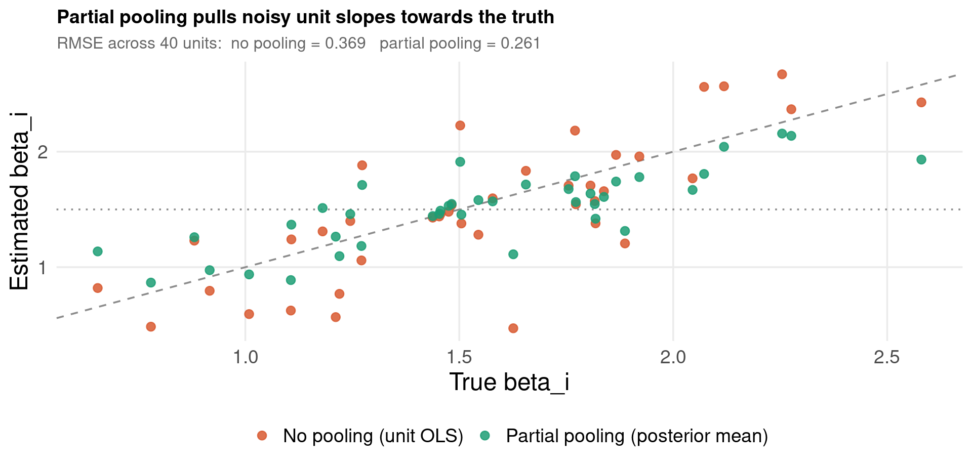
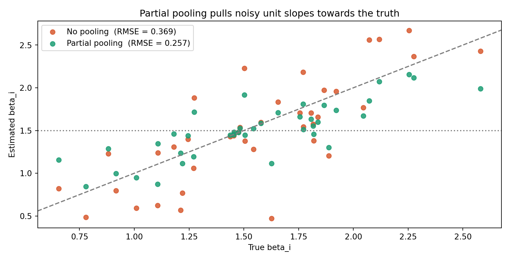
For every unit we now have two slope estimates and — uniquely, because this is simulated data — the true \(\beta_i\):

• No pooling: OLS on each unit’s 10 observations
• Partial pooling: the hierarchical posterior mean, shrunk towards \(\mu_\beta\)

If shrinkage works, the partial-pooling estimates should sit closer to the 45° line against the truth, and their RMSE across the 40 units should be smaller.

truth <- read.csv("../data/bayes-hp-sim-truth.csv")

# no-pooling slopes (one OLS per unit) vs hierarchical posterior means
slopes_np <- numeric(40)
for (i in 1:40) slopes_np[i] <- coef(lm(y ~ x, data = sim[sim$id == i, ]))[2]
slopes_pp <- coef(fit_rs)$id[, "Estimate", "x"]

df_shr <- data.frame(
  truth = rep(truth$beta_true, 2),
  est   = c(slopes_np, slopes_pp),
  method = rep(c("No pooling (unit OLS)", "Partial pooling (posterior mean)"),
               each = 40)
)
rmse_np <- sqrt(mean((slopes_np - truth$beta_true)^2))
rmse_pp <- sqrt(mean((slopes_pp - truth$beta_true)^2))

ggplot(df_shr, aes(x = truth, y = est, color = method)) +
  geom_abline(slope = 1, intercept = 0, linetype = "dashed", color = "grey55") +
  geom_hline(yintercept = 1.5, linetype = "dotted", color = "grey55") +
  geom_point(size = 2.6, alpha = 0.85) +
  scale_color_manual(values = c("#D85A30", "#1D9E75"), name = NULL) +
  labs(x = "True beta_i", y = "Estimated beta_i",
       title = "Partial pooling pulls noisy unit slopes towards the truth",
       subtitle = sprintf("RMSE across 40 units:  no pooling = %.3f   partial pooling = %.3f",
                          rmse_np, rmse_pp)) +
  theme_lecture

import numpy as np
import pandas as pd
import matplotlib.pyplot as plt

truth = pd.read_csv("../data/bayes-hp-sim-truth.csv")
b_pp = tr_rs.posterior["b"].mean(dim=["chain", "draw"]).values
b_np = np.array([np.polyfit(g["x"], g["y"], 1)[0] for _, g in sim.groupby("id")])
bt = truth["beta_true"].values

fig, ax = plt.subplots(figsize=(9, 4.6))
ax.axline((1, 1), slope=1, ls="--", color="grey")
ax.axhline(1.5, ls=":", color="grey")
ax.scatter(bt, b_np, color="#D85A30", s=35, alpha=0.85,
           label=f"No pooling  (RMSE = {np.sqrt(np.mean((b_np - bt)**2)):.3f})")
ax.scatter(bt, b_pp, color="#1D9E75", s=35, alpha=0.85,
           label=f"Partial pooling  (RMSE = {np.sqrt(np.mean((b_pp - bt)**2)):.3f})")
ax.set_xlabel("True beta_i"); ax.set_ylabel("Estimated beta_i")
ax.set_title("Partial pooling pulls noisy unit slopes towards the truth")
ax.legend()
plt.tight_layout(); plt.show()

Part IV: Priors, Convergence & Model Checking

Trust nothing until the chains, the priors and the predictions check out

Priors for Hierarchical Variance Components

• Theory

The variance components \(\tau_\alpha, \tau_\beta\) are the most prior-sensitive parameters in the model — they sit at the top of the hierarchy with only \(N\) “observations” (the unit effects) informing them.

• Bad: \(\text{InvGamma}(\epsilon, \epsilon)\) on \(\tau^2\) — spikes near zero, forces over-pooling when \(N\) is small, and is not non-informative despite its reputation
• Good: half-normal or half-\(t\) directly on the SD \(\tau\) — flat near zero, gentle decay (Gelman 2006)
• Correlations: \(\text{LKJ}(\eta)\) with \(\eta = 2\) mildly shrinks \(|\rho|\) away from 1 — with 10–40 units the correlation is weakly identified and needs this regularisation
• Rule of thumb: simulate from your priors (prior predictive) and check the implied data are merely plausible, not absurd

prior_summary(fit_rs)

                prior     class      coef group resp dpar nlpar lb ub tag
         normal(0, 5)         b                                          
         normal(0, 5)         b         x                                
         normal(0, 5) Intercept                                          
 lkj_corr_cholesky(2)         L                                          
 lkj_corr_cholesky(2)         L              id                          
         normal(0, 2)        sd                                  0       
         normal(0, 2)        sd              id                  0       
         normal(0, 2)        sd Intercept    id                  0       
         normal(0, 2)        sd         x    id                  0       
         normal(0, 2)     sigma                                  0       
       source
         user
 (vectorized)
         user
         user
 (vectorized)
         user
 (vectorized)
 (vectorized)
 (vectorized)
         user

* bayes: mixed default priors (used on the previous slides):
*   {y:x y:_cons}        ~ normal(0, 10000)      regression coefficients
*   {var(U0) var(U1)}    ~ igamma(0.01, 0.01)    random-effect variances
*   {var(e.y)}           ~ igamma(0.01, 0.01)    residual variance
* Custom priors are set with the prior() option, e.g.:
bayes, prior({y:x}, normal(0, 25))                 ///
       prior({var(U0)}, igamma(2, 1)):             ///
  mixed y x || id: x, covariance(independent)

Stata keeps inverse-gamma variance priors for conjugacy (Gibbs updates). With \(N = 40\) units this is harmless here — but re-run Part V’s 10-firm model with igamma(2, 1) and watch the firm-level variances move: small panels are prior-sensitive.

Convergence Diagnostics

• What to Check

Before believing any posterior summary:

• \(\widehat{R}\) (potential scale reduction): compares between-chain and within-chain variance; require \(\widehat{R} < 1.01\) for every parameter
• Effective sample size: MCMC draws are autocorrelated; ESS is the equivalent number of independent draws — worry below ~400 (bulk) for means, and check tail ESS for intervals
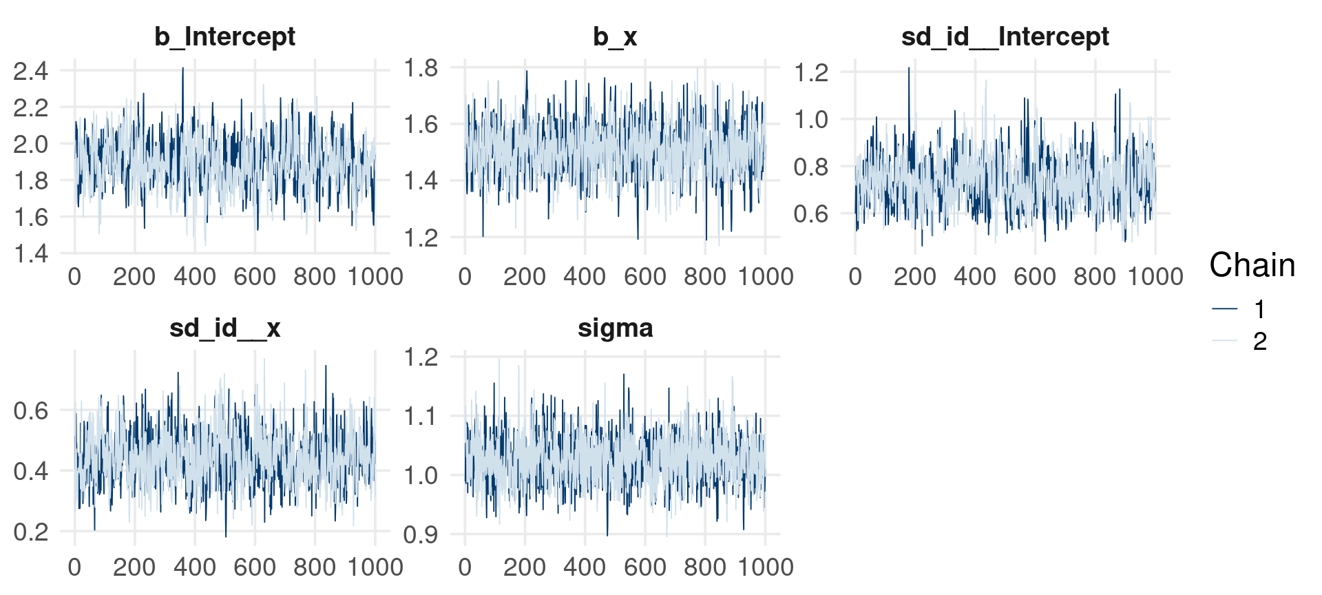
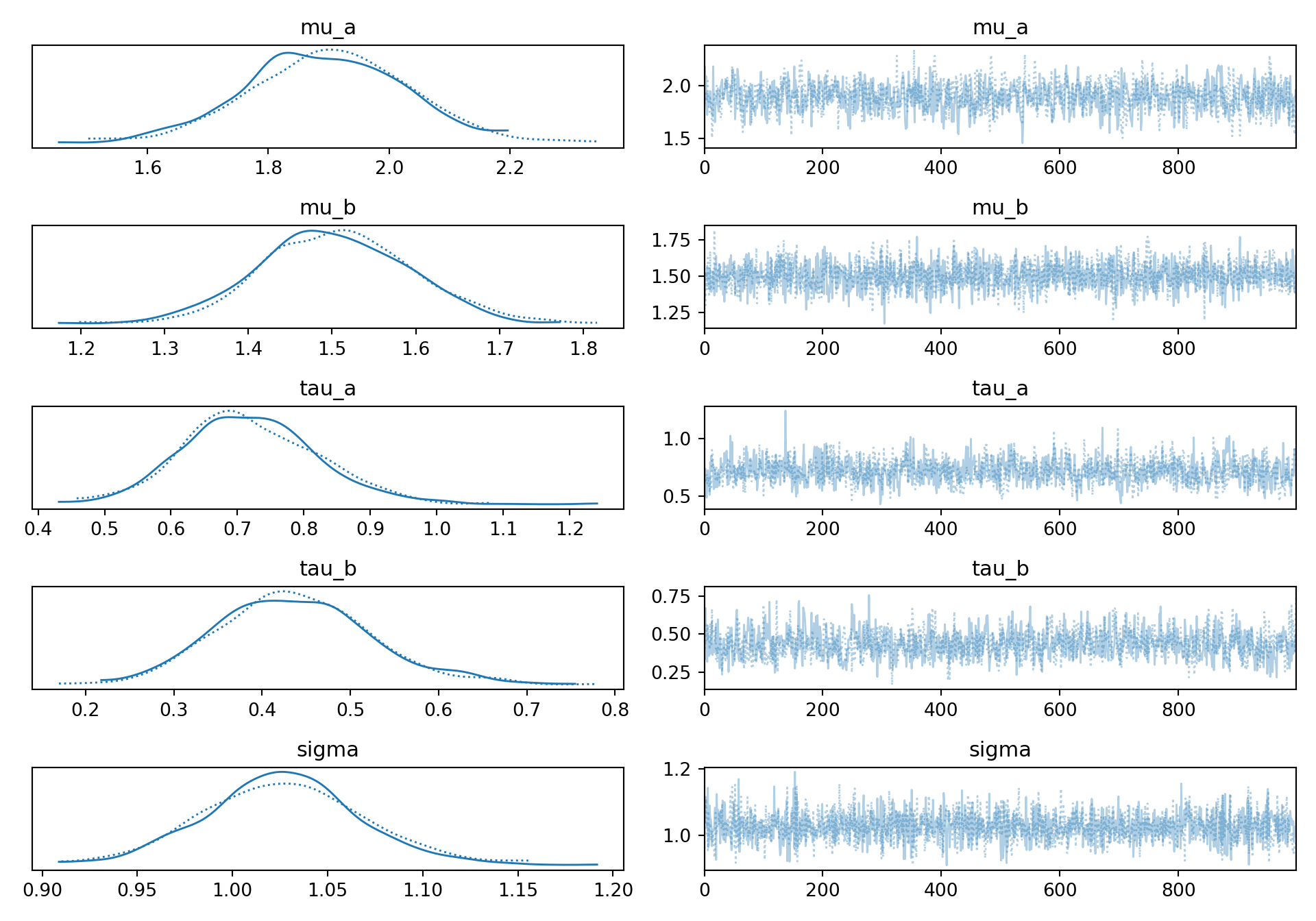
• Trace plots: chains should look like “fat hairy caterpillars” overlapping completely
• Divergent transitions (HMC only): even a handful signals the sampler could not follow the posterior geometry — reparameterise (non-centered) or tighten priors, never just ignore

\[ \widehat{R} = \sqrt{\frac{\widehat{\text{Var}}^{+}(\theta \mid y)}{W}}, \qquad \widehat{\text{Var}}^{+} = \frac{n-1}{n} W + \frac{1}{n} B \]

mcmc_trace(fit_rs, pars = c("b_Intercept", "b_x", "sd_id__Intercept",
                            "sd_id__x", "sigma"),
           facet_args = list(ncol = 3))

rhats <- brms::rhat(fit_rs)
cat(sprintf("max Rhat            : %.4f\n", max(rhats, na.rm = TRUE)))
cat(sprintf("min bulk ESS ratio  : %.3f\n", min(neff_ratio(fit_rs), na.rm = TRUE)))
cat(sprintf("divergent transitions: %d\n",
            sum(subset(nuts_params(fit_rs), Parameter == "divergent__")$Value)))

max Rhat            : 1.0070

min bulk ESS ratio  : 0.221

divergent transitions: 0

import arviz as az
import matplotlib.pyplot as plt

az.plot_trace(tr_rs, var_names=["mu_a", "mu_b", "tau_a", "tau_b", "sigma"],
              figsize=(10, 7))

array([[<Axes: title={'center': 'mu_a'}>,
        <Axes: title={'center': 'mu_a'}>],
       [<Axes: title={'center': 'mu_b'}>,
        <Axes: title={'center': 'mu_b'}>],
       [<Axes: title={'center': 'tau_a'}>,
        <Axes: title={'center': 'tau_a'}>],
       [<Axes: title={'center': 'tau_b'}>,
        <Axes: title={'center': 'tau_b'}>],
       [<Axes: title={'center': 'sigma'}>,
        <Axes: title={'center': 'sigma'}>]], dtype=object)

plt.tight_layout(); plt.show()

summ = az.summary(tr_rs, var_names=["mu_a", "mu_b", "tau_a", "tau_b", "sigma"])
print(summ[["ess_bulk", "ess_tail", "r_hat"]])

       ess_bulk  ess_tail  r_hat
mu_a      949.0     998.0    1.0
mu_b     1538.0    1360.0    1.0
tau_a     637.0     961.0    1.0
tau_b     866.0    1328.0    1.0
sigma    1720.0    1289.0    1.0

ndiv = int(tr_rs.sample_stats["diverging"].sum())
print(f"\ndivergent transitions: {ndiv}")

divergent transitions: 0

import delimited "../data/bayes-hp-sim.csv", clear
quietly destring _all, replace
quietly bayes, rseed(14159) mcmcsize(2500) burnin(2500): ///
  mixed y x || id: x, covariance(independent)
* effective sample sizes, then the 4-panel diagnostic plot for the slope
bayesstats ess {y:x} {y:_cons}
bayesgraph diagnostics {y:x}

(encoding automatically selected: ISO-8859-1)
(4 vars, 400 obs)




Efficiency summaries    MCMC sample size =     2,500
                        Efficiency:  min =    .03683
                                     avg =    .03721
                                     max =     .0376

----------------------------------------------------
          y  |        ESS   Corr. time    Efficiency
-------------+--------------------------------------
           x |      93.99        26.60        0.0376
       _cons |      92.07        27.15        0.0368
----------------------------------------------------

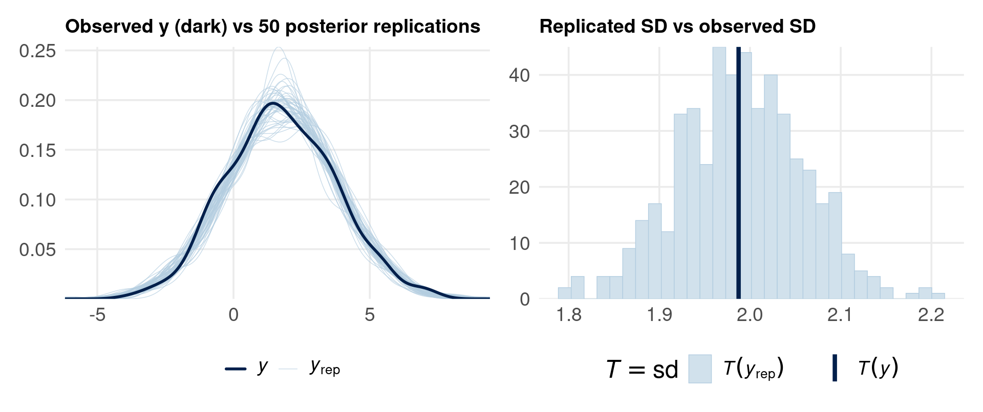
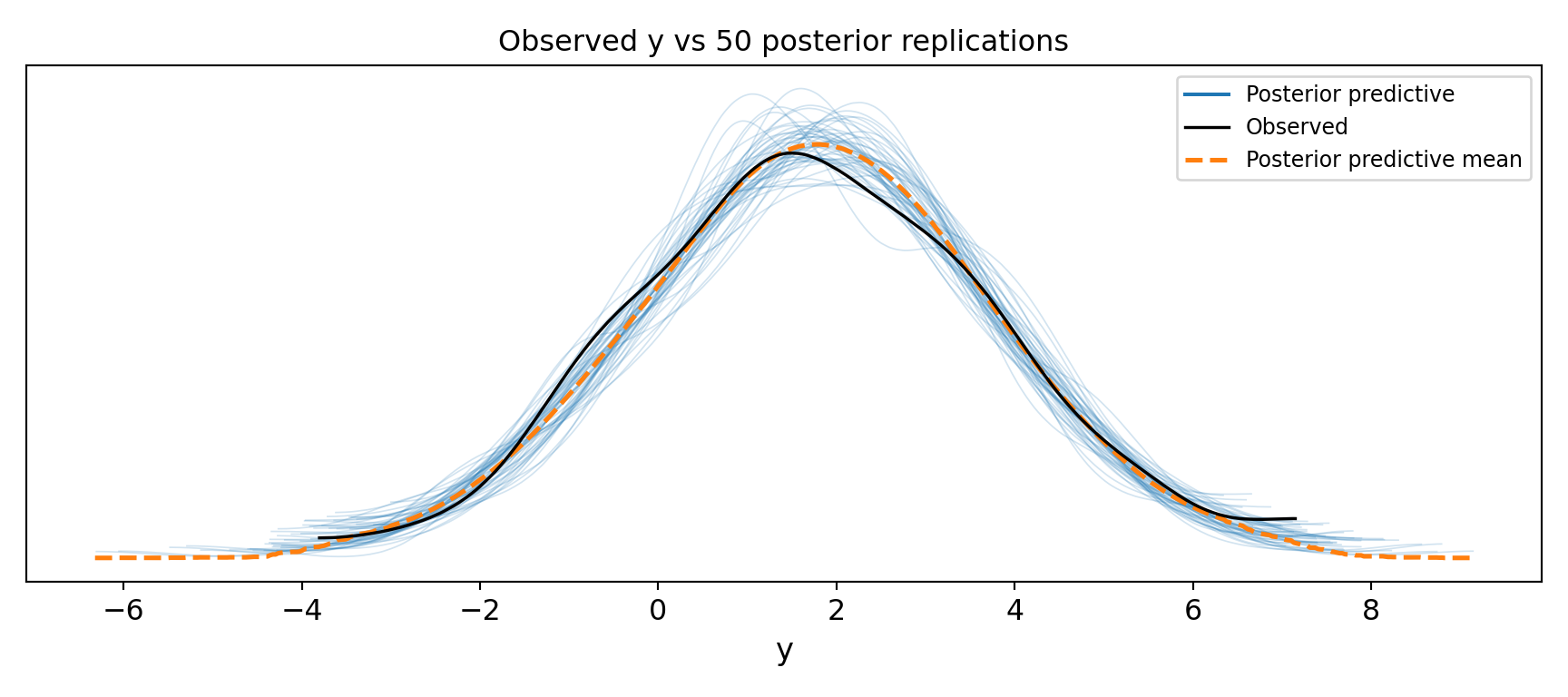
Posterior Predictive Checks

• The Idea

If the model is adequate, data simulated from the posterior should look like the data we observed:

\[ y^{\text{rep}} \sim p(y^{\text{rep}} \mid y) = \int p(y^{\text{rep}} \mid \theta)\, p(\theta \mid y)\, d\theta \]

• Overlay the density of \(y\) on densities of many \(y^{\text{rep}}\) draws — systematic gaps mean model misfit
• Compare test statistics: if the observed statistic sits in the tails of its replicated distribution, that feature of the data is not captured
• PPCs test adequacy, not truth — a model can pass and still omit the economics you care about

p1 <- pp_check(fit_rs, ndraws = 50) +
  labs(title = "Observed y (dark) vs 50 posterior replications") +
  theme_lecture
p2 <- pp_check(fit_rs, type = "stat", stat = "sd", ndraws = 500) +
  labs(title = "Replicated SD vs observed SD") +
  theme_lecture
p1 + p2

import pymc as pm
import arviz as az
import matplotlib.pyplot as plt

with m_rs:
    ppc = pm.sample_posterior_predictive(tr_rs, random_seed=14159,
                                         progressbar=False)

az.plot_ppc(ppc, num_pp_samples=50, figsize=(9, 4))
plt.title("Observed y vs 50 posterior replications")
plt.tight_layout(); plt.show()

Model Comparison — LOO and WAIC

• Theory

Which pooling level does the data prefer? Compare models by out-of-sample predictive accuracy, estimated without refitting via Pareto-smoothed importance sampling (Vehtari, Gelman & Gabry 2017):

\[ \widehat{\text{elpd}}_{\text{loo}} = \sum_{n=1}^{N T} \log \hat{p}(y_n \mid y_{-n}) \]

• Higher elpd = better predictions; differences smaller than ~2 SE are not decisive
• WAIC is an asymptotically equivalent information criterion; LOO is more robust and diagnoses its own failures (Pareto \(\hat{k}\))
• We compare three nested models on the simulated panel: complete pooling, random intercepts, random intercepts + slopes (the truth)

fit_pool <- brm(y ~ x, data = sim,
                chains = 2, iter = 2000, warmup = 1000, cores = 2,
                seed = 14159, refresh = 0, silent = 2)
fit_ri   <- brm(y ~ x + (1 | id), data = sim,
                chains = 2, iter = 2000, warmup = 1000, cores = 2,
                seed = 14159, refresh = 0, silent = 2)

loo_pool <- loo(fit_pool)
loo_ri   <- loo(fit_ri)
loo_rs   <- loo(fit_rs)
loo_compare(loo_pool, loo_ri, loo_rs)

Model comparison (best model on top, elpd differences):

         elpd_diff se_diff
fit_rs     0.0       0.0  
fit_ri   -18.1       5.8  
fit_pool -64.7      10.0  

fit_rs = intercepts + slopes (the true DGP), fit_ri = intercepts only, fit_pool = complete pooling

import pymc as pm
import arviz as az

# two simpler competitors, same data
with pm.Model() as m_pool:
    a0 = pm.Normal("a0", 0, 5)
    b0 = pm.Normal("b0", 0, 5)
    s0 = pm.HalfNormal("s0", 2)
    pm.Normal("y", a0 + b0 * sim["x"].values, s0, observed=sim["y"].values)
    tr_pool = pm.sample(1000, tune=1000, chains=2, cores=2, random_seed=14159,
                        progressbar=False, idata_kwargs={"log_likelihood": True})

y

with pm.Model() as m_ri:
    mu_a = pm.Normal("mu_a", 0, 5)
    tau_a = pm.HalfNormal("tau_a", 2)
    za = pm.Normal("za", 0, 1, shape=len(ids))
    b0 = pm.Normal("b0", 0, 5)
    s0 = pm.HalfNormal("s0", 2)
    pm.Normal("y", mu_a + tau_a * za[idx] + b0 * sim["x"].values, s0,
              observed=sim["y"].values)
    tr_ri = pm.sample(1000, tune=1000, chains=2, cores=2, random_seed=14159,
                      progressbar=False, idata_kwargs={"log_likelihood": True})

y

comp = az.compare({"pooled": tr_pool, "rand intercept": tr_ri,
                   "rand int + slope": tr_rs}, ic="loo")
print(comp[["rank", "elpd_loo", "elpd_diff", "dse"]].round(2))

                  rank  elpd_loo  elpd_diff    dse
rand int + slope     0   -610.48       0.00   0.00
rand intercept       1   -628.45      17.97   5.84
pooled               2   -674.58      64.10  10.04

Part V: Real Data I — The Grunfeld Investment Panel

Random-coefficient investment equations for 10 US firms, 1935–1954

The Grunfeld Data

• The Story

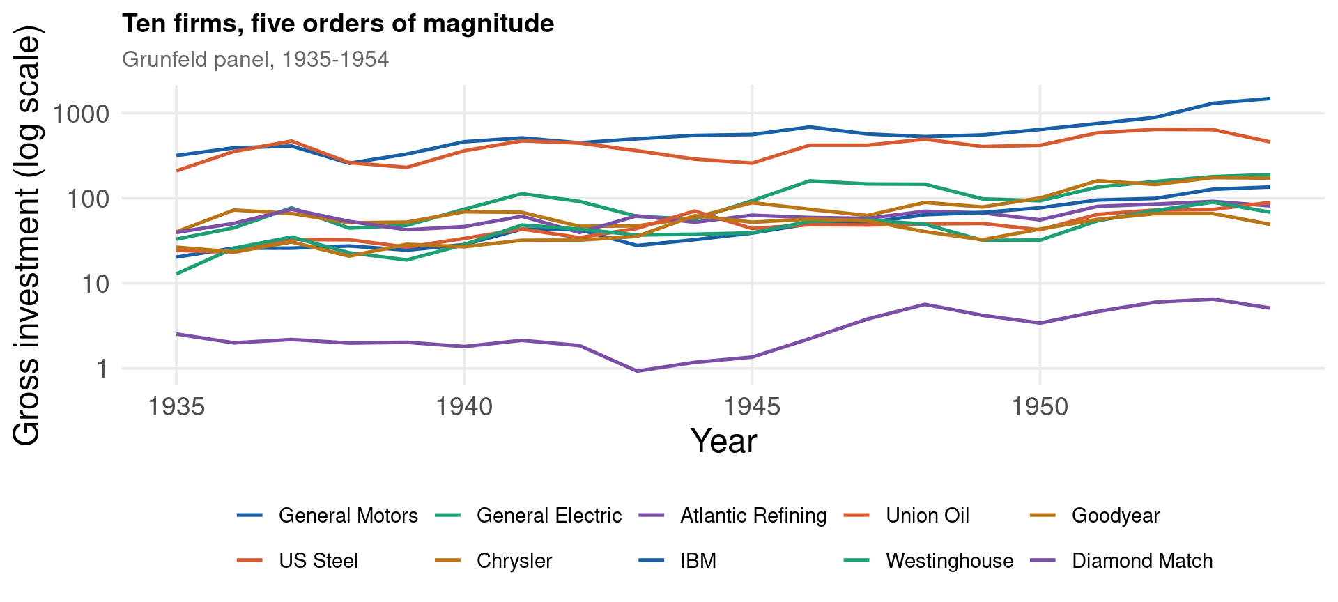
The most re-used panel in econometrics (Kleiber & Zeileis 2010): 10 large US firms observed annually 1935–1954.

\[ \text{inv}_{it} = \text{gross investment}, \qquad \text{value}_{it} = \text{market value of the firm}, \qquad \text{capital}_{it} = \text{capital stock} \]

• The units range from General Motors to Diamond Match — five orders of magnitude apart in size, so firm heterogeneity is not a nuisance, it is the point
• Only \(N = 10\) firms: exactly the small-\(N\) regime where variance components are hard to pin down and priors matter
• We model the standardised variables (inv_s, value_s, capital_s, computed once in bayesian-hp-data.R) so all three engines share identical scales and priors

grun <- read.csv("../data/bayes-hp-grunfeld.csv")
firm_names <- c("General Motors", "US Steel", "General Electric", "Chrysler",
                "Atlantic Refining", "IBM", "Union Oil", "Westinghouse",
                "Goodyear", "Diamond Match")
grun$firm_lab <- factor(firm_names[grun$firm], levels = firm_names)

ggplot(grun, aes(x = year, y = inv, color = firm_lab)) +
  geom_line(linewidth = 0.9) +
  scale_y_log10() +
  scale_color_manual(values = rep(c("#185FA5", "#D85A30", "#1D9E75",
                                    "#BA7517", "#7B4FA6"), 2)) +
  labs(x = "Year", y = "Gross investment (log scale)", color = NULL,
       title = "Ten firms, five orders of magnitude",
       subtitle = "Grunfeld panel, 1935-1954") +
  theme_lecture + theme(legend.text = element_text(size = 11))

import pandas as pd

grun = pd.read_csv("../data/bayes-hp-grunfeld.csv")
tab = grun.groupby("firm")[["inv", "value", "capital"]].mean().round(1)
tab.index = ["General Motors", "US Steel", "General Electric", "Chrysler",
             "Atlantic Refining", "IBM", "Union Oil", "Westinghouse",
             "Goodyear", "Diamond Match"]
print("Firm means, 1935-1954 (millions of 1947 USD):\n")

Firm means, 1935-1954 (millions of 1947 USD):

print(tab.to_string())

                     inv   value  capital
General Motors     608.0  4333.8    648.4
US Steel           410.5  1971.8    294.9
General Electric   102.3  1941.3    400.2
Chrysler            86.1   693.2    121.2
Atlantic Refining   61.8   231.5    486.8
IBM                 55.4   419.9    104.3
Union Oil           47.6   149.8    314.9
Westinghouse        42.9   670.9     85.6
Goodyear            41.9   333.6    297.9
Diamond Match        3.1    70.9      5.9

import delimited "../data/bayes-hp-grunfeld.csv", clear
quietly destring _all, replace
xtset firm year
xtsum inv value capital

(encoding automatically selected: ISO-8859-1)
(8 vars, 200 obs)



Panel variable: firm (strongly balanced)
 Time variable: year, 1935 to 1954
         Delta: 1 unit


Variable         |      Mean   Std. dev.       Min        Max |    Observations
-----------------+--------------------------------------------+----------------
inv      overall |  145.9583   216.8753        .93     1486.7 |     N =     200
         between |             198.8242     3.0845     608.02 |     n =      10
         within  |             106.1986  -204.3617   1024.638 |     T =      20
                 |                                            |
value    overall |  1081.681    1314.47      58.12     6241.7 |     N =     200
         between |             1334.917     70.921   4333.845 |     n =      10
         within  |             340.5421   -459.964   2989.536 |     T =      20
                 |                                            |
capital  overall |  276.0172   301.1039         .8     2226.3 |     N =     200
         between |             200.9701     5.9415    648.435 |     n =      10
         within  |             232.6603  -369.6179   1853.882 |     T =      20

A Random-Coefficients Investment Equation

• The Model

The Grunfeld equation with firm-specific coefficients — Swamy’s (1970) random-coefficients model, done properly by MCMC:

\[ \text{inv}^s_{it} = \alpha_i + \beta_{1i}\, \text{value}^s_{it} + \beta_{2i}\, \text{capital}^s_{it} + \varepsilon_{it} \]

\[ (\alpha_i, \beta_{1i}, \beta_{2i}) \sim \mathcal{N}(\boldsymbol{\mu}, \boldsymbol{\Sigma}), \qquad \varepsilon_{it} \sim \mathcal{N}(0, \sigma^2) \]

• Does every firm turn market value into investment at the same rate? The posterior for \(\tau_{\beta_1}\) answers directly
• With \(N = 10\) firms, no-pooling OLS gives 10 noisy answers and pooled OLS one wrong one — partial pooling is the honest middle

priors_g <- c(prior(normal(0, 2), class = Intercept),
              prior(normal(0, 2), class = b),
              prior(normal(0, 1), class = sd),
              prior(normal(0, 1), class = sigma),
              prior(lkj(2),       class = cor))

fit_grun <- brm(inv_s ~ value_s + capital_s + (1 + value_s + capital_s | firm),
                data = grun, prior = priors_g,
                chains = 2, iter = 2000, warmup = 1000, cores = 2,
                seed = 14159, refresh = 0, silent = 2,
                control = list(adapt_delta = 0.95))
summary(fit_grun)

 Family: gaussian 
  Links: mu = identity 
Formula: inv_s ~ value_s + capital_s + (1 + value_s + capital_s | firm) 
   Data: grun (Number of observations: 200) 
  Draws: 2 chains, each with iter = 2000; warmup = 1000; thin = 1;
         total post-warmup draws = 2000

Multilevel Hyperparameters:
~firm (Number of levels: 10) 
                         Estimate Est.Error l-95% CI u-95% CI Rhat Bulk_ESS
sd(Intercept)                0.29      0.09     0.16     0.51 1.00      807
sd(value_s)                  0.34      0.12     0.15     0.64 1.00      799
sd(capital_s)                0.21      0.08     0.11     0.40 1.01      867
cor(Intercept,value_s)       0.67      0.23     0.07     0.96 1.00      998
cor(Intercept,capital_s)     0.34      0.29    -0.29     0.82 1.00      989
cor(value_s,capital_s)       0.23      0.34    -0.45     0.80 1.00      736
                         Tail_ESS
sd(Intercept)                1125
sd(value_s)                  1179
sd(capital_s)                 977
cor(Intercept,value_s)       1232
cor(Intercept,capital_s)     1066
cor(value_s,capital_s)       1169

Regression Coefficients:
          Estimate Est.Error l-95% CI u-95% CI Rhat Bulk_ESS Tail_ESS
Intercept    -0.08      0.12    -0.30     0.16 1.00      589      918
value_s       0.53      0.17     0.20     0.87 1.00      673      767
capital_s     0.27      0.09     0.09     0.43 1.00      864      926

Further Distributional Parameters:
      Estimate Est.Error l-95% CI u-95% CI Rhat Bulk_ESS Tail_ESS
sigma     0.20      0.01     0.18     0.22 1.00     2763     1388

Draws were sampled using sampling(NUTS). For each parameter, Bulk_ESS
and Tail_ESS are effective sample size measures, and Rhat is the potential
scale reduction factor on split chains (at convergence, Rhat = 1).

import warnings
warnings.filterwarnings("ignore")
import pandas as pd
import pymc as pm
import arviz as az

grun = pd.read_csv("../data/bayes-hp-grunfeld.csv")
fidx, firms = pd.factorize(grun["firm"])

with pm.Model() as m_grun:
    mu = pm.Normal("mu", 0, 2, shape=3)          # (intercept, value, capital)
    tau = pm.HalfNormal("tau", 1, shape=3)
    z = pm.Normal("z", 0, 1, shape=(3, len(firms)))
    coefs = pm.Deterministic("coefs", mu[:, None] + tau[:, None] * z)
    sigma = pm.HalfNormal("sigma", 1)
    mean = (coefs[0, fidx] + coefs[1, fidx] * grun["value_s"].values
            + coefs[2, fidx] * grun["capital_s"].values)
    pm.Normal("inv_s", mean, sigma, observed=grun["inv_s"].values)
    tr_grun = pm.sample(1000, tune=1500, chains=2, cores=2,
                        random_seed=14159, progressbar=False,
                        target_accept=0.95)

inv_s

print(az.summary(tr_grun, var_names=["mu", "tau", "sigma"]).round(3))

         mean     sd  hdi_3%  hdi_97%  ...  mcse_sd  ess_bulk  ess_tail  r_hat
mu[0]  -0.058  0.120  -0.272    0.179  ...    0.003    1064.0    1092.0    1.0
mu[1]   0.565  0.165   0.267    0.880  ...    0.005    1320.0    1199.0    1.0
mu[2]   0.278  0.091   0.098    0.430  ...    0.003     958.0    1186.0    1.0
tau[0]  0.313  0.105   0.144    0.517  ...    0.004    1106.0    1258.0    1.0
tau[1]  0.364  0.139   0.144    0.623  ...    0.004    1467.0    1283.0    1.0
tau[2]  0.219  0.078   0.096    0.361  ...    0.003    1122.0    1147.0    1.0
sigma   0.199  0.011   0.177    0.220  ...    0.000    3243.0    1030.0    1.0

[7 rows x 9 columns]

import delimited "../data/bayes-hp-grunfeld.csv", clear
quietly destring _all, replace
bayes, rseed(14159) mcmcsize(2500) burnin(2500): ///
  mixed inv_s value_s capital_s || firm: value_s capital_s, covariance(independent)

(encoding automatically selected: ISO-8859-1)
(8 vars, 200 obs)


note: Gibbs sampling is used for regression coefficients and variance
      components.

Burn-in 2500 aaaaaaaaa1000aaaaaaaaa2000aaaaa done
Simulation 2500 .........1000.........2000..... done

Multilevel structure
------------------------------------------------------------------------------
firm
    {U0}: random intercepts
    {U1}: random coefficients for value_s
    {U2}: random coefficients for capital_s
------------------------------------------------------------------------------

Model summary
------------------------------------------------------------------------------
Likelihood: 
  inv_s ~ normal(xb_inv_s,{e.inv_s:sigma2})

Priors: 
  {inv_s:value_s capital_s _cons} ~ normal(0,10000)                        (1)
                             {U0} ~ normal(0,{U0:sigma2})                  (1)
                             {U1} ~ normal(0,{U1:sigma2})                  (1)
                             {U2} ~ normal(0,{U2:sigma2})                  (1)
                 {e.inv_s:sigma2} ~ igamma(.01,.01)

Hyperpriors: 
  {U0:sigma2} ~ igamma(.01,.01)
  {U1:sigma2} ~ igamma(.01,.01)
  {U2:sigma2} ~ igamma(.01,.01)
------------------------------------------------------------------------------
(1) Parameters are elements of the linear form xb_inv_s.

Bayesian multilevel regression                   MCMC iterations  =      5,000
Metropolis–Hastings and Gibbs sampling           Burn-in          =      2,500
                                                 MCMC sample size =      2,500
Group variable: firm                             Number of groups =         10
                                                 Obs per group:
                                                              min =         20
                                                              avg =       20.0
                                                              max =         20
                                                 Number of obs    =        200
                                                 Acceptance rate  =      .7424
                                                 Efficiency:  min =    .003359
                                                              avg =      .0939
Log marginal-likelihood                                       max =      .5143

------------------------------------------------------------------------------
             |                                                Equal-tailed
             |      Mean   Std. dev.     MCSE     Median  [95% cred. interval]
-------------+----------------------------------------------------------------
inv_s        |
     value_s |  .5474894   .1272203   .043903   .5610818   .2952109   .7524473
   capital_s |  .3313063   .1665682    .05176   .3443998  -.0840036   .5842809
       _cons | -.0649826    .134059   .036025  -.0582597  -.3278946   .1706248
-------------+----------------------------------------------------------------
firm         |
   U0:sigma2 |  .1178473     .07983   .006285   .0980914   .0350814   .3267856
   U1:sigma2 |  .1379313   .1075998   .010385   .1099134   .0272493   .3978944
   U2:sigma2 |  .0773361   .0660366   .008817    .056464   .0158845   .2500928
-------------+----------------------------------------------------------------
e.inv_s      |
      sigma2 |  .0405176   .0084391   .000235   .0394661   .0322807   .0530224
------------------------------------------------------------------------------
Note: Default priors are used for model parameters.
Note: There is a high autocorrelation after 500 lags.

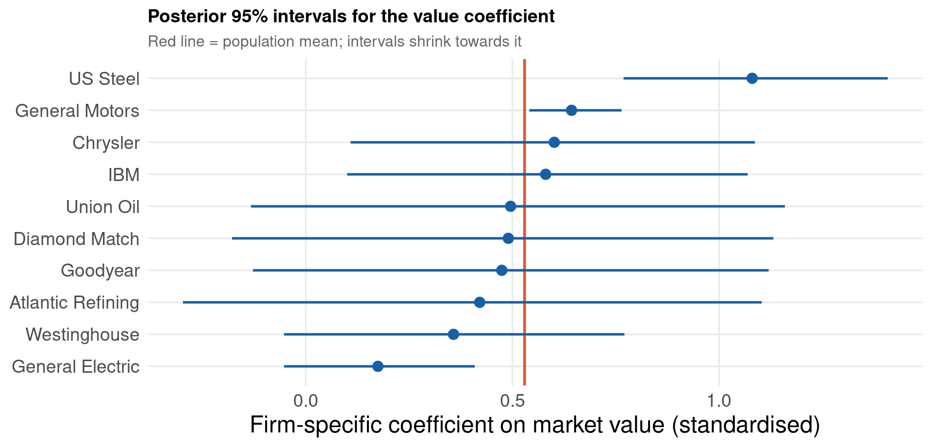
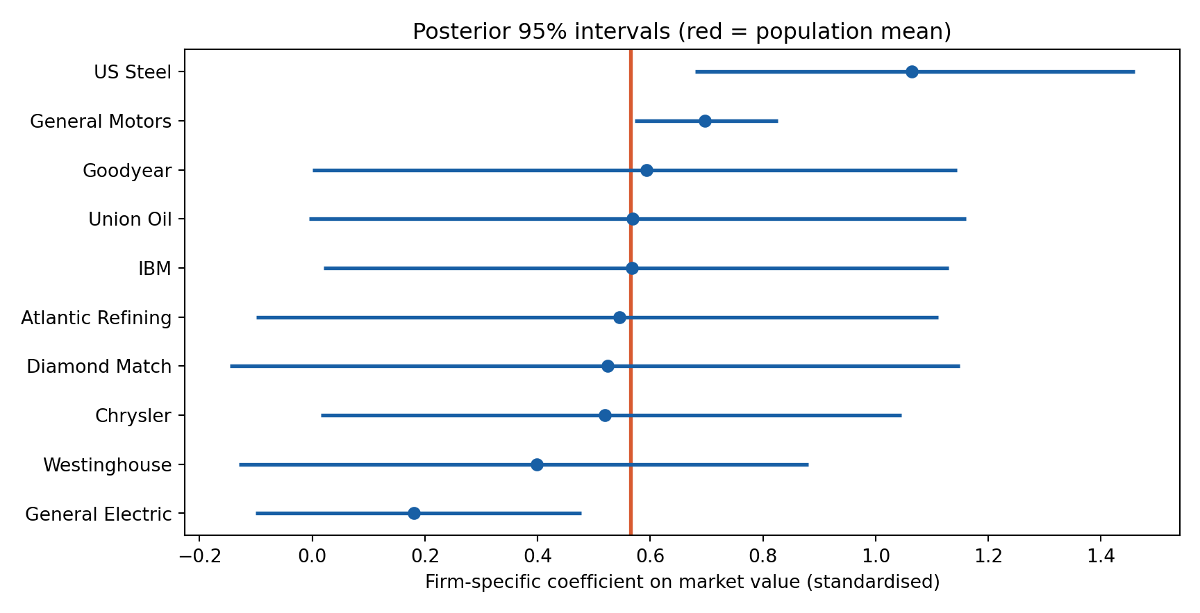
Firm-Level Posteriors — Who Invests Differently?

ce <- coef(fit_grun)$firm[, , "value_s"]
df_cat <- data.frame(firm = firm_names, est = ce[, "Estimate"],
                     lo = ce[, "Q2.5"], hi = ce[, "Q97.5"])
df_cat <- df_cat[order(df_cat$est), ]
df_cat$firm <- factor(df_cat$firm, levels = df_cat$firm)

ggplot(df_cat, aes(x = est, y = firm)) +
  geom_vline(xintercept = fixef(fit_grun)["value_s", "Estimate"],
             color = "#D85A30", linewidth = 1) +
  geom_pointrange(aes(xmin = lo, xmax = hi), color = "#185FA5",
                  linewidth = 0.9, size = 0.6) +
  labs(x = "Firm-specific coefficient on market value (standardised)",
       y = NULL, title = "Posterior 95% intervals for the value coefficient",
       subtitle = "Red line = population mean; intervals shrink towards it") +
  theme_lecture

import arviz as az
import matplotlib.pyplot as plt

names = ["General Motors", "US Steel", "General Electric", "Chrysler",
         "Atlantic Refining", "IBM", "Union Oil", "Westinghouse",
         "Goodyear", "Diamond Match"]
bval = tr_grun.posterior["coefs"].sel(coefs_dim_0=1)   # value_s coefficients

fig, ax = plt.subplots(figsize=(9, 4.6))
means = bval.mean(dim=["chain", "draw"]).values
lo = bval.quantile(0.025, dim=["chain", "draw"]).values
hi = bval.quantile(0.975, dim=["chain", "draw"]).values
order = means.argsort()
ax.axvline(tr_grun.posterior["mu"].sel(mu_dim_0=1).mean(), color="#D85A30", lw=2)
ax.hlines(range(len(names)), lo[order], hi[order], color="#185FA5", lw=2)
ax.plot(means[order], range(len(names)), "o", color="#185FA5", ms=6)
ax.set_yticks(range(len(names)))
ax.set_yticklabels([names[i] for i in order])
ax.set_xlabel("Firm-specific coefficient on market value (standardised)")
ax.set_title("Posterior 95% intervals (red = population mean)")
plt.tight_layout(); plt.show()

Part VI: Real Data II — Union Wages

The union premium in the Vella–Verbeek young-men panel

The wagepan Data & the Question

• The Story

Vella & Verbeek (1998): US young men from the NLSY, followed 1980–1987 — the wagepan data in the wooldridge package.

• Question: how much more do union members earn, holding observables fixed?
• Outcome lwage (log hourly wage); key regressor union; controls married, exper, expersq, plus the time-invariant educ, black, hisp
• We use a random subsample of 150 men × 8 years = 1,200 observations (drawn in bayesian-hp-data.R) so the MCMC slides run in classroom time
• Persistent worker heterogeneity (ability, motivation) makes this a textbook case for person-specific intercepts

wp <- read.csv("../data/bayes-hp-wagepan.csv")
cat("men:", length(unique(wp$nr)), "  years:", length(unique(wp$year)),
    "  rows:", nrow(wp), "\n\n")
wp |>
  group_by(union) |>
  summarise(mean_lwage = mean(lwage), sd_lwage = sd(lwage), share = n() / nrow(wp))

men: 150   years: 8   rows: 1200 

  union mean_lwage sd_lwage share
1     0       1.66    0.478 0.767
2     1       1.85    0.466 0.233

Raw union gap: 0.191 log points

import pandas as pd

wp = pd.read_csv("../data/bayes-hp-wagepan.csv")
print(wp.groupby("union")["lwage"].agg(["mean", "std", "count"]).round(3))

        mean    std  count
union                     
0      1.655  0.478    921
1      1.846  0.466    279

gap = wp.loc[wp.union == 1, "lwage"].mean() - wp.loc[wp.union == 0, "lwage"].mean()
print(f"\nRaw union gap: {gap:.3f} log points")

Raw union gap: 0.191 log points

import delimited "../data/bayes-hp-wagepan.csv", clear
quietly destring _all, replace
xtset nr year
tabstat lwage, by(union) statistics(mean sd n) format(%9.3f)

(encoding automatically selected: ISO-8859-1)
(10 vars, 1,200 obs)



Panel variable: nr (strongly balanced)
 Time variable: year, 1980 to 1987
         Delta: 1 unit


Summary for variables: lwage
Group variable: union 

   union |      Mean        SD         N
---------+------------------------------
       0 |     1.655     0.478   921.000
       1 |     1.846     0.466   279.000
---------+------------------------------
   Total |     1.700     0.482  1200.000
----------------------------------------

Hierarchical Wage Regression

• The Model

Person-specific intercepts absorb persistent unobserved skill; the union premium \(\beta_1\) is common:

\[ \text{lwage}_{it} = \alpha_i + \beta_1 \text{union}_{it} + \beta_2 \text{married}_{it} + \beta_3 \text{exper}_{it} + \beta_4 \text{exper}^2_{it} + \mathbf{x}_i'\boldsymbol{\gamma} + \varepsilon_{it} \]

\[ \alpha_i \sim \mathcal{N}(\mu_\alpha, \tau_\alpha^2), \qquad \beta_j, \gamma_j \sim \mathcal{N}(0, 0.5^2), \qquad \tau_\alpha, \sigma \sim \mathcal{N}^{+}(0, 1) \]

• \(\mathbf{x}_i = (\text{educ}, \text{black}, \text{hisp})\) are time-invariant — estimable here, impossible under fixed effects
• The \(\mathcal{N}(0, 0.5^2)\) coefficient prior says: effects above 50 log points are implausible — weakly informative on the economics
• In R we also draw from the prior (sample_prior = "yes") — needed for the Savage–Dickey test in Part VII

priors_w <- c(prior(normal(0, 5),   class = Intercept),
              prior(normal(0, 0.5), class = b),
              prior(normal(0, 1),   class = sd),
              prior(normal(0, 1),   class = sigma))

fit_wage <- brm(lwage ~ union + married + exper + expersq + educ + black + hisp
                + (1 | nr),
                data = wp, prior = priors_w, sample_prior = "yes",
                chains = 2, iter = 2000, warmup = 1000, cores = 2,
                seed = 14159, refresh = 0, silent = 2)
summary(fit_wage)

 Family: gaussian 
  Links: mu = identity 
Formula: lwage ~ union + married + exper + expersq + educ + black + hisp + (1 | nr) 
   Data: wp (Number of observations: 1200) 
  Draws: 2 chains, each with iter = 2000; warmup = 1000; thin = 1;
         total post-warmup draws = 2000

Multilevel Hyperparameters:
~nr (Number of levels: 150) 
              Estimate Est.Error l-95% CI u-95% CI Rhat Bulk_ESS Tail_ESS
sd(Intercept)     0.28      0.02     0.25     0.32 1.00      768     1038

Regression Coefficients:
          Estimate Est.Error l-95% CI u-95% CI Rhat Bulk_ESS Tail_ESS
Intercept     0.02      0.19    -0.36     0.41 1.00      669     1029
union         0.12      0.03     0.06     0.18 1.00     1922     1888
married       0.05      0.03    -0.01     0.11 1.00     1569     1624
exper         0.12      0.02     0.09     0.15 1.00     2987     1695
expersq      -0.00      0.00    -0.01    -0.00 1.00     3361     1763
educ          0.09      0.02     0.06     0.12 1.00      631     1034
black        -0.17      0.09    -0.34     0.01 1.00      604     1199
hisp         -0.01      0.07    -0.15     0.13 1.01      486      945

Further Distributional Parameters:
      Estimate Est.Error l-95% CI u-95% CI Rhat Bulk_ESS Tail_ESS
sigma     0.33      0.01     0.32     0.34 1.00     2985     1503

Draws were sampled using sampling(NUTS). For each parameter, Bulk_ESS
and Tail_ESS are effective sample size measures, and Rhat is the potential
scale reduction factor on split chains (at convergence, Rhat = 1).

import warnings
warnings.filterwarnings("ignore")
import pandas as pd
import numpy as np
import pymc as pm
import arviz as az

wp = pd.read_csv("../data/bayes-hp-wagepan.csv")
pidx, persons = pd.factorize(wp["nr"])
X = wp[["union", "married", "exper", "expersq", "educ", "black", "hisp"]].values
xnames = ["union", "married", "exper", "expersq", "educ", "black", "hisp"]

with pm.Model(coords={"coef": xnames}) as m_wage:
    mu_a = pm.Normal("mu_a", 0, 5)
    tau_a = pm.HalfNormal("tau_a", 1)
    za = pm.Normal("za", 0, 1, shape=len(persons))
    beta = pm.Normal("beta", 0, 0.5, dims="coef")
    sigma = pm.HalfNormal("sigma", 1)
    mean = mu_a + tau_a * za[pidx] + pm.math.dot(X, beta)
    pm.Normal("lwage", mean, sigma, observed=wp["lwage"].values)
    tr_wage = pm.sample(1000, tune=1000, chains=2, cores=2,
                        random_seed=14159, progressbar=False)

lwage

print(az.summary(tr_wage, var_names=["mu_a", "beta", "tau_a", "sigma"],
                 hdi_prob=0.95).round(3))

                mean     sd  hdi_2.5%  ...  ess_bulk  ess_tail  r_hat
mu_a           0.035  0.198    -0.346  ...     304.0     660.0   1.01
beta[union]    0.119  0.031     0.060  ...    1263.0    1438.0   1.00
beta[married]  0.055  0.029     0.002  ...    1072.0     955.0   1.00
beta[exper]    0.117  0.016     0.090  ...    1094.0    1378.0   1.00
beta[expersq] -0.004  0.001    -0.007  ...    1074.0    1420.0   1.00
beta[educ]     0.092  0.016     0.062  ...     316.0     665.0   1.01
beta[black]   -0.173  0.095    -0.363  ...     473.0     615.0   1.00
beta[hisp]    -0.007  0.069    -0.141  ...     315.0     613.0   1.01
tau_a          0.281  0.019     0.244  ...     514.0     934.0   1.01
sigma          0.330  0.007     0.317  ...    1785.0    1331.0   1.00

[10 rows x 9 columns]

import delimited "../data/bayes-hp-wagepan.csv", clear
quietly destring _all, replace
bayes, rseed(14159) mcmcsize(2500) burnin(2500) ///
  prior({lwage:union married exper expersq educ black hisp}, normal(0, 0.25)): ///
  mixed lwage union married exper expersq educ black hisp || nr:

(encoding automatically selected: ISO-8859-1)
(10 vars, 1,200 obs)


note: Gibbs sampling is used for regression coefficients and variance
      components.

Burn-in 2500 aaaaaaaaa1000aaaaaaaaa2000aaaaa done
Simulation 2500 .........1000.........2000..... done

Multilevel structure
------------------------------------------------------------------------------
nr
    {U0}: random intercepts
------------------------------------------------------------------------------

Model summary
------------------------------------------------------------------------------
Likelihood: 
  lwage ~ normal(xb_lwage,{e.lwage:sigma2})

Priors: 
     {lwage:union} ~ normal(0,0.25)                                        (1)
   {lwage:married} ~ normal(0,0.25)                                        (1)
     {lwage:exper} ~ normal(0,0.25)                                        (1)
   {lwage:expersq} ~ normal(0,0.25)                                        (1)
      {lwage:educ} ~ normal(0,0.25)                                        (1)
     {lwage:black} ~ normal(0,0.25)                                        (1)
      {lwage:hisp} ~ normal(0,0.25)                                        (1)
     {lwage:_cons} ~ normal(0,10000)                                       (1)
              {U0} ~ normal(0,{U0:sigma2})                                 (1)
  {e.lwage:sigma2} ~ igamma(.01,.01)

Hyperprior: 
  {U0:sigma2} ~ igamma(.01,.01)
------------------------------------------------------------------------------
(1) Parameters are elements of the linear form xb_lwage.

Bayesian multilevel regression                   MCMC iterations  =      5,000
Metropolis–Hastings and Gibbs sampling           Burn-in          =      2,500
                                                 MCMC sample size =      2,500
Group variable: nr                               Number of groups =        150
                                                 Obs per group:
                                                              min =          8
                                                              avg =        8.0
                                                              max =          8
                                                 Number of obs    =      1,200
                                                 Acceptance rate  =      .8429
                                                 Efficiency:  min =     .00298
                                                              avg =      .1555
Log marginal-likelihood                                       max =       .557

------------------------------------------------------------------------------
             |                                                Equal-tailed
             |      Mean   Std. dev.     MCSE     Median  [95% cred. interval]
-------------+----------------------------------------------------------------
lwage        |
       union |  .1212632   .0317296    .00173    .120924   .0592598   .1843334
     married |  .0554676   .0292047   .001872   .0556332  -.0015017   .1141294
       exper |  .1176026   .0149014   .000694   .1176253   .0884846   .1462338
     expersq | -.0045052   .0010873   .000037  -.0045112  -.0066226  -.0023521
        educ |  .0902815    .011321   .003719    .088975   .0709953   .1122449
       black | -.1771102   .0948769   .011606  -.1791603  -.3744155   .0062673
        hisp | -.0162936   .0646045   .008247  -.0182905  -.1421133   .1154972
       _cons |  .0560725   .1476345   .054089   .0830609  -.2351318   .2959107
-------------+----------------------------------------------------------------
nr           |
   U0:sigma2 |   .079433   .0109415   .000525   .0786707    .060871   .1025518
-------------+----------------------------------------------------------------
e.lwage      |
      sigma2 |  .1093295   .0047293   .000127   .1091385   .1006668   .1190341
------------------------------------------------------------------------------
Note: Default priors are used for some model parameters.
Note: There is a high autocorrelation after 500 lags.

Bayesian vs Frequentist Panel Estimators

• Results

pwp <- pdata.frame(wp, index = c("nr", "year"))
f_pols <- lm(lwage ~ union + married + exper + expersq + educ + black + hisp,
             data = wp)
f_fe   <- plm(lwage ~ union + married + exper + expersq,
              data = pwp, model = "within")
f_re   <- plm(lwage ~ union + married + exper + expersq + educ + black + hisp,
              data = pwp, model = "random")
f_lmer <- lmer(lwage ~ union + married + exper + expersq + educ + black + hisp
               + (1 | nr), data = wp)

get_ci <- function(est, se) sprintf("[%.3f, %.3f]", est - 1.96 * se, est + 1.96 * se)
bx <- fixef(fit_wage)["union", ]
comp <- data.frame(
  Estimator = c("Pooled OLS", "Fixed effects (within)", "Random effects (GLS)",
                "lmer (REML)", "Bayesian hierarchical (brms)"),
  Union = c(coef(f_pols)["union"], coef(f_fe)["union"], coef(f_re)["union"],
            fixef(f_lmer)["union"], bx["Estimate"]),
  Interval = c(get_ci(coef(f_pols)["union"], sqrt(vcov(f_pols)["union", "union"])),
               get_ci(coef(f_fe)["union"],   sqrt(vcov(f_fe)["union", "union"])),
               get_ci(coef(f_re)["union"],   sqrt(vcov(f_re)["union", "union"])),
               get_ci(fixef(f_lmer)["union"], sqrt(vcov(f_lmer)["union", "union"])),
               sprintf("[%.3f, %.3f]", bx["Q2.5"], bx["Q97.5"]))
)
kbl(comp, digits = 3,
    col.names = c("Estimator", "Union premium", "95% interval")) |>
  kable_styling(font_size = 26) |>
  row_spec(5, bold = TRUE, color = "#185FA5")

Estimator	Union premium	95% interval
Pooled OLS	0.185	[0.127, 0.243]
Fixed effects (within)	0.095	[0.026, 0.164]
Random effects (GLS)	0.122	[0.059, 0.185]
lmer (REML)	0.122	[0.059, 0.184]
Bayesian hierarchical (brms)	0.122	[0.061, 0.183]

• The Bayesian estimate tracks random effects / lmer closely — same likelihood, weak priors
• Fixed effects differs more: it uses only within-person switches into and out of union status
• Pooled OLS overstates the premium by ignoring person effects correlated with union membership

import pandas as pd
from linearmodels import PanelOLS, RandomEffects

wp = pd.read_csv("../data/bayes-hp-wagepan.csv")
wpi = wp.set_index(["nr", "year"])

fe = PanelOLS.from_formula(
    "lwage ~ union + married + exper + expersq + EntityEffects",
    data=wpi).fit()
re = RandomEffects.from_formula(
    "lwage ~ 1 + union + married + exper + expersq + educ + black + hisp",
    data=wpi).fit()

print(f"Fixed effects  union premium: {fe.params['union']:.3f}"
      f"   (SE {fe.std_errors['union']:.3f})")

Fixed effects  union premium: 0.095   (SE 0.035)

print(f"Random effects union premium: {re.params['union']:.3f}"
      f"   (SE {re.std_errors['union']:.3f})")

Random effects union premium: 0.122   (SE 0.032)

import delimited "../data/bayes-hp-wagepan.csv", clear
quietly destring _all, replace
xtset nr year
quietly xtreg lwage union married exper expersq, fe
display "Fixed effects  union premium: " %6.3f _b[union] "   (SE " %5.3f _se[union] ")"
quietly xtreg lwage union married exper expersq educ black hisp, re
display "Random effects union premium: " %6.3f _b[union] "   (SE " %5.3f _se[union] ")"

(encoding automatically selected: ISO-8859-1)
(10 vars, 1,200 obs)



Panel variable: nr (strongly balanced)
 Time variable: year, 1980 to 1987
         Delta: 1 unit


Fixed effects  union premium:  0.095   (SE 0.035)


Random effects union premium:  0.122   (SE 0.032)

Part VII: Bayesian Testing

Posterior probabilities, Savage–Dickey ratios and ROPE

Hypothesis Testing, the Bayesian Way — Theory

• Posterior Probabilities
• Savage–Dickey & Bayes Factors
• ROPE

The posterior answers directional questions directly — no test statistic, no null distribution:

\[ \mathbb{P}(\beta_{\text{union}} > 0 \mid y) \;=\; \int_0^\infty p(\beta_{\text{union}} \mid y)\, d\beta_{\text{union}} \;\approx\; \frac{1}{S} \sum_{s=1}^{S} \mathbf{1}\!\left[\beta^{(s)} > 0\right] \]

• This is the probability the hypothesis is true given data and prior — the quantity a \(p\)-value is so often mistaken for
• Computed by counting MCMC draws: trivially easy, valid in finite samples

For a point null \(H_0\!: \beta = 0\) nested in \(H_1\), the Bayes factor equals the Savage–Dickey density ratio — prior density over posterior density, both evaluated at zero:

\[ BF_{01} \;=\; \frac{p(y \mid H_0)}{p(y \mid H_1)} \;=\; \frac{p(\beta = 0 \mid y, H_1)}{p(\beta = 0 \mid H_1)} \]

• Posterior mass moved away from zero \(\Rightarrow\) \(BF_{01} < 1\): evidence against the null
• Bayes factors depend heavily on the prior width — always report the prior alongside a Bayes factor
• Requires prior draws, hence sample_prior = "yes" in the wage model

Point nulls are rarely economically interesting. Define a Region of Practical Equivalence — effects too small to matter — and compute its posterior mass:

\[ \mathbb{P}\big(|\beta_{\text{union}}| < 0.02 \mid y\big) \]

• ROPE mass near 0 \(\Rightarrow\) the effect is practically relevant; near 1 \(\Rightarrow\) practically null
• Forces the researcher to state what effect size matters economically — a feature, not a burden

Testing the Union Premium

# directional: P(beta_union > 0 | y); Evid.Ratio = posterior odds
h1 <- hypothesis(fit_wage, "union > 0")
print(h1)

# Savage-Dickey: BF for the point null beta_union = 0
h0 <- hypothesis(fit_wage, "union = 0")
print(h0)
cat(sprintf("BF01 = %.4f  =>  BF10 = %.1f : strong evidence for a positive premium\n",
            h0$hypothesis$Evid.Ratio, 1 / h0$hypothesis$Evid.Ratio))

Hypothesis Tests for class b:
   Hypothesis Estimate Est.Error CI.Lower CI.Upper Evid.Ratio Post.Prob Star
1 (union) > 0     0.12      0.03     0.07     0.17        Inf         1    *
---
'CI': 90%-CI for one-sided and 95%-CI for two-sided hypotheses.
'*': For one-sided hypotheses, the posterior probability exceeds 95%;
for two-sided hypotheses, the value tested against lies outside the 95%-CI.
Posterior probabilities of point hypotheses assume equal prior probabilities.

Hypothesis Tests for class b:
   Hypothesis Estimate Est.Error CI.Lower CI.Upper Evid.Ratio Post.Prob Star
1 (union) = 0     0.12      0.03     0.06     0.18          0         0    *
---
'CI': 90%-CI for one-sided and 95%-CI for two-sided hypotheses.
'*': For one-sided hypotheses, the posterior probability exceeds 95%;
for two-sided hypotheses, the value tested against lies outside the 95%-CI.
Posterior probabilities of point hypotheses assume equal prior probabilities.

BF01 = 0.0000  =>  BF10 = 129173.6 : strong evidence for a positive premium

import numpy as np

bu = tr_wage.posterior["beta"].sel(coef="union").values.flatten()
print(f"Posterior mean union premium : {bu.mean():.3f}")

Posterior mean union premium : 0.119

print(f"P(beta_union > 0 | y)        : {(bu > 0).mean():.4f}")

P(beta_union > 0 | y)        : 1.0000

print(f"P(|beta_union| < 0.02 | y)   : {(np.abs(bu) < 0.02).mean():.4f}   (ROPE mass)")

P(|beta_union| < 0.02 | y)   : 0.0000   (ROPE mass)

print(f"95% credible interval        : [{np.quantile(bu, 0.025):.3f}, "
      f"{np.quantile(bu, 0.975):.3f}]")

95% credible interval        : [0.057, 0.177]

import delimited "../data/bayes-hp-wagepan.csv", clear
quietly destring _all, replace
quietly bayes, rseed(14159) mcmcsize(2500) burnin(2500) ///
  prior({lwage:union married exper expersq educ black hisp}, normal(0, 0.25)): ///
  mixed lwage union married exper expersq educ black hisp || nr:
* posterior probability of a positive premium, and of the ROPE |beta| < 0.02
bayestest interval {lwage:union}, lower(0)
bayestest interval {lwage:union}, lower(-0.02) upper(0.02)

(encoding automatically selected: ISO-8859-1)
(10 vars, 1,200 obs)




Interval tests     MCMC sample size =     2,500

       prob1 : {lwage:union} > 0

-----------------------------------------------
             |      Mean    Std. dev.      MCSE
-------------+---------------------------------
       prob1 |         1     0.00000          0
-----------------------------------------------


Interval tests     MCMC sample size =     2,500

       prob1 : -0.02 < {lwage:union} < 0.02

-----------------------------------------------
             |      Mean    Std. dev.      MCSE
-------------+---------------------------------
       prob1 |     .0004     0.02000      .0004
-----------------------------------------------

Variations

• Mundlak / CRE
• Dynamic Panels
• Binary & Count Outcomes
• Crossed Hierarchies
• Shrinkage = Regularisation

When \(\alpha_i\) correlates with regressors, add unit means as Level-2 covariates:

\[ \alpha_i \sim \mathcal{N}(\mu_\alpha + \lambda\, \bar{x}_i,\; \tau_\alpha^2) \]

• brms: y ~ x + x_bar + (1 | id) — the correlated random effects model
• Recovers the fixed-effects estimate of \(\beta\) while keeping time-invariant covariates (Mundlak 1978)
• A posterior for \(\lambda\) concentrated away from 0 is a Bayesian Hausman diagnostic

Add \(y_{i,t-1}\): the frequentist Nickell bias problem becomes a joint-posterior problem.

• Bayesian treatment handles the initial-conditions problem by modelling \(y_{i0}\) explicitly
• Hierarchical priors on unit-specific AR coefficients \(\rho_i\) shrink explosive estimates back into the stationary region
• See bsvars / Stan implementations for panel VARs

Nothing changes but the likelihood:

• brms: family = bernoulli() — hierarchical logit for union membership itself
• PyMC: pm.Bernoulli("y", logit_p=...)
• Stata: bayes: melogit
• The frequentist incidental-parameters problem for FE logit disappears: unit effects are integrated over, not profiled out

Panels have two natural groupings — units and periods:

\[ y_{it} = \alpha_i + \delta_t + \beta x_{it} + \varepsilon_{it}, \qquad \delta_t \sim \mathcal{N}(0, \tau_\delta^2) \]

• brms: y ~ x + (1 | id) + (1 | year) — a partial-pooling version of two-way fixed effects
• Shrinking year effects is natural for macro shocks of similar magnitude

The hierarchical prior is ridge regularisation with an estimated penalty:

• MAP estimate of \(\alpha_i\) under \(\mathcal{N}(\mu_\alpha, \tau_\alpha^2)\) = ridge with penalty \(\sigma^2 / \tau_\alpha^2\)
• But Bayes learns the penalty from the data and propagates its uncertainty
• Bridge to the machine-learning-regularisation deck: same mathematics, different tuning philosophy

Exercises — Estimation

1. Re-run the known-truth laboratory keeping only the first \(T = 4\) periods of each unit. Recompute the no-pooling vs partial-pooling RMSE for the slopes. How much bigger is the gain from shrinkage than at \(T = 10\)? Relate your answer to the weight \(w_i = \tau_\beta^2 / (\tau_\beta^2 + \sigma^2 \cdot c_i)\).
2. The PyMC model on the estimation slide assumes independent \(\alpha_i, \beta_i\). Rewrite it with pm.LKJCholeskyCov so the unit effects are correlated, and compare the posterior correlation with the cor(Intercept, x) estimate reported by brms.
3. Prior sensitivity on a small panel: refit the Grunfeld model with \(\tau \sim \text{half-Cauchy}(0, 1)\) instead of half-normal, and again with Stata’s default \(\text{InvGamma}(0.01, 0.01)\). Tabulate the three posteriors of \(\tau_{\beta_1}\). Which prior forces the most pooling?
4. Apply the Mundlak device to the wage model: add person means of union and married as regressors. Does the posterior for the union premium move towards the fixed-effects estimate from the comparison slide?
5. Give each worker his own union premium: lwage ~ ... + (1 + union | nr). Report the posterior of \(\tau_{\text{union}}\) and the 5 workers with the largest and smallest premiums. Is the heterogeneity economically meaningful?
6. Posterior prediction for a new unit: using the simulated-panel posterior, draw \((\alpha_{41}, \beta_{41})\) from the population distribution and generate \(\tilde{y}\) for 10 fresh periods. Verify by repetition that the 95% predictive intervals cover the new unit’s data about 95% of the time.
7. Delete 40% of the simulated panel’s rows at random (an unbalanced panel — no changes to the code are needed). Show that units with fewer remaining observations are shrunk harder, by plotting \(|\hat\beta_i^{PP} - \hat\beta_i^{NP}|\) against \(T_i\).

Exercises — Testing

1. Compute \(\widehat{R}\) for \(\mu_\beta\) by hand from the two chains of the simulated-panel fit (split each chain in half first, following current practice) and confirm it matches the reported value.
2. Rewrite the PyMC laboratory model in its centered parameterisation (\(\alpha_i \sim \mathcal{N}(\mu_\alpha, \tau_\alpha)\) sampled directly). Count divergent transitions in both versions, then shrink the data to \(N = 40, T = 3\) and count again. Explain the funnel.
3. Reproduce the Savage–Dickey Bayes factor for the union premium by hand: kernel-density-estimate the prior and posterior draws of \(\beta_{\text{union}}\) at zero and take the ratio. Compare with hypothesis().
4. Use LOO to compare the wage model with random intercepts only against the random-union-slope model of Exercise 5. Is the extra heterogeneity worth its predictive cost?
5. Run a grouped posterior predictive check on the Grunfeld model: pp_check(fit_grun, type = "stat_grouped", group = "firm", stat = "sd"). Which firm’s volatility does the model miss most badly, and why? (Look at the 1935–1954 history of that firm.)
6. In Stata, use bayestest model to compare the wage model under the \(\mathcal{N}(0, 0.25)\) coefficient prior against a \(\mathcal{N}(0, 10000)\) prior. Interpret the posterior model probabilities — what do they say about prior choice, and why should you not use them as a substitute for LOO?
7. Testing \(\tau_\beta = 0\) (no slope heterogeneity) is a boundary problem: simulate 50 panels with \(\tau_\beta = 0\), fit the hierarchical model to each, and record the posterior 5% quantile of \(\tau_\beta\). How often is it far from zero? Explain why credible intervals for variance components never contain zero, and what to report instead.

Further Reading

• Books
• Papers
• Software

• Gelman, A., & Hill, J. (2007). Data Analysis Using Regression and Multilevel/Hierarchical Models. Cambridge University Press. DOI: 10.1017/CBO9780511790942
• Gelman, A., Carlin, J. B., Stern, H. S., Dunson, D. B., Vehtari, A., & Rubin, D. B. (2013). Bayesian Data Analysis, 3rd ed. CRC Press. DOI: 10.1201/b16018
• McElreath, R. (2020). Statistical Rethinking, 2nd ed. CRC Press. DOI: 10.1201/9780429029608
• Rossi, P. E., Allenby, G. M., & McCulloch, R. (2005). Bayesian Statistics and Marketing. Wiley. DOI: 10.1002/0470863692
• Greenberg, E. (2012). Introduction to Bayesian Econometrics, 2nd ed. Cambridge University Press. DOI: 10.1017/CBO9781139058414

• Lindley, D. V., & Smith, A. F. M. (1972). Bayes estimates for the linear model. JRSS-B, 34(1), 1–41. DOI: 10.1111/j.2517-6161.1972.tb00885.x
• Swamy, P. A. V. B. (1970). Efficient inference in a random coefficient regression model. Econometrica, 38(2), 311–323. DOI: 10.2307/1913012
• Mundlak, Y. (1978). On the pooling of time series and cross section data. Econometrica, 46(1), 69–85. DOI: 10.2307/1913646
• Gelman, A. (2006). Prior distributions for variance parameters in hierarchical models. Bayesian Analysis, 1(3), 515–534. DOI: 10.1214/06-BA117A
• Vehtari, A., Gelman, A., & Gabry, J. (2017). Practical Bayesian model evaluation using LOO-CV and WAIC. Statistics and Computing, 27, 1413–1432. DOI: 10.1007/s11222-016-9696-4
• Lewandowski, D., Kurowicka, D., & Joe, H. (2009). Generating random correlation matrices based on vines and extended onion method. Journal of Multivariate Analysis, 100(9), 1989–2001. DOI: 10.1016/j.jmva.2009.04.008
• Betancourt, M., & Girolami, M. (2015). Hamiltonian Monte Carlo for hierarchical models. arXiv: 1312.0906

• Bürkner, P.-C. (2017). brms: Bayesian multilevel models using Stan. JSS, 80(1). DOI: 10.18637/jss.v080.i01
• Carpenter, B., et al. (2017). Stan: A probabilistic programming language. JSS, 76(1). DOI: 10.18637/jss.v076.i01
• Salvatier, J., Wiecki, T. V., & Fonnesbeck, C. (2016). Probabilistic programming in Python using PyMC3. PeerJ CS, 2, e55. DOI: 10.7717/peerj-cs.55
• Kumar, R., et al. (2019). ArviZ: exploratory analysis of Bayesian models. JOSS, 4(33), 1143. DOI: 10.21105/joss.01143
• Hoffman, M. D., & Gelman, A. (2014). The No-U-Turn Sampler. JMLR, 15, 1593–1623. Paper
• StataCorp (2023). Stata Bayesian Analysis Reference Manual. Manual

Thank You

Athanassios Stavrakoudis

Applied Informatics and Computational Economics Lab
Department of Economics
University of Ioannina, Greece

astavrak@uoi.gr · linkedin.com/in/astavrakoudis