Bayesian Computation in Econometrics

From Bayes’ Rule to MCMC, HMC, State-Space Filters, BVARs, DSGE, Model Checking & Extensions
using , &

Athanassios Stavrakoudis

astavrak@uoi.gr

Applied Informatics and Computational Economics Lab

5 July 2026

Required Packages

library(tidyverse)   # data wrangling and ggplot2
library(coda)        # MCMC diagnostics: effectiveSize(), gelman.diag()
library(MASS)        # mvrnorm() for multivariate normal draws
# Production Bayesian workflow (used alongside the hand-coded samplers):
library(rstan)       # Stan: HMC / NUTS via Hamiltonian Monte Carlo
library(brms)        # regression-style front-end to Stan
library(bsvars)      # Bayesian structural VARs
# Model checking and comparison (Part IX):
library(loo)         # WAIC and PSIS-LOO from a log-likelihood matrix
library(bayesplot)   # pp_check() and posterior graphics
library(bridgesampling)  # bridge-sampling marginal likelihoods
library(mvtnorm)     # dmvnorm() for Chib's posterior ordinate
# Extensions (Part X):
library(BMS)         # Bayesian model averaging over the whole model space
library(quantreg)    # classical quantile regression, as a reference point

import numpy as np
import pandas as pd
import matplotlib.pyplot as plt
from scipy import stats, linalg
# Production Bayesian workflow (used alongside the hand-coded samplers):
import pymc as pm         # PyMC: NUTS sampler
import arviz as az        # posterior diagnostics and plots

* Native Bayesian engine — no ssc installs required:
*   bayesmh            general Metropolis-Hastings / Gibbs
*   bayes: regress     Bayesian linear regression
*   bayes: mixed       Bayesian multilevel / hierarchical models
*   bayesstats summary, bayesgraph   posterior summaries and diagnostics
* Model checking and comparison (Part IX):
*   bayespredict, bayesstats ppvalues   posterior predictive checks
*   bayesstats ic                       DIC and Laplace-Metropolis log ML
*   bayestest model                     posterior model probabilities
* Extensions (Part X):
*   bmaregress                          Bayesian model averaging by MC3
*   bayesmh, likelihood(llf())          user-written log densities

About This Deck

• Part I: Foundations — Bayes’ rule, the posterior, and why the normalising constant forces us to compute
• Part II: MCMC — Metropolis–Hastings and Gibbs sampling, from detailed balance to a working linear-model sampler
• Part III: HMC / NUTS — Hamiltonian dynamics that beat random walks in high dimensions
• Part IV: Priors — elicitation, weakly-informative defaults, prior-predictive checks and sensitivity analysis
• Part V: State-space filtering — the Kalman filter and the particle filter for latent states
• Part VI: Bayesian VARs — the Minnesota prior, conjugate posteriors and impulse responses with credible bands
• Part VII: Hierarchical panel models — partial pooling and shrinkage via Gibbs
• Part VIII: DSGE estimation — the Kalman likelihood plus Metropolis–Hastings, and where HMC enters
• Part IX: Model checking and comparison — posterior predictive checks, Bayes factors, marginal likelihoods, WAIC and PSIS-LOO
• Part X: Extensions — variational inference, Bayesian model averaging, quantile regression and sequential Monte Carlo
• Every sampler here is hand-coded so the mechanics are visible — then cross-checked against the production tools: rstan/brms (Stan NUTS), bsvars, PyMC and Stata’s bayesmh. The script bayesian-computation-data.R generates every shared dataset; R, Python and Stata read the same CSV.

Literature Review

• Gelman, A., Carlin, J. B., Stern, H. S., Dunson, D. B., Vehtari, A., & Rubin, D. B. (2013). Bayesian Data Analysis, 3rd ed. CRC Press. Book page
• Koop, G. (2003). Bayesian Econometrics. Wiley. Publisher page
• Geweke, J. (2005). Contemporary Bayesian Econometrics and Statistics. Wiley. DOI: 10.1002/0471744735
• Chib, S., & Greenberg, E. (1995). Understanding the Metropolis–Hastings algorithm. The American Statistician, 49(4), 327–335. DOI: 10.1080/00031305.1995.10476177
• Gelfand, A. E., & Smith, A. F. M. (1990). Sampling-based approaches to calculating marginal densities. JASA, 85(410), 398–409. DOI: 10.1080/01621459.1990.10476213
• Neal, R. M. (2011). MCMC using Hamiltonian dynamics. In Handbook of Markov Chain Monte Carlo. DOI: 10.1201/b10905 · arXiv:1206.1901
• Hoffman, M. D., & Gelman, A. (2014). The No-U-Turn Sampler. JMLR, 15, 1593–1623. Article
• Durbin, J., & Koopman, S. J. (2012). Time Series Analysis by State Space Methods, 2nd ed. OUP. DOI: 10.1093/acprof:oso/9780199641178.001.0001
• Herbst, E. P., & Schorfheide, F. (2016). Bayesian Estimation of DSGE Models. Princeton University Press. Publisher page
• Koop, G., & Korobilis, D. (2010). Bayesian multivariate time series methods for empirical macroeconomics. Foundations and Trends in Econometrics, 3(4), 267–358. DOI: 10.1561/0800000013

Part I: Foundations

Bayes’ rule, the posterior, and why we must compute

The Bayesian Machine

• Bayes’ Rule
• The Computational Problem
• Two Families of Methods

Treat the parameter vector \(\theta\) as random: everything we do not know gets a distribution. Given data \(y\),

\[ p(\theta \mid y) \;=\; \frac{p(y \mid \theta)\, p(\theta)}{p(y)} \;\propto\; \underbrace{p(y \mid \theta)}_{\text{likelihood}}\; \underbrace{p(\theta)}_{\text{prior}} \]

• The posterior \(p(\theta \mid y)\) is the full object of inference — not a point, a whole distribution
• The prior \(p(\theta)\) encodes what we knew before seeing \(y\)
• The normalising constant is the marginal likelihood, an integral over the whole parameter space:

\[ p(y) \;=\; \int p(y \mid \theta)\, p(\theta)\, d\theta \]

Everything we report is a posterior expectation:

\[ \mathbb{E}[g(\theta) \mid y] \;=\; \frac{\int g(\theta)\, p(y \mid \theta)\, p(\theta)\, d\theta}{\int p(y \mid \theta)\, p(\theta)\, d\theta} \]

• Posterior mean (\(g(\theta)=\theta\)), variance, tail probability, prediction — all are integrals
• For all but a handful of conjugate models these integrals have no closed form
• In a DSGE model \(\theta\) can have 30–40 dimensions; a grid with 20 points per axis is \(20^{40}\) cells — hopeless

\[ \boxed{\text{The entire field of Bayesian computation exists to approximate these integrals by simulation}} \]

• Draw from the posterior, then average. If \(\theta^{(1)},\dots,\theta^{(S)} \sim p(\theta\mid y)\) then \(\frac1S\sum_s g(\theta^{(s)}) \to \mathbb{E}[g(\theta)\mid y]\)
  • MCMC (Parts II, VII, VIII): Metropolis–Hastings, Gibbs — a Markov chain whose stationary distribution is the posterior
  • HMC / NUTS (Part III): MCMC guided by gradients, the engine inside Stan and PyMC
  • Sequential Monte Carlo (Part V): particle filters for latent states
• Exploit structure: conjugate updates (Part I), the Kalman filter (Part V), Normal–inverse-Wishart VAR posteriors (Part VI)
• The art is matching the algorithm to the geometry of the problem.

Warm-up — A Conjugate Posterior You Can Check

• Beta–Binomial

The one case where the integral is trivial. A share \(\theta\) of firms adopt a technology; we observe \(k\) adopters out of \(n\):

\[ k \mid \theta \sim \text{Binomial}(n, \theta), \qquad \theta \sim \text{Beta}(a_0, b_0) \]

Conjugacy makes the posterior another Beta — prior and posterior share a family:

\[ \theta \mid k \;\sim\; \text{Beta}(a_0 + k,\; b_0 + n - k) \]

With \(a_0=b_0=2\), \(n=50\), \(k=34\): posterior \(\text{Beta}(36, 18)\), mean \(36/54 = 0.667\). We can simulate it and confirm the closed form — a sanity check before we trust a sampler with no closed form.

a0 <- 2; b0 <- 2; n <- 50; k <- 34
ap <- a0 + k; bp <- b0 + n - k          # posterior Beta(36, 18)

set.seed(14159)
draws <- rbeta(100000, ap, bp)

cat(sprintf("Posterior mean : simulated = %.4f   exact = %.4f\n",
            mean(draws), ap / (ap + bp)))
cat(sprintf("95%% credible   : [%.3f, %.3f]  (exact quantiles)\n",
            qbeta(0.025, ap, bp), qbeta(0.975, ap, bp)))

Posterior mean : simulated = 0.6665   exact = 0.6667

95% credible   : [0.537, 0.785]  (exact quantiles)

import numpy as np
from scipy import stats

a0, b0, n, k = 2, 2, 50, 34
ap, bp = a0 + k, b0 + n - k

rng = np.random.default_rng(14159)
draws = rng.beta(ap, bp, size=100000)

print(f"Posterior mean : simulated = {draws.mean():.4f}   exact = {ap/(ap+bp):.4f}")

Posterior mean : simulated = 0.6666   exact = 0.6667

lo, hi = stats.beta.ppf([0.025, 0.975], ap, bp)
print(f"95% credible   : [{lo:.3f}, {hi:.3f}]  (exact quantiles)")

95% credible   : [0.537, 0.785]  (exact quantiles)

* Posterior is Beta(a0+k, b0+n-k) = Beta(36, 18); draw and summarise.
quietly {
  clear
  set seed 14159
  set obs 100000
  gen theta = rbeta(36, 18)
  _pctile theta, percentiles(2.5 97.5)
  scalar lo = r(r1)
  scalar hi = r(r2)
  summarize theta, meanonly
}
display "Posterior mean : simulated = " %6.4f r(mean) "   exact = " %6.4f 36/54
display "95% credible   : [" %5.3f lo ", " %5.3f hi "]"

Posterior mean : simulated = 0.6666   exact = 0.6667

95% credible   : [0.536, 0.785]

Monte Carlo Integration

• The Idea

Every posterior summary we want is an integral. A posterior mean, a tail probability, a credible interval — all have the form

\[ \mathbb{E}_p[g(\theta)] = \int g(\theta)\, p(\theta \mid y)\, d\theta \]

Monte Carlo replaces the integral with an average over draws \(\theta^{(1)},\dots,\theta^{(S)} \sim p\):

\[ \hat{g}_S = \frac{1}{S}\sum_{s=1}^{S} g\big(\theta^{(s)}\big) \xrightarrow{\ \text{a.s.}\ } \mathbb{E}_p[g(\theta)] \]

The error shrinks as \(\mathcal{O}(S^{-1/2})\) — independent of the dimension of \(\theta\), which is why the method survives in high dimensions where quadrature dies.

\[ \text{se}(\hat{g}_S) = \frac{\text{sd}\big(g(\theta)\big)}{\sqrt{S}} \]

We check it on a case with a known answer: \(\mathbb{E}[e^X]\) for \(X\sim\mathcal{N}(0,1)\) equals \(e^{1/2} \approx 1.6487\).

set.seed(14159)
truth <- exp(0.5)                       # E[exp(X)] for X ~ N(0,1)
for (S in c(100, 1000, 10000, 100000)) {
  x <- rnorm(S); g <- exp(x)
  cat(sprintf("S = %6d : estimate = %.4f  se = %.4f  |error| = %.4f\n",
              S, mean(g), sd(g) / sqrt(S), abs(mean(g) - truth)))
}
cat(sprintf("truth  exp(1/2) = %.4f\n", truth))

S =    100 : estimate = 1.4796  se = 0.1498  |error| = 0.1692
S =   1000 : estimate = 1.5407  se = 0.0623  |error| = 0.1081
S =  10000 : estimate = 1.6651  se = 0.0228  |error| = 0.0164
S = 100000 : estimate = 1.6483  se = 0.0069  |error| = 0.0004

truth  exp(1/2) = 1.6487

Ten times more draws cuts the error by about three -- the 1/sqrt(S) rate.

import numpy as np

rng = np.random.default_rng(14159)
truth = np.exp(0.5)
lines = []
for S in (100, 1000, 10000, 100000):
    g = np.exp(rng.standard_normal(S))
    lines.append(f"S = {S:6d} : estimate = {g.mean():.4f}  "
                 f"se = {g.std(ddof=1)/np.sqrt(S):.4f}  |error| = {abs(g.mean()-truth):.4f}")
lines.append(f"truth  exp(1/2) = {truth:.4f}")
out = "\n".join(lines)
import sys; sys.stdout.write(out + "\n"); sys.stdout.flush()

S =    100 : estimate = 1.3622  se = 0.1375  |error| = 0.2865
S =   1000 : estimate = 1.5809  se = 0.0571  |error| = 0.0678
S =  10000 : estimate = 1.6489  se = 0.0221  |error| = 0.0001
S = 100000 : estimate = 1.6485  se = 0.0068  |error| = 0.0003
truth  exp(1/2) = 1.6487
273

set linesize 255
clear
set seed 14159
foreach S in 100 1000 10000 100000 {
    quietly set obs `S'
    quietly generate double g = exp(rnormal())
    quietly summarize g
    display as text "S = " %6.0f `S' " : estimate = " %6.4f r(mean) "  se = " %6.4f r(sd)/sqrt(`S')
    clear
}
display as text "truth  exp(1/2) = " %6.4f exp(0.5)

S =    100 : estimate = 1.5545  se = 0.1958
S =   1000 : estimate = 1.5987  se = 0.0681
S =  10000 : estimate = 1.6470  se = 0.0220
S = 100000 : estimate = 1.6553  se = 0.0068

truth  exp(1/2) = 1.6487

Importance Sampling

• The Idea
• When It Breaks

Often we cannot draw from \(p\) but can evaluate it. Draw from a convenient proposal \(q\) instead and re-weight:

\[ \mathbb{E}_p[g(\theta)] = \int g(\theta)\,\frac{p(\theta)}{q(\theta)}\, q(\theta)\, d\theta = \mathbb{E}_q\big[g(\theta)\, w(\theta)\big], \qquad w(\theta) = \frac{p(\theta)}{q(\theta)} \]

With \(\theta^{(s)}\sim q\) the self-normalised estimator needs the densities only up to a constant:

\[ \hat{g}_S = \frac{\sum_s w^{(s)}\, g(\theta^{(s)})}{\sum_s w^{(s)}} \]

The estimator has finite variance only if the weights do. If \(q\) has thinner tails than \(p\), then \(w = p/q\) is unbounded: a handful of draws carry all the weight and the effective sample size collapses.

\[ \text{ESS} = \frac{\big(\sum_s w^{(s)}\big)^2}{\sum_s \big(w^{(s)}\big)^2} \]

The rule is proposal tails at least as fat as the target. We estimate \(\mathbb{E}[X^2] = 3\) for a Student-\(t_3\) target from two proposals — a Normal (too thin) and a Cauchy (fat enough) — and repeat the whole exercise 40 times to expose the variance.

set.seed(14159)
S <- 20000; R <- 40
est_n <- numeric(R); est_c <- numeric(R)
for (r in 1:R) {
  x <- rnorm(S)                          # thin-tailed proposal
  w <- dt(x, 3) / dnorm(x)
  est_n[r] <- sum(w * x^2) / sum(w)
  x <- rcauchy(S)                        # fat-tailed proposal
  w <- dt(x, 3) / dcauchy(x)
  est_c[r] <- sum(w * x^2) / sum(w)
}
cat(sprintf("normal proposal : mean %.3f  sd %.3f  range [%.3f, %.3f]\n",
            mean(est_n), sd(est_n), min(est_n), max(est_n)))
cat(sprintf("cauchy proposal : mean %.3f  sd %.3f  range [%.3f, %.3f]\n",
            mean(est_c), sd(est_c), min(est_c), max(est_c)))
cat("truth E[X^2] = 3.000\n")

normal proposal : mean 1.795  sd 0.352  range [1.456, 3.286]  median ESS   7701

cauchy proposal : mean 2.991  sd 0.031  range [2.917, 3.064]  median ESS  17333

truth E[X^2] = 3.000

The Normal proposal never reaches the tails where X^2 has its mass:

biased low, and ten times the spread across replications.

import numpy as np
from scipy import stats

rng = np.random.default_rng(14159)
S, R = 20000, 40
est = {"normal": [], "cauchy": []}
for r in range(R):
    x = rng.standard_normal(S)                        # thin-tailed proposal
    w = stats.t.pdf(x, 3) / stats.norm.pdf(x)
    est["normal"].append(np.sum(w * x**2) / np.sum(w))
    x = stats.cauchy.rvs(size=S, random_state=rng)    # fat-tailed proposal
    w = stats.t.pdf(x, 3) / stats.cauchy.pdf(x)
    est["cauchy"].append(np.sum(w * x**2) / np.sum(w))

lines = []
for nm in ("normal", "cauchy"):
    e = np.array(est[nm])
    lines.append(f"{nm} proposal : mean {e.mean():.3f}  sd {e.std(ddof=1):.3f}  "
                 f"range [{e.min():.3f}, {e.max():.3f}]")
lines.append("truth E[X^2] = 3.000")
out = "\n".join(lines)
import sys; sys.stdout.write(out + "\n"); sys.stdout.flush()

normal proposal : mean 1.782  sd 0.422  range [1.499, 4.061]
cauchy proposal : mean 3.008  sd 0.036  range [2.911, 3.071]
truth E[X^2] = 3.000
143

set linesize 255
clear
set seed 14159
local S 20000
local R 40
matrix EN = J(`R', 1, .)
matrix EC = J(`R', 1, .)
quietly forvalues r = 1/`R' {
    clear
    set obs `S'
    generate double x = rnormal()
    generate double w = tden(3, x) / normalden(x)
    generate double wx = w * x^2
    summarize w
    local sw = r(sum)
    summarize wx
    matrix EN[`r', 1] = r(sum) / `sw'
    replace x = rt(1)
    replace w = tden(3, x) / tden(1, x)
    replace wx = w * x^2
    summarize w
    local sw = r(sum)
    summarize wx
    matrix EC[`r', 1] = r(sum) / `sw'
}
clear
quietly svmat EN
quietly svmat EC
quietly summarize EN1
display as text "normal proposal : mean " %5.3f r(mean) "  sd " %5.3f r(sd) "  range [" %5.3f r(min) ", " %5.3f r(max) "]"
quietly summarize EC1
display as text "cauchy proposal : mean " %5.3f r(mean) "  sd " %5.3f r(sd) "  range [" %5.3f r(min) ", " %5.3f r(max) "]"
display as text "truth E[X^2] = 3.000"

normal proposal : mean 1.723  sd 0.335  range [1.446, 3.632]


cauchy proposal : mean 2.997  sd 0.035  range [2.935, 3.069]

truth E[X^2] = 3.000

Part II: Markov Chain Monte Carlo

Metropolis–Hastings and Gibbs — sampling without the constant

Metropolis–Hastings

• The Idea
• Why It Works
• Tuning the Step

We cannot draw from \(p(\theta\mid y)\) directly, but we can build a Markov chain whose stationary distribution is exactly it. Crucially, the intractable constant \(p(y)\) cancels in every ratio.

Given the current state \(\theta\), propose \(\theta^\star \sim q(\theta^\star \mid \theta)\) and accept it with probability

\[ \alpha(\theta, \theta^\star) \;=\; \min\!\left\{ 1,\; \frac{p(y\mid\theta^\star)\,p(\theta^\star)\, q(\theta \mid \theta^\star)}{p(y\mid\theta)\,p(\theta)\, q(\theta^\star \mid \theta)} \right\} \]

For a symmetric random-walk proposal \(\theta^\star = \theta + \varepsilon\), the \(q\) terms cancel and the ratio is just posterior-over-posterior.

The chain is constructed to satisfy detailed balance with respect to the posterior:

\[ p(\theta\mid y)\, P(\theta \to \theta^\star) \;=\; p(\theta^\star\mid y)\, P(\theta^\star \to \theta) \]

• Detailed balance \(\Rightarrow\) \(p(\theta\mid y)\) is a stationary distribution of the chain
• Irreducibility + aperiodicity \(\Rightarrow\) the chain converges to it from any start
• Early draws are contaminated by the start: discard a burn-in
• Consecutive draws are correlated, so \(S\) MCMC draws are worth fewer than \(S\) independent ones — measured by effective sample size (ESS)

The proposal scale is the one knob that matters:

• Too small → almost every proposal accepted, but the chain crawls; huge autocorrelation
• Too large → almost every proposal rejected; the chain sticks
• Rule of thumb (Roberts–Gelman–Gilks): aim for an acceptance rate near \(0.234\) in high dimensions, \(\approx 0.44\) in one dimension

Always accept on log densities

Likelihoods underflow to zero in double precision within a few hundred observations. Never form \(p(y\mid\theta^\star)/p(y\mid\theta)\) directly. Instead compute \(\log p(y\mid\theta) + \log p(\theta)\) and accept when \[ \log u \;<\; \big[\log p^\star + \log \pi^\star\big] - \big[\log p + \log \pi\big], \qquad u\sim U(0,1). \] Every sampler in this deck follows this rule.

DGP — A Linear Model to Estimate

• Specification
• DGP

A textbook linear regression is our running example for Parts II–IV. We know the truth, so we can judge the sampler:

\[ y_i = \beta_0 + \beta_1 x_i + \varepsilon_i, \qquad \varepsilon_i \overset{\text{iid}}{\sim} \mathcal{N}(0, \sigma^2), \qquad i = 1,\dots,n \]

with \(n = 120\), \(\beta_0 = 1.0\), \(\beta_1 = 2.0\), \(\sigma = 1.5\). The script bayesian-computation-data.R writes the data to ../data/bayes-linreg.csv; R, Python and Stata all read that same file.

# This block lives in bayesian-computation-data.R, run once before rendering:
#   Rscript bayesian-computation-data.R
set.seed(14159)
n <- 120; b0 <- 1.0; b1 <- 2.0; sigma <- 1.5
x <- rnorm(n, mean = 0, sd = 1)
y <- b0 + b1 * x + rnorm(n, sd = sigma)

df <- data.frame(x = x, y = y)
write.csv(df, "../data/bayes-linreg.csv", row.names = FALSE)

d <- read.csv("../data/bayes-linreg.csv")
print(coef(lm(y ~ x, data = d)))          # OLS anchor for later comparison

Read ../data/bayes-linreg.csv : 120 rows

(Intercept)           x 
     0.7866      2.1417 

import pandas as pd
import statsmodels.api as sm

d = pd.read_csv("../data/bayes-linreg.csv")     # reads R's CSV
X = sm.add_constant(d["x"])
print(sm.OLS(d["y"], X).fit().params.round(4))

const    0.7866
x        2.1417
dtype: float64

import delimited "../data/bayes-linreg.csv", clear
quietly destring _all, replace
regress y x

(encoding automatically selected: ISO-8859-1)
(2 vars, 120 obs)

      Source |       SS           df       MS      Number of obs   =       120
-------------+----------------------------------   F(1, 118)       =    206.32
       Model |  524.217008         1  524.217008   Prob > F        =    0.0000
    Residual |  299.814279       118  2.54079897   R-squared       =    0.6362
-------------+----------------------------------   Adj R-squared   =    0.6331
       Total |  824.031287       119  6.92463266   Root MSE        =     1.594

------------------------------------------------------------------------------
           y | Coefficient  Std. err.      t    P>|t|     [95% conf. interval]
-------------+----------------------------------------------------------------
           x |   2.141672   .1491017    14.36   0.000      1.84641    2.436934
       _cons |     .78664   .1460022     5.39   0.000     .4975158    1.075764
------------------------------------------------------------------------------

Random-Walk Metropolis — Implementation

• The Target

We sample \(\theta = (\beta_0, \beta_1, \ell)\) with \(\ell = \log\sigma\) (so \(\sigma>0\) automatically). Priors: \(\beta_j \sim \mathcal{N}(0, 10^2)\), \(\ell \sim \mathcal{N}(0, 5^2)\). The log posterior is

\[ \log p(\theta\mid y) \;=\; -n\ell - \frac{1}{2e^{2\ell}}\sum_i (y_i - \beta_0 - \beta_1 x_i)^2 \;+\; \log p(\beta) + \log p(\ell) \;+\; \text{const} \]

We propose all three coordinates jointly with an independent normal step and accept on the log scale.

d <- read.csv("../data/bayes-linreg.csv")
X <- cbind(1, d$x); y <- d$y; n <- nrow(X)

log_post <- function(p) {
  b <- p[1:2]; l <- p[3]; s2 <- exp(2 * l)
  resid <- y - X %*% b
  ll <- -n * l - sum(resid^2) / (2 * s2)
  lp <- sum(dnorm(b, 0, 10, log = TRUE)) + dnorm(l, 0, 5, log = TRUE)
  ll + lp
}

set.seed(14159)
S <- 6000; step <- c(0.20, 0.20, 0.07)
chain <- matrix(NA, S, 3); p <- c(0, 0, 0)
lp_cur <- log_post(p); acc <- 0
for (t in 1:S) {
  prop <- p + rnorm(3, 0, step)
  lp_prop <- log_post(prop)
  if (log(runif(1)) < lp_prop - lp_cur) { p <- prop; lp_cur <- lp_prop; acc <- acc + 1 }
  chain[t, ] <- p
}

keep <- chain[2001:S, ]                 # discard 2000 burn-in
post <- c(colMeans(keep[, 1:2]), sigma = mean(exp(keep[, 3])))
cat(sprintf("acceptance rate = %.2f\n", acc / S))
cat(sprintf("posterior mean  b0 = %.3f  b1 = %.3f  sigma = %.3f\n",
            post[1], post[2], post[3]))

acceptance rate = 0.35

posterior mean  b0 = 0.796  b1 = 2.139  sigma = 1.603

95% CI b1       = [1.834, 2.427]

import numpy as np, pandas as pd

d = pd.read_csv("../data/bayes-linreg.csv")
X = np.column_stack([np.ones(len(d)), d["x"].values]); y = d["y"].values; n = len(y)

def log_post(p):
    b, l = p[:2], p[2]; s2 = np.exp(2 * l)
    resid = y - X @ b
    ll = -n * l - resid @ resid / (2 * s2)
    lp = -(b @ b) / (2 * 100) - l**2 / (2 * 25)
    return ll + lp

rng = np.random.default_rng(14159)
S, step = 6000, np.array([0.20, 0.20, 0.07])
chain = np.empty((S, 3)); p = np.zeros(3); lp_cur = log_post(p); acc = 0
for t in range(S):
    prop = p + rng.normal(0, step)
    lp_prop = log_post(prop)
    if np.log(rng.uniform()) < lp_prop - lp_cur:
        p, lp_cur = prop, lp_prop; acc += 1
    chain[t] = p

keep = chain[2000:]
print(f"acceptance rate = {acc / S:.2f}")

acceptance rate = 0.36

print(f"posterior mean  b0 = {keep[:,0].mean():.3f}  "
      f"b1 = {keep[:,1].mean():.3f}  sigma = {np.exp(keep[:,2]).mean():.3f}")

posterior mean  b0 = 0.784  b1 = 2.150  sigma = 1.607

* Stata's bayes: prefix runs an adaptive MCMC internally.
import delimited "../data/bayes-linreg.csv", clear
quietly destring _all, replace
set seed 14159
bayes, rseed(14159) nomodelsummary: regress y x

(encoding automatically selected: ISO-8859-1)
(2 vars, 120 obs)




Burn-in ...
Simulation ...

Bayesian linear regression                       MCMC iterations  =     12,500
Random-walk Metropolis–Hastings sampling         Burn-in          =      2,500
                                                 MCMC sample size =     10,000
                                                 Number of obs    =        120
                                                 Acceptance rate  =       .303
                                                 Efficiency:  min =     .08155
                                                              avg =      .1388
Log marginal-likelihood = -243.95988                          max =       .212

------------------------------------------------------------------------------
             |                                                Equal-tailed
             |      Mean   Std. dev.     MCSE     Median  [95% cred. interval]
-------------+----------------------------------------------------------------
y            |
           x |  2.142325   .1528732   .005353      2.146   1.845804    2.44161
       _cons |  .7836374   .1455933   .004156   .7863726   .5015486   1.068411
-------------+----------------------------------------------------------------
      sigma2 |  2.582693   .3402585   .007391   2.554285      2.013   3.318954
------------------------------------------------------------------------------
Note: Default priors are used for model parameters.

Gibbs Sampling — One Block at a Time

• The Idea

When each full conditional is a known distribution, we can always accept — Gibbs is Metropolis–Hastings with acceptance probability one. Cycle through blocks, each drawn given the current value of the others:

\[ \beta \mid \sigma^2, y \;\sim\; \mathcal{N}(\bar\beta, V_\beta), \qquad \sigma^2 \mid \beta, y \;\sim\; \text{Inv-Gamma}\!\left(a_0 + \tfrac n2,\; b_0 + \tfrac12 \textstyle\sum_i \varepsilon_i^2\right) \]

With prior \(\beta \sim \mathcal{N}(m_0, V_0)\) and \(\sigma^2\sim\text{Inv-Gamma}(a_0,b_0)\), the conditional posterior for \(\beta\) is conjugate:

\[ V_\beta = \big(V_0^{-1} + \sigma^{-2} X'X\big)^{-1}, \qquad \bar\beta = V_\beta\big(V_0^{-1} m_0 + \sigma^{-2} X'y\big) \]

No tuning, no rejections — the price is that we need conjugacy.

d <- read.csv("../data/bayes-linreg.csv")
X <- cbind(1, d$x); y <- d$y; n <- nrow(X); p <- 2
XtX <- crossprod(X); Xty <- crossprod(X, y)

m0 <- c(0, 0); V0inv <- diag(1 / 100, p)   # beta ~ N(0, 100 I)
a0 <- 2; b0 <- 1                            # sigma^2 ~ Inv-Gamma(2, 1)

set.seed(14159)
S <- 5000; B <- matrix(NA, S, p); S2 <- numeric(S)
b <- c(0, 0); s2 <- 1
for (t in 1:S) {
  Vb <- solve(V0inv + XtX / s2)                       # beta | sigma^2
  mb <- Vb %*% (V0inv %*% m0 + Xty / s2)
  b  <- as.vector(mvrnorm(1, mb, Vb))
  resid <- y - X %*% b                                # sigma^2 | beta
  s2 <- 1 / rgamma(1, a0 + n / 2, b0 + 0.5 * sum(resid^2))
  B[t, ] <- b; S2[t] <- s2
}
keep <- 1001:S
cat(sprintf("posterior mean  b0 = %.3f  b1 = %.3f  sigma = %.3f\n",
            mean(B[keep, 1]), mean(B[keep, 2]), mean(sqrt(S2[keep]))))

posterior mean  b0 = 0.787  b1 = 2.140  sigma = 1.580

95% CI b1       = [1.857, 2.432]

Gibbs accepts every draw — no acceptance rate to tune.

import numpy as np, pandas as pd

d = pd.read_csv("../data/bayes-linreg.csv")
X = np.column_stack([np.ones(len(d)), d["x"].values]); y = d["y"].values
n, p = X.shape
XtX = X.T @ X; Xty = X.T @ y
m0 = np.zeros(p); V0inv = np.eye(p) / 100
a0, b0 = 2.0, 1.0

rng = np.random.default_rng(14159)
S = 5000; Bm = np.empty((S, p)); S2 = np.empty(S)
b = np.zeros(p); s2 = 1.0
for t in range(S):
    Vb = np.linalg.inv(V0inv + XtX / s2)
    mb = Vb @ (V0inv @ m0 + Xty / s2)
    b = rng.multivariate_normal(mb, Vb)
    resid = y - X @ b
    s2 = 1 / rng.gamma(a0 + n / 2, 1 / (b0 + 0.5 * resid @ resid))
    Bm[t] = b; S2[t] = s2

keep = slice(1000, S)
print(f"posterior mean  b0 = {Bm[keep,0].mean():.3f}  "
      f"b1 = {Bm[keep,1].mean():.3f}  sigma = {np.sqrt(S2[keep]).mean():.3f}")

posterior mean  b0 = 0.789  b1 = 2.141  sigma = 1.582

* bayesmh with conjugate blocks assigned to the Gibbs sampler.
import delimited "../data/bayes-linreg.csv", clear
quietly destring _all, replace
set seed 14159
bayesmh y x, likelihood(normal({sig2})) ///
  prior({y:x _cons}, normal(0, 100))    ///
  prior({sig2}, igamma(2, 1))           ///
  block({sig2}, gibbs) rseed(14159) nomodelsummary

(encoding automatically selected: ISO-8859-1)
(2 vars, 120 obs)




Burn-in ...
Simulation ...

Bayesian normal regression                       MCMC iterations  =     12,500
Metropolis–Hastings and Gibbs sampling           Burn-in          =      2,500
                                                 MCMC sample size =     10,000
                                                 Number of obs    =        120
                                                 Acceptance rate  =      .6357
                                                 Efficiency:  min =      .1292
                                                              avg =        .36
Log marginal-likelihood = -237.03329                          max =      .8198

------------------------------------------------------------------------------
             |                                                Equal-tailed
             |      Mean   Std. dev.     MCSE     Median  [95% cred. interval]
-------------+----------------------------------------------------------------
y            |
           x |  2.143545   .1409829   .003897   2.146103   1.868416   2.423947
       _cons |  .7914109   .1442521   .004013   .7914106   .5033007   1.062806
-------------+----------------------------------------------------------------
        sig2 |   2.51817   .3267366   .003609   2.492465   1.959867   3.236139
------------------------------------------------------------------------------

MCMC Diagnostics — Did It Converge?

• What to Check
• Reading the Signs

A posterior mean is worthless if the chain has not mixed. Three standard checks:

• Trace plots: a well-mixed chain looks like a “fat hairy caterpillar” with no trends or sticking
• Autocorrelation and effective sample size: \(\text{ESS} = S / (1 + 2\sum_{k\ge1}\rho_k)\) — the number of independent draws your correlated chain is worth
• \(\hat R\) (Gelman–Rubin): run several chains from dispersed starts; \(\hat R\) compares between-chain and within-chain variance and should be \(< 1.01\)

\[ \widehat{R} \;=\; \sqrt{\frac{\widehat{\text{Var}}^+(\theta)}{W}}, \qquad \widehat{\text{Var}}^+(\theta) = \frac{S-1}{S}\,W + \frac1S\,B \]

library(coda)
mc <- as.mcmc(mh_chain[2001:6000, ])           # RW-MH chain from earlier
varnames(mc) <- c("b0", "b1", "log_sigma")

cat("Effective sample size (of 4000 draws):\n"); print(round(effectiveSize(mc)))

par(mfrow = c(1, 2))
plot(mh_chain[2001:6000, 2], type = "l", col = "#185FA5",
     main = "Trace: slope b1", xlab = "iteration", ylab = "b1")
acf(mh_chain[2001:6000, 2], main = "ACF: slope b1", col = "#D85A30", lwd = 2)

Effective sample size (of 4000 RW-MH draws):

       b0        b1 log_sigma 
      391       443       325 

import numpy as np, pandas as pd, matplotlib.pyplot as plt

d = pd.read_csv("../data/bayes-linreg.csv")
X = np.column_stack([np.ones(len(d)), d["x"].values]); y = d["y"].values; n = len(y)

def log_post(p):
    b, l = p[:2], p[2]; s2 = np.exp(2 * l); r = y - X @ b
    return -n * l - r @ r / (2 * s2) - (b @ b) / 200 - l**2 / 50

rng = np.random.default_rng(14159)
S, step = 6000, np.array([0.20, 0.20, 0.07])
chain = np.empty((S, 3)); p = np.zeros(3); lp = log_post(p)
for t in range(S):
    q = p + rng.normal(0, step); lpq = log_post(q)
    if np.log(rng.uniform()) < lpq - lp: p, lp = q, lpq
    chain[t] = p
b1 = chain[2000:, 1]

def ess(x):
    x = x - x.mean(); c = np.correlate(x, x, "full")[len(x)-1:] / (np.arange(len(x),0,-1)*x.var())
    rho = c[1:]; tau = 1 + 2 * np.sum(rho[:np.argmax(rho < 0)]); return len(x) / tau

print(f"ESS for b1 (of {len(b1)} draws) = {ess(b1):.0f}")

ESS for b1 (of 4000 draws) = 347

fig, ax = plt.subplots(1, 2, figsize=(10, 4))
ax[0].plot(b1, color="#185FA5", lw=0.6); ax[0].set_title("Trace: slope b1")
ax[1].acorr(b1 - b1.mean(), maxlags=40, color="#D85A30"); ax[1].set_title("ACF: slope b1")
ax[1].set_xlim(0, 40)

(0.0, 40.0)

plt.tight_layout(); plt.show()

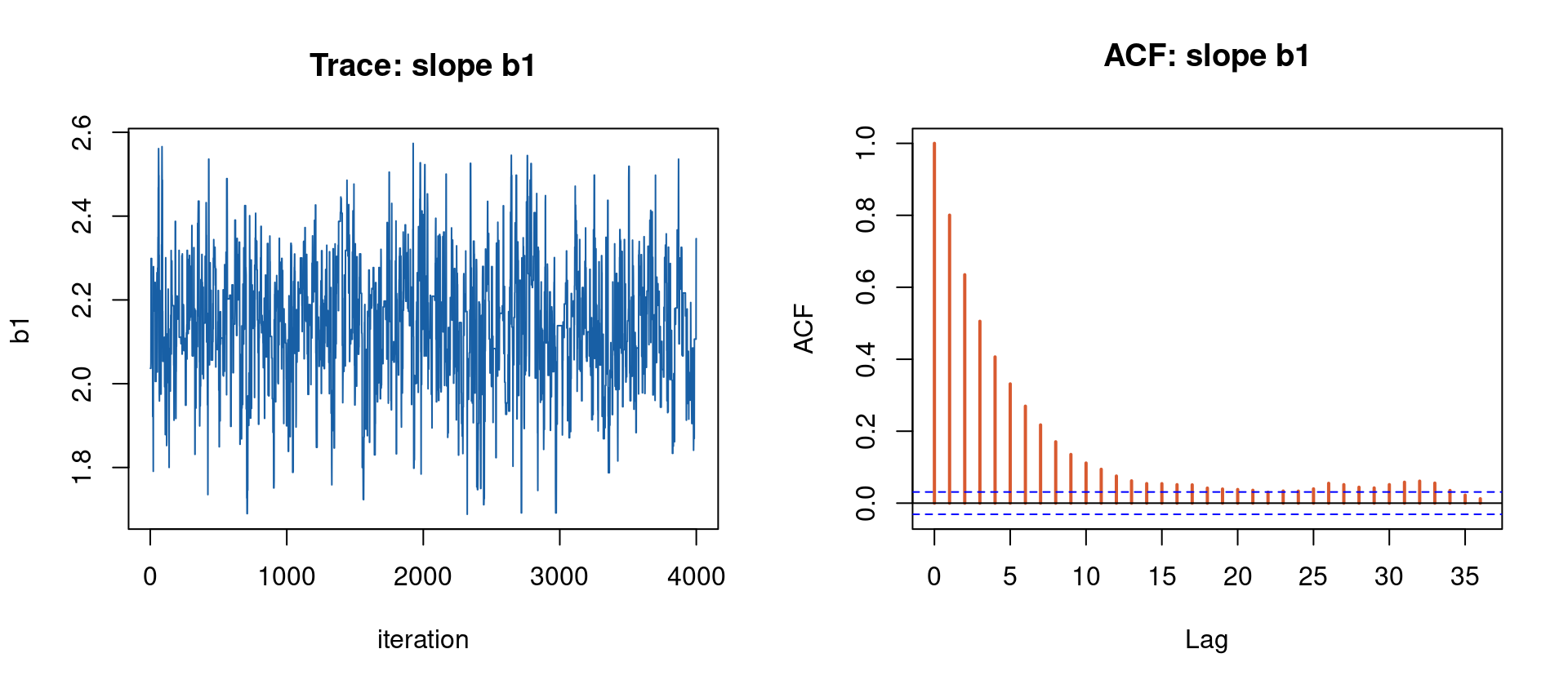
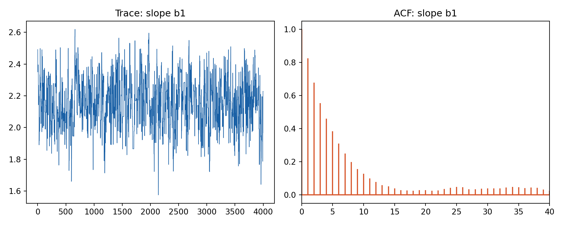
• Gibbs on this conjugate model produces near-independent draws (ESS close to the number of iterations)
• Random-walk MH produces correlated draws — the ACF decays slowly, ESS is a fraction of the raw count
• That gap is exactly what Hamiltonian Monte Carlo (Part III) is built to close
• Always report ESS and \(\hat R\) next to every posterior number — they are the MCMC analogue of a standard error

Turn ESS into a Monte Carlo error bar

The Monte Carlo standard error of a posterior mean is \[ \text{MCSE} \;=\; \frac{\widehat{\text{sd}}(\theta)}{\sqrt{\text{ESS}}}. \] Report it so readers know how many significant digits of your posterior mean are actually resolved. Rule of thumb: sample until MCSE is an order of magnitude smaller than the posterior sd you care about — ESS \(\gtrsim 100\) for a mean, and considerably more for tail quantiles such as a 97.5% credible bound.

Metropolis-within-Gibbs

• When One Block Refuses

Gibbs needs every full conditional in closed form. Change one prior and that breaks. Put a half-Cauchy prior on the error scale — the modern default for scale parameters, because it is flat near zero and heavy-tailed:

\[ \sigma \sim \mathcal{C}^{+}(0, 1), \qquad p(\sigma) = \frac{2}{\pi\,(1 + \sigma^2)}, \quad \sigma > 0 \]

Now \(p(\sigma \mid \beta, y)\) is not an inverse-gamma. The fix is not to abandon Gibbs but to replace the offending block with a Metropolis step:

• \(\beta \mid \sigma^2, y\) — still Normal, draw it exactly
• \(\sigma \mid \beta, y\) — no closed form, take one Metropolis step

The result is a valid Markov chain with the right stationary distribution: each block leaves \(p(\theta\mid y)\) invariant, so their composition does too. We sample \(\ell = \log\sigma\) so the proposal is unconstrained, which adds the Jacobian \(\sigma\):

\[ \log p(\ell \mid \beta, y) = -n\ell - \frac{\sum_i \varepsilon_i^2}{2 e^{2\ell}} + \log p(e^{\ell}) + \ell \]

d <- read.csv("../data/bayes-linreg.csv")
X <- cbind(1, d$x); y <- d$y; n <- nrow(X)
XtX <- crossprod(X); Xty <- crossprod(X, y)

# log posterior of log-sigma given beta: half-Cauchy prior plus Jacobian
log_ls <- function(ls, b) {
  s2 <- exp(2 * ls); r <- y - X %*% b
  -n * ls - sum(r^2) / (2 * s2) - log1p(exp(2 * ls)) + ls
}

set.seed(14159)
S <- 8000; b <- c(0, 0); ls <- 0; keep <- matrix(NA, S, 3); acc <- 0
for (t in 1:S) {
  s2 <- exp(2 * ls)
  Vb <- solve(diag(1 / 100, 2) + XtX / s2)          # Gibbs block: beta
  b  <- as.vector(mvrnorm(1, Vb %*% (Xty / s2), Vb))
  prop <- ls + rnorm(1, 0, 0.09)                    # Metropolis block: log sigma
  if (log(runif(1)) < log_ls(prop, b) - log_ls(ls, b)) { ls <- prop; acc <- acc + 1 }
  keep[t, ] <- c(b, exp(ls))
}
kp <- keep[2001:S, ]
cat(sprintf("MH acceptance for sigma = %.2f\n", acc / S))
cat(sprintf("b0 = %.3f   b1 = %.3f   sigma = %.3f\n",
            mean(kp[, 1]), mean(kp[, 2]), mean(kp[, 3])))

MH acceptance for sigma = 0.61

b0 (true 1.0) = 0.785   b1 (true 2.0) = 2.140   sigma (true 1.5) = 1.600

The conjugate inverse-gamma run in Part II gave sigma = 1.60 as well:

with 120 observations the likelihood dominates and the prior swap barely registers.

import numpy as np, pandas as pd

d = pd.read_csv("../data/bayes-linreg.csv")
X = np.column_stack([np.ones(len(d)), d["x"].values]); y = d["y"].values; n = len(y)
XtX = X.T @ X; Xty = X.T @ y

def log_ls(ls, b):                      # half-Cauchy prior plus Jacobian
    s2 = np.exp(2 * ls); r = y - X @ b
    return -n * ls - r @ r / (2 * s2) - np.log1p(np.exp(2 * ls)) + ls

rng = np.random.default_rng(14159)
S = 8000; b = np.zeros(2); ls = 0.0; keep = np.empty((S, 3)); acc = 0
for t in range(S):
    s2 = np.exp(2 * ls)
    Vb = np.linalg.inv(np.diag([1/100, 1/100]) + XtX / s2)   # Gibbs block
    b = rng.multivariate_normal(Vb @ (Xty / s2), Vb)
    prop = ls + rng.normal(0, 0.09)                          # Metropolis block
    if np.log(rng.uniform()) < log_ls(prop, b) - log_ls(ls, b):
        ls, acc = prop, acc + 1
    keep[t] = [b[0], b[1], np.exp(ls)]

kp = keep[2000:]
out = (f"MH acceptance for sigma = {acc/S:.2f}\n"
       f"b0 (true 1.0) = {kp[:,0].mean():.3f}   b1 (true 2.0) = {kp[:,1].mean():.3f}   "
       f"sigma (true 1.5) = {kp[:,2].mean():.3f}")
import sys; sys.stdout.write(out + "\n"); sys.stdout.flush()

MH acceptance for sigma = 0.61
b0 (true 1.0) = 0.786   b1 (true 2.0) = 2.144   sigma (true 1.5) = 1.600
104

set linesize 255
quietly import delimited "../data/bayes-linreg.csv", clear
quietly destring _all, replace
* block() puts sigma in its own Metropolis block: this is Metropolis-within-Gibbs.
* logdensity() supplies the half-Cauchy prior Stata has no built-in name for.
bayesmh y x, likelihood(normal({sig}^2)) prior({y:x _cons}, normal(0, 100)) prior({sig}, logdensity(cond({sig}>0, log(2/(_pi*(1+{sig}^2))), -1e10))) block({sig}) initial({y:x} 2 {y:_cons} 1 {sig} 1.5) rseed(14159) nomodelsummary mcmcsize(8000) burnin(2000)

Burn-in ...
Simulation ...

Bayesian normal regression                       MCMC iterations  =     10,000
Random-walk Metropolis–Hastings sampling         Burn-in          =      2,000
                                                 MCMC sample size =      8,000
                                                 Number of obs    =        120
                                                 Acceptance rate  =      .3207
                                                 Efficiency:  min =     .08577
                                                              avg =       .145
Log marginal-likelihood = -236.74711                          max =      .2223

------------------------------------------------------------------------------
             |                                                Equal-tailed
             |      Mean   Std. dev.     MCSE     Median  [95% cred. interval]
-------------+----------------------------------------------------------------
y            |
           x |  2.140352   .1506602   .005752   2.137209   1.839801   2.451746
       _cons |  .7824409   .1420346   .004455   .7821245   .4886489   1.055775
-------------+----------------------------------------------------------------
         sig |  1.596801   .1034445   .002453    1.59298   1.410188   1.811357
------------------------------------------------------------------------------
Note: Adaptation continues during simulation.

Data Augmentation — Albert–Chib Probit

• The Trick
• DGP

The probit likelihood has no conjugate prior — but it is a censored linear model in disguise. Reintroduce the latent utility that generated the binary outcome:

\[ z_i = x_i'\beta + \varepsilon_i, \quad \varepsilon_i\sim\mathcal{N}(0,1), \qquad y_i = \mathbb{1}\{z_i > 0\} \]

Treat \(z\) as a missing variable and sample it alongside \(\beta\). Both full conditionals are then standard (Albert & Chib 1993):

\[ z_i \mid \beta, y_i \sim \begin{cases} \mathcal{TN}_{(0,\infty)}(x_i'\beta,\, 1) & y_i = 1 \\[2pt] \mathcal{TN}_{(-\infty,0)}(x_i'\beta,\, 1) & y_i = 0 \end{cases} \]

\[ \beta \mid z \sim \mathcal{N}\big( (V_0^{-1} + X'X)^{-1} X'z,\ (V_0^{-1} + X'X)^{-1} \big) \]

The variance is fixed at 1 — the probit scale is not identified — so the \(\beta\) block is the ordinary conjugate regression draw. The same device extends to ordered probit and to Tobit, where \(z\) is censored rather than dichotomised.

# This block lives in bayesian-computation-data.R, run once before rendering.
set.seed(14159)
n <- 600; b0 <- -0.3; b1 <- 0.8; b2 <- -0.5
x1 <- rnorm(n); x2 <- rnorm(n)
ystar <- b0 + b1 * x1 + b2 * x2 + rnorm(n)
y <- as.numeric(ystar > 0)
write.csv(data.frame(y = y, x1 = x1, x2 = x2),
          "../data/bayes-probit.csv", row.names = FALSE)

p <- read.csv("../data/bayes-probit.csv")
X <- cbind(1, p$x1, p$x2); y <- p$y; n <- nrow(X)
Vb <- solve(diag(1 / 100, 3) + crossprod(X))     # fixed: latent variance is 1

set.seed(14159)
S <- 6000; b <- c(0, 0, 0); keep <- matrix(NA, S, 3)
for (t in 1:S) {
  mu <- as.vector(X %*% b)
  lo <- ifelse(y == 1, pnorm(-mu), 0)            # truncated normal by inverse CDF
  hi <- ifelse(y == 1, 1, pnorm(-mu))
  z  <- mu + qnorm(runif(n, lo, hi))
  b  <- as.vector(mvrnorm(1, Vb %*% crossprod(X, z), Vb))
  keep[t, ] <- b
}
kb <- keep[1001:S, ]
cat(sprintf("b0 = %6.3f  b1 = %6.3f  b2 = %6.3f\n",
            mean(kb[, 1]), mean(kb[, 2]), mean(kb[, 3])))

Gibbs : b0 (true -0.3) = -0.264  b1 (true 0.8) =  0.786  b2 (true -0.5) = -0.488

MLE   : b0 = -0.263  b1 =  0.780  b2 = -0.485   (agreement to three decimals)

import numpy as np, pandas as pd
from scipy import stats

p = pd.read_csv("../data/bayes-probit.csv")
X = np.column_stack([np.ones(len(p)), p["x1"].values, p["x2"].values])
y = p["y"].values
Vb = np.linalg.inv(np.diag([1/100]*3) + X.T @ X)

rng = np.random.default_rng(14159)
S = 6000; b = np.zeros(3); keep = np.empty((S, 3))
for t in range(S):
    mu = X @ b
    lo = np.where(y == 1, -mu, -np.inf)          # scipy truncates in standard units
    hi = np.where(y == 1, np.inf, -mu)
    z = mu + stats.truncnorm.rvs(lo, hi, random_state=rng)
    b = rng.multivariate_normal(Vb @ (X.T @ z), Vb)
    keep[t] = b

kb = keep[1000:]
out = (f"Gibbs : b0 (true -0.3) = {kb[:,0].mean():6.3f}  "
       f"b1 (true 0.8) = {kb[:,1].mean():6.3f}  b2 (true -0.5) = {kb[:,2].mean():6.3f}")
import sys; sys.stdout.write(out + "\n"); sys.stdout.flush()

Gibbs : b0 (true -0.3) = -0.265  b1 (true 0.8) =  0.790  b2 (true -0.5) = -0.489
81

Probit — Production Cross-Checks

• Same Posterior, Three Engines
• brms
• PyMC

The hand-coded sampler is not a toy: every production tool below targets the same posterior, and all four agree to two decimals. What differs is the machinery — data augmentation with Gibbs, NUTS on the marginal likelihood, or adaptive Metropolis–Hastings.

• brms writes Stan code and runs NUTS on the probit likelihood directly, without latent \(z\)
• PyMC does the same through its own NUTS implementation
• Stata’s bayes: prefix uses adaptive Metropolis–Hastings, again with no augmentation

Agreement across three different algorithms is the strongest evidence that the hand-coded chain has converged to the right target.

library(brms)
p <- read.csv("../data/bayes-probit.csv")
fit <- brm(y ~ x1 + x2, data = p, family = bernoulli(link = "probit"),
           prior = prior(normal(0, 10), class = b),
           chains = 2, iter = 2000, warmup = 1000, seed = 14159, refresh = 0)
fixef(fit)

brms -- NUTS on the probit likelihood (no latent z):

          Estimate Est.Error   Q2.5  Q97.5
Intercept   -0.261     0.060 -0.376 -0.142
x1           0.783     0.073  0.642  0.924
x2          -0.489     0.065 -0.618 -0.367

import warnings; warnings.filterwarnings("ignore")
import numpy as np, pandas as pd, pymc as pm, arviz as az

p = pd.read_csv("../data/bayes-probit.csv")
with pm.Model():
    b = pm.Normal("b", 0, 10, shape=3)
    eta = b[0] + b[1] * p["x1"].values + b[2] * p["x2"].values
    pm.Bernoulli("y", p=pm.math.invprobit(eta), observed=p["y"].values)
    idata = pm.sample(1000, tune=1000, chains=2, random_seed=14159, progressbar=False)

y

su = az.summary(idata, var_names=["b"])[["mean", "hdi_3%", "hdi_97%"]].round(3)
out = "PyMC -- NUTS through the inverse probit link:\n" + su.to_string()
import sys; sys.stdout.write(out + "\n"); sys.stdout.flush()

PyMC -- NUTS through the inverse probit link:
       mean  hdi_3%  hdi_97%
b[0] -0.264  -0.375   -0.151
b[1]  0.782   0.648    0.925
b[2] -0.489  -0.606   -0.369
162

set linesize 255
quietly import delimited "../data/bayes-probit.csv", clear
quietly destring _all, replace
bayes, prior({y:x1 x2 _cons}, normal(0, 100)) rseed(14159) nomodelsummary mcmcsize(6000) burnin(1000): probit y x1 x2

Burn-in ...
Simulation ...

Bayesian probit regression                       MCMC iterations  =      7,000
Random-walk Metropolis–Hastings sampling         Burn-in          =      1,000
                                                 MCMC sample size =      6,000
                                                 Number of obs    =        600
                                                 Acceptance rate  =      .2218
                                                 Efficiency:  min =     .07544
                                                              avg =     .08547
Log marginal-likelihood = -318.09486                          max =      .0988

------------------------------------------------------------------------------
             |                                                Equal-tailed
           y |      Mean   Std. dev.     MCSE     Median  [95% cred. interval]
-------------+----------------------------------------------------------------
          x1 |  .7861096   .0704137   .003171   .7868829   .6508006   .9237641
          x2 | -.4860932   .0627755   .002951  -.4832615  -.6135965  -.3607903
       _cons | -.2644775   .0596797   .002451  -.2628735  -.3829122  -.1510817
------------------------------------------------------------------------------

Part III: Hamiltonian Monte Carlo

Using gradients and physics to beat the random walk

Hamiltonian Monte Carlo

• Physics as a Proposal
• The Leapfrog Integrator
• NUTS and the Real World

A random walk explores by diffusion — it takes \(O(d^2)\) steps to cross a \(d\)-dimensional posterior. HMC instead rolls a ball across the landscape, using the gradient to make long, informed moves. Introduce a momentum \(r\) and define energy

\[ H(\theta, r) \;=\; \underbrace{-\log p(\theta\mid y)}_{\text{potential } U(\theta)} \;+\; \underbrace{\tfrac12 r'M^{-1}r}_{\text{kinetic } K(r)} \]

Simulating Hamilton’s equations conserves \(H\), so a proposal far away is still accepted with high probability. The gradient \(\nabla_\theta \log p(\theta\mid y)\) is what makes this possible.

Hamilton’s equations are discretised by the leapfrog scheme, which is reversible and volume-preserving — both required for a valid MCMC proposal:

\[ r_{t+\epsilon/2} = r_t - \tfrac{\epsilon}{2}\nabla U(\theta_t), \quad \theta_{t+\epsilon} = \theta_t + \epsilon\, r_{t+\epsilon/2}, \quad r_{t+\epsilon} = r_{t+\epsilon/2} - \tfrac{\epsilon}{2}\nabla U(\theta_{t+\epsilon}) \]

Run \(L\) leapfrog steps of size \(\epsilon\), then accept the endpoint with

\[ \alpha = \min\Big\{1,\; \exp\!\big(H(\theta, r) - H(\theta^\star, r^\star)\big)\Big\} \]

Discretisation error is corrected by this Metropolis step, so HMC is exact, not approximate.

• Two knobs — step size \(\epsilon\) and path length \(L\) — are hard to tune by hand
• The No-U-Turn Sampler (Hoffman & Gelman 2014) picks \(L\) automatically by running the trajectory until it doubles back, and adapts \(\epsilon\) during warm-up
• NUTS is the default engine of Stan, PyMC and brms
• HMC needs a differentiable log posterior; discrete parameters must be marginalised out
• Payoff: near-independent draws even in hundreds of dimensions — decisive for DSGE and large hierarchical models

HMC vs Random Walk — Same Posterior

• The Experiment
• by hand
• by hand
• Stan
• PyMC
• Takeaway

We sample the same linear-model posterior as Part II, now with hand-coded HMC (\(\epsilon = 0.015\), \(L = 25\)), and compare effective sample size against random-walk Metropolis. The gradient of \(U(\theta) = -\log p(\theta\mid y)\) is analytic:

\[ \nabla_\beta U = -\frac{X'(y - X\beta)}{\sigma^2} + \frac{\beta}{100}, \qquad \frac{\partial U}{\partial \ell} = n - \frac{\sum_i \varepsilon_i^2}{\sigma^2} + \frac{\ell}{25} \]

The prize is effective sample size per iteration: HMC turns correlated draws into nearly independent ones.

Do not be alarmed when the reported ESS exceeds the number of draws. With \(\text{ESS} = S/(1 + 2\sum_k \rho_k)\), successive HMC draws can be negatively autocorrelated, so \(\sum_k \rho_k < 0\) and the ratio rises above \(S\) — antithetic behaviour that beats independent sampling, not a bug.

d <- read.csv("../data/bayes-linreg.csv")
X <- cbind(1, d$x); y <- d$y; n <- nrow(X)

U <- function(q) {                    # potential = -log posterior
  b <- q[1:2]; l <- q[3]; s2 <- exp(2 * l); r <- y - X %*% b
  -(-n * l - sum(r^2) / (2 * s2) + sum(dnorm(b, 0, 10, log = TRUE)) + dnorm(l, 0, 5, log = TRUE))
}
grad_U <- function(q) {
  b <- q[1:2]; l <- q[3]; s2 <- exp(2 * l); r <- y - X %*% b
  gb <- -as.vector(crossprod(X, r)) / s2 + b / 100
  gl <- n - sum(r^2) / s2 + l / 25
  c(gb, gl)
}

hmc_step <- function(q, eps, L) {
  r0 <- rnorm(length(q)); q0 <- q; r <- r0
  r <- r - 0.5 * eps * grad_U(q)
  for (i in 1:L) { q <- q + eps * r; if (i < L) r <- r - eps * grad_U(q) }
  r <- r - 0.5 * eps * grad_U(q)
  H0 <- U(q0) + 0.5 * sum(r0^2); H1 <- U(q) + 0.5 * sum(r^2)
  if (log(runif(1)) < H0 - H1) list(q = q, acc = 1) else list(q = q0, acc = 0)
}

set.seed(14159)
S <- 3000; chain <- matrix(NA, S, 3); q <- c(0, 0, 0); acc <- 0
for (t in 1:S) { out <- hmc_step(q, 0.015, 25); q <- out$q; acc <- acc + out$acc; chain[t, ] <- q }

keep <- chain[501:S, ]
cat(sprintf("HMC acceptance = %.2f   ESS(b1) = %.0f of %d draws\n",
            acc / S, coda::effectiveSize(keep[, 2]), nrow(keep)))

HMC : acceptance = 1.00   posterior mean b1 = 2.141

HMC ESS(b1)      = 19780 of 2500 draws

RW-MH ESS(b1)    = 443 of 4000 draws  -> HMC is far more efficient per draw

import numpy as np, pandas as pd

d = pd.read_csv("../data/bayes-linreg.csv")
X = np.column_stack([np.ones(len(d)), d["x"].values]); y = d["y"].values; n = len(y)

def U(q):
    b, l = q[:2], q[2]; s2 = np.exp(2 * l); r = y - X @ b
    return -(-n * l - r @ r / (2 * s2) - (b @ b) / 200 - l**2 / 50)
def grad_U(q):
    b, l = q[:2], q[2]; s2 = np.exp(2 * l); r = y - X @ b
    gb = -(X.T @ r) / s2 + b / 100
    gl = n - r @ r / s2 + l / 25
    return np.append(gb, gl)

def hmc_step(q, eps, L, rng):
    r0 = rng.standard_normal(len(q)); q0 = q.copy(); r = r0.copy()
    r -= 0.5 * eps * grad_U(q)
    for i in range(L):
        q = q + eps * r
        if i < L - 1: r -= eps * grad_U(q)
    r -= 0.5 * eps * grad_U(q)
    H0 = U(q0) + 0.5 * r0 @ r0; H1 = U(q) + 0.5 * r @ r
    return (q, 1) if np.log(rng.uniform()) < H0 - H1 else (q0, 0)

rng = np.random.default_rng(14159)
S = 3000; chain = np.empty((S, 3)); q = np.zeros(3); acc = 0
for t in range(S):
    q, a = hmc_step(q, 0.015, 25, rng); acc += a; chain[t] = q
keep = chain[500:]
print(f"HMC acceptance = {acc/S:.2f}   posterior mean b1 = {keep[:,1].mean():.3f}")

HMC acceptance = 1.00   posterior mean b1 = 2.141

library(rstan)
d <- read.csv("../data/bayes-linreg.csv")

sc <- "
data { int<lower=0> N; vector[N] x; vector[N] y; }
parameters { real b0; real b1; real<lower=0> sigma; }
model { b0 ~ normal(0, 10); b1 ~ normal(0, 10); sigma ~ normal(0, 5);
        y ~ normal(b0 + b1 * x, sigma); }
"
# Stan runs adaptive HMC (NUTS): it tunes step size and path length for us.
# iter = 2000 => 1000 warmup + 1000 kept draws per chain (2000 total).
fit <- stan(model_code = sc, data = list(N = nrow(d), x = d$x, y = d$y),
            chains = 2, iter = 2000, warmup = 1000, seed = 14159, refresh = 0)
print(fit, pars = c("b0", "b1", "sigma"))       # mean, n_eff and Rhat

Stan NUTS — 2 chains x 1000 post-warmup draws (2000 total):

       mean  2.5% 97.5%    n_eff
b0    0.786 0.494 1.078 2566.405
b1    2.145 1.834 2.435 2059.989
sigma 1.616 1.424 1.839 2285.242

NUTS ESS(b1) = 2060 of 2000 draws — near-independent, matching hand-coded HMC

import warnings; warnings.filterwarnings("ignore")
import numpy as np, pandas as pd, pymc as pm, arviz as az

d = pd.read_csv("../data/bayes-linreg.csv")
with pm.Model() as model:
    b0 = pm.Normal("b0", 0, 10); b1 = pm.Normal("b1", 0, 10)
    sigma = pm.HalfNormal("sigma", 5)
    pm.Normal("y", b0 + b1 * d["x"].values, sigma, observed=d["y"].values)
    # draws=1000, tune=1000 warmup, 2 chains => 2000 kept draws
    idata = pm.sample(1000, tune=1000, chains=2, random_seed=14159,
                      progressbar=False, target_accept=0.9)      # NUTS

y

su = az.summary(idata, var_names=["b0", "b1", "sigma"])
print(su[["mean", "hdi_3%", "hdi_97%", "ess_bulk"]].round(3))

        mean  hdi_3%  hdi_97%  ess_bulk
b0     0.784   0.535    1.084    1475.0
b1     2.139   1.856    2.449    2082.0
sigma  1.612   1.423    1.806    2054.0

print(f"NUTS ESS(b1) = {su.loc['b1','ess_bulk']:.0f} of 2000 draws")

NUTS ESS(b1) = 2082 of 2000 draws

• Both samplers hit the same posterior mean — HMC does not change the answer
• HMC’s edge is statistical efficiency: many more effective draws per iteration, so tighter Monte Carlo error for the same run length
• The cost is one gradient evaluation per leapfrog step — cheap here, automated by autodiff in Stan/PyMC for models with no hand-derived gradient
• In the 3-parameter toy the gap is modest; in a 200-parameter hierarchical or DSGE posterior it is the difference between feasible and hopeless

Stan & PyMC — Functions, Tuning, Internals

• Why these tools
• The calls
• Parameter tuning
• Under the hood

We hand-code the samplers to see the mechanics; for real models we hand the same posterior to Stan (rstan, brms) or PyMC, which implement NUTS — adaptive Hamiltonian Monte Carlo.

• Pros: near-independent draws, scales to hundreds of parameters, gradients built by automatic differentiation, and \(\hat R\)/ESS/divergence diagnostics reported for free
• Cons: parameters must be continuous and differentiable (discrete ones marginalised out); Stan compiles C++ once (~30–60 s); stiff geometries (funnels) need tuning
• Why right here: the linear, hierarchical and DSGE posteriors are smooth and continuous — exactly HMC’s home ground. Conjugate Gibbs also works but does not generalise beyond conjugacy, whereas NUTS handles any differentiable likelihood

• rstan: stan_model(model_code=) compiles the C++ once; then sampling(sm, data=, chains=, iter=, warmup=, seed=). Read results from summary(fit)$summary (posterior mean, n_eff, Rhat)
• brms: brm(formula, data, family=, prior=, chains=, iter=) writes and compiles the Stan program for you — inspect it with make_stancode(), set priors via prior(), list them with get_prior()
• PyMC: declare the model in a with pm.Model(): block, then pm.sample(draws, tune=, chains=, target_accept=); summarise with arviz.summary()
• All three read R’s shared CSV — no binary interchange formats

• chains — run 2–4 from dispersed starts so \(\hat R\) can compare them
• warmup / tune — adaptation draws, discarded; only iter − warmup are kept
• adapt_delta (Stan/brms) / target_accept (PyMC) — target acceptance, default 0.8; raise to 0.95–0.99 to kill divergences, at the price of smaller steps
• max_treedepth — cap on the NUTS trajectory doubling (default 10); hitting it flags a hard posterior
• seed / random_seed, cores — reproducibility and one chain per core

Divergences are not optional to read

A divergent transition means the leapfrog integrator blew up where the posterior is sharply curved — those draws are biased and must not be ignored. First raise adapt_delta / target_accept toward 0.99 (smaller steps). If they persist, the geometry is the problem: reparameterise — e.g. the non-centred form \[ \alpha_j = \mu + \tau\, z_j, \qquad z_j \sim \mathcal{N}(0, 1) \] for hierarchical funnels. Stan and PyMC report the divergence count right next to \(\hat R\) and ESS — check it every run.

• NUTS extends HMC by growing the leapfrog trajectory until it doubles back — so you never hand-set the path length \(L\) of Part III
• Warmup runs dual averaging (Nesterov) to tune the step size \(\epsilon\) to the target acceptance, and estimates a diagonal mass matrix (the metric) from the warmup draws
• Gradients \(\nabla\log p(\theta\mid y)\) come from reverse-mode automatic differentiation — Stan Math in rstan/brms, PyTensor in PyMC — never derived by hand
• Point modes use quasi-Newton L-BFGS: rstan::optimizing() for the MAP, pm.find_MAP() (SciPy L-BFGS-B); fast approximate posteriors use ADVI variational inference
• Initialisation: Stan draws random unconstrained starts in \((-2, 2)\); PyMC uses jitter+adapt_diag

Neal’s Funnel — Geometry Beats Tuning

• The Pathology
• The Fix
• Stan
• PyMC

Hierarchical models hide a hard geometry. Neal’s funnel is the distilled version:

\[ v \sim \mathcal{N}(0, 3^2), \qquad x_j \mid v \sim \mathcal{N}\big(0,\, e^{v/2}\big), \quad j = 1,\dots,9 \]

The conditional scale of \(x\) depends on \(v\), so the joint density is a funnel: wide and flat at large \(v\), pinched into a narrow neck as \(v \to -\infty\). No single HMC step size works — a step tuned for the mouth overshoots the neck, a step tuned for the neck crawls through the mouth.

The symptom is divergent transitions: the leapfrog integrator becomes unstable, energy is not conserved, and the sampler reports the failure rather than hiding it.

Rewrite the model so the parameters are a priori independent and the dependence is moved into a deterministic transformation:

\[ z_j \sim \mathcal{N}(0, 1), \qquad x_j = e^{v/2}\, z_j \]

This is the non-centred parameterisation. The sampler now explores \((v, z)\), whose joint density is a spherical Gaussian — no neck, one step size fits everywhere. The quantity of interest \(x_j\) is recovered afterwards by the transformation, so nothing is lost.

Watch three diagnostics, not one: divergences, ESS, and whether the marginal \(\text{sd}(v)\) recovers its known value of 3.

library(rstan)
sc_centred <- "
parameters { real v; vector[9] x; }
model { v ~ normal(0, 3); x ~ normal(0, exp(v/2)); }
"
sc_noncentred <- "
parameters { real v; vector[9] z; }
transformed parameters { vector[9] x = exp(v/2) * z; }
model { v ~ normal(0, 3); z ~ std_normal(); }
"
for (nm in c("centred", "non-centred")) {
  code <- if (nm == "centred") sc_centred else sc_noncentred
  fit <- stan(model_code = code, chains = 2, iter = 2000, warmup = 1000,
              seed = 14159, refresh = 0)
  sp  <- get_sampler_params(fit, inc_warmup = FALSE)
  div <- sum(sapply(sp, function(z) sum(z[, "divergent__"])))
  cat(sprintf("%-12s divergences = %4d   ESS(v) = %6.0f   sd(v) = %.2f\n",
              nm, div, summary(fit, pars = "v")$summary[, "n_eff"],
              sd(extract(fit, "v")$v)))
}

centred      divergences =    2 of 2000   ESS(v) =     28   sd(v) = 2.28
non-centred  divergences =    0 of 2000   ESS(v) =   3849   sd(v) = 2.93

truth: v ~ N(0, 3^2), so sd(v) = 3.00

The centred run is not merely slower: its marginal sd of v is biased low,

because the chain never reaches the neck of the funnel.

import warnings; warnings.filterwarnings("ignore")
import numpy as np, pymc as pm, arviz as az

def run(centred):
    with pm.Model():
        v = pm.Normal("v", 0, 3)
        if centred:
            pm.Normal("x", 0, pm.math.exp(v / 2), shape=9)
        else:
            z = pm.Normal("z", 0, 1, shape=9)
            pm.Deterministic("x", pm.math.exp(v / 2) * z)
        return pm.sample(1000, tune=1000, chains=2, random_seed=14159,
                         progressbar=False, target_accept=0.8)

lines = []
for nm, c in (("centred", True), ("non-centred", False)):
    idata = run(c)
    div = int(idata.sample_stats["diverging"].sum())
    ess = float(az.ess(idata, var_names=["v"])["v"])
    lines.append(f"{nm:12} divergences = {div:4d} of 2000   ESS(v) = {ess:6.0f}   "
                 f"sd(v) = {float(idata.posterior['v'].std()):.2f}")
lines.append("truth: v ~ N(0, 3^2), so sd(v) = 3.00")
out = "\n".join(lines)
import sys; sys.stdout.write(out + "\n"); sys.stdout.flush()

centred      divergences =    0 of 2000   ESS(v) =      7   sd(v) = 2.73
non-centred  divergences =    0 of 2000   ESS(v) =   2246   sd(v) = 3.06
truth: v ~ N(0, 3^2), so sd(v) = 3.00
184

Centred or Non-Centred? It Depends on the Data

• No Universal Winner
• Reading It

It is tempting to take “always use non-centred” from the funnel slide. That is wrong, and the reason is instructive.

The funnel geometry appears only when the likelihood is weak relative to the hierarchical prior — when each group has few observations, so \(\alpha_j\) is pinned by \(\tau\) rather than by its own data. Then the prior dependence dominates and the non-centred form wins.

When groups are informative, the likelihood breaks the prior dependence by itself. The centred parameterisation is then the better-conditioned one, and the non-centred rewrite actually introduces correlation between \(\tau\) and \(z\).

\[ \text{centred: } \alpha_j \sim \mathcal{N}(\mu, \tau^2) \qquad\text{vs}\qquad \text{non-centred: } \alpha_j = \mu + \tau z_j,\ z_j\sim\mathcal{N}(0,1) \]

We fit the Part VII panel both ways, at \(n_j = 8\) observations per group and again thinned to \(n_j = 2\).

import warnings; warnings.filterwarnings("ignore")
import numpy as np, pandas as pd, pymc as pm, arviz as az

full = pd.read_csv("../data/bayes-panel.csv")
thin = full.groupby("group").head(2).reset_index(drop=True)     # weak-likelihood version

def run(d, centred):
    g = d["group"].values - 1; J = int(d["group"].max())
    with pm.Model():
        mu = pm.Normal("mu", 0, 10); tau = pm.HalfNormal("tau", 10)
        a = (pm.Normal("a", mu, tau, shape=J) if centred
             else pm.Deterministic("a", mu + tau * pm.Normal("z", 0, 1, shape=J)))
        beta = pm.Normal("beta", 0, 10); sig = pm.HalfNormal("sig", 10)
        pm.Normal("y", a[g] + beta * d["x"].values, sig, observed=d["y"].values)
        return pm.sample(1000, tune=1000, chains=2, random_seed=14159,
                         progressbar=False, target_accept=0.8)

lines = []
for lbl, d in (("n_j = 8 (informative)", full), ("n_j = 2 (weak)", thin)):
    for nm, c in (("centred", True), ("non-centred", False)):
        i = run(d, c)
        lines.append(f"{lbl:22} {nm:12} divergences = {int(i.sample_stats['diverging'].sum()):3d}"
                     f"   ESS(tau) = {float(az.ess(i, var_names=['tau'])['tau']):6.0f}"
                     f"   tau = {float(i.posterior['tau'].mean()):.2f}")
lines.append("With 8 observations per group the centred form is far more efficient;")
lines.append("thinned to 2, it starts diverging and the non-centred form takes over.")
out = "\n".join(lines)
import sys; sys.stdout.write(out + "\n"); sys.stdout.flush()

n_j = 8 (informative)  centred      divergences =   0   ESS(tau) =   2892   tau = 1.06
n_j = 8 (informative)  non-centred  divergences =   0   ESS(tau) =    435   tau = 1.06
n_j = 2 (weak)         centred      divergences =   7   ESS(tau) =     90   tau = 0.79
n_j = 2 (weak)         non-centred  divergences =   2   ESS(tau) =    349   tau = 0.74
With 8 observations per group the centred form is far more efficient;
thinned to 2, it starts diverging and the non-centred form takes over.
489

set linesize 255
quietly import delimited "../data/bayes-panel.csv", clear
quietly destring _all, replace
* Stata samples this model with adaptive Metropolis-Hastings, not HMC, so it
* reports efficiency rather than divergences, and exposes no centring switch.
bayes, rseed(14159) nomodelsummary: mixed y x || group:

note: Gibbs sampling is used for regression coefficients and variance components.

Burn-in 2500 aaaaaaaaa1000aaaaaaaaa2000aaaaa done
Simulation 10000 .........1000.........2000.........3000.........4000.........5000.........6000.........7000.........8000.........9000.........10000 done

Multilevel structure
------------------------------------------------------------------------------
group
    {U0}: random intercepts
------------------------------------------------------------------------------

Bayesian multilevel regression                   MCMC iterations  =     12,500
Metropolis–Hastings and Gibbs sampling           Burn-in          =      2,500
                                                 MCMC sample size =     10,000
Group variable: group                            Number of groups =         20
                                                 Obs per group:
                                                              min =          8
                                                              avg =        8.0
                                                              max =          8
                                                 Number of obs    =        160
                                                 Acceptance rate  =      .8222
                                                 Efficiency:  min =     .01487
                                                              avg =      .3186
Log marginal-likelihood                                       max =      .5829

------------------------------------------------------------------------------
             |                                                Equal-tailed
             |      Mean   Std. dev.     MCSE     Median  [95% cred. interval]
-------------+----------------------------------------------------------------
y            |
           x |  .8645687    .087844   .001151   .8638244   .6913786   1.037076
       _cons |  1.042984   .2534011    .02078   1.040071   .5464203   1.553284
-------------+----------------------------------------------------------------
group        |
   U0:sigma2 |  1.104238   .4509203   .011831   1.016022   .5092272   2.257215
-------------+----------------------------------------------------------------
e.y          |
      sigma2 |  1.045972   .1283635   .001761    1.03391   .8258246   1.332342
------------------------------------------------------------------------------
Note: Default priors are used for model parameters.

• Divergences are an HMC diagnostic: they come from the leapfrog integrator, so Stan and PyMC report them and Stata’s Metropolis–Hastings sampler does not
• A parameterisation is not “correct” or “incorrect” — the two define the same posterior and differ only in how easy that posterior is to traverse
• The practical rule: start centred, and switch when divergences or a collapsed ESS say the likelihood is too weak to break the funnel
• brms and rstanarm default to the non-centred form for group effects, which is why hierarchical fits there rarely diverge

Part IV: Priors

Elicitation, weak information, and honest sensitivity analysis

Choosing and Checking Priors

• A Spectrum of Priors
• Prior Predictive Checks
• Sensitivity Analysis

The prior is a modelling choice, not a nuisance to hide. The useful distinctions:

• Conjugate: analytically convenient (Beta–Binomial, Normal–Inverse-Gamma) — great for teaching and Gibbs
• Weakly-informative: rule out absurd values, let the data drive — e.g. \(\beta\sim\mathcal{N}(0, 2.5^2)\) on standardised predictors, \(\sigma\sim\text{Half-Cauchy}(0,1)\)
• Informative: genuine external knowledge — an elasticity in \([-1, 0]\), a discount factor near \(0.99\)
• Improper / flat: \(p(\theta)\propto 1\) — can yield an improper posterior; use only when you have checked integrability

A tight Normal prior on a slope is exactly ridge regression; a Laplace prior is the LASSO — regularisation is a prior.

Before touching the data, ask: what datasets does my prior imply? Draw from the prior predictive

\[ \theta^{(s)} \sim p(\theta), \qquad \tilde y^{(s)} \sim p(\tilde y \mid \theta^{(s)}) \]

and inspect the simulated \(\tilde y^{(s)}\). If the prior generates GDP growth of \(\pm500\%\) or wages of a billion euro, it is too diffuse, not “uninformative”. A vague prior is still a strong claim on the outcome scale.

• Report inference under several defensible priors, not one
• When the likelihood is informative, the posterior is robust — priors barely matter, and you can say so
• When priors do move the posterior, that is a finding: the data are weak on that parameter (weak instruments, near-unit roots, flat DSGE likelihoods)
• The honest report shows the range, not the single prior that gave the prettiest answer

Prior Sensitivity in Action

• Design

Same linear model, three priors on the slope \(\beta_1\), from tight to diffuse. A tight prior centred at zero shrinks the estimate toward zero (ridge); a diffuse prior lets the likelihood win. We report the posterior mean and 95% credible interval for \(\beta_1\) under each — the data here are informative, so we expect only the tightest prior to bite.

\[ \text{Prior A: } \beta_1\sim\mathcal{N}(0, 0.1^2), \qquad \text{Prior B: } \mathcal{N}(0, 1^2), \qquad \text{Prior C: } \mathcal{N}(0, 100^2) \]

d <- read.csv("../data/bayes-linreg.csv")
X <- cbind(1, d$x); y <- d$y; n <- nrow(X)
XtX <- crossprod(X); Xty <- crossprod(X, y)

# Gibbs under a given prior SD on the slope; loose prior on the intercept
fit_prior <- function(sd_slope, S = 4000) {
  V0inv <- diag(c(1 / 100, 1 / sd_slope^2))
  b <- c(0, 0); s2 <- 1; out <- numeric(S)
  set.seed(14159)
  for (t in 1:S) {
    Vb <- solve(V0inv + XtX / s2); mb <- Vb %*% (Xty / s2)
    b <- as.vector(mvrnorm(1, mb, Vb))
    r <- y - X %*% b; s2 <- 1 / rgamma(1, 2 + n / 2, 1 + 0.5 * sum(r^2))
    out[t] <- b[2]
  }
  b1 <- out[1001:S]
  c(mean = mean(b1), lo = quantile(b1, 0.025), hi = quantile(b1, 0.975))
}
for (sd in c(0.1, 1, 100))
  cat(sprintf("prior SD %6.1f :  b1 = %.3f   95%% CI [%.3f, %.3f]\n",
              sd, fit_prior(sd)[1], fit_prior(sd)[2], fit_prior(sd)[3]))

True slope = 2.000; OLS slope = 2.142 

prior SD    0.1 :  b1 = 0.378   95% CI [0.178, 0.575]
prior SD    1.0 :  b1 = 2.094   95% CI [1.811, 2.378]
prior SD  100.0 :  b1 = 2.140   95% CI [1.857, 2.427]

Only the very tight N(0, 0.1^2) prior shrinks b1 away from 2 — the data dominate otherwise.

import numpy as np, pandas as pd

d = pd.read_csv("../data/bayes-linreg.csv")
X = np.column_stack([np.ones(len(d)), d["x"].values]); y = d["y"].values; n = len(y)
XtX = X.T @ X; Xty = X.T @ y

def fit_prior(sd_slope, S=4000):
    V0inv = np.diag([1/100, 1/sd_slope**2]); b = np.zeros(2); s2 = 1.0; out = np.empty(S)
    rng = np.random.default_rng(14159)
    for t in range(S):
        Vb = np.linalg.inv(V0inv + XtX / s2); mb = Vb @ (Xty / s2)
        b = rng.multivariate_normal(mb, Vb); r = y - X @ b
        s2 = 1 / rng.gamma(2 + n/2, 1 / (1 + 0.5 * r @ r)); out[t] = b[1]
    b1 = out[1000:]
    return b1.mean(), np.percentile(b1, 2.5), np.percentile(b1, 97.5)

for sd in (0.1, 1, 100):
    m, lo, hi = fit_prior(sd)
    print(f"prior SD {sd:6.1f} :  b1 = {m:.3f}   95% CI [{lo:.3f}, {hi:.3f}]")

prior SD    0.1 :  b1 = 0.378   95% CI [0.182, 0.571]
prior SD    1.0 :  b1 = 2.094   95% CI [1.809, 2.381]
prior SD  100.0 :  b1 = 2.140   95% CI [1.854, 2.433]

set linesize 255
quietly import delimited "../data/bayes-linreg.csv", clear
quietly destring _all, replace
* bayesmh takes the prior variance, so 0.01, 1 and 10000 are SD 0.1, 1 and 100
local common prior({y:_cons}, normal(0, 100)) prior({sig2}, igamma(2, 1)) rseed(14159) nomodelsummary
foreach v in 0.01 1 10000 {
    quietly bayesmh y x, likelihood(normal({sig2})) prior({y:x}, normal(0, `v')) `common'
    quietly bayesstats summary {y:x}
    matrix S = r(summary)
    local sd = sqrt(`v')
    display as text "prior SD " %6.1f `sd' " :  b1 = " %5.3f S[1,1] "   95% CI [" %5.3f S[1,5] ", " %5.3f S[1,6] "]"
}

prior SD    0.1 :  b1 = 0.375   95% CI [0.168, 0.581]
prior SD    1.0 :  b1 = 2.096   95% CI [1.812, 2.389]
prior SD  100.0 :  b1 = 2.130   95% CI [1.836, 2.425]

Part V: State-Space Filtering

The Kalman filter and the particle filter for hidden states

State-Space Models & the Kalman Filter

• The Model
• The Recursions
• The Local Level Model

A vast range of macro and finance models — unobserved trends, cycles, time-varying parameters, DSGE solutions — share one form. A latent state \(\alpha_t\) evolves; we observe a noisy function of it:

\[ \alpha_t = T\alpha_{t-1} + R\eta_t, \quad \eta_t\sim\mathcal{N}(0, Q) \qquad \text{(transition)} \] \[ y_t = Z\alpha_t + \varepsilon_t, \quad \varepsilon_t\sim\mathcal{N}(0, H) \qquad \text{(measurement)} \]

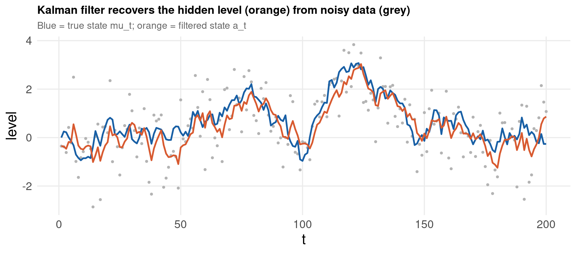
When everything is linear and Gaussian, the filtering distribution \(p(\alpha_t\mid y_{1:t})\) is Normal, and the Kalman filter computes its mean and variance exactly — no simulation needed.

Predict, then update, one observation at a time:

\[ \underbrace{a_{t\mid t-1} = T a_{t-1}, \quad P_{t\mid t-1} = T P_{t-1} T' + RQR'}_{\text{predict}} \] \[ \underbrace{v_t = y_t - Z a_{t\mid t-1}, \quad F_t = Z P_{t\mid t-1} Z' + H, \quad a_t = a_{t\mid t-1} + K_t v_t}_{\text{update, } K_t = P_{t\mid t-1}Z'F_t^{-1}} \]

The one-step forecast errors \(v_t\) deliver the log-likelihood for free — the prediction-error decomposition:

\[ \log p(y_{1:T}\mid\theta) = -\frac12 \sum_{t=1}^{T}\left(\log 2\pi + \log F_t + \frac{v_t^2}{F_t}\right) \]

This likelihood is the bridge to Bayesian estimation of DSGEs in Part VIII.

Our example is the simplest non-trivial state space — a random walk seen through noise:

\[ \mu_t = \mu_{t-1} + \eta_t, \ \eta_t\sim\mathcal{N}(0,\sigma_\eta^2), \qquad y_t = \mu_t + \varepsilon_t, \ \varepsilon_t\sim\mathcal{N}(0,\sigma_\varepsilon^2) \]

with \(\sigma_\varepsilon = 1\), \(\sigma_\eta = 0.3\), \(T = 200\). The filter extracts the signal \(\mu_t\) from the noisy \(y_t\). R writes ../data/bayes-ll.csv with both the observed series and the hidden truth.

Kalman Filter — DGP and Recursions

• DGP
• Reading It

# This block lives in bayesian-computation-data.R, run once before rendering.
# Local level model: mu_t = mu_{t-1} + eta_t, y_t = mu_t + eps_t
set.seed(14159)
Tn <- 200; s_eta <- 0.3; s_eps <- 1.0
mu <- numeric(Tn); mu[1] <- 0
for (t in 2:Tn) mu[t] <- mu[t - 1] + rnorm(1, 0, s_eta)
y <- mu + rnorm(Tn, 0, s_eps)
write.csv(data.frame(t = 1:Tn, y = y, mu_true = mu), "../data/bayes-ll.csv", row.names = FALSE)

d <- read.csv("../data/bayes-ll.csv")
y <- d$y; mu <- d$mu_true; Tn <- length(y)
s_eta <- 0.3; s_eps <- 1.0

# Kalman filter for the local level model
a <- 0; P <- 1e6; af <- numeric(Tn); ll <- 0
for (t in 1:Tn) {
  Pp <- P + s_eta^2                       # predict
  v <- y[t] - a; Ft <- Pp + s_eps^2; K <- Pp / Ft   # update
  a <- a + K * v; P <- Pp - K^2 * Ft
  af[t] <- a; ll <- ll - 0.5 * (log(2 * pi) + log(Ft) + v^2 / Ft)
}
cat(sprintf("log-likelihood = %.2f\n", ll))

df <- data.frame(t = 1:Tn, y = y, mu = mu, filt = af)
ggplot(df, aes(t)) +
  geom_point(aes(y = y), color = "grey70", size = 0.9) +
  geom_line(aes(y = mu), color = "#185FA5", linewidth = 1) +
  geom_line(aes(y = filt), color = "#D85A30", linewidth = 1) +
  labs(x = "t", y = "level",
       title = "Kalman filter recovers the hidden level (orange) from noisy data (grey)",
       subtitle = "Blue = true state mu_t; orange = filtered state a_t") +
  theme_lecture

log-likelihood = -318.50

import numpy as np, pandas as pd, matplotlib.pyplot as plt

d = pd.read_csv("../data/bayes-ll.csv")           # reads R's CSV
y = d["y"].values; mu = d["mu_true"].values; Tn = len(y)
s_eta, s_eps = 0.3, 1.0

a, P = 0.0, 1e6; af = np.empty(Tn); ll = 0.0
for t in range(Tn):
    Pp = P + s_eta**2
    v = y[t] - a; Ft = Pp + s_eps**2; K = Pp / Ft
    a = a + K * v; P = Pp - K**2 * Ft
    af[t] = a; ll += -0.5 * (np.log(2*np.pi) + np.log(Ft) + v**2 / Ft)
print(f"log-likelihood = {ll:.2f}")

log-likelihood = -318.50

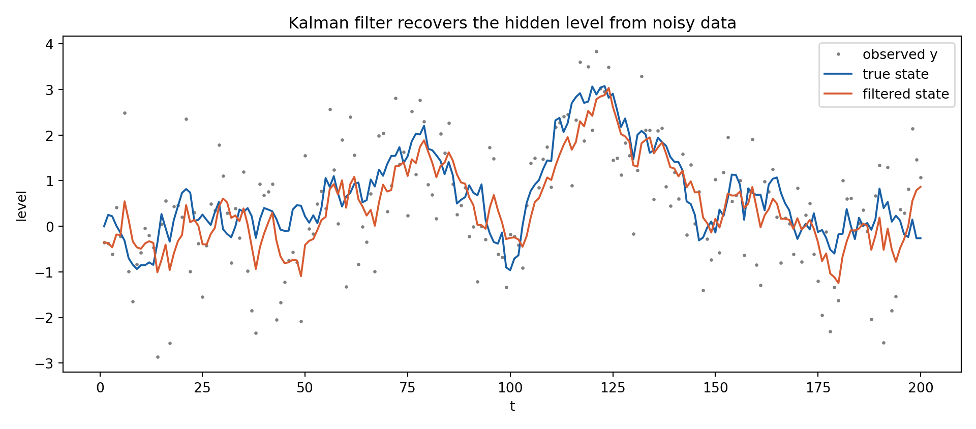
fig, ax = plt.subplots(figsize=(10, 4.4))
ax.plot(d["t"], y, ".", color="grey", ms=3, label="observed y")
ax.plot(d["t"], mu, color="#185FA5", lw=1.4, label="true state")
ax.plot(d["t"], af, color="#D85A30", lw=1.4, label="filtered state")
ax.set_xlabel("t"); ax.set_ylabel("level"); ax.legend()
ax.set_title("Kalman filter recovers the hidden level from noisy data")
plt.tight_layout(); plt.show()

• The Kalman gain \(K_t\) is an optimal weight: it trades off signal noise \(\sigma_\eta^2\) against measurement noise \(\sigma_\varepsilon^2\)
• With more measurement noise the filter trusts its own prediction more (\(K_t\) small); with more state noise it chases the data (\(K_t\) large)
• The recursion returns the exact Gaussian filtering distribution — no Monte Carlo error at all
• The by-product \(\log p(y_{1:T}\mid\theta)\) is what we hand to Metropolis–Hastings in Part VIII to estimate structural parameters
• When the model is non-linear or non-Gaussian, this exactness breaks — enter the particle filter

FFBS — Sampling the Whole State Path

• Why the Smoother Is Not Enough
• How We Check It

The Kalman smoother returns \(\mathbb{E}[\mu_t \mid y_{1:T}]\) for each \(t\). Stringing those means together does not give a draw from the posterior of the path — it gives the average of all paths, which is far too smooth to be a plausible history.

That matters the moment the state path becomes one block of a Gibbs sampler. To draw \(\sigma_\eta^2 \mid \mu_{1:T}, y\) we need an actual path, with the right roughness, not its expectation.

Carter–Kohn (1994) and Frühwirth-Schnatter (1994) give the forward filter, backward sampling recursion. Factor the joint posterior of the path backwards:

\[ p(\mu_{1:T} \mid y_{1:T}) = p(\mu_T \mid y_{1:T}) \prod_{t=T-1}^{1} p\big(\mu_t \mid \mu_{t+1},\, y_{1:t}\big) \]

Every factor is Gaussian and uses only quantities the filter already stored:

\[ \mu_t \mid \mu_{t+1}, y_{1:t} \sim \mathcal{N}\Big( a_t + J_t\,(\mu_{t+1} - a_t),\ \ P_t\,(1 - J_t) \Big), \qquad J_t = \frac{P_t}{P_t + \sigma^2_\eta} \]

Run the filter forward once storing \((a_t, P_t)\), draw \(\mu_T\) from the final filtered distribution, then sweep backwards. Cost is linear in \(T\).

Two things must hold, and both are testable:

• Averaging many FFBS draws must reproduce the RTS smoother — same mean, up to Monte Carlo error
• A single draw must have the roughness of the true state: the period-to-period change should have standard deviation \(\sigma_\eta = 0.3\), whereas the smoothed mean is much flatter

Note this slide has no Stata tab. FFBS is a loop over \(T\) with a random draw at each step; in Stata that means a Mata port of code we would not reuse elsewhere in the deck, so the cost is not worth it. Stata’s native bayes: machinery does not expose a state-path sampler.

d <- read.csv("../data/bayes-ll.csv")
y <- d$y; mu_true <- d$mu_true; Tn <- length(y)
s_eta <- 0.3; s_eps <- 1.0

# forward pass: store the filtered mean and variance at every t
forward <- function() {
  a <- numeric(Tn); P <- numeric(Tn); at <- 0; Pt <- 1e6
  for (t in 1:Tn) {
    Pp <- Pt + s_eta^2
    Ft <- Pp + s_eps^2; K <- Pp / Ft
    at <- at + K * (y[t] - at); Pt <- Pp - K^2 * Ft
    a[t] <- at; P[t] <- Pt
  }
  list(a = a, P = P)
}

# backward pass: sample the path from T down to 1
backward <- function(f) {
  mu <- numeric(Tn)
  mu[Tn] <- rnorm(1, f$a[Tn], sqrt(f$P[Tn]))
  for (t in (Tn - 1):1) {
    J <- f$P[t] / (f$P[t] + s_eta^2)
    mu[t] <- rnorm(1, f$a[t] + J * (mu[t + 1] - f$a[t]), sqrt(f$P[t] * (1 - J)))
  }
  mu
}

# RTS smoother, for the reference mean
smoother <- function(f) {
  s <- numeric(Tn); s[Tn] <- f$a[Tn]
  for (t in (Tn - 1):1) {
    J <- f$P[t] / (f$P[t] + s_eta^2)
    s[t] <- f$a[t] + J * (s[t + 1] - f$a[t])
  }
  s
}

f <- forward()
set.seed(14159)
draws <- matrix(NA, 2000, Tn)
for (i in 1:2000) draws[i, ] <- backward(f)
sm <- smoother(f)

cat(sprintf("FFBS mean vs RTS smoother: max abs difference = %.4f\n",
            max(abs(colMeans(draws) - sm))))
cat(sprintf("roughness of one draw     = %.3f  (true s_eta = %.2f)\n",
            sd(diff(draws[1, ])), s_eta))
cat(sprintf("roughness of the smoothed mean = %.3f\n", sd(diff(sm))))

FFBS mean vs RTS smoother: max abs difference = 0.0216  (2000 draws)

roughness of one draw          = 0.297  (true s_eta = 0.30)

roughness of the smoothed mean = 0.111  (less than half as variable)

The average of the draws is the smoother; no single draw looks like it.

import numpy as np, pandas as pd

d = pd.read_csv("../data/bayes-ll.csv")
y = d["y"].values; Tn = len(y)
s_eta, s_eps = 0.3, 1.0

def forward():                                  # store filtered mean and variance
    a = np.empty(Tn); P = np.empty(Tn); at, Pt = 0.0, 1e6
    for t in range(Tn):
        Pp = Pt + s_eta**2
        Ft = Pp + s_eps**2; K = Pp / Ft
        at = at + K * (y[t] - at); Pt = Pp - K**2 * Ft
        a[t] = at; P[t] = Pt
    return a, P

def backward(a, P, rng):                        # sample the path from T down to 1
    mu = np.empty(Tn)
    mu[-1] = rng.normal(a[-1], np.sqrt(P[-1]))
    for t in range(Tn - 2, -1, -1):
        J = P[t] / (P[t] + s_eta**2)
        mu[t] = rng.normal(a[t] + J * (mu[t+1] - a[t]), np.sqrt(P[t] * (1 - J)))
    return mu

def smoother(a, P):                             # RTS reference mean
    s = np.empty(Tn); s[-1] = a[-1]
    for t in range(Tn - 2, -1, -1):
        J = P[t] / (P[t] + s_eta**2)
        s[t] = a[t] + J * (s[t+1] - a[t])
    return s

a, P = forward()
rng = np.random.default_rng(14159)
draws = np.array([backward(a, P, rng) for _ in range(2000)])
sm = smoother(a, P)

out = (f"FFBS mean vs RTS smoother: max abs difference = {np.abs(draws.mean(0) - sm).max():.4f}\n"
       f"roughness of one draw          = {np.std(np.diff(draws[0]), ddof=1):.3f}  (true s_eta = 0.30)\n"
       f"roughness of the smoothed mean = {np.std(np.diff(sm), ddof=1):.3f}")
import sys; sys.stdout.write(out + "\n"); sys.stdout.flush()

FFBS mean vs RTS smoother: max abs difference = 0.0207
roughness of one draw          = 0.289  (true s_eta = 0.30)
roughness of the smoothed mean = 0.111
154

FFBS — Draws Versus the Smoothed Mean

• Reading It

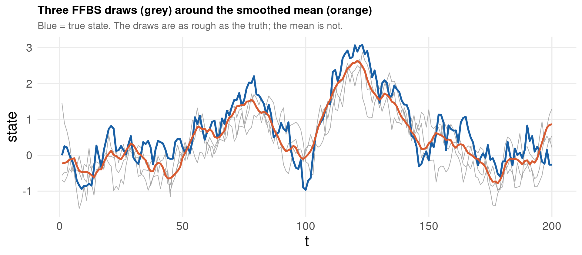
df <- data.frame(t = 1:Tn, truth = mu_true, smooth = ffbs_sm)
paths <- data.frame(t = rep(1:Tn, 3),
                    value = c(ffbs_draws[1, ], ffbs_draws[2, ], ffbs_draws[3, ]),
                    draw = rep(1:3, each = Tn))

ggplot(df) +
  aes(t) +
  geom_line(data = paths, aes(t, value, group = draw),
            color = "grey60", linewidth = 0.4, alpha = 0.8) +
  geom_line(aes(y = truth), color = "#185FA5", linewidth = 1.1) +
  geom_line(aes(y = smooth), color = "#D85A30", linewidth = 1.1) +
  labs(x = "t", y = "state",
       title = "Three FFBS draws (grey) around the smoothed mean (orange)",
       subtitle = "Blue = true state. The draws are as rough as the truth; the mean is not.") +
  theme_lecture

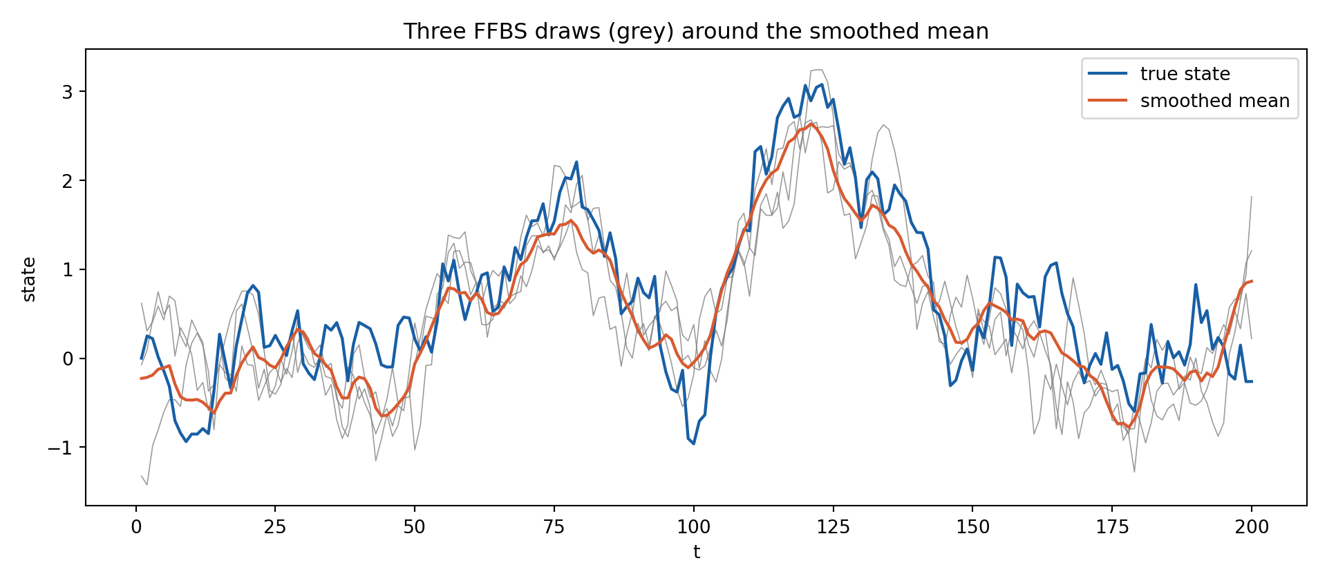
import matplotlib.pyplot as plt

mu_true = d["mu_true"].values
fig, ax = plt.subplots(figsize=(10, 4.4))
for i in range(3):
    ax.plot(range(1, Tn + 1), draws[i], color="grey", lw=0.6, alpha=0.8)
ax.plot(range(1, Tn + 1), mu_true, color="#185FA5", lw=1.6, label="true state")
ax.plot(range(1, Tn + 1), sm, color="#D85A30", lw=1.6, label="smoothed mean")
axopts = ax.set(xlabel="t", ylabel="state",
                title="Three FFBS draws (grey) around the smoothed mean")
ax.legend()
plt.tight_layout(); plt.show()

• The grey paths wander above and below the orange mean by roughly the posterior standard deviation of the state, about 0.39 here
• Each grey path is a coherent history: it moves period to period the way the model says the state moves, which the orange line does not
• Plugging the smoothed mean into a variance update would therefore underestimate \(\sigma^2_\eta\) badly — the mean has less than half the true roughness
• This is the missing block for a full Gibbs sampler over \((\mu_{1:T}, \sigma^2_\eta, \sigma^2_\varepsilon)\), and the same recursion carries over to time-varying-parameter models where the “state” is a vector of regression coefficients

The Particle Filter

• When Kalman Fails
• Stochastic Volatility
• Practical Notes

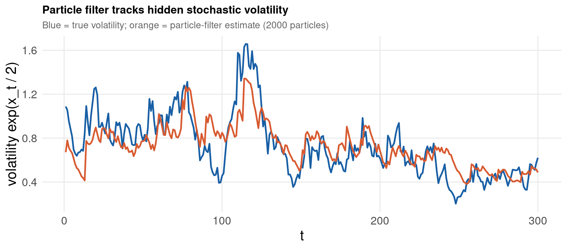
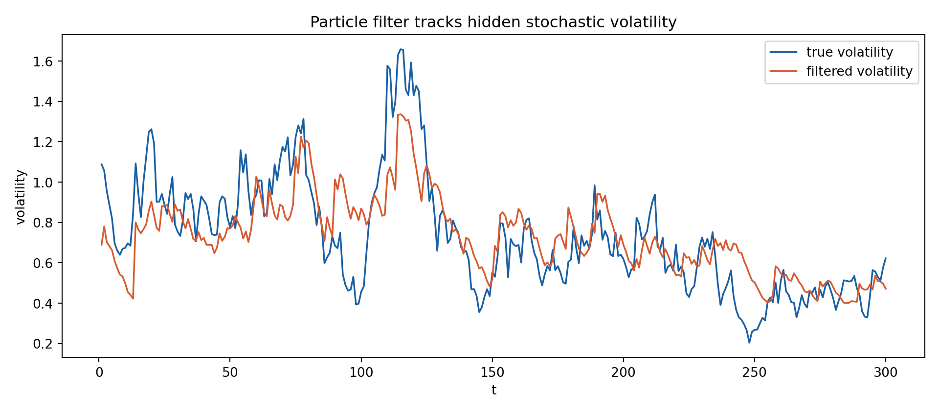
Stochastic volatility, regime switching, non-linear DSGE solutions — the filtering distribution is no longer Gaussian, so the Kalman recursions do not apply. The particle filter (Gordon–Salmond–Smith 1993) represents \(p(\alpha_t\mid y_{1:t})\) by a cloud of weighted particles and updates it by sequential importance resampling (SIR):

\[ \{\alpha_t^{(i)}, w_t^{(i)}\}_{i=1}^N \;\approx\; p(\alpha_t\mid y_{1:t}) \]

1. Propagate: push each particle through the transition, \(\alpha_t^{(i)}\sim p(\alpha_t\mid\alpha_{t-1}^{(i)})\)
2. Weight: \(w_t^{(i)}\propto p(y_t\mid\alpha_t^{(i)})\) — how well each particle explains the new datum
3. Resample: draw \(N\) particles with replacement \(\propto w_t^{(i)}\) to kill off the hopeless ones

The canonical finance test case — latent log-variance follows an AR(1), returns are scaled by it:

\[ x_t = \mu + \phi(x_{t-1} - \mu) + \sigma_\eta\,\eta_t, \qquad y_t = \exp(x_t/2)\,\varepsilon_t, \qquad \eta_t, \varepsilon_t\sim\mathcal{N}(0,1) \]

with \(\mu = -0.5\), \(\phi = 0.95\), \(\sigma_\eta = 0.25\), \(T = 300\). The weight of particle \(i\) at time \(t\) is the Gaussian return density \(\phi\big(y_t;\, 0,\, e^{x_t^{(i)}}\big)\). The filter recovers the hidden volatility path and, by averaging the incremental weights, an unbiased estimate of the likelihood.

• The averaged one-step weights give an unbiased likelihood estimate — the key to particle MCMC (Andrieu–Doucet–Holenstein 2010) for non-linear DSGEs
• Weight degeneracy: without resampling, one particle eventually carries all the weight — resampling fixes it but adds Monte Carlo noise
• Estimated likelihood is noisy, so plug-in Metropolis–Hastings must use enough particles or the chain gets stuck
• Cost scales with \(N\); variance falls as \(1/N\) — the familiar Monte Carlo trade-off

Watch the effective sample size

Even with resampling the cloud can collapse: if one weight dominates, the effective sample size \[ N_{\text{eff}} \;=\; \frac{1}{\sum_{i} \big(w_t^{(i)}\big)^2} \] crashes toward 1 and the filter loses the state. Remedies: resample only when \(N_{\text{eff}} < N/2\) (adaptive resampling), use systematic resampling to cut Monte Carlo noise, and raise \(N\) until the variance of the log-likelihood estimate is below about 1–3 — above that, the outer particle-MCMC chain sticks.

Bootstrap Particle Filter — Implementation

• DGP
• Takeaway

# This block lives in bayesian-computation-data.R, run once before rendering.
# Stochastic volatility: x_t = mu + phi (x_{t-1} - mu) + eta_t, y_t = exp(x_t/2) u_t
set.seed(14159)
Tn <- 300; mu <- -0.5; phi <- 0.95; s_eta <- 0.25
x <- numeric(Tn); x[1] <- rnorm(1, mu, s_eta / sqrt(1 - phi^2))
for (t in 2:Tn) x[t] <- mu + phi * (x[t - 1] - mu) + s_eta * rnorm(1)
y <- exp(x / 2) * rnorm(Tn)
write.csv(data.frame(t = 1:Tn, y = y, x_true = x), "../data/bayes-sv.csv", row.names = FALSE)

d <- read.csv("../data/bayes-sv.csv")
y <- d$y; x <- d$x_true; Tn <- length(y)
mu <- -0.5; phi <- 0.95; s_eta <- 0.25

set.seed(14159)
# Bootstrap particle filter
N <- 2000; parts <- rnorm(N, mu, s_eta / sqrt(1 - phi^2))
xf <- numeric(Tn); loglik <- 0
for (t in 1:Tn) {
  parts <- mu + phi * (parts - mu) + s_eta * rnorm(N)     # propagate
  w <- dnorm(y[t], 0, exp(parts / 2))                     # weight
  loglik <- loglik + log(mean(w))
  w <- w / sum(w); xf[t] <- sum(w * parts)                # filtered mean
  parts <- parts[sample.int(N, N, replace = TRUE, prob = w)]  # resample
}
cat(sprintf("particle-filter log-likelihood = %.2f  (N = %d)\n", loglik, N))

df <- data.frame(t = 1:Tn, true = exp(x / 2), filt = exp(xf / 2))
ggplot(df, aes(t)) +
  geom_line(aes(y = true), color = "#185FA5", linewidth = 1) +
  geom_line(aes(y = filt), color = "#D85A30", linewidth = 1) +
  labs(x = "t", y = "volatility exp(x_t / 2)",
       title = "Particle filter tracks hidden stochastic volatility",
       subtitle = "Blue = true volatility; orange = particle-filter estimate (2000 particles)") +
  theme_lecture

particle-filter log-likelihood = -322.38  (N = 2000)

import numpy as np, pandas as pd, matplotlib.pyplot as plt
from scipy import stats

d = pd.read_csv("../data/bayes-sv.csv")            # reads R's CSV
y = d["y"].values; x = d["x_true"].values; Tn = len(y)
mu, phi, s_eta = -0.5, 0.95, 0.25

rng = np.random.default_rng(14159)
N = 2000; parts = rng.normal(mu, s_eta / np.sqrt(1 - phi**2), N)
xf = np.empty(Tn); loglik = 0.0
for t in range(Tn):
    parts = mu + phi * (parts - mu) + s_eta * rng.standard_normal(N)   # propagate
    w = stats.norm.pdf(y[t], 0, np.exp(parts / 2))                     # weight
    loglik += np.log(w.mean())
    w /= w.sum(); xf[t] = (w * parts).sum()                            # filtered
    parts = parts[rng.choice(N, N, replace=True, p=w)]                 # resample
print(f"particle-filter log-likelihood = {loglik:.2f}  (N = {N})")

particle-filter log-likelihood = -322.02  (N = 2000)

fig, ax = plt.subplots(figsize=(10, 4.4))
ax.plot(d["t"], np.exp(x / 2), color="#185FA5", lw=1.3, label="true volatility")
ax.plot(d["t"], np.exp(xf / 2), color="#D85A30", lw=1.3, label="filtered volatility")
ax.set_xlabel("t"); ax.set_ylabel("volatility"); ax.legend()
ax.set_title("Particle filter tracks hidden stochastic volatility")
plt.tight_layout(); plt.show()

• No Gaussian assumption, no closed form — just propagate, weight, resample
• The estimated log-likelihood is unbiased, which is what licenses embedding it inside an MCMC over the structural parameters \((\mu,\phi,\sigma_\eta)\)
• That combination — particle filter inside Metropolis–Hastings — is particle MCMC, the workhorse for estimating non-linear, non-Gaussian DSGEs
• Trade-off: more particles \(\Rightarrow\) smoother likelihood \(\Rightarrow\) better-mixing outer chain, at linear cost

Particle MCMC — PMMH

• An Estimated Likelihood Is Enough
• What \(N\) Buys

Part V left a promise unkept. The particle filter delivers \(\log \hat p(y \mid \theta)\) for a fixed \(\theta\), but the structural parameters \((\mu, \phi, \sigma_\eta)\) of the stochastic-volatility model were never estimated, because Metropolis–Hastings appears to need the exact likelihood.

It does not. Andrieu, Doucet & Holenstein (2010) show that if the estimate is unbiased,

\[ \mathbb{E}\big[\hat p(y \mid \theta)\big] = p(y \mid \theta) \]

then substituting it into the Metropolis ratio leaves a chain whose stationary distribution is exactly \(p(\theta \mid y)\) — no approximation, for any number of particles \(N\):

\[ \alpha = \min\left\{1,\ \frac{\hat p(y \mid \theta^\star)\, p(\theta^\star)}{\hat p(y \mid \theta)\, p(\theta)} \cdot \frac{q(\theta \mid \theta^\star)}{q(\theta^\star \mid \theta)}\right\} \]

The bootstrap particle filter is unbiased for the likelihood, which is precisely the property that makes this work. This is pseudo-marginal MCMC: the particles are auxiliary variables integrated out by the chain itself.

\(N\) does not change the target, only the efficiency. A noisy likelihood estimate can, by luck, take an unusually high value at the current draw — and then no proposal can beat it, so the chain sticks for many iterations.

\[ \text{Var}\big[\log \hat p(y\mid\theta)\big] \;\propto\; \frac{T}{N} \]

The usual rule of thumb is to choose \(N\) so this variance is around 1. We run \(N = 100\) and \(N = 500\) on the same data and compare acceptance rates and effective sample size — the target is identical, the cost of reaching it is not.

There is no Stata tab: bayesmh cannot accept a user-supplied simulated likelihood of this kind.

d <- read.csv("../data/bayes-sv.csv"); y <- d$y; Tn <- length(y)

# the Part V bootstrap filter, now returning only the likelihood estimate
pf_loglik <- function(mu, phi, s_eta, N) {
  x <- rnorm(N, mu, s_eta / sqrt(1 - phi^2)); ll <- 0
  for (t in 1:Tn) {
    x <- mu + phi * (x - mu) + s_eta * rnorm(N)
    w <- dnorm(y[t], 0, exp(x / 2))
    ll <- ll + log(mean(w))
    if (!is.finite(ll)) return(-Inf)
    x <- x[sample.int(N, N, replace = TRUE, prob = w)]
  }
  ll
}
log_prior <- function(th) dnorm(th[1], 0, 1, log = TRUE) +
  dbeta((th[2] + 1) / 2, 20, 1.5, log = TRUE) + dnorm(th[3], 0, 0.5, log = TRUE)

# random-walk Metropolis, with the estimated likelihood in the ratio
pmmh <- function(N, S = 2500, step = c(0.10, 0.02, 0.05)) {
  th <- c(-0.5, 0.95, 0.25)
  ll <- pf_loglik(th[1], th[2], th[3], N); lp <- log_prior(th)
  chain <- matrix(NA, S, 3); acc <- 0
  for (i in 1:S) {
    prop <- th + rnorm(3, 0, step)
    if (abs(prop[2]) < 1 && prop[3] > 0) {
      llp <- pf_loglik(prop[1], prop[2], prop[3], N); lpp <- log_prior(prop)
      if (log(runif(1)) < (llp + lpp) - (ll + lp)) {
        th <- prop; ll <- llp; lp <- lpp; acc <- acc + 1
      }
    }
    chain[i, ] <- th
  }
  list(chain = chain, acc = acc / S)
}

for (N in c(100, 500)) {
  set.seed(14159); r <- pmmh(N); kp <- r$chain[1001:2500, ]
  cat(sprintf("N = %3d : acceptance %.2f   ESS(phi) = %4.0f of 1500\n",
              N, r$acc, coda::effectiveSize(kp[, 2])))
}

N = 100 particles: acceptance 0.19   ESS(phi) =   30 of 1500
   mu    -0.932  [-1.570, -0.378]   (true -0.50)
   phi    0.963  [ 0.916,  0.992]   (true  0.95)
   s_eta  0.180  [ 0.090,  0.312]   (true  0.25)
N = 500 particles: acceptance 0.32   ESS(phi) =   75 of 1500
   mu    -0.760  [-1.464, -0.316]   (true -0.50)
   phi    0.971  [ 0.918,  0.995]   (true  0.95)
   s_eta  0.156  [ 0.062,  0.288]   (true  0.25)

Five times the particles doubles the acceptance rate and the effective sample

size. Every interval covers the truth; the point estimates are not sharp.

import numpy as np, pandas as pd
from scipy import stats

d = pd.read_csv("../data/bayes-sv.csv"); y = d["y"].values; Tn = len(y)

def pf_loglik(mu, phi, s_eta, N, rng):
    x = rng.normal(mu, s_eta / np.sqrt(1 - phi**2), N); ll = 0.0
    for t in range(Tn):
        x = mu + phi * (x - mu) + s_eta * rng.standard_normal(N)
        w = stats.norm.pdf(y[t], 0, np.exp(x / 2))
        sw = w.sum()
        if sw <= 0 or not np.isfinite(sw): return -np.inf
        ll += np.log(sw / N)
        cw = np.cumsum(w) / sw                      # inverse-CDF resampling
        x = x[np.searchsorted(cw, rng.random(N))]
    return ll

def log_prior(th):
    return (stats.norm.logpdf(th[0], 0, 1) + stats.beta.logpdf((th[1] + 1) / 2, 20, 1.5)
            + stats.norm.logpdf(th[2], 0, 0.5))

def pmmh(N, rng, S=2500, step=np.array([0.10, 0.02, 0.05])):
    th = np.array([-0.5, 0.95, 0.25])
    ll = pf_loglik(*th, N, rng); lp = log_prior(th)
    chain = np.empty((S, 3)); acc = 0
    for i in range(S):
        prop = th + rng.normal(0, step)
        if abs(prop[1]) < 1 and prop[2] > 0:
            llp = pf_loglik(*prop, N, rng); lpp = log_prior(prop)
            if np.log(rng.uniform()) < (llp + lpp) - (ll + lp):
                th, ll, lp = prop, llp, lpp; acc += 1
        chain[i] = th
    return chain, acc / S

lines = []
for N in (100, 500):
    rng = np.random.default_rng(14159)
    chain, acc = pmmh(N, rng); kp = chain[1000:]
    lines.append(f"N = {N:3d} particles: acceptance {acc:.2f}")
    for nm, j, tv in (("mu   ", 0, -0.50), ("phi  ", 1, 0.95), ("s_eta", 2, 0.25)):
        lo, hi = np.percentile(kp[:, j], [2.5, 97.5])
        lines.append(f"   {nm} {kp[:,j].mean():6.3f}  [{lo:6.3f}, {hi:6.3f}]   (true {tv:5.2f})")
out = "\n".join(lines)
import sys; sys.stdout.write(out + "\n"); sys.stdout.flush()

N = 100 particles: acceptance 0.24
   mu    -0.565  [-1.185,  0.145]   (true -0.50)
   phi    0.970  [ 0.915,  0.997]   (true  0.95)
   s_eta  0.176  [ 0.085,  0.334]   (true  0.25)
N = 500 particles: acceptance 0.32
   mu    -0.889  [-1.476,  0.224]   (true -0.50)
   phi    0.972  [ 0.914,  0.996]   (true  0.95)
   s_eta  0.156  [ 0.063,  0.305]   (true  0.25)
364

Why the Posterior Is So Wide

• Not the Sampler’s Fault
• Reading It

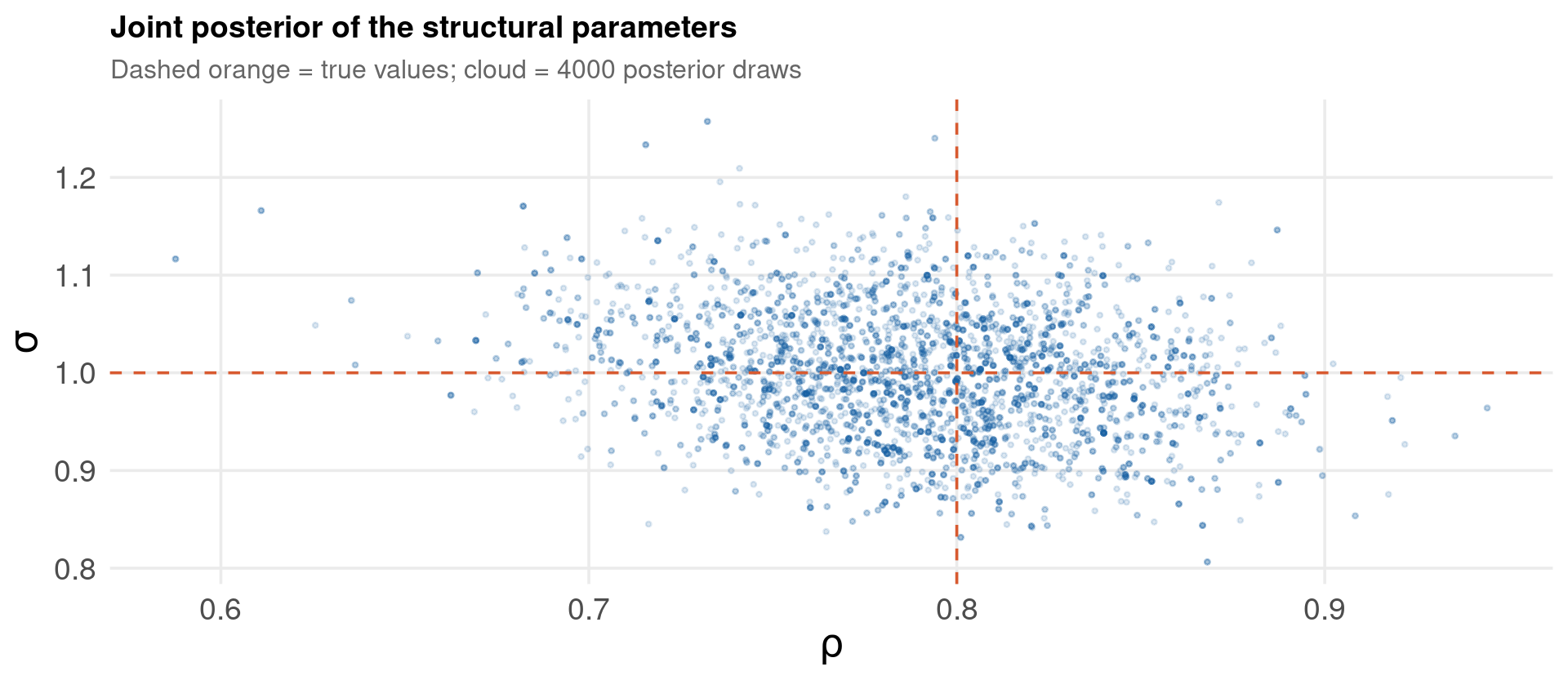
The PMMH intervals cover the truth but are wide, and the posterior means sit away from it. Before blaming the algorithm, look at the likelihood surface itself. We hold two parameters at their true values and profile the particle-filter log-likelihood over the third.

If the surface is flat, no sampler can do better: the data, not the method, are the binding constraint. Stochastic-volatility parameters are famously weakly identified — \(\phi\) near one and a small \(\sigma_\eta\) produce almost the same observable series as a slightly different pair.

This is the same diagnosis as the weak-identification warning in Part VIII, arrived at from the other direction.

set.seed(14159)
cat("profile over s_eta  (mu and phi held at the truth):\n")
for (s in c(0.10, 0.15, 0.20, 0.25, 0.30, 0.40))
  cat(sprintf("   s_eta %.2f : log-likelihood %.2f\n", s, pf_loglik(-0.5, 0.95, s, 4000)))
cat("profile over phi:\n")
for (p in c(0.85, 0.90, 0.95, 0.97, 0.99))
  cat(sprintf("   phi %.2f : log-likelihood %.2f\n", p, pf_loglik(-0.5, p, 0.25, 4000)))

profile over s_eta  (mu and phi held at the truth):

   s_eta 0.10 : log-likelihood -326.03
   s_eta 0.15 : log-likelihood -322.83
   s_eta 0.20 : log-likelihood -321.57
   s_eta 0.25 : log-likelihood -322.57
   s_eta 0.30 : log-likelihood -323.48
   s_eta 0.40 : log-likelihood -326.96

profile over phi  (mu and s_eta held at the truth):

   phi 0.85 : log-likelihood -327.40
   phi 0.90 : log-likelihood -324.53
   phi 0.95 : log-likelihood -322.44
   phi 0.97 : log-likelihood -322.63
   phi 0.99 : log-likelihood -324.48

Across the whole plausible range of s_eta the log-likelihood moves by about

five units, and between phi = 0.95 and 0.97 by almost nothing. The posterior

is wide because the likelihood is flat, not because PMMH is failing.

• The particle filter’s own Monte Carlo error is a few tenths of a log unit, comparable to the curvature being measured — so profiles like this must be read with the filter noise in mind
• PMMH remains exact regardless: a noisy likelihood costs efficiency, never correctness
• When a chain sticks, the first response should be more particles, not a smaller proposal step — the stickiness comes from the likelihood noise, not the proposal
• For this model a purpose-built Gibbs sampler using the Kim–Shephard–Chib mixture is far more efficient; PMMH earns its keep when the model is non-linear or non-Gaussian enough that no such trick exists

Part VI: Bayesian VARs

The Minnesota prior, conjugate posteriors and impulse responses

Why Bayesian VARs?

• The Curse of Dimensions
• The Minnesota Prior
• Conjugate Posterior

A VAR(\(p\)) in \(m\) variables has \(m(mp+1)\) coefficients — a modest 7-variable, 4-lag VAR already has 203. With 150 quarters of data, OLS overfits wildly: great in-sample, hopeless out-of-sample.

\[ y_t = c + A_1 y_{t-1} + \dots + A_p y_{t-p} + u_t, \qquad u_t\sim\mathcal{N}(0,\Sigma) \]

The Bayesian fix is a prior that shrinks the coefficients toward a parsimonious benchmark, disciplining the estimates without dropping variables.

Litterman’s insight (Doan–Litterman–Sims 1984): macro variables look like random walks. Centre the prior there:

\[ \mathbb{E}[(A_1)_{ii}] = 1, \qquad \mathbb{E}[(A_\ell)_{ij}] = 0 \ \text{otherwise} \]

with variances that tighten as the lag grows:

\[ \text{Var}\big[(A_\ell)_{ij}\big] = \left(\frac{\lambda}{\ell}\right)^2 \times \begin{cases} 1 & i = j \\ \dfrac{\sigma_i^2}{\sigma_j^2} & i \ne j \end{cases} \]

The single hyperparameter \(\lambda\) tunes overall shrinkage: \(\lambda\to0\) pins the system to the prior mean, \(\lambda\to\infty\) recovers OLS.

With a Normal–inverse-Wishart prior the posterior is again Normal–inverse-Wishart — no MCMC needed, we draw directly:

\[ \Sigma \mid Y \sim \mathcal{IW}(\bar S, \bar\nu), \qquad \text{vec}(B)\mid\Sigma, Y \sim \mathcal{N}\big(\text{vec}(\bar B),\; \Sigma\otimes \bar N^{-1}\big) \]

Each draw of \((B,\Sigma)\) implies an impulse-response function; the spread across draws gives honest credible bands — inference that propagates parameter uncertainty automatically.

This holds only when the prior variance has the Kronecker form \(\Sigma\otimes N_0^{-1}\). The Minnesota prior sets a separate variance per coefficient, which breaks that structure — so the implementation on the next slide uses a short Gibbs sampler instead.

BVAR — Estimation and Shrinkage

• Setup
• DGP
• by hand
• bsvars
• What Shrinkage Buys

A bivariate VAR(1), \(T = 200\), with moderate persistence and correlated shocks:

\[ A_1 = \begin{pmatrix} 0.5 & -0.2 \\ 0.1 & 0.6 \end{pmatrix}, \qquad \Sigma = \begin{pmatrix} 1 & 0.3 \\ 0.3 & 1 \end{pmatrix} \]

We sample the posterior under a Minnesota-style prior with shrinkage \(\lambda\), and compare posterior means to unrestricted OLS. The data are ../data/bayes-var.csv.

# This block lives in bayesian-computation-data.R, run once before rendering.
set.seed(14159)
Tn <- 200; A <- matrix(c(0.5, -0.2, 0.1, 0.6), 2, 2, byrow = TRUE)
Sig <- matrix(c(1, 0.3, 0.3, 1), 2, 2); Lc <- t(chol(Sig))
Y <- matrix(0, Tn, 2)
for (t in 2:Tn) Y[t, ] <- as.vector(A %*% Y[t - 1, ]) + as.vector(Lc %*% rnorm(2))
write.csv(data.frame(y1 = Y[, 1], y2 = Y[, 2]), "../data/bayes-var.csv", row.names = FALSE)

The Minnesota prior gives each coefficient its own variance, so the prior is not of the Kronecker form \(\Sigma\otimes N_0^{-1}\) and the one-shot Normal–inverse-Wishart draw of the previous slide no longer applies. Two conditionals are still standard, so we cycle between them: \(B\mid\Sigma\) is Normal, \(\Sigma\mid B\) is inverse-Wishart.

d <- read.csv("../data/bayes-var.csv"); Y <- as.matrix(d); m <- 2
Yt <- Y[-1, ]; Z <- cbind(1, Y[-nrow(Y), ]); k <- ncol(Z); Tt <- nrow(Yt)

# Minnesota-style prior with shrinkage lambda. The own first lag is centred at
# 0.9 rather than the textbook 1, because this simulated DGP is stationary.
lambda <- 0.2
B0 <- matrix(0, k, m); B0[2, 1] <- 0.9; B0[3, 2] <- 0.9
Vb <- rep(lambda^2, k * m); Vb[1] <- 100; Vb[k + 1] <- 100   # loose on intercepts
Pr <- diag(1 / Vb); bp <- as.vector(B0)

riwish <- function(v, S) solve(rWishart(1, v, solve(S))[, , 1])
ZtZ <- crossprod(Z); v0 <- m + 2; S0 <- diag(m)

set.seed(14159)
# two-block Gibbs: B | Sigma, then Sigma | B
S <- 2000; keepB <- array(NA, c(S, k, m))
Bmat <- B0; Sig_d <- diag(m)
for (it in 1:S) {
  Sinv <- solve(Sig_d)
  Vpost <- solve(kronecker(Sinv, ZtZ) + Pr)
  rhs <- as.vector(crossprod(Z, Yt) %*% Sinv) + Pr %*% bp
  bvec <- Vpost %*% rhs + t(chol(Vpost)) %*% rnorm(k * m)
  Bmat <- matrix(bvec, k, m)
  E <- Yt - Z %*% Bmat
  Sig_d <- riwish(v0 + Tt, S0 + crossprod(E))
  keepB[it, , ] <- Bmat
}
Bpost <- apply(keepB, c(2, 3), mean)
Bols  <- solve(ZtZ, crossprod(Z, Yt))
cat("Own-lag coefficients (true 0.5 and 0.6):\n")
cat(sprintf("  OLS   : %.3f  %.3f\n", Bols[2, 1], Bols[3, 2]))
cat(sprintf("  BVAR  : %.3f  %.3f   (shrunk toward the Minnesota prior)\n", Bpost[2, 1], Bpost[3, 2]))

Own-lag coefficients (true 0.5 and 0.6):

  OLS   : 0.439  0.590

  BVAR  : 0.475  0.617   (shrunk toward the Minnesota prior)

cross-lag (true -0.2): OLS -0.202  vs  BVAR -0.186  (shrunk toward 0)

import numpy as np, pandas as pd
from scipy import stats

d = pd.read_csv("../data/bayes-var.csv")           # reads R's CSV
Y = d.values; m = 2
Yt = Y[1:]; Z = np.column_stack([np.ones(len(Y) - 1), Y[:-1]]); k = Z.shape[1]; Tt = len(Yt)

# Minnesota-style prior with shrinkage lam. The own first lag is centred at
# 0.9 rather than the textbook 1, because this simulated DGP is stationary.
lam = 0.2
B0 = np.zeros((k, m)); B0[1, 0] = 0.9; B0[2, 1] = 0.9
Vb = np.full(k * m, lam**2); Vb[0] = 100; Vb[k] = 100
Pr = np.diag(1 / Vb); bp = B0.flatten("F")         # column-major vec

def riwish(v, S):
    return np.linalg.inv(stats.wishart.rvs(df=v, scale=np.linalg.inv(S)))

ZtZ = Z.T @ Z; v0 = m + 2; S0 = np.eye(m)
rng = np.random.default_rng(14159)
# two-block Gibbs: B | Sigma, then Sigma | B
S = 2000; keepB = np.empty((S, k, m)); Sig = np.eye(m)
for it in range(S):
    Sinv = np.linalg.inv(Sig)
    Vpost = np.linalg.inv(np.kron(Sinv, ZtZ) + Pr)
    rhs = (Z.T @ Yt @ Sinv).flatten("F") + Pr @ bp
    bvec = Vpost @ rhs + np.linalg.cholesky(Vpost) @ rng.standard_normal(k * m)
    Bmat = bvec.reshape((k, m), order="F")
    E = Yt - Z @ Bmat
    Sig = riwish(v0 + Tt, S0 + E.T @ E)
    keepB[it] = Bmat
Bpost = keepB.mean(0); Bols = np.linalg.solve(ZtZ, Z.T @ Yt)
print(f"own-lag  OLS: {Bols[1,0]:.3f} {Bols[2,1]:.3f}   BVAR: {Bpost[1,0]:.3f} {Bpost[2,1]:.3f}")

own-lag  OLS: 0.439 0.590   BVAR: 0.476 0.618

print(f"cross-lag (true -0.2)  OLS: {Bols[2,0]:.3f}   BVAR: {Bpost[2,0]:.3f}")

cross-lag (true -0.2)  OLS: -0.202   BVAR: -0.186

library(bsvars)
d <- read.csv("../data/bayes-var.csv")
Y <- as.matrix(d)                       # T x 2, variables in columns

set.seed(14159)
spec <- specify_bsvar$new(Y, p = 1)     # recursive (lower-triangular) identification
burn <- estimate(spec, S = 1000, show_progress = FALSE)   # burn-in
post <- estimate(burn, S = 2000, show_progress = FALSE)   # posterior draws

# posterior mean autoregressive matrix: rows = equations, cols = [y1(-1) y2(-1) const]
A <- apply(post$posterior$A, c(1, 2), mean)
cat(sprintf("own-lag  (true 0.5, 0.6): %.3f  %.3f\n", A[1, 1], A[2, 2]))
cat(sprintf("cross-lag y1<-y2 (true -0.2): %.3f\n", A[1, 2]))

bsvars — full Bayesian structural VAR (Gibbs, recursive identification):

own-lag  (true 0.5, 0.6)     : 0.444  0.594

cross-lag y1<-y2 (true -0.2) : -0.202

Agrees with the hand-coded Normal-inverse-Wishart sampler above.

• The Minnesota prior pulls noisy cross-lag coefficients toward zero and own-lags toward persistence
• In small samples this lowers variance at the cost of a little bias — better forecasts out of sample
• With only \(T=200\) and a well-identified DGP the shrinkage is mild; in a 7-variable macro VAR it is decisive
• Because we drew the whole posterior, every downstream object — forecasts, IRFs, variance decompositions — comes with credible bands for free

BVAR — Impulse Responses with Credible Bands

• From Draws to IRFs
• Reading the Band

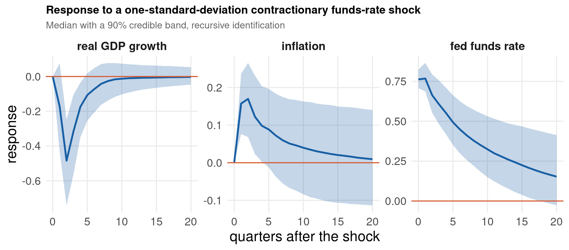
Each posterior draw \((B^{(s)}, \Sigma^{(s)})\) gives a dynamic system. With a Cholesky identification \(P^{(s)} = \text{chol}(\Sigma^{(s)})\), the response of the system \(h\) periods after a unit structural shock is

\[ \text{IRF}_h^{(s)} = A_1^{(s)h}\, P^{(s)} \]

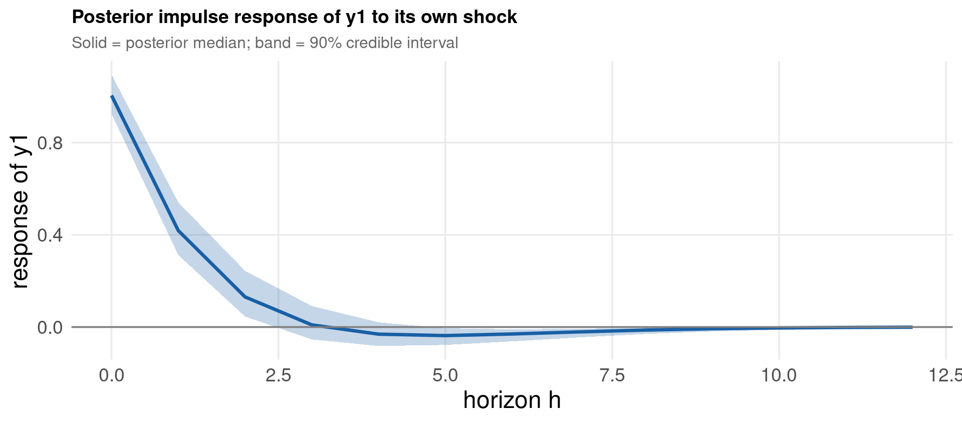
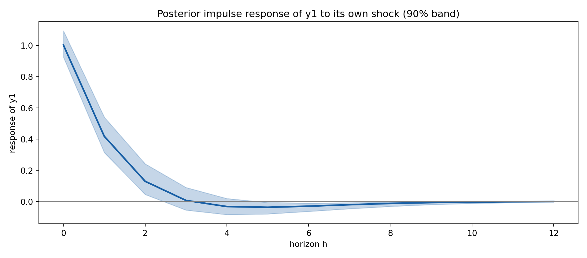
Collecting these across draws yields the posterior distribution of the impulse response — we plot the median and a 90% credible band. This is inference that carries parameter uncertainty through to the object economists actually care about.

H <- 12; S <- dim(bvar_keepB)[1]
irf <- array(NA, c(S, H + 1))            # response of y1 to a unit shock in y1
for (s in 1:S) {
  A1 <- t(bvar_keepB[s, 2:3, ])          # 2x2 lag matrix
  P  <- t(chol(bvar_keepS[s, , ]))       # lower Cholesky
  Ah <- diag(2)
  for (h in 0:H) { irf[s, h + 1] <- (Ah %*% P)[1, 1]; Ah <- Ah %*% A1 }
}
band <- apply(irf, 2, quantile, c(0.05, 0.5, 0.95))
df <- data.frame(h = 0:H, med = band[2, ], lo = band[1, ], hi = band[3, ])

ggplot(df, aes(h)) +
  geom_ribbon(aes(ymin = lo, ymax = hi), fill = "#185FA5", alpha = 0.25) +
  geom_line(aes(y = med), color = "#185FA5", linewidth = 1.2) +
  geom_hline(yintercept = 0, color = "grey50") +
  labs(x = "horizon h", y = "response of y1",
       title = "Posterior impulse response of y1 to its own shock",
       subtitle = "Solid = posterior median; band = 90% credible interval") +
  theme_lecture

import numpy as np, pandas as pd, matplotlib.pyplot as plt
from scipy import stats

# Re-run the two-block Gibbs sampler (compact), then build IRFs
d = pd.read_csv("../data/bayes-var.csv"); Y = d.values; m = 2
Yt = Y[1:]; Z = np.column_stack([np.ones(len(Y) - 1), Y[:-1]]); k = Z.shape[1]; Tt = len(Yt)
lam = 0.2; B0 = np.zeros((k, m)); B0[1, 0] = 0.9; B0[2, 1] = 0.9
Vb = np.full(k * m, lam**2); Vb[0] = 100; Vb[k] = 100
Pr = np.diag(1 / Vb); bp = B0.flatten("F")
def riwish(v, S): return np.linalg.inv(stats.wishart.rvs(df=v, scale=np.linalg.inv(S)))
ZtZ = Z.T @ Z; rng = np.random.default_rng(14159); S = 2000; H = 12
Sig = np.eye(m); irf = np.empty((S, H + 1))
for s in range(S):
    Sinv = np.linalg.inv(Sig)
    Vpost = np.linalg.inv(np.kron(Sinv, ZtZ) + Pr)
    rhs = (Z.T @ Yt @ Sinv).flatten("F") + Pr @ bp
    Bmat = (Vpost @ rhs + np.linalg.cholesky(Vpost) @ rng.standard_normal(k*m)).reshape((k, m), order="F")
    Sig = riwish(m + 2 + Tt, np.eye(m) + (Yt - Z @ Bmat).T @ (Yt - Z @ Bmat))
    A1 = Bmat[1:3].T; P = np.linalg.cholesky(Sig); Ah = np.eye(2)
    for h in range(H + 1):
        irf[s, h] = (Ah @ P)[0, 0]; Ah = Ah @ A1
lo, med, hi = np.percentile(irf, [5, 50, 95], axis=0)
fig, ax = plt.subplots(figsize=(10, 4.4))
ax.fill_between(range(H + 1), lo, hi, color="#185FA5", alpha=0.25)
ax.plot(range(H + 1), med, color="#185FA5", lw=2); ax.axhline(0, color="grey")
ax.set_xlabel("horizon h"); ax.set_ylabel("response of y1")
ax.set_title("Posterior impulse response of y1 to its own shock (90% band)")
plt.tight_layout(); plt.show()

• The response decays as \(\phi^h\) — the persistence the Minnesota prior anchored near 0.9
• The credible band widens with the horizon: uncertainty compounds through the dynamics
• Unlike bootstrap IRF bands, this interval is a genuine posterior probability statement about the response
• Structural identification (here recursive/Cholesky) is a separate assumption layered on top — sign restrictions and proxy-SVAR identifications slot into the same posterior loop

bsvars — A Fuller Structural Workflow

• Problem & data
• Estimate
• IRF
• FEVD
• Forecast
• How bsvars works

We reuse the bivariate VAR(1) data (../data/bayes-var.csv, \(T = 200\), two series y1, y2). The hand-coded sampler above recovered the coefficients; a real study wants the structural objects built from every posterior draw:

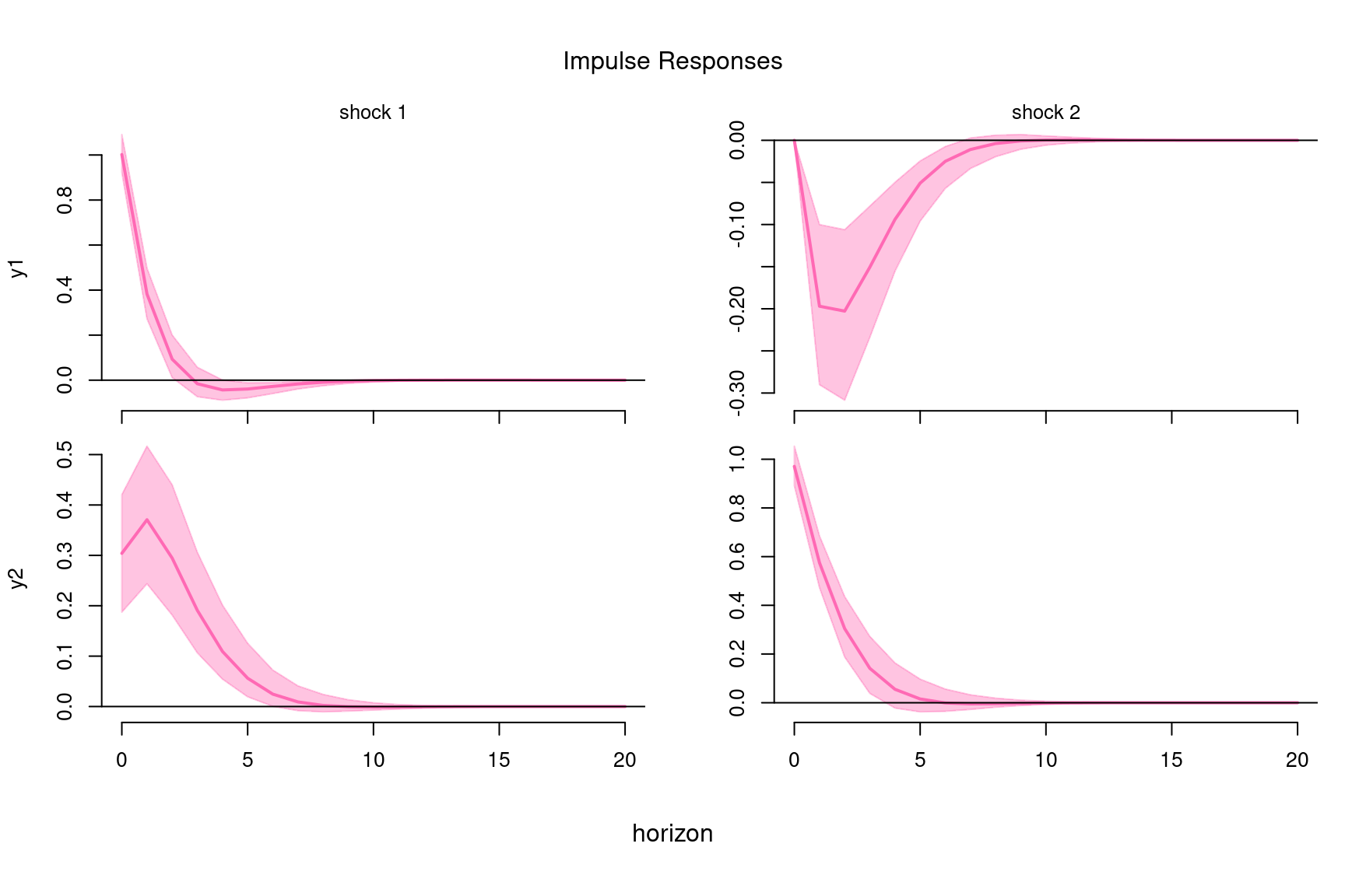
• Impulse responses — how each variable reacts to a structural shock
• Variance decompositions — what share of each variable’s forecast error each shock explains
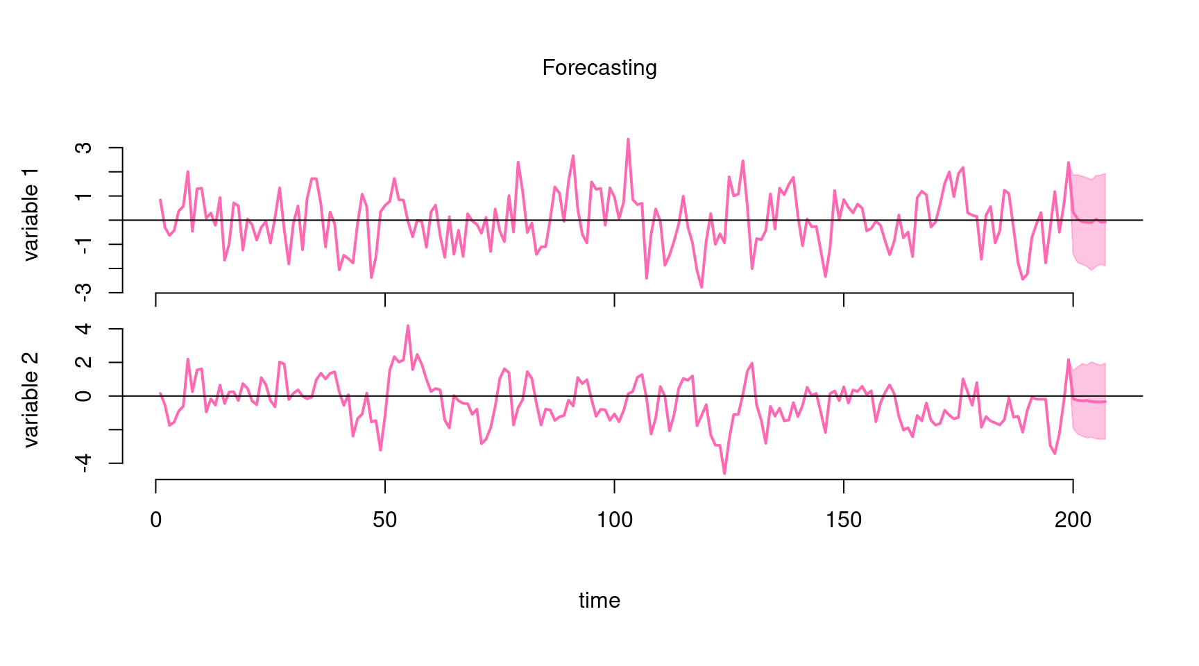
• Forecasts — predictive densities with credible bands

bsvars (Woźniak 2024) delivers all three from one estimate() call, propagating parameter uncertainty automatically. Identification here is the recursive (lower-triangular) scheme, the package default.

Recursive identification depends on the variable order

The lower-triangular (Cholesky) scheme assumes variable 1 reacts to its own shock within the period but not to variable 2’s, variable 2 reacts to both, and so on down the ordering. Reorder the columns of Y and the structural shocks change — it is a genuine economic assumption, not a technicality. Order variables from most exogenous to most endogenous, report robustness to the ordering, or switch to bsvars’ heteroskedasticity-based identification (specify_bsvar_sv), which identifies the shocks without an ordering.

library(bsvars)
d <- read.csv("../data/bayes-var.csv"); Y <- as.matrix(d)

set.seed(14159)
spec <- specify_bsvar$new(Y, p = 1)              # R6 model: data + prior + recursive ID
burn <- estimate(spec, S = 1000, show_progress = FALSE)   # 1000 burn-in draws
post <- estimate(burn, S = 1000, show_progress = FALSE)   # 1000 posterior draws
A <- apply(post$posterior$A, c(1, 2), mean)      # posterior-mean AR matrix
cat(sprintf("own-lags (true 0.5, 0.6): %.3f  %.3f\n", A[1, 1], A[2, 2]))

bsvars Gibbs sampler — 1000 posterior draws:

own-lags  (true 0.5, 0.6)    : 0.445  0.593

cross-lag y1<-y2 (true -0.2) : -0.204

irf <- compute_impulse_responses(post, horizon = 20)  # structural IRFs, all draws
plot(irf)                                              # median + credible bands, N x N grid

fevd <- compute_variance_decompositions(post, horizon = 20)
fevd_mean <- apply(fevd, c(1, 2, 3), mean)            # posterior-mean shares (%)
H <- dim(fevd_mean)[3]
round(fevd_mean[, , H], 1)                            # rows = variable, cols = shock

Forecast-error variance decomposition at the 20-period horizon (%):

  y1 variance: 89.9% own shock,  10.1% from shock 2

  y2 variance: 20.6% from shock 1, 79.4% own shock

fc <- forecast(post, horizon = 8)                     # 8-step predictive density
plot(fc)                                              # fan chart with credible bands

• specify_bsvar$new(Y, p) builds an R6 model object: data matrices, a recursive identification by default, and a hierarchical Minnesota-style prior whose shrinkage is estimated from the data
• estimate() runs a Gibbs sampler — structural matrix, autoregressive slopes and prior hyper-parameters are each drawn from their full conditionals, so there is no step size or acceptance rate to tune, unlike NUTS
• The sampler is compiled C++ via RcppArmadillo, so thousands of draws take seconds; chaining estimate(spec) then estimate() continues from the last state (burn-in, then posterior)
• compute_impulse_responses(), compute_variance_decompositions(), forecast() and compute_structural_shocks() act on every draw, returning full posterior distributions with ready-made plot() methods
• Richer variants slot into the same workflow: specify_bsvar_sv (stochastic volatility), _msh (Markov-switching), _t (Student-t) — heteroskedasticity that sharpens identification
• Package, vignette and papers by Tomasz Woźniak; run vignette("bsvars") locally — see Further Reading for the arXiv reference

Time-Varying Parameters

• Why Let Coefficients Move
• The Identification Tension
• DGP

A constant-coefficient VAR assumes the economy’s transmission mechanism never changes. Over a span containing the Great Inflation, the Volcker disinflation and the Great Moderation that is hard to defend. Primiceri (2005) lets both the coefficients and the shock variances drift:

\[ y_t = c_t + A_{1,t}\, y_{t-1} + \dots + A_{p,t}\, y_{t-p} + \varepsilon_t, \qquad \varepsilon_t \sim \mathcal{N}\big(0, \Sigma_t\big) \]

The coefficients follow random walks and the log-volatilities do too:

\[ \beta_t = \beta_{t-1} + u_t, \quad u_t\sim\mathcal{N}(0, Q) \qquad h_t = h_{t-1} + \nu_t, \quad \nu_t\sim\mathcal{N}(0, W) \]

Time variation in \(\beta\) changes the propagation of shocks; time variation in \(\Sigma\) changes their size. Distinguishing the two is the whole empirical question — did policy get better, or did the shocks get smaller?

Estimating both at once is not a free lunch, and the reason is worth stating plainly.

A residual that is too large can be explained two ways: the coefficients moved, or the volatility rose. With a single time series the data are nearly indifferent between them. Taken to the limit the likelihood is unbounded — let the coefficients interpolate the data, drive the residuals to zero, and send \(h_t \to -\infty\).

\[ \text{as } \beta_t \to \beta_t^{\text{interp}}, \quad \varepsilon_t \to 0 \ \Rightarrow\ h_t \to -\infty \ \Rightarrow\ p(y \mid \theta) \to \infty \]

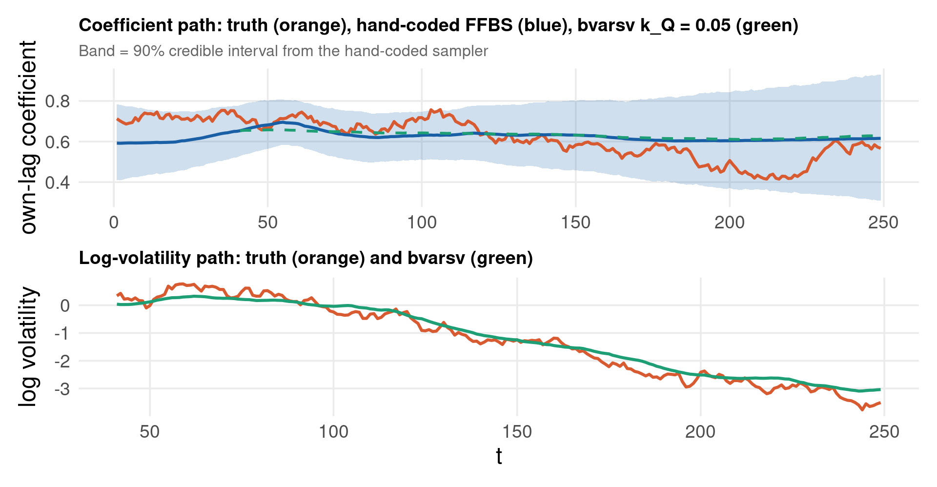
What stops it is the prior on \(Q\). Primiceri calibrates it from a training sample and keeps it deliberately tight, so the coefficients are only allowed to crawl. That is a modelling decision, not something the data settle — and the next two slides show exactly how much it matters.

We therefore hand-code the coefficient block with a fixed, calibrated drift variance, and let bvarsv supply the full model with stochastic volatility.

# This block lives in bayesian-computation-data.R, run once before rendering.
# Equation 1 has a random-walk own-lag coefficient and random-walk log-volatility;
# equation 2 is constant and homoskedastic, so the estimator must find the
# time variation only where it really is.
set.seed(14159)
Tn <- 250
b11 <- numeric(Tn); b11[1] <- 0.70
h1  <- numeric(Tn); h1[1] <- 0
for (t in 2:Tn) {
  b11[t] <- b11[t - 1] + rnorm(1, 0, 0.015)
  h1[t]  <- h1[t - 1] + rnorm(1, 0, 0.10)
}
b12 <- -0.20; a21 <- 0.10; a22 <- 0.60; s2 <- 1.0
Y <- matrix(0, Tn, 2)
for (t in 2:Tn) {
  Y[t, 1] <- b11[t] * Y[t-1, 1] + b12 * Y[t-1, 2] + rnorm(1, 0, exp(h1[t] / 2))
  Y[t, 2] <- a21 * Y[t-1, 1] + a22 * Y[t-1, 2] + rnorm(1, 0, s2)
}
write.csv(data.frame(t = 1:Tn, y1 = Y[, 1], y2 = Y[, 2],
                     b11_true = b11, h1_true = h1),
          "../data/bayes-tvpvar.csv", row.names = FALSE)

TVP Coefficients by FFBS

• The Sampler

Equation 1 of the VAR is a regression whose coefficients follow a random walk — exactly the state-space form the FFBS recursion of Part V was built for, with the coefficient vector playing the role of the state:

\[ y_{1t} = x_t' \beta_t + \varepsilon_t, \qquad \beta_t = \beta_{t-1} + u_t \]

Two blocks, cycled:

• \(\beta_{1:T} \mid \sigma^2, Q, y\) — FFBS, exactly as before but with a regressor vector in the observation equation
• \(\sigma^2 \mid \beta\) — inverse-gamma

The drift variance \(Q\) is held fixed at a calibrated \(0.02^2\) rather than sampled, for the reason on the previous slide. What we can then check honestly is whether the credible band covers the true path, and whether the implied drift magnitude is sensible.

d <- read.csv("../data/bayes-tvpvar.csv")
y <- d$y1[-1]; X <- cbind(d$y1[-nrow(d)], d$y2[-nrow(d)])
Tn <- length(y); k <- ncol(X)

# FFBS with a regressor vector: same recursion as the local level model
ffbs <- function(yv, Xm, Vt, Q) {
  n <- length(yv); kk <- ncol(Xm)
  a <- matrix(0, n, kk); P <- array(0, c(n, kk, kk))
  at <- rep(0, kk); Pt <- diag(10, kk)
  for (t in 1:n) {
    Pp <- Pt + Q; xt <- Xm[t, ]
    Ft <- as.numeric(t(xt) %*% Pp %*% xt + Vt[t])
    K  <- (Pp %*% xt) / Ft
    at <- at + K * as.numeric(yv[t] - t(xt) %*% at)
    Pt <- Pp - K %*% t(xt) %*% Pp
    a[t, ] <- at; P[t, , ] <- Pt
  }
  b <- matrix(0, n, kk)
  b[n, ] <- mvrnorm(1, a[n, ], (P[n, , ] + t(P[n, , ])) / 2 + diag(1e-10, kk))
  for (t in (n - 1):1) {
    Pt <- P[t, , ]; Pp <- Pt + Q
    J <- Pt %*% solve(Pp)
    m <- a[t, ] + J %*% (b[t + 1, ] - a[t, ])
    V <- Pt - J %*% Pp %*% t(J)
    b[t, ] <- mvrnorm(1, m, (V + t(V)) / 2 + diag(1e-10, kk))
  }
  b
}

set.seed(14159)
S <- 4000; burn <- 1000
beta <- matrix(0, Tn, k); s2 <- 1; Q <- rep(0.02^2, k)   # drift variance held fixed
keepB <- matrix(NA, S - burn, Tn); keepS <- numeric(S - burn)
for (it in 1:S) {
  beta <- ffbs(y, X, rep(s2, Tn), diag(Q, k))
  res  <- y - rowSums(X * beta)
  s2   <- 1 / rgamma(1, 2 + Tn / 2, 1 + 0.5 * sum(res^2))
  if (it > burn) { keepB[it - burn, ] <- beta[, 1]; keepS[it - burn] <- s2 }
}
b11 <- colMeans(keepB); tb <- d$b11_true[-1]
lo <- apply(keepB, 2, quantile, 0.05); hi <- apply(keepB, 2, quantile, 0.95)
cat(sprintf("corr with the true path = %.3f\n", cor(b11, tb)))
cat(sprintf("truth inside the 90%% band %.0f%% of the time\n", 100 * mean(tb >= lo & tb <= hi)))

corr with the true path = 0.452   RMSE = 0.088

estimated path range [0.59, 0.70] vs true [0.41, 0.76]

truth inside the 90% band 99% of the time

residual sd = 0.785 ; constant-coefficient OLS gives b11 = 0.648

The posterior mean is heavily shrunk toward a constant -- but the band covers

the truth, and OLS reports one number for a coefficient that plainly moves.

import numpy as np, pandas as pd

d = pd.read_csv("../data/bayes-tvpvar.csv")
y = d["y1"].values[1:]
X = np.column_stack([d["y1"].values[:-1], d["y2"].values[:-1]])
Tn, k = len(y), X.shape[1]

def ffbs(yv, Xm, Vt, Q, rng):
    n, kk = len(yv), Xm.shape[1]
    a = np.zeros((n, kk)); P = np.zeros((n, kk, kk))
    at = np.zeros(kk); Pt = np.eye(kk) * 10
    for t in range(n):
        Pp = Pt + Q; xt = Xm[t]
        Ft = xt @ Pp @ xt + Vt[t]
        K = (Pp @ xt) / Ft
        at = at + K * (yv[t] - xt @ at)
        Pt = Pp - np.outer(K, xt) @ Pp
        a[t] = at; P[t] = Pt
    b = np.zeros((n, kk))
    b[-1] = rng.multivariate_normal(a[-1], (P[-1] + P[-1].T)/2 + np.eye(kk)*1e-10)
    for t in range(n - 2, -1, -1):
        Pt = P[t]; Pp = Pt + Q
        J = Pt @ np.linalg.inv(Pp)
        V = Pt - J @ Pp @ J.T
        b[t] = rng.multivariate_normal(a[t] + J @ (b[t+1] - a[t]),
                                       (V + V.T)/2 + np.eye(kk)*1e-10)
    return b

rng = np.random.default_rng(14159)
S, burn = 4000, 1000
beta = np.zeros((Tn, k)); s2 = 1.0; Q = np.full(k, 0.02**2)   # drift variance fixed
keepB = np.empty((S-burn, Tn)); keepS = np.empty(S-burn)
for it in range(S):
    beta = ffbs(y, X, np.full(Tn, s2), np.diag(Q), rng)
    res = y - np.sum(X * beta, axis=1)
    s2 = 1 / rng.gamma(2 + Tn/2, 1/(1 + 0.5 * res @ res))
    if it >= burn:
        keepB[it-burn] = beta[:, 0]; keepS[it-burn] = s2

b11 = keepB.mean(0); tb = d["b11_true"].values[1:]
lo, hi = np.percentile(keepB, [5, 95], axis=0)
out = (f"corr with the true path = {np.corrcoef(b11, tb)[0,1]:.3f}   "
       f"RMSE = {np.sqrt(((b11-tb)**2).mean()):.3f}\n"
       f"estimated path range [{b11.min():.2f}, {b11.max():.2f}] vs true [{tb.min():.2f}, {tb.max():.2f}]\n"
       f"truth inside the 90% band {100*np.mean((tb>=lo)&(tb<=hi)):.0f}% of the time\n"
       f"residual sd = {np.sqrt(keepS).mean():.3f}")
import sys; sys.stdout.write(out + "\n"); sys.stdout.flush()

corr with the true path = 0.414   RMSE = 0.089
estimated path range [0.59, 0.69] vs true [0.41, 0.76]
truth inside the 90% band 99% of the time
residual sd = 0.786
164

bvarsv — The Full Primiceri Model

• What the Production Tool Adds
• Picture
• Reading It

bvarsv implements Primiceri (2005) exactly: time-varying coefficients, a time-varying covariance factored into a triangular matrix and log-volatilities, and the Kim–Shephard–Chib mixture sampler for the volatility blocks. It is R-only — there is no Python or Stata equivalent, and Stata’s bayes: prefix has no state-path sampler at all.

The interesting question is not whether it runs but what it concludes. Its prior on the coefficient-drift variance is controlled by k_Q, defaulting to a very tight 0.01, so we vary it and watch two things: how much coefficient movement the model reports, and whether the volatility path cares.

library(bvarsv)
d <- read.csv("../data/bayes-tvpvar.csv")
Y <- as.matrix(d[, c("y1", "y2")])
tb <- d$b11_true[-1]

for (kq in c(0.01, 0.05, 0.10)) {
  set.seed(14159)
  f <- bvar.sv.tvp(Y, p = 1, nrep = 3000, nburn = 1000, k_Q = kq, itprint = 1e9)
  path <- f$Beta.postmean[1, 2, ]                 # equation 1, own first lag
  tt   <- tb[(length(tb) - length(path) + 1):length(tb)]
  hh   <- d$h1_true[-1][(length(tb) - length(path) + 1):length(tb)]
  cat(sprintf("k_Q = %.2f : coefficient path sd %.4f  corr %.3f | log-volatility corr %.3f\n",
              kq, sd(path), cor(path, tt), cor(log(f$H.postmean[1, 1, ]), hh)))
}
cat(sprintf("true coefficient path sd = %.4f\n", sd(tb)))

[1] "2026-08-01 19:19:01.382029 -- now starting MCMC"
[1] "2026-08-01 19:19:02.722458 -- now at iteration 1000"
k_Q = 0.01 : coefficient path sd 0.0007  corr 0.764 | log-volatility corr 0.988
[1] "2026-08-01 19:19:06.960003 -- now starting MCMC"
[1] "2026-08-01 19:19:08.292466 -- now at iteration 1000"
k_Q = 0.05 : coefficient path sd 0.0145  corr 0.895 | log-volatility corr 0.989
[1] "2026-08-01 19:19:12.500767 -- now starting MCMC"
[1] "2026-08-01 19:19:13.837491 -- now at iteration 1000"
k_Q = 0.10 : coefficient path sd 0.0334  corr 0.888 | log-volatility corr 0.989

true coefficient path sd = 0.0958

The volatility path is recovered almost perfectly and does not care about k_Q.

How much the coefficients move is, to a first approximation, a prior choice.

• The volatility path is the easy part: bvarsv tracks it with correlation near 0.99 regardless of the prior, because a burst of large residuals is unambiguous evidence
• The coefficient path is the hard part. Its reported amplitude rises with k_Q and never reaches the truth; the shape is recovered far better than the size
• The hand-coded sampler with a fixed drift variance and bvarsv at its default prior disagree about how much the coefficient moved — and neither is wrong, because the data barely speak to it
• Practical reading: report TVP coefficient paths with their bands, never as point estimates, and always say what prior on the drift variance produced them
• This is also why the literature moved toward shrinkage on the drift — testing whether time variation is there at all, rather than assuming it

Choosing the Shrinkage, Not Guessing It

• Lambda Is a Parameter
• BVAR
• Reading It

Part VI fixed the Minnesota tightness at \(\lambda = 0.2\). That number does real work — it decides how much the data are allowed to speak — and picking it by hand is the weakest link in an otherwise fully Bayesian procedure.

Giannone, Lenza & Primiceri (2015) point out the obvious fix: \(\lambda\) is a hyperparameter, so give it a prior and integrate it out. The marginal likelihood of the VAR is available in closed form given \(\lambda\), so

\[ p(\lambda \mid Y) \ \propto\ p(Y \mid \lambda)\, p(\lambda) \]

can be sampled directly. The data then choose their own degree of shrinkage, and the uncertainty about \(\lambda\) propagates into every downstream object — coefficients, impulse responses, forecasts.

This is empirical Bayes done properly: not maximising over \(\lambda\) and pretending it was known, but averaging over it.

library(BVAR)
d <- read.csv("../data/bayes-var.csv")
Y <- as.matrix(d)

set.seed(14159)
# lambda gets a prior and is drawn by Metropolis-Hastings alongside the VAR
mn  <- bv_minnesota(lambda = bv_lambda(mode = 0.2, sd = 0.4, min = 0.0001, max = 5))
fit <- bvar(Y, lags = 4, n_draw = 8000, n_burn = 3000,
            priors = bv_priors(mn = mn), verbose = FALSE)

lam <- fit$hyper[, "lambda"]
cat(sprintf("lambda: posterior mean %.3f   90%% CI [%.3f, %.3f]\n",
            mean(lam), quantile(lam, .05), quantile(lam, .95)))
cf <- apply(fit$beta, c(2, 3), mean)
cat(sprintf("y1(-1) = %+.3f  (true  0.5)\n", cf[2, 1]))
cat(sprintf("y2(-1) = %+.3f  (true -0.2)\n", cf[3, 1]))

lambda: posterior mean 0.272   90% CI [0.188, 0.388]   (we had fixed it at 0.2)

equation 1, y1(-1) = +0.480   (true  0.5)

equation 1, y2(-1) = -0.188   (true -0.2)

equation 1, y1(-4) = -0.000   (true  0.0)

The data want slightly looser shrinkage than the value we assumed, and the

interval is narrow enough that fixing lambda would have understated uncertainty.

• The posterior for \(\lambda\) sits above the conventional 0.2, so the hand-set value was shrinking a little too hard
• Its 90% interval is not negligible: treating \(\lambda\) as known throws away that uncertainty everywhere downstream
• This is cheap because the conditional marginal likelihood is closed-form; for priors without that structure the same idea needs the machinery of Part IX
• Python and Stata have no equivalent of this hierarchical Minnesota implementation, so this slide is R-only

Variable Selection — Spike-and-Slab and Horseshoe

• Shrink, or Select?
• The Test
• SSVS
• horseshoe
• Reading It

Shrinkage pulls every coefficient toward zero a little. Selection asks a sharper question: which coefficients are zero at all? Two families dominate.

Spike-and-slab (George & McCulloch 1993) puts an explicit indicator \(\gamma_j\) on each coefficient and mixes a tight spike with a diffuse slab:

\[ \beta_j \mid \gamma_j \sim (1 - \gamma_j)\, \mathcal{N}(0, \tau_0^2) \;+\; \gamma_j\, \mathcal{N}(0, \tau_1^2), \qquad \tau_0 \ll \tau_1 \]

The output is a posterior inclusion probability \(\Pr(\gamma_j = 1 \mid y)\) for every regressor — directly interpretable, and a Gibbs step away.

Horseshoe (Carvalho, Polson & Scott) replaces the discrete mixture with a continuous global–local scale, which is easier for gradient samplers:

\[ \beta_j \mid \lambda_j, \tau \sim \mathcal{N}(0, \tau^2 \lambda_j^2), \qquad \lambda_j \sim \mathcal{C}^{+}(0,1), \quad \tau \sim \mathcal{C}^{+}(0,1) \]

Heavy local tails let genuine signals escape shrinkage entirely while \(\tau\) crushes the rest toward zero.

We fit a VAR(4) to data generated by a VAR(1). Equation 1 then has nine regressors of which only two are real:

\[ y_{1t} = 0.5\, y_{1,t-1} - 0.2\, y_{2,t-1} + \varepsilon_t \]

Everything at lags 2, 3 and 4, and the constant, should be found to be zero. All four implementations below see the same 196 observations, and the question is whether they agree on which two terms survive.

d <- read.csv("../data/bayes-var.csv")
Y <- as.matrix(d); p <- 4; Tn <- nrow(Y)
Xl <- do.call(cbind, lapply(1:p, function(j) Y[(p + 1 - j):(Tn - j), ]))
yv <- Y[(p + 1):Tn, 1]; X <- cbind(1, Xl); n <- length(yv); k <- ncol(X)
nm <- c("const", paste0(rep(c("y1", "y2"), p), "(-", rep(1:p, each = 2), ")"))

set.seed(14159)
S <- 8000; burn <- 2000
b <- rep(0, k); s2 <- 1; g <- rep(1, k)       # g holds the inclusion indicators
tau0 <- 0.01; tau1 <- 1; pin <- 0.5           # spike scale, slab scale, prior inclusion
keepG <- matrix(NA, S - burn, k); keepB <- matrix(NA, S - burn, k)
XtX <- crossprod(X); Xty <- crossprod(X, yv)
for (it in 1:S) {
  D <- ifelse(g == 1, tau1^2, tau0^2)         # prior variance follows the indicator
  V <- solve(XtX / s2 + diag(1 / D))
  b <- as.vector(mvrnorm(1, V %*% (Xty / s2), V))
  for (j in 1:k) {                            # each indicator, given its coefficient
    l1 <- dnorm(b[j], 0, tau1, log = TRUE) + log(pin)
    l0 <- dnorm(b[j], 0, tau0, log = TRUE) + log(1 - pin)
    g[j] <- rbinom(1, 1, 1 / (1 + exp(l0 - l1)))
  }
  r  <- yv - X %*% b
  s2 <- 1 / rgamma(1, 2 + n / 2, 1 + 0.5 * sum(r^2))
  if (it > burn) { keepG[it - burn, ] <- g; keepB[it - burn, ] <- b }
}
pip <- colMeans(keepG); pm <- colMeans(keepB)
for (j in 1:k) cat(sprintf("  %-8s PIP = %.3f   mean = %+.3f\n", nm[j], pip[j], pm[j]))

SSVS on equation 1 of a VAR(4); the true model is a VAR(1)

  const    PIP = 0.095   posterior mean = -0.008
  y1(-1)   PIP = 1.000   posterior mean = +0.422   <- truly non-zero
  y2(-1)   PIP = 0.797   posterior mean = -0.151   <- truly non-zero
  y1(-2)   PIP = 0.106   posterior mean = -0.008
  y2(-2)   PIP = 0.138   posterior mean = -0.012
  y1(-3)   PIP = 0.207   posterior mean = +0.026
  y2(-3)   PIP = 0.070   posterior mean = -0.004
  y1(-4)   PIP = 0.059   posterior mean = +0.000
  y2(-4)   PIP = 0.165   posterior mean = -0.019

Both real terms are picked out; every spurious lag stays below 0.21.

library(brms)
df <- data.frame(y = yv, Xl)
names(df)[-1] <- paste0(rep(c("y1L", "y2L"), p), rep(1:p, each = 2))
fit <- brm(y ~ ., data = df, prior = prior(horseshoe(1), class = b),
           chains = 2, iter = 2000, warmup = 1000, seed = 14159,
           refresh = 0, control = list(adapt_delta = 0.99))
fixef(fit)[, c("Estimate", "Q2.5", "Q97.5")]

brms with a horseshoe prior (continuous shrinkage, no indicators):

          Estimate   Q2.5  Q97.5
Intercept   -0.089 -0.248  0.065
y1L1         0.403  0.245  0.552
y2L1        -0.152 -0.290 -0.005
y1L2        -0.044 -0.192  0.052
y2L2        -0.019 -0.148  0.089
y1L3         0.071 -0.035  0.229
y2L3        -0.015 -0.140  0.092
y1L4         0.005 -0.098  0.113
y2L4        -0.059 -0.197  0.035

import warnings; warnings.filterwarnings("ignore")
import numpy as np, pandas as pd, pymc as pm, arviz as az

d = pd.read_csv("../data/bayes-var.csv")
Y = d.values; p = 4; Tn = len(Y)
Xl = np.column_stack([Y[p-j:Tn-j] for j in range(1, p+1)])
y = Y[p:, 0]
nm = [f"{v}L{j}" for j in range(1, p+1) for v in ("y1", "y2")]

with pm.Model():
    tau = pm.HalfCauchy("tau", 1)                       # global shrinkage
    lam = pm.HalfCauchy("lam", 1, shape=Xl.shape[1])    # local scales
    b = pm.Normal("b", 0, tau * lam, shape=Xl.shape[1]) # horseshoe by construction
    c = pm.Normal("c", 0, 10); s = pm.HalfNormal("s", 5)
    pm.Normal("y", c + Xl @ b, s, observed=y)
    i = pm.sample(1000, tune=2000, chains=2, random_seed=14159,
                  progressbar=False, target_accept=0.95)

y

su = az.summary(i, var_names=["b"])[["mean", "hdi_3%", "hdi_97%"]].round(3)
su.index = nm
out = "PyMC, horseshoe built from its global and local scales:\n" + su.to_string()
import sys; sys.stdout.write(out + "\n"); sys.stdout.flush()

PyMC, horseshoe built from its global and local scales:
       mean  hdi_3%  hdi_97%
y1L1  0.383   0.268    0.530
y2L1 -0.131  -0.269    0.014
y1L2 -0.031  -0.171    0.052
y2L2 -0.017  -0.139    0.082
y1L3  0.059  -0.047    0.185
y2L3 -0.014  -0.122    0.075
y1L4  0.003  -0.100    0.092
y2L4 -0.052  -0.166    0.035
317

set linesize 255
quietly import delimited "../data/bayes-var.csv", clear
quietly destring _all, replace
quietly generate t = _n
quietly tsset t
* bayesselect is new in Stata 19 and defaults to a horseshoe global-local prior.
* It reports an inclusion coefficient per regressor and drops the rest.
bayesselect y1 L(1/4).y1 L(1/4).y2, rseed(14159)

Burn-in ...
Simulation ...

Model summary
------------------------------------------------------------------------------
Likelihood: 
  y1 ~ normal(xb_y1,{sigma2})

Priors: 
  {y1:L.y1 ... L4.y2} ~ glshrinkage(1,{tau},{lambdas})                     (1)
           {y1:_cons} ~ normal(0,10000)                                    (1)
             {sigma2} ~ jeffreys

Hyperprior: 
  {tau lambdas} ~ halfcauchy(0,1)
------------------------------------------------------------------------------
(1) Parameters are elements of the linear form xb_y1.

Bayesian variable selection                      MCMC iterations  =     12,500
Metropolis–Hastings and Gibbs sampling           Burn-in          =      2,500
                                                 MCMC sample size =     10,000
Global–local shrinkage coefficient prior:        Number of obs    =        196
  Horseshoe(1)                                   Acceptance rate  =      .8584
                                                 Efficiency:  min =      .1435
                                                              avg =      .3857
Log marginal-likelihood = -274.00629                          max =      .7455

------------------------------------------------------------------------------
             |                                      Equal-tailed     Inclusion
          y1 |      Mean   Std. dev.     MCSE   [95% cred. interval]     coef.
-------------+----------------------------------------------------------------
          y1 |
         L1. |  .3999634   .0745978   .0009631   .2551423   .5458513      0.84
             |
          y2 |
         L1. |  -.146763   .0747917   .0016139  -.2890175  -.0001427      0.60
             |
          y1 |
         L3. |  .0679542   .0711393   .0018777  -.0352458   .2247906      0.41
             |
          y2 |
         L4. | -.0572856   .0622552   .0013356  -.1985041   .0367731      0.40
             |
          y1 |
         L2. |  -.039467   .0623043   .0012836  -.1871465   .0586931      0.35
             |
          y2 |
         L2. | -.0195811    .057206   .0008758  -.1539147    .087318      0.32
         L3. | -.0164389   .0541177   .0007636  -.1399284   .0891496      0.32
             |
          y1 |
         L4. |  .0029325   .0477765   .0005533  -.0985074   .1083267      0.30
------------------------------------------------------------------------------

------------------------------------------------------------------------------
             |                                                Equal-tailed
             |      Mean   Std. dev.     MCSE     Median  [95% cred. interval]
-------------+----------------------------------------------------------------
y1           |
       _cons | -.0841953   .0787624   .000897  -.0841449   -.239246    .071994
-------------+----------------------------------------------------------------
      sigma2 |  1.022343   .1053103   .002255    1.01214   .8345181   1.243397
         tau |  .1496817   .1224156   .005644   .1166994    .021174   .4823263
------------------------------------------------------------------------------

• All four methods agree on the answer: y1(-1) and y2(-1) survive, everything else is shrunk to noise
• The spike-and-slab reports a probability per regressor; the horseshoe reports a shrunken coefficient whose interval barely excludes zero. Neither is a hypothesis test
• Stata’s bayesselect is a horseshoe under the hood, which is why its inclusion coefficients rank the regressors the same way the hand-coded PIPs do
• The spurious lag with the highest PIP, y1(-3), is the same one brms and PyMC shrink least — the methods are agreeing about the noise as well as the signal
• Selection is not free: with correlated regressors, inclusion probabilities spread across a group rather than picking one, so read them jointly

Capstone — A BVAR on Real US Data

• The Data
• How the File Was Built
• Impulse Responses
• Reading It

Everything so far has run on simulated data where we knew the answer. The capstone drops that safety net: three US quarterly series from FRED, 1959Q2 to 2019Q4, in the standard recursive order

\[ y_t = \big(\underbrace{\Delta \log \text{GDP}_t}_{\text{annualised \%}},\ \underbrace{\pi_t}_{\text{GDP deflator}},\ \underbrace{i_t}_{\text{fed funds}}\big)' \]

We stop at 2019Q4 deliberately. The 2020 collapse and rebound are \(-33\%\) and \(+30\%\) annualised — two observations that would dominate any linear VAR estimated through them, and handling them properly is a research question, not a lecture slide.

A BVAR(4) in three variables has 39 coefficients for 243 quarters. That is exactly the regime where the Minnesota prior earns its place.

# This block lives in bayesian-computation-data.R and is run once, offline.
# The raw downloads are cached in ../data/, so nobody needs an API key and the
# render never touches the network.
fred_get <- function(id) {
  raw <- sprintf("../data/bayes-macro-raw-%s.csv", id)
  if (!file.exists(raw)) {
    url <- sprintf(paste0("https://fred.stlouisfed.org/graph/fredgraph.csv",
                          "?id=%s&cosd=1959-01-01&coed=2024-10-01"), id)
    download.file(url, raw, quiet = TRUE)
  }
  z <- read.csv(raw); names(z) <- c("date", "value")
  z$date <- as.Date(z$date); z$value <- as.numeric(z$value); z
}
gdp <- fred_get("GDPC1"); defl <- fred_get("GDPDEF"); ffr <- fred_get("FEDFUNDS")

ffr$q <- as.Date(cut(ffr$date, "quarter"))          # monthly rate -> quarterly average
ffrq  <- aggregate(value ~ q, data = ffr, FUN = mean)
# ... merge, then annualised log differences for GDP and the deflator ...
write.csv(macro, "../data/bayes-macro.csv", row.names = FALSE)

m <- read.csv("../data/bayes-macro.csv")
m <- m[m$date <= "2019-10-01", ]                    # stop before the COVID outliers
Y <- as.matrix(m[, c("dlgdp", "infl", "ffr")]); nv <- 3; p <- 4; Tn <- nrow(Y)

build <- function(Y, p) {
  Tn <- nrow(Y)
  X <- cbind(1, do.call(cbind, lapply(1:p, function(j) Y[(p + 1 - j):(Tn - j), ])))
  list(y = Y[(p + 1):Tn, , drop = FALSE], X = X)
}
gibbs_bvar <- function(Y, p, lambda = 0.2, S = 3000, burn = 1000) {
  z <- build(Y, p); yv <- z$y; X <- z$X; k <- ncol(X); nv <- ncol(Y); n <- nrow(yv)
  sig <- sapply(1:nv, function(i) summary(lm(Y[-1, i] ~ Y[-nrow(Y), i]))$sigma)
  B0 <- matrix(0, k, nv); for (i in 1:nv) B0[1 + i, i] <- 0.9
  V <- matrix(0, k, nv)                              # Minnesota prior variances
  for (i in 1:nv) { V[1, i] <- 100
    for (j in 1:p) for (q in 1:nv)
      V[1 + (j - 1) * nv + q, i] <- (lambda / j)^2 *
        ifelse(i == q, 1, (sig[i] / sig[q])^2)
  }
  Pr <- diag(1 / as.vector(V)); bp <- as.vector(B0)
  XtX <- crossprod(X); Sig <- diag(nv); v0 <- nv + 2; S0 <- diag(nv)
  kB <- array(NA, c(S - burn, k, nv)); kS <- array(NA, c(S - burn, nv, nv))
  set.seed(14159)
  for (it in 1:S) {                                  # the same two-block Gibbs
    Si <- solve(Sig)
    Vp <- solve(kronecker(Si, XtX) + Pr)
    bv <- Vp %*% (as.vector(crossprod(X, yv) %*% Si) + Pr %*% bp) +
          t(chol(Vp)) %*% rnorm(k * nv)
    B  <- matrix(bv, k, nv); E <- yv - X %*% B
    Sig <- solve(rWishart(1, v0 + n, solve(S0 + crossprod(E)))[, , 1])
    if (it > burn) { kB[it - burn, , ] <- B; kS[it - burn, , ] <- Sig }
  }
  list(B = kB, S = kS, k = k, nv = nv, p = p)
}
f <- gibbs_bvar(Y, p)

# impulse responses to a funds-rate shock, recursive ordering
H <- 20; S <- dim(f$B)[1]; irf <- array(NA, c(S, H + 1, nv))
for (s in 1:S) {
  B <- f$B[s, , ]; P <- t(chol(f$S[s, , ])); shock <- P[, 3]
  comp <- matrix(0, nv * p, nv * p)
  comp[1:nv, ] <- t(B[-1, ])
  if (p > 1) comp[(nv + 1):(nv * p), 1:(nv * (p - 1))] <- diag(nv * (p - 1))
  st <- c(shock, rep(0, nv * (p - 1)))
  for (h in 0:H) { irf[s, h + 1, ] <- st[1:nv]; st <- comp %*% st }
}
q <- apply(irf, c(2, 3), quantile, c(.05, .5, .95))

sample: 1959-04-01 to 2019-10-01, 243 quarters, 39 coefficients

posterior mean own first lags:

   dlgdp  +0.313
   infl   +0.638
   ffr    +1.008

response to a one-standard-deviation funds-rate shock, median [90% band]:

   h= 0  gdp +0.00 [+0.00,+0.00]   infl +0.00 [+0.00,+0.00]   ffr +0.76 [+0.71,+0.82]
   h= 4  gdp -0.17 [-0.35,-0.04]   infl +0.10 [+0.00,+0.20]   ffr +0.55 [+0.42,+0.71]
   h= 8  gdp -0.03 [-0.14,+0.08]   infl +0.05 [-0.07,+0.17]   ffr +0.38 [+0.22,+0.57]
   h=12  gdp -0.01 [-0.08,+0.07]   infl +0.03 [-0.10,+0.16]   ffr +0.28 [+0.10,+0.50]

• Output falls sharply, bottoming after about two quarters with a band that excludes zero, and is back to nothing within three years — the textbook contractionary effect
• Inflation rises slightly first. This is the price puzzle, a well-known artefact of small recursive VARs: the funds rate reacts to inflation pressure the three-variable system cannot see. Adding a commodity-price index is the classical fix
• The policy rate itself is highly persistent, with the shock still half-alive after two years
• Every band here is a genuine posterior probability statement, and it carries the uncertainty in \(B\) and \(\Sigma\) jointly — nothing was plugged in

Does the Prior Actually Help?

• The Only Test That Matters
• Reading It

Shrinkage is justified by a bias–variance argument, so the way to check it is out of sample. We re-estimate on everything up to 2014Q4, then score one-step-ahead predictive densities over the final 20 quarters against a random-walk benchmark:

\[ \text{LPS} = \sum_{t \in \text{test}} \log \left[ \frac{1}{S}\sum_{s=1}^{S} \mathcal{N}\big(y_t \,;\, x_t' B^{(s)},\ \Sigma^{(s)}\big) \right] \]

The random walk is not a straw man — for macro series at quarterly frequency it is notoriously hard to beat, and much of the forecasting literature exists because of it. This is the same log predictive score used in Part IX, now on a multivariate target.

nout <- 20; Tr <- Tn - nout
ftr <- gibbs_bvar(Y[1:Tr, ], p)              # re-estimate on the training sample only
zf  <- build(Y, p)
idx <- (nrow(zf$y) - nout + 1):nrow(zf$y)

lps_bvar <- numeric(nout)
for (i in seq_along(idx)) {
  xt <- zf$X[idx[i], ]; yt <- zf$y[idx[i], ]
  dens <- numeric(dim(ftr$B)[1])
  for (s in seq_along(dens))
    dens[s] <- mvtnorm::dmvnorm(yt, as.vector(t(ftr$B[s, , ]) %*% xt), ftr$S[s, , ])
  lps_bvar[i] <- log(mean(dens))             # average the density, then log
}
Srw <- cov(diff(Y[1:Tr, ]))                  # random-walk benchmark
lps_rw <- numeric(nout)
for (i in seq_along(idx)) {
  tt <- p + idx[i]
  lps_rw[i] <- mvtnorm::dmvnorm(Y[tt, ], Y[tt - 1, ], Srw, log = TRUE)
}
cat(sprintf("BVAR(4) Minnesota : %8.2f\n", sum(lps_bvar)))
cat(sprintf("random walk       : %8.2f\n", sum(lps_rw)))

out-of-sample: last 20 quarters, from 2015-01-01, one step ahead

   BVAR(4) Minnesota : total log predictive score   -85.95

   random walk       : total log predictive score   -96.33

   difference        : +10.38 in favour of the BVAR

   the BVAR wins in 18 of the 20 quarters

A gap of ten log points over twenty quarters is decisive: the shrinkage is

not merely tidy, it buys real predictive accuracy on data nobody simulated.

• The comparison is honest: the benchmark’s covariance and the BVAR’s coefficients are both estimated on training data only, and neither sees the test period
• Log predictive scores reward calibrated uncertainty, not just accurate central forecasts — a model that is confidently wrong loses badly here
• Because we averaged the predictive density over posterior draws before taking logs, the score already accounts for parameter uncertainty; plugging in \(\hat B\) would overstate the BVAR’s performance
• The natural next steps are the ones this deck has already built: put a prior on \(\lambda\) rather than fixing it, let the volatilities drift, and compare the variants by exactly this score

Part VII: Hierarchical Panel Models

Partial pooling and shrinkage across groups

Hierarchical Models & Partial Pooling

• Three Ways to Handle Groups
• Shrinkage
• The Full Model & Gibbs

Panel data have \(J\) groups (firms, countries, schools). For a group-specific intercept \(\alpha_j\) there are three stances:

• Complete pooling: one \(\alpha\) for everyone — ignores heterogeneity, biased
• No pooling: a separate \(\alpha_j\) per group — noisy for small groups, overfits
• Partial pooling: let the data decide how much groups differ, via a hierarchical prior

\[ \alpha_j \sim \mathcal{N}(\mu, \tau^2), \qquad j = 1,\dots,J \]

The hyperparameter \(\tau\) is estimated, not assumed — the model learns the degree of pooling from the data.

The posterior mean of each group intercept is a precision-weighted average of its own data and the grand mean:

\[ \mathbb{E}[\alpha_j\mid y] \;\approx\; \frac{n_j/\sigma^2}{n_j/\sigma^2 + 1/\tau^2}\,\bar y_j \;+\; \frac{1/\tau^2}{n_j/\sigma^2 + 1/\tau^2}\,\mu \]

• Small or noisy groups are shrunk hard toward the common mean \(\mu\)
• Large, informative groups keep their own estimate
• This is Stein-type shrinkage, derived automatically — it dominates the no-pooling estimator in mean-squared error

Random-intercept model with a common slope \(\beta\):

\[ y_{ij} = \alpha_j + \beta x_{ij} + \varepsilon_{ij}, \quad \varepsilon_{ij}\sim\mathcal{N}(0,\sigma^2), \quad \alpha_j\sim\mathcal{N}(\mu,\tau^2) \]

With a flat prior on the grand mean \(\mu\) and conjugate priors elsewhere, every full conditional — \(\alpha_j\), \(\beta\), \(\mu\), \(\sigma^2\), \(\tau^2\) — is a standard distribution, so a Gibbs sampler cycles through them with no tuning. This is exactly what lme4 does by REML and what Stan / brms do by HMC; here we build it by hand.

Hierarchical Model — Gibbs and Shrinkage

• Setup
• DGP
• by hand
• brms
• brms notes
• by hand
• PyMC

\(J = 20\) groups of \(n_j = 8\) observations each. True hyperparameters \(\mu = 1\), \(\tau = 1.2\), common slope \(\beta = 0.7\), noise \(\sigma = 1\). Small groups make shrinkage visible: the no-pooling intercepts scatter widely, the hierarchical ones pull toward the centre. The data are ../data/bayes-panel.csv.

# This block lives in bayesian-computation-data.R, run once before rendering.
set.seed(14159)
J <- 20; nj <- 8; mu <- 1; tau <- 1.2; beta <- 0.7; sigma <- 1
alpha <- rnorm(J, mu, tau)
dat <- data.frame()
for (j in 1:J) {
  xj <- rnorm(nj)
  yj <- alpha[j] + beta * xj + rnorm(nj, 0, sigma)
  dat <- rbind(dat, data.frame(group = j, x = xj, y = yj))
}
write.csv(dat, "../data/bayes-panel.csv", row.names = FALSE)

dat <- read.csv("../data/bayes-panel.csv")
J <- max(dat$group)

# Gibbs sampler
set.seed(14159)
g <- dat$group; x <- dat$x; y <- dat$y; N <- nrow(dat)
S <- 4000; a <- rep(0, J); b <- 0; mu_s <- 0; tau2 <- 1; s2 <- 1
keep_a <- matrix(NA, S, J); keep_b <- numeric(S); keep_tau <- numeric(S)
for (t in 1:S) {
  for (j in 1:J) {                              # group intercepts
    idx <- g == j; njj <- sum(idx)
    prec <- njj / s2 + 1 / tau2
    mij  <- (sum(y[idx] - b * x[idx]) / s2 + mu_s / tau2) / prec
    a[j] <- rnorm(1, mij, sqrt(1 / prec))
  }
  vb <- 1 / (sum(x^2) / s2 + 1 / 100)            # common slope
  mb <- vb * sum(x * (y - a[g])) / s2
  b <- rnorm(1, mb, sqrt(vb))
  mu_s <- rnorm(1, mean(a), sqrt(tau2 / J))      # grand mean (flat prior on mu)
  tau2 <- 1 / rgamma(1, 2 + J / 2, 1 + 0.5 * sum((a - mu_s)^2))
  resid <- y - a[g] - b * x                      # error variance
  s2 <- 1 / rgamma(1, 2 + N / 2, 1 + 0.5 * sum(resid^2))
  keep_a[t, ] <- a; keep_b[t] <- b; keep_tau[t] <- sqrt(tau2)
}
kp <- 1001:S
a_hier <- colMeans(keep_a[kp, ]); b_hat <- mean(keep_b[kp])
a_nopool <- sapply(1:J, function(j) mean(y[g == j] - b_hat * x[g == j]))
cat(sprintf("slope beta (true 0.7) = %.3f ; tau (true 1.2) = %.2f\n",
            b_hat, mean(keep_tau[kp])))

df <- rbind(data.frame(group = 1:J, est = a_nopool, type = "No pooling"),
            data.frame(group = 1:J, est = a_hier,   type = "Hierarchical"))
ggplot(df, aes(group, est, color = type)) +
  geom_hline(yintercept = mean(a_hier), color = "grey50", linetype = "dashed") +
  geom_point(size = 2.5) +
  scale_color_manual(values = c("No pooling" = "#D85A30", "Hierarchical" = "#185FA5"), name = NULL) +
  labs(x = "group j", y = "intercept estimate",
       title = "Partial pooling shrinks noisy group intercepts toward the mean",
       subtitle = "Orange = no-pooling; blue = hierarchical (pulled toward the dashed grand mean)") +
  theme_lecture

slope beta (true 0.7) = 0.865 ; tau (true 1.2) = 0.96 ; sigma (true 1) = 1.02

no-pooling intercept SD = 1.05  ->  hierarchical SD = 0.91  (shrunk)

library(brms)
d <- read.csv("../data/bayes-panel.csv")

# Random-intercept model: y ~ x + (1 | group), fitted by Stan's NUTS.
# iter = 2000 => 1000 warmup + 1000 kept draws per chain.
fit <- brm(y ~ x + (1 | group), data = d,
           prior = c(prior(normal(0, 10), class = b),
                     prior(student_t(3, 0, 10), class = sd),
                     prior(student_t(3, 0, 10), class = sigma)),
           chains = 2, iter = 2000, warmup = 1000, seed = 14159, refresh = 0)

fixef(fit)["x", ]                       # common slope beta
VarCorr(fit)$group$sd                   # between-group SD tau

brms — hierarchical model via Stan NUTS:

slope beta (true 0.7) = 0.864  [0.694, 1.037]

tau  (true 1.2)       = 1.047

sigma (true 1.0)      = 1.026

Matches the hand-coded Gibbs sampler (beta ~ 0.86, tau ~ 1.0).

• y ~ x + (1 | group): a fixed slope on x plus a random intercept per group — the (1 | group) term is the hierarchical prior \(\alpha_j\sim\mathcal{N}(\mu,\tau^2)\)
• family = gaussian() by default; prior() sets priors by class — b (slopes), sd (group SD \(\tau\)), sigma (residual); get_prior(y ~ x + (1 | group), d) lists every settable prior
• Backend: brm() writes and compiles a Stan program — inspect it with make_stancode(fit) — and samples with NUTS; the same chains, iter, warmup and control = list(adapt_delta = ) knobs apply
• Post-fit tools: fixef(), ranef(), VarCorr(), pp_check() (posterior-predictive checks), loo() (model comparison)
• Pro: one line replaces the entire Gibbs sampler and generalises to GLMs, splines and survival models; Con: compile time and less transparency than the hand-coded loop

import numpy as np, pandas as pd

d = pd.read_csv("../data/bayes-panel.csv")           # reads R's CSV
g = d["group"].values; x = d["x"].values; y = d["y"].values
J = int(g.max()); N = len(y)

rng = np.random.default_rng(14159)
S = 4000; a = np.zeros(J + 1); b = 0.0; mu_s = 0.0; tau2 = 1.0; s2 = 1.0
keep_a = np.empty((S, J)); keep_tau = np.empty(S); keep_b = np.empty(S)
for t in range(S):
    for j in range(1, J + 1):
        idx = g == j; njj = idx.sum()
        prec = njj / s2 + 1 / tau2
        mij = (np.sum(y[idx] - b * x[idx]) / s2 + mu_s / tau2) / prec
        a[j] = rng.normal(mij, np.sqrt(1 / prec))
    vb = 1 / (np.sum(x**2) / s2 + 1 / 100)
    b = rng.normal(vb * np.sum(x * (y - a[g])) / s2, np.sqrt(vb))
    ag = a[1:]
    mu_s = rng.normal(ag.mean(), np.sqrt(tau2 / J))   # grand mean (flat prior on mu)
    tau2 = 1 / rng.gamma(2 + J / 2, 1 / (1 + 0.5 * np.sum((ag - mu_s)**2)))
    resid = y - a[g] - b * x
    s2 = 1 / rng.gamma(2 + N / 2, 1 / (1 + 0.5 * resid @ resid))
    keep_a[t] = ag; keep_tau[t] = np.sqrt(tau2); keep_b[t] = b

kp = slice(1000, S)
b_hat = keep_b[kp].mean()
print(f"slope beta (true 0.7) = {b_hat:.3f}   tau (true 1.2) = {keep_tau[kp].mean():.2f}")

slope beta (true 0.7) = 0.864   tau (true 1.2) = 0.96

a_hier = keep_a[kp].mean(0)
a_nopool = np.array([np.mean(y[g == j] - b_hat * x[g == j]) for j in range(1, J + 1)])
print(f"no-pooling SD = {a_nopool.std():.2f}  ->  hierarchical SD = {a_hier.std():.2f}")

no-pooling SD = 1.02  ->  hierarchical SD = 0.89

import warnings; warnings.filterwarnings("ignore")
import numpy as np, pandas as pd, pymc as pm, arviz as az

d = pd.read_csv("../data/bayes-panel.csv")
g = d["group"].values - 1; J = int(d["group"].max())

with pm.Model() as model:
    mu  = pm.Normal("mu", 0, 10); tau = pm.HalfNormal("tau", 10)
    a   = pm.Normal("a", mu, tau, shape=J)          # group intercepts
    beta = pm.Normal("beta", 0, 10); sig = pm.HalfNormal("sig", 10)
    pm.Normal("y", a[g] + beta * d["x"].values, sig, observed=d["y"].values)
    idata = pm.sample(1000, tune=1000, chains=2, random_seed=14159,
                      progressbar=False, target_accept=0.9)      # NUTS

y

su = az.summary(idata, var_names=["beta", "tau", "sig"])
print(su[["mean", "hdi_3%", "hdi_97%"]].round(3))

       mean  hdi_3%  hdi_97%
beta  0.866   0.713    1.049
tau   1.055   0.711    1.438
sig   1.025   0.904    1.134

print("Matches the hand-coded Gibbs sampler (beta ~ 0.86, tau ~ 1.0).")

Matches the hand-coded Gibbs sampler (beta ~ 0.86, tau ~ 1.0).

* Bayesian random-intercept model — Stata's native multilevel Bayes.
import delimited "../data/bayes-panel.csv", clear
quietly destring _all, replace
set seed 14159
bayes, rseed(14159) nomodelsummary: mixed y x || group:
bayesstats summary

(encoding automatically selected: ISO-8859-1)
(3 vars, 160 obs)



note: Gibbs sampling is used for regression coefficients and variance
      components.

Burn-in 2500 aaaaaaaaa1000aaaaaaaaa2000aaaaa done
Simulation 10000 .........1000.........2000.........3000.........4000.........5
> 000.........6000.........7000.........8000.........9000.........10000 done

Multilevel structure
------------------------------------------------------------------------------
group
    {U0}: random intercepts
------------------------------------------------------------------------------

Bayesian multilevel regression                   MCMC iterations  =     12,500
Metropolis–Hastings and Gibbs sampling           Burn-in          =      2,500
                                                 MCMC sample size =     10,000
Group variable: group                            Number of groups =         20
                                                 Obs per group:
                                                              min =          8
                                                              avg =        8.0
                                                              max =          8
                                                 Number of obs    =        160
                                                 Acceptance rate  =      .8222
                                                 Efficiency:  min =     .01487
                                                              avg =      .3186
Log marginal-likelihood                                       max =      .5829

------------------------------------------------------------------------------
             |                                                Equal-tailed
             |      Mean   Std. dev.     MCSE     Median  [95% cred. interval]
-------------+----------------------------------------------------------------
y            |
           x |  .8645687    .087844   .001151   .8638244   .6913786   1.037076
       _cons |  1.042984   .2534011    .02078   1.040071   .5464203   1.553284
-------------+----------------------------------------------------------------
group        |
   U0:sigma2 |  1.104238   .4509203   .011831   1.016022   .5092272   2.257215
-------------+----------------------------------------------------------------
e.y          |
      sigma2 |  1.045972   .1283635   .001761    1.03391   .8258246   1.332342
------------------------------------------------------------------------------
Note: Default priors are used for model parameters.


Posterior summary statistics                      MCMC sample size =    10,000

------------------------------------------------------------------------------
             |                                                Equal-tailed
             |      Mean   Std. dev.     MCSE     Median  [95% cred. interval]
-------------+----------------------------------------------------------------
y            |
           x |  .8645687    .087844   .001151   .8638244   .6913786   1.037076
       _cons |  1.042984   .2534011    .02078   1.040071   .5464203   1.553284
-------------+----------------------------------------------------------------
group        |
   U0:sigma2 |  1.104238   .4509203   .011831   1.016022   .5092272   2.257215
-------------+----------------------------------------------------------------
e.y          |
      sigma2 |  1.045972   .1283635   .001761    1.03391   .8258246   1.332342
------------------------------------------------------------------------------

Part VIII: DSGE Estimation

The Kalman likelihood meets Metropolis–Hastings

Bayesian Estimation of DSGE Models

• The Workflow
• A Stylised Model
• Priors & Sampler

A DSGE model is a system of structural equations from optimising agents. Estimation, following Herbst & Schorfheide (2016), is a four-step pipeline:

1. Solve the linearised model (Blanchard–Kahn / gensys) → a state-space form in the structural parameters \(\theta\)
2. Filter: the Kalman filter (Part V) delivers the likelihood \(p(y_{1:T}\mid\theta)\)
3. Prior: economics disciplines \(\theta\) — a discount factor near \(0.99\), persistence in \([0,1)\), positive standard deviations
4. Sample: Metropolis–Hastings (or HMC) explores the posterior \(p(\theta\mid y)\propto p(y_{1:T}\mid\theta)\,p(\theta)\)

Bayesian methods dominate here because DSGE likelihoods are often flat or multimodal — the prior regularises weakly-identified structural parameters.

A full solution is beyond one slide, so we take the reduced state-space as given: a persistent technology state \(a_t\) observed through measurement error — the skeleton of an estimated RBC shock process.

\[ a_t = \rho\, a_{t-1} + \varepsilon_t, \quad \varepsilon_t\sim\mathcal{N}(0,\sigma^2) \qquad \text{(structural law of motion)} \] \[ y_t = a_t + \omega_t, \quad \omega_t\sim\mathcal{N}(0,\, 0.5^2) \qquad \text{(observation)} \]

The structural parameters are \(\theta = (\rho, \sigma)\) with \(\rho\) the shock persistence and \(\sigma\) its volatility. Truth: \(\rho = 0.8\), \(\sigma = 1.0\).

Economically motivated priors, standard in the DSGE literature:

\[ \rho \sim \text{Beta}(5, 2) \ \text{(persistent, on } (0,1)\text{)}, \qquad \sigma \sim \text{Half-Normal}(0, 1) \]

• The Kalman filter returns \(\log p(y_{1:T}\mid\rho,\sigma)\) for any candidate \(\theta\)
• Random-walk Metropolis proposes \(\theta^\star\), accepts on the log posterior — exactly the Part II sampler, now with a filter computing the likelihood
• Modern practice replaces RW-MH with HMC/NUTS (differentiating through the filter) or SMC for multimodal posteriors

Flat likelihoods hide behind the prior

DSGE likelihoods are often flat or ridged in some structural parameters — the data barely move them. Then the posterior just tracks the prior, and a careless reader mistakes prior for evidence. Guard against it: (i) plot the prior against the posterior for each parameter — little updating flags weak identification; (ii) run a prior-sensitivity check as in Part IV; (iii) watch for multimodality, where a single RW-MH chain gets trapped and SMC or many dispersed chains are required.

DSGE — Filter Likelihood + Metropolis–Hastings

• DGP
• From Toy to Frontier

# This block lives in bayesian-computation-data.R, run once before rendering.
# AR(1) state plus measurement noise; only y is observed.
set.seed(14159)
Tn <- 200; rho_t <- 0.8; sig_t <- 1.0; s_obs <- 0.5
a <- numeric(Tn); a[1] <- rnorm(1, 0, sig_t / sqrt(1 - rho_t^2))
for (t in 2:Tn) a[t] <- rho_t * a[t - 1] + sig_t * rnorm(1)
y <- a + rnorm(Tn, 0, s_obs)
write.csv(data.frame(t = 1:Tn, y = y), "../data/bayes-dsge.csv", row.names = FALSE)

d <- read.csv("../data/bayes-dsge.csv")
y <- d$y; Tn <- length(y); s_obs <- 0.5

# Kalman log-likelihood for the AR(1)-plus-noise state space
kalman_ll <- function(rho, sig) {
  if (rho <= 0 || rho >= 1 || sig <= 0) return(-Inf)
  q <- sig^2; r <- s_obs^2
  a_f <- 0; P <- q / (1 - rho^2); ll <- 0
  for (t in 1:Tn) {
    ap <- rho * a_f; Pp <- rho^2 * P + q          # predict
    v <- y[t] - ap; Ft <- Pp + r; K <- Pp / Ft     # update
    a_f <- ap + K * v; P <- Pp - K^2 * Ft
    ll <- ll - 0.5 * (log(2 * pi) + log(Ft) + v^2 / Ft)
  }
  ll
}
log_post <- function(th) kalman_ll(th[1], th[2]) +
  dbeta(th[1], 5, 2, log = TRUE) + dnorm(th[2], 0, 1, log = TRUE)

set.seed(14159)
S <- 5000; chain <- matrix(NA, S, 2); th <- c(0.5, 1)
lp <- log_post(th); step <- c(0.05, 0.08); acc <- 0
for (t in 1:S) {
  prop <- th + rnorm(2, 0, step); lpp <- log_post(prop)
  if (log(runif(1)) < lpp - lp) { th <- prop; lp <- lpp; acc <- acc + 1 }
  chain[t, ] <- th
}
keep <- chain[1001:S, ]
cat(sprintf("acceptance = %.2f\n", acc / S))
cat(sprintf("rho   (true 0.8): mean %.3f  95%% CI [%.3f, %.3f]\n",
            mean(keep[, 1]), quantile(keep[, 1], .025), quantile(keep[, 1], .975)))
cat(sprintf("sigma (true 1.0): mean %.3f  95%% CI [%.3f, %.3f]\n",
            mean(keep[, 2]), quantile(keep[, 2], .025), quantile(keep[, 2], .975)))

df <- data.frame(rho = keep[, 1], sigma = keep[, 2])
ggplot(df, aes(rho, sigma)) +
  geom_point(alpha = 0.15, color = "#185FA5", size = 0.7) +
  geom_vline(xintercept = 0.8, color = "#D85A30", linetype = "dashed") +
  geom_hline(yintercept = 1.0, color = "#D85A30", linetype = "dashed") +
  labs(x = expression(rho), y = expression(sigma),
       title = "Joint posterior of the structural parameters",
       subtitle = "Dashed orange = true values; cloud = 4000 posterior draws") +
  theme_lecture

acceptance = 0.49

rho   (true 0.8): mean 0.788  95% CI [0.695, 0.870]

sigma (true 1.0): mean 0.999  95% CI [0.876, 1.128]

import numpy as np, pandas as pd, matplotlib.pyplot as plt
from scipy import stats

d = pd.read_csv("../data/bayes-dsge.csv")             # reads R's CSV
y = d["y"].values; Tn = len(y); s_obs = 0.5

def kalman_ll(rho, sig):
    if not (0 < rho < 1) or sig <= 0: return -np.inf
    q, r = sig**2, s_obs**2
    a, P, ll = 0.0, q / (1 - rho**2), 0.0
    for t in range(Tn):
        ap = rho * a; Pp = rho**2 * P + q
        v = y[t] - ap; Ft = Pp + r; K = Pp / Ft
        a = ap + K * v; P = Pp - K**2 * Ft
        ll += -0.5 * (np.log(2*np.pi) + np.log(Ft) + v**2 / Ft)
    return ll

def log_post(th):
    return (kalman_ll(th[0], th[1]) + stats.beta.logpdf(th[0], 5, 2)
            + stats.norm.logpdf(th[1], 0, 1))

rng = np.random.default_rng(14159)
S = 5000; chain = np.empty((S, 2)); th = np.array([0.5, 1.0])
lp = log_post(th); step = np.array([0.05, 0.08]); acc = 0
for t in range(S):
    prop = th + rng.normal(0, step); lpp = log_post(prop)
    if np.log(rng.uniform()) < lpp - lp: th, lp = prop, lpp; acc += 1
    chain[t] = th
keep = chain[1000:]
print(f"acceptance = {acc/S:.2f}")

acceptance = 0.48

print(f"rho   (true 0.8): mean {keep[:,0].mean():.3f}  "
      f"CI [{np.percentile(keep[:,0],2.5):.3f}, {np.percentile(keep[:,0],97.5):.3f}]")

rho   (true 0.8): mean 0.792  CI [0.700, 0.877]

print(f"sigma (true 1.0): mean {keep[:,1].mean():.3f}  "
      f"CI [{np.percentile(keep[:,1],2.5):.3f}, {np.percentile(keep[:,1],97.5):.3f}]")

sigma (true 1.0): mean 0.998  CI [0.874, 1.135]

fig, ax = plt.subplots(figsize=(10, 4.4))
ax.scatter(keep[:,0], keep[:,1], s=5, alpha=0.15, color="#185FA5")
ax.axvline(0.8, color="#D85A30", ls="--"); ax.axhline(1.0, color="#D85A30", ls="--")
ax.set_xlabel("rho"); ax.set_ylabel("sigma")
ax.set_title("Joint posterior of the structural parameters")
plt.tight_layout(); plt.show()

• The recipe scales: swap the AR(1) for a solved New Keynesian state space and \(\theta\) for \((\beta, \kappa, \phi_\pi, \dots)\) — the sampler is unchanged
• Smets & Wouters (2007) estimate ~36 parameters this way; Dynare automates the solve-filter-sample pipeline
• Non-linear DSGEs replace the Kalman filter with a particle filter (Part V) → particle MCMC
• Current frontier: HMC/NUTS differentiating through the solution and filter, and Sequential Monte Carlo for the multimodal posteriors that defeat single-chain MH

Part IX: Model Checking & Comparison

Posterior Predictive Checks

• Does the Model Generate Data Like Ours?

A posterior can be sharp, converged and completely wrong. The check that catches this asks the model to generate new data and compares them with what we actually observed:

\[ p(y^{\text{rep}} \mid y) = \int p(y^{\text{rep}} \mid \theta)\, p(\theta \mid y)\, d\theta \]

Drawing \(\theta^{(s)}\) from the posterior and then \(y^{\text{rep},(s)} \sim p(y \mid \theta^{(s)})\) gives replicated datasets that carry both sources of uncertainty. Pick a discrepancy measure \(T(\cdot)\) — the mean, the variance, the minimum, a skewness — and locate the observed value inside its replicated distribution:

\[ p_B = \Pr\big(T(y^{\text{rep}}) \ge T(y) \,\big|\, y\big) \]

A \(p_B\) near 0 or 1 means the model cannot reproduce that feature of the data. A \(p_B\) near 0.5 means only that this particular feature is unremarkable — it is not evidence the model is correct, and these values are not calibrated \(p\)-values.

library(brms); library(bayesplot)
d <- read.csv("../data/bayes-linreg.csv")
fit <- brm(y ~ x, data = d, chains = 2, iter = 2000, warmup = 1000,
           seed = 14159, refresh = 0)
pp_check(fit, ndraws = 50) +
  labs(title = "Observed density (dark) against 50 replicated datasets") +
  theme_lecture

import warnings; warnings.filterwarnings("ignore")
import numpy as np, pandas as pd, pymc as pm, arviz as az, matplotlib.pyplot as plt

d = pd.read_csv("../data/bayes-linreg.csv")
with pm.Model():
    b = pm.Normal("b", 0, 10, shape=2); s = pm.HalfNormal("s", 5)
    pm.Normal("y", b[0] + b[1] * d["x"].values, s, observed=d["y"].values)
    idata = pm.sample(1000, tune=1000, chains=2, random_seed=14159, progressbar=False)
    idata.extend(pm.sample_posterior_predictive(idata, random_seed=14159,
                                                progressbar=False))

y

fig, ax = plt.subplots(figsize=(10, 4.4))
az.plot_ppc(idata, num_pp_samples=50, ax=ax, colors=["#D85A30", "#185FA5", "#185FA5"])

array([<Axes: xlabel='y'>], dtype=object)

axopts = ax.set(title="Observed density against 50 replicated datasets")
plt.tight_layout(); plt.show()

set linesize 255
quietly import delimited "../data/bayes-linreg.csv", clear
quietly destring _all, replace
quietly bayesmh y x, likelihood(normal({sig2})) prior({y:x _cons}, normal(0, 100)) prior({sig2}, igamma(2,1)) rseed(14159) nomodelsummary saving(ppcsim, replace)
quietly bayespredict (ymean:@mean({_ysim})) (yvar:@variance({_ysim})) (ymin:@min({_ysim})) (ymax:@max({_ysim})), saving(ppcrep, replace) rseed(14159)
bayesstats ppvalues {ymean} {yvar} {ymin} {ymax} using ppcrep
quietly erase ppcsim.dta
quietly erase ppcrep.dta

Posterior predictive summary   MCMC sample size =    10,000

-----------------------------------------------------------
           T |      Mean   Std. dev.  E(T_obs)  P(T>=T_obs)
-------------+---------------------------------------------
       ymean |  .9682893   .2077063   .9586003        .5142
        yvar |  6.923617   .9973826   6.924633        .4809
        ymin | -6.157912   1.105974  -7.979601        .9368
        ymax |  7.918777   1.140815   7.630617        .5651
-----------------------------------------------------------
Note: P(T>=T_obs) close to 0 or 1 indicates lack of fit.

Bayes Factors and the Savage–Dickey Ratio

• Evidence, Not Just Fit
• Savage–Dickey

The marginal likelihood is the probability the model assigned to the data before seeing them:

\[ p(y \mid M) = \int p(y \mid \theta, M)\, p(\theta \mid M)\, d\theta \]

Comparing two models by their ratio gives the Bayes factor, which converts prior odds into posterior odds:

\[ \text{BF}_{01} = \frac{p(y \mid M_0)}{p(y \mid M_1)}, \qquad \frac{\Pr(M_0\mid y)}{\Pr(M_1\mid y)} = \text{BF}_{01} \times \frac{\Pr(M_0)}{\Pr(M_1)} \]

Because it integrates over the prior, the marginal likelihood penalises complexity automatically — and is genuinely sensitive to the prior, even to parts of it the likelihood ignores. A prior you would call uninformative for estimation can dominate a Bayes factor. On the Jeffreys scale, \(\text{BF}\) of 3–20 is positive evidence, 20–150 strong, above 150 very strong.

For a nested point null \(H_0: \beta_2 = 0\) inside a larger model, the Bayes factor needs no integration at all. It is the ratio of the posterior to the prior density, both evaluated at the null:

\[ \text{BF}_{01} = \frac{p(\beta_2 = 0 \mid y)}{p(\beta_2 = 0)} \]

The posterior piles up at zero relative to the prior exactly when the data support the restriction. We test whether the linear model needs a quadratic term — the true DGP is linear, so the honest answer is no:

\[ M_1: y_i = \beta_0 + \beta_1 x_i + \beta_2 x_i^2 + \varepsilon_i \qquad\text{vs}\qquad M_0: \beta_2 = 0 \]

d <- read.csv("../data/bayes-linreg.csv")
y <- d$y; n <- length(y)
X <- cbind(1, d$x, d$x^2)                     # the enlarged model

set.seed(14159)
S <- 8000; b <- rep(0, 3); s2 <- 1; keep <- matrix(NA, S, 3)
V0inv <- diag(1 / 100, 3); XtX <- crossprod(X); Xty <- crossprod(X, y)
for (t in 1:S) {
  Vb <- solve(V0inv + XtX / s2)
  b  <- as.vector(mvrnorm(1, Vb %*% (Xty / s2), Vb))
  r  <- y - X %*% b
  s2 <- 1 / rgamma(1, 2 + n / 2, 1 + 0.5 * sum(r^2))
  keep[t, ] <- b
}
b2 <- keep[2001:S, 3]

dens   <- density(b2, n = 4096)                # posterior density at zero
post0  <- approx(dens$x, dens$y, xout = 0)$y
prior0 <- dnorm(0, 0, 10)                      # prior density at zero
cat(sprintf("posterior density at 0 = %.4f ; prior density at 0 = %.4f\n", post0, prior0))
cat(sprintf("BF_01 = %.2f\n", post0 / prior0))

posterior mean of beta_2 = -0.0978   95% CI [-0.285, 0.089]

posterior density at 0 = 2.5479 ; prior density at 0 = 0.0399

BF_01 = 63.87  -- strong evidence FOR the null: no quadratic term

import numpy as np, pandas as pd
from scipy import stats

d = pd.read_csv("../data/bayes-linreg.csv")
y = d["y"].values; n = len(y)
X = np.column_stack([np.ones(n), d["x"].values, d["x"].values**2])

rng = np.random.default_rng(14159)
S = 8000; b = np.zeros(3); s2 = 1.0; keep = np.empty((S, 3))
V0inv = np.diag([1/100]*3); XtX = X.T @ X; Xty = X.T @ y
for t in range(S):
    Vb = np.linalg.inv(V0inv + XtX / s2)
    b = rng.multivariate_normal(Vb @ (Xty / s2), Vb)
    r = y - X @ b
    s2 = 1 / rng.gamma(2 + n/2, 1 / (1 + 0.5 * r @ r))
    keep[t] = b
b2 = keep[2000:, 2]

post0 = float(stats.gaussian_kde(b2)(0))       # posterior density at zero
prior0 = stats.norm.pdf(0, 0, 10)              # prior density at zero
out = (f"posterior mean of beta_2 = {b2.mean():.4f}\n"
       f"posterior density at 0 = {post0:.4f} ; prior density at 0 = {prior0:.4f}\n"
       f"BF_01 = {post0/prior0:.2f}")
import sys; sys.stdout.write(out + "\n"); sys.stdout.flush()

posterior mean of beta_2 = -0.0958
posterior density at 0 = 2.3915 ; prior density at 0 = 0.0399
BF_01 = 59.95
111

set linesize 255
quietly import delimited "../data/bayes-linreg.csv", clear
quietly destring _all, replace
quietly generate double x2 = x^2
* Stata compares whole models rather than restricting one coefficient:
* fit both and let bayestest model do the odds arithmetic.
quietly bayesmh y x, likelihood(normal({sig2})) prior({y:x _cons}, normal(0, 100)) prior({sig2}, igamma(2,1)) rseed(14159) nomodelsummary saving(m0sim, replace)
quietly estimates store M0
quietly bayesmh y x x2, likelihood(normal({sig2})) prior({y:x x2 _cons}, normal(0, 100)) prior({sig2}, igamma(2,1)) rseed(14159) nomodelsummary saving(m1sim, replace)
quietly estimates store M1
bayestest model M0 M1
quietly erase m0sim.dta
quietly erase m1sim.dta

Bayesian model tests

----------------------------------------------
             |   log(ML)       P(M)     P(M|y)
-------------+--------------------------------
          M0 | -236.9681     0.5000     0.9836
          M1 | -241.0619     0.5000     0.0164
----------------------------------------------
Note: Marginal likelihood (ML) is computed using
      Laplace–Metropolis approximation.

Computing Marginal Likelihoods

• Four Routes, One Number

The marginal likelihood is an integral over the whole parameter space, and estimating it well is much harder than estimating a posterior mean. Four approaches, in ascending order of trustworthiness:

• Harmonic mean — \(\hat p(y)^{-1} = S^{-1}\sum_s p(y\mid\theta^{(s)})^{-1}\). Consistent, but with infinite variance: it is dominated by the draws of lowest likelihood, so it is biased upward and unstable. Newton and Raftery proposed it; it has been called the worst Monte Carlo method ever
• Chib (1995) — rearrange \(p(y) = p(y\mid\theta^\star)p(\theta^\star)/p(\theta^\star\mid y)\) at a single high-density point, and get the denominator from the Gibbs full conditionals. Exact for conjugate blocks
• Bridge sampling — iteratively finds an optimal bridge between the posterior and a proposal; the current default for general models
• SMC — a sequential sampler returns the marginal likelihood as a by-product of its tempering path

To judge them we need a case where the answer is known. Under the conjugate \(g\)-prior, \(\beta\mid\sigma^2\sim\mathcal{N}(0,\, g\sigma^2 I)\) with \(\sigma^2\sim\mathcal{IG}(a_0, d_0)\), the marginal likelihood is analytic:

\[ p(y) = (2\pi)^{-n/2}\, \sqrt{\frac{|B_n|}{|B_0|}}\; \frac{d_0^{a_0}}{d_n^{a_n}}\; \frac{\Gamma(a_n)}{\Gamma(a_0)} \]

library(bridgesampling)
d <- read.csv("../data/bayes-linreg.csv")
y <- d$y; n <- length(y); X <- cbind(1, d$x); k <- ncol(X)
g <- 100; a0 <- 2; d0 <- 1
B0inv <- diag(1 / g, k); XtX <- crossprod(X); Xty <- crossprod(X, y)

# analytic answer under the g-prior
Bn <- solve(B0inv + XtX); bn <- Bn %*% Xty
an <- a0 + n / 2
dn <- d0 + 0.5 * (sum(y^2) - as.numeric(t(bn) %*% solve(Bn) %*% bn))
analytic <- -n/2 * log(2*pi) + 0.5 * (determinant(Bn)$modulus - determinant(diag(g, k))$modulus) +
  a0 * log(d0) - an * log(dn) + lgamma(an) - lgamma(a0)

# Gibbs draws feeding every estimator below
set.seed(14159)
S <- 20000; b <- rep(0, k); s2 <- 1; kb <- matrix(NA, S, k); ks <- numeric(S)
for (t in 1:S) {
  Bs <- solve(B0inv + XtX) * s2
  b  <- as.vector(mvrnorm(1, (Bs / s2) %*% Xty, Bs))
  r  <- y - X %*% b
  s2 <- 1 / rgamma(1, a0 + n/2 + k/2, d0 + 0.5 * (sum(r^2) + sum(b^2) / g))
  kb[t, ] <- b; ks[t] <- s2
}
ll <- numeric(S)
for (t in 1:S) ll[t] <- sum(dnorm(y, X %*% kb[t, ], sqrt(ks[t]), log = TRUE))

# 1. harmonic mean
hm <- -(log(mean(exp(-ll - max(-ll)))) + max(-ll))
# 2. Chib: likelihood + prior - posterior ordinate at the posterior mean
bs <- colMeans(kb); s2s <- mean(ks)
Bs <- solve(B0inv + XtX) * s2s
logb <- mvtnorm::dmvnorm(bs, as.vector((Bs / s2s) %*% Xty), Bs, log = TRUE)
rs   <- apply(kb, 1, function(bb) sum((y - X %*% bb)^2) + sum(bb^2) / g)
logs <- log(mean(dgamma(1/s2s, a0 + n/2 + k/2, d0 + 0.5 * rs) / s2s^2))
chib <- sum(dnorm(y, X %*% bs, sqrt(s2s), log = TRUE)) +
  sum(dnorm(bs, 0, sqrt(s2s * g), log = TRUE)) +
  dgamma(1/s2s, a0, d0, log = TRUE) - 2*log(s2s) - (logb + logs)
# 3. bridge sampling
lp <- function(pars, data) {
  bb <- pars[1:2]; ls <- pars[3]; v <- exp(ls)
  sum(dnorm(y, X %*% bb, sqrt(v), log = TRUE)) +
    sum(dnorm(bb, 0, sqrt(v * g), log = TRUE)) +
    dgamma(1/v, a0, d0, log = TRUE) - 2*log(v) + ls
}
samp <- cbind(kb, log(ks)); colnames(samp) <- c("b0", "b1", "ls")
br <- bridge_sampler(samples = samp, log_posterior = lp, data = list(),
                     lb = c(b0 = -Inf, b1 = -Inf, ls = -Inf),
                     ub = c(b0 = Inf, b1 = Inf, ls = Inf), silent = TRUE)

cat(sprintf("analytic       log ML = %.3f\n", analytic))
cat(sprintf("harmonic mean  log ML = %.3f   (error %+.3f)\n", hm, hm - analytic))
cat(sprintf("Chib           log ML = %.3f   (error %+.3f)\n", chib, chib - analytic))
cat(sprintf("bridge         log ML = %.3f   (error %+.3f)\n", br$logml, br$logml - analytic))

analytic       log ML = -237.946

harmonic mean  log ML = -229.311   (error +8.635)

Chib           log ML = -237.946   (error -0.000)

bridge         log ML = -237.947   (error -0.001)

harmonic mean across four sub-chains: -228.94  -230.16  -228.86  -228.18  (spread 1.99 nats)

import warnings; warnings.filterwarnings("ignore")
import numpy as np, pandas as pd, pymc as pm
from scipy import special, stats

d = pd.read_csv("../data/bayes-linreg.csv")
y = d["y"].values; x = d["x"].values; n = len(y)
X = np.column_stack([np.ones(n), x]); k = 2; g, a0, d0 = 100.0, 2.0, 1.0

# analytic answer under the same g-prior as the R tab
B0inv = np.diag([1/g]*k); Bn = np.linalg.inv(B0inv + X.T @ X); bn = Bn @ (X.T @ y)
an = a0 + n/2
dn = d0 + 0.5 * (y @ y - bn @ np.linalg.inv(Bn) @ bn)
analytic = (-n/2*np.log(2*np.pi)
            + 0.5*(np.linalg.slogdet(Bn)[1] - np.linalg.slogdet(np.diag([g]*k))[1])
            + a0*np.log(d0) - an*np.log(dn) + special.gammaln(an) - special.gammaln(a0))

# SMC returns the marginal likelihood as a by-product of tempering
with pm.Model():
    s2 = pm.InverseGamma("s2", alpha=a0, beta=d0)
    b = pm.Normal("b", 0, pm.math.sqrt(s2 * g), shape=2)
    pm.Normal("y", b[0] + b[1]*x, pm.math.sqrt(s2), observed=y)
    i = pm.sample_smc(2000, chains=2, random_seed=14159, progressbar=False)

y

smc = float(i.sample_stats["log_marginal_likelihood"].mean())

out = (f"analytic  log ML = {analytic:.3f}\n"
       f"SMC       log ML = {smc:.3f}   (error {smc-analytic:+.3f})")
import sys; sys.stdout.write(out + "\n"); sys.stdout.flush()

analytic  log ML = -237.946
SMC       log ML = -238.000   (error -0.055)
73

set linesize 255
quietly import delimited "../data/bayes-linreg.csv", clear
quietly destring _all, replace
quietly generate double x2 = x^2
* bayesmh reports a Laplace-Metropolis log ML for every fit; bayesstats ic
* collects them. Note the prior here is independent of sigma2, not a g-prior,
* so the level differs from the R and Python tabs by a fraction of a nat.
quietly bayesmh y x, likelihood(normal({sig2})) prior({y:x _cons}, normal(0, 100)) prior({sig2}, igamma(2,1)) rseed(14159) nomodelsummary saving(l0sim, replace)
quietly estimates store M0
quietly bayesmh y x x2, likelihood(normal({sig2})) prior({y:x x2 _cons}, normal(0, 100)) prior({sig2}, igamma(2,1)) rseed(14159) nomodelsummary saving(l1sim, replace)
quietly estimates store M1
bayesstats ic M0 M1
quietly erase l0sim.dta
quietly erase l1sim.dta

Bayesian information criteria

----------------------------------------------
             |       DIC    log(ML)    log(BF)
-------------+--------------------------------
          M0 |  456.3534  -236.9681          .
          M1 |  457.4386  -241.0619  -4.093743
----------------------------------------------
Note: Marginal likelihood (ML) is computed
      using Laplace–Metropolis approximation.

WAIC and PSIS-LOO

• Predictive Accuracy Instead of Evidence

Bayes factors ask which model generated the data. A different and often more useful question is which model predicts best. The target is the expected log pointwise predictive density for a new observation:

\[ \text{elpd} = \sum_{i=1}^{n} \log \int p(\tilde y_i \mid \theta)\, p(\theta \mid y)\, d\theta \]

Two estimators, both computed from the same \(S \times n\) matrix of pointwise log-likelihoods:

• WAIC — the log pointwise predictive density from the fitted sample, minus a variance-based penalty \(p_{\text{WAIC}} = \sum_i \text{Var}_s\big[\log p(y_i\mid\theta^{(s)})\big]\)
• PSIS-LOO — leave-one-out cross-validation done by importance sampling, with a Pareto tail fit stabilising the weights. The fitted shape \(\hat k\) flags observations where the approximation fails (\(\hat k > 0.7\))

Both are on the deviance scale here (lower is better) and both come with a standard error — which is what tells you whether a difference between models means anything. Unlike Bayes factors these are insensitive to the prior in the way that matters, because they condition on the posterior rather than integrating over the prior.

library(loo)
d <- read.csv("../data/bayes-linreg.csv")
y <- d$y; n <- length(y)

gibbs <- function(X, S = 8000) {
  k <- ncol(X); V0inv <- diag(1 / 100, k); XtX <- crossprod(X); Xty <- crossprod(X, y)
  b <- rep(0, k); s2 <- 1; kb <- matrix(NA, S, k); ks <- numeric(S)
  set.seed(14159)
  for (t in 1:S) {
    Vb <- solve(V0inv + XtX / s2); b <- as.vector(mvrnorm(1, Vb %*% (Xty / s2), Vb))
    r <- y - X %*% b; s2 <- 1 / rgamma(1, 2 + n / 2, 1 + 0.5 * sum(r^2))
    kb[t, ] <- b; ks[t] <- s2
  }
  list(b = kb[2001:S, , drop = FALSE], s2 = ks[2001:S])
}
# pointwise log-likelihood matrix: rows are draws, columns are observations
llmat <- function(G, X) {
  m <- matrix(NA, nrow(G$b), n)
  for (t in 1:nrow(G$b)) m[t, ] <- dnorm(y, X %*% G$b[t, ], sqrt(G$s2[t]), log = TRUE)
  m
}
X1 <- cbind(1, d$x); X2 <- cbind(1, d$x, d$x^2)
L1 <- llmat(gibbs(X1), X1); L2 <- llmat(gibbs(X2), X2)

cat(sprintf("M1 (linear)    WAIC = %7.2f   LOO = %7.2f\n",
            waic(L1)$estimates["waic", "Estimate"], loo(L1)$estimates["looic", "Estimate"]))
cat(sprintf("M2 (quadratic) WAIC = %7.2f   LOO = %7.2f\n",
            waic(L2)$estimates["waic", "Estimate"], loo(L2)$estimates["looic", "Estimate"]))
print(loo_compare(loo(L1), loo(L2)))

M1 (linear)    WAIC =  456.56   LOO =  456.57   p_loo = 3.09

M2 (quadratic) WAIC =  457.90   LOO =  458.03   p_loo = 4.26

elpd difference = -0.73 with standard error 1.03

The difference is smaller than its own standard error: on predictive grounds

the two models are indistinguishable, even though BF_01 = 64 favoured the null.

import warnings; warnings.filterwarnings("ignore")
import numpy as np, pandas as pd, arviz as az
from scipy import stats

d = pd.read_csv("../data/bayes-linreg.csv")
y = d["y"].values; n = len(y)
X1 = np.column_stack([np.ones(n), d["x"].values])
X2 = np.column_stack([np.ones(n), d["x"].values, d["x"].values**2])

def gibbs(X, S=8000):
    k = X.shape[1]; V0inv = np.diag([1/100]*k); XtX = X.T @ X; Xty = X.T @ y
    b = np.zeros(k); s2 = 1.0; kb = np.empty((S, k)); ks = np.empty(S)
    rng = np.random.default_rng(14159)
    for t in range(S):
        Vb = np.linalg.inv(V0inv + XtX/s2); b = rng.multivariate_normal(Vb @ (Xty/s2), Vb)
        r = y - X @ b; s2 = 1 / rng.gamma(2 + n/2, 1/(1 + 0.5 * r @ r))
        kb[t] = b; ks[t] = s2
    return kb[2000:], ks[2000:]

def idata(X):
    bs, ss = gibbs(X)
    ll = np.empty((len(ss), n))
    for t in range(len(ss)):
        ll[t] = stats.norm.logpdf(y, X @ bs[t], np.sqrt(ss[t]))
    return az.from_dict(posterior={"b": bs[None, ...]},
                        log_likelihood={"y": ll[None, ...]})

i1, i2 = idata(X1), idata(X2)
lines = []
for nm, i in (("M1 (linear)", i1), ("M2 (quadratic)", i2)):
    lo = az.loo(i); wa = az.waic(i)
    lines.append(f"{nm:15} WAIC = {-2*wa.elpd_waic:7.2f}   LOO = {-2*lo.elpd_loo:7.2f}   p_loo = {lo.p_loo:.2f}")
cmp = az.compare({"M1": i1, "M2": i2}, ic="loo")
lines.append(f"elpd difference = {cmp['elpd_diff'].iloc[1]:.2f} with standard error {cmp['dse'].iloc[1]:.2f}")
out = "\n".join(lines)
import sys; sys.stdout.write(out + "\n"); sys.stdout.flush()

M1 (linear)     WAIC =  456.60   LOO =  456.61   p_loo = 3.11
M2 (quadratic)  WAIC =  457.78   LOO =  457.90   p_loo = 4.19
elpd difference = 0.65 with standard error 0.99
172

set linesize 255
quietly import delimited "../data/bayes-linreg.csv", clear
quietly destring _all, replace
quietly generate double x2 = x^2
* Stata has no WAIC and no PSIS-LOO. What it offers is DIC, an older
* effective-parameter penalty, reported alongside the marginal likelihood.
quietly bayesmh y x, likelihood(normal({sig2})) prior({y:x _cons}, normal(0, 100)) prior({sig2}, igamma(2,1)) rseed(14159) nomodelsummary saving(d0sim, replace)
quietly estimates store M0
quietly bayesmh y x x2, likelihood(normal({sig2})) prior({y:x x2 _cons}, normal(0, 100)) prior({sig2}, igamma(2,1)) rseed(14159) nomodelsummary saving(d1sim, replace)
quietly estimates store M1
bayesstats ic M0 M1
display as text "DIC carries no standard error, so it cannot say whether a gap is noise."
quietly erase d0sim.dta
quietly erase d1sim.dta

Bayesian information criteria

----------------------------------------------
             |       DIC    log(ML)    log(BF)
-------------+--------------------------------
          M0 |  456.3534  -236.9681          .
          M1 |  457.4386  -241.0619  -4.093743
----------------------------------------------
Note: Marginal likelihood (ML) is computed
      using Laplace–Metropolis approximation.

DIC carries no standard error, so it cannot say whether a gap is noise.

Log Predictive Scores

• Scoring Genuine Out-of-Sample Forecasts

LOO approximates cross-validation from a single fit. When the data have a natural split — a hold-out sample, or the end of a time series — we can do the real thing and score honest forecasts. Fit on the training set alone, then evaluate the log predictive density of each held-out observation under the posterior predictive:

\[ \text{LPS} = \sum_{i \in \text{test}} \log \int p(y_i \mid \theta)\, p\big(\theta \mid y_{\text{train}}\big)\, d\theta \;\approx\; \sum_{i \in \text{test}} \log\left[\frac{1}{S}\sum_{s=1}^{S} p\big(y_i \mid \theta^{(s)}\big)\right] \]

Higher is better. This is a strictly proper scoring rule: it rewards calibrated uncertainty, not just accurate point forecasts, so a model that is confidently wrong is punished harder than one that is honestly unsure. It is the criterion we will use again for forecast comparison in the BVAR setting.

d <- read.csv("../data/bayes-linreg.csv")
y <- d$y; n <- length(y)
te <- seq(4, n, by = 4); tr <- setdiff(1:n, te)     # every 4th point held out: 30 of 120

score <- function(X) {
  yt <- y[tr]; Xt <- X[tr, , drop = FALSE]; k <- ncol(X)
  V0inv <- diag(1 / 100, k); XtX <- crossprod(Xt); Xty <- crossprod(Xt, yt)
  b <- rep(0, k); s2 <- 1; S <- 6000
  acc <- matrix(0, S - 1000, length(te))
  set.seed(14159)
  for (t in 1:S) {
    Vb <- solve(V0inv + XtX / s2); b <- as.vector(mvrnorm(1, Vb %*% (Xty / s2), Vb))
    r  <- yt - Xt %*% b
    s2 <- 1 / rgamma(1, 2 + length(tr) / 2, 1 + 0.5 * sum(r^2))
    if (t > 1000) acc[t - 1000, ] <- dnorm(y[te], X[te, , drop = FALSE] %*% b, sqrt(s2))
  }
  sum(log(colMeans(acc)))                           # average first, then log
}
s1 <- score(cbind(1, d$x)); s2 <- score(cbind(1, d$x, d$x^2))
cat(sprintf("M1 (linear)    log predictive score = %.3f\n", s1))
cat(sprintf("M2 (quadratic) log predictive score = %.3f\n", s2))

M1 (linear)    log predictive score = -56.255

M2 (quadratic) log predictive score = -56.698

difference = 0.444 over 30 held-out points, favouring the linear model

All three criteria agree that the quadratic term earns nothing -- but only the

Bayes factor says so with confidence. LOO and this score call it a near-tie.

import numpy as np, pandas as pd
from scipy import stats

d = pd.read_csv("../data/bayes-linreg.csv")
y = d["y"].values; n = len(y)
te = np.arange(3, n, 4); tr = np.setdiff1d(np.arange(n), te)   # same split as the R tab

def score(X):
    yt = y[tr]; Xt = X[tr]; k = X.shape[1]
    V0inv = np.diag([1/100]*k); XtX = Xt.T @ Xt; Xty = Xt.T @ yt
    b = np.zeros(k); s2 = 1.0; S = 6000
    acc = np.zeros((S - 1000, len(te)))
    rng = np.random.default_rng(14159)
    for t in range(S):
        Vb = np.linalg.inv(V0inv + XtX/s2); b = rng.multivariate_normal(Vb @ (Xty/s2), Vb)
        r = yt - Xt @ b
        s2 = 1 / rng.gamma(2 + len(tr)/2, 1/(1 + 0.5 * r @ r))
        if t >= 1000:
            acc[t - 1000] = stats.norm.pdf(y[te], X[te] @ b, np.sqrt(s2))
    return float(np.sum(np.log(acc.mean(axis=0))))

X1 = np.column_stack([np.ones(n), d["x"].values])
X2 = np.column_stack([np.ones(n), d["x"].values, d["x"].values**2])
s1, s2 = score(X1), score(X2)
out = (f"M1 (linear)    log predictive score = {s1:.3f}\n"
       f"M2 (quadratic) log predictive score = {s2:.3f}\n"
       f"difference = {s1-s2:.3f} over 30 held-out points")
import sys; sys.stdout.write(out + "\n"); sys.stdout.flush()

M1 (linear)    log predictive score = -56.256
M2 (quadratic) log predictive score = -56.691
difference = 0.435 over 30 held-out points
135

Exercises — Model Checking & Comparison

1. Re-run the posterior predictive check on data you deliberately break: simulate \(y\) with \(t_3\) errors instead of Normal, fit the Normal model, and find which discrepancy measure catches it. Does the mean? Does the minimum?
2. Compute the Savage–Dickey ratio for \(H_0: \beta_2 = 0\) under prior standard deviations 1, 10 and 100 on \(\beta_2\). Plot \(\text{BF}_{01}\) against the prior scale and explain the monotonicity — this is the Jeffreys–Lindley paradox in one picture.
3. Show numerically that the harmonic-mean estimator is dominated by low-likelihood draws: order the draws by likelihood and plot the running estimate as you add them from worst to best.
4. Implement Chib’s method for the hierarchical model of Part VII, where the posterior ordinate needs two blocks rather than one, and check it against bridgesampling.
5. Compare WAIC, PSIS-LOO and the log predictive score across the linear, quadratic and cubic models. Report the Pareto \(\hat k\) diagnostics and say whether any observation is influential enough to distrust the LOO approximation.
6. Split bayes-linreg.csv into five folds and compute exact five-fold cross-validated log predictive density. How close is PSIS-LOO to the answer it is approximating, and how much cheaper was it?

Part X: Extensions

Four directions the toolkit goes next

Variational Inference — Optimisation Instead of Sampling

• The Idea
• Reading It

MCMC draws from the posterior. Variational inference optimises over a family \(\mathcal{Q}\) of tractable densities and reports the closest member:

\[ q^\star = \arg\min_{q \in \mathcal{Q}} \; \mathrm{KL}\big(q(\theta) \,\|\, p(\theta \mid y)\big) \]

That objective contains the unknown \(\log p(y)\), so we maximise the evidence lower bound instead, which differs from it only by a constant:

\[ \mathcal{L}(q) = \mathbb{E}_q\big[\log p(y, \theta)\big] - \mathbb{E}_q\big[\log q(\theta)\big] = \log p(y) - \mathrm{KL}(q \,\|\, p) \]

The mean-field family assumes the parameters are independent under \(q\):

\[ q(\theta) = \prod_{j=1}^{d} q_j(\theta_j) \]

ADVI (automatic differentiation VI) makes this push-button: transform every parameter to the real line, put a Gaussian \(q\) there, and climb \(\mathcal{L}\) with stochastic gradients. Both Stan and PyMC ship it.

The trade is honest. MCMC is asymptotically exact — run it longer and you converge to \(p\). VI converges to the best member of \(\mathcal{Q}\), and if \(p \notin \mathcal{Q}\) that is where it stops.

library(brms)
d <- read.csv("../data/bayes-panel.csv")            # the Part VII hierarchical model
pr <- c(prior(normal(0, 10), class = b),
        prior(student_t(3, 0, 10), class = sd),
        prior(student_t(3, 0, 10), class = sigma))

# same model, same priors, two engines
fit_nuts <- brm(y ~ x + (1 | group), data = d, prior = pr,
                chains = 2, iter = 2000, warmup = 1000, seed = 14159, refresh = 0)
fit_vi   <- brm(y ~ x + (1 | group), data = d, prior = pr,
                algorithm = "meanfield",      # Stan's ADVI
                tol_rel_obj = 0.001, iter = 50000, output_samples = 2000,
                seed = 14159, refresh = 0)

sn <- posterior::summarise_draws(as_draws_df(fit_nuts))
sv <- posterior::summarise_draws(as_draws_df(fit_vi))
keep <- c("b_x", "sd_group__Intercept", "sigma")
cbind(sn[sn$variable %in% keep, c("variable", "mean", "sd")],
      sv[sv$variable %in% keep, c("mean", "sd")])

 parameter nuts_mean nuts_sd vi_mean vi_sd sd_ratio
      beta     0.864   0.088   0.871 0.087     0.99
       tau     1.047   0.217   0.934 0.088     0.41
     sigma     1.026   0.063   1.036 0.057     0.90

Stan flags this fit with a Pareto k above 0.7: the VI approximation is

too poor for importance resampling to repair it.

import warnings, logging; warnings.filterwarnings("ignore")
logging.getLogger("arviz").setLevel(logging.ERROR)   # q has one chain, not two
import numpy as np, pandas as pd, pymc as pm, arviz as az

d = pd.read_csv("../data/bayes-panel.csv")
g = d["group"].values - 1; J = int(d["group"].max())
x = d["x"].values; y = d["y"].values

def build():                                  # same model, built twice
    with pm.Model() as m:
        mu  = pm.Normal("mu", 0, 10)
        tau = pm.HalfStudentT("tau", nu=3, sigma=10)     # matches the brms prior
        a   = pm.Normal("a", mu, tau, shape=J)
        beta = pm.Normal("beta", 0, 10)
        sig  = pm.HalfStudentT("sig", nu=3, sigma=10)
        pm.Normal("y", a[g] + beta * x, sig, observed=y)
    return m

with build():
    nuts = pm.sample(1000, tune=1000, chains=2, random_seed=14159,
                     progressbar=False, target_accept=0.9)
with build():
    approx = pm.fit(30000, method="advi", random_seed=14159, progressbar=False)
    vi = approx.sample(2000, random_seed=14159)          # draws from q

lines = ["parameter   NUTS mean (sd)      ADVI mean (sd)"]
for v in ["beta", "tau", "sig"]:
    a1 = az.summary(nuts, var_names=[v]); a2 = az.summary(vi, var_names=[v])
    lines.append(f"{v:10s}  {a1['mean'][0]:6.3f} ({a1['sd'][0]:.3f})     "
                 f"{a2['mean'][0]:6.3f} ({a2['sd'][0]:.3f})")
lines.append(f"final ELBO = {float(approx.hist[-1]):.1f}")
import sys; sys.stdout.write("\n".join(lines) + "\n"); sys.stdout.flush()

parameter   NUTS mean (sd)      ADVI mean (sd)
beta         0.865 (0.086)      0.860 (0.089)
tau          1.066 (0.213)      1.080 (0.198)
sig          1.022 (0.063)      1.033 (0.063)
final ELBO = 267.1
204

• Both tabs fit the same model with the same priors, and both mean-field approximations recover the slope \(\beta\) and the residual \(\sigma\) well
• They disagree about \(\tau\): Stan’s ADVI reports a standard deviation about 2.5 times too small, PyMC’s lands on the NUTS answer
• The difference is the optimiser, not the family — Stan stops on a relative-ELBO rule with one gradient sample per step, PyMC took 30,000 Adam steps. With MCMC, more computation always buys accuracy; with VI it buys a better solution to a problem that may still be the wrong one
• Stan’s Pareto \(\hat k\) diagnostic (Yao et al. 2018) catches the failure — treat \(\hat k > 0.7\) as “do not trust this VI posterior”
• Use VI to explore, to initialise a sampler, or when \(n\) is large enough that NUTS is out of reach; confirm anything you publish with MCMC

Mean-Field’s Blind Spot

• Why the Approximation Is Too Narrow
• Reading It

The narrowness is structural, not a tuning failure. Minimising \(\mathrm{KL}(q\|p) = \mathbb{E}_q[\log q - \log p]\) punishes \(q\) heavily wherever \(q\) has mass and \(p\) has none, and not at all where \(p\) has mass and \(q\) has none. The optimiser therefore hides inside the target rather than covering it.

For a Gaussian target with precision matrix \(\Lambda = \Sigma^{-1}\), the mean-field solution is available in closed form: it matches the conditional variances, not the marginal ones,

\[ \mathrm{Var}_q(\theta_j) = \frac{1}{\Lambda_{jj}}, \qquad \mathrm{Var}_p(\theta_j) = \big(\Lambda^{-1}\big)_{jj} \]

so with two correlated parameters the reported variance is off by exactly

\[ \frac{\mathrm{Var}_q(\theta_j)}{\mathrm{Var}_p(\theta_j)} = 1 - \rho^2 \]

At \(\rho = 0.95\) variational inference reports 31% of the true standard deviation — and no amount of extra optimisation fixes it, because the tilted ellipse is simply not in the family.

rho <- 0.95
Sig <- matrix(c(1, rho, rho, 1), 2, 2)
Lam <- solve(Sig)                       # posterior precision
s_vi <- 1 / Lam[1, 1]                   # mean-field variance = 1 / precision

cat(sprintf("exact marginal SD = %.3f ; mean-field SD = %.3f\n",
            sqrt(Sig[1, 1]), sqrt(s_vi)))

gr <- expand.grid(t1 = seq(-3, 3, length.out = 160),
                  t2 = seq(-3, 3, length.out = 160))
gr <- gr |> mutate(
  exact = mvtnorm::dmvnorm(cbind(t1, t2), c(0, 0), Sig),
  vi    = dnorm(t1, 0, sqrt(s_vi)) * dnorm(t2, 0, sqrt(s_vi)))

ggplot(gr) +
  aes(t1, t2) +
  geom_contour(aes(z = exact, colour = "Exact posterior"), bins = 6, linewidth = 0.7) +
  geom_contour(aes(z = vi, colour = "Mean-field VI"), bins = 6, linewidth = 0.7) +
  scale_colour_manual(values = c("Exact posterior" = "#185FA5",
                                 "Mean-field VI"   = "#D85A30"), name = NULL) +
  labs(x = expression(theta[1]), y = expression(theta[2]),
       title = "Mean-field VI cannot tilt — it settles inside the target") +
  theme_lecture

exact marginal SD = 1.000 ; mean-field SD = 0.312 ; ratio = 0.312

VI keeps 10% of the posterior variance, and reports it as certainty

import warnings; warnings.filterwarnings("ignore")
import numpy as np, pymc as pm

rho = 0.95
Sig = np.array([[1.0, rho], [rho, 1.0]])

with pm.Model():                       # the target is the model, no data needed
    pm.MvNormal("theta", mu=np.zeros(2), cov=Sig, shape=2)
    approx = pm.fit(20000, method="advi", random_seed=14159, progressbar=False)
    q = approx.sample(4000, random_seed=14159)["posterior"]["theta"].values

theta

sd_vi = q.reshape(-1, 2).std(0)
out = (f"exact marginal SD  = {np.sqrt(Sig[0,0]):.3f}\n"
       f"ADVI marginal SD   = {sd_vi[0]:.3f}, {sd_vi[1]:.3f}\n"
       f"analytic mean-field = {np.sqrt(1 - rho**2):.3f}  (= sqrt(1 - rho^2))")
import sys; sys.stdout.write(out + "\n"); sys.stdout.flush()

exact marginal SD  = 1.000
ADVI marginal SD   = 0.338, 0.347
analytic mean-field = 0.312  (= sqrt(1 - rho^2))
110

• The blue contours tilt; the orange ones cannot — independence under \(q\) is exactly the assumption that forbids it
• ADVI’s numerical answer lands within a few hundredths of the analytic \(\sqrt{1-\rho^2}\), confirming this is the optimum of the objective and not a convergence failure
• The means are fine — VI is usually good for point estimates and bad for uncertainty, which is the opposite of what a Bayesian analysis is for
• Fixes: a full-rank Gaussian family (method="fullrank", algorithm="fullrank") restores the tilt at \(O(d^2)\) cost; reparameterising to reduce posterior correlation (Part III) helps everywhere
• The same pathology explains why mean-field VI collapses on Neal’s funnel and understates \(\tau\) in hierarchical models — \(\tau\) and the group effects are strongly dependent

Bayesian Model Averaging

• Which Regressors? All of Them, Weighted
• Data
• by hand
• BMS
• Reading It

Every result so far conditioned on one specification. With \(K\) candidate regressors there are \(2^K\) of them, and picking one by \(t\)-statistics throws away the uncertainty about that choice. BMA keeps the whole model space and weights by posterior model probability:

\[ p(\Delta \mid y) = \sum_{m=1}^{2^K} p(\Delta \mid M_m, y)\; p(M_m \mid y), \qquad p(M_m \mid y) \propto p(y \mid M_m)\, p(M_m) \]

The headline summary is the posterior inclusion probability of each regressor — the total weight of the models containing it:

\[ \text{PIP}_j = \Pr(\beta_j \neq 0 \mid y) = \sum_{m \,:\, j \in M_m} p(M_m \mid y) \]

Under Zellner’s \(g\)-prior, \(\beta_m \mid \sigma^2 \sim \mathcal{N}\big(0, g\,\sigma^2 (X_m'X_m)^{-1}\big)\) with the usual improper prior on the intercept and \(\sigma^2\), the marginal likelihood of every model is analytic — one determinant-free formula in the model’s \(R^2\):

\[ \frac{p(y \mid M_m)}{p(y \mid M_0)} = \frac{(1+g)^{(n-1-k_m)/2}}{\big[1 + g\,(1 - R_m^2)\big]^{(n-1)/2}} \]

With \(g = n\) (the unit information prior) a whole model space is one loop over subsets. When \(2^K\) is too large, MC3 walks the space instead, proposing to add or drop one regressor at a time.

The Fernández–Ley–Steel growth dataset: average GDP growth 1960–1992 for 72 countries against 41 candidate regressors — the canonical demonstration that growth empirics is a model-uncertainty problem. We keep 15 regressors so that all \(2^{15} = 32{,}768\) models can be enumerated exactly and R, Python and Stata can be compared against a known answer.

# This block lives in bayesian-computation-data.R, run once before rendering.
data("datafls", package = "BMS")
fls_keep <- c("y", "GDP60", "Confucian", "LifeExp", "EquipInv", "SubSahara",
              "Muslim", "RuleofLaw", "NequipInv", "LatAmerica", "PrScEnroll",
              "Protestants", "Mining", "YrsOpen", "Buddha", "RFEXDist")
write.csv(datafls[, fls_keep], "../data/bayes-growth.csv", row.names = FALSE)

d <- read.csv("../data/bayes-growth.csv")
y <- d$y - mean(d$y)                       # demean: the intercept drops out
X <- as.matrix(d[, -1]); X <- sweep(X, 2, colMeans(X))
n <- nrow(X); K <- ncol(X); g <- n         # unit information prior
XtX <- crossprod(X); Xty <- crossprod(X, y); yty <- sum(y^2)

M <- 2^K
logml <- numeric(M); size <- integer(M)
inc  <- matrix(FALSE, M, K)                # which regressors each model holds
bhat <- matrix(0, M, K)
for (m in 0:(M - 1)) {
  s <- which(bitwAnd(m, bitwShiftL(1L, 0:(K - 1))) > 0)   # subset from the bits
  k <- length(s); r2 <- 0
  if (k > 0) {
    bb <- solve(XtX[s, s, drop = FALSE], Xty[s, , drop = FALSE])
    r2 <- sum(bb * Xty[s, ]) / yty
    bhat[m + 1, s] <- bb
  }
  logml[m + 1] <- (n - 1 - k) / 2 * log(1 + g) -
                  (n - 1) / 2 * log(1 + g * (1 - r2))
  size[m + 1] <- k; inc[m + 1, s] <- TRUE
}
w <- exp(logml - max(logml)); w <- w / sum(w)      # posterior model probabilities
pip   <- colSums(w * inc)
pmean <- colSums(w * bhat) * g / (1 + g)           # g-prior shrinks each model's OLS

res <- data.frame(regressor = colnames(X), PIP = round(pip, 3),
                  post_mean = round(pmean, 4))
print(res[order(-res$PIP), ], row.names = FALSE)
cat(sprintf("posterior expected model size = %.2f of %d\n", sum(w * size), K))

   regressor   PIP post_mean
       GDP60 1.000   -0.0153
   Confucian 0.999    0.0551
     LifeExp 0.989    0.0009
    EquipInv 0.983    0.1598
     YrsOpen 0.914    0.0123
      Muslim 0.891    0.0114
   SubSahara 0.780   -0.0089
      Mining 0.774    0.0295
 Protestants 0.626   -0.0064
   RuleofLaw 0.569    0.0062
   NequipInv 0.502    0.0217
  PrScEnroll 0.388    0.0057
      Buddha 0.291    0.0027
    RFEXDist 0.260    0.0000
  LatAmerica 0.218   -0.0007

posterior expected model size = 10.18 of 15 regressors

best single model carries only 3.4% of the posterior mass: GDP60 Confucian LifeExp EquipInv SubSahara Muslim RuleofLaw NequipInv Protestants Mining YrsOpen

library(BMS)
d <- read.csv("../data/bayes-growth.csv")
# g = "UIP" and a uniform model prior are exactly the assumptions coded by hand;
# mcmc = "enumerate" visits all 32768 models rather than sampling them.
bm <- bms(d, mprior = "uniform", g = "UIP", mcmc = "enumerate", user.int = FALSE)
coef(bm)[, c("PIP", "Post Mean", "Post SD")]

               PIP Post Mean Post SD
GDP60       1.0000   -0.0153  0.0028
Confucian   0.9993    0.0551  0.0122
LifeExp     0.9886    0.0009  0.0003
EquipInv    0.9826    0.1598  0.0515
YrsOpen     0.9136    0.0123  0.0057
Muslim      0.8906    0.0114  0.0057
SubSahara   0.7795   -0.0089  0.0064
Mining      0.7745    0.0295  0.0206
Protestants 0.6259   -0.0064  0.0060
RuleofLaw   0.5694    0.0062  0.0066
NequipInv   0.5020    0.0217  0.0263
PrScEnroll  0.3880    0.0057  0.0089
Buddha      0.2913    0.0027  0.0052
RFEXDist    0.2596    0.0000  0.0000
LatAmerica  0.2180   -0.0007  0.0029

largest gap against the hand-coded PIPs: 0.00000

import numpy as np, pandas as pd

d = pd.read_csv("../data/bayes-growth.csv")
y = d["y"].values - d["y"].values.mean()
X = d.drop(columns="y").values; X = X - X.mean(0)
names = list(d.columns[1:]); n, K = X.shape
g = float(n)
XtX = X.T @ X; Xty = X.T @ y; yty = y @ y

def log_ml(inc):                              # same g-prior formula as the R tab
    k = int(inc.sum()); r2 = 0.0
    if k > 0:
        s = np.flatnonzero(inc)
        b = np.linalg.solve(XtX[np.ix_(s, s)], Xty[s])
        r2 = float(b @ Xty[s] / yty)
    return (n - 1 - k)/2 * np.log(1 + g) - (n - 1)/2 * np.log(1 + g*(1 - r2))

# MC3: propose to flip one regressor in or out, accept by the model Bayes factor
rng = np.random.default_rng(14159)
S = 60000; burn = S // 5
inc = np.zeros(K, dtype=bool); lp = log_ml(inc)
pip = np.zeros(K); msize = 0.0
for t in range(S):
    prop = inc.copy(); j = rng.integers(K); prop[j] = ~prop[j]
    lq = log_ml(prop)
    if np.log(rng.random()) < lq - lp:
        inc, lp = prop, lq
    if t >= burn:
        pip += inc; msize += inc.sum()
pip /= (S - burn); msize /= (S - burn)

lines = ["regressor      PIP (MC3)"]
for i in np.argsort(-pip):
    lines.append(f"{names[i]:13s}  {pip[i]:.3f}")
lines.append(f"expected model size = {msize:.2f} of {K}")
import sys; sys.stdout.write("\n".join(lines) + "\n"); sys.stdout.flush()

regressor      PIP (MC3)
GDP60          1.000
Confucian      0.999
LifeExp        0.985
EquipInv       0.980
YrsOpen        0.926
Muslim         0.894
Mining         0.767
SubSahara      0.758
Protestants    0.648
RuleofLaw      0.545
NequipInv      0.515
PrScEnroll     0.401
Buddha         0.269
RFEXDist       0.267
LatAmerica     0.214
expected model size = 10.17 of 15
374

* bmaregress is native to Stata (BMA manual) - nothing to install.
quietly import delimited "../data/bayes-growth.csv", case(lower) clear
quietly destring _all, replace
* gprior(uip) and mprior(uniform) are the assumptions coded by hand in the R tab;
* with 15 predictors Stata samples the model space by MC3 rather than enumerating.
bmaregress y gdp60 confucian lifeexp equipinv subsahara muslim ruleoflaw ///
    nequipinv latamerica prscenroll protestants mining yrsopen buddha rfexdist, ///
    gprior(uip) mprior(uniform) rseed(14159)

Burn-in ...
Simulation ...
Computing model probabilities ...

Bayesian model averaging                          No. of obs         =      72
Linear regression                                 No. of predictors  =      15
MC3 sampling                                                  Groups =      15
                                                              Always =       0
                                                  No. of models      =     664
                                                      For CPMP >= .9 =     271
Priors:                                           Mean model size    =  10.210
  Models: Uniform                                 Burn-in            =   2,500
   Cons.: Noninformative                          MCMC sample size   =  10,000
   Coef.: Zellner's g                             Acceptance rate    =  0.3508
       g: Unit-information, g = 72                Shrinkage, g/(1+g) =  0.9863
  sigma2: Noninformative                          Mean sigma2        = .000056

Sampling correlation = 0.9653

------------------------------------------------------------------------------
           y |      Mean   Std. dev.                          Group        PIP
-------------+----------------------------------------------------------------
       gdp60 | -.0154102   .0028044                               1          1
   confucian |  .0551303   .0120197                               2          1
     lifeexp |  .0009234   .0002505                               3     .99645
    equipinv |  .1597231   .0489516                               4     .99013
     yrsopen |  .0124618   .0054843                              13     .92933
      muslim |  .0116013   .0054067                               6     .91063
      mining |  .0298715   .0201489                              12     .78933
   subsahara | -.0088613   .0061967                               5     .78642
 protestants | -.0064342   .0060254                              11     .63458
   ruleoflaw |  .0062074   .0065614                               7     .57245
   nequipinv |   .021669   .0261865                               8     .50296
  prscenroll |  .0056753   .0088061                              10     .38336
      buddha |  .0025063   .0050911                              14     .27608
    rfexdist | -.0000116   .0000264                              15     .24522
  latamerica | -.0006152    .002642                               9     .19298
-------------+----------------------------------------------------------------
Always       |
       _cons |  .0605145    .018088                               0          1
------------------------------------------------------------------------------
Note: Coefficient posterior means and std. dev. estimated from 664 models.

• The hand-coded enumeration and BMS agree to the fifth decimal on every PIP — the same formula, coded twice
• Python’s hand-coded MC3 and Stata’s bmaregress each visit a fraction of the 32,768 models and land within 0.03 of the exact PIPs — the sampler works, which is what lets BMA scale to \(K = 41\) or \(K = 100\) where enumeration is hopeless
• Initial income (GDP60), Confucian, LifeExp and EquipInv are in essentially every model, and YrsOpen and Muslim in nine out of ten; at the other end LatAmerica and RFEXDist sit near a quarter and would still turn up “significant” in some single regression
• The best single model holds only 3% of the posterior probability — reporting it alone, with its standard errors, would be a serious overstatement of confidence
• Posterior means are shrunk twice: by \(g/(1+g)\) within each model, and by the PIP across models — a regressor in half the models contributes half its coefficient

Bayesian Quantile Regression

• A Working Likelihood for the Check Function
• DGP
• by hand
• brms
• Reading It

Classical quantile regression minimises the check loss

\[ \hat\beta_\tau = \arg\min_\beta \sum_{i=1}^{n} \rho_\tau\big(y_i - x_i'\beta\big), \qquad \rho_\tau(u) = u\big(\tau - \mathbb{1}\{u < 0\}\big) \]

There is no likelihood in that statement, so there is nothing to put a prior on. The asymmetric Laplace density supplies one:

\[ f(y \mid \mu, \sigma, \tau) = \frac{\tau(1-\tau)}{\sigma} \exp\left\{-\rho_\tau\!\left(\frac{y - \mu}{\sigma}\right)\right\} \]

Maximising it over \(\mu = x'\beta\) is exactly minimising the check loss, so the posterior mode reproduces \(\hat\beta_\tau\) and the posterior supplies the uncertainty. Yu and Moyeed (2001) showed the posterior is proper even under a flat prior on \(\beta\).

This is a working likelihood: nobody believes the errors are asymmetric Laplace. The \(\tau\)-th quantile is still consistently estimated, but the posterior spread is the spread of a misspecified model, so applied work often rescales it with a sandwich correction.

Heteroskedastic by construction, so every quantile has a different slope:

\[ y_i = 2 + 0.6\,x_i + (0.3 + 0.25\,x_i)\,\varepsilon_i, \qquad \varepsilon_i \sim \mathcal{N}(0,1), \quad x_i \sim \mathcal{U}(1,10) \]

which makes the truth exact at every \(\tau\):

\[ Q_\tau(y \mid x) = \big(2 + 0.3\,z_\tau\big) + \big(0.6 + 0.25\,z_\tau\big)x, \qquad z_\tau = \Phi^{-1}(\tau) \]

so the true slope is 0.280 at \(\tau = 0.1\), 0.600 at the median and 0.920 at \(\tau = 0.9\). \(n = 300\), in ../data/bayes-quantile.csv.

# This block lives in bayesian-computation-data.R, run once before rendering.
set.seed(14159)
n <- 300
x <- runif(n, 1, 10)
y <- 2 + 0.6 * x + (0.3 + 0.25 * x) * rnorm(n)
write.csv(data.frame(x = x, y = y), "../data/bayes-quantile.csv",
          row.names = FALSE)

d <- read.csv("../data/bayes-quantile.csv")
x <- d$x; y <- d$y; n <- length(y)

rho_tau <- function(u, tau) u * (tau - (u < 0))        # the check function

fit_q <- function(tau, S = 20000) {
  loglik <- function(p) {                               # p = (b0, b1, log sigma)
    r <- (y - p[1] - p[2] * x) / exp(p[3])
    n * log(tau * (1 - tau)) - n * p[3] - sum(rho_tau(r, tau))
  }
  p <- c(mean(y), 0, log(sd(y))); lp <- loglik(p)
  keep <- matrix(NA, S, 3)
  for (t in 1:S) {                                      # random-walk Metropolis
    q <- p + rnorm(3, 0, c(0.12, 0.02, 0.05))
    lq <- loglik(q)
    if (log(runif(1)) < lq - lp) { p <- q; lp <- lq }
    keep[t, ] <- p
  }
  keep[(S / 2 + 1):S, ]
}

set.seed(14159)
for (tau in c(0.1, 0.5, 0.9)) {
  dr <- fit_q(tau); z <- qnorm(tau)
  cat(sprintf("tau=%.1f  b0 = %.3f (%.3f)  b1 = %.3f (%.3f)   true b1 = %.3f\n",
              tau, mean(dr[, 1]), sd(dr[, 1]), mean(dr[, 2]), sd(dr[, 2]),
              0.6 + 0.25 * z))
}

tau=0.1  b0 = 1.633 (0.187)  b1 = 0.227 (0.036)   true b1 = 0.280
tau=0.5  b0 = 1.895 (0.203)  b1 = 0.565 (0.046)   true b1 = 0.600
tau=0.9  b0 = 2.230 (0.162)  b1 = 0.921 (0.030)   true b1 = 0.920

library(brms)
d <- read.csv("../data/bayes-quantile.csv")
# bf(..., quantile = ) fixes tau; asym_laplace() is the working likelihood.
fit_q9 <- brm(bf(y ~ x, quantile = 0.9), data = d, family = asym_laplace(),
              chains = 2, iter = 2000, warmup = 1000, seed = 14159, refresh = 0)
fixef(fit_q9)

brms, asymmetric Laplace at tau = 0.9 (Stan NUTS):

intercept = 2.272  [1.958, 2.630]   true 2.384

slope     = 0.912  [0.846, 0.971]   true 0.920

classical quantreg::rq slope = 0.912

import warnings; warnings.filterwarnings("ignore")
import numpy as np, pandas as pd, pymc as pm, arviz as az
from scipy import stats

d = pd.read_csv("../data/bayes-quantile.csv")
x = d["x"].values; y = d["y"].values

lines = ["tau   slope (sd)      true slope"]
for tau in (0.1, 0.5, 0.9):
    with pm.Model():
        b0 = pm.Normal("b0", 0, 10); b1 = pm.Normal("b1", 0, 10)
        s  = pm.HalfNormal("s", 5)
        # PyMC parameterises the asymmetric Laplace by kappa = sqrt(tau/(1-tau))
        pm.AsymmetricLaplace("y", b=1/s, kappa=np.sqrt(tau/(1-tau)),
                             mu=b0 + b1*x, observed=y)
        idata = pm.sample(1000, tune=1000, chains=2, random_seed=14159,
                          progressbar=False)
    su = az.summary(idata, var_names=["b1"])
    lines.append(f"{tau:.1f}   {su['mean'][0]:.3f} ({su['sd'][0]:.3f})   "
                 f"{0.6 + 0.25*stats.norm.ppf(tau):.3f}")

y
y
y

import sys; sys.stdout.write("\n".join(lines) + "\n"); sys.stdout.flush()

tau   slope (sd)      true slope
0.1   0.226 (0.036)   0.280
0.5   0.562 (0.045)   0.600
0.9   0.912 (0.030)   0.920
117

* Stata has no built-in asymmetric-Laplace family, but bayesmh accepts a
* user-written log density through likelihood(llf()).
quietly import delimited "../data/bayes-quantile.csv", clear
quietly destring _all, replace
foreach t in 0.1 0.5 0.9 {
    quietly bayesmh y, likelihood(llf(ln(`t'*(1-`t')) - ln({sigma}) ///
        - ((y-{b0}-{b1}*x)/{sigma})*(`t' - ((y-{b0}-{b1}*x)<0)))) ///
        prior({b0 b1}, normal(0, 100)) prior({sigma}, igamma(0.01, 0.01)) ///
        initial({b0} 2 {b1} 0.6 {sigma} 1) block({sigma}) ///
        rseed(14159) mcmcsize(10000) burnin(5000) nomodelsummary
    matrix m = e(mean)
    display "tau = `t'   b0 = " %6.3f m[1,1] "   b1 = " %6.3f m[1,2]
}

  3.     matrix m = e(mean)
  4.     display "tau = `t'   b0 = " %6.3f m[1,1] "   b1 = " %6.3f m[1,2]
  5. }
tau = 0.1   b0 =  1.627   b1 =  0.228
tau = 0.5   b0 =  1.909   b1 =  0.562
tau = 0.9   b0 =  2.270   b1 =  0.913

• The three tabs are three implementations of one model and they agree: the slope rises from about 0.23 at \(\tau = 0.1\) to about 0.92 at \(\tau = 0.9\), tracking the widening conditional spread
• The posterior means sit next to quantreg::rq, as they must — the ALD mode is the check-loss minimiser
• Fitting each \(\tau\) separately allows the lines to cross at extreme \(x\); joint models (Bayesian simultaneous quantile regression) enforce monotonicity
• A single conditional mean regression would report one slope, 0.6, and miss that the top of the distribution moves three times faster than the bottom — the whole point of quantile methods
• Extends directly to quantile VARs and to Bayesian conditional value-at-risk in the risk literature

Sequential Monte Carlo Samplers

• Heat the Posterior, Then Cool It
• Reading It

A single MCMC chain has one way to move between separated modes: cross the valley. SMC avoids the problem by starting easy. Define a path of bridging densities from the prior to the posterior,

\[ \pi_k(\theta) \;\propto\; p(\theta)\, p(y \mid \theta)^{\beta_k}, \qquad 0 = \beta_0 < \beta_1 < \dots < \beta_K = 1 \]

and carry a cloud of \(N\) particles along it. At each step: reweight by the incremental likelihood \(p(y\mid\theta)^{\beta_k - \beta_{k-1}}\), resample when the effective sample size drops, then move every particle with a few MCMC steps that target \(\pi_k\).

At \(\beta = 0\) the target is the prior and the particles are everywhere; the modes are found while the landscape is still flat, and the cooling schedule keeps them populated in proportion.

The normalising constants telescope, so the marginal likelihood is free:

\[ \log \hat p(y) = \sum_{k=1}^{K} \log\left(\frac{1}{N}\sum_{i=1}^{N} w_k^{(i)}\right), \qquad w_k^{(i)} = p\big(y \mid \theta_{k-1}^{(i)}\big)^{\beta_k - \beta_{k-1}} \]

which is why Part IX listed SMC among the marginal-likelihood estimators. It also parallelises across particles, unlike a Markov chain.

# A deliberately bimodal target: prior N(0, 5^2), two well-separated likelihood peaks
logprior <- function(th) dnorm(th, 0, 5, log = TRUE)
loglik   <- function(th) log(0.5 * dnorm(th, -3, 0.5) + 0.5 * dnorm(th, 3, 0.5))
logZ_true <- dnorm(3, 0, sqrt(0.5^2 + 5^2), log = TRUE)     # analytic

set.seed(14159)
N <- 2000; K <- 20
beta <- seq(0, 1, length.out = K + 1)
th <- rnorm(N, 0, 5)                       # particles start from the prior
logZ <- 0
for (k in 1:K) {
  lw <- (beta[k + 1] - beta[k]) * loglik(th)               # incremental weights
  logZ <- logZ + max(lw) + log(mean(exp(lw - max(lw))))    # telescoping constant
  w <- exp(lw - max(lw)); w <- w / sum(w)
  th <- th[sample(N, N, replace = TRUE, prob = w)]         # resample
  for (r in 1:5) {                                         # move at temperature k
    prop <- th + rnorm(N, 0, 0.8)
    la <- (logprior(prop) + beta[k + 1] * loglik(prop)) -
          (logprior(th)   + beta[k + 1] * loglik(th))
    take <- log(runif(N)) < la
    th[take] <- prop[take]
  }
}
cat(sprintf("SMC   log Z = %.3f  (analytic %.3f)\n", logZ, logZ_true))
cat(sprintf("SMC   particles in the left mode = %.1f%%\n", 100 * mean(th < 0)))

# one random-walk chain of comparable cost, started in the left mode
set.seed(14159)
S <- 20000; p <- -3; keep <- numeric(S); lp <- logprior(p) + loglik(p)
for (t in 1:S) {
  q <- p + rnorm(1, 0, 0.8); lq <- logprior(q) + loglik(q)
  if (log(runif(1)) < lq - lp) { p <- q; lp <- lq }
  keep[t] <- p
}
cat(sprintf("RW-MH draws in the left mode = %.1f%%\n", 100 * mean(keep < 0)))

SMC     log Z = -2.737   (analytic -2.712, error -0.026)

SMC     particles in the left mode = 53.3%  (truth 50%)

RW-MH   draws in the left mode     = 100.0%  (truth 50%)

import warnings; warnings.filterwarnings("ignore")
import numpy as np, pymc as pm, pytensor.tensor as pt
from scipy import stats

logZ_true = stats.norm.logpdf(3, 0, np.sqrt(0.5**2 + 5**2))    # same target as R

with pm.Model():
    th = pm.Normal("th", 0, 5)                                 # prior
    pm.Potential("lik", pt.log(                                # bimodal likelihood
        0.5 * pt.exp(pm.logp(pm.Normal.dist(-3, 0.5), th)) +
        0.5 * pt.exp(pm.logp(pm.Normal.dist(3, 0.5), th))))
    idata = pm.sample_smc(2000, chains=2, random_seed=14159, progressbar=False)

lik

lz = float(idata.sample_stats["log_marginal_likelihood"].mean())
dr = idata.posterior["th"].values.ravel()
out = (f"SMC log Z = {lz:.3f}  (analytic {logZ_true:.3f}, error {lz-logZ_true:+.3f})\n"
       f"particles in the left mode = {100*np.mean(dr < 0):.1f}%  (truth 50%)")
import sys; sys.stdout.write(out + "\n"); sys.stdout.flush()

SMC log Z = -2.713  (analytic -2.712, error -0.001)
particles in the left mode = 50.6%  (truth 50%)
100

• The random-walk chain spends 100% of its draws in the mode it started in and reports a confident, wrong, unimodal posterior — with a perfectly healthy trace plot and \(\hat R\) from that single chain
• SMC splits the particles about evenly between the modes, which is the correct answer, and both implementations recover the analytic \(\log Z\) to within a few hundredths
• The cost is the tempering schedule: too few bridging densities and the weights degenerate exactly as in the particle filter of Part V; pm.sample_smc chooses \(\beta_k\) adaptively from a target ESS
• Multimodality is not exotic in economics — mixture models, regime-switching, DSGE parameters with weak identification, and any likelihood with a label-switching symmetry
• SMC is also the natural tool when the posterior arrives sequentially, as with streaming or nowcasting data: the particle cloud is updated, not restarted

Exercises — Extensions

1. Refit the hierarchical model with algorithm = "fullrank" in brms and method = "fullrank" in PyMC. Does the extra \(O(d^2)\) covariance recover the NUTS standard deviation of \(\tau\), and what does it cost in time?
2. Reproduce the mean-field blind-spot experiment at \(\rho \in \{0.5, 0.9, 0.99\}\) and confirm the reported standard deviation follows \(\sqrt{1-\rho^2}\) in each case. Then repeat it after rotating the parameters to their principal axes — where does the pathology go?
3. Run the BMA enumeration under \(g = n\), \(g = k^2\) and the “benchmark” \(g = \max(n, k^2)\) of Fernández, Ley and Steel. Plot each PIP against \(g\) and identify the regressors whose inclusion is prior-driven rather than data-driven.
4. Replace the uniform model prior with a Beta-binomial prior on model size that centres on 7 regressors. Show how the posterior expected model size and the top PIPs move, and explain why the uniform prior is not uninformative about size.
5. Extend the Python MC3 sampler with a swap move (drop one regressor and add another in the same step) and compare its mixing to the single-flip sampler using the PIP path over iterations.
6. Fit the quantile regression at \(\tau = 0.05\) and \(\tau = 0.95\) and check whether the fitted lines cross within the observed range of \(x\). If they do, what does that imply about the three separate ALD posteriors as a joint model?
7. Use SMC to estimate the marginal likelihood of the linear and quadratic models of Part IX and compare it against the bridge-sampling and Chib answers. How many particles does SMC need to match bridge sampling’s precision?
8. Break the SMC sampler on purpose: set \(K = 3\) bridging densities and watch the incremental weights degenerate. Report the effective sample size at each step and the resulting bias in \(\log Z\).

Exercises & Further Reading

Exercises — Estimation

1. Re-run the Part II random-walk Metropolis sampler with step sizes scaled by \(0.25\times\), \(1\times\) and \(4\times\). Tabulate the acceptance rate and the effective sample size of \(\beta_1\) for each, and locate the efficiency peak near the 0.234 rule.
2. Replace the Gibbs sampler’s Inverse-Gamma\((2,1)\) prior on \(\sigma^2\) with a Half-Cauchy\((0,1)\) prior on \(\sigma\). This conditional is no longer conjugate — implement a Metropolis-within-Gibbs step for \(\sigma\) and confirm the posterior barely moves.
3. Extend the HMC sampler to a logistic regression (no conjugacy, no closed form). Derive the gradient of the log posterior and compare HMC’s ESS against random-walk Metropolis on the same model.
4. In the local-level Kalman example, add a Metropolis–Hastings loop over \((\sigma_\eta, \sigma_\varepsilon)\) using the filter likelihood, and report the posterior signal-to-noise ratio \(\sigma_\eta/\sigma_\varepsilon\).
5. Refit the BVAR at shrinkage \(\lambda\in\{0.05, 0.2, 1.0\}\). Plot the own-lag posterior means and the width of the IRF credible band against \(\lambda\); explain the bias–variance trade-off you see.
6. In the hierarchical model, shrink the group size to \(n_j = 3\) and grow it to \(n_j = 50\). Show that the amount of shrinkage toward the grand mean falls as \(n_j\) rises, matching the precision-weight formula.
7. For the DSGE toy, profile the Kalman log-likelihood over a grid in \(\rho\) with \(\sigma\) fixed at its truth. Overlay the Beta\((5,2)\) prior and the resulting posterior to see how the prior sharpens a flat likelihood region near \(\rho \to 1\).

Exercises — Diagnostics & Priors

1. Run four MH chains from over-dispersed starts on the linear model and compute the Gelman–Rubin \(\hat R\) for each parameter. How many iterations are needed before all \(\hat R < 1.01\)?
2. Build a prior-predictive check for the linear model: draw \(\theta\) from the prior, simulate \(\tilde y\), and compare its range to the observed \(y\). Show that \(\beta\sim\mathcal{N}(0,100^2)\) generates implausible datasets while \(\mathcal{N}(0,2.5^2)\) does not.
3. Compute the Monte Carlo standard error of the posterior mean of \(\beta_1\) from the MH chain using its effective sample size, and verify it shrinks at rate \(1/\sqrt{\text{ESS}}\) as you lengthen the chain.
4. For the particle filter, vary \(N\in\{200, 1000, 5000\}\) and plot the variance of the estimated log-likelihood across 50 independent runs. Confirm the \(1/N\) decay that governs particle-MCMC tuning.
5. Repeat the prior-sensitivity study but shrink the sample to \(n = 15\). Show that with weak data the posterior now moves substantially with the prior — a diagnostic that the parameter is poorly identified.
6. Implement thinning on the RW-MH chain (keep every 10th draw). Show it barely changes posterior estimates but reduces storage, and discuss why thinning wastes information relative to keeping all draws.
7. Compare your hand-coded Gibbs posterior for the hierarchical model against lme4::lmer REML point estimates and against brms/Stan HMC. Do the three agree on \(\hat\beta\), \(\hat\tau\) and the shrunken intercepts?

Exercises — State Space & Macro

1. Check the FFBS sampler the way a simulation smoother should be checked: draw 2,000 state paths, average them pointwise, and confirm the average reproduces the Kalman smoothed mean. Then compare the pointwise variance of the draws against the smoothed variance \(P_{t\mid T}\) — the two must agree, and the smoother alone gives you only the first.
2. In the PMMH sampler, cut the particle count to \(N = 50\) and raise it to \(N = 2000\). Plot the acceptance rate and the longest run of repeated draws against \(N\), and relate the sticking you see to the variance of the estimated log-likelihood.
3. Feed the TVP-VAR sampler data generated with constant coefficients. Does it report spurious drift? Tighten the prior on the state innovation variance until the estimated paths flatten, and say what that implies about reading time variation off a TVP model.
4. Vary the SSVS spike and slab scales over a grid and plot each PIP against the ratio \(c = \tau_{\text{slab}}/\tau_{\text{spike}}\). Where do the SSVS and horseshoe answers part company, and which regressors are sensitive to the choice?
5. Re-estimate the hierarchical Minnesota BVAR with \(\lambda\) fixed at the posterior mean instead of sampled. Compare the IRF credible bands: how much of the width came from uncertainty about the shrinkage itself?
6. Split the capstone sample at 1984Q1 and estimate the BVAR separately on each half. Compare the monetary-policy IRFs across the Great Moderation break, and state honestly whether the credible bands are narrow enough to support the comparison.
7. Extend the forecast comparison to horizons \(h = 1, \dots, 8\) and score the BVAR against a random walk at each. At which horizon does the Minnesota prior stop paying for itself, and does the ranking change if you score the joint density instead of the marginals?

Further Reading

• Foundations & MCMC
• HMC & State Space
• Macro: BVARs & DSGE
• Model Checking & Comparison
• Extensions

• Metropolis, N., Rosenbluth, A. W., Rosenbluth, M. N., Teller, A. H., & Teller, E. (1953). Equation of state calculations by fast computing machines. Journal of Chemical Physics, 21(6), 1087–1092. DOI: 10.1063/1.1699114
• Hastings, W. K. (1970). Monte Carlo sampling methods using Markov chains. Biometrika, 57(1), 97–109. DOI: 10.1093/biomet/57.1.97
• Geman, S., & Geman, D. (1984). Stochastic relaxation, Gibbs distributions, and the Bayesian restoration of images. IEEE PAMI, 6(6), 721–741. DOI: 10.1109/TPAMI.1984.4767596
• Gelfand, A. E., & Smith, A. F. M. (1990). Sampling-based approaches to calculating marginal densities. JASA, 85(410), 398–409. DOI: 10.1080/01621459.1990.10476213
• Chib, S., & Greenberg, E. (1995). Understanding the Metropolis–Hastings algorithm. The American Statistician, 49(4), 327–335. DOI: 10.1080/00031305.1995.10476177
• Albert, J. H., & Chib, S. (1993). Bayesian analysis of binary and polychotomous response data. JASA, 88(422), 669–679. DOI: 10.1080/01621459.1993.10476321
• Gelman, A., et al. (2013). Bayesian Data Analysis, 3rd ed. CRC Press. Book page

• Duane, S., Kennedy, A. D., Pendleton, B. J., & Roweth, D. (1987). Hybrid Monte Carlo. Physics Letters B, 195(2), 216–222. DOI: 10.1016/0370-2693(87)91197-X
• Neal, R. M. (2011). MCMC using Hamiltonian dynamics. Handbook of MCMC. arXiv:1206.1901
• Hoffman, M. D., & Gelman, A. (2014). The No-U-Turn Sampler. JMLR, 15, 1593–1623. Article
• Neal, R. M. (2003). Slice sampling. Annals of Statistics, 31(3), 705–767 — where the funnel is introduced. DOI: 10.1214/aos/1056562461
• Betancourt, M., & Girolami, M. (2015). Hamiltonian Monte Carlo for hierarchical models. In Current Trends in Bayesian Methodology. arXiv:1312.0906
• Carpenter, B., et al. (2017). Stan: A probabilistic programming language. Journal of Statistical Software, 76(1). DOI: 10.18637/jss.v076.i01
• Kalman, R. E. (1960). A new approach to linear filtering and prediction problems. J. Basic Engineering, 82(1), 35–45. DOI: 10.1115/1.3662552
• Gordon, N. J., Salmond, D. J., & Smith, A. F. M. (1993). Novel approach to nonlinear/non-Gaussian Bayesian state estimation. IEE Proc. F, 140(2), 107–113. DOI: 10.1049/ip-f-2.1993.0015
• Durbin, J., & Koopman, S. J. (2012). Time Series Analysis by State Space Methods, 2nd ed. OUP. DOI: 10.1093/acprof:oso/9780199641178.001.0001
• Carter, C. K., & Kohn, R. (1994). On Gibbs sampling for state space models. Biometrika, 81(3), 541–553 — the FFBS recursion. DOI: 10.1093/biomet/81.3.541
• Frühwirth-Schnatter, S. (1994). Data augmentation and dynamic linear models. Journal of Time Series Analysis, 15(2), 183–202. DOI: 10.1111/j.1467-9892.1994.tb00184.x
• Kim, S., Shephard, N., & Chib, S. (1998). Stochastic volatility: likelihood inference and comparison with ARCH models. Review of Economic Studies, 65(3), 361–393 — the mixture sampler. DOI: 10.1111/1467-937X.00050
• Andrieu, C., Doucet, A., & Holenstein, R. (2010). Particle Markov chain Monte Carlo methods. JRSS-B, 72(3), 269–342 — PMMH. DOI: 10.1111/j.1467-9868.2009.00736.x

• Doan, T., Litterman, R., & Sims, C. (1984). Forecasting and conditional projection using realistic prior distributions. Econometric Reviews, 3(1), 1–100. DOI: 10.1080/07474938408800053
• Sims, C. A., & Zha, T. (1998). Bayesian methods for dynamic multivariate models. International Economic Review, 39(4), 949–968. DOI: 10.2307/2527347
• Bańbura, M., Giannone, D., & Reichlin, L. (2010). Large Bayesian vector auto regressions. Journal of Applied Econometrics, 25(1), 71–92. DOI: 10.1002/jae.1137
• Primiceri, G. E. (2005). Time varying structural vector autoregressions and monetary policy. Review of Economic Studies, 72(3), 821–852. DOI: 10.1111/j.1467-937X.2005.00353.x
• Giannone, D., Lenza, M., & Primiceri, G. E. (2015). Prior selection for vector autoregressions. Review of Economics and Statistics, 97(2), 436–451 — the hierarchical Minnesota prior. DOI: 10.1162/REST_a_00483
• George, E. I., & McCulloch, R. E. (1993). Variable selection via Gibbs sampling. JASA, 88(423), 881–889 — spike-and-slab / SSVS. DOI: 10.1080/01621459.1993.10476353
• Carvalho, C. M., Polson, N. G., & Scott, J. G. (2010). The horseshoe estimator for sparse signals. Biometrika, 97(2), 465–480. DOI: 10.1093/biomet/asq017
• Woźniak, T. (2024). Fast and efficient Bayesian analysis of structural vector autoregressions using the R package bsvars. University of Melbourne Working Paper. arXiv:2410.15090 · package + vignette
• Lütkepohl, H., Shang, F., Uzeda, L., & Woźniak, T. (2024). Partial identification of heteroskedastic structural VARs: theory and Bayesian inference. University of Melbourne Working Paper. arXiv:2404.11057
• An, S., & Schorfheide, F. (2007). Bayesian analysis of DSGE models. Econometric Reviews, 26(2–4), 113–172. DOI: 10.1080/07474930701220071
• Fernández-Villaverde, J., & Rubio-Ramírez, J. F. (2007). Estimating macroeconomic models: a likelihood approach. Review of Economic Studies, 74(4), 1059–1087. DOI: 10.1111/j.1467-937X.2007.00437.x
• Smets, F., & Wouters, R. (2007). Shocks and frictions in US business cycles. American Economic Review, 97(3), 586–606. DOI: 10.1257/aer.97.3.586
• Herbst, E. P., & Schorfheide, F. (2016). Bayesian Estimation of DSGE Models. Princeton University Press. Publisher page

• Kass, R. E., & Raftery, A. E. (1995). Bayes factors. JASA, 90(430), 773–795. DOI: 10.1080/01621459.1995.10476572
• Chib, S. (1995). Marginal likelihood from the Gibbs output. JASA, 90(432), 1313–1321. DOI: 10.1080/01621459.1995.10476635
• Newton, M. A., & Raftery, A. E. (1994). Approximate Bayesian inference with the weighted likelihood bootstrap. JRSS-B, 56(1), 3–48 — the harmonic-mean estimator, and the discussion that buried it. DOI: 10.1111/j.2517-6161.1994.tb01956.x
• Meng, X.-L., & Wong, W. H. (1996). Simulating ratios of normalizing constants via a simple identity. Statistica Sinica, 6(4), 831–860 — the bridge-sampling identity. Article
• Gronau, Q. F., et al. (2017). A tutorial on bridge sampling. Journal of Mathematical Psychology, 81, 80–97. DOI: 10.1016/j.jmp.2017.09.005
• Watanabe, S. (2010). Asymptotic equivalence of Bayes cross validation and widely applicable information criterion. JMLR, 11, 3571–3594. Article
• Vehtari, A., Gelman, A., & Gabry, J. (2017). Practical Bayesian model evaluation using leave-one-out cross-validation and WAIC. Statistics and Computing, 27(5), 1413–1432. DOI: 10.1007/s11222-016-9696-4
• Gelman, A., Meng, X.-L., & Stern, H. (1996). Posterior predictive assessment of model fitness via realized discrepancies. Statistica Sinica, 6(4), 733–760. Article
• Gelman, A., et al. (2020). Bayesian workflow. arXiv:2011.01808
• Gneiting, T., & Raftery, A. E. (2007). Strictly proper scoring rules, prediction, and estimation. JASA, 102(477), 359–378. DOI: 10.1198/016214506000001437

• Jordan, M. I., Ghahramani, Z., Jaakkola, T. S., & Saul, L. K. (1999). An introduction to variational methods for graphical models. Machine Learning, 37(2), 183–233. DOI: 10.1023/A:1007665907178
• Blei, D. M., Kucukelbir, A., & McAuliffe, J. D. (2017). Variational inference: a review for statisticians. JASA, 112(518), 859–877. DOI: 10.1080/01621459.2017.1285773
• Kucukelbir, A., Tran, D., Ranganath, R., Gelman, A., & Blei, D. M. (2017). Automatic differentiation variational inference. JMLR, 18(14), 1–45 — the ADVI behind algorithm = "meanfield" and pm.fit(). Article
• Yao, Y., Vehtari, A., Simpson, D., & Gelman, A. (2018). Yes, but did it work?: evaluating variational inference. ICML, 80, 5581–5590 — the Pareto \(\hat k\) diagnostic. arXiv:1802.02538
• Raftery, A. E., Madigan, D., & Hoeting, J. A. (1997). Bayesian model averaging for linear regression models. JASA, 92(437), 179–191. DOI: 10.1080/01621459.1997.10473615
• Fernández, C., Ley, E., & Steel, M. F. J. (2001). Model uncertainty in cross-country growth regressions. Journal of Applied Econometrics, 16(5), 563–576 — the growth dataset used here. DOI: 10.1002/jae.623
• Sala-i-Martin, X., Doppelhofer, G., & Miller, R. I. (2004). Determinants of long-term growth: a Bayesian averaging of classical estimates (BACE) approach. American Economic Review, 94(4), 813–835. DOI: 10.1257/0002828042002570
• Zeugner, S., & Feldkircher, M. (2015). Bayesian model averaging employing fixed and flexible priors: the BMS package for R. Journal of Statistical Software, 68(4). DOI: 10.18637/jss.v068.i04
• Koenker, R., & Bassett, G. (1978). Regression quantiles. Econometrica, 46(1), 33–50 — the check function. DOI: 10.2307/1913643
• Yu, K., & Moyeed, R. A. (2001). Bayesian quantile regression. Statistics & Probability Letters, 54(4), 437–447 — the asymmetric-Laplace working likelihood. DOI: 10.1016/S0167-7152(01)00124-9
• Kozumi, H., & Kobayashi, G. (2011). Gibbs sampling methods for Bayesian quantile regression. Journal of Statistical Computation and Simulation, 81(11), 1565–1578 — the scale-mixture representation that replaces Metropolis with Gibbs. DOI: 10.1080/00949655.2010.496117
• Del Moral, P., Doucet, A., & Jasra, A. (2006). Sequential Monte Carlo samplers. JRSS-B, 68(3), 411–436. DOI: 10.1111/j.1467-9868.2006.00553.x
• Chopin, N. (2002). A sequential particle filter method for static models. Biometrika, 89(3), 539–551. DOI: 10.1093/biomet/89.3.539
• Herbst, E., & Schorfheide, F. (2014). Sequential Monte Carlo sampling for DSGE models. Journal of Applied Econometrics, 29(7), 1073–1098. DOI: 10.1002/jae.2397

Thank You

Athanassios Stavrakoudis

Applied Informatics and Computational Economics Lab
Department of Economics
University of Ioannina, Greece

astavrak@uoi.gr · linkedin.com/in/astavrakoudis