Causal Machine Learning in Econometrics

Causal ML, Heterogeneous Effects, and Applications
using R, Python & Stata

Applied Informatics and Computational Economics Lab

28 April 2026

Outline

  • Part I — Motivation & Econometric Foundations — prediction vs causation, estimands, orthogonality, cross-fitting
  • Part II — Double / Debiased Machine Learning — theory, cross-fitting, nuisance learners; union wage premium
  • Part III — Heterogeneous Treatment Effects — CATE, causal forests, meta-learners, policy learning; 401(k)
  • Part IV — ML for IV, DiD & Panels — LASSO IV (Card 1995), ML DiD, panel causal inference
  • Part V — Modern Extensions — conformal inference, time-series DML, deep CATE, forecasting
  • Exercises · References & Further Reading

Software for each topic is covered where that topic is taught — see the · · Software slide closing each part.

Required Packages

library(tidyverse)      # data wrangling & ggplot2
library(glmnet)         # Ridge, Lasso, Elastic Net
library(hdm)            # rlasso(), rlassoIV() + data: pension (401k)
library(DoubleML)       # Double/Debiased ML (with mlr3, mlr3learners)
library(grf)            # causal_forest(), regression_forest()
library(policytree)     # optimal treatment assignment
library(fixest)         # feols(), sunab() — high-dim FE & event studies
library(did)            # att_gt(), aggte() + data: mpdta (min. wage DiD)
library(prodest)        # ACF production functions + data: chilean
library(causalweight)   # medDML() mediation + data: JC (Job Corps)
library(missForest)     # iterative RF imputation
library(ranger)         # fast random forests
library(xgboost)        # gradient boosting
library(torch)          # deep learning
library(wooldridge)     # data: wagepan, jtrain2, card
library(AER)            # data: STAR (class size)
import pandas, numpy, scipy         # core scientific stack
import statsmodels.api              # OLS/IV, HAC standard errors
import sklearn                      # Lasso, random forests, boosting
import doubleml                     # Double/Debiased ML
import econml                       # causal forests, ORF, policy trees
import dowhy                        # structural causal models
import torch                        # deep learning
import wooldridge                   # data: wagepan, jtrain2, card
ssc install ddml        // Double/Debiased ML
ssc install pdslasso    // post-double-selection Lasso (+ ivlasso)
ssc install lassopack   // rlasso, cvlasso
ssc install csdid       // Callaway-Sant'Anna DiD (+ drdid)
ssc install reghdfe     // high-dimensional fixed effects
ssc install estout      // esttab result tables
ssc install frause      // data: wagepan, jtrain2, card (Wooldridge datasets)

Part I — Motivation & Econometric Foundations

Prediction vs Causation · Estimands · Orthogonality · Cross-Fitting

Why Causal ML? Prediction vs Causal Inference

Prediction accuracy and causal validity are fundamentally different objectives.

  • OLS is unbiased for the causal effect under CIA + linearity
  • XGBoost, Lasso, Ridge minimise prediction error — they do not minimise bias for a causal parameter
  • The core conflict: regularisation (Lasso penalty, RF subsampling) introduces deliberate bias toward zero to reduce variance — good for prediction, contaminates the treatment effect estimate

If you run Lasso on the full model, the penalty shrinks \(\hat\theta\) toward zero alongside \(\hat\gamma_j\):

\[y_i = \theta D_i + \mathbf{x}_i\boldsymbol\gamma + \varepsilon_i\]

The resulting \(\hat\theta\) has regularisation bias of order \(\lambda\) which does not vanish as \(n \to \infty\) unless \(\lambda \to 0\) (but then Lasso = OLS, which may not converge in high dimensions).

Goal Criterion Method
Predict \(y\) well Low test-set MSE Lasso, RF, XGBoost
Estimate \(\theta = \partial\mathbb{E}[y]/\partial D\) Low bias of \(\hat\theta\) OLS, IV, DML

Econometric Grounding

  • Structural: a model of behaviour — parameters have economic meaning (elasticities, returns, preferences); identification comes from theory + exclusion restrictions
  • Reduced-form: the causal effect of \(D\) on \(y\) — identification comes from a research design (experiment, IV, DiD, RDD)
  • Causal ML sits in the reduced-form tradition: the design still identifies \(\theta\); ML only estimates the nuisance parts of the model flexibly

Identification is a property of the population, not the estimator:

\[\theta_0 \text{ identified} \iff \theta_0 \text{ is a unique functional of } P(y, D, \mathbf{x})\]

Under conditional independence (CIA) / unconfoundedness:

\[\big(Y(1), Y(0)\big) \perp D \mid \mathbf{X} \quad\Rightarrow\quad \theta_0 = \mathbb{E}\big[\mathbb{E}[y|D=1,\mathbf{X}] - \mathbb{E}[y|D=0,\mathbf{X}]\big]\]

  • ML changes nothing here: no algorithm can rescue a failed identification strategy
  • “We controlled for 500 variables with XGBoost” is not an identification argument

Classical exogeneity is a moment condition:

\[\mathbb{E}[\varepsilon_i \mid \mathbf{x}_i, D_i] = 0\]

Modern causal ML strengthens the estimation side with Neyman orthogonality — the moment must also be insensitive to small errors in the nuisance functions (details in a moment). This is the bridge from Hansen/Wooldridge-style GMM thinking to DML.

  • Misspecification: flexible ML nuisance reduces functional-form bias relative to a linear control specification
  • Double robustness: AIPW-type scores stay consistent if either the outcome model or the propensity model is correct
  • Rates: each nuisance may converge slowly, \(o(n^{-1/4})\), yet \(\hat\theta\) stays \(\sqrt{n}\)-consistent

Application — Union Wage Premium: OLS vs Naive ML

Question: what does union membership add to the log wage? Data: wagepan (Vella & Verbeek 1998), \(n = 4360\) person-years, ~35 controls. Naive Lasso penalises the union coefficient itself — watch it shrink.

Code
data("wagepan", package="wooldridge")
ctrl_u <- intersect(c("educ","exper","expersq","married","black","hisp","south",
                      "rur","poorhlth","agric","bus","construc","ent","fin",
                      "manuf","min","per","pro","pub","tra","trad",
                      paste0("occ",1:9), paste0("d8",1:7)), names(wagepan))
df_u <- wagepan[, c("lwage","union",ctrl_u)]

ols_short <- lm(lwage ~ union, data=df_u)
ols_long  <- lm(reformulate(c("union",ctrl_u), "lwage"), data=df_u)

set.seed(14159)
X_u <- as.matrix(df_u[, c("union",ctrl_u)])
las_u <- cv.glmnet(X_u, df_u$lwage, alpha=1, nfolds=10)

cat(sprintf("n = %d, controls = %d\n", nrow(df_u), length(ctrl_u)))
n = 4360, controls = 37
Code
cat(sprintf("OLS  (no controls)   union = %7.4f\n", coef(ols_short)["union"]))
OLS  (no controls)   union =  0.1793
Code
cat(sprintf("OLS  (all controls)  union = %7.4f\n", coef(ols_long)["union"]))
OLS  (all controls)  union =  0.1757
Code
cat(sprintf("Naive Lasso (lambda.min) union = %7.4f\n",
            coef(las_u, s="lambda.min")["union",]))
Naive Lasso (lambda.min) union =  0.1753
Code
cat(sprintf("Naive Lasso (lambda.1se) union = %7.4f  <- shrunk toward 0\n",
            coef(las_u, s="lambda.1se")["union",]))
Naive Lasso (lambda.1se) union =  0.1060  <- shrunk toward 0
Code
import pandas as pd, numpy as np
import wooldridge as woo
from sklearn.linear_model import LinearRegression, LassoCV, Lasso

ctrl_u = (["educ","exper","expersq","married","black","hisp","south","rur",
           "poorhlth","agric","bus","construc","ent","fin","manuf","min",
           "per","pro","pub","tra","trad"]
          + [f"occ{i}" for i in range(1, 10)] + [f"d8{i}" for i in range(1, 8)])
df_u = woo.data("wagepan")[["lwage", "union"] + ctrl_u]
y_u = df_u["lwage"].values
X_u = df_u.drop(columns="lwage").values      # union is column 0

ols_short = LinearRegression().fit(X_u[:, [0]], y_u).coef_[0]
ols_long  = LinearRegression().fit(X_u, y_u).coef_[0]

sd_u = X_u.std(axis=0)
Xs_u = (X_u - X_u.mean(axis=0)) / sd_u
las_u = LassoCV(cv=10, max_iter=10000, random_state=14159).fit(Xs_u, y_u)
b_min = las_u.coef_[0] / sd_u[0]             # back to original scale

# 1-SE rule (same idea as glmnet's lambda.1se): largest alpha within 1 SE of min CV-MSE
mse  = las_u.mse_path_.mean(axis=1)
sem  = las_u.mse_path_.std(axis=1) / np.sqrt(las_u.mse_path_.shape[1])
alpha_1se = las_u.alphas_[np.where(mse <= mse.min() + sem[mse.argmin()])[0][0]]
las_1se = Lasso(alpha=alpha_1se, max_iter=10000).fit(Xs_u, y_u)
b_1se = las_1se.coef_[0] / sd_u[0]

out = (f"n = {len(df_u)}, controls = {X_u.shape[1]-1}\n"
       f"OLS  (no controls)   union = {ols_short:7.4f}\n"
       f"OLS  (all controls)  union = {ols_long:7.4f}\n"
       f"Naive Lasso (alpha.min) union = {b_min:7.4f}\n"
       f"Naive Lasso (alpha.1se) union = {b_1se:7.4f}  <- shrunk toward 0")
import sys; sys.stdout.write(out + "\n"); sys.stdout.flush()
n = 4360, controls = 37
OLS  (no controls)   union =  0.1793
OLS  (all controls)  union =  0.1757
Naive Lasso (alpha.min) union =  0.1738
Naive Lasso (alpha.1se) union =  0.1012  <- shrunk toward 0
198
Code
quietly frause wagepan, clear
local ctrl educ exper expersq married black hisp south rur poorhlth ///
    agric bus construc ent fin manuf min per pro pub tra trad occ* d8*
quietly regress lwage union
display "OLS  (no controls)   union = " %7.4f _b[union]
quietly regress lwage union `ctrl'
display "OLS  (all controls)  union = " %7.4f _b[union]
rlasso lwage union `ctrl'
OLS  (no controls)   union =  0.1793


OLS  (all controls)  union =  0.1757

Warning: . negative penalty loadings encountered/adjusted.
Variables affected: 

---------------------------------------------------
         Selected |           Lasso   Post-est OLS
------------------+--------------------------------
            union |       0.0999718      0.1735471
             educ |       0.0739572      0.0851466
            exper |       0.0342147      0.0451109
          married |       0.0869099      0.1053649
            black |      -0.0509237     -0.1377840
              rur |      -0.0680086     -0.1305855
            agric |      -0.1565748     -0.2893141
              ent |      -0.1965215     -0.4316762
              fin |       0.0223336      0.1292208
            manuf |       0.0591511      0.0885251
              pro |      -0.0715197     -0.2191764
              tra |       0.0498883      0.1130744
             trad |      -0.0782035     -0.1278401
             occ1 |       0.0327465      0.1474974
             occ2 |       0.0158238      0.1203305
             occ9 |      -0.0666308     -0.0808257
            _cons |*      0.5297641      0.3200513
---------------------------------------------------
*Not penalized

The Causal Estimands

Potential outcomes \(Y_i(1), Y_i(0)\); treatment \(D_i \in \{0,1\}\).

\[\tau_i^{ITE} = Y_i(1) - Y_i(0)\]

\[\text{ATE} = \mathbb{E}[Y(1) - Y(0)]\]

\[\text{ATT} = \mathbb{E}[Y(1) - Y(0) \mid D=1], \qquad \text{ATC} = \mathbb{E}[Y(1) - Y(0) \mid D=0]\]

\[\tau(\mathbf{x}) = \mathbb{E}[Y(1) - Y(0) \mid \mathbf{X} = \mathbf{x}] \quad \text{(CATE)}\]

Estimand Question it answers Typical use
ITE effect for individual \(i\) never identified
ATE average effect, whole population universal policy
ATT effect on those actually treated programme evaluation
ATC effect if we treated the untreated expansion decisions
CATE effect for subgroup \(\mathbf{X}=\mathbf{x}\) targeting, Part III
  • ATE \(= \mathbb{E}[\tau(\mathbf{X})]\) — the CATE aggregates up
  • ATE \(= \Pr(D{=}1)\,\text{ATT} + \Pr(D{=}0)\,\text{ATC}\)
  • Under an RCT: ATE \(=\) ATT \(=\) ATC (treatment independent of potentials)
  • With heterogeneous effects + selection, ATT \(\neq\) ATE — say which one you estimate

Orthogonality & Influence Functions

A score \(\psi(W; \theta, \eta)\) with nuisance \(\eta\) is Neyman-orthogonal if the moment is locally insensitive to nuisance errors:

\[\frac{\partial}{\partial \eta}\, \mathbb{E}\big[\psi(W; \theta_0, \eta)\big]\Big|_{\eta = \eta_0} = 0\]

  • first-order errors in \(\hat\eta\) do not transmit to \(\hat\theta\)
  • the naive plug-in score fails this: its derivative in \(\eta\) is non-zero, so ML regularisation bias flows straight into \(\hat\theta\)

A well-behaved estimator is asymptotically linear:

\[\sqrt{n}\,(\hat\theta - \theta_0) = \frac{1}{\sqrt{n}} \sum_{i=1}^{n} \psi(W_i) + o_p(1)\]

\[\hat\theta \;\approx\; \theta_0 + \frac{1}{n}\sum_i \psi(W_i), \qquad \widehat{SE}(\hat\theta) = \sqrt{\tfrac{1}{n^2} \textstyle\sum_i \hat\psi_i^2}\]

The influence function \(\psi\) is the recipe for standard errors — every DML confidence interval in this deck is built from \(\hat\psi_i\).

For the partially linear model with \(v = D - m_0(\mathbf{x})\), \(\varepsilon = y - \theta_0 D - g_0(\mathbf{x})\):

\[\psi(W) = \frac{v\,\varepsilon}{\mathbb{E}[v^2]}\]

\[\sqrt{n}(\hat\theta - \theta_0) \xrightarrow{d} \mathcal{N}\!\left(0,\; \frac{\mathbb{E}[v^2 \varepsilon^2]}{(\mathbb{E}[v^2])^2}\right)\]

This is exactly the HC-robust variance of the residual-on-residual regression — classical econometrics recovered.

Cross-Fitting

Orthogonality kills first-order nuisance bias — but a second bias remains if \(\hat{g}\) is trained and evaluated on the same observations:

  • an overfit \(\hat{g}(\mathbf{x}_i)\) absorbs part of \(\theta_0 D_i\) → residuals \(\tilde{y}_i\) too small → \(\hat\theta\) biased toward zero
  • this own-observation bias does not vanish with \(n\) for flexible learners

\(K\)-fold cross-fitting (Chernozhukov et al. 2018):

  1. Split \(\{1,\dots,n\}\) into \(K\) folds \(I_1, \dots, I_K\)
  2. For each \(k\): train \(\hat{g}^{(-k)}, \hat{m}^{(-k)}\) on all folds except \(I_k\)
  3. For \(i \in I_k\): form out-of-fold residuals \[\tilde{y}_i = y_i - \hat{g}^{(-k)}(\mathbf{x}_i), \qquad \tilde{D}_i = D_i - \hat{m}^{(-k)}(\mathbf{x}_i)\]
  4. Estimate \(\hat\theta\) from all \(n\) residual pairs in one final regression
  5. Standard errors from the influence function \(\hat\psi_i\)
  • no observation is ever predicted by a model trained on it — own-observation bias removed by construction
  • unlike simple sample-splitting, all \(n\) observations enter the final estimate — no efficiency loss
  • combined with orthogonality: \(\sqrt{n}\)-normal inference when each nuisance converges at just \(o(n^{-1/4})\)

Application — 401(k) Eligibility: Naive vs ML

Question: effect of 401(k) eligibility (e401) on net financial assets. Data: hdm::pension, \(n = 9915\) (SIPP 1991). Eligibility is plausibly exogenous given income and saver-type controls (Poterba, Venti & Wise 1995, doi:10.1016/0047-2727(94)01462-W).

Code
data("pension", package="hdm")
ctrl_k <- c("age","inc","fsize","educ","marr","twoearn","db","pira","hown")
df_k <- pension[, c("net_tfa","e401",ctrl_k)] %>%
  mutate(age2 = age^2, inc2 = inc^2, fsize2 = fsize^2, educ2 = educ^2)

ols_k  <- lm(net_tfa ~ ., data=df_k)
se_ols <- sqrt(vcovHC(ols_k, "HC1")["e401","e401"])

set.seed(14159)
X_k  <- as.matrix(df_k[, setdiff(names(df_k), c("net_tfa","e401"))])
po_k <- hdm::rlassoEffect(x=X_k, y=df_k$net_tfa, d=df_k$e401,
                          method="partialling out")

cat(sprintf("n = %d, controls = %d (incl. squares)\n", nrow(df_k), ncol(X_k)))
n = 9915, controls = 13 (incl. squares)
Code
cat(sprintf("Naive OLS  e401: $%8.0f  (SE $%.0f)\n", coef(ols_k)["e401"], se_ols))
Naive OLS  e401: $    9838  (SE $1310)
Code
cat(sprintf("PO-Lasso   e401: $%8.0f  (SE $%.0f)\n", po_k$alpha, po_k$se))
PO-Lasso   e401: $    9398  (SE $1216)
Code
import pandas as pd, numpy as np
import statsmodels.api as sm
from sklearn.linear_model import LassoCV

df_k = pd.read_csv("../data/causal-ml-pension.csv")
y_k = df_k["net_tfa"].values
d_k = df_k["e401"].values
X_k = df_k.drop(columns=["net_tfa","e401"]).values

ols_k = sm.OLS(y_k, sm.add_constant(np.column_stack([d_k, X_k]))).fit(cov_type="HC1")

sd_k = X_k.std(axis=0)
Xs_k = (X_k - X_k.mean(axis=0)) / sd_k
y_res = y_k - LassoCV(cv=5, max_iter=10000, random_state=14159).fit(Xs_k, y_k).predict(Xs_k)
d_res = d_k - LassoCV(cv=5, max_iter=10000, random_state=14159).fit(Xs_k, d_k).predict(Xs_k)
po = sm.OLS(y_res, sm.add_constant(d_res)).fit(cov_type="HC1")

out = (f"n = {len(df_k)}, controls = {X_k.shape[1]} (incl. squares)\n"
       f"Naive OLS  e401: ${ols_k.params[1]:8.0f}  (SE ${ols_k.bse[1]:.0f})\n"
       f"PO-Lasso   e401: ${po.params[1]:8.0f}  (SE ${po.bse[1]:.0f})")
import sys; sys.stdout.write(out + "\n"); sys.stdout.flush()
n = 9915, controls = 13 (incl. squares)
Naive OLS  e401: $    9838  (SE $1310)
PO-Lasso   e401: $    9826  (SE $1309)
118
Code
quietly import delimited "../data/causal-ml-pension.csv", clear
quietly destring _all, replace
quietly regress net_tfa e401 age-educ2, robust
display "Naive OLS  e401: " %8.0f _b[e401] "  (SE " %6.0f _se[e401] ")"
pdslasso net_tfa e401 (age-educ2), robust
Naive OLS  e401:     9838  (SE   1310)

1.  (PDS/CHS) Selecting HD controls for dep var net_tfa...
Selected: inc twoearn pira hown age2 inc2 fsize2
2.  (PDS/CHS) Selecting HD controls for exog regressor e401...
Selected: inc educ twoearn db hown


Estimation results:

Specification:
Regularization method:                 lasso
Penalty loadings:                      heteroskedastic
Number of observations:                9,915
Exogenous (1):                         e401
High-dim controls (13):                age inc fsize educ marr twoearn db pira hown age2 inc2 fsize2 educ2
Selected controls (9):                 inc educ twoearn db pira hown age2 inc2 fsize2
Unpenalized controls (1):              _cons

Structural equation:

OLS using CHS lasso-orthogonalized vars
------------------------------------------------------------------------------
             |               Robust
     net_tfa | Coefficient  std. err.      z    P>|z|     [95% conf. interval]
-------------+----------------------------------------------------------------
        e401 |   6574.406   1522.026     4.32   0.000      3591.29    9557.523
------------------------------------------------------------------------------

OLS using CHS post-lasso-orthogonalized vars
------------------------------------------------------------------------------
             |               Robust
     net_tfa | Coefficient  std. err.      z    P>|z|     [95% conf. interval]
-------------+----------------------------------------------------------------
        e401 |   9397.858   1431.879     6.56   0.000     6591.427    12204.29
------------------------------------------------------------------------------

OLS with PDS-selected variables and full regressor set
------------------------------------------------------------------------------
             |               Robust
     net_tfa | Coefficient  std. err.      z    P>|z|     [95% conf. interval]
-------------+----------------------------------------------------------------
        e401 |   9578.711   1319.889     7.26   0.000     6991.775    12165.65
         inc |  -.5363716   .2936561    -1.83   0.068    -1.111927    .0391837
        educ |   192.9702   276.1224     0.70   0.485    -348.2197    734.1601
     twoearn |  -12332.08   1583.413    -7.79   0.000    -15435.51   -9228.644
          db |  -3981.828   1242.423    -3.20   0.001    -6416.932   -1546.723
        pira |   30627.11   1736.969    17.63   0.000     27222.72    34031.51
        hown |   4877.972   885.7301     5.51   0.000     3141.973    6613.971
        age2 |   7.564327    .703572    10.75   0.000     6.185351    8.943302
        inc2 |   .0000118   2.95e-06     3.98   0.000     5.97e-06    .0000175
      fsize2 |  -79.75503   34.74922    -2.30   0.022    -147.8623    -11.6478
       _cons |   -9030.44   5310.342    -1.70   0.089    -19438.52     1377.64
------------------------------------------------------------------------------
Standard errors and test statistics valid for the following variables only:
    e401
------------------------------------------------------------------------------

Software Overview

  • DoubleML — object-oriented DML: PLR, IRM, IIVM; mlr3 learners — docs.doubleml.org
  • grf — causal, instrumental & quantile forests — grf-labs.github.io/grf
  • hdm — rigorous Lasso: rlassoEffect(), rlassoIV()doi:10.32614/RJ-2016-040
  • policytree — optimal policy assignment from CATE scores
  • fixest / did / gsynth — modern DiD, event studies, generalised synthetic control
  • ddml — double/debiased ML with flexible learners (Ahrens, Hansen, Schaffer & Wiedemann) — statalasso.github.io
  • pdslasso / ivlasso — post-double-selection and IV-Lasso
  • lassopack (rlasso, cvlasso, lasso2) — rigorous & CV Lasso
  • csdid — Callaway–Sant’Anna DiD with staggered adoption

Part II — Double / Debiased Machine Learning

Theory · Cross-Fitting · Nuisance Learners · Union Wage Premium

Double / Debiased ML — Theory

The partially linear model (Robinson 1988; Chernozhukov et al. 2018):

\[y_i = \theta_0 D_i + g_0(\mathbf{x}_i) + \varepsilon_i, \quad \mathbb{E}[\varepsilon_i|\mathbf{x}_i, D_i] = 0\]

\[D_i = m_0(\mathbf{x}_i) + v_i, \quad \mathbb{E}[v_i|\mathbf{x}_i] = 0\]

  • \(g_0(\cdot)\) and \(m_0(\cdot)\) are unknown nuisance functions
  • \(\theta_0\) is the scalar treatment effect — the object of interest

Residualize both \(y\) and \(D\):

\[\tilde{y}_i = y_i - \hat{g}(\mathbf{x}_i), \quad \tilde{D}_i = D_i - \hat{m}(\mathbf{x}_i)\]

\[\hat\theta^{DML} = \left(\sum_{i \in I^c}\tilde{D}_i^2\right)^{-1}\sum_{i \in I^c}\tilde{D}_i\tilde{y}_i\]

Asymptotic normality under the product-rate condition:

\[\|\hat{g}-g_0\|_2 \cdot \|\hat{m}-m_0\|_2 = o(n^{-1/2})\]

\[\sqrt{n}(\hat\theta^{DML} - \theta_0) \xrightarrow{d} \mathcal{N}(0,\; J_0^{-1}V_0 J_0^{-1})\]

\[J_0 = \mathbb{E}[\tilde{D}_i^2], \qquad V_0 = \mathbb{E}[\tilde{D}_i^2\varepsilon_i^2]\]

DML — Setup & DGP

DGP: \(n=500\), \(p=50\), partially linear. True treatment effect \(\theta_0=2\). Treatment \(D\) is endogenous (correlated with nuisance controls). Five controls enter \(g_0(\mathbf{x})\) non-trivially; 45 are pure noise.

Code
set.seed(14159)
n_dml <- 500L; p_dml <- 50L; theta_true <- 2.0
X_dml <- matrix(rnorm(n_dml * p_dml), nrow=n_dml,
                dimnames=list(NULL, paste0("x", 1:p_dml)))
D_dml <- 0.5*X_dml[,"x1"] - 0.4*X_dml[,"x2"] + 0.3*X_dml[,"x3"] + rnorm(n_dml)
g_X   <- as.numeric(X_dml[,1:5] %*% c(1.5,-1.2,0.8,-0.5,1.0))
y_dml <- as.numeric(theta_true * D_dml + g_X + rnorm(n_dml))

cat(sprintf("DGP: n=%d, p=%d, theta_0=%.1f\n", n_dml, p_dml, theta_true))
DGP: n=500, p=50, theta_0=2.0
Code
cat(sprintf("Cor(D, x1) = %.3f  (endogeneity confirmed)\n", cor(D_dml, X_dml[,"x1"])))
Cor(D, x1) = 0.403  (endogeneity confirmed)
Code
cat(sprintf("OLS of y on D only: %.4f  (upward-biased)\n",
            coef(lm(y_dml ~ D_dml))["D_dml"]))
OLS of y on D only: 2.9832  (upward-biased)
Code
import numpy as np

rng_dml = np.random.default_rng(14159)
n_dml, p_dml, theta_true = 500, 50, 2.0
X_dml = rng_dml.standard_normal((n_dml, p_dml))
D_dml = 0.5*X_dml[:,0] - 0.4*X_dml[:,1] + 0.3*X_dml[:,2] + rng_dml.normal(0,1,n_dml)
g_X   = X_dml[:,:5] @ np.array([1.5,-1.2,0.8,-0.5,1.0])
y_dml = theta_true * D_dml + g_X + rng_dml.normal(0,1,n_dml)

print(f"DGP: n={n_dml}, p={p_dml}, theta_0={theta_true}")
DGP: n=500, p=50, theta_0=2.0
Code
print(f"Cor(D, x1) = {np.corrcoef(D_dml, X_dml[:,0])[0,1]:.3f}  (endogeneity)")
Cor(D, x1) = 0.393  (endogeneity)
Code
from sklearn.linear_model import LinearRegression
ols_bias = LinearRegression().fit(D_dml.reshape(-1,1), y_dml).coef_[0]
print(f"OLS of y on D only: {ols_bias:.4f}  (upward-biased, true = {theta_true})")
OLS of y on D only: 2.9642  (upward-biased, true = 2.0)
Code
clear
set obs 500
set seed 14159
forvalues j = 1/50 { gen x`j' = rnormal() }
gen D = 0.5*x1 - 0.4*x2 + 0.3*x3 + rnormal()
gen y = 2*D + 1.5*x1 - 1.2*x2 + 0.8*x3 - 0.5*x4 + x5 + rnormal()
display "DGP: n=500, p=50, theta_0=2.0"
quietly correlate D x1
display "Cor(D, x1) = " %6.3f r(rho)
quietly regress y D
display "OLS of y on D only: " %6.4f _b[D] "  (upward-biased)"
splitsample, generate(sample_dml) split(0.7 0.3) rseed(14159)
Number of observations (_N) was 0, now 500.


program error:  code follows on the same line as open brace
r(198);

r(198);

Naive OLS vs DML

Code
naive_ols <- lm(y_dml ~ D_dml + X_dml)
theta_ols_dml <- coef(naive_ols)["D_dml"]
cat(sprintf("Naive OLS theta: %.4f  Bias: %+.4f\n",
            theta_ols_dml, theta_ols_dml - theta_true))
Naive OLS theta: 2.0688  Bias: +0.0688
Code
# 5-fold cross-fitting with Lasso nuisance
set.seed(14159)
K_dml <- 5L
folds_dml <- sample(rep(1:K_dml, length.out=n_dml))
y_res_dml <- D_res_dml <- numeric(n_dml)

for (k in seq_len(K_dml)) {
  tr <- folds_dml != k; te <- folds_dml == k
  fg <- cv.glmnet(X_dml[tr,], y_dml[tr], alpha=1, nfolds=5)
  fm <- cv.glmnet(X_dml[tr,], D_dml[tr], alpha=1, nfolds=5)
  y_res_dml[te] <- y_dml[te] - predict(fg, X_dml[te,], s="lambda.min")
  D_res_dml[te] <- D_dml[te] - predict(fm, X_dml[te,], s="lambda.min")
}

dml_fit   <- lm(y_res_dml ~ D_res_dml)
theta_dml <- coef(dml_fit)["D_res_dml"]
se_dml    <- sqrt(vcovHC(dml_fit,"HC3")["D_res_dml","D_res_dml"])
ci_lo_dml <- theta_dml - 1.96*se_dml
ci_hi_dml <- theta_dml + 1.96*se_dml

cat(sprintf("DML-Lasso theta: %.4f  SE: %.4f  95%% CI: [%.4f, %.4f]\n",
            theta_dml, se_dml, ci_lo_dml, ci_hi_dml))
DML-Lasso theta: 2.0815  SE: 0.0441  95% CI: [1.9951, 2.1680]
Code
cat(sprintf("True = %.1f  Covered: %s\n",
            theta_true, if(ci_lo_dml<=theta_true && theta_true<=ci_hi_dml)"YES" else "NO"))
True = 2.0  Covered: YES
Code
from sklearn.linear_model import LassoCV
from sklearn.model_selection import KFold
import numpy as np

# Naive OLS
from sklearn.linear_model import LinearRegression
X_with_D = np.column_stack([D_dml, X_dml])
theta_ols_py = LinearRegression().fit(X_with_D, y_dml).coef_[0]
print(f"Naive OLS theta: {theta_ols_py:.4f}  Bias: {theta_ols_py-theta_true:+.4f}")
Naive OLS theta: 2.0586  Bias: +0.0586
Code
# DML with Lasso, 5-fold CF
kf = KFold(n_splits=5, shuffle=True, random_state=14159)
y_res_py = np.zeros(n_dml)
D_res_py = np.zeros(n_dml)

for tr_idx, te_idx in kf.split(X_dml):
    lg = LassoCV(cv=5, max_iter=5000).fit(X_dml[tr_idx], y_dml[tr_idx])
    lm_ = LassoCV(cv=5, max_iter=5000).fit(X_dml[tr_idx], D_dml[tr_idx])
    y_res_py[te_idx] = y_dml[te_idx] - lg.predict(X_dml[te_idx])
    D_res_py[te_idx] = D_dml[te_idx] - lm_.predict(X_dml[te_idx])

theta_dml_py = np.dot(D_res_py, y_res_py) / np.dot(D_res_py, D_res_py)
psi = D_res_py*(y_res_py - theta_dml_py*D_res_py)
se_py = ((D_res_py**2).mean()**(-2) * (psi**2).mean() / n_dml)**0.5
lo, hi = theta_dml_py-1.96*se_py, theta_dml_py+1.96*se_py
print(f"DML-Lasso theta: {theta_dml_py:.4f}  SE: {se_py:.4f}")
DML-Lasso theta: 2.0493  SE: 0.0478
Code
print(f"95% CI: [{lo:.4f}, {hi:.4f}]  Covered: {'YES' if lo<=theta_true<=hi else 'NO'}")
95% CI: [1.9557, 2.1430]  Covered: YES
Code
* Naive OLS — bias from high-dimensional controls
regress y D x1-x50
display "Naive OLS theta (D): " %7.4f _b[D]
display "Bias: " %+7.4f (_b[D] - 2)

* Post-double-selection Lasso: implements DML step automatically
* Requires: ssc install pdslasso
pdslasso y x1-x50 (D), robust
display "PDS-Lasso theta (D): " %7.4f _b[D]
display "Bias: " %+7.4f (_b[D] - 2)
program error:  code follows on the same line as open brace
r(198);


no variables defined
r(111);

r(111);

Application — Union Wage Premium: DML

data("wagepan", package="wooldridge")
avail <- names(wagepan)
base_ctrl <- intersect(c("exper","expersq","south","smsa","married","educ"), avail)
ind_occ   <- intersect(c("agric","bus","construc","ndurman","trcommpu","trade",
                          "services","profserv","profocc","clerocc","servocc"), avail)
make_interact <- function(df, ctrl_name, treatment="union") {
  if (ctrl_name %in% names(df))
    setNames(list(df[[ctrl_name]]*df[[treatment]]), paste0(ctrl_name,"_u"))
  else list()
}
interaction_cols <- do.call(c,
  lapply(c("exper","south","smsa","married","educ"), make_interact, df=wagepan))
df_wp <- bind_cols(
  wagepan %>% select(lwage, union, all_of(base_ctrl), all_of(ind_occ)),
  as_tibble(interaction_cols))
cat(sprintf("wagepan: n=%d, p=%d features\n", nrow(df_wp), ncol(df_wp)-2))
wagepan: n=4360, p=12 features
Code
set.seed(14159)
X_wp <- as.matrix(df_wp %>% select(-lwage,-union))
y_wp <- df_wp$lwage; D_wp <- df_wp$union
folds_wp <- sample(rep(1:5, length.out=nrow(df_wp)))
y_res_wp <- D_res_wp <- numeric(nrow(df_wp))
for (k in 1:5) {
  tr <- folds_wp!=k; te <- folds_wp==k
  fg <- cv.glmnet(X_wp[tr,], y_wp[tr], alpha=1, nfolds=5)
  fm <- cv.glmnet(X_wp[tr,], D_wp[tr], alpha=1, nfolds=5)
  y_res_wp[te] <- y_wp[te]-predict(fg,X_wp[te,],s="lambda.min")
  D_res_wp[te] <- D_wp[te]-predict(fm,X_wp[te,],s="lambda.min")
}
dml_wp   <- lm(y_res_wp~D_res_wp)
theta_wp <- coef(dml_wp)["D_res_wp"]
se_wp    <- sqrt(vcovHC(dml_wp,"HC3")["D_res_wp","D_res_wp"])
ols_formula <- reformulate(c("union",base_ctrl), response="lwage")
ols_wp <- lm(ols_formula, data=wagepan)

tibble(Method=c("Naive OLS","DML-Lasso"),
       `Union premium`=c(coef(ols_wp)["union"], theta_wp),
       SE=c(sqrt(vcovHC(ols_wp,"HC3")["union","union"]), se_wp)) %>%
  mutate(CI=sprintf("[%.4f, %.4f]", `Union premium`-1.96*SE, `Union premium`+1.96*SE),
         across(where(is.numeric), \(x) round(x, 4))) %>%
  as.data.frame() %>%
  print(row.names=FALSE)
    Method Union premium     SE               CI
 Naive OLS        0.1663 0.0162 [0.1346, 0.1981]
 DML-Lasso        0.3127 0.1591 [0.0008, 0.6246]
Code
import pandas as pd, numpy as np
from sklearn.linear_model import LassoCV
from sklearn.model_selection import KFold
from sklearn.preprocessing import StandardScaler

import wooldridge as woo
wagepan_py = woo.data("wagepan")

base_py = [c for c in ["exper","expersq","south","smsa","married","educ","union"]
           if c in wagepan_py.columns]
ind_py  = [c for c in ["agric","bus","construc","ndurman","trcommpu","trade",
                        "services","profserv","profocc","clerocc","servocc"]
           if c in wagepan_py.columns]
interact = []
for v in ["exper","south","smsa","married","educ"]:
    if v in wagepan_py.columns and "union" in wagepan_py.columns:
        wagepan_py[f"{v}_u"] = wagepan_py[v] * wagepan_py["union"]
        interact.append(f"{v}_u")

feat_cols = [c for c in base_py if c != "lwage"] + ind_py + interact
feat_cols = [c for c in feat_cols if c in wagepan_py.columns]
df_wp_py  = wagepan_py[["lwage"] + feat_cols].dropna()
X_wp_py   = df_wp_py.drop(columns="lwage").values
y_wp_py   = df_wp_py["lwage"].values
D_wp_idx  = feat_cols.index("union")   # union column index in X_wp_py
print(f"wagepan: n={len(df_wp_py)}, p={X_wp_py.shape[1]} features")
wagepan: n=4360, p=13 features
Code
import numpy as np
from sklearn.linear_model import LassoCV
from sklearn.model_selection import KFold

# Extract union (treatment) and wage (outcome) plus controls
D_wp_py = X_wp_py[:, D_wp_idx]
# Controls = X without union column
ctrl_mask = np.ones(X_wp_py.shape[1], dtype=bool)
ctrl_mask[D_wp_idx] = False
Xc_wp_py = X_wp_py[:, ctrl_mask]

kf_wp = KFold(5, shuffle=True, random_state=14159)
y_res_wp_py = np.zeros(len(y_wp_py))
D_res_wp_py = np.zeros(len(y_wp_py))

for tr, te in kf_wp.split(Xc_wp_py):
    lg = LassoCV(cv=5, max_iter=5000).fit(Xc_wp_py[tr], y_wp_py[tr])
    lm = LassoCV(cv=5, max_iter=5000).fit(Xc_wp_py[tr], D_wp_py[tr])
    y_res_wp_py[te] = y_wp_py[te] - lg.predict(Xc_wp_py[te])
    D_res_wp_py[te] = D_wp_py[te] - lm.predict(Xc_wp_py[te])

theta_wp_py = np.dot(D_res_wp_py, y_res_wp_py) / np.dot(D_res_wp_py, D_res_wp_py)
psi_wp = D_res_wp_py * (y_res_wp_py - theta_wp_py * D_res_wp_py)
se_wp_py = ((D_res_wp_py**2).mean()**(-2) * (psi_wp**2).mean() / len(y_wp_py))**0.5
lo_wp, hi_wp = theta_wp_py - 1.96*se_wp_py, theta_wp_py + 1.96*se_wp_py
print(f"DML union premium: {theta_wp_py:.4f}  SE: {se_wp_py:.4f}")
DML union premium: 0.3279  SE: 0.1597
Code
print(f"95% CI: [{lo_wp:.4f}, {hi_wp:.4f}]")
95% CI: [0.0150, 0.6409]

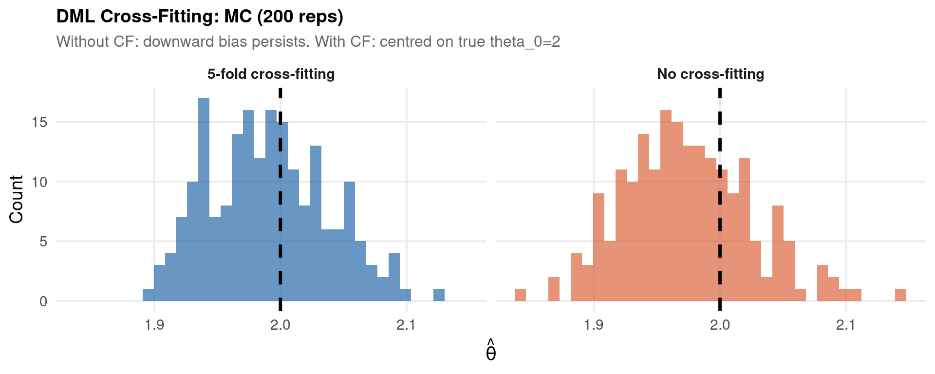
Cross-Fitting in Practice

Code
set.seed(14159)
n_mc_dml <- 200L
no_cf_mc <- cf_mc <- numeric(n_mc_dml)

for (i in seq_len(n_mc_dml)) {
  set.seed(i * 17 + 14159)
  Xm <- matrix(rnorm(n_dml*p_dml), nrow=n_dml)
  Dm <- 0.5*Xm[,1] - 0.4*Xm[,2] + 0.3*Xm[,3] + rnorm(n_dml)
  gm <- as.numeric(Xm[,1:5] %*% c(1.5,-1.2,0.8,-0.5,1.0))
  ym <- as.numeric(theta_true*Dm + gm + rnorm(n_dml))

  # No cross-fitting
  fg_nc <- cv.glmnet(Xm, ym, alpha=1, nfolds=3)
  fm_nc <- cv.glmnet(Xm, Dm, alpha=1, nfolds=3)
  yr_nc <- ym - predict(fg_nc, Xm, s="lambda.min")
  dr_nc <- Dm - predict(fm_nc, Xm, s="lambda.min")
  no_cf_mc[i] <- coef(lm(yr_nc ~ dr_nc))["dr_nc"]

  # 5-fold CF
  fls <- sample(rep(1:5, length.out=n_dml))
  yr_cf <- dr_cf <- numeric(n_dml)
  for (k in 1:5) {
    tr2 <- fls!=k; te2 <- fls==k
    fgk <- cv.glmnet(Xm[tr2,], ym[tr2], alpha=1, nfolds=3)
    fmk <- cv.glmnet(Xm[tr2,], Dm[tr2], alpha=1, nfolds=3)
    yr_cf[te2] <- ym[te2] - predict(fgk, Xm[te2,], s="lambda.min")
    dr_cf[te2] <- Dm[te2] - predict(fmk, Xm[te2,], s="lambda.min")
  }
  cf_mc[i] <- coef(lm(yr_cf ~ dr_cf))["dr_cf"]
}

tibble(theta=c(no_cf_mc, cf_mc),
       Method=rep(c("No cross-fitting","5-fold cross-fitting"), each=n_mc_dml)) %>%
  ggplot() +
    aes(theta, fill=Method) +
    geom_histogram(alpha=0.65, bins=35, position="identity") +
    geom_vline(xintercept=theta_true, linewidth=1.2, linetype="dashed") +
    scale_fill_manual(values=c("No cross-fitting"=col_accent,
                                "5-fold cross-fitting"=col_main)) +
    facet_wrap(~Method) +
    labs(x=expression(hat(theta)), y="Count",
         title=sprintf("DML Cross-Fitting: MC (%d reps)", n_mc_dml),
         subtitle="Without CF: downward bias persists. With CF: centred on true theta_0=2",
         fill=NULL) +
    theme_lecture + theme(legend.position="none")

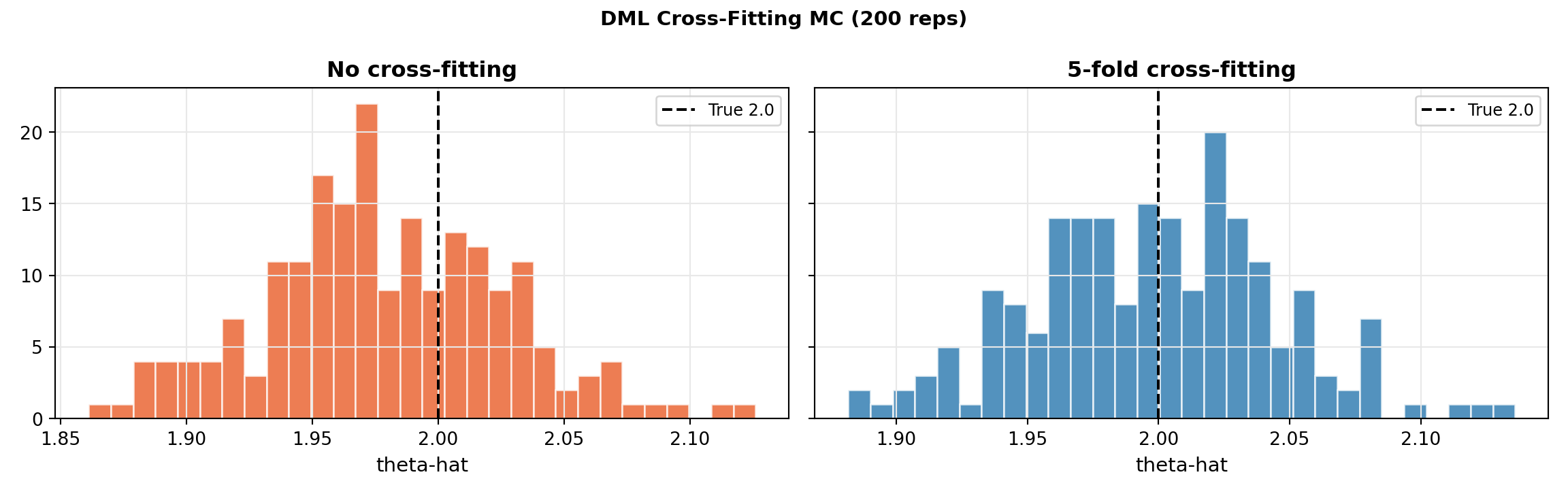
Code
import numpy as np, matplotlib.pyplot as plt
from sklearn.linear_model import LassoCV
from sklearn.model_selection import KFold

rng3 = np.random.default_rng(14159)
n_mc_d, n_d, p_d, th_tr = 200, 500, 50, 2.0
no_cf_r, cf_r = [], []

for rep in range(n_mc_d):
    Xm = rng3.standard_normal((n_d, p_d))
    Dm = 0.5*Xm[:,0]-0.4*Xm[:,1]+0.3*Xm[:,2]+rng3.normal(0,1,n_d)
    gm = Xm[:,:5]@np.array([1.5,-1.2,0.8,-0.5,1.0])
    ym = th_tr*Dm+gm+rng3.normal(0,1,n_d)

    fg=LassoCV(cv=3,max_iter=2000).fit(Xm,ym)
    fm=LassoCV(cv=3,max_iter=2000).fit(Xm,Dm)
    yr_nc=ym-fg.predict(Xm); dr_nc=Dm-fm.predict(Xm)
    no_cf_r.append(np.dot(dr_nc,yr_nc)/np.dot(dr_nc,dr_nc))

    yr_cf, dr_cf = np.zeros(n_d), np.zeros(n_d)
    for tr,te in KFold(5,shuffle=True,random_state=rep).split(Xm):
        fgk=LassoCV(cv=3,max_iter=2000).fit(Xm[tr],ym[tr])
        fmk=LassoCV(cv=3,max_iter=2000).fit(Xm[tr],Dm[tr])
        yr_cf[te]=ym[te]-fgk.predict(Xm[te]); dr_cf[te]=Dm[te]-fmk.predict(Xm[te])
    cf_r.append(np.dot(dr_cf,yr_cf)/np.dot(dr_cf,dr_cf))

fig,axes=plt.subplots(1,2,figsize=(12,3.8),sharey=True)
for ax,vals,label,col in zip(axes,[no_cf_r,cf_r],
    ["No cross-fitting","5-fold cross-fitting"],["#e8521a","#1a6ea8"]):
    ax.hist(vals,bins=30,color=col,alpha=0.75,edgecolor="white")
    ax.axvline(th_tr,color="black",ls="--",lw=1.5,label=f"True {th_tr}")
    ax.set_xlabel("theta-hat",fontsize=11); ax.set_title(label,fontweight="bold")
    ax.legend(fontsize=9); ax.grid(True,color="#e8e8e8")
fig.suptitle(f"DML Cross-Fitting MC ({n_mc_d} reps)",fontsize=11,fontweight="bold")
fig.tight_layout(); plt.show()

Code
print(f"No CF mean: {np.mean(no_cf_r):.4f}  CF mean: {np.mean(cf_r):.4f}  True: {th_tr}")
No CF mean: 1.9791  CF mean: 1.9981  True: 2.0

Nuisance Learners — RF, Boosting, Neural Nets

DML accepts any learner that fits the nuisances at rate \(o(n^{-1/4})\) — choose by out-of-fold fit:

  • Random forests — automatic interactions and nonlinearity, little tuning; the robust default
  • Boosted trees (XGBoost) — usually the best out-of-fold fit; tune depth and learning rate
  • Neural nets — flexible but data-hungry; at moderate \(n\) they often miss the rate condition (watch the table below)
  • Splines / GAMs (mgcv) — smooth low-dimensional nonlinearity; excellent when only a few continuous controls matter
  • Lasso / Ridge — the regularisation route (previous slides); best under approximate sparsity
Code
dml_estimate <- function(X, y, D, learner=c("lasso","ridge","rf","xgb","nnet"), K=5L) {
  learner <- match.arg(learner)
  folds <- sample(rep(1:K, length.out=nrow(X)))
  y_r <- D_r <- numeric(nrow(X))
  for (k in seq_len(K)) {
    tr <- folds!=k; te <- folds==k
    if (learner %in% c("lasso","ridge")) {
      al <- if(learner=="lasso") 1 else 0
      fg <- cv.glmnet(X[tr,], y[tr], alpha=al, nfolds=5)
      fm <- cv.glmnet(X[tr,], D[tr], alpha=al, nfolds=5)
      y_r[te] <- y[te]-predict(fg,X[te,],s="lambda.min")
      D_r[te] <- D[te]-predict(fm,X[te,],s="lambda.min")
    } else if (learner=="rf") {
      fg <- ranger(y~., data=data.frame(y=y[tr],X[tr,]), num.trees=200, min.node.size=5)
      fm <- ranger(D~., data=data.frame(D=D[tr],X[tr,]), num.trees=200, min.node.size=5)
      y_r[te] <- y[te]-predict(fg,data=data.frame(X[te,]))$predictions
      D_r[te] <- D[te]-predict(fm,data=data.frame(X[te,]))$predictions
    } else if (learner=="xgb") {
      fg <- xgb.train(list(objective="reg:squarederror",max_depth=3,eta=0.1),
                      xgb.DMatrix(X[tr,],label=y[tr]),nrounds=100,verbose=0)
      fm <- xgb.train(list(objective="reg:squarederror",max_depth=3,eta=0.1),
                      xgb.DMatrix(X[tr,],label=D[tr]),nrounds=100,verbose=0)
      y_r[te] <- y[te]-predict(fg,xgb.DMatrix(X[te,]))
      D_r[te] <- D[te]-predict(fm,xgb.DMatrix(X[te,]))
    } else {
      Xs_tr <- scale(X[tr,])
      Xs_te <- scale(X[te,], center=attr(Xs_tr,"scaled:center"),
                             scale=attr(Xs_tr,"scaled:scale"))
      fg <- nnet(Xs_tr, y[tr], size=8, decay=0.5, linout=TRUE, maxit=500, trace=FALSE)
      fm <- nnet(Xs_tr, D[tr], size=8, decay=0.5, linout=TRUE, maxit=500, trace=FALSE)
      y_r[te] <- y[te]-predict(fg,Xs_te)
      D_r[te] <- D[te]-predict(fm,Xs_te)
    }
  }
  fit <- lm(y_r~D_r)
  c(theta=unname(coef(fit)["D_r"]), se=sqrt(vcovHC(fit,"HC3")["D_r","D_r"]))
}

set.seed(14159)
res_nl <- NULL
for (l in c("lasso","ridge","rf","xgb","nnet")) {
  e <- dml_estimate(X_dml, y_dml, D_dml, learner=l)
  covered <- e["theta"]-1.96*e["se"] <= theta_true & theta_true <= e["theta"]+1.96*e["se"]
  res_nl <- rbind(res_nl, data.frame(
    Learner=toupper(l), theta=round(e[["theta"]],4), SE=round(e[["se"]],4),
    CI=sprintf("[%.4f, %.4f]", e["theta"]-1.96*e["se"], e["theta"]+1.96*e["se"]),
    Covered=ifelse(covered, "YES", "NO")))
}
cat(sprintf("DML nuisance learner comparison (true theta_0 = %.1f)\n", theta_true))
DML nuisance learner comparison (true theta_0 = 2.0)
Code
print(res_nl, row.names=FALSE)
 Learner  theta     SE               CI Covered
   LASSO 2.0815 0.0441 [1.9951, 2.1680]     YES
   RIDGE 2.0755 0.0422 [1.9927, 2.1583]     YES
      RF 2.4719 0.0721 [2.3306, 2.6132]      NO
     XGB 2.0134 0.0541 [1.9075, 2.1194]     YES
    NNET 1.3180 0.0956 [1.1307, 1.5053]      NO
Code
cat("Note: the neural net misses the o(n^-1/4) rate at n=500, p=50 - theta is attenuated. See Diagnostics.\n")
Note: the neural net misses the o(n^-1/4) rate at n=500, p=50 - theta is attenuated. See Diagnostics.
Code
import warnings; warnings.filterwarnings("ignore")
import numpy as np
from sklearn.linear_model import LassoCV, RidgeCV
from sklearn.ensemble import RandomForestRegressor
from sklearn.neural_network import MLPRegressor
from sklearn.preprocessing import StandardScaler
from sklearn.pipeline import make_pipeline
import xgboost as xgb_mod
from sklearn.model_selection import KFold

def dml_py(X, y, D, learner='lasso', K=5):
    kf = KFold(K, shuffle=True, random_state=14159)
    yr, Dr = np.zeros(len(y)), np.zeros(len(D))
    for tr, te in kf.split(X):
        if learner=='lasso':
            Mg=LassoCV(cv=5,max_iter=3000).fit(X[tr],y[tr])
            Mm=LassoCV(cv=5,max_iter=3000).fit(X[tr],D[tr])
        elif learner=='ridge':
            Mg=RidgeCV(cv=5).fit(X[tr],y[tr])
            Mm=RidgeCV(cv=5).fit(X[tr],D[tr])
        elif learner=='rf':
            Mg=RandomForestRegressor(200,min_samples_leaf=5,random_state=42).fit(X[tr],y[tr])
            Mm=RandomForestRegressor(200,min_samples_leaf=5,random_state=42).fit(X[tr],D[tr])
        elif learner=='xgb':
            Mg=xgb_mod.XGBRegressor(max_depth=3,learning_rate=0.1,n_estimators=100,
                                     random_state=42,verbosity=0).fit(X[tr],y[tr])
            Mm=xgb_mod.XGBRegressor(max_depth=3,learning_rate=0.1,n_estimators=100,
                                     random_state=42,verbosity=0).fit(X[tr],D[tr])
        else:
            Mg=make_pipeline(StandardScaler(), MLPRegressor(hidden_layer_sizes=(8,),
                 alpha=0.5, max_iter=2000, random_state=42)).fit(X[tr],y[tr])
            Mm=make_pipeline(StandardScaler(), MLPRegressor(hidden_layer_sizes=(8,),
                 alpha=0.5, max_iter=2000, random_state=42)).fit(X[tr],D[tr])
        yr[te]=y[te]-Mg.predict(X[te]); Dr[te]=D[te]-Mm.predict(X[te])
    th = np.dot(Dr,yr)/np.dot(Dr,Dr)
    psi = Dr*(yr-th*Dr)
    se = ((Dr**2).mean()**(-2)*(psi**2).mean()/len(y))**0.5
    return th, se

lines = [f"{'Learner':<8} {'theta':>8} {'SE':>8} {'95% CI':>24} {'Covered':>8}", "-"*64]
for l in ['lasso','ridge','rf','xgb','nnet']:
    th, se = dml_py(X_dml, y_dml, D_dml, learner=l)
    lo, hi = th-1.96*se, th+1.96*se
    cov = "YES" if lo<=theta_true<=hi else "NO"
    lines.append(f"{l.upper():<8} {th:>8.4f} {se:>8.4f} [{lo:>8.4f}, {hi:>8.4f}] {cov:>8}")
import sys; sys.stdout.write("\n".join(lines) + "\n"); sys.stdout.flush()
Learner     theta       SE                   95% CI  Covered
----------------------------------------------------------------
LASSO      2.0493   0.0478 [  1.9557,   2.1430]      YES
RIDGE      2.0400   0.0460 [  1.9497,   2.1302]      YES
RF         2.2009   0.0667 [  2.0702,   2.3315]       NO
XGB        2.0198   0.0663 [  1.8898,   2.1498]      YES
NNET       1.8331   0.0821 [  1.6722,   1.9941]       NO
411

DML Diagnostics & Limitations

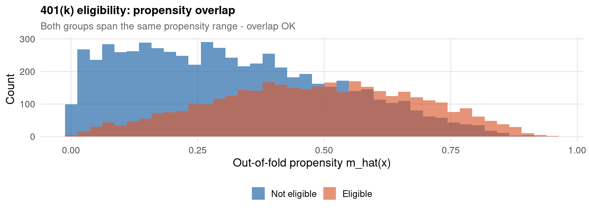
Residualisation needs comparable units: if \(\hat{m}(\mathbf{x}) \approx 0\) or \(\approx 1\) for binary \(D\), some covariate cells contain only treated or only controls.

\[\text{Var}(\hat\theta) \;\propto\; \frac{1}{\mathbb{E}\big[m(\mathbf{x})(1-m(\mathbf{x}))\big]}\]

  • always plot the propensity distribution by treatment group
  • standard fix: trim observations with \(\hat{m} \notin [0.02, 0.98]\)

After partialling-out, all identifying variation lives in \(\tilde{D} = D - \hat{m}(\mathbf{x})\):

\[\text{Var}(\tilde{D}) \approx 0 \;\Rightarrow\; D \text{ is (almost) a deterministic function of } \mathbf{x}\]

  • SE of \(\hat\theta\) explodes; tiny nuisance errors dominate the estimate
  • report \(\text{Var}(\tilde{D})\) (or the first-stage partial \(R^2\)) alongside \(\hat\theta\)

Orthogonality protects against small nuisance errors — it cannot rescue a learner that fails the rate condition:

\[\|\hat g - g_0\| \cdot \|\hat m - m_0\| = o(n^{-1/2}) \quad \text{needed}\]

  • check out-of-fold \(R^2\) of both nuisances; a learner that predicts poorly out-of-fold transmits bias
  • the neural-net row on the previous slide is exactly this failure: at \(n=500\), \(p=50\) the net misses the rate and \(\hat\theta\) is attenuated
  • the fold split is random — rerun with several splits (n_rep in DoubleML) and report the median
  • asymptotics kick in slowly: at small \(n\), DML inherits the combined noise of two ML fits plus a regression
  • good practice: report naive OLS, DML with two different learners, and the diagnostics above in one table
Code
data("pension", package="hdm")
df_dg <- pension %>%
  select(net_tfa, e401, age, inc, fsize, educ, marr, twoearn, db, pira, hown) %>%
  mutate(age2=age^2, inc2=inc^2, fsize2=fsize^2, educ2=educ^2)
X_dg <- as.matrix(df_dg[, setdiff(names(df_dg), c("net_tfa","e401"))])
y_dg <- df_dg$net_tfa; D_dg <- df_dg$e401

set.seed(14159)
folds_dg <- sample(rep(1:5, length.out=nrow(df_dg)))
m_hat <- g_hat <- numeric(nrow(df_dg))
for (k in 1:5) {
  tr <- folds_dg!=k; te <- folds_dg==k
  fm <- ranger(D~., data=data.frame(D=D_dg[tr], X_dg[tr,]), num.trees=200, seed=14159)
  fg <- ranger(y~., data=data.frame(y=y_dg[tr], X_dg[tr,]), num.trees=200, seed=14159)
  m_hat[te] <- predict(fm, data=data.frame(X_dg[te,]))$predictions
  g_hat[te] <- predict(fg, data=data.frame(X_dg[te,]))$predictions
}
r2_m <- 1 - mean((D_dg-m_hat)^2)/var(D_dg)
r2_g <- 1 - mean((y_dg-g_hat)^2)/var(y_dg)
cat(sprintf("Out-of-fold R2:  m(x) [propensity] = %.3f   g(x) [outcome] = %.3f\n",
            r2_m, r2_g))
Out-of-fold R2:  m(x) [propensity] = 0.120   g(x) [outcome] = 0.250
Code
cat(sprintf("Var(D_tilde) = %.3f   overlap: %.1f%% of m_hat in [0.02, 0.98]\n",
            var(D_dg - m_hat), 100*mean(m_hat > 0.02 & m_hat < 0.98)))
Var(D_tilde) = 0.205   overlap: 98.1% of m_hat in [0.02, 0.98]
Code
data.frame(m_hat = m_hat, group = factor(D_dg, labels=c("Not eligible","Eligible"))) %>%
  ggplot() +
    aes(m_hat, fill=group) +
    geom_histogram(alpha=0.65, bins=40, position="identity") +
    scale_fill_manual(values=c("Not eligible"="#185FA5", "Eligible"="#D85A30")) +
    labs(x="Out-of-fold propensity m_hat(x)", y="Count", fill=NULL,
         title="401(k) eligibility: propensity overlap",
         subtitle="Both groups span the same propensity range - overlap OK") +
    theme_lecture

Application — Minimum Wage: Card & Krueger with DML

The design: New Jersey raised its minimum wage from $4.25 to $5.05 in April 1992; eastern Pennsylvania did not. Outcome: change in full-time-equivalent employment at 410 fast-food stores (Card & Krueger 1994). DML residualises the store-level covariates with a random forest instead of assuming linear controls.

Code
ff_raw <- read.csv("../data/causal-ml-fastfood-raw.csv")
fte  <- ff_raw$empft  + ff_raw$nmgrs  + 0.5*ff_raw$emppt
fte2 <- ff_raw$empft2 + ff_raw$nmgrs2 + 0.5*ff_raw$emppt2
cat(sprintf("Card-Krueger DiD, full sample: %.2f FTE\n",
            mean((fte2-fte)[ff_raw$state==1], na.rm=TRUE) -
            mean((fte2-fte)[ff_raw$state==0], na.rm=TRUE)))
Card-Krueger DiD, full sample: 2.75 FTE
Code
ff <- read.csv("../data/causal-ml-fastfood.csv")   # created by causal-ml-data.R

naive_mw <- lm(dfte ~ nj, data=ff)
cat(sprintf("Analysis sample (n=%d) simple diff: %.3f (SE %.3f)\n", nrow(ff),
            coef(naive_mw)["nj"], sqrt(vcovHC(naive_mw,"HC1")["nj","nj"])))
Analysis sample (n=361) simple diff: 2.303 (SE 1.369)
Code
set.seed(14159)
X_mw <- as.matrix(ff[, setdiff(names(ff), c("dfte","nj"))])
folds_mw <- sample(rep(1:5, length.out=nrow(ff)))
yr_mw <- Dr_mw <- numeric(nrow(ff))
for (k in 1:5) {
  tr <- folds_mw!=k; te <- folds_mw==k
  fg <- ranger(y~., data=data.frame(y=ff$dfte[tr], X_mw[tr,]),
               num.trees=500, min.node.size=5, seed=14159)
  fm <- ranger(D~., data=data.frame(D=ff$nj[tr], X_mw[tr,]),
               num.trees=500, min.node.size=5, seed=14159)
  yr_mw[te] <- ff$dfte[te] - predict(fg, data=data.frame(X_mw[te,]))$predictions
  Dr_mw[te] <- ff$nj[te]   - predict(fm, data=data.frame(X_mw[te,]))$predictions
}
dml_mw <- lm(yr_mw ~ Dr_mw)
cat(sprintf("DML-RF effect of NJ minimum wage: %.3f (SE %.3f)\n",
            coef(dml_mw)["Dr_mw"], sqrt(vcovHC(dml_mw,"HC3")["Dr_mw","Dr_mw"])))
DML-RF effect of NJ minimum wage: 2.045 (SE 1.352)
Code
import pandas as pd, numpy as np
import statsmodels.api as sm
from sklearn.ensemble import RandomForestRegressor
from sklearn.model_selection import KFold

ff = pd.read_csv("../data/causal-ml-fastfood.csv")
y_mw = ff["dfte"].values
D_mw = ff["nj"].values
X_mw = ff.drop(columns=["dfte","nj"]).values

naive = sm.OLS(y_mw, sm.add_constant(D_mw)).fit(cov_type="HC1")

yr, Dr = np.zeros(len(ff)), np.zeros(len(ff))
for tr, te in KFold(5, shuffle=True, random_state=14159).split(X_mw):
    fg = RandomForestRegressor(n_estimators=500, min_samples_leaf=5,
                               random_state=14159).fit(X_mw[tr], y_mw[tr])
    fm = RandomForestRegressor(n_estimators=500, min_samples_leaf=5,
                               random_state=14159).fit(X_mw[tr], D_mw[tr])
    yr[te] = y_mw[te] - fg.predict(X_mw[te])
    Dr[te] = D_mw[te] - fm.predict(X_mw[te])
th_mw = np.dot(Dr, yr) / np.dot(Dr, Dr)
psi_mw = Dr*(yr - th_mw*Dr)
se_mw = ((Dr**2).mean()**(-2) * (psi_mw**2).mean() / len(ff))**0.5

out = (f"Analysis sample n = {len(ff)}\n"
       f"Simple diff NJ-PA: {naive.params[1]:.3f} (SE {naive.bse[1]:.3f})\n"
       f"DML-RF effect:     {th_mw:.3f} (SE {se_mw:.3f})")
import sys; sys.stdout.write(out + "\n"); sys.stdout.flush()
Analysis sample n = 361
Simple diff NJ-PA: 2.303 (SE 1.369)
DML-RF effect:     1.709 (SE 1.327)
96
Code
quietly import delimited "../data/causal-ml-fastfood.csv", clear
quietly destring _all, replace
quietly regress dfte nj, robust
display "Simple diff NJ-PA: " %6.3f _b[nj] " (SE " %5.3f _se[nj] ")"
pdslasso dfte nj (bk-bonus), robust
Simple diff NJ-PA:  2.303 (SE 1.369)

1.  (PDS/CHS) Selecting HD controls for dep var dfte...
Selected: 
2.  (PDS/CHS) Selecting HD controls for exog regressor nj...
Selected: 


Estimation results:

Specification:
Regularization method:                 lasso
Penalty loadings:                      heteroskedastic
Number of observations:                361
Exogenous (1):                         nj
High-dim controls (9):                 bk kfc roys co_owned wage_st hrsopen
                                       open nregs bonus
Selected controls (0):
Unpenalized controls (1):              _cons

Structural equation:

OLS using CHS lasso-orthogonalized vars
------------------------------------------------------------------------------
             |               Robust
        dfte | Coefficient  std. err.      z    P>|z|     [95% conf. interval]
-------------+----------------------------------------------------------------
          nj |     2.3031   1.364796     1.69   0.092    -.3718504     4.97805
------------------------------------------------------------------------------

OLS using CHS post-lasso-orthogonalized vars
------------------------------------------------------------------------------
             |               Robust
        dfte | Coefficient  std. err.      z    P>|z|     [95% conf. interval]
-------------+----------------------------------------------------------------
          nj |     2.3031   1.364796     1.69   0.092    -.3718504     4.97805
------------------------------------------------------------------------------

OLS with PDS-selected variables and full regressor set
------------------------------------------------------------------------------
             |               Robust
        dfte | Coefficient  std. err.      z    P>|z|     [95% conf. interval]
-------------+----------------------------------------------------------------
          nj |     2.3031   1.364796     1.69   0.092    -.3718504     4.97805
       _cons |  -2.145833   1.280151    -1.68   0.094    -4.654883    .3632164
------------------------------------------------------------------------------
Standard errors and test statistics valid for the following variables only:
    nj
------------------------------------------------------------------------------

Two Routes to Valid Inference: Double-Selection vs Partialling-Out

Both routes solve the post-model-selection inference problem (Leeb & Pötscher 2005):

  • naive post-Lasso confidence intervals have badly distorted coverage when \(D\) and \(\mathbf{x}\) are correlated
  • both routes restore valid inference with conventional standard errors

Double-Selection Lasso (Belloni, Chernozhukov & Hansen 2014):

\[y_i = \theta D_i + \mathbf{x}_i'\boldsymbol\beta + e_i, \qquad D_i = \mathbf{x}_i'\boldsymbol\gamma + v_i\]

  1. Lasso of \(D\) on \(\mathbf{x}\) → selected set \(X_1\)
  2. Lasso of \(y\) on \(\mathbf{x}\) → selected set \(X_2\)
  3. OLS of \(y\) on \((D, X_1 \cup X_2)\) — the union of selected controls
  4. Conventional heteroskedastic SE on \(\hat\theta^{DS}\)

Post-Regularization (Partialling-Out) Lasso (Chernozhukov, Hansen & Spindler 2015):

\[y_i - \mathbb{E}[y_i|\mathbf{x}_i] = \big(D_i - \mathbb{E}[D_i|\mathbf{x}_i]\big)\theta + e_i\]

  1. Lasso of \(D\) on \(\mathbf{x}\) → residual \(\hat{v}_i = D_i - \mathbf{x}_i'\hat{\boldsymbol\gamma}\)
  2. Lasso of \(y\) on \(\mathbf{x}\) → residual \(\hat{u}_i = y_i - \mathbf{x}_i'\hat{\boldsymbol\eta}\)
  3. OLS of \(\hat{u}\) on \(\hat{v}\)\(\hat\theta^{PR}\) (this is Robinson 1988 with Lasso nuisance)

The trade-off (Hansen §29.21):

Double-Selection Partialling-Out
Controls used Union \(X_1 \cup X_2\) Separate for \(y\) and \(D\)
Property More robust (less bias) More efficient (parsimony)
Asymptotics Harder to derive Easier (rate manipulation only)
Stata dsregress poregress
R hdm hdm

DML — Results: What to Report

Item What to state Example
Model Partially linear, IV, interactive “Partially linear model, Robinson (1988)”
Nuisance learner Method + CV “Lasso, 5-fold cross-fitting”
\(\hat\theta\) Point + SE + CI “2.012 (SE 0.089, 95% CI [1.838, 2.186])”
Robustness Multiple learners “Robust across Lasso, Ridge, RF, XGBoost”
Bias of naive OLS For contrast “Naive OLS: 2.31 (bias +0.31)”
Code
cat("````latex\n")

```{.r .cell-code  code-fold="true" code-summary="Code"}
cat("%% DML estimator\n\\begin{equation}\n")
```

%% DML estimator
\begin{equation}

```{.r .cell-code  code-fold="true" code-summary="Code"}
cat("  \\hat\\theta^{\\text{DML}} = \\left(\\sum_{i\\in I^c}\\tilde{D}_i^2\\right)^{-1}\\sum_{i\\in I^c}\\tilde{D}_i\\tilde{y}_i\n")
```

  \hat\theta^{\text{DML}} = \left(\sum_{i\in I^c}\tilde{D}_i^2\right)^{-1}\sum_{i\in I^c}\tilde{D}_i\tilde{y}_i

```{.r .cell-code  code-fold="true" code-summary="Code"}
cat("  \\quad\\tilde{y}_i = y_i - \\hat{g}(\\mathbf{x}_i),\\quad\\tilde{D}_i = D_i - \\hat{m}(\\mathbf{x}_i)\n")
```

  \quad\tilde{y}_i = y_i - \hat{g}(\mathbf{x}_i),\quad\tilde{D}_i = D_i - \hat{m}(\mathbf{x}_i)

```{.r .cell-code  code-fold="true" code-summary="Code"}
cat("  \\label{eq:dml}\n\\end{equation}\n````\n")
```

  \label{eq:dml}
\end{equation}

Software — DoubleML, doubleml, ddml

Same partially linear model, three native implementations — the 401(k) eligibility effect once more. R and Python use random-forest nuisance, Stata’s ddml uses rigorous Lasso; all three cross-fit with \(K=5\).

Code
lgr::get_logger("mlr3")$set_threshold("warn")
data("pension", package="hdm")
df_sw <- pension %>%
  select(net_tfa, e401, age, inc, fsize, educ, marr, twoearn, db, pira, hown) %>%
  mutate(age2=age^2, inc2=inc^2, fsize2=fsize^2, educ2=educ^2)
set.seed(14159)
dml_data <- double_ml_data_from_data_frame(df_sw, y_col="net_tfa", d_cols="e401")
plr_sw <- DoubleMLPLR$new(dml_data,
            ml_l = lrn("regr.ranger", num.trees=200, min.node.size=5),
            ml_m = lrn("regr.ranger", num.trees=200, min.node.size=5),
            n_folds = 5)
plr_sw$fit()
plr_sw$summary()
Estimates and significance testing of the effect of target variables
     Estimate. Std. Error t value Pr(>|t|)    
e401      8896       1281   6.942 3.86e-12 ***
---
Signif. codes:  0 '***' 0.001 '**' 0.01 '*' 0.05 '.' 0.1 ' ' 1
Code
import warnings; warnings.filterwarnings("ignore")
import pandas as pd, numpy as np
import doubleml as dml
from sklearn.ensemble import RandomForestRegressor

df_sw = pd.read_csv("../data/causal-ml-pension.csv")
np.random.seed(14159)
data_sw = dml.DoubleMLData(df_sw, y_col="net_tfa", d_cols="e401")
plr_sw = dml.DoubleMLPLR(data_sw,
           RandomForestRegressor(n_estimators=200, min_samples_leaf=5, random_state=14159),
           RandomForestRegressor(n_estimators=200, min_samples_leaf=5, random_state=14159),
           n_folds=5)
plr_fitted = plr_sw.fit()
out = plr_sw.summary.round(2).to_string()
import sys; sys.stdout.write(out + "\n"); sys.stdout.flush()
         coef  std err     t  P>|t|    2.5 %    97.5 %
e401  9360.26  1360.29  6.88    0.0  6694.15  12026.37
110
Code
quietly import delimited "../data/causal-ml-pension.csv", clear
quietly destring _all, replace
set seed 14159
ddml init partial, kfolds(5)
ddml E[Y|X]: rlasso net_tfa age-educ2
ddml E[D|X]: rlasso e401 age-educ2
quietly ddml crossfit
ddml estimate, robust
Learner Y1_rlasso added successfully.

Learner D1_rlasso added successfully.


Model:                  partial, crossfit folds k=5, resamples r=1
Mata global (mname):    m0
Dependent variable (Y): net_tfa
 net_tfa learners:      Y1_rlasso
D equations (1):        e401
 e401 learners:         D1_rlasso

DDML estimation results:
spec  r     Y learner     D learner         b        SE 
   1  1     Y1_rlasso     D1_rlasso  8068.775 (1475.318)

DDML model
y-E[y|X]  = y-Y1_rlasso_1                          Number of obs   =      9915
D-E[D|X]  = D-D1_rlasso_1 
------------------------------------------------------------------------------
             |               Robust
     net_tfa | Coefficient  std. err.      z    P>|z|     [95% conf. interval]
-------------+----------------------------------------------------------------
        e401 |   8068.775   1475.318     5.47   0.000     5177.205    10960.35
       _cons |   59.30118   550.9992     0.11   0.914    -1020.637     1139.24
------------------------------------------------------------------------------

Part III — Heterogeneous Treatment Effects

CATE · Causal Forests · Meta-Learners · Policy Learning

Why Heterogeneity Matters

  • The ATE answers “what is the average effect?” — the CATE answers “for whom?
  • Policy targeting: treat where the effect is largest per euro spent
  • Welfare analysis: an average near zero can hide large gains for some and losses for others
  • Optimal assignment: who gets the training slot, the subsidy, the eligibility?

\[\tau(\mathbf{x}) = \mathbb{E}[Y_i(1) - Y_i(0) \mid \mathbf{X}_i = \mathbf{x}]\]

The ATE is one moment of the effect distribution:

\[\text{ATE} = \mathbb{E}[\tau(\mathbf{X})], \qquad \text{Var}\big(\tau(\mathbf{X})\big) > 0 \iff \text{systematic heterogeneity}\]

  • a positive ATE with wide \(\tau(\mathbf{x})\) dispersion argues for targeted rather than universal treatment
  • reporting only the ATE discards the policy-relevant variation
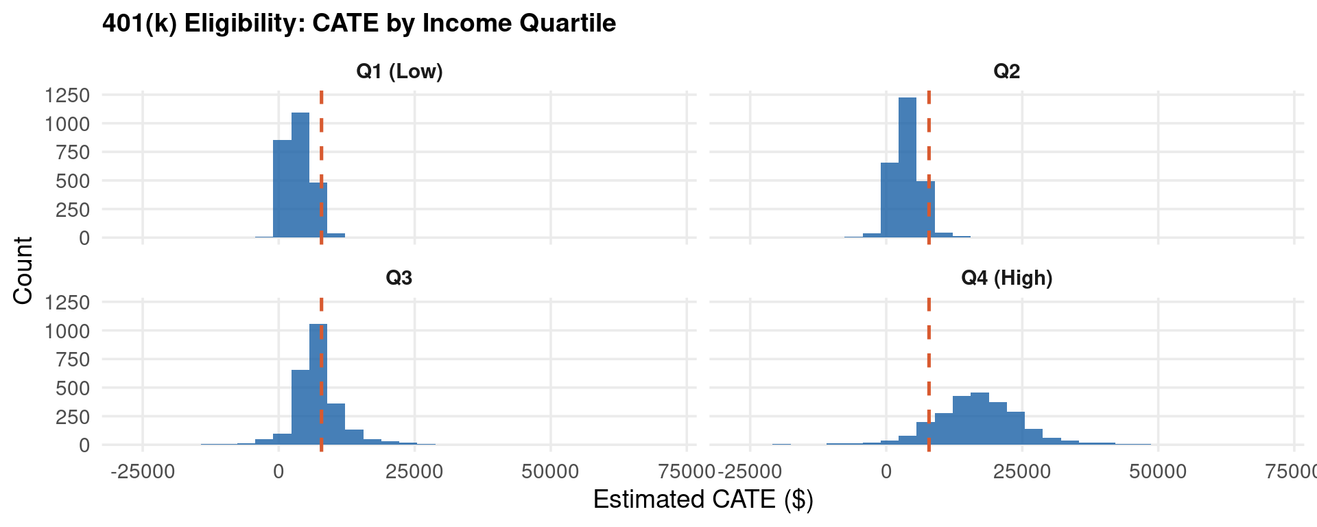
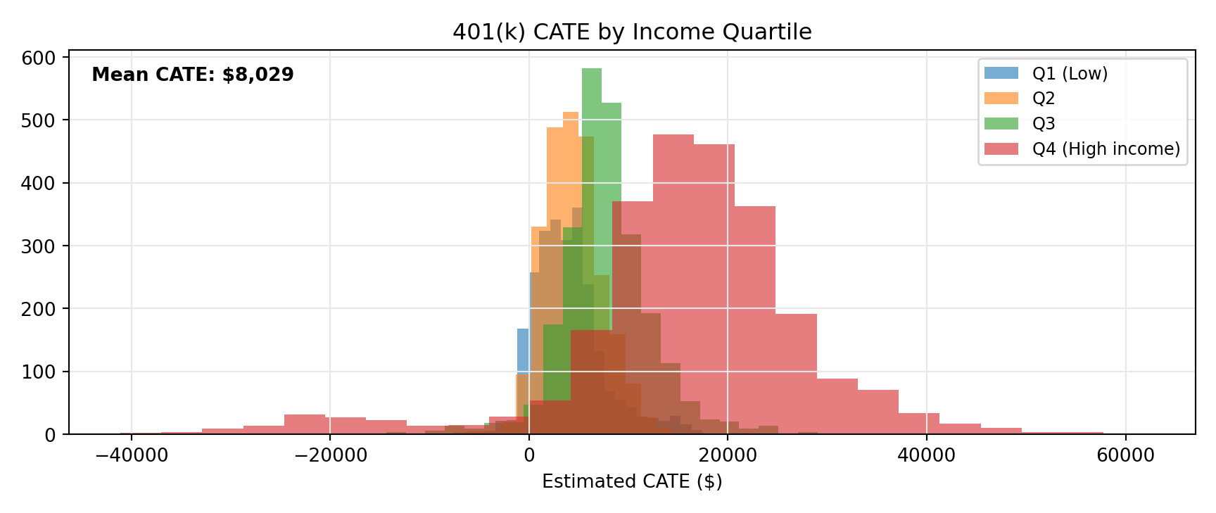
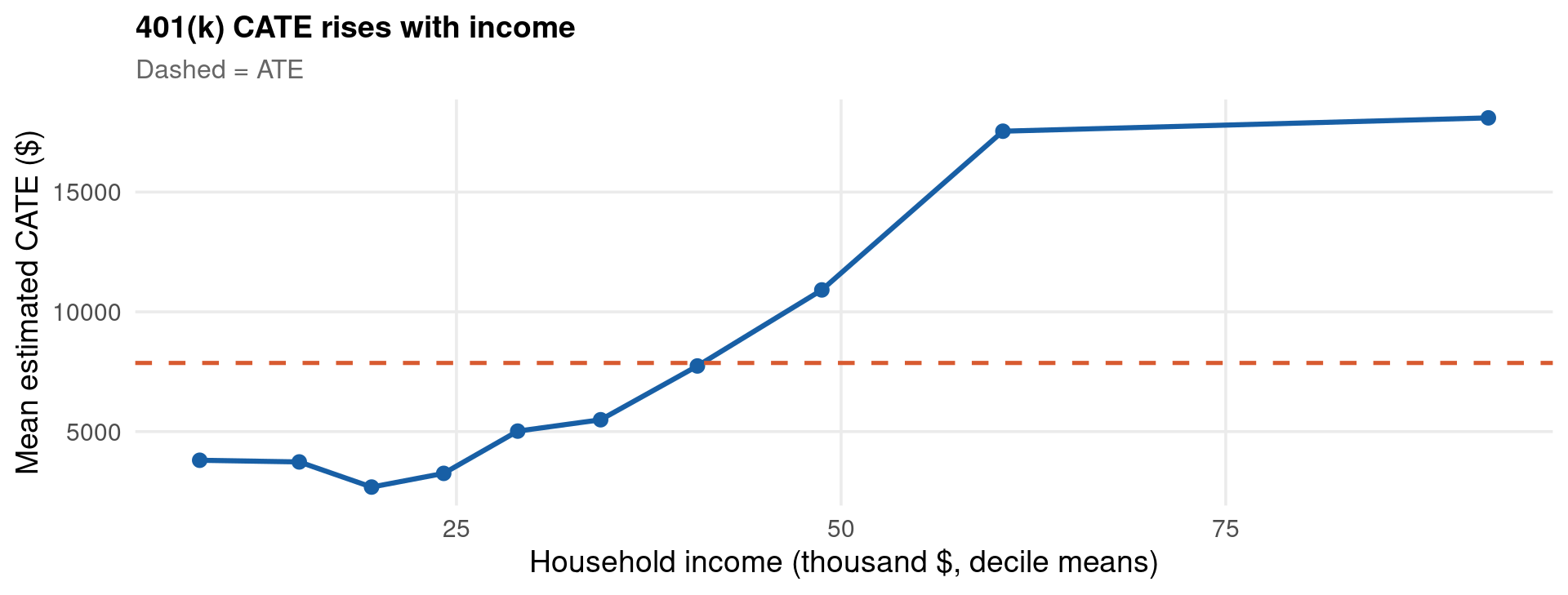
  • 401(k) eligibility: savings response rises steeply with income (this part)
  • class size: gains concentrate among disadvantaged students (STAR, this part)
  • job training: returns differ by prior earnings history (NSW, this part)

CATE vs ITE

\[\tau_i = Y_i(1) - Y_i(0) \qquad \text{(ITE — individual treatment effect)}\]

\[\tau(\mathbf{x}) = \mathbb{E}[\tau_i \mid \mathbf{X}_i = \mathbf{x}] \qquad \text{(CATE — conditional average)}\]

  • \(\tau_i\) is never observed — one potential outcome is always missing
  • \(\tau(\mathbf{x})\) is identified under unconfoundedness and overlap

The CATE is the best approximation of the ITE given observables:

\[\text{Var}(\tau_i) = \underbrace{\text{Var}\big(\tau(\mathbf{X}_i)\big)}_{\text{explained by } \mathbf{X}} + \underbrace{\mathbb{E}\big[\text{Var}(\tau_i \mid \mathbf{X}_i)\big]}_{\text{invisible to any estimator}}\]

  • even a perfect CATE model cannot rank individuals within a covariate cell
  • richer \(\mathbf{X}\) → CATE closer to the ITE — but the second term never reaches zero in practice
  • CATE estimation is a regression problem on an unobserved outcome — that is why every estimator (forest, meta-learner) first constructs a proxy for \(\tau_i\)
  • inference targets: pointwise CIs for \(\tau(\mathbf{x})\), the best linear projection, or group ATEs — never individual \(\tau_i\)
  • report: the ATE, a heterogeneity test, and group-level CATEs with CIs

Application — 401(k) Eligibility: CATE

Code
data("pension", package="hdm")
X_pw_cols <- intersect(c("age","inc","income","fsize","educ","male","married","pira"),
                       names(pension))
if (all(c("inc","income") %in% X_pw_cols)) X_pw_cols <- setdiff(X_pw_cols,"income")
X_pw_cols <- setdiff(X_pw_cols,"net_tfa")
X_pw <- as.matrix(pension[,X_pw_cols]); Y_pw <- pension$net_tfa; W_pw <- pension$e401

set.seed(14159)
cf_pw <- causal_forest(X_pw, Y_pw, W_pw, num.trees=2000, honesty=TRUE, seed=14159)
ate_pw <- average_treatment_effect(cf_pw)
cat(sprintf("401(k) eligibility ATE: $%.0f  SE: $%.0f  CI: [$%.0f, $%.0f]\n",
            ate_pw["estimate"], ate_pw["std.err"],
            ate_pw["estimate"]-1.96*ate_pw["std.err"],
            ate_pw["estimate"]+1.96*ate_pw["std.err"]))
401(k) eligibility ATE: $7866  SE: $1160  CI: [$5592, $10139]
Code
tau_pw <- predict(cf_pw)$predictions
inc_col <- if("inc" %in% names(pension)) "inc" else "income"
pension %>% mutate(tau_hat=tau_pw, inc_q=ntile(.data[[inc_col]],4),
  inc_label=factor(inc_q, labels=c("Q1 (Low)","Q2","Q3","Q4 (High)"))) %>%
  ggplot() +
    aes(tau_hat) +
    geom_histogram(fill=col_main, alpha=0.8, bins=30) +
    facet_wrap(~inc_label) +
    geom_vline(xintercept=ate_pw["estimate"], colour=col_accent,
               linetype="dashed", linewidth=0.9) +
    labs(x="Estimated CATE ($)", y="Count",
         title="401(k) Eligibility: CATE by Income Quartile") +
    theme_lecture

Code
import pandas as pd, numpy as np, matplotlib.pyplot as plt
from econml.grf import CausalForest

# Real data: same 401(k) file as the R tab (hdm::pension)
df_a2 = pd.read_csv("../data/causal-ml-pension.csv")
feat_a2 = ["age","inc","fsize","educ","marr","pira"]
X_a2 = df_a2[feat_a2].values
W_a2 = df_a2["e401"].values
Y_a2 = df_a2["net_tfa"].values

cf = CausalForest(n_estimators=1000, min_samples_leaf=10,
                  honest=True, random_state=14159).fit(X_a2, W_a2, Y_a2)
tau_hat = cf.predict(X_a2).flatten()

inc_q  = pd.qcut(df_a2["inc"], 4, labels=False).values
labels = ["Q1 (Low)","Q2","Q3","Q4 (High income)"]
fig, ax = plt.subplots(figsize=(9,3.8))
for q, lbl in enumerate(labels):
    hcounts = ax.hist(tau_hat[inc_q==q], bins=25, alpha=0.6, label=lbl)
axopts = ax.set(xlabel="Estimated CATE ($)", title="401(k) CATE by Income Quartile")
ax.text(0.02, 0.92, f"Mean CATE: ${tau_hat.mean():,.0f}", transform=ax.transAxes,
        fontweight="bold")
ax.legend(fontsize=9); ax.grid(True, color="#e8e8e8")
plt.tight_layout(); plt.show()

Causal Forests — Theory

Causal Forest (Wager & Athey 2018): a nonparametric CATE estimator with pointwise asymptotic normality.

Each tree splits its sample in two: one half chooses the splits, the other estimates the leaf effects.

  • without honesty: leaf means overfit — the same data picks where to look and what to report
  • with honesty: leaf estimates are unbiased conditional on the tree structure — the key to valid CIs

Trees split to maximise heterogeneity of the treatment effect across children, not to predict \(Y\):

\[\max_{\text{split}} \; \frac{n_L n_R}{(n_L + n_R)^2} \big(\hat\tau_L - \hat\tau_R\big)^2\]

  • grf uses a gradient-based approximation of this criterion for speed
  • residualised outcomes \(Y - \hat{y}(\mathbf{x})\) and treatments \(W - \hat{w}(\mathbf{x})\) enter the splits — an orthogonalised forest (the DML idea again)

With honesty + subsampling (each tree sees a random fraction, without replacement):

\[\frac{\hat\tau(\mathbf{x}) - \tau(\mathbf{x})}{\sqrt{\widehat{\text{Var}}\big(\hat\tau(\mathbf{x})\big)}} \xrightarrow{d} \mathcal{N}(0, 1) \quad \text{pointwise}\]

  • the variance is estimable (infinitesimal jackknife) → pointwise confidence intervals
  • rates are slower than parametric — CIs are honest but wide in small samples

Causal Forests — Implementation

DGP 2 (from the setup): \(n = 500\), \(p = 5\), true CATE \(\tau(\mathbf{x}) = 2 + v_1\), selection into treatment through \(v_1, v_2\).

Code
cat(sprintf("DGP 2: n=%d, p=%d\n", nrow(df_cate), 5))
DGP 2: n=500, p=5
Code
cat(sprintf("True CATE: tau(x) = 2 + v1\n"))
True CATE: tau(x) = 2 + v1
Code
cat(sprintf("True ATE: %.3f\n", mean(df_cate$tau_true)))
True ATE: 1.984
Code
set.seed(14159)
X_cf <- as.matrix(df_cate[, paste0("v", 1:5)])
cf   <- causal_forest(X_cf, df_cate$y, df_cate$W,
                      num.trees=2000, honesty=TRUE, seed=14159)

ate <- average_treatment_effect(cf, target.sample="all")
cat(sprintf("CF ATE: %.4f  SE: %.4f  CI: [%.4f, %.4f]\n",
            ate["estimate"], ate["std.err"],
            ate["estimate"]-1.96*ate["std.err"],
            ate["estimate"]+1.96*ate["std.err"]))
CF ATE: 2.2238  SE: 0.1039  CI: [2.0201, 2.4274]
Code
import pandas as pd, numpy as np

# Same DGP 2 draw as the R tab (created by causal-ml-data.R)
df_cf2 = pd.read_csv("../data/causal-ml-dgp2.csv")
X_cf2 = df_cf2[[f"v{j}" for j in range(1, 6)]].values
W_cf2 = df_cf2["W"].values
Y_cf2 = df_cf2["y"].values
tau_true2 = df_cf2["tau_true"].values

from econml.grf import CausalForest
cf2 = CausalForest(n_estimators=2000, min_samples_leaf=5,
                    honest=True, random_state=14159).fit(X_cf2, W_cf2, Y_cf2)
tau_hat2 = cf2.predict(X_cf2).flatten()

out = (f"DGP: n={len(Y_cf2)}, p={X_cf2.shape[1]}\n"
       f"True ATE = E[tau(x)] = {tau_true2.mean():.4f}\n"
       f"Treatment share: {W_cf2.mean():.3f}\n"
       f"Causal Forest ATE: {tau_hat2.mean():.4f}  (true: {tau_true2.mean():.4f})\n"
       f"Cor(tau_hat, tau_true): {np.corrcoef(tau_hat2, tau_true2)[0,1]:.3f}")
import sys; sys.stdout.write(out + "\n"); sys.stdout.flush()
DGP: n=500, p=5
True ATE = E[tau(x)] = 1.9835
Treatment share: 0.498
Causal Forest ATE: 2.3964  (true: 1.9835)
Cor(tau_hat, tau_true): 0.955
141
Code
tau_hat_cf <- predict(cf, estimate.variance=TRUE)
tau_hat    <- tau_hat_cf$predictions
tau_se     <- sqrt(tau_hat_cf$variance.estimates)

cat(sprintf("Cor(tau_hat, tau_true): %.3f\n", cor(tau_hat, df_cate$tau_true)))
Cor(tau_hat, tau_true): 0.927
Code
cat(sprintf("RMSE(tau_hat, tau_true): %.4f\n", sqrt(mean((tau_hat-df_cate$tau_true)^2))))
RMSE(tau_hat, tau_true): 0.6232
Code
blp <- best_linear_projection(cf, X_cf)
cat("\nBest Linear Projection (tests heterogeneity):\n")

Best Linear Projection (tests heterogeneity):
Code
print(round(blp, 4))

Best linear projection of the conditional average treatment effect.
Confidence intervals are cluster- and heteroskedasticity-robust (HC3):

            Estimate Std. Error t value Pr(>|t|)    
(Intercept)   2.2426     0.0980 22.8744   <2e-16 ***
v1            0.7669     0.1084  7.0782   <2e-16 ***
v2            0.0772     0.1006  0.7675   0.4431    
v3            0.2079     0.1033  2.0128   0.0447 *  
v4            0.0833     0.0997  0.8349   0.4042    
v5           -0.0092     0.0977 -0.0943   0.9249    
---
Signif. codes:  0 '***' 0.001 '**' 0.01 '*' 0.05 '.' 0.1 ' ' 1
Code
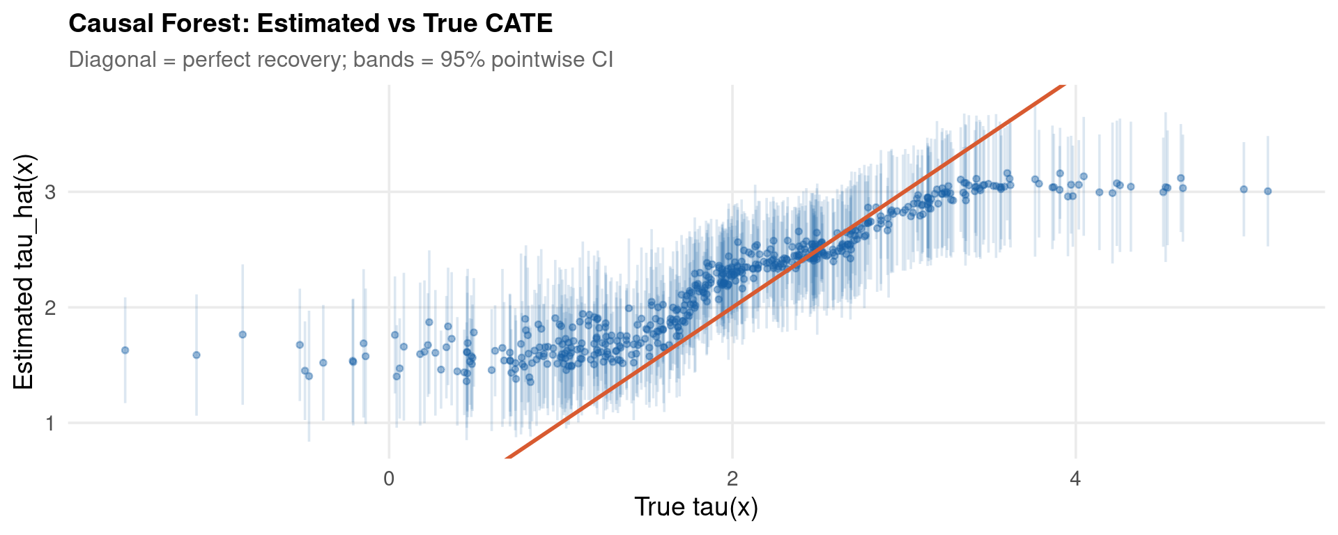
tibble(tau_true=df_cate$tau_true, tau_hat=tau_hat,
       lo=tau_hat-1.96*tau_se, hi=tau_hat+1.96*tau_se) %>%
  ggplot() +
    aes(tau_true, tau_hat) +
    geom_errorbar(aes(ymin=lo, ymax=hi), alpha=0.15, colour=col_main) +
    geom_point(alpha=0.4, size=1.2, colour=col_main) +
    geom_abline(slope=1, intercept=0, colour=col_accent, linewidth=1) +
    labs(x="True tau(x)", y="Estimated tau_hat(x)",
         title="Causal Forest: Estimated vs True CATE",
         subtitle="Diagonal = perfect recovery; bands = 95% pointwise CI") +
    theme_lecture

Causal Forest — Diagnostics

  • Leaf size (min.node.size): too small → noisy leaf effects; too large → heterogeneity averaged away
  • Honesty fraction: default 0.5; with small \(n\), honesty can leave leaves nearly empty — check honesty.prune.leaves
  • Overlap: the forest’s own \(\hat{W}(\mathbf{x})\) should stay inside \((0.05, 0.95)\)
  • Variable importance: which covariates drive the splits — sanity-check against economics
  • Calibration test (test_calibration): is the mean prediction right, and is the differential prediction informative?
Code
cat("Calibration test (DGP 2 forest):\n")
Calibration test (DGP 2 forest):
Code
print(round(unclass(test_calibration(cf)), 3))
                               Estimate Std. Error t value Pr(>t)
mean.forest.prediction            1.004      0.045  22.412      0
differential.forest.prediction    1.373      0.210   6.543      0
attr(,"method")
[1] "Best linear fit using forest predictions (on held-out data)\nas well as the mean forest prediction as regressors, along\nwith one-sided heteroskedasticity-robust (HC3) SEs"
attr(,"df")
[1] 498
attr(,"nobs")
[1] 500
attr(,"logLik")
'log Lik.' -743.6698 (df=3)
Code
vi_cf <- variable_importance(cf)
cat("\nVariable importance:\n")

Variable importance:
Code
print(setNames(round(as.numeric(vi_cf), 3), colnames(X_cf)))
   v1    v2    v3    v4    v5 
0.613 0.094 0.117 0.090 0.085 
Code
cat(sprintf("\nOverlap: %.1f%% of W_hat inside [0.05, 0.95]\n",
            100*mean(cf$W.hat > 0.05 & cf$W.hat < 0.95)))

Overlap: 100.0% of W_hat inside [0.05, 0.95]
Code
cat(sprintf("Range of W_hat: [%.3f, %.3f]\n", min(cf$W.hat), max(cf$W.hat)))
Range of W_hat: [0.274, 0.706]
  • mean.forest.prediction \(\approx 1\) with small SE → the ATE is well calibrated
  • differential.forest.prediction \(\approx 1\) and significant → the forest detects real heterogeneity; near 0 → treat the CATE map as noise
  • importance concentrating on \(v_1\) matches the DGP — in applications, an importance ranking that contradicts theory is a red flag

Application — Job Training: NSW Experiment

Data: the NSW experimental sample (LaLonde 1986; wooldridge::jtrain2), \(n = 445\) men, randomised job training. Outcome: 1978 real earnings (thousand USD).

Code
data("jtrain2", package="wooldridge")
jt_cols <- c("re78","train","age","educ","black","hisp","married","re74","re75","nodegree")

X_jt <- as.matrix(jtrain2[, jt_cols[-(1:2)]])
set.seed(14159)
cf_jt <- causal_forest(X_jt, jtrain2$re78, jtrain2$train,
                       num.trees=2000, honesty=TRUE, seed=14159)
ate_jt <- average_treatment_effect(cf_jt)
cat(sprintf("NSW training ATE: %.3f thousand USD (SE %.3f)\n",
            ate_jt["estimate"], ate_jt["std.err"]))
NSW training ATE: 1.541 thousand USD (SE 0.653)
Code
cat(sprintf("Experimental benchmark (diff in means): %.3f\n",
            mean(jtrain2$re78[jtrain2$train==1]) - mean(jtrain2$re78[jtrain2$train==0])))
Experimental benchmark (diff in means): 1.794
Code
cat("\nBest Linear Projection of tau(x):\n")

Best Linear Projection of tau(x):
Code
print(round(best_linear_projection(cf_jt, X_jt), 3))

Best linear projection of the conditional average treatment effect.
Confidence intervals are cluster- and heteroskedasticity-robust (HC3):

            Estimate Std. Error t value Pr(>|t|)
(Intercept)   -4.044      7.023  -0.576    0.565
age            0.043      0.089   0.481    0.631
educ           0.397      0.441   0.900    0.368
black          1.629      2.378   0.685    0.494
hisp           0.784      3.172   0.247    0.805
married        2.066      1.907   1.084    0.279
re74          -0.039      0.247  -0.159    0.874
re75           0.036      0.275   0.131    0.896
nodegree      -1.647      2.132  -0.773    0.440
Code
import pandas as pd, numpy as np
import wooldridge as woo
from econml.grf import CausalForest

jt = woo.data("jtrain2")[["re78","train","age","educ","black","hisp",
                          "married","re74","re75","nodegree"]]
y_jt = jt["re78"].values
W_jt = jt["train"].values
X_jt = jt.drop(columns=["re78","train"]).values

cf_jt = CausalForest(n_estimators=2000, min_samples_leaf=5,
                     honest=True, random_state=14159).fit(X_jt, W_jt, y_jt)
tau_jt = cf_jt.predict(X_jt).flatten()

q = np.percentile(tau_jt, [25, 50, 75])
out = (f"n = {len(jt)}, treated = {W_jt.sum()}\n"
       f"Mean CATE: {tau_jt.mean():.3f} thousand USD\n"
       f"Experimental benchmark: {y_jt[W_jt==1].mean()-y_jt[W_jt==0].mean():.3f}\n"
       f"CATE quartiles: Q1 {q[0]:.2f} | median {q[1]:.2f} | Q3 {q[2]:.2f}")
import sys; sys.stdout.write(out + "\n"); sys.stdout.flush()
n = 445, treated = 185
Mean CATE: 1.676 thousand USD
Experimental benchmark: 1.794
CATE quartiles: Q1 0.70 | median 1.54 | Q3 2.49
131

Meta-Learners

Any supervised learner \(\mu(\cdot)\) can estimate CATEs — the meta-strategy differs (Künzel et al. 2019):

Learner Recipe Weakness
S one model \(\mu(\mathbf{x}, W)\); \(\hat\tau = \mu(\mathbf{x},1)-\mu(\mathbf{x},0)\) regularisation can zero out \(W\)
T separate \(\mu_1, \mu_0\) per arm noisy when one arm is small
X impute \(\tilde\tau_i\) from the other arm’s model, re-fit, blend by \(\hat{e}(\mathbf{x})\) more steps, more tuning
R residualise \(y, W\) (Robinson), fit weighted \(\tilde{y}/\tilde{W}\) on \(\mathbf{x}\) needs good nuisances
Code
set.seed(14159)
y_mt <- df_cate$y; W_mt <- df_cate$W; X_mt <- as.matrix(df_cate[, paste0("v",1:5)])
i1 <- W_mt==1; i0 <- W_mt==0

# T-learner
m1 <- ranger(y~., data=data.frame(y=y_mt[i1], X_mt[i1,]), num.trees=500, seed=14159)
m0 <- ranger(y~., data=data.frame(y=y_mt[i0], X_mt[i0,]), num.trees=500, seed=14159)
tau_T <- predict(m1, data=data.frame(X_mt))$predictions -
         predict(m0, data=data.frame(X_mt))$predictions

# S-learner
mS <- ranger(y~., data=data.frame(y=y_mt, W=W_mt, X_mt), num.trees=500, seed=14159)
tau_S <- predict(mS, data=data.frame(W=1, X_mt))$predictions -
         predict(mS, data=data.frame(W=0, X_mt))$predictions

# X-learner
d1 <- y_mt[i1] - predict(m0, data=data.frame(X_mt[i1,]))$predictions
d0 <- predict(m1, data=data.frame(X_mt[i0,]))$predictions - y_mt[i0]
t1 <- ranger(y~., data=data.frame(y=d1, X_mt[i1,]), num.trees=500, seed=14159)
t0 <- ranger(y~., data=data.frame(y=d0, X_mt[i0,]), num.trees=500, seed=14159)
me <- ranger(y~., data=data.frame(y=W_mt, X_mt), num.trees=500, seed=14159)
e_hat <- pmin(pmax(predict(me, data=data.frame(X_mt))$predictions, 0.05), 0.95)
tau_X <- e_hat  * predict(t0, data=data.frame(X_mt))$predictions +
         (1-e_hat)* predict(t1, data=data.frame(X_mt))$predictions

# Causal forest benchmark (fitted earlier on the same data)
tau_CF <- predict(cf)$predictions

res_mt <- NULL
for (nm in c("T","S","X","CF")) {
  th <- get(paste0("tau_", nm))
  res_mt <- rbind(res_mt, data.frame(Learner=nm,
    RMSE=round(sqrt(mean((th-df_cate$tau_true)^2)),4),
    Cor=round(cor(th, df_cate$tau_true),3),
    `Mean tau`=round(mean(th),3), check.names=FALSE))
}
cat("Meta-learners vs causal forest (true ATE = 2.0)\n")
Meta-learners vs causal forest (true ATE = 2.0)
Code
print(res_mt, row.names=FALSE)
 Learner   RMSE   Cor Mean tau
       T 0.8779 0.669    2.319
       S 0.7701 0.678    2.099
       X 0.6018 0.839    2.173
      CF 0.6232 0.927    2.217
Code
import warnings; warnings.filterwarnings("ignore")
import numpy as np
from sklearn.ensemble import RandomForestRegressor, RandomForestClassifier
from econml.metalearners import TLearner, SLearner, XLearner

rf  = lambda: RandomForestRegressor(500, min_samples_leaf=5, random_state=14159)
rfc = lambda: RandomForestClassifier(500, min_samples_leaf=5, random_state=14159)

tl = TLearner(models=rf()).fit(Y_cf2, W_cf2, X=X_cf2)
sl = SLearner(overall_model=rf()).fit(Y_cf2, W_cf2, X=X_cf2)
xl = XLearner(models=rf(), propensity_model=rfc()).fit(Y_cf2, W_cf2, X=X_cf2)

lines = [f"{'Learner':<6} {'RMSE':>8} {'Cor':>7} {'Mean tau':>9}", "-"*34]
for nm, est in [("T", tl), ("S", sl), ("X", xl)]:
    t = est.effect(X_cf2)
    lines.append(f"{nm:<6} {np.sqrt(np.mean((t-tau_true2)**2)):>8.4f} "
                 f"{np.corrcoef(t, tau_true2)[0,1]:>7.3f} {t.mean():>9.3f}")
t = tau_hat2   # econml CausalForest from the implementation slide
lines.append(f"{'CF':<6} {np.sqrt(np.mean((t-tau_true2)**2)):>8.4f} "
             f"{np.corrcoef(t, tau_true2)[0,1]:>7.3f} {t.mean():>9.3f}")
import sys; sys.stdout.write("\n".join(lines) + "\n"); sys.stdout.flush()
Learner     RMSE     Cor  Mean tau
----------------------------------
T        0.6952   0.782     2.204
S        0.6988   0.779     2.208
X        0.5332   0.867     2.154
CF       0.5897   0.955     2.396
206

Application — Class Size: STAR with the X-Learner

Data: Tennessee STAR kindergarten cohort (Krueger 1999; AER::STAR), small classes (13–17) vs regular (22–25), randomised within schools. Outcome: reading + math score.

Code
data("STAR", package="AER")
k <- subset(STAR, !is.na(stark) & !is.na(readk) & !is.na(mathk) & stark != "regular+aide") %>%
  mutate(treat = as.integer(stark == "small"),
         score = readk + mathk)
star_df <- na.omit(data.frame(score=k$score, treat=k$treat,
  boy    = as.integer(k$gender == "male"),
  black  = as.integer(k$ethnicity == "afam"),
  lunch  = as.integer(k$lunchk == "free"),
  texp   = k$experiencek,
  tblack = as.integer(k$tethnicityk == "afam")))

set.seed(14159)
X_st <- as.matrix(star_df[, c("boy","black","lunch","texp","tblack")])
i1 <- star_df$treat==1; i0 <- star_df$treat==0
m1 <- ranger(y~., data=data.frame(y=star_df$score[i1], X_st[i1,]), num.trees=500, seed=14159)
m0 <- ranger(y~., data=data.frame(y=star_df$score[i0], X_st[i0,]), num.trees=500, seed=14159)
d1 <- star_df$score[i1] - predict(m0, data=data.frame(X_st[i1,]))$predictions
d0 <- predict(m1, data=data.frame(X_st[i0,]))$predictions - star_df$score[i0]
t1 <- ranger(y~., data=data.frame(y=d1, X_st[i1,]), num.trees=500, seed=14159)
t0 <- ranger(y~., data=data.frame(y=d0, X_st[i0,]), num.trees=500, seed=14159)
me <- ranger(y~., data=data.frame(y=star_df$treat, X_st), num.trees=500, seed=14159)
e_st <- pmin(pmax(predict(me, data=data.frame(X_st))$predictions, 0.05), 0.95)
tau_st <- e_st*predict(t0, data=data.frame(X_st))$predictions +
          (1-e_st)*predict(t1, data=data.frame(X_st))$predictions

cat(sprintf("n = %d, treated share = %.3f\n", nrow(star_df), mean(star_df$treat)))
n = 3711, treated share = 0.467
Code
cat(sprintf("Raw difference in means: %.2f points\n",
            mean(star_df$score[i1]) - mean(star_df$score[i0])))
Raw difference in means: 13.83 points
Code
cat(sprintf("X-learner ATE: %.2f points\n", mean(tau_st)))
X-learner ATE: 13.79 points
Code
cat(sprintf("CATE, free lunch:  %.2f  |  paid lunch: %.2f\n",
            mean(tau_st[star_df$lunch==1]), mean(tau_st[star_df$lunch==0])))
CATE, free lunch:  14.85  |  paid lunch: 12.83
Code
cat(sprintf("CATE, teacher exp < 5y: %.2f  |  >= 5y: %.2f\n",
            mean(tau_st[star_df$texp<5]), mean(tau_st[star_df$texp>=5])))
CATE, teacher exp < 5y: 17.41  |  >= 5y: 12.56
Code
import warnings; warnings.filterwarnings("ignore")
import pandas as pd, numpy as np
from sklearn.ensemble import RandomForestRegressor, RandomForestClassifier
from econml.metalearners import XLearner

star = pd.read_csv("../data/causal-ml-star.csv")
y_st = star["score"].values
W_st = star["treat"].values
X_st = star.drop(columns=["score","treat"]).values
lunch = star["lunch"].values
texp  = star["texp"].values

xl_st = XLearner(models=RandomForestRegressor(500, min_samples_leaf=20, random_state=14159),
                 propensity_model=RandomForestClassifier(500, min_samples_leaf=20,
                                                         random_state=14159))
xl_fitted = xl_st.fit(y_st, W_st, X=X_st)
tau_st = xl_st.effect(X_st)

out = (f"n = {len(star)}, treated share = {W_st.mean():.3f}\n"
       f"X-learner ATE: {tau_st.mean():.2f} points\n"
       f"CATE, free lunch:  {tau_st[lunch==1].mean():.2f}  |  "
       f"paid lunch: {tau_st[lunch==0].mean():.2f}\n"
       f"CATE, teacher exp < 5y: {tau_st[texp<5].mean():.2f}  |  "
       f">= 5y: {tau_st[texp>=5].mean():.2f}")
import sys; sys.stdout.write(out + "\n"); sys.stdout.flush()
n = 3711, treated share = 0.467
X-learner ATE: 13.10 points
CATE, free lunch:  15.48  |  paid lunch: 10.93
CATE, teacher exp < 5y: 17.23  |  >= 5y: 11.69
154

Uplift Modeling

Uplift = CATE used for targeting. Rank units by \(\hat\tau(\mathbf{x})\), treat from the top, and ask: does the observed treatment–control gap actually decline down the ranking?

  • if yes, the CATE model has targeting value — the marketing-science name is the uplift or Qini curve
  • a flat profile means the model ranks noise — target nobody, or everybody
  • identical mathematics to CATE validation; only the business framing differs (Gutierrez & Gérardy 2017, proceedings.mlr.press/v67)
Code
dec_pw <- ntile(-tau_pw, 10)   # decile 1 = highest predicted CATE
uplift_pw <- NULL
for (d in 1:10) {
  i <- dec_pw==d
  uplift_pw <- rbind(uplift_pw, data.frame(decile=d,
    uplift = mean(Y_pw[i & W_pw==1]) - mean(Y_pw[i & W_pw==0])))
}
data.frame(uplift_pw) %>%
  ggplot() +
    aes(factor(decile), uplift) +
    geom_col(fill=col_main, alpha=0.85) +
    geom_hline(yintercept=ate_pw["estimate"], colour=col_accent,
               linetype="dashed", linewidth=0.9) +
    labs(x="Decile of predicted CATE (1 = highest)", y="Observed uplift ($)",
         title="401(k): observed uplift by predicted-CATE decile",
         subtitle="Dashed = ATE. Declining bars = the CATE ranking has real targeting value") +
    theme_lecture

  • top deciles above the ATE line and bottom deciles below → target the top
  • policy value: treating only deciles 1–5 captures most of the total effect at half the cost
  • observed uplift per decile is itself noisy — with modest \(n\), use out-of-sample ranking (the forest’s out-of-bag \(\hat\tau\) already is)

Policy Learning

Choose an assignment rule \(\pi: \mathbf{x} \mapsto \{0, 1\}\) to maximise expected welfare (Athey & Wager 2021):

\[\max_{\pi \in \Pi} \; \mathbb{E}\big[Y(\pi(\mathbf{X}))\big] \quad\Longleftrightarrow\quad \max_{\pi \in \Pi} \; \frac{1}{n}\sum_i \hat\Gamma_i^{(\pi(\mathbf{x}_i))}\]

  • \(\hat\Gamma_i\) are doubly robust scores from the causal forest — not raw \(\hat\tau\)
  • restricting \(\Pi\) to depth-2 trees keeps the rule interpretable and auditable — essential for actual policy
  • regret bounds: the learned rule’s welfare loss vs the oracle shrinks at \(\sqrt{n}\) rates
Code
Gamma_jt <- double_robust_scores(cf_jt)
pt_jt <- policy_tree(X_jt, Gamma_jt, depth=2)
print(pt_jt)
policy_tree object 
Tree depth:  2 
Actions:  1: control 2: treated 
Variable splits: 
(1) split_variable: re74  split_value: 0.492231 
  (2) split_variable: educ  split_value: 8 
    (4) * action: 1 
    (5) * action: 2 
  (3) split_variable: re75  split_value: 8.96068 
    (6) * action: 1 
    (7) * action: 2 
Code
pol_jt <- predict(pt_jt, X_jt) - 1
gain <- mean(Gamma_jt[cbind(1:nrow(X_jt), pol_jt+1)]) - mean(Gamma_jt[,2])
cat(sprintf("\nPolicy treats %.0f%% of the sample\n", 100*mean(pol_jt)))

Policy treats 65% of the sample
Code
cat(sprintf("Estimated welfare gain vs treat-everyone: %.3f thousand USD/person\n", gain))
Estimated welfare gain vs treat-everyone: 0.618 thousand USD/person
Code
import warnings; warnings.filterwarnings("ignore")
import pandas as pd, numpy as np
import wooldridge as woo
from econml.policy import DRPolicyTree

jt2 = woo.data("jtrain2")[["re78","train","age","educ","black","hisp",
                           "married","re74","re75","nodegree"]]
y_p = jt2["re78"].values
W_p = jt2["train"].values
X_p = jt2.drop(columns=["re78","train"]).values

pt_py = DRPolicyTree(max_depth=2, min_samples_leaf=20, random_state=14159)
pt_fitted = pt_py.fit(y_p, W_p, X=X_p)
rec = pt_py.predict(X_p)

out = (f"DRPolicyTree (depth 2) treats {100*rec.mean():.0f}% of the sample\n"
       f"Feature importances: "
       + ", ".join(f"{c}={v:.2f}" for c, v in
                   zip(jt2.columns[2:], pt_py.feature_importances_) if v > 0.01))
import sys; sys.stdout.write(out + "\n"); sys.stdout.flush()
DRPolicyTree (depth 2) treats 90% of the sample
Feature importances: re74=1.00
79

Interpretability — Importance, PDP, SHAP

Interpreting a CATE model = interpreting any ML model, applied to \(\hat\tau(\mathbf{x})\):

  • Variable importance — which covariates the forest splits on
  • Partial dependence (PDP) — average \(\hat\tau\) as one covariate moves; ICE curves are per-unit PDPs and reveal interaction effects the average hides
  • SHAP values — per-observation additive decomposition of the prediction; here computed on an xgboost surrogate fitted to \(\hat\tau(\mathbf{x})\)
Code
vi_pw <- variable_importance(cf_pw)
cat("Causal forest split importance - 401(k) CATE\n")
Causal forest split importance - 401(k) CATE
Code
data.frame(Variable=colnames(X_pw), Importance=round(as.numeric(vi_pw),3)) %>%
  arrange(desc(Importance)) %>%
  print(row.names=FALSE)
 Variable Importance
      inc      0.626
      age      0.188
     educ      0.107
    fsize      0.033
     pira      0.026
     male      0.019
Code
inc_dec <- ntile(pension[[inc_col]], 10)
pdp_df <- NULL
for (d in 1:10) {
  pdp_df <- rbind(pdp_df, data.frame(decile=d,
    inc = mean(pension[[inc_col]][inc_dec==d]),
    tau = mean(tau_pw[inc_dec==d])))
}
ggplot(pdp_df) +
  aes(inc/1000, tau) +
  geom_line(colour=col_main, linewidth=1.1) +
  geom_point(colour=col_main, size=2.5) +
  geom_hline(yintercept=ate_pw["estimate"], colour=col_accent,
             linetype="dashed", linewidth=0.9) +
  labs(x="Household income (thousand $, decile means)", y="Mean estimated CATE ($)",
       title="401(k) CATE rises with income",
       subtitle="Dashed = ATE") +
  theme_lecture

Code
sur_pw <- xgb.train(list(objective="reg:squarederror", max_depth=3, eta=0.1),
                    xgb.DMatrix(X_pw, label=tau_pw), nrounds=100, verbose=0)
contrib <- predict(sur_pw, xgb.DMatrix(X_pw), predcontrib=TRUE)
shap_df <- data.frame(Variable=colnames(X_pw),
                      MeanAbsSHAP=colMeans(abs(contrib[, colnames(X_pw)])))
ggplot(shap_df) +
  aes(MeanAbsSHAP, reorder(Variable, MeanAbsSHAP)) +
  geom_col(fill=col_main, alpha=0.85) +
  labs(x="Mean |SHAP| contribution to tau_hat ($)", y=NULL,
       title="SHAP decomposition of the 401(k) CATE (xgboost surrogate)") +
  theme_lecture

Software — Heterogeneous Effects

  • grfcausal_forest(), average_treatment_effect(), best_linear_projection(), test_calibration(), double_robust_scores()
  • policytreepolicy_tree() on DR scores; depth-limited exact search
  • also in grf: instrumental forests (instrumental_forest), quantile forests — Parts IV/V
  • econml.grf.CausalForest — the grf algorithm in Python
  • econml.dml.CausalForestDML — causal forest on DML residuals
  • econml.metalearnersTLearner, SLearner, XLearner, DomainAdaptationLearner
  • econml.policyDRPolicyTree, PolicyForest
  • no native causal forest — the practical route: ddml for the residualisation, then export residuals/scores as CSV and fit the forest in R/Python
  • group ATEs by observables: interact treatment with subgroups after pdslasso/ddml
  • csdid reports group-time heterogeneity in the DiD setting — Part IV

Part IV — ML for IV, DiD & Panels

LASSO IV · ML DiD · Panel Causal Inference

Why ML for IV?

  • Many instruments: with dozens of candidate instruments, 2SLS overfits the first stage — bias toward OLS
  • Nonlinear first stages: the optimal instrument is \(\mathbb{E}[D|\mathbf{z}]\) — rarely linear in \(\mathbf{z}\)
  • Weak instruments: low first-stage signal → size distortions; adding junk instruments makes it worse
  • Selection: Lasso picks the few instruments that actually predict \(D\) (Belloni et al. 2012)
  • Flexibility: forests/boosting approximate \(\mathbb{E}[D|\mathbf{z}]\) without a functional form
  • Orthogonality carries over: the IV moment \(\mathbb{E}[\tilde{z}(\tilde{y} - \theta\tilde{D})] = 0\) with ML-residualised \(\tilde{y}, \tilde{D}, \tilde{z}\) is Neyman-orthogonal — Part II’s machinery applies
  • ML selection does not fix weak identification — if no instrument is strong, Lasso selects nothing (a feature: it tells you)
  • the exclusion restriction is still an economic assumption — no algorithm can test it
  • report the selected instruments and the first-stage fit alongside \(\hat\theta\)

LASSO IV — Theory

Sparse optimal instruments (Belloni, Chen, Chernozhukov & Hansen 2012):

\[y_i = \theta D_i + \mathbf{x}_i'\boldsymbol\beta + \varepsilon_i, \qquad D_i = f(\mathbf{z}_i, \mathbf{x}_i) + v_i\]

The efficient instrument is \(f(\mathbf{z}, \mathbf{x}) = \mathbb{E}[D|\mathbf{z}, \mathbf{x}]\); approximate it with Lasso on a large dictionary of transformations of \((\mathbf{z}, \mathbf{x})\).

  1. Lasso of \(D\) on the instrument dictionary + controls → selected instruments \(\hat{f}(\mathbf{z}, \mathbf{x})\)
  2. Lasso of \(y\) on controls and of \(D\) on controls → double-selected control set (Part II logic)
  3. 2SLS with \(\hat{f}\) as instrument and the selected controls
  4. Conventional heteroskedastic-robust inference on \(\hat\theta\)
  • \(\sqrt{n}\)-consistent and asymptotically normal under approximate sparsity
  • attains the semiparametric efficiency bound when the first stage is truly sparse
  • rigorous (plug-in) penalty level — not cross-validated — is what the theory covers (hdm, pdslasso defaults)

Application — Returns to Education: Card (1995)

Data: Card (1995), \(n = 3010\) men (NLS66), instrument: grew up near a 4-year college (nearc4). OLS is biased by ability; proximity shifts schooling cost.

Code
data("card", package="wooldridge")
card <- subset(card, !is.na(lwage))
ctrl_vars <- c("exper","expersq","black","south","smsa","smsa66",
               paste0("reg66",2:9))
ctrl_vars <- ctrl_vars[ctrl_vars %in% names(card)]

X_card <- as.matrix(card[, ctrl_vars])
y_card <- card$lwage; d_card <- card$educ

ols_card  <- lm(lwage ~ educ + exper + expersq + black + south +
                  smsa + smsa66, data=card)
tsls_card <- AER::ivreg(lwage ~ educ + exper + expersq + black + south +
                          smsa + smsa66 |
                          nearc4 + exper + expersq + black + south +
                          smsa + smsa66, data=card)

lasso_iv_card <- hdm::rlassoIV(x=X_card, d=d_card, y=y_card,
                                 z=as.matrix(card[,c("nearc4","nearc2")]))
theta_iv <- as.numeric(lasso_iv_card$coefficients[[1]])
se_iv    <- as.numeric(lasso_iv_card$se[[1]])

tibble(
  Method=c("OLS","2SLS (nearc4)","LASSO IV (PDS)"),
  Estimate=c(coef(ols_card)["educ"], coef(tsls_card)["educ"], theta_iv),
  SE=c(sqrt(vcovHC(ols_card,"HC3")["educ","educ"]),
       sqrt(vcovHC(tsls_card,"HC3")["educ","educ"]), se_iv)
) %>%
  mutate(CI=sprintf("[%.4f, %.4f]", Estimate-1.96*SE, Estimate+1.96*SE),
         across(where(is.numeric), \(x) round(x, 4))) %>%
  as.data.frame() %>%
  print(row.names=FALSE)
         Method Estimate     SE               CI
            OLS   0.0739 0.0037 [0.0667, 0.0810]
  2SLS (nearc4)   0.1188 0.0530 [0.0150, 0.2226]
 LASSO IV (PDS)   0.1289 0.0536 [0.0238, 0.2340]
Code
set.seed(14159)
X_ivf <- as.matrix(card[, c("exper","expersq","black","south","smsa","smsa66")])
ivf <- instrumental_forest(X_ivf, card$lwage, card$educ, card$nearc4,
                           num.trees=1000, seed=14159)
tau_ivf <- predict(ivf)$predictions
cat(sprintf("Instrumental forest: mean tau(x) = %.4f\n", mean(tau_ivf)))
Instrumental forest: mean tau(x) = 0.0854
Code
cat(sprintf("IQR of tau(x): [%.3f, %.3f]  (compliers respond heterogeneously)\n",
            quantile(tau_ivf, 0.25), quantile(tau_ivf, 0.75)))
IQR of tau(x): [0.012, 0.225]  (compliers respond heterogeneously)
Code
cat(sprintf("Mean tau, south = 1: %.3f  |  south = 0: %.3f\n",
            mean(tau_ivf[card$south==1]), mean(tau_ivf[card$south==0])))
Mean tau, south = 1: -0.005  |  south = 0: 0.146
Code
quietly frause card, clear
quietly drop if missing(lwage)
quietly regress lwage educ exper expersq black south smsa smsa66 reg662-reg669, robust
estimates store OLS_card
quietly ivregress 2sls lwage exper expersq black south smsa smsa66 reg662-reg669 ///
    (educ = nearc4), robust
estimates store TSLS_card
* same two raw instruments as R's rlassoIV — a richer instrument dictionary
* (e.g. nearc4 x covariate interactions) changes the complier weighting and
* therefore the LATE
quietly pdslasso lwage exper expersq black south smsa smsa66 reg662-reg669 ///
    (educ = nearc4 nearc2), robust
estimates store LASSO_IV_card
esttab OLS_card TSLS_card LASSO_IV_card, ///
    b(4) se(4) nostar keep(educ) ///
    mtitles("OLS" "2SLS" "LASSO IV") ///
    title("Card (1995): Returns to education")
Card (1995): Returns to education
---------------------------------------------------
                      (1)          (2)          (3)
                      OLS         2SLS     LASSO IV
---------------------------------------------------
educ               0.0747       0.1315       0.1315
                 (0.0036)     (0.0540)     (0.0540)
---------------------------------------------------
N                    3010         3010         3010
---------------------------------------------------
Standard errors in parentheses
Code
import pandas as pd, numpy as np
import wooldridge as woo
from sklearn.linear_model import LassoCV
from numpy.linalg import lstsq

card_py = woo.data("card")[["lwage","educ","nearc4","nearc2","exper","expersq",
                            "black","south","smsa","smsa66"]
                           + [f"reg66{i}" for i in range(2, 10)]].dropna()
reg_cols = sorted([c for c in card_py.columns if c.startswith("reg66")])
ctrl_c   = [c for c in ["exper","expersq","black","south","smsa","smsa66"]+reg_cols
            if c in card_py.columns]
X_c = card_py[ctrl_c].values
y_c = card_py["lwage"].values
d_c = card_py["educ"].values
z_c = card_py[["nearc4","nearc2"]].values

# PDS-Lasso IV — 3 steps
Xz = np.column_stack([z_c, X_c])
sel_y = LassoCV(cv=5,max_iter=5000).fit(Xz,y_c).coef_[2:] != 0
sel_d = LassoCV(cv=5,max_iter=5000).fit(Xz,d_c).coef_
sel_z = sel_d[:2] != 0; sel_x = sel_d[2:] != 0
union = sel_y | sel_x

X_sel = X_c[:, union]
z_sel = z_c[:, sel_z] if sel_z.any() else z_c[:,[0]]
# First stage
FS   = np.column_stack([z_sel, X_sel, np.ones(len(y_c))])
d_hat = FS @ lstsq(FS, d_c, rcond=None)[0]
# Second stage
SS   = np.column_stack([d_hat, X_sel, np.ones(len(y_c))])
b2   = lstsq(SS, y_c, rcond=None)[0]
ols_b = lstsq(np.column_stack([d_c,X_c,np.ones(len(y_c))]),y_c,rcond=None)[0][0]

out = (f"OLS return to educ.:      {ols_b:.4f}\n"
       f"PDS-Lasso IV return:      {b2[0]:.4f}\n"
       f"Controls selected: {union.sum()}/{len(ctrl_c)}")
import sys; sys.stdout.write(out + "\n"); sys.stdout.flush()
OLS return to educ.:      0.0747
PDS-Lasso IV return:      0.1136
Controls selected: 10/14
91

ML for GMM

The DML idea generalises to any moment model (Chernozhukov et al. 2022):

\[\mathbb{E}\big[\psi(W; \theta_0, \eta_0)\big] = 0, \qquad \partial_\eta\, \mathbb{E}\big[\psi(W; \theta_0, \eta)\big]\Big|_{\eta_0} = 0\]

  • \(\eta_0\) = conditional expectations, densities, propensities — estimated by ML with cross-fitting
  • then standard GMM: optimal weighting, over-identification tests, sandwich SEs

A non-orthogonal moment \(m(W;\theta,\eta)\) is repaired by adding its first-step influence correction \(\alpha(W)\):

\[\psi = m + \alpha, \qquad \alpha \text{ makes } \partial_\eta\,\mathbb{E}[\psi] = 0\]

  • Automatic DML: \(\alpha\) itself is learned from data (Riesz representer regression) — no manual derivation
  • partialling-out, AIPW, and the LATE score are all special cases of this construction
  • DoubleML covers PLR/IRM/IV models; econml exposes generic orthogonal moments
  • nonlinear structural GMM with ML first stages: residualise the instruments and conditional moments, keep your economic moment intact
  • weak identification and many-moments problems do not disappear — the classical GMM diagnostics still apply

ML for Panel Causal Inference

Panels bring thousands of nuisance parameters — unit and time effects:

\[y_{it} = \theta D_{it} + \alpha_i + \lambda_t + g(\mathbf{x}_{it}) + \varepsilon_{it}\]

  • fixest/reghdfe absorb \(\alpha_i, \lambda_t\) by iterated demeaning — FE are nuisance parameters, never reported
  • ML enters for \(g(\mathbf{x}_{it})\): apply DML to the within-transformed data

The panel DML recipe:

  1. Within-transform \(y\), \(D\), \(\mathbf{x}\) (or partial out FE with fixest)
  2. Cross-fit ML residualisation of \(\ddot{y}\) and \(\ddot{D}\) on \(\ddot{\mathbf{x}}\)cluster the folds by unit, never split a unit across folds
  3. Final regression of residuals; cluster-robust SEs at the unit level
  • serial correlation: observation-level cross-fitting leaks information across time within a unit — fold by unit
  • dynamics: lagged outcomes in \(\mathbf{x}\) change the estimand (sequential exogeneity) — be explicit
  • staggered treatments: TWFE with heterogeneous effects is biased — the DiD slides next

Application — Firm Productivity

Production function estimation is the original control-function problem: input choices respond to unobserved productivity \(\omega_{it}\), so OLS factor elasticities are biased. ACF (Ackerberg, Caves & Frazer 2015) recovers them with a nonparametric first stage — nuisance estimation, exactly the causal-ML pattern.

\[y_{it} = \beta_l \ell_{it} + \beta_k k_{it} + \omega_{it} + \varepsilon_{it}, \qquad \omega_{it} = h(\text{proxy}_{it}, k_{it})\]

  1. First stage: regress \(y\) nonparametrically on inputs + proxy (materials/investment) → strips \(\varepsilon\)
  2. Second stage: GMM on the Markov process of \(\omega_{it}\)\(\beta_l, \beta_k\)
  • the first stage is a pure prediction task — polynomials traditionally, any ML learner in modern practice
Code
data(chilean, package="prodest")
cat(sprintf("Chilean firms: %d obs, %d firms\n",
            nrow(chilean), length(unique(chilean$idvar))))
Chilean firms: 2544 obs, 497 firms
Code
ols_pf <- lm(Y ~ fX1 + fX2 + sX + pX, data=chilean)

set.seed(14159)
acf_pf <- prodestACF(chilean$Y, fX=cbind(chilean$fX1, chilean$fX2),
                     sX=chilean$sX, pX=chilean$pX,
                     idvar=chilean$idvar, timevar=chilean$timevar,
                     R=20, theta0=NULL)

data.frame(Method=c("OLS","ACF (control function)"),
           `Labour (blue)`=c(coef(ols_pf)["fX1"], acf_pf@Estimates$pars[1]),
           `Labour (white)`=c(coef(ols_pf)["fX2"], acf_pf@Estimates$pars[2]),
           Capital=c(coef(ols_pf)["sX"], acf_pf@Estimates$pars[3]),
           check.names=FALSE) %>%
  mutate(across(where(is.numeric), \(x) round(x, 3))) %>%
  print(row.names=FALSE)
                 Method Labour (blue) Labour (white) Capital
                    OLS         0.268          0.222   0.191
 ACF (control function)         0.155          0.159   0.137
  • ACF labour elasticities sit below OLS — OLS attributes part of unobserved productivity to labour (simultaneity bias)
  • the control function plays the role of \(\hat{g}(\mathbf{x})\) in DML: a flexible nuisance that purges endogeneity before the structural parameters are estimated
  • modern variants replace the polynomial first stage with random forests or boosting — same identification, better fit

ML for DiD

With staggered adoption and heterogeneous effects, the TWFE coefficient is a weighted average with possibly negative weights (Goodman-Bacon 2021, doi:10.1016/j.jeconom.2021.03.014) — it can even flip sign.

\[\text{TWFE} = \sum_{\text{2x2 comparisons}} w_k \,\hat\tau_k, \qquad \text{some } w_k < 0\]

Estimate clean group-time ATTs (Callaway & Sant’Anna 2021):

\[ATT(g,t) = \mathbb{E}\big[Y_t(g) - Y_t(0) \mid G = g\big]\]

each identified from group \(g\) vs not-yet/never-treated units, then aggregated (overall, dynamic/event-study, by group).

The doubly robust DiD score (Sant’Anna & Zhao 2020) needs two nuisances:

\[\hat{e}(\mathbf{x}) = \Pr(G{=}g \mid \mathbf{x}), \qquad \hat{\mu}_0(\mathbf{x}) = \mathbb{E}[\Delta y \mid \mathbf{x}, \text{comparison}]\]

  • consistent if either nuisance is right; both can be ML learners with cross-fitting
  • conditional parallel trends: covariates make the assumption more credible — ML makes the conditioning flexible

Application — Minimum Wage: ML DiD

Data: did::mpdta — 500 US counties, 2003–2007, staggered state minimum-wage increases (2004/2006/2007 cohorts). Outcome: log teen employment; control: log population.

Code
data(mpdta, package="did")

set.seed(14159)
gt <- att_gt(yname="lemp", tname="year", idname="countyreal",
             gname="first.treat", xformla=~lpop, data=mpdta,
             est_method="dr")
agg_s <- aggte(gt, type="simple")
cat(sprintf("Overall ATT (DR, never-treated control): %.4f (SE %.4f)\n",
            agg_s$overall.att, agg_s$overall.se))
Overall ATT (DR, never-treated control): -0.0418 (SE 0.0108)
Code
agg_g <- aggte(gt, type="group")
for (i in seq_along(agg_g$egt))
  cat(sprintf("  cohort %d: ATT = %.4f (SE %.4f)\n",
              agg_g$egt[i], agg_g$att.egt[i], agg_g$se.egt[i]))
  cohort 2004: ATT = -0.0846 (SE 0.0261)
  cohort 2006: ATT = -0.0202 (SE 0.0190)
  cohort 2007: ATT = -0.0288 (SE 0.0155)
Code
quietly import delimited "../data/causal-ml-mpdta.csv", clear
quietly destring _all, replace
cap rename firsttreat gvar
cap rename first_treat gvar
csdid lemp lpop, ivar(countyreal) time(year) gvar(gvar) method(dripw) agg(simple)
Difference-in-difference with Multiple Time Periods

                                                         Number of obs = 2,500
Outcome model  : least squares
Treatment model: inverse probability
------------------------------------------------------------------------------
             | Coefficient  Std. err.      z    P>|z|     [95% conf. interval]
-------------+----------------------------------------------------------------
         ATT |  -.0417518   .0115028    -3.63   0.000    -.0642969   -.0192066
------------------------------------------------------------------------------
Control: Never Treated

See Callaway and Sant'Anna (2021) for details
Code
import pandas as pd, numpy as np
from sklearn.linear_model import LogisticRegression, LinearRegression

# Hand-coded doubly robust ATT(2004, 2004), never-treated comparison
d = pd.read_csv("../data/causal-ml-mpdta.csv")
g, t, base = 2004, 2004, 2003
sub = d[d["first.treat"].isin([g, 0])]
wide = sub.pivot_table(index="countyreal", columns="year", values="lemp")
x  = sub.groupby("countyreal")["lpop"].first()
D  = (sub.groupby("countyreal")["first.treat"].first() == g).astype(int).values
dy = (wide[t] - wide[base]).values
X  = x.values.reshape(-1, 1)

ps  = LogisticRegression(C=1e6).fit(X, D).predict_proba(X)[:, 1]
mu0 = LinearRegression().fit(X[D==0], dy[D==0]).predict(X)

w1 = D / D.mean()
w0 = (1-D)*ps/(1-ps); w0 = w0/w0.mean()
att_dr = np.mean(w1*(dy-mu0)) - np.mean(w0*(dy-mu0))

out = (f"counties = {len(D)}, treated (2004 cohort) = {D.sum()}\n"
       f"Hand-coded DR ATT(2004, 2004): {att_dr:.4f}\n"
       f"(reference: R did::att_gt gives -0.0105 for this group-time)")
import sys; sys.stdout.write(out + "\n"); sys.stdout.flush()
counties = 329, treated (2004 cohort) = 20
Hand-coded DR ATT(2004, 2004): -0.0145
(reference: R did::att_gt gives -0.0105 for this group-time)
143

Synthetic ML Estimators

For aggregate units (states, regions) with a single treated unit, DiD’s parallel trends is often untenable. Synthetic methods build the counterfactual by prediction:

  • Synthetic control (Abadie): convex combination of donors matching pre-treatment path
  • Matrix completion (Athey et al. 2021, doi:10.1080/01621459.2021.1891924): treat counterfactuals as missing entries; nuclear-norm-regularised ML imputation
  • Generalised synthetic control (gsynth): interactive fixed effects \(\lambda_i' f_t\) estimated by factor models

All three are the same template: predict \(Y_{it}(0)\) for treated cells using untreated data, then

\[\hat\tau_{it} = Y_{it} - \hat{Y}_{it}(0)\]

Regularisation (weights simplex, nuclear norm, factor rank) plays exactly the role of the ML nuisance — and the same overfitting cautions apply.

  • full treatment — California Prop 99, placebo inference, matrix completion, scpi/gsynth/causaltensor — in the companion deck synthetic-control-and-matrix-completion-methods.Qmd
  • quick start: gsynth::gsynth(y ~ D, data=..., index=c("id","time"), force="two-way")

ML for Event Studies

The event-study parameter is the dynamic ATT at event time \(e = t - g\):

\[ATT^{dyn}(e) = \mathbb{E}\big[Y_{g+e}(g) - Y_{g+e}(0) \mid G = g\big] \;\text{aggregated over } g\]

  • pre-treatment (\(e < 0\)) estimates test parallel trends
  • ML residualisation of covariates makes conditional parallel trends flexible — same DR machinery per \((g,t)\) cell
  • never use a single TWFE lead/lag regression under staggered adoption — contaminated by heterogeneity (Sun & Abraham 2021)
Code
agg_d <- aggte(gt, type="dynamic")
ggdid(agg_d) +
  labs(title="Minimum wage: dynamic ATT (Callaway-Sant'Anna, DR with lpop)") +
  theme_lecture

Code
# Same real data (mpdta), second estimator: Sun-Abraham interaction-weighted
# event study - cohort-specific effects, aggregated with sample weights
es <- feols(lemp ~ sunab(first.treat, year) | countyreal + year,
            data=mpdta, cluster=~countyreal)
iplot(es, main="Minimum wage: Sun-Abraham event study (mpdta)",
      xlab="Event time (years since state minimum-wage rise)", col=col_main)

Code
att_sa <- summary(es, agg="att")
cat(sprintf("Sun-Abraham aggregated ATT: %.4f (SE %.4f)  |  CS-DiD ATT: %.4f\n",
            coef(att_sa)["ATT"], se(att_sa)["ATT"], agg_s$overall.att))
Sun-Abraham aggregated ATT: -0.0400 (SE 0.0118)  |  CS-DiD ATT: -0.0418
  • two modern staggered-DiD estimators on the same real data agree: Sun–Abraham ATT ≈ Callaway–Sant’Anna ATT ≈ −0.04 — teen employment falls about 4% after a state minimum-wage rise
  • flat pre-trends (\(e < 0\)) in the event-study plot support the (conditional) parallel-trends assumption
  • a naive TWFE lead/lag regression on these data would mix cohorts with opposite signs — the Sun–Abraham interaction weights prevent that

Software — IV, DiD & Panels

  • hdmrlassoIV(); grfinstrumental_forest()
  • didatt_gt(), aggte(), ggdid(); DRDID — the DR 2×2 building block
  • fixestfeols() high-dim FE, sunab() event studies; gsynth — generalised synthetic control
  • prodest — production functions (OP/LP/ACF)
  • econmlOrthoIV, DMLIV, DRIV for ML-IV
  • doublemlDoubleMLIIVM (LATE), DoubleMLPLIV
  • linearmodels — classical panel/IV benchmarks; pyfixest — fixest-style FE
  • CS-DiD: no mature port — hand-code the DR score (previous slide) or call R
  • ivlasso / pdslasso — sparse IV and double selection
  • csdid — Callaway–Sant’Anna with dripw (doubly robust IPW)
  • ddml — partial/IV/interactive models with ML learners
  • reghdfe — high-dimensional FE workhorse

Part V — Modern Extensions

Conformal Inference · Time-Series DML · Deep CATE · Forecasting

Conformal Inference for Causal ML

Causal-forest CIs are asymptotic and pointwise. Conformal prediction gives distribution-free, finite-sample guarantees (Lei & Candès 2021):

  1. Split: train nuisance models on one half, calibrate on the other
  2. Conformity score on calibration data: \(s_i = |Y_i - \hat\mu_{W_i}(\mathbf{x}_i)|\), per arm
  3. Band: \(\hat\tau(\mathbf{x}) \pm \big(q_{1-\alpha}^{(1)} + q_{1-\alpha}^{(0)}\big)\) with \(q\) the calibration quantiles
  • coverage holds for the individual effect \(Y(1)-Y(0)\), not just its conditional mean — hence the bands are honest about the Part III variance decomposition
  • the price: bands are wide — irreducible outcome noise is inside them
Code
data("pension", package="hdm")
df_cb <- pension %>%
  select(net_tfa, e401, age, inc, fsize, educ)
X_cb <- as.matrix(df_cb[, c("age","inc","fsize","educ")])
set.seed(14159)
tr_id <- sample(nrow(df_cb), floor(nrow(df_cb)/2))
tr <- df_cb[tr_id,]; ca <- df_cb[-tr_id,]

m1 <- ranger(y~., data=data.frame(y=tr$net_tfa[tr$e401==1], X_cb[tr_id,][tr$e401==1,]),
             num.trees=500, seed=14159)
m0 <- ranger(y~., data=data.frame(y=tr$net_tfa[tr$e401==0], X_cb[tr_id,][tr$e401==0,]),
             num.trees=500, seed=14159)
X_ca <- X_cb[-tr_id,]
mu1_ca <- predict(m1, data=data.frame(X_ca))$predictions
mu0_ca <- predict(m0, data=data.frame(X_ca))$predictions
q1 <- quantile(abs(ca$net_tfa[ca$e401==1] - mu1_ca[ca$e401==1]), 0.90)
q0 <- quantile(abs(ca$net_tfa[ca$e401==0] - mu0_ca[ca$e401==0]), 0.90)

tau_cb <- mu1_ca - mu0_ca
band   <- q1 + q0
cat(sprintf("Split-conformal 90%% band half-width: $%.0f\n", band))
Split-conformal 90% band half-width: $106309
Code
cat(sprintf("Mean T-learner CATE: $%.0f;  bands excluding 0: %.1f%%\n",
            mean(tau_cb), 100*mean(tau_cb - band > 0 | tau_cb + band < 0)))
Mean T-learner CATE: $8469;  bands excluding 0: 1.0%
Code
ord <- order(tau_cb)[seq(1, length(tau_cb), by=25)]
data.frame(rank=seq_along(ord), tau=tau_cb[ord]) %>%
  ggplot() +
    aes(rank, tau) +
    geom_ribbon(aes(ymin=tau-band, ymax=tau+band), fill=col_main, alpha=0.25) +
    geom_line(colour=col_main, linewidth=1) +
    geom_hline(yintercept=0, colour=col_accent, linetype="dashed") +
    labs(x="Units sorted by estimated CATE", y="tau_hat with conformal band ($)",
         title="401(k): split-conformal 90% bands for the individual effect",
         subtitle="Wide bands are honest: individual effects carry the full outcome noise") +
    theme_lecture

Code
import warnings; warnings.filterwarnings("ignore")
import pandas as pd, numpy as np
from sklearn.ensemble import RandomForestRegressor

df_cb = pd.read_csv("../data/causal-ml-pension.csv")
X_cb = df_cb[["age","inc","fsize","educ"]].values
y_cb = df_cb["net_tfa"].values
W_cb = df_cb["e401"].values

rng_cb = np.random.default_rng(14159)
tr_id = rng_cb.choice(len(df_cb), len(df_cb)//2, replace=False)
ca_id = np.setdiff1d(np.arange(len(df_cb)), tr_id)

rf = lambda: RandomForestRegressor(500, min_samples_leaf=5, random_state=14159)
m1 = rf().fit(X_cb[tr_id][W_cb[tr_id]==1], y_cb[tr_id][W_cb[tr_id]==1])
m0 = rf().fit(X_cb[tr_id][W_cb[tr_id]==0], y_cb[tr_id][W_cb[tr_id]==0])

X_ca, y_ca, W_ca = X_cb[ca_id], y_cb[ca_id], W_cb[ca_id]
q1 = np.quantile(np.abs(y_ca[W_ca==1] - m1.predict(X_ca[W_ca==1])), 0.90)
q0 = np.quantile(np.abs(y_ca[W_ca==0] - m0.predict(X_ca[W_ca==0])), 0.90)
tau_cb = m1.predict(X_ca) - m0.predict(X_ca)
band = q1 + q0

out = (f"Split-conformal 90% band half-width: ${band:,.0f}\n"
       f"Mean T-learner CATE: ${tau_cb.mean():,.0f};  "
       f"bands excluding 0: {100*np.mean((tau_cb-band>0)|(tau_cb+band<0)):.1f}%")
import sys; sys.stdout.write(out + "\n"); sys.stdout.flush()
Split-conformal 90% band half-width: $101,342
Mean T-learner CATE: $8,084;  bands excluding 0: 0.4%
100
  • the band covers \(Y_i(1) - Y_i(0)\), an individual quantity — compare with Part III’s CATE CIs, which cover a conditional mean
  • guarantee needs only exchangeability of the calibration sample — no asymptotics, any learner
  • refinements: conformalised quantile regression (tighter), weighted conformal for observational data (propensity-weighted exchangeability)

Orthogonal Random Forests

ORF (Oprescu, Syrgkanis & Wu 2019) pushes orthogonalisation inside the forest: every leaf runs its own locally-weighted DML — nuisances \(\hat{g}, \hat{m}\) are re-estimated locally around each target point, with forest kernel weights.

  • grf orthogonalises globally (one \(\hat{y}(\mathbf{x}), \hat{W}(\mathbf{x})\) for all splits); ORF orthogonalises locally — more robust when confounding strength varies over \(\mathbf{x}\)
  • cost: two nested estimations per prediction point — markedly slower
Code
import warnings; warnings.filterwarnings("ignore")
import pandas as pd, numpy as np
from econml.orf import DMLOrthoForest

df_orf = pd.read_csv("../data/causal-ml-pension.csv")   # real 401(k) data
rng_orf = np.random.default_rng(14159)
sub = rng_orf.choice(len(df_orf), 2000, replace=False)  # ORF is slow: subsample
d_orf = df_orf.iloc[sub]
X_orf = d_orf[["age","inc","fsize","educ"]].values      # heterogeneity drivers
W_ctl = d_orf[["marr","twoearn","db","pira","hown"]].values  # controls
T_orf = d_orf["e401"].values
Y_orf = d_orf["net_tfa"].values

orf = DMLOrthoForest(n_trees=200, min_leaf_size=50, subsample_ratio=0.5,
                     verbose=0, random_state=14159)
orf_fitted = orf.fit(Y_orf, T_orf, X=X_orf, W=W_ctl)

inc_q = np.quantile(d_orf["inc"], [0.1, 0.25, 0.5, 0.75, 0.9])
X_ev  = np.column_stack([np.full(5, np.median(d_orf["age"])), inc_q,
                         np.full(5, np.median(d_orf["fsize"])),
                         np.full(5, np.median(d_orf["educ"]))])
te_orf = orf.effect(X_ev)

lines = [f"ORF (200 trees, local DML in every leaf), n = 2000 (401(k) subsample)",
         "CATE along the income distribution (other covariates at medians):"]
for q, e in zip([10, 25, 50, 75, 90], te_orf):
    lines.append(f"  income p{q:<2d}: ${e:>8,.0f}")
import sys; sys.stdout.write("\n".join(lines) + "\n"); sys.stdout.flush()
ORF (200 trees, local DML in every leaf), n = 2000 (401(k) subsample)
CATE along the income distribution (other covariates at medians):
  income p10: $   1,190
  income p25: $   2,074
  income p50: $   3,209
  income p75: $   5,887
  income p90: $   8,424
256
  • the rising income gradient replicates the Part III causal-forest finding on the same real data — with locally re-estimated nuisances
  • strong, covariate-dependent confounding: local nuisance fits adapt where global ones average
  • large samples with mild confounding: grf/CausalForestDML deliver similar accuracy at a fraction of the cost (hence the n = 2000 subsample here)
  • panel extension — local orthogonalisation per unit-time cell — is the research frontier; the dynamic-effects slide later shows a pragmatic panel forest

Double ML for Time Series

Cross-fitting assumes exchangeable observations. Time series violate it twice:

  • random folds leak the future into the training set → use consecutive blocks as folds
  • residuals are serially correlated → the final regression needs HAC (Newey–West) standard errors

\[\hat\theta^{DML-TS}: \text{block cross-fit } \tilde{y}_t, \tilde{D}_t, \text{ then } \tilde{y}_t = \theta \tilde{D}_t + u_t, \;\; \widehat{\text{Var}}_{NW}(\hat\theta)\]

Real data: FRED-MD, 1960–2025. \(D_t = \Delta\) federal funds rate, \(y_{t+1}\) = next-month CPI inflation, \(\mathbf{X}_t\) = 120 macro series — the price puzzle in one slide.

Code
set.seed(14159)
df_ts <- read.csv("../data/causal-ml-fredmd.csv")   # created by causal-ml-data.R
y_ts  <- df_ts$y                                    # next-month inflation (ann. %)
d_ts  <- df_ts$FEDFUNDS                             # policy-rate change at t
X_ts  <- as.matrix(df_ts[, !(names(df_ts) %in% c("date","y","FEDFUNDS"))])
T_ts  <- length(y_ts)

naive_ts <- lm(y_ts ~ d_ts)
cat(sprintf("Naive OLS (no controls):  %.3f  (NW SE %.3f) - the 'price puzzle'\n",
            coef(naive_ts)["d_ts"],
            sqrt(sandwich::NeweyWest(naive_ts, lag=4)["d_ts","d_ts"])))
Naive OLS (no controls):  1.179  (NW SE 0.622) - the 'price puzzle'
Code
blocks <- cut(seq_len(T_ts), 5, labels=FALSE)   # consecutive blocks, not random folds
yr_ts <- dr_ts <- numeric(T_ts)
for (k in 1:5) {
  tr <- blocks!=k; te <- blocks==k
  fg <- ranger(y~., data=data.frame(y=y_ts[tr], X_ts[tr,]), num.trees=500, seed=14159)
  fm <- ranger(d~., data=data.frame(d=d_ts[tr], X_ts[tr,]), num.trees=500, seed=14159)
  yr_ts[te] <- y_ts[te] - predict(fg, data.frame(X_ts[te,]))$predictions
  dr_ts[te] <- d_ts[te] - predict(fm, data.frame(X_ts[te,]))$predictions
}
dml_ts <- lm(yr_ts ~ dr_ts)
se_nw  <- sqrt(sandwich::NeweyWest(dml_ts, lag=4)["dr_ts","dr_ts"])
se_hc  <- sqrt(vcovHC(dml_ts,"HC1")["dr_ts","dr_ts"])
cat(sprintf("DML (block CF): theta = %.3f\n", coef(dml_ts)["dr_ts"]))
DML (block CF): theta = 0.077
Code
cat(sprintf("  HC SE: %.3f   Newey-West SE (lag 4): %.3f\n", se_hc, se_nw))
  HC SE: 0.575   Newey-West SE (lag 4): 0.525
Code
import warnings; warnings.filterwarnings("ignore")
import pandas as pd, numpy as np
import statsmodels.api as sm
from sklearn.ensemble import RandomForestRegressor

df_ts = pd.read_csv("../data/causal-ml-fredmd.csv")   # same data as the R tab
y_ts = df_ts["y"].values
d_ts = df_ts["FEDFUNDS"].values
X_ts = df_ts.drop(columns=["date","y","FEDFUNDS"]).values
T_ts = len(y_ts)

naive = sm.OLS(y_ts, sm.add_constant(d_ts)).fit(cov_type="HAC",
                                                cov_kwds={"maxlags": 4})
blocks = np.minimum(np.arange(T_ts) * 5 // T_ts, 4)   # consecutive blocks
yr, dr = np.zeros(T_ts), np.zeros(T_ts)
for k in range(5):
    tr, te = blocks != k, blocks == k
    fg = RandomForestRegressor(n_estimators=500, max_features="sqrt",
                               random_state=14159, n_jobs=8).fit(X_ts[tr], y_ts[tr])
    fm = RandomForestRegressor(n_estimators=500, max_features="sqrt",
                               random_state=14159, n_jobs=8).fit(X_ts[tr], d_ts[tr])
    yr[te] = y_ts[te] - fg.predict(X_ts[te])
    dr[te] = d_ts[te] - fm.predict(X_ts[te])
dml_hc = sm.OLS(yr, sm.add_constant(dr)).fit(cov_type="HC1")
dml_nw = sm.OLS(yr, sm.add_constant(dr)).fit(cov_type="HAC", cov_kwds={"maxlags": 4})

out = (f"Naive OLS (no controls):  {naive.params[1]:.3f}  (NW SE {naive.bse[1]:.3f})"
       f" - the 'price puzzle'\n"
       f"DML (block CF): theta = {dml_nw.params[1]:.3f}\n"
       f"  HC SE: {dml_hc.bse[1]:.3f}   Newey-West SE (lag 4): {dml_nw.bse[1]:.3f}")
import sys; sys.stdout.write(out + "\n"); sys.stdout.flush()
Naive OLS (no controls):  1.179  (NW SE 0.624) - the 'price puzzle'
DML (block CF): theta = 0.082
  HC SE: 0.565   Newey-West SE (lag 4): 0.509
144
  • naive OLS says rate hikes raise next-month inflation — the classic price puzzle (Sims 1992): the Fed raises rates because inflation pressure is high
  • DML with 120 macro controls (random-forest nuisances, block cross-fit) makes the puzzle vanish\(\hat\theta \approx 0\), indistinguishable from zero — conditioning on the macro state removes the policy endogeneity, in the spirit of Romer & Romer (2004) with Greenbook controls
  • HC vs Newey–West: with serially correlated residuals the iid-robust SE understates uncertainty — always report HAC in time-series DML

Causal ML for Forecasting — Macro Application

Forecasting is the one task where prediction error is the criterion — the Part I dichotomy in reverse. The honest horse race, on real data: FRED-MD, forecasting next-month US CPI inflation.

FRED-MD (McCracken & Ng 2016) — the standard monthly US macro database: 121 usable series, 1960–today, maintained by the St. Louis Fed.

  • target: next-month CPI inflation (annualised %), \[y_{t+1} = 1200 \cdot \Delta \log \text{CPI}_{t+1}\]
  • predictors: all 121 series dated \(t\) (production, labour, housing, money, rates, prices), each stationarised with its McCracken–Ng transformation code
  • split: train 1960–2014, test 2015–2025 — the test window includes the COVID inflation surge
  • this is the design of Medeiros et al. (2021), whose headline finding is that random forests beat sparse linear methods for US inflation
Code
set.seed(14159)
# FRED-MD, transformed: y = next-month CPI inflation (annualised %),
# predictors = all series dated t. Created by causal-ml-data.R.
df_fm <- read.csv("../data/causal-ml-fredmd.csv")
d_fm  <- as.Date(df_fm$date)
y_fm  <- df_fm$y
X_fm  <- as.matrix(df_fm[, !(names(df_fm) %in% c("date","y"))])

Ttr   <- sum(d_fm < as.Date("2015-01-01"))   # test = 2015-2025 (incl. COVID)
Xtr_m <- X_fm[1:Ttr, ];    ytr_m <- y_fm[1:Ttr]
Xte_m <- X_fm[-(1:Ttr), ]; yte_m <- y_fm[-(1:Ttr)]
lag_i <- X_fm[, "CPIAUCSL"] * 1200           # last month's inflation

rmse_m  <- function(y, yh) sqrt(mean((y - yh)^2))
df_tr_m <- data.frame(y = ytr_m, Xtr_m)
df_te_m <- data.frame(Xte_m)
foldid  <- cut(seq_len(Ttr), 5, labels = FALSE)  # 5 contiguous time blocks

m_ar  <- lm(ytr_m ~ lag_i[1:Ttr])                # AR(1) benchmark
m_ols <- lm(y ~ ., data = df_tr_m)
m_las <- cv.glmnet(Xtr_m, ytr_m, alpha = 1, foldid = foldid)
m_rf  <- ranger(y ~ ., data = df_tr_m, num.trees = 500, min.node.size = 5,
                seed = 14159)
m_xgb <- xgb.train(list(objective = "reg:squarederror", max_depth = 3, eta = 0.05),
                   xgb.DMatrix(Xtr_m, label = ytr_m), nrounds = 300, verbose = 0)

res_fc <- data.frame(
  Method = c("AR(1)", "OLS (all p)", "Lasso", "Random Forest", "XGBoost"),
  RMSE   = c(rmse_m(yte_m, coef(m_ar)[1] + coef(m_ar)[2] * lag_i[-(1:Ttr)]),
             rmse_m(yte_m, predict(m_ols, df_te_m)),
             rmse_m(yte_m, predict(m_las, Xte_m, s = "lambda.min")),
             rmse_m(yte_m, predict(m_rf, data = df_te_m)$predictions),
             rmse_m(yte_m, predict(m_xgb, xgb.DMatrix(Xte_m)))))
res_fc <- res_fc[order(res_fc$RMSE), ]

ggplot(res_fc) +
  aes(RMSE, reorder(Method, -RMSE), fill = RMSE == min(RMSE)) +
  geom_col(alpha = 0.85, show.legend = FALSE) +
  geom_text(aes(label = sprintf("%.3f", RMSE)), hjust = -0.15, size = 3.6) +
  scale_fill_manual(values = c("TRUE" = "#1a6ea8", "FALSE" = "#999999")) +
  scale_x_continuous(expand = expansion(mult = c(0, 0.12))) +
  labs(x = "Test RMSE (annualised inflation, %)", y = NULL,
       title = sprintf("FRED-MD: 1-month-ahead US CPI inflation - winner: %s",
                       res_fc$Method[1]),
       subtitle = sprintf("T = %d months (%s to %s), p = %d, test from 2015-01",
                          length(y_fm), format(min(d_fm), "%Y-%m"),
                          format(max(d_fm), "%Y-%m"), ncol(X_fm))) +
  theme_lecture

Code
import pandas as pd, numpy as np, matplotlib.pyplot as plt
from sklearn.linear_model import LassoCV, LinearRegression
from sklearn.preprocessing import StandardScaler
from sklearn.pipeline import make_pipeline
from sklearn.ensemble import RandomForestRegressor
import xgboost as xgb
from sklearn.metrics import mean_squared_error

df_mc = pd.read_csv("../data/causal-ml-fredmd.csv")   # written by the R tab
d_mc  = pd.to_datetime(df_mc["date"])
y_mc  = df_mc["y"].values
X_mc  = df_mc.drop(columns=["date", "y"]).values
lag_i = df_mc["CPIAUCSL"].values * 1200               # last month's inflation
T_tr2 = int((d_mc < "2015-01-01").sum())
Xtr2, Xte2 = X_mc[:T_tr2], X_mc[T_tr2:]
ytr2, yte2 = y_mc[:T_tr2], y_mc[T_tr2:]
rmse = lambda a, b: mean_squared_error(a, b) ** 0.5

ar  = LinearRegression().fit(lag_i[:T_tr2].reshape(-1, 1), ytr2)
ols = LinearRegression().fit(Xtr2, ytr2)
las = make_pipeline(StandardScaler(),
                    LassoCV(cv=5, max_iter=20000)).fit(Xtr2, ytr2)
rf_ = RandomForestRegressor(500, max_features="sqrt", min_samples_leaf=5,
                            random_state=14159).fit(Xtr2, ytr2)
xm  = xgb.XGBRegressor(max_depth=3, learning_rate=0.05, n_estimators=300,
                       random_state=14159, verbosity=0).fit(Xtr2, ytr2)

methods = ["AR(1)", "OLS (all p)", "Lasso", "Random Forest", "XGBoost"]
preds   = [ar.predict(lag_i[T_tr2:].reshape(-1, 1)), ols.predict(Xte2),
           las.predict(Xte2), rf_.predict(Xte2), xm.predict(Xte2)]
rmses   = [rmse(yte2, p) for p in preds]
order   = list(np.argsort(rmses))[::-1]   # worst at bottom, winner on top

fig, ax = plt.subplots(figsize=(8, 3.4))
cols = ["#999999"] * len(order); cols[-1] = "#1a6ea8"
bars = ax.barh([methods[i] for i in order], [rmses[i] for i in order],
               color=cols, alpha=0.85)
lbls = ax.bar_label(bars, fmt="%.3f", padding=4, fontsize=9)
axopts = ax.set(
    xlabel="Test RMSE (annualised inflation, %)",
    xlim=(0, max(rmses) * 1.12),
    title=(f"FRED-MD: 1-month-ahead US CPI inflation - "
           f"winner: {methods[order[-1]]}"))
ax.grid(True, axis="x", color="#e8e8e8")
plt.tight_layout(); plt.show()

  • Random Forest wins in both implementations — replicating Medeiros et al. (2021): inflation has nonlinearities and interactions that sparse linear models miss
  • OLS with all 121 regressors overfits spectacularly — nearly twice the RMSE of the AR(1) benchmark
  • R (glmnet/ranger) and Python (sklearn) RMSEs differ in the 2nd decimal — same data, different tie-breaking inside the learners; rankings agree
  • the top three (RF, XGBoost, Lasso) are close — in practice, test equal predictive accuracy with a Diebold–Mariano test before declaring a winner

ML for Structural Causal Models

The SCM / DAG tradition (Pearl) makes identification graphical: write the causal graph, read off which adjustment sets identify the effect. ML enters twice:

  • identification stays graph-theoretic — backdoor, frontdoor, instruments are properties of the graph, not the estimator
  • estimation of the identified functional uses any ML learner — and the DML scores from Part II plug straight in
  • refutation tests (placebo treatments, random confounders, subset stability) probe the assumptions the graph encodes
Code
import warnings; warnings.filterwarnings("ignore")
import numpy as np, pandas as pd
import wooldridge as woo
from dowhy import CausalModel

# Real data: NSW job-training experiment (LaLonde 1986); experimental
# benchmark ATE = 1.794 (thousand $, 1978 earnings)
df_dw = woo.data("jtrain2")[["re78","train","age","educ","black","hisp",
                             "married","re74","re75","nodegree"]]
ctrl_dw = ["age","educ","black","hisp","married","re74","re75","nodegree"]

cm = CausalModel(data=df_dw, treatment="train", outcome="re78",
                 common_causes=ctrl_dw)
ie = cm.identify_effect(proceed_when_unidentifiable=True)
est = cm.estimate_effect(ie, method_name="backdoor.linear_regression")
plac = cm.refute_estimate(ie, est, method_name="placebo_treatment_refuter",
                          placebo_type="permute", num_simulations=10)
rand = cm.refute_estimate(ie, est, method_name="random_common_cause",
                          num_simulations=5)

out = (f"Identified estimand: backdoor via {{age, educ, race, marriage, "
       f"pre-earnings}}\n"
       f"ATE estimate: {est.value:.3f} thousand $  "
       f"(experimental benchmark: 1.794)\n"
       f"Placebo-treatment refuter: {plac.new_effect:.4f}  (should be ~0)\n"
       f"Random-common-cause refuter: {rand.new_effect:.3f}  "
       f"(should be ~{est.value:.2f})")
import sys; sys.stdout.write(out + "\n"); sys.stdout.flush()
Identified estimand: backdoor via {age, educ, race, marriage, pre-earnings}
ATE estimate: 1.676 thousand $  (experimental benchmark: 1.794)
Placebo-treatment refuter: -0.3329  (should be ~0)
Random-common-cause refuter: 1.697  (should be ~1.68)
245
  • NSW is randomised, so the backdoor estimate can be checked against the experimental benchmark of \(\$1{,}794\) — the graph-based pipeline lands close
  • the placebo refuter re-runs the analysis with a fake randomised treatment — an estimate near 0 means the pipeline does not manufacture effects
  • the random-common-cause refuter adds a synthetic confounder — the estimate should not move
  • swap backdoor.linear_regression for backdoor.econml.dml.DML to combine graph identification with DML estimation

Causal Deep Learning

Neural networks as CATE learners make sense when \(n\) is large and \(\tau(\mathbf{x})\) is a complex function of rich inputs (text, images, long histories):

  • S/T-learner with nets — the Part III recipes, MLP instead of forest
  • representation learning (TARNet/CFRNet, Shalit et al. 2017): shared covariate representation, separate heads for \(\mu_1, \mu_0\), balancing penalty
  • the Part II warning stands: at moderate \(n\), nets miss the rate condition — validate against a forest baseline
Code
import warnings; warnings.filterwarnings("ignore")
import pandas as pd, numpy as np, torch

# Real data: 401(k) eligibility (hdm::pension) - the Part III application,
# now with a deep S-learner instead of a causal forest
df_dl = pd.read_csv("../data/causal-ml-pension.csv")
feats = ["age","inc","fsize","educ","marr","twoearn","db","pira","hown"]
X_dl = df_dl[feats].values.astype(np.float32)
W_dl = df_dl["e401"].values.astype(np.float32)
Y_dl = df_dl["net_tfa"].values.astype(np.float32)

Xs = (X_dl - X_dl.mean(0)) / X_dl.std(0)
ysd = Y_dl.std()
Ys = (Y_dl - Y_dl.mean()) / ysd

gen = torch.manual_seed(14159)
XW = torch.tensor(np.column_stack([Xs, W_dl]).astype(np.float32))
Yt = torch.tensor(Ys).unsqueeze(1)
net = torch.nn.Sequential(torch.nn.Linear(XW.shape[1], 64), torch.nn.ReLU(),
                          torch.nn.Linear(64, 32), torch.nn.ReLU(),
                          torch.nn.Linear(32, 1))
opt = torch.optim.Adam(net.parameters(), lr=1e-3)
for epoch in range(300):
    opt.zero_grad()
    loss = torch.nn.functional.mse_loss(net(XW), Yt)
    loss.backward(); opt.step()

X1 = XW.clone(); X1[:, -1] = 1.0
X0 = XW.clone(); X0[:, -1] = 0.0
with torch.no_grad():
    tau_hat_dl = (net(X1) - net(X0)).squeeze().numpy() * ysd

inc_q = pd.qcut(df_dl["inc"], 4, labels=False).values
out = (f"Deep S-learner (10-64-32-1 MLP), n = {len(Y_dl)}, 401(k) eligibility\n"
       f"Estimated ATE: ${tau_hat_dl.mean():,.0f}  "
       f"(causal forest / DoubleML range: $8,900-9,400)\n"
       f"CATE by income quartile: "
       + "  ".join(f"Q{q+1}: ${tau_hat_dl[inc_q==q].mean():,.0f}" for q in range(4)))
import sys; sys.stdout.write(out + "\n"); sys.stdout.flush()
Deep S-learner (10-64-32-1 MLP), n = 9915, 401(k) eligibility
Estimated ATE: $8,829  (causal forest / DoubleML range: $8,900-9,400)
CATE by income quartile: Q1: $3,111  Q2: $5,742  Q3: $9,544  Q4: $16,921
205
  • on the real 401(k) data the net lands in the causal-forest/DoubleML ATE range and reproduces the rising income gradient from Part III — three estimator families, one answer
  • under confounding, wrap the net in the DML/DR machinery — a deep learner is a nuisance estimator, not an identification strategy
  • production tools: econml’s deep IV / DeepIV-style estimators; TARNet/CFRNet reference implementations in torch

AutoML for Causal Inference

The nuisance learner’s tuning parameters are themselves a modelling choice. The right criterion is out-of-fold nuisance fit — never the resulting \(\hat\theta\):

  • tune inside each training fold (caret, mlr3tuning, optuna) — cross-fitting already provides the honest evaluation loop
  • choosing hyper-parameters to make \(\hat\theta\) “significant” is specification search, laundered through ML
  • DoubleML + mlr3tuning and econml’s CV-wrapped learners automate this correctly
Code
set.seed(14159)
X_am <- as.matrix(df_hd[, paste0("x",1:50)])
y_am <- df_hd$y; D_am <- df_hd$D

grid_am <- expand.grid(mtry=c(7,15,25), splitrule="variance", min.node.size=c(5,20))
tuned <- caret::train(x=X_am, y=y_am, method="ranger", tuneGrid=grid_am,
                      trControl=trainControl(method="cv", number=3),
                      num.trees=300)
cat("Selected by 3-fold CV on the OUTCOME nuisance:\n")
Selected by 3-fold CV on the OUTCOME nuisance:
Code
print(tuned$bestTune)
  mtry splitrule min.node.size
6   25  variance            20
Code
dml_rf_theta <- function(mtry, min.node.size) {
  folds <- sample(rep(1:5, length.out=nrow(X_am)))
  yr <- dr <- numeric(nrow(X_am))
  for (k in 1:5) {
    tr <- folds!=k; te <- folds==k
    fg <- ranger(y~., data=data.frame(y=y_am[tr], X_am[tr,]), num.trees=300,
                 mtry=mtry, min.node.size=min.node.size, seed=14159)
    fm <- ranger(D~., data=data.frame(D=D_am[tr], X_am[tr,]), num.trees=300,
                 mtry=mtry, min.node.size=min.node.size, seed=14159)
    yr[te] <- y_am[te] - predict(fg, data=data.frame(X_am[te,]))$predictions
    dr[te] <- D_am[te] - predict(fm, data=data.frame(X_am[te,]))$predictions
  }
  fit <- lm(yr ~ dr)
  c(unname(coef(fit)["dr"]), sqrt(vcovHC(fit,"HC3")["dr","dr"]))
}
set.seed(14159)
def_res <- dml_rf_theta(mtry=floor(sqrt(50)), min.node.size=5)
tun_res <- dml_rf_theta(tuned$bestTune$mtry, tuned$bestTune$min.node.size)
cat(sprintf("\nDML-RF, default RF:  theta = %.4f (SE %.4f)\n", def_res[1], def_res[2]))

DML-RF, default RF:  theta = 2.4658 (SE 0.0741)
Code
cat(sprintf("DML-RF, tuned RF:    theta = %.4f (SE %.4f)   (true = 2.0)\n",
            tun_res[1], tun_res[2]))
DML-RF, tuned RF:    theta = 2.2069 (SE 0.0625)   (true = 2.0)
Code
import warnings; warnings.filterwarnings("ignore")
import pandas as pd, numpy as np
from sklearn.ensemble import RandomForestRegressor
from sklearn.model_selection import GridSearchCV, KFold

df_am = pd.read_csv("../data/causal-ml-dgp1.csv")    # same DGP-1 data as the R tab
y_am = df_am["y"].values
D_am = df_am["D"].values
X_am = df_am.drop(columns=["y","D"]).values
n_am = len(y_am)

grid = {"max_features": [7, 15, 25], "min_samples_leaf": [5, 20]}
gs = GridSearchCV(RandomForestRegressor(300, random_state=14159), grid, cv=3)
gs_fitted = gs.fit(X_am, y_am)

def dml_rf(params):
    yr, dr = np.zeros(n_am), np.zeros(n_am)
    for tr, te in KFold(5, shuffle=True, random_state=14159).split(X_am):
        fg = RandomForestRegressor(300, random_state=14159, **params).fit(X_am[tr], y_am[tr])
        fm = RandomForestRegressor(300, random_state=14159, **params).fit(X_am[tr], D_am[tr])
        yr[te] = y_am[te] - fg.predict(X_am[te])
        dr[te] = D_am[te] - fm.predict(X_am[te])
    th = np.dot(dr, yr)/np.dot(dr, dr)
    psi = dr*(yr - th*dr)
    return th, ((dr**2).mean()**(-2)*(psi**2).mean()/n_am)**0.5

th_d, se_d = dml_rf({"max_features": "sqrt", "min_samples_leaf": 5})
th_t, se_t = dml_rf(gs.best_params_)
out = (f"Selected by 3-fold CV on the OUTCOME nuisance: {gs.best_params_}\n"
       f"DML-RF, default RF:  theta = {th_d:.4f} (SE {se_d:.4f})\n"
       f"DML-RF, tuned RF:    theta = {th_t:.4f} (SE {se_t:.4f})   (true = 2.0)")
import sys; sys.stdout.write(out + "\n"); sys.stdout.flush()
Selected by 3-fold CV on the OUTCOME nuisance: {'max_features': 25, 'min_samples_leaf': 5}
DML-RF, default RF:  theta = 2.5200 (SE 0.0731)
DML-RF, tuned RF:    theta = 2.2311 (SE 0.0626)   (true = 2.0)
202

ML for Missing Data

Missing covariates interact with causal ML in two ways:

  • complete-case analysis discards information and, when missingness relates to \(\mathbf{x}\), tilts the sample
  • ML imputation (missForest: iterative random-forest imputation, Stekhoven & Bühlmann 2012) preserves nonlinear relations among covariates
  • impute covariates only — never the outcome or the treatment; and remember imputation assumes MAR
Code
set.seed(14159)
data("pension", package="hdm")
df_ms <- pension[sample(9915, 2500),
           c("net_tfa","e401","age","inc","fsize","educ","marr","pira","hown")]

po_lasso <- function(dat) {
  X <- as.matrix(dat[, setdiff(names(dat), c("net_tfa","e401"))])
  e <- hdm::rlassoEffect(x=X, y=dat$net_tfa, d=dat$e401, method="partialling out")
  c(e$alpha, e$se)
}
full_ms <- po_lasso(df_ms)

df_hole <- df_ms %>%
  mutate(inc = replace(inc, sample(n(), 500), NA),   # 20% MCAR holes
         age = replace(age, sample(n(), 500), NA))
cc_ms <- po_lasso(na.omit(df_hole))

imp_ms <- missForest(df_hole[, c("age","inc","fsize","educ","marr","pira","hown")])
df_imp <- cbind(df_hole[, c("net_tfa","e401")], imp_ms$ximp)
mf_ms  <- po_lasso(df_imp)

data.frame(Sample=c("Full data (benchmark)","Complete cases (n varies)","missForest-imputed"),
           n=c(nrow(df_ms), nrow(na.omit(df_hole)), nrow(df_imp)),
           `e401 effect`=sprintf("$%.0f", c(full_ms[1], cc_ms[1], mf_ms[1])),
           SE=sprintf("$%.0f", c(full_ms[2], cc_ms[2], mf_ms[2])),
           check.names=FALSE) %>%
  print(row.names=FALSE)
                    Sample    n e401 effect    SE
     Full data (benchmark) 2500      $-1871 $2872
 Complete cases (n varies) 1595       $-684 $3328
        missForest-imputed 2500       $-869 $2861
Code
import warnings; warnings.filterwarnings("ignore")
import pandas as pd, numpy as np
import statsmodels.api as sm
from sklearn.experimental import enable_iterative_imputer
from sklearn.impute import IterativeImputer
from sklearn.ensemble import RandomForestRegressor
from sklearn.linear_model import LassoCV

rng_ms = np.random.default_rng(14159)
df_ms = pd.read_csv("../data/causal-ml-pension.csv")
df_ms = df_ms.iloc[rng_ms.choice(len(df_ms), 2500, replace=False)][
    ["net_tfa","e401","age","inc","fsize","educ","marr","pira","hown"]].reset_index(drop=True)

def po_lasso(dat):
    X = dat.drop(columns=["net_tfa","e401"]).values
    sd = X.std(axis=0); Xs = (X - X.mean(axis=0)) / sd
    yr = dat["net_tfa"].values - LassoCV(cv=5, max_iter=10000,
            random_state=14159).fit(Xs, dat["net_tfa"]).predict(Xs)
    dr = dat["e401"].values - LassoCV(cv=5, max_iter=10000,
            random_state=14159).fit(Xs, dat["e401"]).predict(Xs)
    f = sm.OLS(yr, sm.add_constant(dr)).fit(cov_type="HC1")
    return f.params[1], f.bse[1]

full_b, full_se = po_lasso(df_ms)
df_hole = df_ms.copy()
df_hole.loc[rng_ms.choice(2500, 500, replace=False), "inc"] = np.nan
df_hole.loc[rng_ms.choice(2500, 500, replace=False), "age"] = np.nan
cc = df_hole.dropna()
cc_b, cc_se = po_lasso(cc)

covs = ["age","inc","fsize","educ","marr","pira","hown"]
imp = IterativeImputer(estimator=RandomForestRegressor(50, n_jobs=-1,
        random_state=14159), max_iter=5, random_state=14159)
df_imp = df_hole.copy(); df_imp[covs] = imp.fit_transform(df_hole[covs])
mf_b, mf_se = po_lasso(df_imp)

lines = [f"{'Sample':<28} {'n':>5} {'e401 effect':>12} {'SE':>8}", "-"*57,
         f"{'Full data (benchmark)':<28} {len(df_ms):>5} {full_b:>12,.0f} {full_se:>8,.0f}",
         f"{'Complete cases':<28} {len(cc):>5} {cc_b:>12,.0f} {cc_se:>8,.0f}",
         f"{'RF-IterativeImputer':<28} {len(df_imp):>5} {mf_b:>12,.0f} {mf_se:>8,.0f}"]
import sys; sys.stdout.write("\n".join(lines) + "\n"); sys.stdout.flush()
Sample                           n  e401 effect       SE
---------------------------------------------------------
Full data (benchmark)         2500        6,099    2,461
Complete cases                1592        3,000    3,605
RF-IterativeImputer           2500        8,206    2,441
286

ML for Mediation Analysis

Split a total effect into the part flowing through a mediator \(M\) and the direct remainder:

\[\text{total} = \underbrace{\mathbb{E}[Y(1, M(1)) - Y(0, M(1))]}_{\text{direct}} + \underbrace{\mathbb{E}[Y(0, M(1)) - Y(0, M(0))]}_{\text{indirect}}\]

Identification needs sequential ignorability — treatment and mediator unconfounded given \(\mathbf{x}\). The efficient scores involve four nuisance functions; causalweight::medDML (Farbmacher et al. 2022) estimates them all by ML with cross-fitting.

R only on this slide: neither Python nor Stata has a mature DML-mediation implementation — medDML is the reference.

Code
# Real data: Job Corps experiment (causalweight::JC, n = 9,240).
# D = random assignment to Job Corps, M = share of weeks employed in year 2,
# Y = weekly earnings in year 4 ($). Schochet et al. (2008) benchmark: ~$20/week.
data("JC", package = "causalweight")
set.seed(14159)
x_jc <- JC[, 2:28]           # baseline covariates (pre-assignment)

med <- causalweight::medDML(y = JC$earny4, d = JC$assignment,
                            m = JC$pworky2, x = x_jc, k = 3)
res_md <- med$results
cat(sprintf("Job Corps -> year-4 weekly earnings, mediator: year-2 employment (n=%d)\n",
            nrow(JC)))
Job Corps -> year-4 weekly earnings, mediator: year-2 employment (n=9240)
Code
data.frame(Effect=c("Total","Direct (treated)","Indirect (treated)"),
           Estimate=round(res_md["effect", c("total","dir.treat","indir.treat")], 3),
           SE=round(res_md["se", c("total","dir.treat","indir.treat")], 3),
           p=round(res_md["p-val", c("total","dir.treat","indir.treat")], 4)) %>%
  print(row.names=FALSE)
             Effect Estimate    SE      p
              Total   19.113 3.938 0.0000
   Direct (treated)   20.799 3.793 0.0000
 Indirect (treated)   -2.477 1.173 0.0348
  • the total effect ≈ $+19/week matches the experimental Job Corps literature (Schochet, Burghardt & McConnell 2008)
  • the indirect channel is negative: Job Corps reduces year-2 employment (lock-in — participants are still in training), which transmits negatively to year-4 earnings
  • the direct (human-capital) effect more than offsets the lock-in — exactly the decomposition a plain ATE hides

ML for Dynamic Treatment Effects

Effects that evolve with time since treatment and vary across units at once — the intersection of Part III (CATE) and Part IV (event studies):

  • target: \(\tau(\mathbf{x}, e) = \mathbb{E}[Y_{g+e}(g) - Y_{g+e}(0) \mid \mathbf{X} = \mathbf{x}]\)
  • pragmatic estimator: causal forest on within-demeaned panel data with event time in the covariates
  • frontier: per-period DR scores + forest aggregation; sequential treatments need \(g\)-computation / dynamic DML
Code
set.seed(14159)
N_dy <- 300L; T_dy <- 8L
pan <- expand.grid(id=1:N_dy, t=1:T_dy)
x_i  <- rnorm(N_dy); a_i <- rnorm(N_dy)
g_i  <- sample(c(4L, 6L, 100L), N_dy, replace=TRUE)   # adopt at t=4, 6, or never
pan <- pan %>%
  mutate(x = x_i[id], g = g_i[id],
         W = as.integer(t >= g),
         e = ifelse(W == 1, t - g, -1),
         tau = (1 + 0.5*x + 0.4*e) * W,
         y = a_i[id] + 0.2*t + tau + rnorm(n(), 0, 0.5))

pan <- pan %>% group_by(id) %>% mutate(y_dm = y - mean(y)) %>%
  group_by(t) %>% mutate(y_dm = y_dm - mean(y_dm)) %>% ungroup()

X_dy <- as.matrix(pan[, c("x","t")])
set.seed(14159)
cf_dy <- causal_forest(X_dy, pan$y_dm, pan$W, num.trees=1000, seed=14159)
tau_dy <- predict(cf_dy)$predictions

res_dy <- NULL
for (ev in 0:3) {
  i <- pan$W==1 & pan$e==ev
  res_dy <- rbind(res_dy, data.frame(`Event time`=ev,
    `True mean tau`=round(mean(pan$tau[i]), 3),
    `CF estimate`=round(mean(tau_dy[i]), 3), check.names=FALSE))
}
cat("Panel causal forest: dynamic CATE by event time\n")
Panel causal forest: dynamic CATE by event time
Code
print(res_dy, row.names=FALSE)
 Event time True mean tau CF estimate
          0         0.982       0.432
          1         1.382       0.677
          2         1.782       1.025
          3         2.217       0.824
Code
import warnings; warnings.filterwarnings("ignore")
import pandas as pd, numpy as np
from econml.grf import CausalForest

pan = pd.read_csv("../data/causal-ml-dynpanel.csv")   # same panel as the R tab
pan["y_dm"] = pan["y"] - pan.groupby("id")["y"].transform("mean")
pan["y_dm"] = pan["y_dm"] - pan.groupby("t")["y_dm"].transform("mean")

X_dy = pan[["x","t"]].values
cf_dy = CausalForest(n_estimators=1000, min_samples_leaf=5, honest=True,
                     random_state=14159).fit(X_dy, pan["W"].values, pan["y_dm"].values)
tau_dy = cf_dy.predict(X_dy).flatten()

lines = [f"{'Event time':>10} {'True mean tau':>14} {'CF estimate':>12}", "-"*38]
for ev in range(4):
    i = (pan["W"]==1) & (pan["e"]==ev)
    lines.append(f"{ev:>10} {(1+0.5*pan['x'][i]+0.4*pan['e'][i]).mean():>14.3f} "
                 f"{tau_dy[i].mean():>12.3f}")
import sys; sys.stdout.write("\n".join(lines) + "\n"); sys.stdout.flush()
Event time  True mean tau  CF estimate
--------------------------------------
         0          0.982        0.410
         1          1.382        0.666
         2          1.782        0.967
         3          2.217        0.883
234

Software — Modern Extensions

  • grf — forests everywhere; policytree; conformal bands hand-coded in ~20 lines
  • causalweightmedDML() mediation; missForest — RF imputation
  • caret / mlr3tuning — nuisance hyper-parameter tuning inside folds
  • sandwich::NeweyWest() — HAC for time-series DML
  • econml.orf.DMLOrthoForest — local orthogonalisation; econml.dml.CausalForestDML
  • dowhy — graph identification + refutation tests, econml back-ends
  • torch — deep CATE / representation learning (TARNet-style)
  • optuna (ships with doubleml) — hyper-parameter search
  • time-series DML: ddml residualisation + newey on the residual regression
  • mediation: paramed / custom potential-outcome code; conformal & forests: export to R/Python
  • the honest summary: Part V topics are where Stata hands over to R/Python

Exercises — Estimation

  1. Nuisance learner robustness: replace the Lasso nuisance in the union-premium application (Part II) with random forest and gradient boosting. Does the point estimate move? Does the standard error? Report all three side by side.

  2. Cross-fitting folds: re-run the 401(k) DML estimate with \(K \in \{2, 5, 10, 20\}\) folds, holding the learner fixed. Plot \(\hat\theta\) and its SE against \(K\). Where does the estimate stabilise, and what does that cost in run time?

  3. Causal Forest BLP: on the 401(k) data, run best_linear_projection() against income, age and education. Is income the dominant driver of heterogeneity, or does it only look that way because it is correlated with eligibility?

  4. LASSO IV weak instruments: reduce the first-stage signal gradually in the Card (1995) application. At what concentration parameter does Lasso stop selecting the instruments altogether, and what happens to the 2SLS point estimate just before it does?

  5. Staggered DML: treat union entry as staggered in wagepan. Compare DML-Lasso with the two-way fixed-effects estimator, then with the Callaway–Sant’Anna ATT(g,t). Which two agree, and why?

  6. Meta-learner comparison: on the STAR data, estimate the CATE with the S-, T-, and X-learner using the same base learner. Where do they diverge most — in the tails of the covariate distribution, or the middle?

Exercises — Testing

  1. DML coverage simulation: with \(\theta_0 = 2\), \(n = 300\), \(p = 40\), run 500 Monte Carlo replications of DML-Lasso (5-fold cross-fitting) against the naive plug-in estimator. Report empirical coverage of the nominal 95% CI for each. Which one is honest?

  2. Orthogonality check: verify numerically that the DML score satisfies the Neyman orthogonality condition — perturb the fitted nuisance functions by a small \(\delta\) and confirm the estimating equation’s derivative vanishes. Repeat for the naive plug-in score and show that it does not.

  3. Omnibus heterogeneity test: run test_calibration() on the 401(k) causal forest. Does the deck’s forest pass the mean-prediction and differential-prediction tests? If it fails one, which, and what does that failure imply for the policy tree built on those scores?

  4. Placebo refutation: use the dowhy placebo-treatment refuter on the union-premium estimate. The refuted effect should be indistinguishable from zero — is it? Now repeat with a random-common-cause refuter and interpret any drift.

  5. Conformal coverage: construct conformalised prediction intervals for the individual treatment effect (Part V) and check empirical coverage on a held-out fold at nominal 90%. Does coverage hold marginally, and does it still hold conditionally within income quartiles?

  6. Propensity trimming sensitivity: re-estimate the 401(k) ATE trimming propensity scores at \(\{0, 0.01, 0.05, 0.10\}\). Plot \(\hat\theta\) against the trimming threshold. How much of the reported effect is driven by units near the overlap boundary?

References and Further Reading

Double/Debiased Machine Learning

Causal Forest and Heterogeneous Treatment Effects

LASSO IV and Post-Double-Selection

  • Belloni, Chernozhukov & Hansen (2012). Sparse models and methods for optimal instruments. doi:10.1093/restud/rds044
  • Belloni, Chernozhukov & Hansen (2014). Inference on treatment effects after selection among high-dimensional controls. doi:10.1093/restud/rdt044
  • Belloni, Chernozhukov & Hansen (2014). High-dimensional methods in economics. doi:10.1257/jep.28.2.29
  • Chernozhukov, Hansen & Spindler (2015). Post-selection and post-regularization inference (partialling-out). doi:10.1257/aer.p20151022
  • Card (1995). Using geographic variation in college proximity to estimate the return to schooling. doi:10.3386/w4483

Econometric perspectives

  • Athey & Imbens (2019). Machine learning methods that economists should know about. doi:10.1146/annurev-economics-080217-053433
  • Abadie (2003). Semiparametric instrumental variable estimation of treatment response models. doi:10.1016/S0304-4076(02)00201-4
  • Hansen (2022). Econometrics. Princeton University Press — Ch. 29 (Machine Learning), §29.20–29.22 (double-selection, partialling-out, DML)

Lecture notes and books (free)

  • Chernozhukov et al. Applied Causal Inference Powered by ML and AI. causalml-book.org
  • Huntington-Klein (2022). The Effect: An Introduction to Research Design and Causality. theeffectbook.net

Software

Thank You

Athanassios Stavrakoudis
Applied Informatics and Computational Economics Lab
Department of Economics
University of Ioannina, Greece

astavrak@uoi.gr · linkedin.com/in/astavrakoudis