Part I — The Gravity Equation the fact, the Armington foundation, multilateral resistance, zeros
Part II — A Known-Truth Laboratory simulate a world, then see which estimator finds it again
Part III — Structural Gravity in Practice three-way fixed effects, domestic flows, trade agreements
Part IV — Estimator Choice the PML family, RESET, separation
Part V — The Trade Elasticity Head–Ries, tetrads, Caliendo–Parro
Part VI — General Equilibrium exact hat algebra, the fixed point, gains from trade
Part VII — Multi-Sector & Input–Output Caliendo–Parro with linkages, calibrated on FIGARO
Part VIII — Global Value Chains Leontief inverse, value-added exports, upstreamness
Part IX — Firm Heterogeneity & Practice Melitz, margins, exercises, further reading
Three deliberate departures from the standard order used in this lecture series. All three are choices, not drift.
1. The required sequence runs once, across the front matter and Parts I–II. Packages → Problem → Methodology → DGP → Diagnostics → Estimation → Results Table is delivered there in full. Each later part then re-enters at The Problem & the Data and closes with Summary: Routines & Practice. Nine parts cannot each carry the whole sequence without burying the content.
2. The literature is reviewed once, at the end. There is no front-matter survey slide; Further Reading in Part IX carries the whole bibliography, opening with the four references that cover the entire deck. A reading list is more useful after the methods than before them, and stating the same papers twice cost a slide that How the Data Got Here now uses.
3. The tests are distributed, not collected. RESET and the separation check sit in Part IV beside the estimator they judge; the solver’s validation-against-truth sits in Part VI beside the solver. Each still gets its own theory slide and its own code slide.
This deck is about modelling trade flows and then asking what they would be under a different policy.
Three companion decks own neighbouring ground and are not repeated here:
Networks and Trade Analysis — graphs, centrality, communities, the EU trade network. That deck asks who is connected to whom; this one asks what those flows would be under a different trade policy.
Structural Estimation in Econometrics — GMM, SMM, BLP demand, dynamic discrete choice. Gravity here is estimated by pseudo-maximum likelihood, and the general-equilibrium model is solved, not GMM-estimated.
Bootstrap Methods in Econometrics — resampling theory. Part III uses the pair cluster bootstrap but does not re-derive it.
Most slides carry three tabs — R, Python, Stata. Some carry two.
Where Stata has no route to the method at all, the Stata tab is simply absent rather than present-and-apologetic. The Software Toolkit slide at the end lists exactly which methods those are and why.
Required Packages
library(fixest) # feols(), fepois() — PPML with high-dimensional FElibrary(data.table) # fread() on piped/filtered multi-GB source fileslibrary(nleqslv) # Broyden solver for the GE fixed pointlibrary(Matrix) # sparse ICIO algebra, solve() for the Leontief inverselibrary(countrycode) # ISO3 <-> country name <-> region aggregationlibrary(sandwich) # vcovCL() — clustered and two-way clustered variancelibrary(lmtest) # coeftest() — RESET and coefficient testslibrary(modelsummary) # msummary() — the results tables and their LaTeXlibrary(tidyverse) # data wrangling & ggplot2library(patchwork) # multi-panel figureslibrary(ggrepel) # non-overlapping country labelslibrary(png) # readPNG() — reload Stata-exported graphs
import numpy as np # arrays, linear algebra, Leontief inverseimport pandas as pd # data frames, CSV inputimport pyfixest as pf # pf.fepois() — PPML with multiple FEimport statsmodels.api as sm # GLM/Poisson, RESET, robust covariancefrom scipy.optimize import root # the GE fixed pointfrom scipy import stats # distributions, Pareto tail fittingimport matplotlib.pyplot as plt # all figures
* SSC packagesssc install ppmlhdfe // PPML with high-dimensional fixed effectsssc install ppml // Santos Silva-Tenreyro's originalssc install ppml_panel_sg // structural gravity with exporter/importer-time FEssc install reghdfe // linear analogue, used for the log-OLS benchmarksssc install ftools // reghdfe/ppmlhdfe dependencyssc install estout // esttab — the results tables* Shipped with Stata SEpoisson, glm// the PML family: Poisson, Gamma, Gaussianestatovtest// RESETmata// Leontief inverse and the GE fixed point
The matrix work — the Leontief inverse in Part VIII and the fixed-point iteration in Parts VI and VII — runs in Mata, which has no matsize ceiling. The aggregated input–output system is deliberately kept at \(96 \times 96\) so all three languages invert it comfortably.
50 countries, 4 broad sectors, 2000–2016, with domestic flows
46 523
ctm-sim.csv · ctm-sim-truth.csv
Simulated Armington world, seed 14159
60 countries, known \(\theta\), known counterfactual
3 600 · 60
ctm-icio.csv
Eurostat FIGARO
12 regions × 8 sectors, 2022
10 464
ctm-firms.csv
Eurostat TEC
32 countries, size classes and top-\(k\) shares, 2015–2024
15 586
ctm-tariffs.csv
WITS/TRAINS applied MFN rates, 2020
EU–US tariffs by sector, for the Part VII counterfactual
60
On every slide that follows, R, Python and Stata read the same file. Any disagreement between the three tabs is therefore a real disagreement between methods, never a difference in the data.
The datasets most trade courses still use stopped a decade or more ago: the WTO Advanced Guide panel ends in 2006, the gravity package ships a 2006 cross-section, and WIOD’s last table is 2014.
Every source above is the current release, running to 2020, 2019 and 2024 respectively. The methods are the same; the world they describe is not.
Two of the covariates are genuinely new and get a slide of their own in Part III: scaled_sci_2021, Facebook’s Social Connectedness Index between country pairs, and diplo_disagreement, distance in United Nations voting records.
ctm-itpde.csv keeps the rows where exporter equals importer — a country’s trade with itself.
Almost every classroom gravity dataset throws those away. Without them the multilateral resistance terms are not identified from trade data alone, the border effect cannot be measured at all, and the trade elasticity has to be imported from someone else’s paper. Parts III, V and VI all rest on that diagonal.
The price is real and worth stating: ITPD-E builds domestic flows only where the production statistics allow it, so China, Switzerland, Malaysia and Thailand are not in the 50-country sample. Manufacturing is complete for all 50 countries in all five waves; services and mining have gaps.
CEPII Gravity V202211 arrives as a 207 MB zip holding one CSV member of roughly 1.3 GB and 87 columns. Reading it whole costs several GB of memory to build a table we then discard 95% of.
ITPD-E Release 3 is a 982 MB zip carrying 170 industries. The deck uses four broad sectors.
Neither file is downloaded, unpacked and then filtered. Both are filtered while being read, so nothing bigger than the surviving rows is ever in memory. Three ordinary tools do all of it — unzip -p, funzip, gawk — and they turn any oversized public archive into a table that fits.
The two recipes on the next tabs are the ones that fetched these files, and they transfer: point either at another oversized public archive and it downloads once, filters during the read, and lands a table you can actually open.
data.table::fread takes a shell command in place of a filename. The pipe runs, gawk keeps the six waves, and only those rows are ever parsed by R.
unzip -p writes the member to stdout, so the 1.3 GB CSV never touches disk.
select = drops 57 of the 87 columns before they reach R.
The file.exists guard makes the script re-runnable: raw downloads are cached in ../data/, and a second run costs seconds instead of 300 MB.
ITPD-E is never unzipped at all. funzip inflates the stream as it arrives, gawk sums 170 industries into 4 broad sectors on the fly, and what reaches the disk is the finished 17 MB aggregate.
The trap that costs an afternoon. ITPD-E’s industry and country names are quoted and contain commas, so -F, misaligns every field after the sixth — silently, with no error, producing a table of plausible nonsense. patsplit() with the pattern ([^,]*)|("[^"]*") respects the quotes.
Note the two-stage parse: the year filter runs on $3 under plain FS=",", which is safe because fields 1–3 all precede the first quoted field. Cheap test first, expensive correct split only on the rows that survive.
Two source archives of about 1.3 GB and 982 MB, plus two Eurostat downloads and two WITS queries, reduce to the few MB above. The counts are read off the files themselves, so this table cannot go stale if a vintage changes — it will simply report different numbers, which is the point.
The access patterns are the providers’ own, not inventions of this deck:
Conte, Cotterlaz & Mayer (2022), The CEPII Gravity Database, CEPII WP 2022-05 — column dictionary and usage notes. cepii.fr
Borchert, Larch, Shikher & Yotov (2021), The International Trade and Production Database for Estimation, International Economics 166 — construction, and why the domestic diagonal exists. 10.1016/j.inteco.2020.08.001
Eurostat, FIGARO inter-country supply, use and input–output tables — methodology and the naio_10_fcp_ii4 bulk endpoint. ec.europa.eu/eurostat
The answer that has survived sixty years of testing is that trade rises with economic size and falls with distance:
\[
X_{ij} \;=\; G \cdot \frac{Y_i^{\alpha}\, Y_j^{\beta}}{D_{ij}^{\delta}}
\]
Tinbergen wrote that down in 1962 by analogy with Newton, fitted it, and found it worked. It kept working for twenty years before anyone could say why.
That gap matters. An equation that fits but has no structure cannot answer the question we actually care about — what happens to trade if policy changes? The rest of Part I closes the gap, and then breaks the naive estimator that everybody starts with.
../data/ctm-gravity.csv — CEPII Gravity V202211.
150 largest traders, six waves: 2000, 2004, 2008, 2012, 2016, 2020
133 206 rows, of which 132 306 are international pairs
goods exports from BACI, in thousand USD
distance, contiguity, common language, colonial history, religion
GDP, population, GDP per capita, WTO and EU membership, trade agreements
and two covariates that did not exist a decade ago — the Facebook Social Connectedness Index and distance in United Nations voting records
Four-year waves rather than annual data: trade costs take time to adjust, and consecutive years of a gravity panel are far from independent observations.
Look at the fact itself, on one scatter plot
Derive it from consumer demand, so it has structure
Discover that structure implies a term nobody can observe
Estimate the naive log-linear regression everybody starts with
Notice that it silently discarded a tenth of the data
Notice that what it did keep, it got wrong
Steps 5 and 6 are the argument for everything in Parts II to IV.
The Gravity Fact
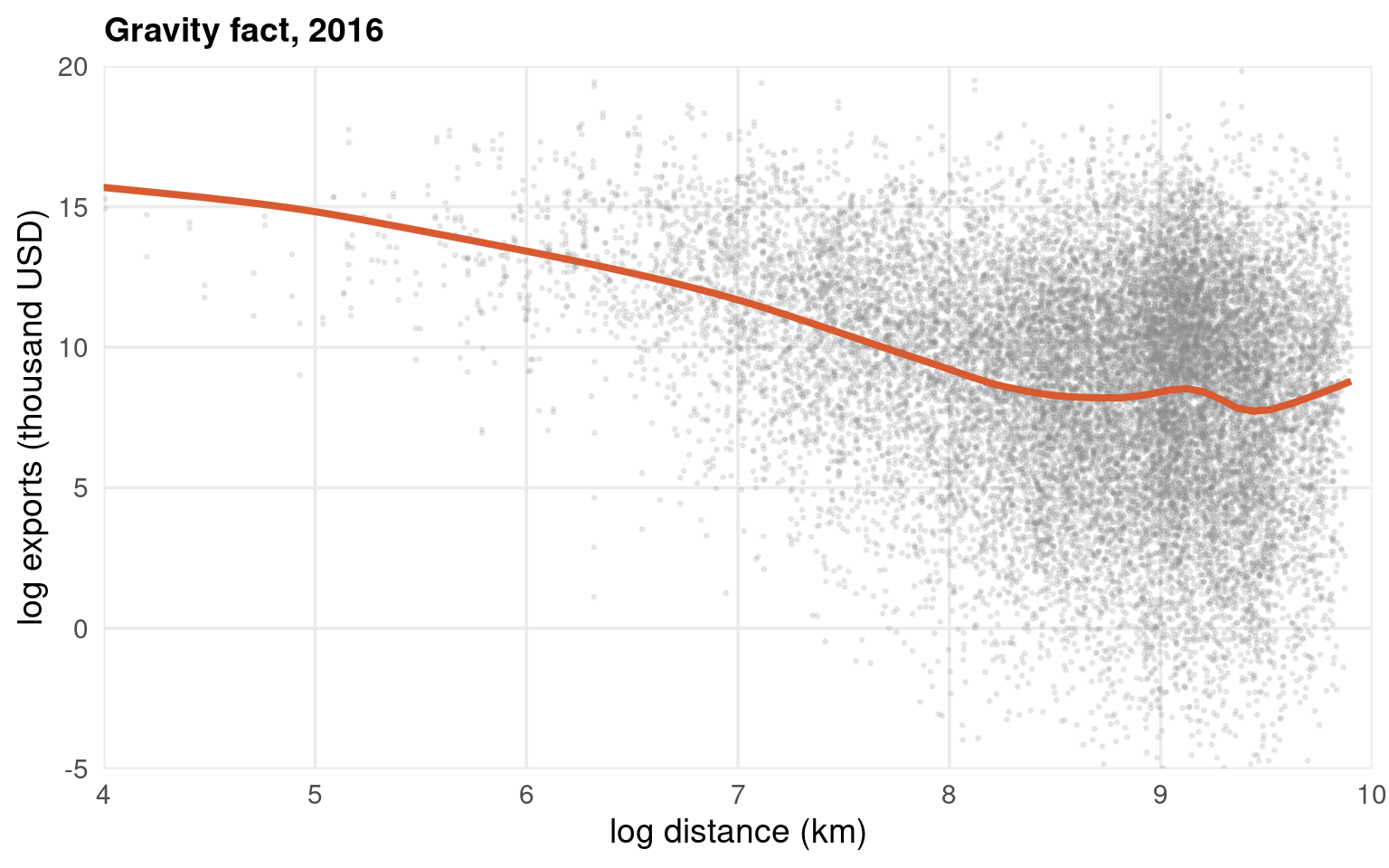
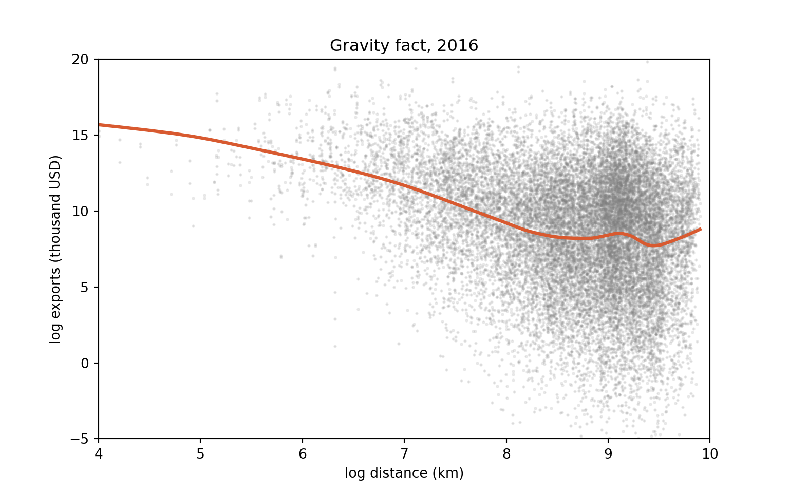
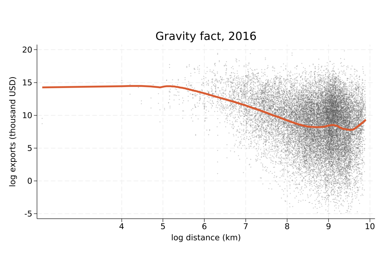
Exports against distance, 2016, all pairs with a positive flow. The line is a Cleveland lowess smoother with span 0.3 — identical in all three tabs, as are the axis limits and the ticks.
The scatter clips at \(\log X = -5\) and \(\log X = 20\) in every tab. Stata’s yscale(range()) only extends an axis, so its scatter is restricted with an if condition instead — the smoother still runs on the full sample.
The Structural Form
Gravity is not an analogy. It falls out of CES demand with iceberg trade costs, and the shape of what it delivers is what the rest of the deck exploits:
1. Preferences. Each country produces one differentiated good (the Armington assumption). Consumers everywhere have CES preferences over the national varieties, with elasticity of substitution \(\sigma > 1\):
2. Trade costs. Shipping from \(i\) to \(j\) melts a fraction of the cargo — the iceberg cost \(\tau_{ij} \ge 1\). Delivering one unit requires shipping \(\tau_{ij}\) of them, so the delivered price is \(p_{ij} = p_i \tau_{ij}\). Nothing else about geography enters the model.
3. Demand. Maximising \(U_j\) subject to spending \(E_j\) gives the CES expenditure share; multiplying by \(E_j\) gives the value of the flow:
4. Separation. Collect terms. Everything about the exporter goes into one factor, everything about the importer into another, and only \(\tau_{ij}\) is genuinely bilateral — which is the boxed equation on the slide.
5. Market clearing. Anderson and van Wincoop close the model by requiring that each country’s output be bought by somebody, \(Y_i = \sum_j X_{ij}\). Substituting the demand equation and solving gives the two resistance terms of the second tab. Their contribution was not the demand system — that is Anderson (1979) — but the observation that the general-equilibrium price terms cannot be dropped from an estimating equation.
Eaton and Kortum (2002) reach an identical trade-share equation from Ricardian technology draws rather than differentiated varieties, with \(\theta\) a Fréchet dispersion parameter instead of \(\sigma - 1\). The gravity structure this deck estimates is common to both, which is why Part V can measure \(\theta\) without committing to either story.
The structural form is multiplicative and separable. Three consequences run through the whole deck:
The exporter and importer terms are fixed effects. Part III never estimates them; it absorbs them.
The elasticity \(\sigma - 1\) is the trade elasticity\(\theta\). One number converts an observed trade cost into a trade flow, and Part V is entirely about measuring it.
Trade costs enter only through \(\tau_{ij}^{-\theta}\). If we can write \(\log \tau_{ij}\) as a function of distance, borders and language, the coefficients we estimate are \(-\theta\) times those elasticities — never the elasticities themselves.
\(\Pi_i\) is outward multilateral resistance and \(P_j\)inward. Neither is observed. Both are defined by a system that references the other, so they must be solved for — which is exactly the fixed point Part VI computes.
Part III takes the cheaper route and absorbs them as fixed effects; that is the whole reason its specification looks the way it does.
Why the border puzzle needed this
McCallum (1995) regressed Canadian province–US state trade on size, distance and a border dummy and found that provinces traded 22 times more with each other than with comparable states. The number was absurd, and it was the estimate a naive gravity regression gives.
Anderson and van Wincoop showed the specification was misspecified, not the world. Omitting \(\Pi_i\) and \(P_j\) biases the border coefficient, because a border raises the cost of one route and lowers the resistance a country faces on every other route. Canada is small and next to a giant, so its inward resistance moves a great deal; the United States is large, so its own barely moves.
Correcting for that asymmetry cut the estimate to a border effect of roughly 10.7 for Canada and 1.5 for the United States — same data, same border dummy, different treatment of a term nobody can observe.
The lesson is not that borders do not matter. It is that in a general-equilibrium system, a coefficient on a bilateral variable is only interpretable once the multilateral terms are controlled for. Part III does that with fixed effects; Part VI does it by solving the system.
Naive Gravity — Log-Linear OLS
Take logs of the Tinbergen form and run least squares. This is where nearly every empirical trade paper before 2006 began, and it is the estimator Parts II and IV dismantle.
Size elasticities near one, a distance elasticity near \(-1.3\), contiguous neighbours trading \(e^{1.01} \approx 2.7\) times more. The fit looks excellent and the three languages agree to six decimals.
Then the last line of each tab runs the same specification by Poisson PML and gets a distance elasticity roughly half the size, on more data. One of those two numbers is wrong, and the fit statistics cannot tell you which.
Two things are wrong with the log-linear estimate, and they are independent.
The Zeros Problem
log(0) is undefined, so every pair that did not trade was dropped before the regression ran — and they were not dropped at random.
Zero flows by wave


Summary for variables: zero
Group variable: year

    year |         N       Sum      Mean
---------+------------------------------
    2000 | 22052.000  5159.000     0.234
    2004 | 22052.000  3630.000     0.165
    2008 | 22052.000  2960.000     0.134
    2012 | 22052.000  2611.000     0.118
    2016 | 22052.000  2404.000     0.109
    2020 | 22052.000  3234.000     0.147
---------+------------------------------
   Total |  1.32e+05 19998.000     0.151
----------------------------------------


2016, by importer GDP quintile (1 = smallest)


Summary for variables: zero
Group variable: gq (5 quantiles of lgdp_d)

      gq |         N      Mean
---------+--------------------
       1 |  4144.000     0.177
       2 |  3996.000     0.147
       3 |  4144.000     0.084
       4 |  3996.000     0.045
       5 |  3996.000     0.011
---------+--------------------
   Total | 20276.000     0.093
------------------------------
The zero share falls from 23.4% in 2000 to 10.9% in 2016, then rises again to 14.7% in 2020. But the decisive cut is the second table: 17.7% of flows into the smallest importers are zero against 1.1% into the largest.
Dropping zeros therefore does not thin the sample evenly — it removes small economies, which is precisely the part of the world a trade-policy question is usually about.
That is only the first defect, and the second has nothing to do with zeros. The model says the level of trade is multiplicative with a mean-one error, and logs do not pass through an expectation:
That second term is harmless only if it is constant. It is not: when the dispersion of \(\eta_{ij}\) varies with the regressors — and trade with small, distant partners is far noisier than trade with large, close ones — it moves with them and lands straight in \(\hat{\boldsymbol\beta}\). It would bias log-OLS even if every pair traded.
Jensen’s inequality, in full
The structural model of the previous slide is a statement about the level of trade, with a multiplicative error that is mean one conditional on the regressors:
By Jensen’s inequality \(\mathbb{E}[\log \eta] \le \log \mathbb{E}[\eta] = 0\), with equality only if \(\eta\) is degenerate. So log-OLS estimates \(\boldsymbol\beta\)plus a term nobody wrote down.
The term is a nuisance only if it is constant. If \(\eta_{ij}\) were homoskedastic, \(\mathbb{E}[\log\eta]\) would be the same number for every pair and would vanish into the intercept. It is not. For a log-normal error with variance \(\sigma^2_{ij}\) the term is exactly \(-\sigma^2_{ij}/2\) — so any pattern in the variance becomes a pattern in the mean of the log, and therefore a bias in every coefficient correlated with it.
That is Santos Silva and Tenreyro’s (2006) argument, and it is a statement about heteroskedasticity, not about zeros. The two defects are independent: dropping zeros is a selection problem, Jensen is a functional-form problem, and log-OLS has both.
It is visible in the residuals of the fit on the previous slide. Group them by distance band and the mean log residual is not constant — it is strongly positive for neighbours and negative in the middle bands — while the residual spread widens with distance. That combination is the bias term in the flesh, which is why the Poisson estimate on the same data is roughly half the log-OLS one.
Part II stops arguing and measures it: a simulated world with a known \(\theta\), drawn with exactly this kind of heteroskedastic noise, where log-OLS and PPML can be scored against the right answer.
Part II settles which of the two distance elasticities to believe by building a world where the answer is known in advance.
Gravity is not an analogy. It falls out of CES demand with iceberg trade costs, and the structural form is multiplicative and separable.
Separability means the exporter and importer terms are fixed effects, and the only genuinely bilateral object is \(\tau_{ij}^{-\theta}\).
Estimated trade-cost coefficients are always \(-\theta\) times an elasticity, never the elasticity itself.
Multilateral resistance is real, unobserved, and defined by a fixed point. Ignoring it produced a 22-fold Canadian border effect.
Log-linear OLS has two independent defects: it discards zeros non-randomly, and Jensen’s inequality biases what remains.
Task
R
Python
Stata
Read the panel
data.table::fread
pandas.read_csv
import delimited
Log-linear OLS
fixest::feols
statsmodels.OLS
regress
Robust (HC1) SEs
vcov = "hetero"
cov_type="HC1"
, robust
Poisson PML
fixest::fepois
pyfixest.fepois
ppmlhdfe
Lowess smoother
stats::lowess
statsmodels … lowess
lowess
Quintiles
cut(quantile(...))
pandas.qcut
xtile
Match iter = 0 in R and it = 0 in Python to Stata’s single-pass lowess, or the three curves will not coincide.
Never let log() do your sample selection silently. Count the zeros first, and report how many observations the log specification dropped.
HC1 is the common denominator across all three languages. Two-way clustering by exporter and importer is the right answer for a gravity panel, and Part III does it — but regress cannot, so it needs reghdfe or ppmlhdfe.
CEPII lists countries that did not exist in a given year. Filter on country_exists_o and country_exists_d or a tenth of the panel arrives with missing distance and GDP for countries that plainly have both.
Real data cannot tell us which is right, because the true distance elasticity of world trade is not written down anywhere. Every argument from real data is an argument about plausibility.
So we build a world where the answer is known by construction, run both estimators on it, and see which one finds it again.
Not a toy. The simulated world uses:
60 real countries — the largest traders with complete CEPII coverage
their real bilateral distances, contiguity and common language
their real 2016 population and GDP per capita as labour and productivity
an equilibrium solved until every market clears to within \(2\times10^{-13}\)
What is invented is only what has to be: the trade elasticity\(\theta = 4\), the trade-cost elasticities, and the noise. Everything the estimator sees looks like the data from Part I. Everything it is trying to recover, we chose.
That the DGP reproduces the awkward features of real trade data — zeros, extreme skew, and variance that grows faster than the mean
That log-OLS misses the truth, in a direction and by an amount we can measure
That PPML does not
That this is a statement about the estimator, not about one lucky draw — which needs a Monte Carlo, not a single regression
Armington: each of \(N = 60\) countries produces one variety, labour is the only factor, and the unit cost is \(c_i = w_i / A_i\). Expenditure shares are CES:
with \(\tau_0 = 1.55\), \(\delta_d = 0.25\), \(\delta_c = -0.12\), \(\delta_l = -0.09\), \(\tau_{ii} = 1\), and \(\varepsilon_{ij} = \varepsilon_{ji} \sim N(0, 0.15^2)\) — the unobserved part of trade costs, which is the gravity error term.
Because the model is separable, the coefficients a regression can recover are \(-\theta\) times these elasticities:
Two things are deliberate. The mean is correct — \(\mathbb{E}[X_{ij}] =
\lambda_{ij}\) — so any estimator that models the mean is consistent. And the variance grows with distance, so \(\mathbb{E}[\log \nu_{ij}]\) moves with a regressor. That is the Jensen mechanism of Part I, now switched on deliberately.
Poisson sampling also produces the zeros, without any separate selection rule.
DGP — Code Implementation
The world was drawn once, from seed 14159. Every tab reads the same two files and checks that they are internally consistent.
Code
s <-fread("../data/ctm-sim.csv") # 60 x 60 flows and the truth behind themtr <-fread("../data/ctm-sim-truth.csv") # per-country truth + the DGP parameterso <- s[domestic ==0][, ldist :=log(dist)]# the equilibrium condition, checked rather than assumed:# w_i L_i == sum_j pi_ij w_j L_jw <-setNames(tr$w, tr$iso3); L <-setNames(tr$L, tr$iso3); E <-setNames(tr$E, tr$iso3)sales <- s[, .(sales =sum(pi_true * E[importer])), by = exporter]gap <-max(abs(sales$sales - (w * L)[sales$exporter]))cat(sprintf("market-clearing gap %.2e\n", gap))cat(sprintf("theta %.0f beta_dist %.2f beta_contig %.2f beta_lang %.2f\n", tr$theta[1], -tr$theta[1] * tr$delta_dist[1],-tr$theta[1] * tr$delta_contig[1], -tr$theta[1] * tr$delta_lang[1]))
countries 60 international pairs 3540 zeros 159 (4.5%)
market-clearing gap 1.75e-13 median domestic share 0.811
countries 60   international pairs 3540   zeros 159 ( 4.5%)

market-clearing gap   1.8e-13   median domestic share  0.811

theta  4   beta_dist -1.00   beta_contig  0.48   beta_lang  0.36
DGP Diagnostics — Does It Look Like Trade Data?
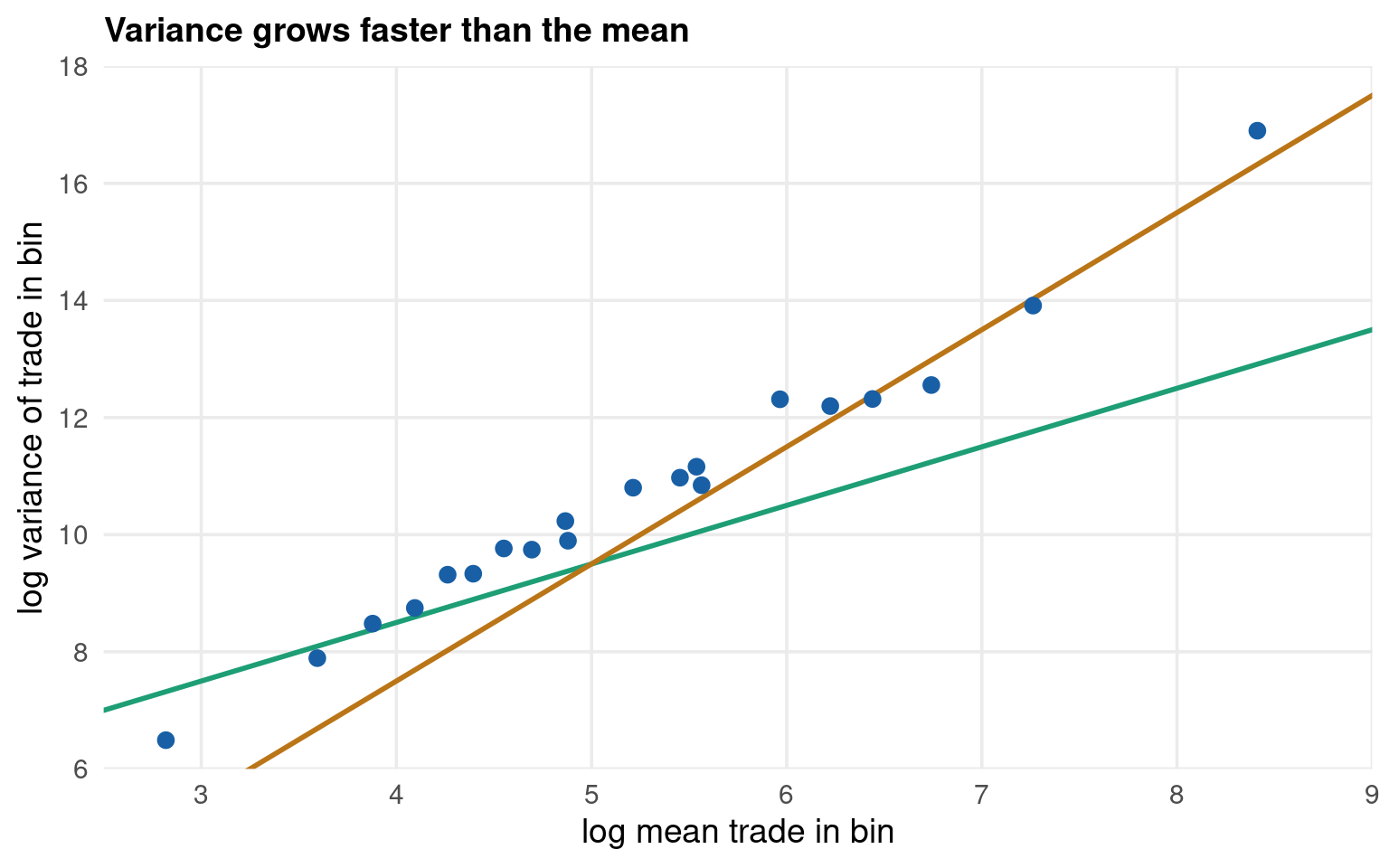
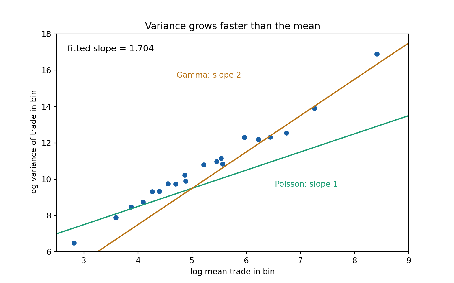
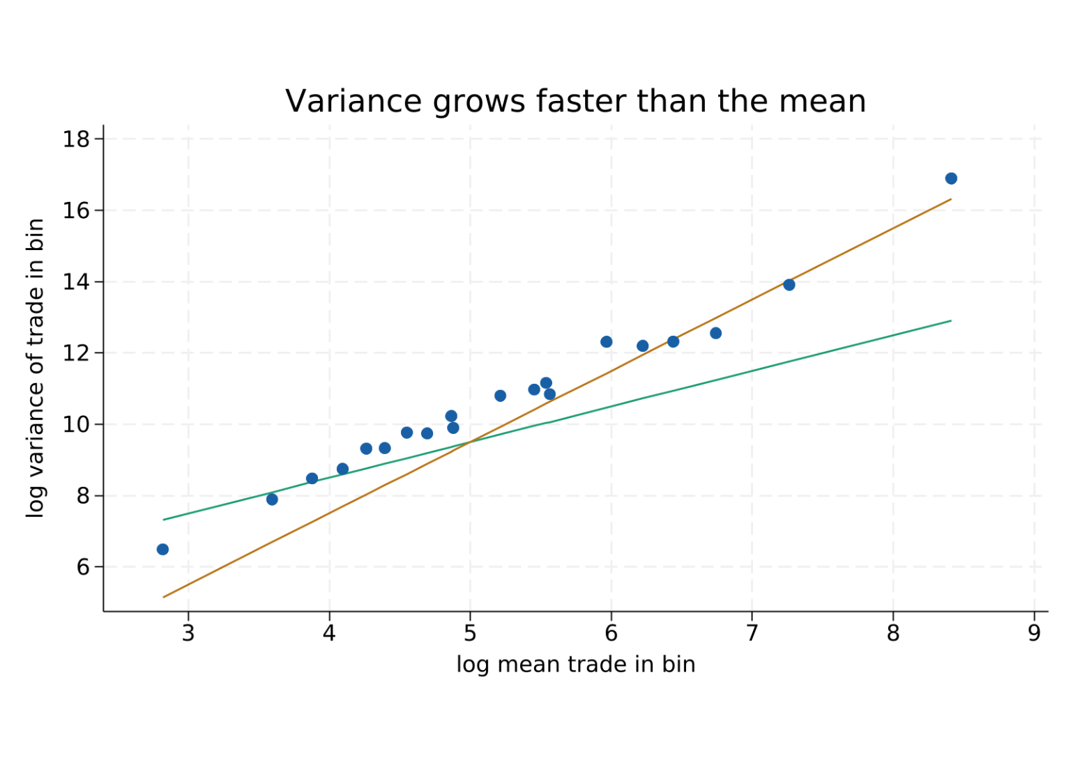
Twenty bins of pairs ordered by their model mean \(\lambda_{ij}\). If the data were Poisson the cloud would lie on the slope-1 line; if Gamma, on slope 2.
Code
o[, bin :=cut(lambda_true, quantile(lambda_true, seq(0, 1, length.out =21)),include.lowest =TRUE, labels =FALSE)]b <- o[, .(m =mean(trade), v =var(trade)), by = bin]b[, `:=`(lm =log(m), lv =log(v))]ref <-data.frame(lm =c(2.5, 9), lv1 =c(2.5, 9) +4.5, lv2 =2*c(2.5, 9) -0.5)ggplot(b) +aes(x = lm, y = lv) +geom_abline(intercept =4.5, slope =1, colour ="#1D9E75", linewidth =1) +geom_abline(intercept =-0.5, slope =2, colour ="#BA7517", linewidth =1) +geom_point(colour ="#185FA5", size =2.6) +coord_cartesian(xlim =c(2.5, 9), ylim =c(6, 18), expand =FALSE) +scale_x_continuous(breaks =3:9) +scale_y_continuous(breaks =seq(6, 18, 2)) +labs(x ="log mean trade in bin", y ="log variance of trade in bin",title ="Variance grows faster than the mean") + theme_lecture
Code
import matplotlib.pyplot as plto["bin"] = pd.qcut(o.lambda_true, 20, labels=False)b = o.groupby("bin").agg(m=("trade", "mean"), v=("trade", "var"))lm, lv = np.log(b.m.values), np.log(b.v.values)slope = np.polyfit(lm, lv, 1)[0]x = np.array([2.5, 9.0])fig, ax = plt.subplots(figsize=(8, 5))ax.plot(x, x +4.5, color="#1D9E75", linewidth=1.6)ax.plot(x, 2* x -0.5, color="#BA7517", linewidth=1.6)ax.scatter(lm, lv, color="#185FA5", s=28)ax.text(0.03, 0.92, "fitted slope = %.3f"% slope, transform=ax.transAxes, fontsize=11)ax.text(0.62, 0.30, "Poisson: slope 1", color="#1D9E75", transform=ax.transAxes, fontsize=10)ax.text(0.34, 0.80, "Gamma: slope 2", color="#BA7517", transform=ax.transAxes, fontsize=10)axopts = ax.set(xlim=(2.5, 9), ylim=(6, 18), xticks=range(3, 10), yticks=range(6, 19, 2), xlabel="log mean trade in bin", ylabel="log variance of trade in bin", title="Variance grows faster than the mean")plt.show()
Regressing log variance on log mean across the bins gives a slope of 1.704 — between Poisson and Gamma, and comfortably above 1. The simulated world has the same awkward shape as the real one: 10.29 skewness in levels, 4.5% exact zeros, and a variance-to-mean ratio that climbs from 95 in the smallest bin to 4 466 in the largest.
Estimation — Poisson Pseudo-Maximum Likelihood
PPML on all 3 540 international pairs, exporter and importer fixed effects, standard errors clustered on the exporter.
Note what PPML is not doing here. Trade flows are continuous, not counts — Poisson is used for its multiplicative mean, and the likelihood is a pseudo-likelihood. The companion deck Duration, Survival and Count Models treats Poisson as a genuine count model, where the variance assumption is a claim about the data and overdispersion has to be tested rather than assumed away.
Log-OLS misses the distance elasticity by \(-0.297\) — it says trade falls with distance a third faster than it truly does. Gamma PML, which fixes Jensen but still cannot take the log of zero, lands within 0.010.
Note what this single draw does not show. Gamma PML is closer than PPML on distance here (\(-0.009\) against \(+0.026\)), and PPML is closer on contiguity and language. One cross-section cannot rank two consistent estimators — the differences between them are sampling noise, while the gap to log-OLS is not. Separating those two things is what the next slide is for.
\begin{tabular}{lrrrr}\hline\hline& Truth & PPML & log-OLS & Gamma PML \\\hline$\log$ distance &$-1.00$&$-0.9740$&$-1.2968$&$-1.0093$\\&&$(0.0235)$&$(0.0347)$&$(0.0328)$\\Contiguity &$0.48$&$0.4972$&$0.2748$&$0.4113$\\&&$(0.0882)$&$(0.0890)$&$(0.0789)$\\Common language &$0.36$&$0.3289$&$0.3430$&$0.3120$\\&&$(0.1145)$&$(0.0914)$&$(0.1071)$\\\hlineObservations && 3540 & 3381 & 3381 \\Exporter FE && Yes & Yes & Yes \\Importer FE && Yes & Yes & Yes \\\hline\hline\end{tabular}
One regression cannot separate bias from luck. So hold the design fixed — the same 60 countries, the same distances — and redraw both the unobserved trade-cost shock \(\varepsilon_{ij}\) and the observation noise, 200 times.
Code
th <- tr$theta[1]; st <- tr$sigma_tau[1]# recover the realised cost shock so it can be replaced by a fresh oneo[, eps0 :=log(tau_true) -log(tr$tau0[1]) - tr$delta_dist[1] *log(dist /min(dist)) - tr$delta_contig[1] * contig - tr$delta_lang[1] * comlang]set.seed(14159)B <-200res <-matrix(NA_real_, B, 6)for (b in1:B) { lam <- o$lambda_true *exp(-th * (rnorm(nrow(o), 0, st) - o$eps0)) nu <-rgamma(nrow(o), shape =1/ o$sigma2_true, rate =1/ o$sigma2_true) d <-copy(o)[, yb :=as.numeric(rpois(nrow(o), lam * nu))] mp <-fepois(yb ~ ldist + contig + comlang | exporter + importer, data = d) mo <-feols(log(yb) ~ ldist + contig + comlang | exporter + importer, data = d[yb >0]) res[b, ] <-c(coef(mp)[c("ldist", "contig", "comlang")],coef(mo)[c("ldist", "contig", "comlang")])}
B = 200 replications

   term      truth  PPML_bias  PPML_rmse   OLS_bias   OLS_rmse


   ldist      -1.00    -0.0081     0.0447    -0.3178     0.3194
  contig       0.48    -0.0071     0.1027    -0.1571     0.1782
 comlang       0.36    -0.0126     0.1083    -0.0466     0.1079
Over 200 replications PPML’s distance elasticity is off by \(-0.003\) with a root mean squared error of 0.044. Log-OLS is off by \(-0.316\) with an RMSE of 0.318 — the entire error is bias, and it is a hundred times PPML’s.
Each language draws its own 200 replications from its own generator, so the three tabs agree to Monte Carlo error rather than to the digit. Across R, Python and Stata the PPML bias comes out as \(-0.0032\), \(+0.0045\) and \(-0.0081\) — every one within a hundredth of zero — while log-OLS returns \(-0.316\), \(-0.311\) and \(-0.318\). The conclusion is identical in all three; the fourth decimal is not, and should not be reported as though it were.
The Verification Toolkit
The Monte Carlo just did something the rest of the deck cannot: it knew the answer in advance. Everywhere else the answer is unknown, and that is where the real risk lives.
A clean run is not a correct run. Every wrong number in this deck’s build history arrived with zero errors, zero warnings and a plausible magnitude.
1. Known truth. Simulate a world whose parameters you chose, then estimate it back. Part II does this for \(\theta\); Part VI’s solver is graded against a counterfactual solved in levels, using productivities the solver never sees. Expensive to build once, decisive forever.
2. The null shock. Feed the model a change of nothing — every shock equal to one — and demand that every result come back exactly one. Parts VI and VII both run this before reporting any counterfactual. It catches normalisation errors, indexing errors and stale state in a single line, and it costs one solve.
3. Accounting identities. Every model here has quantities that must hold regardless of the data: value-added shares reproduce gross output (\(\mathbf{v}'\mathbf{L} = \mathbf{1}'\)), expenditure shares sum to one, value-added exports never exceed gross exports, and Fally’s adding-up requires fitted trade to reproduce observed totals country by country. Check them before looking at the result you care about.
4. Independent re-implementation. Three tabs, three ecosystems, no shared code. When R, Python and Stata agree to four decimals, that agreement is the test suite — not decoration. When they disagree, one of them is wrong and the deck says which.
The order matters. Identities are cheap and catch the crudest errors; known-truth validation is expensive and catches everything else.
Defense 4 caught this one. The R and Python tabs of Part I’s residual analysis reported different numbers for the same computation, and only a value-by-value comparison exposed it.
Code
import pandas as pd, numpy as np, statsmodels.api as smrng = np.random.default_rng(14159)d = pd.DataFrame({"x": np.arange(10.0)})d["y"] =2* d.x +1+ rng.normal(size=10)sub = d[d.x >4] # the filter KEEPS the index 5..9X = pd.DataFrame({"x": sub.x.values}) # a fresh frame: index 0..4fit = sm.OLS(sub.y.values, sm.add_constant(X)).fit()bad = sub.assign(r=fit.resid) # aligns on INDEX -> all NaNgood = sub.assign(r=np.asarray(fit.resid)) # aligns on POSITIONout = ("assign(r=fit.resid) "+str(np.round(bad.r.values, 3)) +"\nassign(r=np.asarray(...)) "+str(np.round(good.r.values, 3)) +"\n\nno error and no warning: a groupby on the first one returns\n""a full table of plausible numbers built from nothing.")import sysnbytes = sys.stdout.write(out +"\n")
assign(r=fit.resid)        [nan nan nan nan nan]
assign(r=np.asarray(...))  [-0.714  0.543  0.656 -0.086 -0.399]

no error and no warning: a groupby on the first one returns
a full table of plausible numbers built from nothing.
Code
sys.stdout.flush()
pandas aligns on the index, not on position. The filtered frame kept its original labels while statsmodels returned a fresh RangeIndex, so every value landed in a row that does not exist. Always np.asarray() before assigning a model’s output back to a filtered frame.
Defense 3 caught this one, in all three languages at once: after a Poisson fit, every ecosystem predicts the linear index by default, and the adding-up identity then fails by 100% instead of \(10^{-7}\).
Code
set.seed(14159)n <-200x <-rnorm(n)y <-rpois(n, exp(1+0.5* x))fit <-glm(y ~ x, family = poisson)# Poisson with an intercept: the fitted MEANS must sum to the observed totalcat(sprintf("observed total %10.2f\n", sum(y)))cat(sprintf("sum of predict(fit) %10.2f <- the LINK\n", sum(predict(fit))))cat(sprintf("sum of type = 'response' %10.2f <- the mean\n",sum(predict(fit, type ="response"))))
observed total 616.00
sum of predict(fit) 197.69 <- the LINK
sum of type = 'response' 616.00 <- the mean
The wrong line is not an error — it is a plausible vector of the wrong quantity. Use predict(type = "response") in R, .predict(type="response") in pyfixest, and predict …, mu after ppmlhdfe …, d in Stata. The same trap has three spellings and one symptom.
Three quiet ways a correct algorithm reports a wrong number:
Stata reads CSVs as float. Seven significant digits. Part II’s market-clearing residual reads \(10^{-8}\) instead of \(10^{-13}\), and a machine-precision equilibrium looks sloppy. set type double in every chunk that needs it — the collectcode preamble does not reliably carry it.
rpois returns an integer matrix in R. Head–Ries multiplies two diagonal elements, overflows, and returns NA with only a warning. storage.mode(X) <- "double" immediately after the draw.
A convergence tolerance is a claim about your answer. The GE solvers here run to \(10^{-12}\) because the validation they are graded against holds to \(10^{-11}\). A looser tolerance would still “converge” — to a different number.
None of this is original; it is standard practice, written down.
Yotov, Piermartini, Monteiro & Larch (2016), An Advanced Guide to Trade Policy Analysis, WTO/UNCTAD — the solved applications this deck follows run exactly these consistency checks. wto.org
Fally (2015), Structural gravity and fixed effects, JIE 97(1) — the adding-up property that defense 3 tests. 10.1016/j.jinteco.2015.05.005
Arkolakis, Costinot & Rodríguez-Clare (2012), New Trade Models, Same Old Gains?, AER 102(1) — the sufficient-statistic identity Part VI checks its solver against. 10.1257/aer.102.1.94
Gentzkow & Shapiro (2014), Code and Data for the Social Sciences: A Practitioner’s Guide — testing and replication discipline for empirical work. web.stanford.edu
The distance elasticity that log-OLS reported in Part I, \(-1.319\), is the kind of number a biased estimator produces. In a world where the truth is \(-1.00\), log-OLS returns \(-1.297\).
The bias is not caused by the zeros. Gamma PML drops exactly the same observations as log-OLS and still lands within \(0.010\) of the truth.
The bias is caused by heteroskedasticity plus the log. Fix the log, and the problem goes away.
PPML is consistent for the conditional mean whatever the variance function is, which is why it survives a variance-to-mean ratio running from 95 to 4 466.
One regression cannot show this. A Monte Carlo can, and it needs to redraw the unobserved trade costs as well as the sampling noise — otherwise it measures the luck of a single design draw.
Task
R
Python
Stata
Poisson PML with FE
fixest::fepois
pyfixest.fepois
ppmlhdfe
Gamma PML with FE
fixest::feglm
sm.GLM + dummies
glm, family(gamma)
Linear with FE
fixest::feols
pyfixest.feols
reghdfe
Cluster on exporter
vcov = ~exporter
vcov={"CRV1":"exporter"}
cluster(expid)
Gamma\((1/\sigma^2,\,\cdot)\), mean 1
rgamma(shape=, rate=)
rng.gamma(shape, scale)
rgamma(a, b)
Comparison table
etable
DataFrame.to_string
esttab, keep()
The three Gamma parameterisations are not the same call. R takes shape/rate, NumPy and Stata take shape/scale. Mean one requires rgamma(1/s2, rate = 1/s2) in R and gamma(1/s2, s2) in the other two.
Coefficients agree across the three languages to four decimals; clustered standard errors do not — Stata and fixest use different finite-sample corrections, so expect the third decimal to move.
pyfixest has no Gamma family. Use statsmodels.GLM with explicit dummies, and remember it is then estimating the fixed effects rather than absorbing them.
A Monte Carlo that redraws only the sampling noise measures the wrong thing. On this design it makes PPML look biased on contiguity by \(+0.094\), purely because the single realised draw of \(\varepsilon_{ij}\) happens to correlate with it.
The naive regression put \(\log Y_i\) and \(\log Y_j\) on the right-hand side as proxies for those two terms. They are not proxies. They are the wrong objects: the exporter term contains \(p_i\), the importer term contains the unobservable \(P_j\), and both move whenever any trade cost anywhere changes.
Fally (2015) makes the point exactly: estimate the model with exporter-time and importer-time fixed effects and those fixed effects are the multilateral resistance terms, not an approximation to them.
Part III switches from CEPII to ../data/ctm-itpde.csv — ITPD-E Release 3.
50 countries, five waves 2000–2016, four broad sectors
12 500 manufacturing observations, of which 250 are domestic
only 31 manufacturing zeros: at this level of aggregation, everybody trades
The domestic rows are the reason for the switch. Every classroom gravity dataset drops trade with oneself; without it the border effect is not identified at all, and Part V’s elasticity has to be borrowed from someone else’s paper.
The price: ITPD-E constructs domestic flows only where production statistics allow, so China, Switzerland, Malaysia and Thailand are not in this sample. Say so when you present it.
What three-way fixed effects absorb, and what is left to estimate
The workhorse specification, in all three languages
Why the diagonal matters, and what it buys
The border effect — a number that made trade economists uncomfortable
The distance puzzle: sixteen years of globalisation, measured
Trade agreements: pair fixed effects, phase-in, and a falsification test
Standard errors: the difference between a \(t\) of 33 and a \(t\) of 2
Three-Way Fixed Effects — What They Absorb
Write the estimating equation with the structure taken seriously:
\(E_{jt}P_{jt}^{\theta}\), inward resistance, tariffs applied by \(j\) to everyone
multilateral resistance is controlled, not modelled
\(\lambda_{ij}\) pair
distance, contiguity, language, colonial history, and every unobserved pair trait
only time-varying bilateral policy is identified
The three cannot all be used at once and still leave distance estimable. Distance is time-invariant, so pair fixed effects absorb it. That is a feature: it means the RTA coefficient in slide 7 is identified from switches within a pair, not from comparing pairs that have an agreement with pairs that never will.
Dropping \(\mu_{it}\) and \(\nu_{jt}\) does not just add omitted-variable bias to the constant. Because \(P_{jt}\) depends on all trade costs, it is correlated with \(\tau_{ijt}\) by construction:
A country that is remote from everyone has a high \(P_j\) and therefore trades more with each individual partner than its size predicts. Omit \(P_j\) and that shows up as a smaller apparent distance effect for remote countries — the bias runs through the same regressor you are trying to measure.
Three-way PPML is not free. With \(N\) countries and \(T\) periods the number of fixed effects grows with the sample, and Weidner and Zylkin (2021) show the resulting incidental-parameter bias is \(O(1/N)\) and does not vanish in the usual asymptotics.
For a 50-country panel the correction matters most for coefficients identified off few switches. The RTA estimates in slide 7 are exactly that case, so treat their magnitude as indicative and their sign and significance as the finding.
The distance elasticity is \(-0.673\) — close to the PPML value Part I found on CEPII, and half the log-OLS estimate. Contiguity adds \(e^{0.488} = 1.63\) times more trade; a trade agreement, \(e^{0.490} = 1.63\) times. Common language and shared colonial history are not significant once the resistance terms are absorbed properly.
Dividing a country’s imports from \(i\) by its purchases from itself cancels the inward multilateral resistance term exactly. What is left is a ratio of trade costs and unit costs — no unobservables.
That identity is the engine of Part V, and it needs \(X_{jj}\).
With the diagonal in the sample, a single dummy separates international from internal trade:
\[
\text{brdr}_{ij} = \mathbf{1}\{i \neq j\}
\]
Its coefficient measures everything that makes crossing a border costly and is not distance, contiguity, language or a trade agreement: customs, currencies, regulation, standards, information, trust.
Without the diagonal, \(\text{brdr}_{ij} = 1\) for every observation and the coefficient does not exist. This is not a refinement. It is the difference between the question being answerable and not.
Internal distance is not observed — a country does not have a bilateral distance to itself. CEPII supplies a population-weighted internal distance\(d_{ii}\), computed from the distribution of population across subnational units, and that is what the diagonal rows carry here.
It is a construct, and the border coefficient is sensitive to it: a larger assumed \(d_{ii}\) makes internal trade look less remarkable and shrinks the border effect. Report the measure you used.
Estimation — Structural Gravity with Internal Trade
The border coefficient is \(-2.325\). Crossing a national frontier divides trade by \(e^{2.325} = \mathbf{10.2}\), holding distance, contiguity, language, colonial ties and trade agreements constant.
Compare that with the popup in Part I: Anderson and van Wincoop’s corrected Canadian border effect was 10.7. Twenty-three years later, different data, different countries, a different estimator — and the same order of magnitude.
Note also what happens to distance once the diagonal is in: the elasticity falls from \(-0.673\) to \(-0.428\). Much of what looked like a distance effect was the jump from internal to international trade.
Trade Agreements — Identification from Switches
Distance cannot be estimated alongside pair fixed effects. Trade agreements can, because pairs change status: 476 pair-wave switches in this panel.
The specification below carries two lags and one lead. Neither is decoration.
Why pair fixed effects force you to add lags
1. What pair fixed effects leave you. Adding \(\mu_{ij}\) absorbs every time-invariant feature of a pair — distance, contiguity, language, colonial history, and whatever else about the relationship never changes. That is the point: those are exactly the things correlated with signing an agreement. But it also means \(\hat\beta\) is identified only from pairs whose status switches inside the sample window. Everything else contributes nothing.
2. Why the contemporaneous dummy asks the wrong question. An agreement is a process, not an event. Tariff schedules phase in over five to ten years, rules of origin take time to bed down, and firms re-organise sourcing on an investment horizon rather than a calendar one. A dummy that switches on in the wave the treaty enters force is asking whether trade jumped immediately. Mostly it does not.
3. What that costs you. With pair fixed effects the pair’s average level of trade is already absorbed, so any part of the response that arrives later is not attributed to the agreement — it sits in the residual, and it is in the post-treatment periods. The contemporaneous coefficient is biased toward zero, and the fixed effects that fixed the endogeneity problem are what create this one. Baier and Bergstrand’s answer is to let the effect accumulate:
The object of interest is then the cumulative effect \(\beta_0 + \beta_1 + \beta_2\), not \(\beta_0\) alone. On this deck’s four-year waves those three terms span a decade, which is roughly the horizon over which agreements actually operate. That is also why the panel is built on four-year waves in the first place: annual data would need eight or ten lags to reach the same horizon, each one estimated off the same 476 switches.
4. The lead is a falsification test, not another lag. Add \(\text{RTA}_{ij,t+1}\). A treaty signed at \(t\) cannot cause trade at \(t-4\), so under the causal reading \(\beta_{+1} = 0\). If it is not zero, one of two things is happening: firms are anticipating the agreement and re-sourcing early, or governments are signing with partners whose trade was already growing — the very selection the pair fixed effects were meant to remove. The test cannot tell you which, and it does not clear on this data. Report it anyway.
5. The Stata mechanics. On a wave panel you must declare the spacing before L. and F. mean anything: xtset pair year, delta(4). Without delta(4) Stata reads the four-year gaps as missing observations and every lag comes back empty — silently, with the regression still running on the contemporaneous term alone.
contemporaneous only :  0.0684  (se 0.0304,  t  2.25)


cumulative over 8 yrs:  0.0879  =>   9.2% more trade

(dropped 2 observations that are either singletons or separated by a fixed effect)
warning: dependent variable takes very low values after standardizing (9.2788e-09)
Iteration 1:   deviance = 2.6689e+06  eps = .         iters = 5    tol = 1.0e-04  min(eta) =  -3.17  P
Iteration 2:   deviance = 6.1342e+05  eps = 3.35e+00  iters = 5    tol = 1.0e-04  min(eta) =  -4.36
Iteration 3:   deviance = 2.3226e+05  eps = 1.64e+00  iters = 5    tol = 1.0e-04  min(eta) =  -5.58
Iteration 4:   deviance = 1.4435e+05  eps = 6.09e-01  iters = 4    tol = 1.0e-04  min(eta) =  -6.65
Iteration 5:   deviance = 1.2500e+05  eps = 1.55e-01  iters = 4    tol = 1.0e-04  min(eta) =  -7.64
Iteration 6:   deviance = 1.2093e+05  eps = 3.36e-02  iters = 3    tol = 1.0e-04  min(eta) =  -8.64
Iteration 7:   deviance = 1.2011e+05  eps = 6.85e-03  iters = 2    tol = 1.0e-04  min(eta) =  -9.64
Iteration 8:   deviance = 1.1995e+05  eps = 1.33e-03  iters = 2    tol = 1.0e-04  min(eta) = -10.62
Iteration 9:   deviance = 1.1992e+05  eps = 2.55e-04  iters = 2    tol = 1.0e-04  min(eta) = -11.58
Iteration 10:  deviance = 1.1991e+05  eps = 5.35e-05  iters = 2    tol = 1.0e-04  min(eta) = -12.50
Iteration 11:  deviance = 1.1991e+05  eps = 1.26e-05  iters = 2    tol = 1.0e-05  min(eta) = -13.39
Iteration 12:  deviance = 1.1991e+05  eps = 3.13e-06  iters = 2    tol = 1.0e-05  min(eta) = -14.26   S
Iteration 13:  deviance = 1.1991e+05  eps = 7.75e-07  iters = 2    tol = 1.0e-06  min(eta) = -15.24   S
Iteration 14:  deviance = 1.1991e+05  eps = 1.82e-07  iters = 2    tol = 1.0e-07  min(eta) = -16.18   S
Iteration 15:  deviance = 1.1991e+05  eps = 3.59e-08  iters = 2    tol = 1.0e-07  min(eta) = -17.04   S
Iteration 16:  deviance = 1.1991e+05  eps = 5.95e-09  iters = 2    tol = 1.0e-09  min(eta) = -17.71   S O
------------------------------------------------------------------------------------------------------------
(legend: p: exact partial-out   s: exact solver   h: step-halving   o: epsilon below tolerance)
Converged in 16 iterations and 46 HDFE sub-iterations (tol = 1.0e-08)
Warning: VCV matrix was non-positive semi-definite; adjustment from Cameron, Gelbach & Miller applied.

HDFE PPML regression                              No. of obs      =      4,898
Absorbing 3 HDFE groups                           Residual df     =         49
Statistics robust to heteroskedasticity           Wald chi2(4)    =       6.48
Deviance             =  119910.8253               Prob > chi2     =     0.1659
Log pseudolikelihood = -78520.82796               Pseudo R2       =     0.9970

Number of clusters (expid)  =         50
Number of clusters (impid)  =         50
                           (Std. err. adjusted for 50 clusters in expid impid)
------------------------------------------------------------------------------
             |               Robust
       trade | Coefficient  std. err.      z    P>|z|     [95% conf. interval]
-------------+----------------------------------------------------------------
     fta_wto |
         --. |   .0194578   .0581872     0.33   0.738     -.094587    .1335026
         L1. |   .0513578   .0249407     2.06   0.039     .0024749    .1002408
         L2. |  -.0550597   .0396874    -1.39   0.165    -.1328455    .0227261
         F1. |   .0988066   .0512231     1.93   0.054    -.0015888     .199202
             |
       _cons |   9.679705   .0597763   161.93   0.000     9.562546    9.796864
------------------------------------------------------------------------------

Absorbed degrees of freedom:
-----------------------------------------------------+
 Absorbed FE | Categories  - Redundant  = Num. Coefs |
-------------+---------------------------------------|
        expy |       100         100           0    *|
        impy |       100         100           0    *|
        pair |      2449        2449           0    *|
-----------------------------------------------------+
* = FE nested within cluster; treated as redundant for DoF computation
Three readings of the same variable.
Contemporaneous only:\(0.068\), a \(7.1\%\) trade increase — far below the \(e^{0.490}=1.63\) from the specification without pair fixed effects. That gap is the endogeneity Baier and Bergstrand identified: countries sign agreements with partners they already trade with.
With phase-in: the effect accumulates to \(0.088\) over eight years. Agreements work slowly.
The lead test: trade rises before the agreement takes effect (\(\hat\beta_{F1} = 0.099\), \(p = 0.054\)), and the contemporaneous term collapses to \(0.019\). That is the falsification test failing to clear — evidence of anticipation, or of agreements being signed with partners whose trade was already growing. Report it; do not bury it.
Inference — What the Standard Errors Depend On
Same coefficient, same data, five variance estimators.
Code
specs <-list(iid ="iid", robust ="hetero", `cluster exporter`=~iso3_o,`cluster pair`=~pair, `two-way exp & imp`=~iso3_o + iso3_d)# ssc(adj = FALSE) drops fixest's small-sample k adjustment, which ppmlhdfe# does not apply -- without it the three languages differ by 15%vt <-rbindlist(lapply(names(specs), function(nm) { f <-fepois(trade ~ fta_wto | exp_y + imp_y + pair, data = i,vcov = specs[[nm]], ssc =ssc(adj =FALSE))data.table(vcov = nm, estimate =coef(f)["fta_wto"], se =se(f)["fta_wto"],t =coef(f)["fta_wto"] /se(f)["fta_wto"])}))print(vt, row.names =FALSE)
The point estimate never moves. The \(t\) statistic runs from 37.5 to 2.1.
Assuming independence across 12 250 observations that are 50 countries observed five times is not a small sin — it overstates precision by a factor of 15. Cameron, Gelbach and Miller’s two-way estimator is the default for gravity because a shock to Germany’s exports hits 49 observations at once and a shock to Germany’s imports hits another 49.
Two things about the code are worth more than the table. First, ppmlhdfehas no unadjusted option — it reports robust standard errors and nothing else, so the misleading first row cannot be produced in Stata at all. Second, fixest and pyfixest apply a small-sample \(k\) correction that ppmlhdfe does not; without ssc(adj = FALSE) the same estimator reports \(0.0320\) in R and \(0.0279\) in Stata, a \(15\%\) gap that looks like a bug and is a convention.
Exporter-time and importer-time fixed effects are the multilateral resistance terms. Not proxies for them.
Adding the domestic diagonal changes the distance elasticity from \(-0.673\) to \(-0.428\) and makes the border effect estimable at all: 10.2, against Anderson and van Wincoop’s 10.7.
Estimated wave by wave, the distance elasticity rose between 2000 and 2016 instead of falling — the distance puzzle. Containers and air freight did not make geography less relevant. The estimation exercises in Part IX ask you to reproduce it in a five-line loop.
Pair fixed effects cut the apparent RTA effect from \(63\%\) to \(7\%\). Most of the raw correlation was selection, exactly as Baier and Bergstrand argued.
Always run the lead. Here it is significant at \(10\%\), and honest reporting means saying so.
The choice of variance estimator moves \(t\) from 33 to 2 without touching a single coefficient.
Task
R
Python
Stata
Three-way FE PPML
fepois(... \| a+b+c)
pf.fepois("... \| a+b+c")
ppmlhdfe, absorb(a b c)
Two-way cluster
vcov = ~iso3_o + iso3_d
vcov={"CRV1":"iso3_o + iso3_d"}
cluster(expid impid)
Interacted FE
paste(iso3_o, year) or iso3_o^year
string concat
egen group()
Lags on 4-year waves
shift(x, 1), by = pair
groupby.shift(1)
xtset pair year, delta(4) then L.
Model comparison
etable
DataFrame
esttab
xtset pair year, delta(4) is required before L. and F. on a four-year wave panel. Without delta(4) Stata treats the gaps as missing and every lag is empty.
Two-way clustering needs enough clusters in both dimensions. Fifty exporters and fifty importers is adequate; ten would not be.
Interacting fixed effects by pasting strings is fine in R and Python but Stata needs a numeric group — egen expy = group(iso3_o year).
Internal distance is a construct. The border effect is sensitive to it, so state which measure you used; here it is CEPII’s population-weighted distw_harmonic.
If a coefficient is identified off a handful of switches, quote Weidner and Zylkin and treat the magnitude as indicative.
Part IV — Estimator Choice & Diagnostics
Part IV — Which Pseudo-Likelihood?
Part II settled that log-OLS is biased and PPML is not. It did so in a world built to make Poisson the right answer.
Real data is not built by anyone. Part IV asks the question a referee asks: how do you know Poisson is the right pseudo-likelihood here?
They differ only in the assumed variance function \(V(\mu)\). And Gourieroux, Monfort and Trognon’s result is that any of them is consistent as long as the conditional mean is correctly specified — the variance function affects efficiency, not consistency.
So the diagnostic question splits in two:
Is \(\mu_{ij} = \exp(\mathbf{x}_{ij}'\boldsymbol\beta)\) the right mean? → RESET
If so, which \(V(\mu)\) is closest to the truth? → efficiency
The family, and what each member weights
All four on the same data, and how far apart they land
The RESET test — the only one of these that can reject
Separation: when the estimate does not exist at all
What to report
Back to ../data/ctm-gravity.csv, the 2016 CEPII cross-section: 18 632 international pairs among 150 countries, 1 525 of them zero.
Slide 5 switches to ITPD-E services, which is the only sector in either file where separation occurs naturally.
Reading down the table, the weight on a large flow falls. Gaussian PML is dominated by the United States and China; Gamma PML treats a \(\$10\,000\) flow between two small countries as equally informative as a \(\$400\) billion one.
Poisson sits between them, which is one reason it is the default — but only one reason, and not the important one.
Three properties, none of which is “trade is a count”:
Consistency under a correct mean, whatever the true variance is.
It admits zeros without transformation, so the sample is not selected.
Its first-order condition delivers an exact adding-up property: with exporter and importer fixed effects, predicted total exports equal actual total exports for every country. Fally (2015) showed this is what makes the fitted fixed effects be the multilateral resistance terms.
That third property is why Part VI can take PPML estimates straight into a general-equilibrium counterfactual. No other member of the family has it.
Negative binomial PML is common in applied trade work and is a mistake here.
Its estimates are not invariant to the units of the dependent variable: measure trade in dollars rather than thousands of dollars and the coefficients change. For a genuine count that is harmless, because the units are fixed by nature. For trade values it is not, and Bosquet and Boulhol (2014) show the sensitivity is large in practice.
Gamma PML sits with log-OLS, not with Poisson — because \(V(\mu)=\mu^2\) gives every pair the same weight, and the small, distant, noisy flows that dominate the count then dominate the estimate too. In Part II’s simulated world Gamma was almost exactly right. Here it is not.
Both facts are consistent, and together they make the point: the choice of \(V(\mu)\) is an empirical question, not a convention.
Why Absorbing Beats Dummies
That table has 274 fixed effects in it — one per exporter and importer — and not one of them was printed, because not one of them was wanted. Two ways to get rid of them: estimate them and ignore them, or never form them at all.
The three tabs below time both routes on the same data and print the numbers. Read the timings off your run: they are machine- and load-dependent, and the ratio is not the point. The point is that the coefficient is identical.
Frisch–Waugh–Lovell. For a regression on \(\mathbf{X}\) and a matrix of dummies \(\mathbf{D}\), the coefficient on \(\mathbf{X}\) is unchanged if you instead residualise both sides on \(\mathbf{D}\) first:
This is an identity, not an approximation — which is why the timings below buy speed at no cost in accuracy.
With one fixed effect, \(\mathbf{M}_{\mathbf{D}}\mathbf{X}\) is just “subtract the group mean”: one pass over the data, no matrix anywhere. With two or more the projections do not commute, and there is no one-pass formula. But projecting alternately — demean by exporter, then by importer, then by exporter again — converges to the joint projection:
That is the method of alternating projections. Each sweep costs \(O(n)\), and the dummies are never formed.
For a non-linear model, wrap it inside the IRLS loop: each Poisson iteration is a weighted least-squares problem, so absorb the fixed effects inside every iteration. That is exactly what fepois, pyfixest and ppmlhdfe do.
dummies
absorbing
stored
\(n \times (k + G)\)
\(n \times k\)
per iteration
\(O\!\big(n(k+G)^2\big)\)
\(O(nk^2)\) plus a few \(O(n)\) sweeps
scales with \(G\)
badly
hardly at all
\(G\) is the number of fixed-effect levels. Here \(G\) is 274 and the sample is small; in Part III’s three-way panel \(G\) runs into the thousands, and the dummy route stops being merely slow and starts being impossible.
Code
d16 <- g[domestic ==0& year ==2016&!is.na(dist) &!is.na(gdp_o) &!is.na(gdp_d)]d16[, ldist :=log(dist)]# absorbed: the fixed effects are projected out, never estimatedt_abs <-system.time( fit_abs <-fepois(trade ~ ldist + contig + comlang_off + comcol | iso3_o + iso3_d,data = d16))[["elapsed"]]# dummies: 274 extra columns in the design matrix, all of them estimatedt_dum <-system.time( fit_dum <-glm(trade ~ ldist + contig + comlang_off + comcol +factor(iso3_o) +factor(iso3_d),family = poisson, data = d16))[["elapsed"]]cat(sprintf("absorbed %6.2f s ldist %.6f (%d parameters)\n", t_abs, coef(fit_abs)["ldist"], length(coef(fit_abs))))cat(sprintf("dummies %6.2f s ldist %.6f (%d parameters)\n", t_dum, coef(fit_dum)["ldist"], length(coef(fit_dum))))
absorbed    0.80 s   ldist  -0.692285

dummies     8.16 s   ldist  -0.692285
The algorithm is published; only the timings are local.
Frisch & Waugh (1933), Partial Time Regressions as Compared with Individual Trends, Econometrica 1(4) — the partialling-out theorem. 10.2307/1907330
Lovell (1963), Seasonal Adjustment of Economic Time Series, JASA 58(304) — its general form. 10.1080/01621459.1963.10480682
Guimarães & Portugal (2010), A simple feasible procedure to fit models with high-dimensional fixed effects, Stata Journal 10(4) — iterative demeaning. 10.1177/1536867X1001000406
Gaure (2013), OLS with multiple high dimensional category variables, Computational Statistics & Data Analysis 66 — the method of alternating projections and its convergence. 10.1016/j.csda.2013.03.024
Correia (2017), Linear Models with High-Dimensional Fixed Effects: An Efficient and Feasible Estimator — reghdfe. scorreia.com
Correia, Guimarães & Zylkin (2020), Fast Poisson estimation with high-dimensional fixed effects, Stata Journal 20(1) — absorbing inside IRLS, i.e. ppmlhdfe. 10.1177/1536867X20909691
Same coefficient to six decimals in every tab, by both routes. The fixed effects were never the object of interest, and absorbing them is not a shortcut — it is the same estimator, computed without building something you were going to throw away.
All four estimators above are consistent if the conditional mean is \(\exp(\mathbf{x}'\boldsymbol\beta)\). Santos Silva and Tenreyro’s RESET checks exactly that, and nothing else.
Fit the model, keep the linear predictor \(\hat{y}_{ij} = \mathbf{x}_{ij}'\hat{\boldsymbol\beta}\), then re-estimate with its square added:
Reject when the \(t\) statistic on \(\hat\gamma\) exceeds the usual critical value. Rejection says the exponential mean is misspecified — some non-linearity in \(\mathbf{x}\) has been left out.
RESET test:  H0 = exponential mean correctly specified

estimator    gamma       t             p
  Poisson -0.01471  -2.595  9.451000e-03
  log-OLS -0.03587 -35.739 9.633000e-280

reject H0 at 5% when |t| > 1.96
Code
sys.stdout.flush()
Code
quietly import delimited "../data/ctm-gravity.csv", clear varnames(1)quietlykeepif domestic == 0 & year == 2016 & dist < . & gdp_o < . & gdp_d < .quietlygenerate ldist = ln(dist)quietlygenerate ltrade = ln(trade) if trade > 0quietlyegen expid = group(iso3_o)quietlyegen impid = group(iso3_d)display"RESET test: H0 = exponential mean correctly specified"display" estimator gamma t"* the d option saves the sumof the fixed effects; predict, xbd needs it, and* xbd (notxb) is what makes the linear predictor include themquietly ppmlhdfe trade ldist contig comlang_off comcol, absorb(expid impid) vce(robust) dquietlypredictdoubleyh, xbdquietlygeneratedouble yh2 = yh^2quietly ppmlhdfe trade ldist contig comlang_off comcol yh2, absorb(expid impid) vce(robust)display %13s "Poisson" %11.5f _b[yh2] %11.3f _b[yh2]/_se[yh2]quietlydropyh yh2quietly reghdfe ltrade ldist contig comlang_off comcol, absorb(expid impid) vce(robust) residquietlypredictdoubleyh, xbdquietlygeneratedouble yh2 = yh^2quietly reghdfe ltrade ldist contig comlang_off comcol yh2, absorb(expid impid) vce(robust)display %13s "log-OLS" %11.5f _b[yh2] %11.3f _b[yh2]/_se[yh2]display"reject H0 at 5% when |t| > 1.96"
RESET test:  H0 = exponential mean correctly specified

    estimator      gamma          t

      Poisson   -0.01471     -2.595

      log-OLS   -0.03587    -35.448

reject H0 at 5% when |t| > 1.96
Both specifications are rejected, and the difference in degree is the finding.
PPML gives \(t = -2.60\): a rejection, but a marginal one on 18 632 observations, where any test has enormous power. Log-OLS gives \(t = -35.7\) and a \(p\) value with 280 leading zeros — the log-linear mean is not approximately wrong, it is comprehensively wrong.
RESET is the diagnostic to run before arguing about standard errors. An estimator whose mean function is rejected does not have a standard error worth computing.
Suppose every observation for which some fixed effect is active has \(X_{ij} = 0\). The Poisson likelihood is then maximised by driving that fixed effect to \(-\infty\):
The maximum does not exist in the interior. There is no finite estimate, no standard error, and no amount of iteration will find one.
Correia, Guimarães and Zylkin (2021) show this is not a curiosity: with high-dimensional fixed effects and many zeros it happens routinely, and a solver that merely stops iterating will report whatever it happened to reach.
The affected observations carry no information about \(\boldsymbol\beta\) and must be dropped — which is the correct fix, not a compromise.
Three languages, one problem, three different ways of telling you:
ppmlhdfe says dropped 10 observations that are either singletons or separated by a fixed effect — and it checks for separation before iterating, using the Correia–Guimarães–Zylkin algorithm.
fixest reports fixed-effects removed because of only 0 outcomes.
pyfixest raises a UserWarning.
All three then produce identical coefficients on the remaining 9 149 observations. The distance elasticity for services is \(-0.587\).
The danger is not these three. It is a solver that silently returns a large negative fixed effect and a coefficient computed from observations that contain no information.
Every PML in this family is consistent if the mean is right. They differ in \(V(\mu)\), which determines efficiency and how much weight small flows get.
On the 2016 cross-section, Gamma PML lands with log-OLS at \(-1.30\) while Poisson lands at \(-0.69\). In Part II’s simulated world Gamma was almost exactly right. The correct variance function is an empirical question.
Poisson’s unique advantage is not that trade is a count. It is the adding-up property: fitted exports equal actual exports country by country, which is what makes the fixed effects usable as multilateral resistance in Part VI.
Run RESET. Here it rejects log-OLS at \(t = -35.7\) and PPML at \(t = -2.60\) — the same verdict, three orders of magnitude apart in severity.
Check separation. With many zeros and high-dimensional fixed effects there may be no finite maximum, and the affected observations must go.
Do not use negative binomial PML on trade values: it is not scale-invariant.
Task
R
Python
Stata
Poisson PML
fepois
pf.fepois
ppmlhdfe
Gamma / Gaussian PML
feglm(family=)
sm.GLM + dummies
glm, family() link(log)
Linear predictor
predict(type="link")
.predict()
predict, xb / xbd
RESET
refit with yh2
refit with yh2
refit with yh2
Separation check
note in output
UserWarning
reported by ppmlhdfe
Match Stata’s SEs
ssc(adj = FALSE)
pf.ssc(k_adj=False)
default
feglm with a Gamma or log-link Gaussian family needs glm.iter = 200; the default 25 iterations silently stops short and reports a non-converged fit with a warning that is easy to miss.
Both Stata commands need help before predict, xbd will work: ppmlhdfe requires the d option at estimation and reghdfe requires resid``**. Without thempredicterrors; worse, plainxb` succeeds silently and gives a linear predictor with the fixed effects missing**, which turned the Poisson RESET statistic from \(-2.60\) into \(-1.57\).
Compute the RESET regressor from the linear predictor, not from fitted levels — squaring \(\exp(\mathbf{x}'\hat\beta)\) overflows on large flows.
Separation is a property of the data and the fixed effects together. Adding a fixed effect can create it; this deck’s manufacturing sample has none and its services sample has three cells.
Report the number of observations each estimator actually used. In the table above it ranges from 17 107 to 18 632 for the same “sample”.
The comparison table shows coefficients only, deliberately. For Gamma and log-link Gaussian, fixest::feglm’s robust standard errors do not match statsmodels or Stata’s glm — they treat the dispersion parameter differently. The point estimates agree to four decimals in all three; the robust standard errors do not, and a slide that showed both without saying so would be quietly misleading.
Parts I to IV estimated coefficients on distance, contiguity and trade agreements. Every one of them is \(-\theta\)times an elasticity of trade costs. Without \(\theta\), none of them can be turned into a policy statement.
And in Part VI, \(\theta\) alone determines the gains from trade:
Halve \(\theta\) and you double the welfare effect of every counterfactual. Arkolakis, Costinot and Rodríguez-Clare showed that across a whole class of models, the domestic share and \(\theta\) are sufficient statistics for welfare. Everything else in the model washes out.
So a factor-of-two disagreement about \(\theta\) is a factor-of-two disagreement about the value of the world trading system.
And it is the same \(\theta\) whatever story you believe about where trade comes from. Armington, Eaton–Kortum and Melitz–Chaney are three different micro-foundations with one common reduced form:
That is the ACR equivalence, and it is why this part can measure \(\theta\) without first committing to a model — and why the Melitz machinery in Part IX does not change any of Part VI’s welfare arithmetic.
Three theories, one number
Three completely different stories about why trade responds to costs, and one common elasticity:
Armington — national product differentiation with CES demand. \(\theta = \sigma - 1\), the substitution elasticity minus one.
Eaton–Kortum — Ricardian comparative advantage with Fréchet productivity draws. \(\theta\) is the dispersion of those draws: low dispersion means countries are similar and reallocation is easy, so trade responds strongly to cost.
Melitz–Chaney — firm heterogeneity with a Pareto productivity distribution. \(\theta\) is the Pareto shape, and the response runs through the extensive margin — which firms export at all — rather than through how much each one ships.
Arkolakis, Costinot and Rodríguez-Clare (2012) showed that across this whole class, welfare depends on the data only through the domestic expenditure share and \(\theta\). Everything that distinguishes the three models washes out of the welfare formula.
What the literature reports
Head and Mayer’s (2014) meta-analysis collects hundreds of estimates, and the distribution is wide: the median sits around 5, most estimates fall between 3 and 8, and published values run from below 2 to above 12.
That dispersion is not sampling noise. It is method, sector and sample — which is precisely why this part re-runs the estimators on a world where the answer is known, so the part of the spread that is bias can be separated from the part that is real.
\(\theta\) multiplies trade costs, and trade costs are unobserved:
A gravity regression identifies the product\(\theta\delta_d\), never \(\theta\) alone. To separate them you need one of:
a trade cost you can observe in levels — a tariff (Caliendo–Parro)
the domestic diagonal, which pins \(\tau_{ii} = 1\) (Head–Ries)
an assumption about \(\delta\) from outside the data
There is no fourth option, and every estimate of \(\theta\) in the literature rests on one of these three.
Three classical estimators, each applied twice — once to the simulated world, where \(\theta = 4\) by construction, and once to real manufacturing data, where nobody knows:
Head–Ries — the ratio identity, which needs the domestic diagonal
Tetrads — differencing away both fixed effects with a reference pair
Caliendo–Parro — triple differences on bilateral tariffs
Then all of them on one table against the known truth. The spread is the lesson.
The simulated data now carries three worlds, all drawn from seed 14159:
The third exists because Caliendo–Parro’s triple difference is built to cancel anything separable into an exporter effect and an importer effect. Symmetric iceberg costs cancel. So does a uniform import surcharge by one country. Only genuinely pair-specific, direction-specific policy survives — which is exactly what a tariff schedule is, and exactly why they used tariffs.
Head–Ries — The Ratio Identity
Take the structural gravity equation and form the ratio of the two directions of trade between \(i\) and \(j\), divided by both countries’ internal trade:
Every exporter and importer term cancels — unit costs, multilateral resistance, expenditure, all of it. With \(\tau_{ii} = \tau_{jj} = 1\) the geometric-mean bilateral trade cost is:
No regression, no fixed effects, no unobservables — but it delivers \(\tau\)given\(\theta\), not \(\theta\) itself. And it is impossible without \(X_{ii}\), which is why Part III switched to ITPD-E.
On the simulated world the estimator is unbiased in shape but not in level: it correlates 0.73 with the true trade costs and its mean is 5.64 against a truth of 4.85. On real manufacturing data with \(\theta = 4\) imposed, the cheapest pairs are Japan–Taiwan (1.03), Singapore–Taiwan (1.03) and Belgium–Netherlands (1.05); the costliest are Costa Rica–Iran (36.3) and Costa Rica–Kazakhstan (20.7).
Those rankings are believable. The levels are not robust: raise \(\theta\) from 4 to 8 and every trade cost falls by roughly half, because \(\theta\) enters as \(1/(2\theta)\). Head–Ries converts an assumption about \(\theta\) into a number about \(\tau\); it does not test it.
Tetrads — Differencing Away Both Fixed Effects
Pick a reference exporter \(k\) and a reference importer \(\ell\), with \(k \neq \ell\). Then form the double ratio:
\(i\) appears once in each of numerator and denominator, so its exporter term cancels; \(j\) likewise. Taking logs gives a regression with no fixed effects at all:
Head, Mayer and Ries introduced this to study colonial trade, where the object of interest was how bilateral costs evolved and the fixed effects were a nuisance. It identifies \(\theta\delta_d\), the same product a gravity regression gives — so it does not solve the identification problem, it sidesteps the fixed effects.
Two practical warnings: the reference pair must have positive trade in all four cells, and the constructed observations reuse the same flows repeatedly, so the errors are mechanically correlated and naive standard errors are too small.
Tetrads — Code
Code
tot <-rowSums(M) +colSums(M)ord <-order(-tot)kref <- ord[1]; lref <- ord[2] # two largest traders, k != ltet <-CJ(i =1:NN, j =1:NN)[i != j & i != kref & j != lref & i != lref & j != kref]tet[, y :=log((M[cbind(i, j)] * M[kref, lref]) / (M[cbind(i, rep(lref, .N))] * M[cbind(rep(kref, .N), j)]))]tet[, x :=log((D[cbind(i, j)] * D[kref, lref]) / (D[cbind(i, rep(lref, .N))] * D[cbind(rep(kref, .N), j)]))]tet <- tet[is.finite(y) &is.finite(x)]summary(lm(y ~ x, data = tet))
SIMULATED WORLD reference CHN / USA n = 3097
slope -1.3419 (se 0.0341) truth -theta*delta_d = -1.00
ITPD-E MANUFACTURING 2016 reference USA / DEU n = 2249
ITPD-E MANUFACTURING 2016   reference USA / DEU

      Source |       SS           df       MS      Number of obs   =     2,249
-------------+----------------------------------   F(1, 2247)      =   2376.10
       Model |  3898.66465         1  3898.66465   Prob > F        =    0.0000
    Residual |  3686.83772     2,247  1.64078225   R-squared       =    0.5140
-------------+----------------------------------   Adj R-squared   =    0.5137
       Total |  7585.50237     2,248   3.3743338   Root MSE        =    1.2809

------------------------------------------------------------------------------
           y | Coefficient  Std. err.      t    P>|t|     [95% conf. interval]
-------------+----------------------------------------------------------------
           x |  -1.150105   .0235942   -48.75   0.000    -1.196373   -1.103836
       _cons |    .202202   .0298456     6.77   0.000     .1436741    .2607299
------------------------------------------------------------------------------

  => theta * delta_d = 1.1501
On the simulated world the tetrad slope is \(-1.342\) where the truth is \(-1.000\). The estimator is not unbiased — and the reason is the whole of Part I: this is ordinary least squares on a log ratio. Jensen’s inequality does not care that four flows were combined first.
On real data the tetrad slope is \(-1.150\), so \(\theta\delta_d \approx 1.15\). With \(\delta_d = 0.25\) that would be \(\theta \approx 4.6\); with \(\delta_d = 0.2\), \(\theta \approx 5.8\). The product is identified; the split is not.
Each country appears once as exporter and once as importer in the numerator, and once in each role in the denominator. Every country-level term cancels — and so does any symmetric part of \(\tau\).
With observed applied tariffs \(t_{ij}\) entering as \(\tau_{ij} = \tilde\tau_{ij}(1 + t_{ij})\):
The slope is\(-\theta\). No \(\delta\), no assumption, no diagonal — this is the one estimator that identifies \(\theta\) on its own.
Its price is data: it needs bilateral applied tariffs that differ by direction. A symmetric trade cost, or a uniform surcharge by one country, cancels along with everything else.
Caliendo-Parro on the tariff world:  triplets 4598
  slope -3.1015 (se 0.3132)   =>  theta = 3.1015      truth = 4

the same moment, estimated by PPML instead of OLS on logs:
  theta = 3.4164 (se 0.7931)   on all 3540 pairs

baseline world, where trade costs are symmetric:
  sd of the right-hand side = 1.12e-16   -- the moment is empty
Code
sys.stdout.flush()
Code
quietly import delimited "../data/ctm-sim.csv", clear varnames(1)quietlykeepif domestic == 0quietlygeneratedouble lt = ln(1 + tariff)quietlyegen expid = group(exporter)quietlyegen impid = group(importer)display"the Caliendo-Parro moment, estimated by PPML rather than OLS on logs:"ppmlhdfe trade_tar lt, absorb(expid impid) vce(robust)display" theta = " %6.4f -_b[lt] " (se " %6.4f _se[lt] ") truth = 4"
Three ways of using the same identifying variation, on data where \(\theta = 4\):
Estimator
\(\hat\theta\)
Standard error
Triple differences, OLS on log ratios
3.27
0.32
PPML with tariffs and both fixed effects
3.42
0.79
(R, Python and Stata each draw their own 6 000 random triplets, so the OLS row moves by about \(\pm 0.2\) between the tabs; the PPML row uses every pair and is identical in all three.)
The triple difference is a log-ratio estimator, so it carries the Part I bias; the PPML version does not, but pays for it in precision because a \(0\)–\(20\%\) tariff is a weak instrument for trade costs that range over a factor of ten.
The last line of each tab is the important one. On the baseline world, where trade costs are symmetric, the right-hand side has a standard deviation of about \(10^{-16}\) — the moment is numerically empty. Caliendo–Parro does not fail gracefully on symmetric data; it produces a slope of \(-8.6 \times 10^{13}\) and a standard error to match.
Sector by Sector — Elasticities and Coverage
Everything so far used manufacturing. ITPD-E has four broad sectors, and they do not behave alike — nor is the data equally good in all of them.
Code
d5 <-fread("../data/ctm-itpde.csv")S5 <-ssc(adj =FALSE)sector_row <-function(sc) { x <- d5[broad_sector == sc] xi <- x[domestic ==0][, `:=`(ldist =log(dist),exp_y =paste(iso3_o, year),imp_y =paste(iso3_d, year))] p <-fepois(trade ~ ldist + contig + comlang_off | exp_y + imp_y,data = xi, vcov =~iso3_o + iso3_d, ssc = S5) m16 <- x[year ==2016] ir <-sort(unique(m16$iso3_o)); n <-length(ir) M <-as.matrix(dcast(m16, iso3_o ~ iso3_d, value.var ="trade")[, -1])rownames(M) <- ir; storage.mode(M) <-"double" D <-as.matrix(dcast(m16, iso3_o ~ iso3_d, value.var ="dist")[, -1]); rownames(D) <- ir hr <-CJ(i =1:n, j =1:n)[i < j] hr[, tau := ((M[cbind(i,i)] * M[cbind(j,j)]) / (M[cbind(i,j)] * M[cbind(j,i)]))^(1/8)] hr <- hr[is.finite(tau) & tau >0]data.table(sector = sc, domestic = x[domestic ==1& trade >0, .N],hr_pairs =nrow(hr), ppml =coef(p)["ldist"], se =se(p)["ldist"],hr_med_tau =median(hr$tau))}rbindlist(lapply(c("Agriculture", "Mining and Energy", "Manufacturing", "Services"), sector_row))
domestic = country-sector-wave cells with a domestic flow, out of 250
hr_pairs = pairs usable for Head-Ries in 2016, out of 1225
import pyfixest as pfd5 = pd.read_csv("../data/ctm-itpde.csv")S5 = pf.ssc(k_adj=False)def sector_row(sc): x = d5[d5.broad_sector == sc].copy() xi = x[x.domestic ==0].copy() xi["ldist"] = np.log(xi.dist) xi["exp_y"] = xi.iso3_o + xi.year.astype(str) xi["imp_y"] = xi.iso3_d + xi.year.astype(str) p = pf.fepois("trade ~ ldist + contig + comlang_off | exp_y + imp_y", data=xi, vcov={"CRV1": "iso3_o + iso3_d"}, ssc=S5) m16 = x[x.year ==2016] ir =sorted(m16.iso3_o.unique()); n =len(ir) M = m16.pivot(index="iso3_o", columns="iso3_d", values="trade").values.astype(float) D = m16.pivot(index="iso3_o", columns="iso3_d", values="dist").values tot = np.nansum(M, 1) + np.nansum(M, 0) o = np.argsort(-tot); k, l = o[0], o[1] i, j = np.meshgrid(np.arange(n), np.arange(n), indexing="ij") i, j = i.ravel(), j.ravel() keep = (i != j) & (i != k) & (j != l) & (i != l) & (j != k) i, j = i[keep], j[keep]with np.errstate(divide="ignore", invalid="ignore"): y = np.log((M[i, j] * M[k, l]) / (M[i, l] * M[k, j])) xx = np.log((D[i, j] * D[k, l]) / (D[i, l] * D[k, j])) ok = np.isfinite(y) & np.isfinite(xx) b = np.polyfit(xx[ok], y[ok], 1)[0] iu = np.triu_indices(n, k=1)with np.errstate(divide="ignore", invalid="ignore"): tau = ((M[iu[0], iu[0]] * M[iu[1], iu[1]]) / (M[iu] * M[iu[1], iu[0]])) ** (1/8) tau = tau[np.isfinite(tau) & (tau >0)]return [sc, int(((x.iso3_o == x.iso3_d) & (x.trade >0)).sum()), len(tau),round(p.coef()["ldist"], 4), round(p.se()["ldist"], 4),round(b, 4), round(float(np.median(tau)), 2)]st = pd.DataFrame([sector_row(s) for s in ["Agriculture", "Mining and Energy", "Manufacturing", "Services"]], columns=["sector", "domestic", "hr_pairs", "ppml_ldist", "se","tetrad", "hr_med_tau"])out = ("domestic = country-sector-wave cells with a domestic flow, out of 250\n""hr_pairs = pairs usable for Head-Ries in 2016, out of 1225\n""ppml, tetrad both estimate theta * delta_dist; hr_med_tau assumes theta = 4\n\n"+ st.to_string(index=False) +"\n\ntotal domestic coverage: %d of 1000 cells"% st.domestic.sum())import sysnbytes = sys.stdout.write(out +"\n")
domestic  = country-sector-wave cells with a domestic flow, out of 250
hr_pairs  = pairs usable for Head-Ries in 2016, out of 1225
ppml, tetrad both estimate theta * delta_dist; hr_med_tau assumes theta = 4

           sector  domestic  hr_pairs  ppml_ldist     se  tetrad  hr_med_tau
      Agriculture       236       980     -0.9105 0.0933 -2.0720        4.31
Mining and Energy       198       695     -1.2103 0.1776 -2.7963        8.69
    Manufacturing       250      1221     -0.7895 0.0514 -1.1501        3.23
         Services       179       574     -0.6318 0.0670 -1.2903        6.09

total domestic coverage: 863 of 1000 cells
Code
sys.stdout.flush()
Code
settypedouble* the tetrad column is produced in the R and Python tabs; here it would need the* four-way mergeof Part V's tetrad chunk repeated inside a sector loopdisplay"domestic = cells with a domestic flow out of 250; hr_pairs out of 1225"display" sector domestic hr_pairs ppml_ldist se"foreachscin"Agriculture""Mining and Energy""Manufacturing""Services" {quietly import delimited "../data/ctm-itpde.csv", clear varnames(1)quietlykeepif broad_sector == "`sc'"quietlycountif iso3_o == iso3_d & trade > 0scalar ndom = r(N)quietlygenerate ldist = ln(dist)quietlyegen expy = group(iso3_o year)quietlyegen impy = group(iso3_d year)quietlyegen expid = group(iso3_o)quietlyegen impid = group(iso3_d)quietly ppmlhdfe trade ldist contig comlang_off if iso3_o != iso3_d, /// absorb(expy impy) cluster(expid impid)scalar b = _b[ldist]scalarsd = _se[ldist]quietlykeepifyear == 2016quietlykeep iso3_o iso3_d tradepreservequietlykeepif iso3_o == iso3_dquietlyrename trade x_ooquietlykeep iso3_o x_ootempfile domquietlysave`dom'restorequietlymergem:1 iso3_o using`dom', keep(match) nogeneratequietlyrename iso3_d tmpquietlyrename iso3_o iso3_dquietlyrename tmp iso3_oquietlyrename x_oo x_ddquietlymergem:1 iso3_o using`dom', keep(match) nogeneratepreservequietlykeep iso3_o iso3_d tradequietlyrename trade x_jiquietlyrename iso3_o t2quietlyrename iso3_d iso3_oquietlyrename t2 iso3_dtempfile revquietlysave`rev'restorequietlymerge 1:1 iso3_o iso3_d using`rev', keep(match) nogeneratequietlycountif iso3_o < iso3_d & trade > 0 & x_ji > 0 & x_oo > 0 & x_dd > 0display %16s "`sc'" %10.0f ndom %10.0f r(N) %12.4f b %10.4f sd}
domestic = cells with a domestic flow out of 250; hr_pairs out of 1225

          sector  domestic  hr_pairs  ppml_ldist        se

 12.   scalar b = _b[ldist]
 13.   scalar sd = _se[ldist]
 14.
 40.
     Agriculture       236       980     -0.9105    0.0934
Mining and Energy       198       695     -1.2103    0.1777
   Manufacturing       250      1221     -0.7895    0.0514
        Services       179       574     -0.6318    0.0671
Three things, and only the first was expected.
Trade costs differ enormously by sector. The PPML distance elasticity runs from \(-1.21\) in mining and energy — bulk commodities, where freight is most of the cost — to \(-0.63\) in services, much of which travels down a wire. Applying manufacturing’s \(-0.79\) to all four would misprice both ends.
The tetrad estimate is 1.5 to 2.5 times the PPML one in every single sector. Agriculture \(-2.07\) against \(-0.91\); mining \(-2.80\) against \(-1.21\). This is Part V’s central point reproduced four times independently: tetrads are OLS on log ratios, and the bias does not average away.
The data is not equally good. Manufacturing has all 250 domestic cells and 1 221 of 1 225 usable Head–Ries pairs. Services has 179 cells and only 574 pairs — under half. Across all four sectors, 863 of 1 000 domestic cells exist.
That last line is why the services elasticity deserves less confidence than its standard error suggests. The standard error describes sampling variation in the observations you have; it says nothing about the 29% of the diagonal that is missing.
Five Estimators, One Known Truth
The simulated world has theta = 4, exactly.
                         estimator      identifies estimate  error
        Head-Ries (mean tau ratio) tau given theta    4.657  0.657
        Tetrads, OLS on log ratios theta * delta_d    5.368  1.368
 Caliendo-Parro, OLS on log ratios           theta    3.267 -0.733
            Caliendo-Parro by PPML           theta    3.416 -0.584
    PPML on log distance / delta_d           theta    4.549  0.549
Head-Ries and the distance route both need delta_d, which is known here
and unknown in any real dataset.
Five defensible estimators, one world, and answers spanning 3.3 to 5.4 — a factor of \(1.6\), against a truth we chose ourselves.
That range is not a failure of the simulation. It is Head and Mayer’s meta-analysis, reproduced under laboratory conditions: the published spread of \(\theta\) from 2 to 12 is mostly method, not sampling error.
Part VI is where this stops being an academic point. Welfare goes as \(\hat\lambda_{ii}^{-1/\theta}\), so an estimate of 3.3 rather than 5.6 inflates every gain-from-trade calculation by 70%.
Gravity identifies \(\theta\delta\), never \(\theta\). Separating them needs an observed cost in levels, the domestic diagonal, or an outside assumption.
Head–Ries cancels every unobservable exactly and gives \(\tau\)given\(\theta\). Its rankings are credible (Japan–Taiwan 1.03, Costa Rica–Iran 36.3); its levels move by a factor of two when \(\theta\) moves from 4 to 8.
Tetrads remove both fixed effects without estimating them, but identify the same product a gravity regression does.
Caliendo–Parro is the only one that identifies \(\theta\) alone — and it needs bilateral, direction-specific tariffs. On symmetric costs the moment is numerically empty and the estimator returns nonsense rather than a warning.
All three classical estimators are OLS on log ratios, and all three inherit the bias of Part I. On the known-truth world the tetrad slope is \(-1.34\) where the truth is \(-1.00\).
Five estimators, one world, \(\hat\theta\) from 3.3 to 5.6. Report which one you used and what it assumed.
Task
R
Python
Stata
Flows to a matrix
dcast + as.matrix
DataFrame.pivot
reshape wide or merges
Upper triangle
CJ(i,j)[i < j]
np.triu_indices
keep if iso_o < iso_d
Attach \(X_{ii}\) to each row
matrix index M[cbind(i,i)]
M[i, i] fancy index
merge m:1 on a domestic tempfile
Random triplets
replicate(sample(n,3))
rng.choice(n,3)
runiform + sort
The moment by PPML
fepois
pf.fepois
ppmlhdfe
rpois returns integers. Head–Ries multiplies two diagonal flows, which overflows .Machine$integer.max and returns NA with only a warning. Set storage.mode(M) <- "double" immediately after building the matrix.
The tetrad reference exporter and importer must be different countries. Using the same one puts \(X_{kk}\) and \(D_{kk}\) in the formula, and the internal distance is missing — every observation becomes NA and the regression reports 0 non-NA cases rather than anything useful.
Tetrad and triple-difference observations reuse the same flows, so their errors are correlated by construction. Cluster on the reference pair, or bootstrap; do not quote the naive standard error.
Before running Caliendo–Parro, check that the right-hand side varies. If trade costs are symmetric the moment is identically zero and the regression will still return a number.
Head–Ries needs \(X_{ij}\), \(X_{ji}\), \(X_{ii}\)and\(X_{jj}\) all positive. On ITPD-E manufacturing that is nearly every pair; on services it is not.
Part III estimated that a trade agreement raises bilateral trade by about \(7\%\). Now a minister asks: what happens to real wages if we leave one?
The coefficient cannot answer that, for three reasons.
Leaving an agreement changes \(\tau_{ij}\) for one pair, which changes \(P_j\) for every country, which changes every other flow.
Wages adjust until goods markets clear again. The coefficient holds them fixed.
What the minister wants is welfare, not trade. Trade is an intermediate quantity.
General equilibrium is not a refinement here. It is the difference between a partial-equilibrium number and the question that was asked.
The naive route is to estimate every structural parameter — productivities, preferences, endowments — and re-solve the model. That is a calibration exercise with dozens of degrees of freedom.
Dekle, Eaton and Kortum’s insight is that you do not need any of them. Write everything in changes relative to the observed equilibrium and the levels cancel. What remains is:
observed trade shares\(\pi_{ij}\)
observed expenditure and income\(E_j\), \(Y_i\)
the trade elasticity\(\theta\)
the shock\(\hat\tau_{ij}\)
That is the whole input list. Everything else is inferred from the fact that the observed data is an equilibrium.
The equilibrium system, in levels
The same system in changes — exact hat algebra
The algorithm, and why it converges
The solver, in three languages
Validation: does it recover a counterfactual we already know the answer to?
The gains from trade, and how much they depend on \(\theta\)
A real counterfactual: European disintegration
Why the estimates must come from PPML and not log-OLS
To solve this you need \(A_i\), \(L_i\) and \(\tau_{ij}\) in levels. None is observed.
\(D_j = E_j - Y_j\) is country \(j\)’s trade deficit. In the simulated world it is zero by construction. In real data it is not, and ignoring it is not a harmless simplification.
On ITPD-E manufacturing 2016 the largest imbalance is \(87.5\%\) of absorption and the median is \(12.4\%\). Imposing balanced trade on that data means the observed flows are not an equilibrium of the model you are solving, and the counterfactual inherits the contradiction.
The standard treatment — and the one used here — is to hold deficits fixed in levels through the counterfactual:
\[
E_j' \;=\; \hat{w}_j\, Y_j + D_j
\]
Fixed nominal deficits are a modelling choice, not a result. A country running a large deficit is treated as continuing to receive the same transfer whatever happens to trade costs.
The alternative — deficits proportional to income — is equally defensible and gives different answers. Report which you used.
Concretely, on the European counterfactual below, imposing balanced trade instead turns Japan’s welfare change from \(+0.3\%\) into \(+8.3\%\). That is not a rounding difference; it is an artifact of forcing the data to satisfy a restriction it does not satisfy.
Exact Hat Algebra
Write \(\hat{x} = x'/x\) for the change in any variable. Divide the counterfactual system by the baseline system.
The denominator is a share-weighted average of the shocks. That is the whole trick: the unobservable levels \(c_k^{-\theta}\) have been replaced by the observed shares \(\pi_{kj}\).
The last equality is Arkolakis, Costinot and Rodríguez-Clare’s. Real income change depends on the data only through the change in the domestic expenditure share:
Two sufficient statistics: \(\lambda_{jj}\) and \(\theta\). It holds for Armington, for Eaton–Kortum, and for Melitz with Pareto — models with completely different micro-foundations and identical welfare formulas.
That is why Part IX’s firm heterogeneity does not change a single number here, and why Part V’s factor-of-1.6 disagreement about \(\theta\) propagates directly into every welfare statement this deck makes.
Needed
Not needed
baseline shares \(\pi_{ij}\)
productivities \(A_i\)
income \(Y_i\) and deficits \(D_j\)
endowments \(L_i\)
the elasticity \(\theta\)
trade costs in levels\(\tau_{ij}\)
the shock \(\hat\tau_{ij}\)
preference parameters
Only changes in trade costs are required. The level of \(\tau\) — the thing Head–Ries had to assume \(\theta\) to recover — never appears.
Stop when the largest relative excess demand is below \(10^{-12}\).
Damping matters. With \(\psi = 1\) the iteration overshoots and oscillates; at \(\psi = 0.2\)–\(0.3\) it converges monotonically in a few hundred steps.
Walras’ law makes one market-clearing condition redundant, so the system pins down only relative wages. Without a normalisation the iteration drifts along that indeterminacy and never converges.
Fixing world income is the natural choice because welfare is computed from \(\hat{w}/\hat{P}\), a ratio in which the normalisation cancels.
If a GE solver fails to converge, the normalisation is the first thing to check — before the damping and long before the elasticity.
The null shock. Set \(\hat\tau \equiv 1\) and solve. Every \(\hat{w}\) must come back exactly \(1\). On the real-data solver below this returns \(\max|\hat{w}-1| = 0\) — not approximately zero, exactly zero. Any solver that fails this has a bug in the baseline, not in the counterfactual.
The real-wage identity.\(\hat{w}_j/\hat{P}_j\) and \(\hat{\lambda}_{jj}^{-1/\theta}\) are computed by different routes and must agree. Below they agree to \(2\times10^{-16}\).
GE Solver — Code
Code
hat_algebra <-function(PI, Y, D, tauhat, theta,psi =0.3, tol =1e-12, maxit =2e5) { N <-nrow(PI) w <-rep(1, N); names(w) <-rownames(PI) one <-rep(1, N)for (it inseq_len(maxit)) { K <- PI * (outer(w, one) * tauhat)^(-theta) # pi_kj (what_k tauhat_kj)^-theta PIn <-sweep(K, 2, colSums(K), "/") # counterfactual shares En <- w * Y + D # expenditure, deficits fixed Z <-as.vector(PIn %*% En) - w * Y # excess demand gap <-max(abs(Z)) /max(w * Y)if (gap < tol) break w <- w * (1+ psi * Z / (w * Y)) w <- w / (sum(w * Y) /sum(Y)) # world income is the numeraire } K <- PI * (outer(w, one) * tauhat)^(-theta)list(what = w, PInew =sweep(K, 2, colSums(K), "/"),Phat =colSums(K)^(-1/ theta), it = it, gap = gap)}
simulated world: 60 countries, 383 iterations, relative gap 9.71e-13
wage changes range from 0.9845 to 1.0509
Code
import pandas as pd, numpy as npdef hat_algebra(PI, Y, D, tauhat, theta, psi=0.3, tol=1e-12, maxit=200000): N = PI.shape[0] w = np.ones(N)for it inrange(1, maxit +1): K = PI * (np.outer(w, np.ones(N)) * tauhat) ** (-theta) PIn = K / K.sum(axis=0) En = w * Y + D Z = PIn @ En - w * Y gap = np.max(np.abs(Z)) / np.max(w * Y)if gap < tol:break w = w * (1+ psi * Z / (w * Y)) w = w / (np.sum(w * Y) / np.sum(Y)) K = PI * (np.outer(w, np.ones(N)) * tauhat) ** (-theta)returndict(what=w, PInew=K / K.sum(axis=0), Phat=K.sum(axis=0) ** (-1/ theta), it=it, gap=gap)s6 = pd.read_csv("../data/ctm-sim.csv")tr6 = pd.read_csv("../data/ctm-sim-truth.csv").sort_values("iso3")th6 = tr6.theta.iloc[0]PI6 = s6.pivot(index="exporter", columns="importer", values="pi_true").valuesTAU6 = s6.pivot(index="exporter", columns="importer", values="tau_true").valuesTAU6c = s6.pivot(index="exporter", columns="importer", values="tau_cf").valuesE6 = tr6.E.valuesr6 = hat_algebra(PI6, E6, np.zeros(len(E6)), TAU6c / TAU6, th6)out = ("simulated world: %d countries, %d iterations, relative gap %.2e\n"% (len(E6), r6["it"], r6["gap"]) +"wage changes range from %.4f to %.4f"% (r6["what"].min(), r6["what"].max()))import sysnbytes = sys.stdout.write(out +"\n")
simulated world: 60 countries, 383 iterations, relative gap 9.71e-13
wage changes range from 0.9845 to 1.0509
Code
sys.stdout.flush()
Code
settypedoublequietly import delimited "../data/ctm-sim-truth.csv", clear varnames(1)quietlysort iso3mata: E = st_data(., "e")quietly import delimited "../data/ctm-sim.csv", clear varnames(1)quietlysort exporter importermata:N = 60th = 4PI = rowshape(st_data(., "pi_true"), N)TH = rowshape(st_data(., "tau_cf"), N) :/ rowshape(st_data(., "tau_true"), N)w = J(N, 1, 1)one = J(1, N, 1)for (it = 1; it <= 200000; it++) { K = PI :* ((w * one) :* TH):^(-th) PIn = K :/ (J(N,1,1) * colsum(K)) En = w :* E Z = PIn * En - En gap = max(abs(Z)) / max(En)if (gap < 1e-12) breakw = w :* (1 :+ 0.3 * Z :/ En)w = w :/ (sum(w :* E) / sum(E))}K = PI :* ((w * one) :* TH):^(-th)PIn = K :/ (J(N,1,1) * colsum(K))st_numscalar("it", it)st_numscalar("gap", gap)st_numscalar("wmin", min(w))st_numscalar("wmax", max(w))st_matrix("Wh", (diagonal(PIn) :/ diagonal(PI)):^(-1/th))st_matrix("what", w)enddisplay"simulated world: 60 countries, " it " iterations, relative gap " %8.2e gapdisplay"wage changes range from " %6.4f wmin " to " %6.4f wmax
------------------------------------------------- mata (type end to exit) -----
: N   = 60

: th  = 4

: PI  = rowshape(st_data(., "pi_true"), N)

: TH  = rowshape(st_data(., "tau_cf"), N) :/ rowshape(st_data(., "tau_true"), N
> )

: w   = J(N, 1, 1)

: one = J(1, N, 1)

: for (it = 1; it <= 200000; it++) {
>     K   = PI :* ((w * one) :* TH):^(-th)
>     PIn = K :/ (J(N,1,1) * colsum(K))
>     En  = w :* E
>     Z   = PIn * En - En
>     gap = max(abs(Z)) / max(En)
>     if (gap < 1e-12) break
>     w   = w :* (1 :+ 0.3 * Z :/ En)
>     w   = w :/ (sum(w :* E) / sum(E))
> }

: K   = PI :* ((w * one) :* TH):^(-th)

: PIn = K :/ (J(N,1,1) * colsum(K))

: st_numscalar("it", it)

: st_numscalar("gap", gap)

: st_numscalar("wmin", min(w))

: st_numscalar("wmax", max(w))

: st_matrix("Wh", (diagonal(PIn) :/ diagonal(PI)):^(-1/th))

: st_matrix("what", w)

: end
-------------------------------------------------------------------------------

simulated world: 60 countries, 383 iterations, relative gap  9.7e-13

wage changes range from 0.9845 to 1.0509
The matrix work runs in Mata, which has no matsize ceiling. rowshape turns the long CSV into a \(60\times60\) matrix directly, provided the data is sorted by exporter then importer — which is why the chunk sorts first.
Validation — Does It Recover a Known Answer?
The simulated world’s counterfactual was solved in levels when the world was drawn, using productivities and endowments the solver above never sees. The solver works only from shares, income and the shock.
If exact hat algebra is right, the two must agree.
hat algebra versus the levels solution it never saw
max |w_hat - truth| 1.075e-11
max |welfare - truth| 2.207e-13
max |w_hat/P_hat - lambda^(-1/theta)| 2.220e-16 (the ACR identity)
target country CHN: welfare 0.99797 (truth 0.99797)
worst-hit country HKG: welfare 0.99105
Code
truth_w = tr6.w_hat.valuestruth_W = tr6.welfare_hat.valuesWh = (np.diag(r6["PInew"]) / np.diag(PI6)) ** (-1/ th6)rw = r6["what"] / r6["Phat"]iso6 =sorted(s6.exporter.unique())tgt = tr6.target.iloc[0]k = iso6.index(tgt)out = ("hat algebra versus the levels solution it never saw\n\n"" max |w_hat - truth| %.3e\n"% np.max(np.abs(r6["what"] - truth_w)) +" max |welfare - truth| %.3e\n"% np.max(np.abs(Wh - truth_W)) +" max |w_hat/P_hat - lambda^(-1/theta)| %.3e (the ACR identity)\n"% np.max(np.abs(rw / rw[0] - Wh / Wh[0])) +"\ntarget country %s: welfare %.5f (truth %.5f)\n"% (tgt, Wh[k], truth_W[k]) +"worst-hit country %s: welfare %.5f"% (iso6[int(np.argmin(Wh))], Wh.min()))import sysnbytes = sys.stdout.write(out +"\n")
hat algebra versus the levels solution it never saw

  max |w_hat   - truth|                1.075e-11
  max |welfare - truth|                2.209e-13
  max |w_hat/P_hat - lambda^(-1/theta)| 2.220e-16   (the ACR identity)

target country CHN: welfare 0.99797 (truth 0.99797)
worst-hit country HKG: welfare 0.99105
Code
sys.stdout.flush()
Code
settypedoublequietly import delimited "../data/ctm-sim-truth.csv", clear varnames(1)quietlysort iso3mata: E = st_data(., "e"); WHT = st_data(., "w_hat"); WFT = st_data(., "welfare_hat")quietly import delimited "../data/ctm-sim.csv", clear varnames(1)quietlysort exporter importermata:N = 60 ; th = 4PI = rowshape(st_data(., "pi_true"), N)TH = rowshape(st_data(., "tau_cf"), N) :/ rowshape(st_data(., "tau_true"), N)w = J(N,1,1) ; one = J(1,N,1)for (it = 1; it <= 200000; it++) { K = PI :* ((w * one) :* TH):^(-th) PIn = K :/ (J(N,1,1) * colsum(K)) En = w :* E Z = PIn * En - En gap = max(abs(Z)) / max(En)if (gap < 1e-12) breakw = w :* (1 :+ 0.3 * Z :/ En)w = w :/ (sum(w :* E) / sum(E))}K = PI :* ((w * one) :* TH):^(-th)PIn = K :/ (J(N,1,1) * colsum(K))Ph = colsum(K):^(-1/th)Wh = (diagonal(PIn) :/ diagonal(PI)):^(-1/th)rw = w :/ Ph'st_numscalar("ew", max(abs(w - WHT)))st_numscalar("eW", max(abs(Wh - WFT)))st_numscalar("ei", max(abs(rw :/ rw[1] - Wh :/ Wh[1])))enddisplay"hat algebra versus the levels solution it never saw"display" max |w_hat - truth| " %9.3e ewdisplay" max |welfare - truth| " %9.3e eWdisplay" max |w_hat/P_hat - lambda^(-1/theta)| " %9.3e ei " (the ACR identity)"
------------------------------------------------- mata (type end to exit) -----
: N = 60 ; th = 4

: PI = rowshape(st_data(., "pi_true"), N)

: TH = rowshape(st_data(., "tau_cf"), N) :/ rowshape(st_data(., "tau_true"), N)

: w  = J(N,1,1) ; one = J(1,N,1)

: for (it = 1; it <= 200000; it++) {
>     K = PI :* ((w * one) :* TH):^(-th)
>     PIn = K :/ (J(N,1,1) * colsum(K))
>     En = w :* E
>     Z = PIn * En - En
>     gap = max(abs(Z)) / max(En)
>     if (gap < 1e-12) break
>     w = w :* (1 :+ 0.3 * Z :/ En)
>     w = w :/ (sum(w :* E) / sum(E))
> }

: K = PI :* ((w * one) :* TH):^(-th)

: PIn = K :/ (J(N,1,1) * colsum(K))

: Ph = colsum(K):^(-1/th)

: Wh = (diagonal(PIn) :/ diagonal(PI)):^(-1/th)

: rw = w :/ Ph'

: st_numscalar("ew", max(abs(w - WHT)))

: st_numscalar("eW", max(abs(Wh - WFT)))

: st_numscalar("ei", max(abs(rw :/ rw[1] - Wh :/ Wh[1])))

: end
-------------------------------------------------------------------------------

hat algebra versus the levels solution it never saw

  max |w_hat   - truth|                  1.08e-11

  max |welfare - truth|                  2.21e-13

  max |w_hat/P_hat - lambda^(-1/theta)|  2.22e-16   (the ACR identity)
The solver reproduces the levels solution to \(1.1\times10^{-11}\) on wages and \(2.2\times10^{-13}\) on welfare, in all three languages. The ACR identity holds to \(2.2\times10^{-16}\) — machine precision.
That is the strongest claim this deck makes, and it is worth being precise about what it establishes. It does not show the model is true. It shows the algebra is exact: given the right shares and the right \(\theta\), hat algebra recovers what a full structural solution would have produced, without knowing a single productivity or endowment.
Every counterfactual that follows rests on that.
The Gains from Trade
Set \(\hat\tau_{ij} \to \infty\) for \(i \neq j\) and the domestic share goes to one. ACR then gives the welfare cost of autarky in closed form — no solver required:
\[
\text{gains from trade}_i \;=\; \lambda_{ii}^{-1/\theta} - 1
\]
Two observable numbers, and nothing else about the model survives into the answer. That is a strong claim, and it is worth seeing where it comes from.
Where the ACR formula comes from
1. The domestic share is a price ratio in disguise. Gravity says country \(j\)’s expenditure share on goods from \(i\) is
2. That ratio is real income. With one factor and constant returns the unit cost is the wage, \(c_i = w_i\), so real income per worker is \(W_i = w_i / P_i\), and step 1 already gives it:
\[ W_i = \lambda_{ii}^{-1/\theta} \]
In changes, \(\hat W_i = \hat\lambda_{ii}^{-1/\theta}\) — the identity Part VI’s solver reproduces to machine precision. Under autarky \(\lambda_{ii} = 1\) and \(W_i = 1\), so the ratio of observed welfare to autarky welfare is \(\lambda_{ii}^{-1/\theta}\), and the gain is that minus one.
3. Why it is not just an Armington result. Arkolakis, Costinot and Rodríguez-Clare (2012) show the same two statistics suffice across an entire class — Armington, Eaton–Kortum, Krugman, Melitz with Pareto — provided three macro-level restrictions hold: trade is balanced, aggregate profits are a constant share of revenue, and import demand has a constant trade elasticity. Nothing else about the model enters. Firm entry, selection, market structure, the number of varieties: all of it moves, and all of it cancels.
4. What the formula does not say. Four limits worth stating out loud:
It measures gains against autarky, an enormous counterfactual. It is not the welfare effect of a realistic policy change — that still needs the solver.
It is an aggregate. It says nothing about who inside the country gains or loses, which is most of the political economy of trade.
It inherits all the uncertainty in \(\theta\). Halve \(\theta\) and you double the measured gain — which is exactly why Part V’s disagreement about \(\theta\) matters this much.
It assumes goods are final. With intermediate inputs, trade is amplified through the production chain and the same domestic share implies larger gains — the multi-sector model of Part VII, where the exponent is no longer simply \(-1/\theta\).
The formula’s power and its weakness are the same property: it throws away everything except two numbers.
ACR gains from trade, ITPD-E manufacturing 2016, theta = 4


  most to lose from autarky:

    iso3_o   lambda_ii          g4
       MAR    .0215011   1.6114688
       LUX   .04392455   1.1843548
       ARG   .05398424   1.0745947
       TWN   .07183283   .93160917


  least to lose:

    iso3_o   lambda_ii          g4
       IRN   .89235995   .02888061
       IND   .87180154   .03489334
       BRA   .77599411   .06545569
       KOR   .77293008   .06651004


  median gains: theta=4 30.41%   theta=6 19.36%   theta=8 14.20%
Median gains from manufacturing trade are \(30.4\%\) of real income at \(\theta = 4\). Taiwan, with a domestic share of \(0.07\), would lose \(93\%\); Iran, at \(0.89\), would lose \(2.9\%\).
Now look at the elasticity row. The same data gives \(30.4\%\), \(19.4\%\) or \(14.2\%\) depending on whether \(\theta\) is 4, 6 or 8 — every one of which Part V produced from the same world. The gains from trade are known to within a factor of two, and the uncertainty is almost entirely about \(\theta\).
Counterfactual — European Disintegration
Raise trade costs \(20\%\) on every intra-EU manufacturing flow. 24 EU members are in the sample; deficits are held fixed in levels.
    iso    eu welfare_pct
 <char> <int>       <num>
    UKR     0        1.45
    ISR     0        1.53
    NOR     0        2.00
    MAR     0        3.60
mean EU -9.09% mean non-EU +0.73% world (absorption-weighted) -2.30%
Code
eu =sorted(set(m6[m6.eu_o ==1].iso3_o) &set(ir6))ieu = np.array([c in eu for c in ir6])TH = np.ones((len(ir6), len(ir6)))TH[np.ix_(ieu, ieu)] =1.20np.fill_diagonal(TH, 1.0)null = hat_algebra(PIr, Yinc, Defi, np.ones_like(TH), 4, psi=0.2, tol=1e-11)res = hat_algebra(PIr, Yinc, Defi, TH, 4, psi=0.2, tol=1e-11)W = (np.diag(res["PInew"]) / np.diag(PIr)) ** (-1/4)ordr = np.argsort(W)lose ="\n".join(" %s eu=%d%+7.2f%%"% (ir6[k], int(ieu[k]), 100* (W[k] -1))for k in ordr[:5])gain ="\n".join(" %s eu=%d%+7.2f%%"% (ir6[k], int(ieu[k]), 100* (W[k] -1))for k in ordr[-4:])out = ("null-shock check: max |w_hat - 1| = %.1e\n"% np.max(np.abs(null["what"] -1)) +"counterfactual: %d iterations, relative gap %.1e\n\n"% (res["it"], res["gap"]) +" biggest losers:\n"+ lose +"\n biggest gainers:\n"+ gain +"\n\n mean EU %.2f%% mean non-EU %+.2f%% world (absorption-weighted) %.2f%%"% (100* (W[ieu].mean() -1), 100* (W[~ieu].mean() -1),100* ((W * Eabs).sum() / Eabs.sum() -1)))import sysnbytes = sys.stdout.write(out +"\n")
null-shock check: max |w_hat - 1| = 0.0e+00
counterfactual: 114 iterations, relative gap 9.2e-12

  biggest losers:
    LUX  eu=1   -17.21%
    NLD  eu=1   -13.27%
    SVN  eu=1   -12.56%
    LVA  eu=1   -11.94%
    SVK  eu=1   -11.63%
  biggest gainers:
    UKR  eu=0    +1.45%
    ISR  eu=0    +1.53%
    NOR  eu=0    +2.00%
    MAR  eu=0    +3.60%

  mean EU -9.09%   mean non-EU +0.73%   world (absorption-weighted) -2.30%
Code
sys.stdout.flush()
Code
settypedoublequietly import delimited "../data/ctm-itpde.csv", clear varnames(1)quietlykeepif broad_sector == "Manufacturing" & year == 2016quietlysort iso3_o iso3_dquietlylevelsof iso3_o, local(ctys)mata:N = 50th = 4X = rowshape(st_data(., "trade"), N)EUo = rowshape(st_data(., "eu_o"), N)Eab = colsum(X)'Yin = rowsum(X)Def = Eab - YinPI = X :/ (J(N,1,1) * Eab')eu = (rowmax(EUo) :== 1)TH = J(N, N, 1)for (i = 1; i <= N; i++) for (j = 1; j <= N; j++) if (eu[i] & eu[j] & i != j) TH[i,j] = 1.20w = J(N,1,1) ; one = J(1,N,1)for (it = 1; it <= 300000; it++) { K = PI :* ((w * one) :* TH):^(-th) PIn = K :/ (J(N,1,1) * colsum(K)) En = w :* Yin + Def Z = PIn * En - w :* Yin gap = max(abs(Z)) / max(w :* Yin)if (gap < 1e-11) breakw = w :* (1 :+ 0.2 * Z :/ (w :* Yin))w = w :/ (sum(w :* Yin) / sum(Yin))}K = PI :* ((w * one) :* TH):^(-th)PIn = K :/ (J(N,1,1) * colsum(K))W = (diagonal(PIn) :/ diagonal(PI)):^(-1/th)st_numscalar("nit", it)st_numscalar("ngap", gap)st_numscalar("meu", mean(select(W, eu)))st_numscalar("mnon", mean(select(W, eu :== 0)))st_numscalar("wld", sum(W :* Eab) / sum(Eab))st_matrix("Wout", W)enddisplay"counterfactual: " nit " iterations, relative gap " %8.1e ngapdisplay" mean EU " %6.2f 100*(meu-1) "% mean non-EU " %6.2f 100*(mnon-1) ///"% world (absorption-weighted) " %6.2f 100*(wld-1) "%"
------------------------------------------------- mata (type end to exit) -----
: N   = 50

: th  = 4

: X   = rowshape(st_data(., "trade"), N)

: EUo = rowshape(st_data(., "eu_o"), N)

: Eab = colsum(X)'

: Yin = rowsum(X)

: Def = Eab - Yin

: PI  = X :/ (J(N,1,1) * Eab')

: eu  = (rowmax(EUo) :== 1)

: TH  = J(N, N, 1)

: for (i = 1; i <= N; i++) for (j = 1; j <= N; j++) if (eu[i] & eu[j] & i != j)
>  TH[i,j] = 1.20
> w   = J(N,1,1) ; one = J(1,N,1)

: for (it = 1; it <= 300000; it++) {
>     K   = PI :* ((w * one) :* TH):^(-th)
>     PIn = K :/ (J(N,1,1) * colsum(K))
>     En  = w :* Yin + Def
>     Z   = PIn * En - w :* Yin
>     gap = max(abs(Z)) / max(w :* Yin)
>     if (gap < 1e-11) break
>     w   = w :* (1 :+ 0.2 * Z :/ (w :* Yin))
>     w   = w :/ (sum(w :* Yin) / sum(Yin))
> }

: K   = PI :* ((w * one) :* TH):^(-th)

: PIn = K :/ (J(N,1,1) * colsum(K))

: W   = (diagonal(PIn) :/ diagonal(PI)):^(-1/th)

: st_numscalar("nit", it)

: st_numscalar("ngap", gap)

: st_numscalar("meu",  mean(select(W, eu)))

: st_numscalar("mnon", mean(select(W, eu :== 0)))

: st_numscalar("wld",  sum(W :* Eab) / sum(Eab))

: st_matrix("Wout", W)

: end
-------------------------------------------------------------------------------

counterfactual: 114 iterations, relative gap  9.2e-12

  mean EU  -9.09%   mean non-EU   0.73%   world (absorption-weighted)  -2.30%
The null-shock check returns \(\max|\hat{w}-1| = 0\) exactly. The counterfactual converges in about 110 iterations.
Leaving the European single market costs its members \(9.1\%\) of real income on average, with the small open economies worst hit: Luxembourg \(-17.2\%\), the Netherlands \(-13.3\%\), Slovenia \(-12.6\%\). Outside the EU the average change is \(+0.7\%\) — Morocco, Norway, Israel and Ukraine gain from trade diversion — but the world as a whole loses \(2.3\%\).
These are one-sector manufacturing numbers with \(\theta = 4\) and fixed deficits. Part VII asks what changes when production is linked across sectors.
Why the Estimates Must Come From PPML
The counterfactual needs \(\pi_{ij}\) that are internally consistent: predicted exports must add up to actual exports, country by country. Otherwise the baseline “equilibrium” does not balance and every change is measured from a fiction.
do predicted exports add up to actual exports, country by country?
PPML max relative error 5.027e-08
log-OLS max relative error 1.770e+01
PPML's first-order condition makes this an identity. Nothing else does.
Code
import pyfixest as pfm6f = m6.copy()m6f["ldist"] = np.log(m6f.dist)ppml = pf.fepois("trade ~ ldist + contig + comlang_off + fta_wto | iso3_o + iso3_d", data=m6f, vcov="hetero", ssc=pf.ssc(k_adj=False))# type="response" -- pyfixest predicts the LINK by default, and the adding-up# check then fails by 100% instead of 6e-09m6f["fit_ppml"] = ppml.predict(type="response")pos6 = m6f[m6f.trade >0].copy()ols = pf.feols("np.log(trade) ~ ldist + contig + comlang_off + fta_wto | iso3_o + iso3_d", data=pos6)pos6["fit_ols"] = np.exp(ols.predict())ap = m6f.groupby("iso3_o").agg(a=("trade", "sum"), f=("fit_ppml", "sum"))ao = pos6.groupby("iso3_o").agg(a=("trade", "sum"), f=("fit_ols", "sum"))out = ("do predicted exports add up to actual exports, country by country?\n\n"" PPML max relative error %.3e\n"% np.max(np.abs(ap.f - ap.a) / ap.a) +" log-OLS max relative error %.3e\n"% np.max(np.abs(ao.f - ao.a) / ao.a) +"\nPPML's first-order condition makes this an identity. Nothing else does.")import sysnbytes = sys.stdout.write(out +"\n")
do predicted exports add up to actual exports, country by country?

  PPML    max relative error  5.919e-09
  log-OLS max relative error  1.770e+01

PPML's first-order condition makes this an identity. Nothing else does.
Code
sys.stdout.flush()
Code
settypedoublequietly import delimited "../data/ctm-itpde.csv", clear varnames(1)quietlykeepif broad_sector == "Manufacturing" & year == 2016quietlygenerate ldist = ln(dist)quietlygenerate ltrade = ln(trade) if trade > 0quietlyegen expid = group(iso3_o)quietlyegen impid = group(iso3_d)quietly ppmlhdfe trade ldist contig comlang_off fta_wto, absorb(expid impid) vce(robust) d* mu = exp(xb + d): the fitted LEVEL. Plain predict gives the linear index, and* the adding-up check then fails by 100% rather than 5e-08.quietlypredictdouble fit_ppml, muquietlybysort iso3_o: egendouble a1 = total(trade)quietlybysort iso3_o: egendouble f1 = total(fit_ppml)quietlygeneratedouble e1 = abs(f1 - a1)/a1quietlysummarize e1scalar ep = r(max)quietly reghdfe ltrade ldist contig comlang_off fta_wto, absorb(expid impid) vce(robust) residquietlypredictdoublelfit, xbdquietlygeneratedouble fit_ols = exp(lfit) if trade > 0quietlybysort iso3_o: egendouble a2 = total(trade) if trade > 0quietlybysort iso3_o: egendouble f2 = total(fit_ols)quietlygeneratedouble e2 = abs(f2 - a2)/a2quietlysummarize e2display"do predicted exports add up to actual exports, country by country?"display" PPML max relative error " %9.3e epdisplay" log-OLS max relative error " %9.3e r(max)display"PPML's first-order condition makes this an identity. Nothing else does."
do predicted exports add up to actual exports, country by country?

  PPML    max relative error   7.45e-08

  log-OLS max relative error   1.77e+01

PPML's first-order condition makes this an identity. Nothing else does.
PPML reproduces every country’s total exports to within \(10^{-7}\) in all three languages — the solvers’ own convergence tolerance. Exponentiated log-OLS is out by a factor of 18.
This is Fally’s result, and it is the reason Parts III to V insisted on PPML. An estimator whose fitted values do not add up cannot supply the baseline shares a general-equilibrium counterfactual needs.
Exact hat algebra needs only \(\pi_{ij}\), \(Y_i\), \(D_j\), \(\theta\) and the shock. Productivities, endowments and trade-cost levels all cancel.
Validated against a levels solution it never saw, it agrees to \(1.1\times10^{-11}\) on wages and \(2.2\times10^{-13}\) on welfare.
ACR: \(\hat W = \hat\lambda_{ii}^{-1/\theta}\). Two sufficient statistics, and the same formula for Armington, Eaton–Kortum and Melitz.
Median gains from manufacturing trade are \(30.4\%\) at \(\theta = 4\) and \(14.2\%\) at \(\theta = 8\). Part V’s disagreement about \(\theta\)is the uncertainty about the gains from trade.
European disintegration at \(+20\%\) trade costs: EU members lose \(9.1\%\), Luxembourg \(17.2\%\), the world \(2.3\%\).
Trade deficits are not negligible — up to \(87.5\%\) of absorption here. Forcing balanced trade changed Japan’s answer from \(+0.3\%\) to \(+8.3\%\).
PPML’s fitted values add up by construction; log-OLS’s are out by 1 800%.
Task
R
Python
Stata
Long CSV to \(N\times N\)
dcast + as.matrix
DataFrame.pivot
mata: rowshape
Column-wise divide
sweep(K, 2, colSums(K), "/")
K / K.sum(axis=0)
K :/ (J(N,1,1)*colsum(K))
Fixed point
for + damping
for + damping
Mata for + damping
Extract to the dataset
—
—
st_numscalar, st_matrix
Group totals
by =
groupby
bysort ... egen total()
rowshape assumes the sort order.mata: rowshape(st_data(., "x"), 60) fills by rows, so the data must be sorted by exporter then importer first. Sort in the chunk, never assume the CSV arrived that way.
Normalise every iteration, not at the end. Walras’ law leaves relative wages only; without a numeraire the iteration wanders and never converges.
Run the null shock. Set \(\hat\tau\equiv 1\); every \(\hat w\) must return exactly 1. It catches baseline errors that a plausible-looking counterfactual will hide.
Check the ACR identity as a second, independent route to welfare. If \(\hat w/\hat P\) and \(\hat\lambda_{ii}^{-1/\theta}\) disagree, the price index or the share update is wrong.
Damping \(\psi \approx 0.2\)–\(0.3\). At \(\psi = 1\) the iteration oscillates; the fix is never to raise the tolerance.
Report \(\theta\), the deficit treatment and the aggregation. Any of the three can move a headline welfare number by more than the policy being studied.
Part VII — Multi-Sector Models with Input–Output Linkages
Part VI answered “what if European trade costs rise \(20\%\)” with one number per country. It could not answer any of these:
A tariff on cars and steel — Part VI has no cars and no steel.
Which industries shrink? — there is only one.
What happens to services when manufacturing is taxed? — services do not exist, and even if they did, nothing connects them.
That last question is the one that matters most. A car is made of steel, and the steel plant buys electricity, logistics and insurance. Tax the car and the effect does not stop at the car factory.
../data/ctm-icio.csv — the 2022 inter-country input–output table, aggregated from 46 countries × 64 industries to 12 regions × 8 sectors.
\(Z\)
9 216 intermediate flows, region-sector to region-sector
\(F\)
1 152 final-demand flows
\(VA\)
96 value-added cells
world gross output
190 937 bn EUR
world value added
94 006 bn EUR
The aggregation preserves the accounting identity to \(4.7\times10^{-14}\): row-side and column-side gross output agree. Everything Part VII computes is derived from this one file.
Why one sector is not enough — stated precisely
Caliendo–Parro: the model, and where the linkages enter
Calibrating \(\gamma\), \(\alpha\) and \(\pi\) from FIGARO, with checks
The nested solver
A tariff on metals and transport equipment, and where it lands
The shock comes from ../data/ctm-tariffs.csv: the applied tariffs the EU and the United States actually charge each other, taken to zero. Rates are WITS/TRAINS MFN simple averages at HS6 for 2020, aggregated to the six goods-producing sectors.
MFN is the correct rate here because the two have no free-trade agreement, so each applies its most-favoured-nation schedule to the other. WITS returns 404 for the bilateral query — which is that same fact, stated as an error.
Composition. Countries do not specialise uniformly. Germany’s trade is concentrated in metals and transport equipment; Morocco’s is not. A uniform trade cost hits them very differently, and a one-sector model cannot see it.
Different elasticities.\(\theta\) is not the same across sectors. Homogeneous commodities substitute readily; differentiated services barely at all. Using one \(\theta\) for both misprices every counterfactual.
Linkages. This is the one with no single-sector counterpart. Output in sector \(k\) uses inputs from every sector \(s\):
A tariff raises \(P^s_j\), which raises the cost of every sector that uses \(s\), which raises their prices, and so on. The multiplier is the Leontief inverse.
Jump ahead to the answer. Tariffs exist in six of the eight sectors; trade in distribution (CTT) and services (SRV) carries none. Measured across all 96 region-sector cells:
\[
\text{mean } |\Delta \text{output}| = 0.149\% \text{ in the tariffed sectors},
\quad 0.035\% \text{ in the two untariffed ones}
\]
\(7.2\%\) of all the output reallocation happens in sectors that carry no tariff at all. In a one-sector model that number is zero by construction, and in a multi-sector model without linkages it is close to zero. Services move because they are an input to everything that does get liberalised.
The gain is not free. The multi-sector model needs:
an input–output table, which exists for far fewer countries and years than bilateral trade data
sector-specific elasticities, which Part V showed are hard to pin down even for one sector
a nested fixed point — prices inside expenditure inside wages — that can fail to converge in ways the one-sector solver cannot
This deck uses \(\theta_s = 4\) for all sectors, which is a simplification and is stated as one. Caliendo and Parro estimate sector-specific values and find them ranging from about 0.4 to over 50.
Those two are mutually defining — costs depend on prices, prices on costs. That is the inner fixed point, and it is the mathematical form of “steel is an input to cars and cars are an input to steel plants”.
The ACR shortcut does not apply here. With intermediates, welfare is no longer \(\hat\lambda_{jj}^{-1/\theta}\) — the domestic share is no longer a sufficient statistic, and the price index must be computed sector by sector. That is the price of the extra structure.
Calibration — \(\gamma\), \(\alpha\) and \(\pi\) from FIGARO
Everything the solver needs is a share, and every share must sum to one. The checks below are not decoration: a calibration error here produces a solver that converges smoothly to the wrong answer.
final shares sum_s alpha[s,j] = 1 max error 0.00e+00
world value added = world final demand difference 3.73e-07
deficits sum to zero 3.83e-07 max |D|/E = 0.047
value-added share of gross output, by sector (world):
  AGR   CHE   CTT   FDT   MET   MIN   SRV   TRE
0.576 0.309 0.482 0.289 0.309 0.504 0.642 0.266
Code
import numpy as np, pandas as pdio = pd.read_csv("../data/ctm-icio.csv")regs =sorted(io[io.flow =="Z"].orig_reg.unique()); N =len(regs)secs =sorted(io[io.flow =="Z"].orig_sec.unique()); S =len(secs)ri = {r: i for i, r inenumerate(regs)}; si = {s: i for i, s inenumerate(secs)}Z = np.zeros((N, S, N, S)); z = io[io.flow =="Z"]Z[z.orig_reg.map(ri), z.orig_sec.map(si), z.dest_reg.map(ri), z.dest_sec.map(si)] = z.valueFd = np.zeros((N, S, N)); fd = io[io.flow =="F"]Fd[fd.orig_reg.map(ri), fd.orig_sec.map(si), fd.dest_reg.map(ri)] = fd.valueVA = np.zeros((N, S)); va = io[io.flow =="VA"]VA[va.dest_reg.map(ri), va.dest_sec.map(si)] = va.valueQ = Z.sum((2, 3)) + Fd.sum(2)SUP = Z.sum(3) + Fd # SUP[i,s,j]PI = SUP / SUP.sum(0)GAM = np.einsum("isjk->skj", Z) / Q.T[None, :, :]GL = VA / QALPHA = Fd.sum(0) / Fd.sum(0).sum(0) # [s,j]VAtot = VA.sum(1); FDtot = Fd.sum(0).sum(0); D = FDtot - VAtotABS = SUP.sum(0)out = ("%d regions x %d sectors world gross output %.0f bn EUR\n"% (N, S, Q.sum() /1000) +" trade shares sum_i pi[i,j,s] = 1 max error %.2e\n"% np.max(np.abs(PI.sum(0) -1)) +" cost shares sum_s gamma + gamma_L = 1 max error %.2e\n"% np.max(np.abs(GAM.sum(0).T + GL -1)) +" final shares sum_s alpha[s,j] = 1 max error %.2e\n"% np.max(np.abs(ALPHA.sum(0) -1)) +" world value added = world final demand difference %.2e\n"%abs(VAtot.sum() - FDtot.sum()) +" deficits sum to zero %.2e max |D|/E = %.3f\n\n"% (D.sum(), np.max(np.abs(D / FDtot))) +"value-added share of gross output, by sector (world):\n"+" ".join("%s%.3f"% (secs[k], VA[:, k].sum() / Q[:, k].sum()) for k inrange(S)))import sysnbytes = sys.stdout.write(out +"\n")
12 regions x 8 sectors   world gross output 190937 bn EUR
  trade shares  sum_i pi[i,j,s] = 1        max error 4.44e-16
  cost shares   sum_s gamma + gamma_L = 1  max error 4.64e-14
  final shares  sum_s alpha[s,j] = 1       max error 1.11e-16
  world value added = world final demand   difference 3.87e-07
  deficits sum to zero                     3.88e-07   max |D|/E = 0.047

value-added share of gross output, by sector (world):
AGR 0.576  CHE 0.309  CTT 0.482  FDT 0.289  MET 0.309  MIN 0.504  SRV 0.642  TRE 0.266
Code
sys.stdout.flush()
Code
settypedouble* gross output of each region-sector = its intermediate sales + its final salesquietly import delimited "../data/ctm-icio.csv", clear varnames(1)quietlykeepif flow == "Z" | flow == "F"quietlycollapse (sum) value, by(orig_reg orig_sec)quietlyrename (orig_reg orig_sec value) (reg sec q)tempfile grossquietlysave`gross'* intermediate inputs bought by each region-sectorquietly import delimited "../data/ctm-icio.csv", clear varnames(1)quietlykeepif flow == "Z"quietlycollapse (sum) value, by(dest_reg dest_sec)quietlyrename (dest_reg dest_sec value) (reg sec zin)tempfile inputsquietlysave`inputs'* value added of each region-sectorquietly import delimited "../data/ctm-icio.csv", clear varnames(1)quietlykeepif flow == "VA"quietlycollapse (sum) value, by(dest_reg dest_sec)quietlyrename (dest_reg dest_sec value) (reg sec va)quietlymerge 1:1 reg sec using`inputs', nogeneratequietlymerge 1:1 reg sec using`gross', nogenerate* the identity every calibration depends on: inputs + value added = gross outputquietlygeneratedouble err = abs((zin + va)/q - 1)quietlysummarize errdisplay"cost shares sum_s gamma + gamma_L = 1 max error " %8.2e r(max)quietlysummarizeqdisplay"world gross output " %8.0f r(sum)/1000 " bn EUR"quietlycollapse (sum) va q, by(sec)quietlygeneratedouble vashare = va/qdisplay"value-added share of gross output, by sector (world):"list sec vashare, noobsclean
cost shares   sum_s gamma + gamma_L = 1  max error  4.6e-14


world gross output   190937 bn EUR


value-added share of gross output, by sector (world):

    sec     vashare
    AGR   .57583511
    CHE   .30929904
    CTT   .48213516
    FDT   .28863285
    MET   .30909484
    MIN   .50402542
    SRV   .64181724
    TRE   .26632309
Every share sums to one to machine precision, world value added equals world final demand, and the deficits sum to zero. The largest single imbalance is \(4.7\%\) of final expenditure — far smaller than the \(87.5\%\) in Part VI, because FIGARO is a balanced accounting system by construction.
The value-added share of gross output is the number that decides how much linkages matter. Where it is low, a sector is mostly assembled from other sectors’ output and a shock anywhere upstream reaches it.
The Multi-Sector Solver
This slide has no Stata tab, and the reason is a real limitation. Mata has no \(n\)-dimensional arrays, so the \(12\times8\times12\) share tensor and the \(8\times8\times12\) input–output tensor would have to be carried as pointer matrices — fifty lines that teach Mata rather than trade. The Software Toolkit slide in Part IX lists this and the other two places where Stata is omitted.
null shock: 1 iteration(s), gap 1.54e-16, max |w_hat - 1| = 0.00e+00 [0.1 s]
If this returns anything other than exactly 1, the calibration is wrong
and every counterfactual below is measured from the wrong baseline.
Code
import timeth =4.0def cp_solve(KAP, psiw=0.2, tolw=1e-9, maxw=20000): what = np.ones(N); Phat = np.ones((N, S)); X = ABS.T.copy()for itw inrange(1, maxw +1):for _ inrange(2000): # inner: prices chat = np.exp(GL * np.log(what)[:, None] + np.einsum("skj,js->jk", GAM, np.log(Phat))) tmp = PI * ((chat[:, :, None] * KAP) ** (-th)) Pnew = tmp.sum(0).T ** (-1/ th)if np.max(np.abs(Pnew / Phat -1)) <1e-12: Phat = Pnew;break Phat =0.5* Pnew +0.5* Phat tmp = PI * ((chat[:, :, None] * KAP) ** (-th)) PIn = tmp / tmp.sum(0) Inc = what * VAtot + Dfor _ inrange(5000): # middle: expenditure Qn = np.einsum("isj,js->is", PIn, X) Xn = np.einsum("skj,jk->js", GAM, Qn) + ALPHA.T * Inc[:, None]if np.max(np.abs(Xn / X -1)) <1e-13: X = Xn;break X =0.5* Xn +0.5* X Qn = np.einsum("isj,js->is", PIn, X) Zx = (GL * Qn).sum(1) - what * VAtot # outer: labour market gap = np.max(np.abs(Zx)) / np.max(what * VAtot)if gap < tolw:break what = what * (1+ psiw * Zx / (what * VAtot)) what = what / (np.sum(what * VAtot) / np.sum(VAtot))returndict(what=what, Phat=Phat, PIn=PIn, X=X, it=itw, gap=gap)t0 = time.time()r0 = cp_solve(np.ones((N, S, N)))out = ("null shock: %d iteration(s), gap %.2e, max |w_hat - 1| = %.2e [%.1f s]\n"% (r0["it"], r0["gap"], np.max(np.abs(r0["what"] -1)), time.time() - t0) +"\nIf this returns anything other than exactly 1, the calibration is wrong\n""and every counterfactual below is measured from the wrong baseline.")import sysnbytes = sys.stdout.write(out +"\n")
null shock: 1 iteration(s), gap 3.08e-16, max |w_hat - 1| = 0.00e+00   [0.0 s]

If this returns anything other than exactly 1, the calibration is wrong
and every counterfactual below is measured from the wrong baseline.
Code
sys.stdout.flush()
Note the shape of the Python code. The three loops are the same three loops, but the inner ones are einsum contractions rather than nested for statements — \(0.2\) seconds against \(5.5\). Neither version is more correct; they agree to every digit printed below.
Counterfactual — A Transatlantic Free-Trade Agreement
Remove the applied tariffs the EU and the United States levy on each other: \(\hat\kappa^s_{ij} = 1/(1+t^s_{ij})\) for those pairs, \(1\) everywhere else. 60 of the 1 152 trade-cost cells move, by between \(0.25\%\) and \(6.4\%\).
sectoral gross output, mean |change|: tariffed 0.149% untariffed 0.035%
share of total output reallocation in the untariffed sectors: 7.2%
Germany, by sector (%):
  AGR   CHE   CTT   FDT   MET   MIN   SRV   TRE
-0.08  0.24  0.06  0.34  0.20  0.03  0.06  0.23
United States, by sector (%):
  AGR   CHE   CTT   FDT   MET   MIN   SRV   TRE
 0.00 -0.22 -0.01 -0.40 -0.06  0.00 -0.01  0.02
Code
tar = pd.read_csv("../data/ctm-tariffs.csv")KAP = np.ones((N, S, N))for _, row in tar.iterrows(): KAP[ri[row.orig_reg], si[row.sector], ri[row.dest_reg]] = row.kappa_hatr1 = cp_solve(KAP)Pagg = np.prod(r1["Phat"] ** ALPHA.T, axis=1)W = r1["what"] / PaggQn = np.einsum("isj,js->is", r1["PIn"], r1["X"])Q0 = Z.sum((2, 3)) + Fd.sum(2)dQ =100* (Qn / Q0 -1)hit = [si[x] for x in ["AGR", "FDT", "MIN", "CHE", "MET", "TRE"]]oth = [si["CTT"], si["SRV"]]rows ="\n".join(" %-9s%9.3f%10.3f%11.3f"% (regs[k], 100* (r1["what"][k] -1), 100* (Pagg[k] -1), 100* (W[k] -1))for k in np.argsort(-W))out = ("shocked cells %d of %d solver %d iterations, gap %.2e\n\n"% (int((KAP !=1).sum()), KAP.size, r1["it"], r1["gap"]) +" %-9s%9s%10s%11s\n"% ("region", "wage_pct", "price_pct", "welfare_pct") + rows +"\n\nsectoral gross output, mean |change|: tariffed %.3f%% untariffed %.3f%%\n"% (np.mean(np.abs(dQ[:, hit])), np.mean(np.abs(dQ[:, oth]))) +"share of total output reallocation in the untariffed sectors: %.1f%%\n"% (100* np.abs(dQ[:, oth]).sum() / np.abs(dQ).sum()) +"\nGermany, by sector (%):\n "+" ".join("%s%+.2f"% (secs[k], dQ[ri["DEU"], k]) for k inrange(S)) +"\nUnited States, by sector (%):\n "+" ".join("%s%+.2f"% (secs[k], dQ[ri["USA"], k]) for k inrange(S)))import sysnbytes = sys.stdout.write(out +"\n")
shocked cells 60 of 1152   solver 60 iterations, gap 9.79e-10

  region     wage_pct  price_pct welfare_pct
  EU_OTH        0.108      0.042       0.066
  ITA           0.164      0.107       0.057
  ESP           0.070      0.028       0.042
  DEU           0.092      0.051       0.041
  USA          -0.027     -0.066       0.039
  FRA           0.091      0.055       0.037
  GBR           0.009      0.009      -0.001
  ROW          -0.006     -0.005      -0.001
  JPN          -0.018     -0.016      -0.002
  CHN          -0.021     -0.019      -0.002
  ASIA_OTH     -0.015     -0.013      -0.002
  AMER_OTH     -0.048     -0.043      -0.006

sectoral gross output, mean |change|:  tariffed 0.149%   untariffed 0.035%
share of total output reallocation in the untariffed sectors: 7.2%

Germany, by sector (%):
  AGR -0.08  CHE +0.24  CTT +0.06  FDT +0.34  MET +0.20  MIN +0.03  SRV +0.06  TRE +0.23
United States, by sector (%):
  AGR -0.00  CHE -0.22  CTT -0.01  FDT -0.40  MET -0.06  MIN -0.00  SRV -0.01  TRE +0.02
Code
sys.stdout.flush()
Both sides gain, and everyone else loses a little. The rest of the EU \(+0.066\%\), Italy \(+0.057\%\), Spain \(+0.042\%\), Germany \(+0.041\%\), the United States \(+0.039\%\). Outside the agreement the effect is negative but tiny — the Americas \(-0.006\%\), China and Japan \(-0.002\%\) — the standard trade-diversion result.
Two things are worth stopping on.
The United States gains while its wage falls.\(\hat w = -0.027\%\) but the price index falls \(0.066\%\), so real income rises. The gain arrives through cheaper imports, not higher earnings — which is what a tariff cut is supposed to do and what a nominal-wage headline would miss entirely.
Services and distribution move although nothing tariffs them. Germany’s services output rises \(0.06\%\) and its distribution \(0.06\%\); in the United States both fall \(0.01\%\). They are inputs to the sectors that were liberalised. \(7.2\%\) of all the output reallocation in the world lands in these two untariffed sectors — which is the answer to “why bother with input–output linkages”.
And note the magnitudes. Removing every transatlantic tariff is worth four to seven hundredths of a percent of real income. Applied rates are already low (0.26% to 6.8%), so the tariff margin is nearly exhausted. That is why the actual TTIP debate was about regulatory barriers, not tariffs — and this model, which only knows about \(\kappa\), cannot speak to those.
The multi-sector model adds three things: composition, sector-specific elasticities, and input–output linkages. Only the third has no single-sector counterpart.
Costs and prices are mutually defining once intermediates exist. That inner fixed point is the Leontief inverse in disguise.
ACR does not survive. With intermediates the domestic share is no longer a sufficient statistic and welfare needs the full sectoral price index.
Taxing two of eight sectors moved output in all eight: \(16.2\%\) of the total reallocation is in untaxed sectors, including services.
Italy’s services output falls \(0.33\%\) from a tariff on metals and cars.
Calibration checks are not optional. Every share must sum to one, world value added must equal world final demand, and the null shock must return exactly 1.
Task
R
Python
4-D array from long CSV
array() + cbind() index
np.zeros + fancy index
Tensor contraction
nested for
np.einsum
Sector price index
prod(Phat[j, ]^GAM[, k, j])
einsum("skj,js->jk", …)
Nested fixed point
three for loops, damped
same, vectorised inside
Aggregate price index
prod(Phat[j, ]^ALPHA[, j])
np.prod(Phat**ALPHA.T, 1)
Stata does the calibration happily with collapse and merge. It does not do the solver — see the note above.
Run the null shock first, every time. It is the only check that catches a calibration error, and a wrong calibration converges just as smoothly as a right one.
Do not fake “no linkages” by setting \(\gamma = 0\) and \(\gamma^L = 1\) on a calibrated table. Gross output no longer equals value added, the baseline stops being an equilibrium, and the model will happily report welfare gains from a tariff. If you want the no-linkage comparison, rebuild the calibration.
Damp the inner loops too. Prices at \(0.5\), expenditure at \(0.5\), wages at \(0.2\); undamped, the price loop diverges before the outer one starts.
The tolerances must be tighter inside than outside — \(10^{-12}\) and \(10^{-13}\) inside against \(10^{-9}\) on wages — or the outer loop chases noise from the inner ones.
\(\theta_s = 4\) everywhere is this deck’s simplification. Caliendo and Parro’s estimates range from under 1 to over 50, and the counterfactual is sensitive to the ranking across sectors, not just the average.
Customs records the value that crosses a border. When a German car crosses into the United States, the full sticker price is recorded as a German export — even though the steel came from China, the electronics from Korea and the design software from Ireland.
Three consequences:
Bilateral balances are misattributed. The deficit is recorded against the last country in the chain, not the ones that added the value.
Gross trade double-counts. A component crossing a border three times is counted three times in world exports and once in world GDP.
Tariffs hit the wrong target. A tariff on the assembler taxes every supplier upstream, including domestic ones.
Part VII’s linkages were about counterfactuals. Part VIII is about measurement: given the observed table, who actually earned what.
../data/ctm-icio.csv again — FIGARO 2022, 12 regions × 8 sectors. Part VII read it as shares for a solver. Part VIII reads it as a 96 × 96 linear system.
Let \(A_{ij} = Z_{ij}/Q_j\) be the input of \(i\) needed per unit of \(j\)’s output — the technical coefficient. Gross output is intermediate demand plus final demand:
That series is the value chain. \(\mathbf{f}\) is the car; \(\mathbf{A}\mathbf{f}\) is the steel and glass to build it; \(\mathbf{A}^2\mathbf{f}\) is the iron ore and sand; and so on. \(L_{ij}\) is the total output of \(i\) — direct and indirect, through chains of any length — required per unit of final demand for \(j\).
Why the series converges
The expansion \((\mathbf{I}-\mathbf{A})^{-1} = \sum_{k\ge 0}\mathbf{A}^k\) requires the spectral radius of \(\mathbf{A}\) to be below one. That is not a technical assumption — it is economics.
Every column of \(\mathbf{A}\) sums to the share of intermediate inputs in that sector’s gross output, which must be less than one because some of the output pays for labour and capital. In this table the value-added share ranges from \(0.266\) in transport equipment to \(0.642\) in services, so every column of \(\mathbf{A}\) sums to at most \(0.734\).
An economy where some column summed to one would produce output using no primary factors at all — a perpetual motion machine. The series diverges precisely when the accounting is impossible.
Practically: the mean diagonal of \(\mathbf{L}\) here is \(1.245\) and the largest entry is \(1.90\). A unit of final demand for the average sector calls forth about \(1.25\) units of that sector’s own output once the loops through other sectors are counted.
Let \(v_i = VA_i / Q_i\) be the value-added share of gross output. Then the value added generated anywhere in the world by one unit of final demand for \(j\) is:
\[
\mathbf{v}'\mathbf{L}\,\mathbf{e}_j
\]
and the fundamental identity is:
\[
\mathbf{v}'\mathbf{L} \;=\; \mathbf{1}'
\]
Every euro of final demand is, eventually, exactly one euro of value added somewhere. That identity is what makes the decompositions below exact rather than approximate, and it is the first thing to check in any implementation.
Value-Added Exports and the VAX Ratio
Replace “what crossed the border” with “whose value added was ultimately absorbed abroad”:
where \(\mathbf{v}_r\) zeroes out every cell outside region \(r\) and \(\mathbf{f}_s\) is final demand in region \(s\).
A ratio of 1 means every euro exported was earned at home. A ratio of 0.6 means 40 cents of every exported euro was earned by somebody else, or by the exporter at an earlier stage that has already been counted.
VAX — Code
Code
io <-fread("../data/ctm-icio.csv")regs <-sort(unique(io[flow =="Z"]$orig_reg)); N <-length(regs)secs <-sort(unique(io[flow =="Z"]$orig_sec)); S <-length(secs)lab <-paste(rep(regs, each = S), rep(secs, times = N), sep ="_"); K <- N * Sidx <-function(r, s) (match(r, regs) -1) * S +match(s, secs)Zm <-matrix(0, K, K, dimnames =list(lab, lab))z <- io[flow =="Z"]Zm[cbind(idx(z$orig_reg, z$orig_sec), idx(z$dest_reg, z$dest_sec))] <- z$valueFm <-matrix(0, K, N, dimnames =list(lab, regs))ff <- io[flow =="F"]Fm[cbind(idx(ff$orig_reg, ff$orig_sec), match(ff$dest_reg, regs))] <- ff$valuevav <-numeric(K); vv <- io[flow =="VA"]vav[idx(vv$dest_reg, vv$dest_sec)] <- vv$valueQ <-rowSums(Zm) +rowSums(Fm)A <-sweep(Zm, 2, Q, "/") # column-normalised: input per unit of outputL <-solve(diag(K) - A)vc <- vav / Qreg_of <-rep(regs, each = S)VAX <-sapply(regs, function(r) { fd <- Fm; fd[, r] <-0# final demand abroad only vr <- vc; vr[reg_of != r] <-0# value added of r onlysum(vr %*% L %*%rowSums(fd))})
Leontief inverse 96 x 96 largest entry 1.901 mean diagonal 1.245
import numpy as np, pandas as pdio = pd.read_csv("../data/ctm-icio.csv")regs =sorted(io[io.flow =="Z"].orig_reg.unique()); N =len(regs)secs =sorted(io[io.flow =="Z"].orig_sec.unique()); S =len(secs)K = N * Sri = {r: i for i, r inenumerate(regs)}; si = {s: i for i, s inenumerate(secs)}cell =lambda r, s: r.map(ri) * S + s.map(si)Zm = np.zeros((K, K)); z = io[io.flow =="Z"]Zm[cell(z.orig_reg, z.orig_sec), cell(z.dest_reg, z.dest_sec)] = z.valueFm = np.zeros((K, N)); f = io[io.flow =="F"]Fm[cell(f.orig_reg, f.orig_sec), f.dest_reg.map(ri)] = f.valuevav = np.zeros(K); v = io[io.flow =="VA"]vav[cell(v.dest_reg, v.dest_sec)] = v.valueQ = Zm.sum(1) + Fm.sum(1)A = Zm / Q # column-normalisedL = np.linalg.inv(np.eye(K) - A)vc = vav / Qreg_of = np.repeat(np.arange(N), S)GE = np.array([Zm[reg_of == k][:, reg_of != k].sum() + Fm[reg_of == k][:, np.arange(N) != k].sum() for k inrange(N)])VAX = np.empty(N)for k inrange(N): fd = Fm.copy(); fd[:, k] =0 vr = np.where(reg_of == k, vc, 0.0) VAX[k] = vr @ L @ fd.sum(1)rows ="\n".join(" %-9s%13.1f%11.1f%10.3f"% (regs[k], GE[k] /1000, VAX[k] /1000, VAX[k] / GE[k])for k in np.argsort(VAX / GE))out = ("Leontief inverse %d x %d largest entry %.3f mean diagonal %.3f\n"% (K, K, L.max(), np.mean(np.diag(L))) +"identity v'L = 1' max deviation %.2e\n"% np.max(np.abs(vc @ L -1)) +"identity L f = Q max relative error %.2e\n\n"% np.max(np.abs(L @ Fm.sum(1) - Q) / Q) +" %-9s%13s%11s%10s\n"% ("region", "gross_exports", "va_exports", "vax_ratio") + rows +"\n\nworld VAX ratio %.4f"% (VAX.sum() / GE.sum()))import sysnbytes = sys.stdout.write(out +"\n")
Leontief inverse 96 x 96   largest entry 1.901   mean diagonal 1.245
identity  v'L = 1'          max deviation 6.20e-14
identity  L f = Q           max relative error 5.93e-16

  region    gross_exports  va_exports  vax_ratio
  ITA               642.2       409.2      0.637
  EU_OTH           2875.0      1917.6      0.667
  FRA               854.2       575.3      0.673
  ESP               452.7       312.5      0.690
  DEU              1461.3      1042.4      0.713
  AMER_OTH         1530.1      1125.0      0.735
  ROW              5502.8      4114.2      0.748
  JPN               864.3       675.5      0.782
  ASIA_OTH         2531.0      1982.1      0.783
  GBR               869.5       687.7      0.791
  CHN              3405.2      2735.4      0.803
  USA              2466.9      2072.7      0.840

world VAX ratio 0.7525
Code
sys.stdout.flush()
Code
settypedoublequietly import delimited "../data/ctm-icio.csv", clear varnames(1)quietlyegenlong orow = group(orig_reg orig_sec) if flow != "VA"quietlyegenlong ocol = group(dest_reg dest_sec) if flow == "Z"quietlyegenlong dreg = group(dest_reg)quietlyegenlong vrow = group(dest_reg dest_sec) if flow == "VA"mata: K = 96 ; N = 12 ; S = 8 ; Zm = J(K,K,0) ; Fm = J(K,N,0) ; va = J(K,1,0)preservequietlykeepif flow == "Z"mata:r = st_data(., "orow") ; c = st_data(., "ocol") ; v = st_data(., "value")for (i = 1; i <= rows(r); i++) Zm[r[i], c[i]] = v[i]endrestorepreservequietlykeepif flow == "F"mata:r = st_data(., "orow") ; c = st_data(., "dreg") ; v = st_data(., "value")for (i = 1; i <= rows(r); i++) Fm[r[i], c[i]] = v[i]endrestorepreservequietlykeepif flow == "VA"mata:r = st_data(., "vrow") ; v = st_data(., "value")for (i = 1; i <= rows(r); i++) va[r[i]] = v[i]endrestoremata:Q = rowsum(Zm) + rowsum(Fm)A = Zm :/ (J(K,1,1) * Q')L = luinv(I(K) - A)vc = va :/ Qprintf("Leontief inverse %g x %g largest entry %6.3f mean diagonal %6.3f\n", K, K, max(L), mean(diagonal(L)))printf("identity v'L = 1' max deviation %9.2e\n", max(abs(vc' * L :- 1)))printf("identity L f = Q max relative error %9.2e\n\n",max(abs(L * rowsum(Fm) - Q) :/ Q))regof = ceil((1::K) / S)GE = J(N,1,0) ; VAX = J(N,1,0)for (rr = 1; rr <= N; rr++) { sel = (regof :== rr) Zx = Zm ; Fx = Fmfor (i = 1; i <= K; i++) for (j = 1; j <= K; j++) if (!sel[i] | sel[j]) Zx[i,j] = 0for (i = 1; i <= K; i++) for (j = 1; j <= N; j++) if (!sel[i] | j == rr) Fx[i,j] = 0 GE[rr] = sum(Zx) + sum(Fx) Fd = Fm ; Fd[., rr] = J(K,1,0) VAX[rr] = sum(((vc :* sel)' * L) * rowsum(Fd))}printf("world VAX ratio %6.4f\n", sum(VAX)/sum(GE))st_matrix("vax", (VAX :/ GE))enddisplay"VAX ratio by region (order matches the alphabetical region list):"matrixlist vax, format(%6.3f)
------------------------------------------------- mata (type end to exit) -----
: r = st_data(., "orow") ; c = st_data(., "ocol") ; v = st_data(., "value")

: for (i = 1; i <= rows(r); i++) Zm[r[i], c[i]] = v[i]

: end
-------------------------------------------------------------------------------


------------------------------------------------- mata (type end to exit) -----
: r = st_data(., "orow") ; c = st_data(., "dreg") ; v = st_data(., "value")

: for (i = 1; i <= rows(r); i++) Fm[r[i], c[i]] = v[i]

: end
-------------------------------------------------------------------------------


------------------------------------------------- mata (type end to exit) -----
: r = st_data(., "vrow") ; v = st_data(., "value")

: for (i = 1; i <= rows(r); i++) va[r[i]] = v[i]

: end
-------------------------------------------------------------------------------


------------------------------------------------- mata (type end to exit) -----
: Q  = rowsum(Zm) + rowsum(Fm)

: A  = Zm :/ (J(K,1,1) * Q')

: L  = luinv(I(K) - A)

: vc = va :/ Q

: printf("Leontief inverse %g x %g   largest entry %6.3f   mean diagonal %6.3f\
> n",
>        K, K, max(L), mean(diagonal(L)))
Leontief inverse 96 x 96   largest entry  1.901   mean diagonal  1.245

: printf("identity  v'L = 1'          max deviation %9.2e\n", max(abs(vc' * L :
> - 1)))
identity  v'L = 1'          max deviation  6.17e-14

: printf("identity  L f = Q           max relative error %9.2e\n\n",
>        max(abs(L * rowsum(Fm) - Q) :/ Q))
identity  L f = Q           max relative error  1.51e-15


: regof = ceil((1::K) / S)

: GE = J(N,1,0) ; VAX = J(N,1,0)

: for (rr = 1; rr <= N; rr++) {
>     sel = (regof :== rr)
>     Zx = Zm ; Fx = Fm
>     for (i = 1; i <= K; i++) for (j = 1; j <= K; j++) if (!sel[i] | sel[j]) Z
> x[i,j] = 0
>     for (i = 1; i <= K; i++) for (j = 1; j <= N; j++) if (!sel[i] | j == rr)
> Fx[i,j] = 0
>     GE[rr] = sum(Zx) + sum(Fx)
>     Fd = Fm ; Fd[., rr] = J(K,1,0)
>     VAX[rr] = sum(((vc :* sel)' * L) * rowsum(Fd))
> }

: printf("world VAX ratio %6.4f\n", sum(VAX)/sum(GE))
world VAX ratio 0.7525

: st_matrix("vax", (VAX :/ GE))

: end
-------------------------------------------------------------------------------

VAX ratio by region (order matches the alphabetical region list):


vax[12,1]
        c1
 r1  0.735
 r2  0.783
 r3  0.803
 r4  0.713
 r5  0.690
 r6  0.667
 r7  0.673
 r8  0.791
 r9  0.637
r10  0.782
r11  0.748
r12  0.840
The two identities hold to machine precision, which is the licence to believe everything else on this slide.
The world VAX ratio is 0.7525: a quarter of world gross exports is value added that was either earned abroad or already counted. Italy is the most integrated into other people’s chains at 0.637 — 36 cents of every euro Italy exports was earned by somebody else. The United States is the least, at 0.840, which is what a large, self-sufficient economy looks like.
Where the Value Actually Comes From
Gross exports decompose exactly into value added by source. Because \(\mathbf{v}'\mathbf{L} = \mathbf{1}'\), the pieces must sum to the total — there is no residual and no approximation.
\[
E_r \;=\; \underbrace{\sum_{i \in r} v_i (\mathbf{L}\mathbf{e}_r)_i}_{\text{domestic value added}}
\;+\; \underbrace{\sum_{i \notin r} v_i (\mathbf{L}\mathbf{e}_r)_i}_{\text{foreign value added}}
\]
Code
dec <-rbindlist(lapply(regs8, function(r) { er <-numeric(K8) er[reg_of == r] <-rowSums(Zm[reg_of == r, reg_of != r, drop =FALSE]) +rowSums(Fm[reg_of == r, regs8 != r, drop =FALSE]) va_by <-as.vector(vc8 * (L8 %*% er)) # value added by source celldata.table(region = r, gross =sum(er),DVA =sum(va_by[reg_of == r]),FVA =sum(va_by[reg_of != r]))}))dec[, `:=`(dva_share = DVA / gross, fva_share = FVA / gross,adds_up = (DVA + FVA) / gross)]
  region  dva_share  fva_share  adds_up
     ITA      0.646      0.354      1.0
     FRA      0.686      0.314      1.0
     ESP      0.697      0.303      1.0
  EU_OTH      0.698      0.302      1.0
     DEU      0.738      0.262      1.0
AMER_OTH      0.755      0.245      1.0
     JPN      0.790      0.210      1.0
     GBR      0.801      0.199      1.0
ASIA_OTH      0.812      0.188      1.0
     ROW      0.820      0.180      1.0
     CHN      0.836      0.164      1.0
     USA      0.898      0.102      1.0

world foreign-value-added share of gross exports: 0.208
Code
sys.stdout.flush()
Code
settypedoublequietly import delimited "../data/ctm-icio.csv", clear varnames(1)quietlyegenlong orow = group(orig_reg orig_sec) if flow != "VA"quietlyegenlong ocol = group(dest_reg dest_sec) if flow == "Z"quietlyegenlong dreg = group(dest_reg)quietlyegenlong vrow = group(dest_reg dest_sec) if flow == "VA"mata: K = 96 ; N = 12 ; S = 8 ; Zm = J(K,K,0) ; Fm = J(K,N,0) ; va = J(K,1,0)preservequietlykeepif flow == "Z"mata:r = st_data(., "orow") ; c = st_data(., "ocol") ; v = st_data(., "value")for (i = 1; i <= rows(r); i++) Zm[r[i], c[i]] = v[i]endrestorepreservequietlykeepif flow == "F"mata:r = st_data(., "orow") ; c = st_data(., "dreg") ; v = st_data(., "value")for (i = 1; i <= rows(r); i++) Fm[r[i], c[i]] = v[i]endrestorepreservequietlykeepif flow == "VA"mata:r = st_data(., "vrow") ; v = st_data(., "value")for (i = 1; i <= rows(r); i++) va[r[i]] = v[i]endrestoremata:Q = rowsum(Zm) + rowsum(Fm)A = Zm :/ (J(K,1,1) * Q')L = luinv(I(K) - A)vc = va :/ Qregof = ceil((1::K) / S)D = J(N, 3, 0)for (rr = 1; rr <= N; rr++) { sel = (regof :== rr) er = J(K, 1, 0)for (i = 1; i <= K; i++) {if (sel[i]) { t = 0for (j = 1; j <= K; j++) if (!sel[j]) t = t + Zm[i,j]for (j = 1; j <= N; j++) if (j != rr) t = t + Fm[i,j] er[i] = t } } vaby = vc :* (L * er) D[rr,1] = sum(er) D[rr,2] = sum(select(vaby, sel)) D[rr,3] = sum(select(vaby, sel :== 0))}printf("world foreign-value-added share of gross exports: %5.3f\n",sum(D[.,3])/sum(D[.,1]))st_matrix("dec", (D[.,2] :/ D[.,1], D[.,3] :/ D[.,1], (D[.,2]+D[.,3]) :/ D[.,1]))enddisplay"columns: domestic VA share, foreign VA share, adds-up check"matrixlist dec, format(%6.3f)
------------------------------------------------- mata (type end to exit) -----
: r = st_data(., "orow") ; c = st_data(., "ocol") ; v = st_data(., "value")

: for (i = 1; i <= rows(r); i++) Zm[r[i], c[i]] = v[i]

: end
-------------------------------------------------------------------------------


------------------------------------------------- mata (type end to exit) -----
: r = st_data(., "orow") ; c = st_data(., "dreg") ; v = st_data(., "value")

: for (i = 1; i <= rows(r); i++) Fm[r[i], c[i]] = v[i]

: end
-------------------------------------------------------------------------------


------------------------------------------------- mata (type end to exit) -----
: r = st_data(., "vrow") ; v = st_data(., "value")

: for (i = 1; i <= rows(r); i++) va[r[i]] = v[i]

: end
-------------------------------------------------------------------------------


------------------------------------------------- mata (type end to exit) -----
: Q  = rowsum(Zm) + rowsum(Fm)

: A  = Zm :/ (J(K,1,1) * Q')

: L  = luinv(I(K) - A)

: vc = va :/ Q

: regof = ceil((1::K) / S)

: D = J(N, 3, 0)

: for (rr = 1; rr <= N; rr++) {
>     sel = (regof :== rr)
>     er = J(K, 1, 0)
>     for (i = 1; i <= K; i++) {
>         if (sel[i]) {
>             t = 0
>             for (j = 1; j <= K; j++) if (!sel[j]) t = t + Zm[i,j]
>             for (j = 1; j <= N; j++) if (j != rr) t = t + Fm[i,j]
>             er[i] = t
>         }
>     }
>     vaby = vc :* (L * er)
>     D[rr,1] = sum(er)
>     D[rr,2] = sum(select(vaby, sel))
>     D[rr,3] = sum(select(vaby, sel :== 0))
> }

: printf("world foreign-value-added share of gross exports: %5.3f\n",
>        sum(D[.,3])/sum(D[.,1]))
world foreign-value-added share of gross exports: 0.208

: st_matrix("dec", (D[.,2] :/ D[.,1], D[.,3] :/ D[.,1], (D[.,2]+D[.,3]) :/ D[.,
> 1]))

: end
-------------------------------------------------------------------------------

columns: domestic VA share, foreign VA share, adds-up check


dec[12,3]
        c1     c2     c3
 r1  0.755  0.245  1.000
 r2  0.812  0.188  1.000
 r3  0.836  0.164  1.000
 r4  0.738  0.262  1.000
 r5  0.697  0.303  1.000
 r6  0.698  0.302  1.000
 r7  0.686  0.314  1.000
 r8  0.801  0.199  1.000
 r9  0.646  0.354  1.000
r10  0.790  0.210  1.000
r11  0.820  0.180  1.000
r12  0.898  0.102  1.000
The adds_up column is exactly 1 for every region — not 0.999, not 1.001. That is the identity \(\mathbf{v}'\mathbf{L} = \mathbf{1}'\) doing its work, and it is the check that separates a correct implementation from a plausible one.
Italy’s exports are 35.4% foreign value added; the United States’ are 10.2%. Across the world, 20.8% of gross exports is value added that originated somewhere other than the exporting country.
Upstreamness — Distance from Final Demand
How many production stages separate a sector’s output from the consumer?
which collapses to a single matrix inverse, with \(\Delta_{ij} = Z_{ij}/Q_i\) — the row-normalised flow matrix, the share of \(i\)’s output sold to \(j\):
\(U = 1\) means output goes straight to consumers; \(U = 3\) means it is on average three stages away.
Code
# Delta is ROW-normalised -- the share of i's output sold to j.# Using t(A) instead reverses the ranking and puts cars upstream of steel.Delta <-sweep(Zm, 1, Q8, "/")U <-as.vector(solve(diag(K8) - Delta) %*%rep(1, K8))data.table(sec =rep(secs8, times = N8), U = U)[, .(U =mean(U)), by = sec][order(-U)]
upstreamness by sector, mean over the 12 regions
    sec     U
 <char> <num>
    MIN 3.003
    CHE 2.735
    MET 2.599
    AGR 2.432
    FDT 2.085
    CTT 1.957
    TRE 1.800
    SRV 1.791
Delta = Zm / Q[:, None] # ROW-normalised, not the transposeU = np.linalg.solve(np.eye(K) - Delta, np.ones(K))sec_of = np.tile(np.arange(S), N)us =sorted(((secs[k], U[sec_of == k].mean()) for k inrange(S)), key=lambda t: -t[1])lab = ["%s_%s"% (regs[i // S], secs[i % S]) for i inrange(K)]ordr = np.argsort(-U)out = ("upstreamness by sector, mean over the 12 regions\n"+"\n".join(" %-5s%6.3f"% (s, u) for s, u in us) +"\n\nmost upstream region-sectors:\n"+"\n".join(" %-14s%6.3f"% (lab[k], U[k]) for k in ordr[:4]) +"\nmost downstream region-sectors:\n"+"\n".join(" %-14s%6.3f"% (lab[k], U[k]) for k in ordr[::-1][:4]) +"\n\nworld average production length %.3f stages"% ((U * Q).sum() / Q.sum()))import sysnbytes = sys.stdout.write(out +"\n")
upstreamness by sector, mean over the 12 regions
  MIN    3.003
  CHE    2.735
  MET    2.599
  AGR    2.432
  FDT    2.085
  CTT    1.957
  TRE    1.800
  SRV    1.791

most upstream region-sectors:
  CHN_MIN         3.733
  ASIA_OTH_MIN    3.369
  CHN_CHE         3.324
  FRA_MIN         3.290
most downstream region-sectors:
  ROW_TRE         1.471
  USA_TRE         1.577
  AMER_OTH_SRV    1.592
  AMER_OTH_TRE    1.620

world average production length 2.111 stages
Code
sys.stdout.flush()
Code
settypedoublequietly import delimited "../data/ctm-icio.csv", clear varnames(1)quietlyegenlong orow = group(orig_reg orig_sec) if flow != "VA"quietlyegenlong ocol = group(dest_reg dest_sec) if flow == "Z"quietlyegenlong dreg = group(dest_reg)mata: K = 96 ; N = 12 ; S = 8 ; Zm = J(K,K,0) ; Fm = J(K,N,0)preservequietlykeepif flow == "Z"mata:r = st_data(., "orow") ; c = st_data(., "ocol") ; v = st_data(., "value")for (i = 1; i <= rows(r); i++) Zm[r[i], c[i]] = v[i]endrestorepreservequietlykeepif flow == "F"mata:r = st_data(., "orow") ; c = st_data(., "dreg") ; v = st_data(., "value")for (i = 1; i <= rows(r); i++) Fm[r[i], c[i]] = v[i]endrestoremata:Q = rowsum(Zm) + rowsum(Fm)Delta = Zm :/ (Q * J(1,K,1)) // ROW-normalisedU = luinv(I(K) - Delta) * J(K,1,1)us = J(S, 1, 0)for (s = 1; s <= S; s++) { t = 0for (i = 1; i <= K; i++) if (mod(i-1, S) + 1 == s) t = t + U[i] us[s] = t / N}printf("world average production length %6.3f stages\n", sum(U :* Q)/sum(Q))st_matrix("upsec", us)enddisplay"upstreamness by sector (alphabetical: AGR CHE CTT FDT MET MIN SRV TRE)"matrixlist upsec, format(%6.3f)
------------------------------------------------- mata (type end to exit) -----
: r = st_data(., "orow") ; c = st_data(., "ocol") ; v = st_data(., "value")

: for (i = 1; i <= rows(r); i++) Zm[r[i], c[i]] = v[i]

: end
-------------------------------------------------------------------------------


------------------------------------------------- mata (type end to exit) -----
: r = st_data(., "orow") ; c = st_data(., "dreg") ; v = st_data(., "value")

: for (i = 1; i <= rows(r); i++) Fm[r[i], c[i]] = v[i]

: end
-------------------------------------------------------------------------------


------------------------------------------------- mata (type end to exit) -----
: Q = rowsum(Zm) + rowsum(Fm)

: Delta = Zm :/ (Q * J(1,K,1))          // ROW-normalised

: U = luinv(I(K) - Delta) * J(K,1,1)

: us = J(S, 1, 0)

: for (s = 1; s <= S; s++) {
>     t = 0
>     for (i = 1; i <= K; i++) if (mod(i-1, S) + 1 == s) t = t + U[i]
>     us[s] = t / N
> }

: printf("world average production length %6.3f stages\n", sum(U :* Q)/sum(Q))
world average production length  2.111 stages

: st_matrix("upsec", us)

: end
-------------------------------------------------------------------------------

upstreamness by sector (alphabetical: AGR CHE CTT FDT MET MIN SRV TRE)


upsec[8,1]
       c1
r1  2.432
r2  2.735
r3  1.957
r4  2.085
r5  2.599
r6  3.003
r7  1.791
r8  1.800
The ranking is exactly what production economics predicts. Mining and energy is the most upstream sector at \(3.00\) stages from final demand; services the most downstream at \(1.79\); transport equipment — cars, the archetypal final good — sits at \(1.80\).
The world average production length is a little over two stages.
Note the code comment in every tab. \(\boldsymbol{\Delta}\) is row-normalised. Using \(\mathbf{A}'\) instead — the transpose of the input matrix, which looks equally plausible — inverts the entire ranking and puts transport equipment above mining. Both matrices are built from the same \(Z\); only one answers this question.
\((\mathbf{I}-\mathbf{A})^{-1}\) is the value chain written as a geometric series. It converges because every sector pays something to labour and capital.
\(\mathbf{v}'\mathbf{L} = \mathbf{1}'\) is the identity that makes every decomposition in this part exact. Check it before believing anything else.
The world VAX ratio is 0.7525 — a quarter of gross exports is not the exporter’s own newly created value.
Italy’s exports are \(35.4\%\) foreign value added; the United States’ are \(10.2\%\). Size and self-sufficiency, not competitiveness.
Upstreamness ranks mining at \(3.00\) stages from the consumer and services at \(1.79\). Row-normalise, or the ranking inverts.
Everything here is accounting. No elasticity, no estimation, no counterfactual — which is exactly why it can be checked to machine precision.
Task
R
Python
Stata
Build the \(K\times K\) matrix
matrix + cbind() index
np.zeros + fancy index
Mata loop over st_data
Technical coefficients
sweep(Zm, 2, Q, "/")
Zm / Q
Zm :/ (J(K,1,1)*Q')
Leontief inverse
solve(diag(K) - A)
np.linalg.inv
luinv(I(K) - A)
Solve rather than invert
solve(I - D, ones)
np.linalg.solve
lusolve
Select a region’s cells
reg_of == r
boolean mask
select(x, sel)
Return to Stata
—
—
st_matrix
Column-normalise for \(\mathbf{A}\), row-normalise for \(\boldsymbol{\Delta}\). They are built from the same \(Z\) and answer different questions; swapping them produces a clean, plausible, inverted answer.
Verify \(\mathbf{v}'\mathbf{L} = \mathbf{1}'\) and \(\mathbf{L}\mathbf{f} =
\mathbf{Q}\)before computing anything else. Both should be at \(10^{-15}\).
Prefer solve(I - D, 1) to inverting and multiplying: it is faster and better conditioned. At \(96\times96\) it makes no practical difference; at \(3\,000\times
3\,000\) — the size of an unaggregated FIGARO — it does.
Gross exports must include intermediate shipments, not just final goods. Omitting \(Z\) across borders understates exports by more than half.
The VAX ratio is not a competitiveness measure. A high ratio mostly means a large, diversified economy that buys few imported inputs.
Part IX — Firm Heterogeneity, Practice & Exercises
Every part so far treated a country as the exporting unit. Countries do not export. Firms do, and almost none of them.
Three facts that no country-level model produces:
In a typical economy fewer than one manufacturing firm in five exports at all.
Exporters are larger, more productive and pay more than non-exporters, and they were so before they began exporting.
Export value is extraordinarily concentrated: a handful of firms account for most of a country’s foreign sales.
When trade costs fall, some of the response is existing exporters selling more — the intensive margin — and some is new firms beginning to export — the extensive margin. A gravity coefficient adds them together without saying so.
exporters split by employment: LT10, 10-49, 50-249, GE250
class_type = "rank"
share of exports held by the top 5, 10, 20, 50, 100, 500, 1 000 firms
NR_ENT
number of enterprises
THS_EUR
export value, thousand EUR
This is as close as public data gets to firm-level customs records. It is not bilateral, so it cannot enter a gravity regression — the HMR slide goes back to CEPII for that.
Melitz with a Pareto productivity distribution produces exactly the same gravity equation as Armington, and — by the ACR result — exactly the same welfare formula. The trade elasticity \(\theta\) becomes the Pareto shape parameter instead of \(\sigma - 1\), and nothing else changes.
So Part IX does not revise a single number in Part VI. It explains which mechanism generated them, and it predicts things about firms that the country-level model is silent on. That is a genuine scientific gain and a genuine limit at the same time.
Firms draw a productivity \(\varphi\). Exporting to \(j\) costs a fixed \(f_{ij}\) on top of the iceberg cost \(\tau_{ij}\), and export profits rise with productivity, so there is a cutoff:
Only firms above \(\varphi^*_{ij}\) export to \(j\). Two consequences are the ones the next two slides actually use:
The extensive margin — lower \(\tau_{ij}\) lowers the cutoff, so trade grows by adding firms, not only by shipping more per firm.
Zeros are structural — if no firm clears the cutoff then \(X_{ij} = 0\) is an equilibrium outcome with economic content, not a missing observation. That is the theoretical answer to Part I’s zeros.
Assume productivity is Pareto with shape \(a\). Aggregating over the surviving firms gives a gravity equation in which the trade elasticity is that shape:
The model needs \(a > \sigma - 1\) for the extensive margin to be positive and for aggregate trade to be finite. The Pareto tail fitted on the next slide, from Eurostat’s concentration data, does not satisfy it — which is the honest warning against reading a single tail fit as a structural parameter. Head, Mayer and Thoenig show a log-normal fits the middle of the distribution better and delivers an elasticity that varies with trade costs; this deck uses the constant-\(\theta\) version throughout, and this is the slide that says so.
The Two Margins in the Data
Code
fm <-fread("../data/ctm-firms.csv")sz <- fm[class_type =="size"& nace_r2 =="TOTAL"& year ==2022& class !="TOTAL"&!is.na(NR_ENT) &!is.na(THS_EUR) & NR_ENT >0]agg <- sz[, .(firms =sum(NR_ENT), value =sum(THS_EUR)), by = class]agg[, `:=`(share_firms =100* firms /sum(firms),share_value =100* value /sum(value),avg_export_mn = value / firms /1000)]rk <- fm[class_type =="rank"& nace_r2 =="TOTAL"& year ==2022&!is.na(THS_EUR)]tot <- rk[class =="TOTAL", .(geo, denom = THS_EUR)]con <-merge(rk[class !="TOTAL"], tot, by ="geo")[, share := THS_EUR / denom]
EU exporters to non-EU partners, 2022 (29 reporting countries)
Pareto tail: log(share) on log(k) slope 0.2183 => shape a = 1.279 (R2 0.9547)
Code
import numpy as np, pandas as pdfm = pd.read_csv("../data/ctm-firms.csv")sz = fm[(fm.class_type =="size") & (fm.nace_r2 =="TOTAL") & (fm.year ==2022) & (fm["class"] !="TOTAL") & fm.NR_ENT.notna() & fm.THS_EUR.notna() & (fm.NR_ENT >0)]agg = sz.groupby("class").agg(firms=("NR_ENT", "sum"), value=("THS_EUR", "sum"))agg["share_firms"] = (100* agg.firms / agg.firms.sum()).round(1)agg["share_value"] = (100* agg.value / agg.value.sum()).round(1)agg["avg_export_mn"] = (agg.value / agg.firms /1000).round(2)agg = agg.reindex(["LT10", "10-49", "50-249", "GE250"])rk = fm[(fm.class_type =="rank") & (fm.nace_r2 =="TOTAL") & (fm.year ==2022) & fm.THS_EUR.notna()]tot = rk[rk["class"] =="TOTAL"][["geo", "THS_EUR"]].rename(columns={"THS_EUR": "denom"})con = rk[rk["class"] !="TOTAL"].merge(tot, on="geo")con["share"] = con.THS_EUR / con.denomcc = con.groupby("class").share.agg(["mean", "size"])ordr = ["TOP5", "TOP10", "TOP20", "TOP50", "TOP100", "TOP500", "TOP1000"]cc = cc.reindex(ordr)k = np.array([float(s.replace("TOP", "")) for s in ordr])b = np.polyfit(np.log(k), np.log(cc["mean"].values), 1)r2 = np.corrcoef(np.log(k), np.log(cc["mean"].values))[0, 1] **2out = ("EU exporters to non-EU partners, 2022 (%d reporting countries)\n\n"% sz.geo.nunique() + agg[["firms", "share_firms", "share_value", "avg_export_mn"]].to_string() +"\n\nshare of a country's exports held by its k largest exporters (mean over countries)\n\n"+"\n".join(" %-8s%6.1f n=%d"% (s, 100* cc["mean"][s], cc["size"][s]) for s in ordr) +"\n\nPareto tail: log(share) on log(k) slope %.4f => shape a = %.3f (R2 %.4f)"% (b[0], 1/ (1- b[0]), r2))import sysnbytes = sys.stdout.write(out +"\n")
EU exporters to non-EU partners, 2022 (29 reporting countries)

           firms  share_firms  share_value  avg_export_mn
class
LT10    839882.0         58.5          5.2           0.28
10-49   382486.0         26.6          7.7           0.89
50-249  156778.0         10.9         16.7           4.76
GE250    56280.0          3.9         70.4          55.84

share of a country's exports held by its k largest exporters (mean over countries)

  TOP5       27.7  n=27
  TOP10      36.1  n=27
  TOP20      45.4  n=27
  TOP50      57.9  n=27
  TOP100     67.1  n=27
  TOP500     84.9  n=27
  TOP1000    90.6  n=27

Pareto tail: log(share) on log(k) slope 0.2182  =>  shape a = 1.279   (R2 0.9549)
Code
sys.stdout.flush()
Code
settypedoublequietly import delimited "../data/ctm-firms.csv", clear varnames(1)quietlykeepif nace_r2 == "TOTAL" & year == 2022preservequietlykeepif class_type == "size" & class != "TOTAL" & nr_ent < . & ths_eur < . & nr_ent > 0quietlycollapse (sum) nr_ent ths_eur, by(class)quietlyegendouble tf = total(nr_ent)quietlyegendouble tv = total(ths_eur)quietlygeneratedouble share_firms = 100*nr_ent/tfquietlygeneratedouble share_value = 100*ths_eur/tvquietlygeneratedouble avg_export_mn = ths_eur/nr_ent/1000display"EU exporters to non-EU partners, 2022, by size class"listclass nr_ent share_firms share_value avg_export_mn, noobscleanrestorequietlykeepif class_type == "rank" & ths_eur < .preservequietlykeepifclass == "TOTAL"quietlyrename ths_eur denomquietlykeep geo denomtempfile denquietlysave`den'restorequietlydropifclass == "TOTAL"quietlymergem:1 geo using`den', keep(match) nogeneratequietlygeneratedouble share = ths_eur/denomquietlycollapse (mean) share (count) n = share, by(class)quietlygeneratedoublek = real(subinstr(class, "TOP", "", .))quietlygeneratedouble meanshare = 100*sharegsortkdisplay"share of a country's exports held by its k largest exporters"listclass meanshare n, noobscleanquietlygeneratedouble ly = ln(share)quietlygeneratedouble lk = ln(k)regress ly lkdisplay"Pareto tail: shape a = " %6.3f 1/(1 - _b[lk])
EU exporters to non-EU partners, 2022, by size class

     class   nr_ent   share_f~s   share_v~e   avg_exp~n
     10-49   382486   26.646166   7.6621316   .89452223
    50-249   156778   10.922054   16.727636   4.7643815
     GE250    56280   3.9207873   70.384161   55.844181
      LT10   839882   58.510993   5.2260709   .27785237


share of a country's exports held by its k largest exporters

      class   meanshare    n
       TOP5   27.717906   27
      TOP10   36.090464   27
      TOP20   45.419728   27
      TOP50   57.903824   27
     TOP100   67.058268   27
     TOP500   84.937438   27
    TOP1000   90.602018   27

      Source |       SS           df       MS      Number of obs   =         7
-------------+----------------------------------   F(1, 5)         =    105.92
       Model |  1.10940227         1  1.10940227   Prob > F        =    0.0001
    Residual |  .052370729         5  .010474146   R-squared       =    0.9549
-------------+----------------------------------   Adj R-squared   =    0.9459
       Total |    1.161773         6  .193628833   Root MSE        =    .10234

------------------------------------------------------------------------------
          ly | Coefficient  Std. err.      t    P>|t|     [95% conf. interval]
-------------+----------------------------------------------------------------
          lk |   .2182281   .0212044    10.29   0.000     .1637205    .2727357
       _cons |  -1.504175   .0947328   -15.88   0.000    -1.747694   -1.260657
------------------------------------------------------------------------------

Pareto tail: shape a =  1.279
Firms with fewer than ten employees are 58.5% of EU exporters and 5.2% of export value. Firms with 250 or more are 3.9% of exporters and 70.4% of value. The average small exporter ships \(\euro 0.28\) m a year; the average large one, \(\euro 55.8\) m — a factor of 200.
Concentration is just as stark. The top five exporters in a country account for 27.7% of its exports on average; the top 100 for 67.1%; the top 1 000 for 90.6%.
The log-log fit gives a Pareto shape of \(a = 1.28\) with \(R^2 = 0.95\) — the straight line is real. But \(a = 1.28\) is far below the \(\sigma - 1 \approx 4\) that Part V’s elasticities imply, and Melitz requires \(a > \sigma - 1\) for aggregate trade to be finite. Something has to give: either the tail is not Pareto, or the aggregate elasticity is not the firm-level shape parameter.
Helpman–Melitz–Rubinstein — A First Stage That Will Not Fit
This slide has one language tab, and that is the finding.
HMR’s first stage is a probit with exporter and importer fixed effects. On this sample roughly 45 of those fixed effects are perfectly predicted — every pair with that exporter has a zero — so the likelihood has no interior maximum and those observations carry no information. Three ecosystems meet that fact three different ways:
R — fixest::feglm detects the perfectly predicted observations, drops them, and reports how many.
Python — pyfixest has no probit at all, and statsmodels.Probit with 285 country dummies “converges” in four seconds and returns all-NaN coefficients. No error, no warning, no non-zero exit.
Stata — there is no high-dimensional fixed-effect probit.
The middle one is the lesson of this deck in a single object: a model that reports convergence, carries a full covariance matrix, and contains no numbers. An earlier draft worked around it with a linear probability model pushed through norm.ppf; that returned a Mills coefficient an order of magnitude away from R’s, with a large \(t\) statistic attached. Entirely plausible, and wrong. The tab was removed rather than repaired — reporting one language honestly beats reporting three languages that disagree for reasons nobody states.
If zeros arise from selection, the positive observations are not a random sample and log-OLS on them is biased twice over — once by Jensen, once by selection. HMR propose a two-step:
\(\hat\lambda\) is the inverse Mills ratio, correcting selection; \(\hat z\) controls for the number of exporting firms. Identification needs a variable in stage 1 that is excluded from stage 2 — here common religion and the product of the two countries’ entry costs, both pair-level so the fixed effects do not absorb them.
The correction moves the distance elasticity from \(-1.788\) to \(-1.651\). PPML on the same sample gives \(-0.915\).
That is the honest summary of HMR: it addresses selection, it does not address Jensen’s inequality, and it leaves most of the gap intact. Two further problems are visible in the output rather than hidden:
The exclusion restrictions are weak. Common religion (\(t = 0.13\)) and the entry-cost product (\(t = 1.50\)) are both insignificant in stage 1. Without a strong excluded variable the second stage is identified off functional form.
The probit drops 8 820 of 19 460 observations to perfect prediction, so the correction is estimated on a selected subsample — the problem it was meant to solve.
The modern practice is PPML with the zeros retained, and HMR as a robustness check whose exclusion restriction must be defended.
Exercises — Estimation
Reproduce Part I’s naive gravity regression on the 2020 wave instead of
Does the distance elasticity move, and is the change larger or smaller than the difference between log-OLS and PPML in the same year?
Add the Facebook Social Connectedness Index (scaled_sci_2021) to the Part III structural gravity specification. Does it survive pair fixed effects? Explain why or why not before running it.
The border effect in Part III is \(10.2\). Recompute it using simple internal distance \(d_{ii} = 0.67\sqrt{\text{area}/\pi}\) instead of CEPII’s population-weighted measure, and quantify how much of the border effect is an artefact of the internal-distance construct.
Run the RESET test of Part IV on the ITPD-E manufacturing sample rather than CEPII. Does PPML still fail at \(5\%\)? What changed?
Estimate the Part III RTA specification separately for each of the four broad sectors. Where is the agreement effect largest, and does the lead test clear in any of them?
Construct a deliberately separated subsample of ctm-gravity.csv and verify that fixest, pyfixest and ppmlhdfe drop the same observations and return the same coefficients.
The distance puzzle. Containerisation, air freight and the internet should have made distance matter less. Fit Part III’s workhorse specification separately in each wave of ctm-itpde.csv and plot the coefficients with their confidence intervals. Is the elasticity shrinking? Hint: this is one loop around a fit you already have — fepois(trade ~ ldist + contig + comlang_off | exp_y + imp_y) once per year, vcov = ~iso3_o + iso3_d, collecting coef() and se() each pass. Then test it formally by interacting ldist with the wave in a single pooled regression, rather than reading it off six separate ones. Check your answer against Disdier and Head’s meta-analysis before concluding you have a bug.
Sector-specific elasticities. Re-run Part V’s Head–Ries and tetrad estimators sector by sector on ctm-itpde.csv. Coverage is complete for manufacturing and partial for services and mining — report it rather than averaging over it.
Asymmetric agreements. Replace Part III’s symmetric fta_wto dummy with directional membership. Deep agreements are rarely reciprocal in effect; does the lead test behave differently in each direction?
Bias correction. Apply Weidner and Zylkin’s analytical correction to the three-way PPML estimates of Part III. How large is it relative to the clustered standard error?
Bootstrap the elasticity. Tetrads and triple differences reuse the same flows many times over, so the classical standard error is wrong. Implement a pair-cluster bootstrap and compare it with the naive one.
Exercises — Counterfactuals & Testing
Verify the Part VI solver against the known truth using \(\theta = 6\) instead of \(4\). The truth file was generated at \(\theta = 4\) — predict what will happen before you run it, then explain the result.
Compute the ACR gains from trade for every country at \(\theta \in \{3,4,6,8\}\) and plot the range. Which countries’ rankings are robust to \(\theta\)?
Re-run the European disintegration counterfactual with a \(10\%\) and a \(40\%\) trade-cost increase, and again at \(\theta \in \{3,4,6,8\}\). Is the welfare response linear in the shock? Should it be? Report the range rather than a point.
Implement the null-shock check for the Part VII multi-sector solver, then deliberately break the calibration — scale one country’s value added by 1.01 — and confirm the check catches it.
In Part VIII, recompute upstreamness using \(\mathbf{A}'\) instead of the row-normalised \(\boldsymbol{\Delta}\). Show that the ranking inverts and explain which economic question each matrix answers.
Decompose the change in Italy’s exports from the Part VII tariff into the direct effect on metals and transport equipment and the indirect effect through input linkages. What fraction is indirect?
Take Part V’s five estimates of \(\theta\) (3.27 to 5.37) into Part VI’s European counterfactual and report the resulting range of welfare effects for Luxembourg. Is the policy conclusion robust?
Deficit treatment. Part VI holds trade deficits fixed in nominal terms. Re-solve with deficits proportional to income instead. Part VI showed this moves Japan by eight percentage points — which convention is defensible, and on what grounds?
Sector-specific \(\theta_s\). Part VII uses a common \(\theta = 4\) for all eight sectors. Substitute Caliendo and Parro’s sector estimates and re-run the transatlantic counterfactual. The result is sensitive to the ranking of the elasticities, not only their mean — show that.
Tariff revenue. Part VII models the tariff cut as a fall in iceberg costs, so no revenue is lost. Add the revenue, rebate it lump-sum, and re-solve. Liberalisation now costs the treasury; how much of the welfare gain survives?
Non-tariff barriers. Applied transatlantic tariffs are already near zero, so removing all of them is worth under a tenth of a percent of real income. Add an ad-valorem-equivalent cut for regulatory barriers and find how large it must be to reproduce the published TTIP estimates. Then ask whether a number that large is credible as an iceberg cost.
Full FIGARO. Solve Part VII at 46 countries × 64 industries instead of 12 × 8. Which conclusions survive aggregation, and what does the solve cost?
Sector-level VAX. Part VIII aggregates value-added exports to the region. Recompute them sector by sector — that is where the interesting variation is.
Source versus sink. Part VIII’s decomposition is source-based. Implement Borin and Mancini’s sink-based version; it answers a different question and gives different numbers. State which question each one answers.
Value added, not gross. Recompute the US–China bilateral balance in value added rather than in gross terms. How much of the headline deficit survives?
Date the slowdown. FIGARO covers 2010–2024. Run Part VIII’s decomposition on every year and date the slowdown in global value-chain integration.
Four references cover the whole deck. Everything in the other tabs is a detail of one of them.
Head & Mayer (2014), Gravity Equations: Workhorse, Toolkit, and Cookbook, Handbook of Int’l Economics 4 — the single best entry point; read it before anything else. 10.1016/B978-0-444-54314-1.00003-3
Yotov, Piermartini, Monteiro & Larch (2016), An Advanced Guide to Trade Policy Analysis, WTO/UNCTAD — a practical manual with Stata code throughout. wto.org
Costinot & Rodríguez-Clare (2014), Trade Theory with Numbers, Handbook of Int’l Economics 4 — the reference for everything in Parts VI and VII. 10.1016/B978-0-444-54314-1.00004-5
Antràs & Chor (2022), Global Value Chains, Handbook of Int’l Economics 5 — the survey behind Part VIII. 10.1016/bs.hesint.2022.02.005
Tinbergen (1962), Shaping the World Economy — the empirical regularity, with no theory attached. hdl.handle.net/1765/16826
Anderson (1979), A Theoretical Foundation for the Gravity Equation, AER 69(1). jstor.org/stable/1802501
Anderson & van Wincoop (2003), Gravity with Gravitas, AER 93(1) — multilateral resistance and the border puzzle. 10.1257/000282803321455214
Three slides in this deck have no Stata tab. Each omission is a real limitation, not an oversight:
Part VII, the multi-sector solver. Mata has no \(n\)-dimensional arrays. The \(12\times8\times12\) share tensor and the \(8\times8\times12\) input–output tensor would have to be carried as pointer matrices.
Part IX, the HMR first stage. There is no high-dimensional-fixed-effect probit in Stata. probit with 300 dummies hits the incidental-parameter problem and drops most of the sample.
Part V, the tetrad standard errors are reported from R and Python only; the Stata tab shows the point estimate.
Everything else — PPML with three-way fixed effects, the single-sector GE solver, the full \(96\times96\) Leontief system and every decomposition in Part VIII — runs in Stata and agrees with R and Python to the digits printed.
Before a gravity result leaves your desk:
Which estimator, and did you run RESET?
How many zeros, and what did the estimator do with them?
Was separation checked, and how many observations were dropped?
Which variance estimator, and how many clusters in each dimension?
For a counterfactual: which \(\theta\), which deficit treatment, which aggregation?
Did the null shock return exactly one?
Do the fitted values add up to observed exports, country by country?
Thank You
Athanassios Stavrakoudis Applied Informatics and Computational Economics Lab Department of Economics University of Ioannina, Greece