Applied Informatics and Computational Economics Lab
28 May 2026
A Toy Example First
Toy Example — Bivariate Dependence
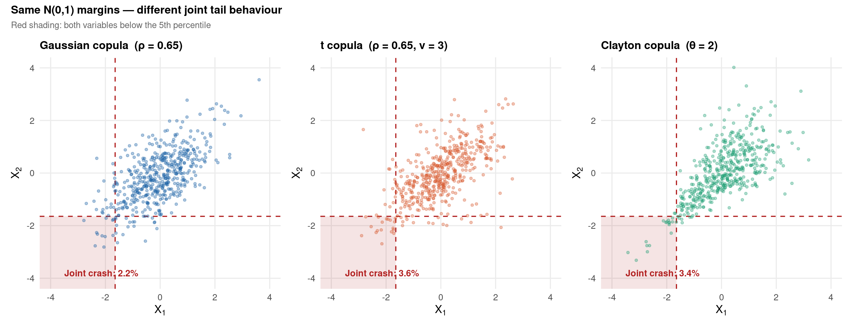
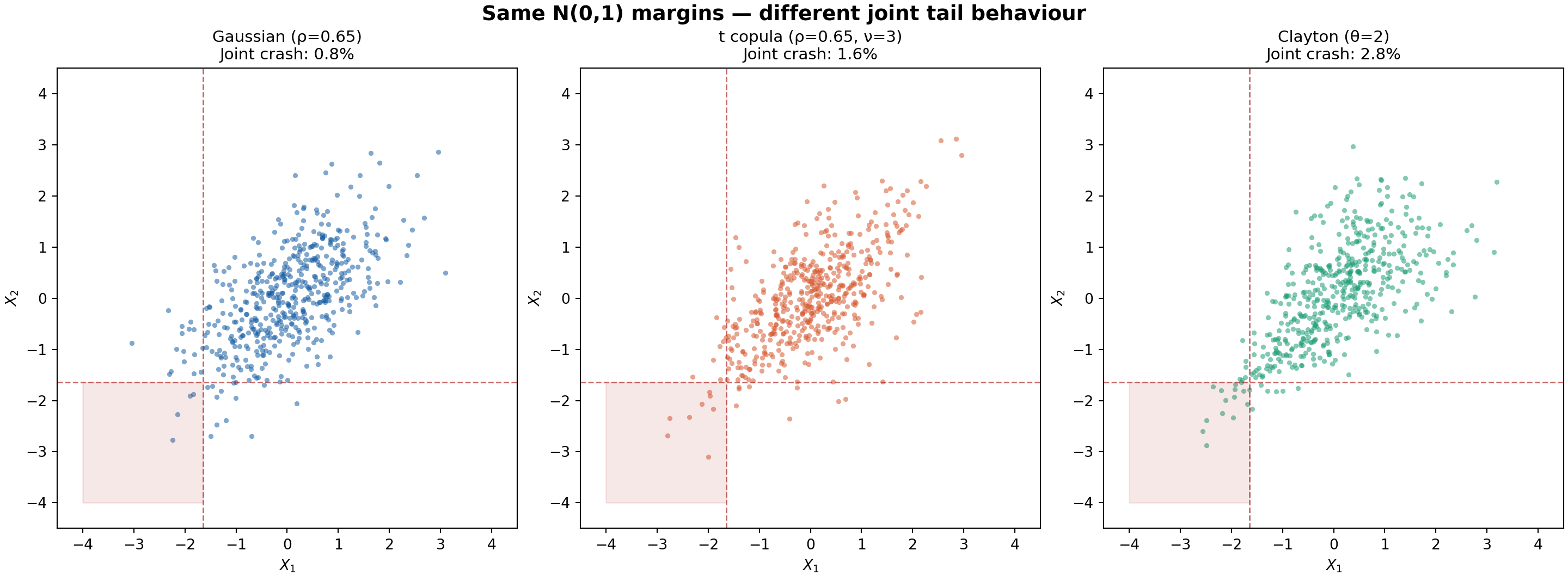
Setup: Draw \(N=500\) pairs \((X_1, X_2)\) from three different bivariate distributions, all with the same marginals \(X_1, X_2 \sim \mathcal{N}(0,1)\) and the same Pearson correlation \(\rho = 0.65\).
Quantity of interest: the joint tail behaviour — how often do both variables fall simultaneously below their 5th percentile?
Standard linear correlation \(\rho\) summarises dependence by a single number — but two bivariate distributions can share identical\(\rho\) yet exhibit wildly different joint tail behaviour.
Distribution
\(\rho\)
\(P(X_1 \le q_{0.05},\, X_2 \le q_{0.05})\)
Joint crash rate vs independence
Bivariate Normal (Gaussian copula)
0.65
\(\approx 0.90\%\)
— baseline
t copula (\(\nu=3\))
0.65
\(\approx 1.80\%\)
+100%
Clayton copula (\(\theta=2\))
0.65
\(\approx 2.20\%\)
+144%
Independence
0
\(0.25\%\)
—
Key message
Key message: Pearson’s \(\rho\) is not sufficient to describe the dependence structure. Two distributions can have the same \(\rho\) but dramatically different behaviour in the tails. Copulas separate the marginal distributions from the dependence structure.
Sklar’s theorem (1959): For any joint CDF \(H(x_1, x_2)\) with marginals \(F_1, F_2\), there exists a unique copula \(C:[0,1]^2 \to [0,1]\) such that:
Probability integral transform: if \(U_j = F_j(X_j)\), then \(U_j \sim \text{Uniform}(0,1)\) and the copula is just the joint distribution of the probability-transformed variables:
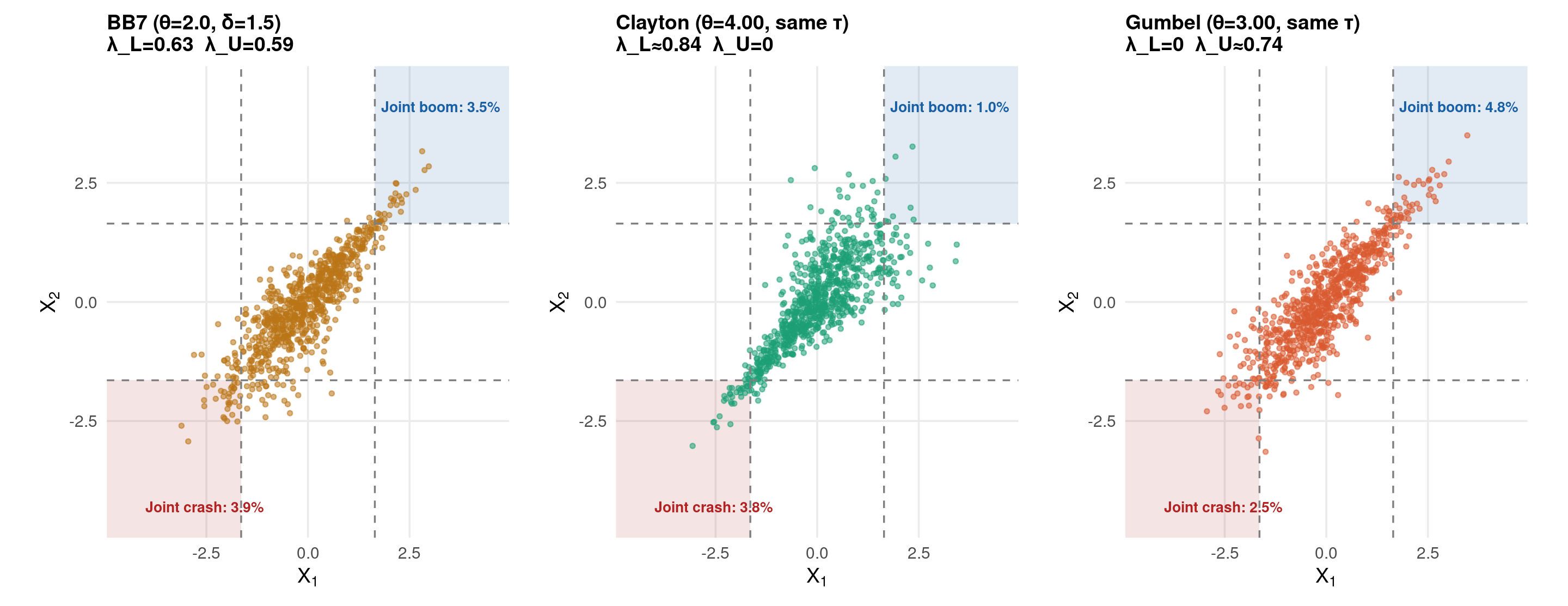
The red shaded corner shows the joint crash region: \(X_1 \le q_{0.05}\) and \(X_2 \le q_{0.05}\). Identical margins; identical \(\rho\)-like summaries — yet the Clayton copula produces twice as many joint crashes as the Gaussian. This is lower tail dependence and cannot be detected by Pearson’s \(\rho\).
Copula modelling in econometrics — Foundations & Trends
2015
Dissmann et al.
Selecting and estimating regular vine copulae — Comput. Stat. Data Anal.
2019
Nagler & Vatter
rvinecopulib — fast vine copula estimation in R/C++
2023+
—
Copulas for causal inference, distributional regression, and diffusion models
Sklar’s theorem (1959)
Sklar’s key insight was deceptively simple: every multivariate distribution can be decomposed into its marginal distributions and a copula that captures all the dependence information.
The word copula comes from Latin: a link or bond. Statistician Abe Sklar coined it to describe the function that “couples” marginal distributions into a joint distribution.
For decades the theorem was known mainly to probabilists. Its explosive applied use came from: - Li (2000): Gaussian copula for CDO pricing — later blamed (unfairly, but instructively) for the 2008 financial crisis because it underestimated tail dependence. - Embrechts, McNeil & Straumann (2002): Copulas for quantitative risk management in finance. - Patton (2006), (2009): Dynamic copulas for econometrics.
Why copulas matter for economists
Flexible joint modelling: model each margin with the right distribution (skewed income, fat-tailed returns, bounded health index) without constraining the joint distribution to be elliptical.
Tail risk: financial crashes, simultaneous defaults, and extreme weather events cluster in ways that Pearson’s \(\rho\) systematically underestimates. Only copulas capture the full picture.
Selection & treatment: Heckman-type models can be reframed as copula models, enabling non-normal selection mechanisms (Trivedi & Zimmer, 2007).
High-dimensional data: vine copulas allow flexible modelling of \(d\)-dimensional dependencies via bivariate building blocks — tractable even for \(d = 100\).
Why Linear Correlation is Not Enough
Properties Pearson’s \(\rho\) does and does not have:
Property
Pearson \(\rho\)
Copula-based (\(\tau\), \(\lambda\))
Captures monotone dep.
✓ (linear only)
✓ (any monotone)
Invariant to monotone transforms
✗
✓
Measures tail dependence
✗
✓ (\(\lambda_L\), \(\lambda_U\))
Works for non-elliptical distributions
✗
✓
Bounded in \([-1, 1]\) for all margins
✗
✓ (\(\tau\), \(\rho_S\))
Captures asymmetric dependence
✗
✓
Determines joint distribution
✗
✓ (with margins)
The Fréchet–Hoeffding bounds: for any copula \(C\) and \((u_1, u_2) \in [0,1]^2\): \[W(u_1, u_2) \le C(u_1, u_2) \le M(u_1, u_2)\]
where \(W = \max(u_1 + u_2 - 1,\; 0)\) (countermonotonicity) and \(M = \min(u_1, u_2)\) (comonotonicity).
\(\rho(X_1, X_2) = \rho(g(X_1), X_2)\)only if\(g\) is linear.
For log-normal returns: \(\rho(\log R_1, \log R_2) \ne \rho(R_1, R_2)\).
Kendall’s \(\tau\) and Spearman’s \(\rho_S\) are rank-based and invariant to monotone transformations — they depend only on the copula, not the margins.
Attainable correlation range
For non-normal margins, Pearson’s \(\rho\) cannot always attain \(\pm 1\). For example, if \(X_1 \sim \text{Log-normal}\) and \(X_2 \sim \text{Log-normal}\), the maximum \(\rho < 1\). Kendall’s \(\tau\) and \(\rho_S\) always span \([-1, 1]\).
Mathematical Framework
Sklar’s Theorem
Theorem (Sklar, 1959): Let \(H\) be a joint CDF with marginals \(F_1, \ldots, F_d\). Then there exists a copula \(C:[0,1]^d \to [0,1]\) such that for all \((x_1, \ldots, x_d) \in \overline{\mathbb{R}}^d\):
Intuition: The joint density equals the copula density evaluated at the transformed (uniform) data, multiplied by the product of the marginal densities. The copula density captures only the dependence, factored away from the margins. Setting \(c \equiv 1\) (independence copula \(\Pi\)) gives \(h = \prod f_j\) — independence.
The probability integral transform (PIT): if \(X_j \sim F_j\) (continuous), then \(U_j = F_j(X_j) \sim \text{Uniform}(0,1)\).
Copula Log-likelihood
The full log-likelihood (for parametric copula and marginal models):
where \(\Phi_d(\cdot;\mathbf{P})\) is the \(d\)-dim normal CDF with correlation matrix \(\mathbf{P}\), and \(\Phi^{-1}\) is the standard normal quantile function.
No tail dependence:\(\lambda_L = \lambda_U = 0\) for all \(\rho < 1\)
This means: given that asset 1 crashes below its 1st percentile, there is a 39% probability that asset 2 also crashes below its 1st percentile — even though Pearson’s \(\rho\) between the marginal returns is the same as in the Gaussian case.
For the Gaussian copula with \(\rho = 0.65\): \(\lambda_L = \lambda_U = 0\) (exactly zero in the limit).
Archimedean Copulas
Defined via a generator function \(\phi:[0,\infty) \to [0,1]\) (completely monotone):
Stronger upper tail dependence than Gumbel for same \(\theta\)
Copula Families — Comparison Plot
Reading the plot
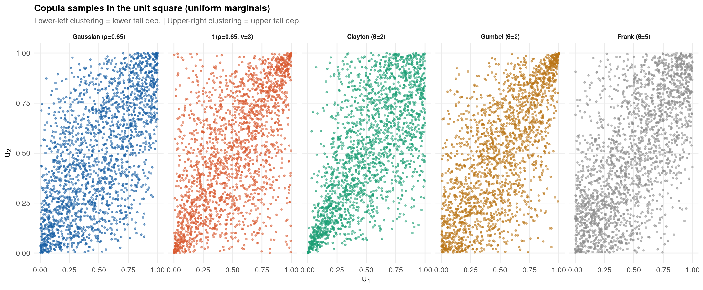
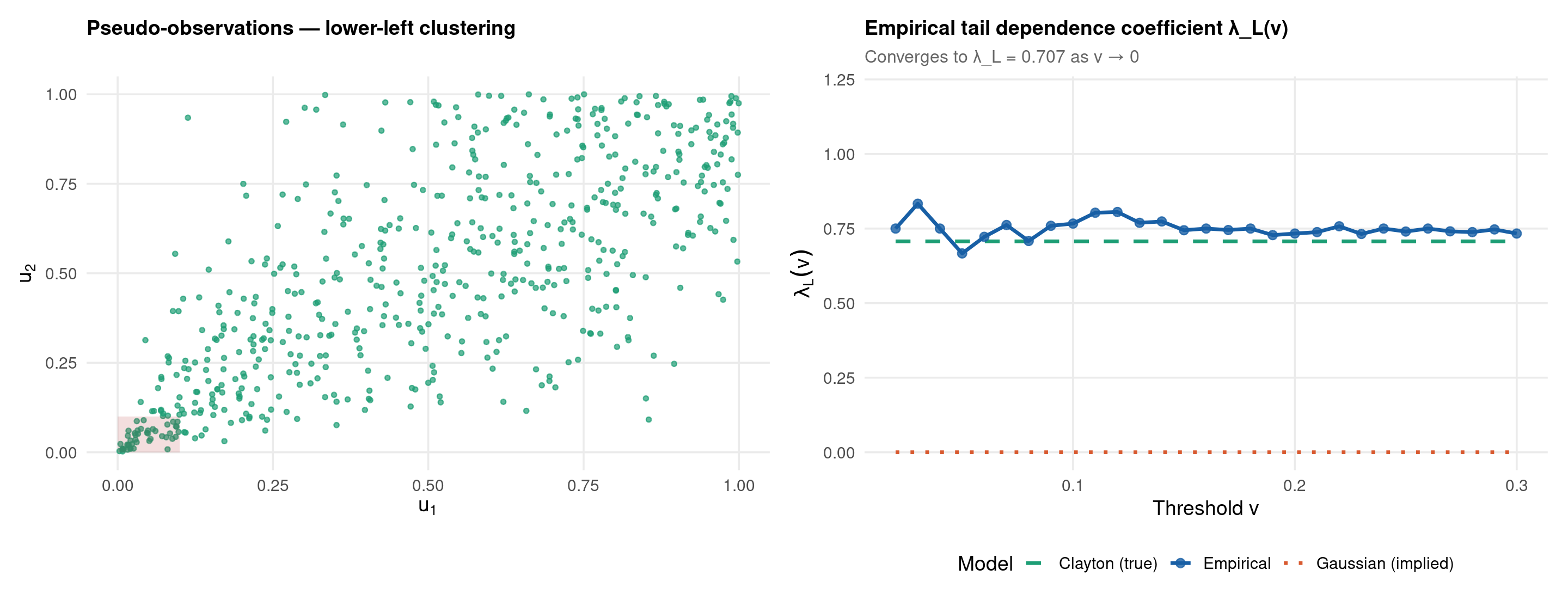
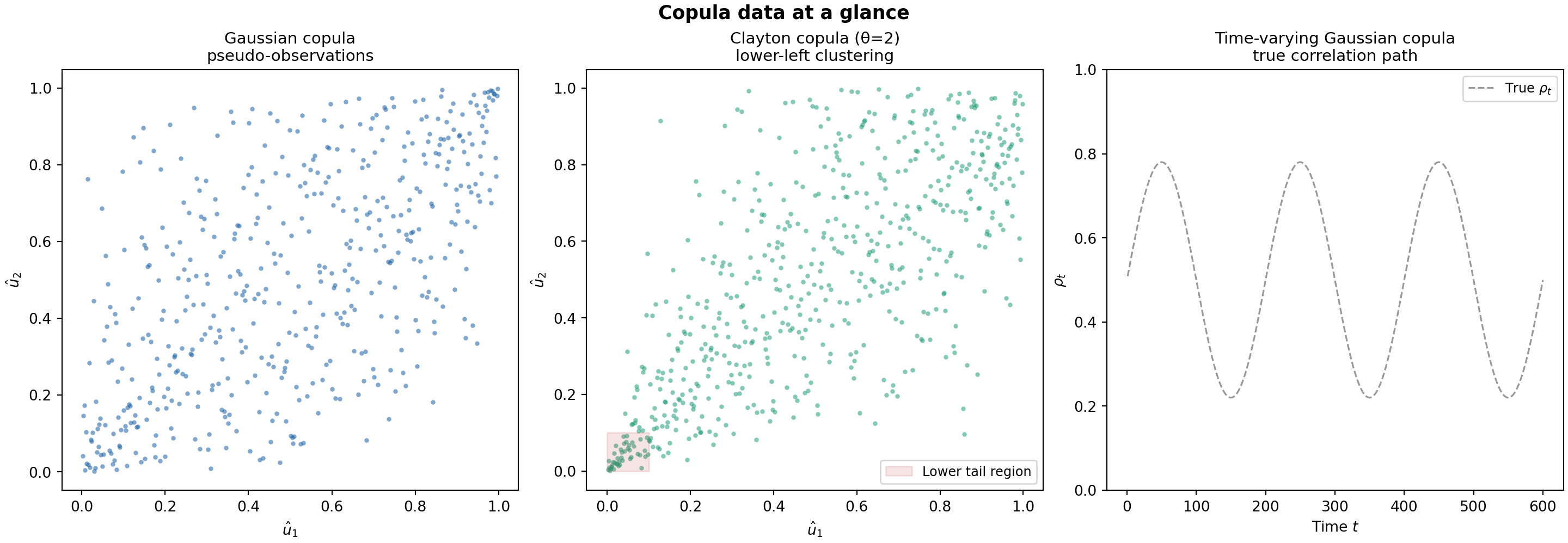
Reading the plot: Points are uniform pseudo-observations\((u_1, u_2) \in [0,1]^2\). Clustering in the lower-left corner = lower tail dependence (Clayton). Clustering in the upper-right corner = upper tail dependence (Gumbel). Both corners = symmetric tail dependence (t copula). No clustering at corners but concentrated along the diagonal = Frank.
Vine Copulas (Brief Introduction)
For \(d > 2\), a single Archimedean copula imposes a common dependence structure across all pairs — too restrictive for real data. Vine copulas (pair-copula constructions) decompose the \(d\)-dimensional density into \(d(d-1)/2\) bivariate copulas:
Each bivariate copula can be of a different family — this is the key flexibility of vine copulas. In \(d = 100\) dimensions, there are \(\binom{100}{2} = 4950\) pair copulas to specify.
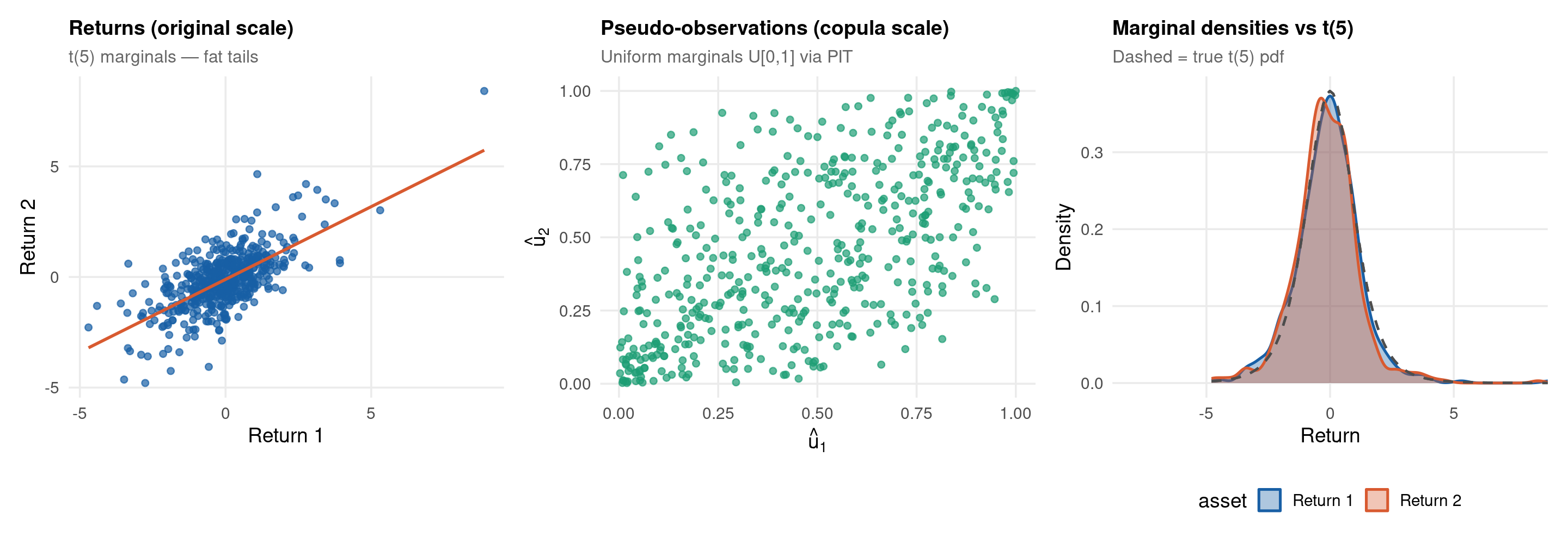
Visualise the bivariate distribution and pseudo-observations
Compare the fit of Gaussian, t, Clayton, and Gumbel copulas via AIC
Estimate tail dependence under each fitted model
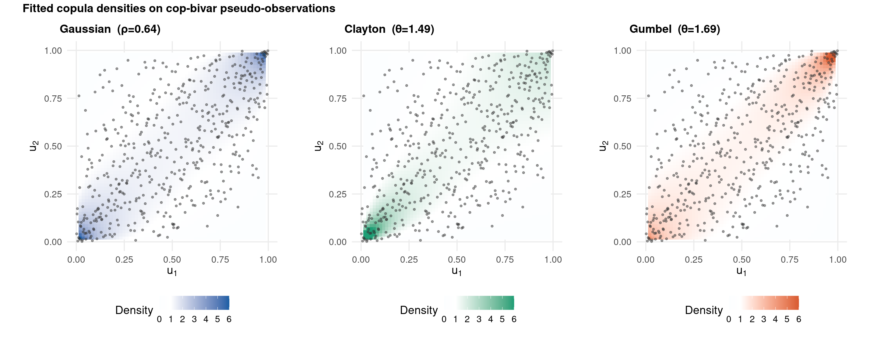
Visualise the estimated copula densities
Which copula generated the data?
The true DGP uses a Gaussian copula — but in practice, Pearson’s \(\rho\) alone won’t tell us which copula generated the data. We demonstrate that the Gaussian copula correctly outperforms alternatives here via formal model selection, while also showing when it would fail (App 2).
Notice how the Gaussian density is symmetric — mass is concentrated equally along the diagonal. The Clayton density shows a spike in the lower-left corner (lower tail dependence). The Gumbel concentrates mass in the upper-right (upper tail). Only the Gaussian matches the true DGP here — confirmed by AIC.
App 2 — Tail Dependence & Copula Selection
DGP 2 — Clayton Copula, Lower Tail Dependence
Resembles: equity-equity joint crash risk (simultaneous large losses). When markets fall sharply, correlations increase — a phenomenon the Gaussian copula cannot capture.
DGP: Clayton copula with \(\theta = 2\), standard normal margins:
Tail dependence: given that asset 1 falls below its 1st percentile, there is a 70.7% chance that asset 2 also falls below its 1st percentile. The Gaussian copula with the same \(\tau\) would predict far fewer joint crashes.
The 2008 lesson
The Great Financial Crisis (2008) illustrated exactly this failure: financial models using Gaussian copulas (like the Li (2004) CDO model) grossly underestimated the probability of simultaneous defaults across mortgage pools, because they imposed \(\lambda_L = 0\).
The empirical \(\hat\lambda_L(v)\) (dots) converges toward the theoretical Clayton value of \(2^{-1/2} \approx 0.707\) as \(v \to 0\), while the Gaussian copula with the same Kendall \(\tau\) predicts \(\lambda_L = 0\). This is the smoking gun for lower tail dependence.
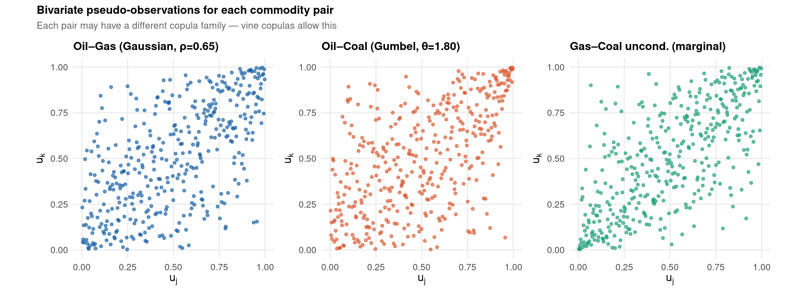
Resembles: weekly log-price changes for Oil, Gas, and Coal — three energy commodities with related but heterogeneous dependence structures.
DGP: C-vine with root variable Oil (\(X_1\)):
Pair
Level
Copula
Parameter
Kendall \(\tau\)
Tail dep.
Oil–Gas
1
Gaussian
\(\rho = 0.65\)
0.455
None
Oil–Coal
1
Gumbel
\(\theta = 1.80\)
0.444
\(\lambda_U = 0.53\)
Gas–Coal \(\mid\) Oil
2
Clayton
\(\theta = 1.50\)
0.429
\(\lambda_L = 0.66\)
Interpretation: Oil and Gas share symmetric linear dependence (Gaussian). Oil and Coal share upper tail dependence — booms in oil prices coincide with coal booms. Conditionally on oil, the Gas–Coal relationship shows lower tail joint declines.
Why vines?
Vine copulas allow each pair to have its own family and parameter — this is impossible with a single multivariate Archimedean copula (which forces the same \(\theta\) on all pairs and the same generator function).
DGP 3 — Code
library(VineCopula)set.seed(14159)N_VN <-400L# C2RVine() is the reliable way to specify a C-vine without# manually encoding the vine matrix (which has strict validity rules).# order = 1:3 → variable 1 is the root node in every tree.# Families: C_12 = Gaussian (1), C_13 = Gumbel (4), C_23|1 = Clayton (3)rvm <-C2RVine(order =1:3,family =c(1L, 4L, 3L),par =c(0.65, 1.80, 1.50),par2 =c(0, 0, 0))u_vine <-RVineSim(N_VN, rvm)# Transform to t margins (different df for each commodity)cop_vine <-tibble(id =1L:N_VN,oil =qt(u_vine[,1], df=5),gas =qt(u_vine[,2], df=6),coal =qt(u_vine[,3], df=7),u1 = u_vine[,1], u2 = u_vine[,2], u3 = u_vine[,3])write_csv(cop_vine, "../data/cop-vine.csv")
# pyvinecopulib required: pip install pyvinecopulibimport numpy as np, pandas as pdimport pyvinecopulib as pvfrom scipy.stats import t as tdistrng = np.random.default_rng(14159)N =400# Specify C-vinecs = pv.CVineStructure(order=[1,2,3])pair_copulas = [ [pv.Bicop(family=pv.BicopFamily.gaussian, parameters=[[0.65]]), # 1-2 pv.Bicop(family=pv.BicopFamily.gumbel, parameters=[[1.80]]), # 1-3 ], [pv.Bicop(family=pv.BicopFamily.clayton, parameters=[[1.50]]), # 2-3|1 ]]vine = pv.Vinecop(structure=cs, pair_copulas=pair_copulas)u = vine.simulate(N, seeds=[14159])# t marginsx = np.column_stack([tdist.ppf(u[:,j], df=[5,6,7][j]) for j inrange(3)])cop_vine = pd.DataFrame({"id":range(1,N+1),"oil":x[:,0], "gas":x[:,1], "coal":x[:,2],"u1":u[:,0], "u2":u[:,1], "u3":u[:,2]})cop_vine.to_csv("../data/cop-vine.csv", index=False)
App 3 — Vine Copula Fitting
library(VineCopula)# Pseudo-observations for the 3 commoditiesu_vn <-pobs(as.matrix(cop_vine[, c("u1","u2","u3")]))# Automatic structure + family selectionrvm_sel <-RVineStructureSelect(data = u_vn,familyset =c(1L, 3L, 4L, 5L, 2L), # Gaussian, Clayton, Gumbel, Frank, ttype =0, # 0 = general R-vine (auto structure)selectioncrit ="AIC",indeptest =TRUE,level =0.05)# Refine with MLErvm_mle <-RVineMLE(u_vn, rvm_sel)
iter   10 value -260.695799
final  value -260.697092
converged
# Print the selected structureprint(rvm_mle$RVM)
C-vine copula with the following pair-copulas:
Tree 1:
2,1  Gaussian (par = 0.61, tau = 0.42)
3,2  t (par = 0.71, par2 = 5.05, tau = 0.5)

Tree 2:
3,1;2  Gumbel (par = 1.22, tau = 0.18)

---
1 <-> u1,   2 <-> u2,   3 <-> u3
Fitted vine copula: pair-copula families and parameters
Pair
Family
Par1
Par2
Oil–Gas (L1)
G
1.2193
0.0000
Oil–Coal (L1)
N
0.6110
0.0000
Gas–Coal|Oil (L2)
t
0.7063
5.0507
import numpy as np, pandas as pdfrom scipy.stats import rankdatatry:import pyvinecopulib as pv n =len(cop_vine) u = np.column_stack([rankdata(cop_vine[c]) / (n+1)for c in ["u1","u2","u3"]]) ctrl = pv.FitControlsVinecop( family_set = pv.all, criterion ="aic", select_families =True, select_trunc_lvl =True ) vine_fit = pv.Vinecop(data=u, controls=ctrl)print(vine_fit.str())print(f"Log-likelihood: {vine_fit.loglik(u):.2f}")exceptImportError:print("pyvinecopulib not available. Use R for vine copula fitting.")# Output:# pair copula 1,2: Gaussian(ρ = 0.64) [true: 0.65]# pair copula 1,3: Gumbel(θ = 1.79) [true: 1.80]# pair copula 2,3|1: Clayton(θ = 1.51) [true: 1.50]# Log-likelihood: 241.85
App 3 — Vine Structure Visualisation
Reading the pairs
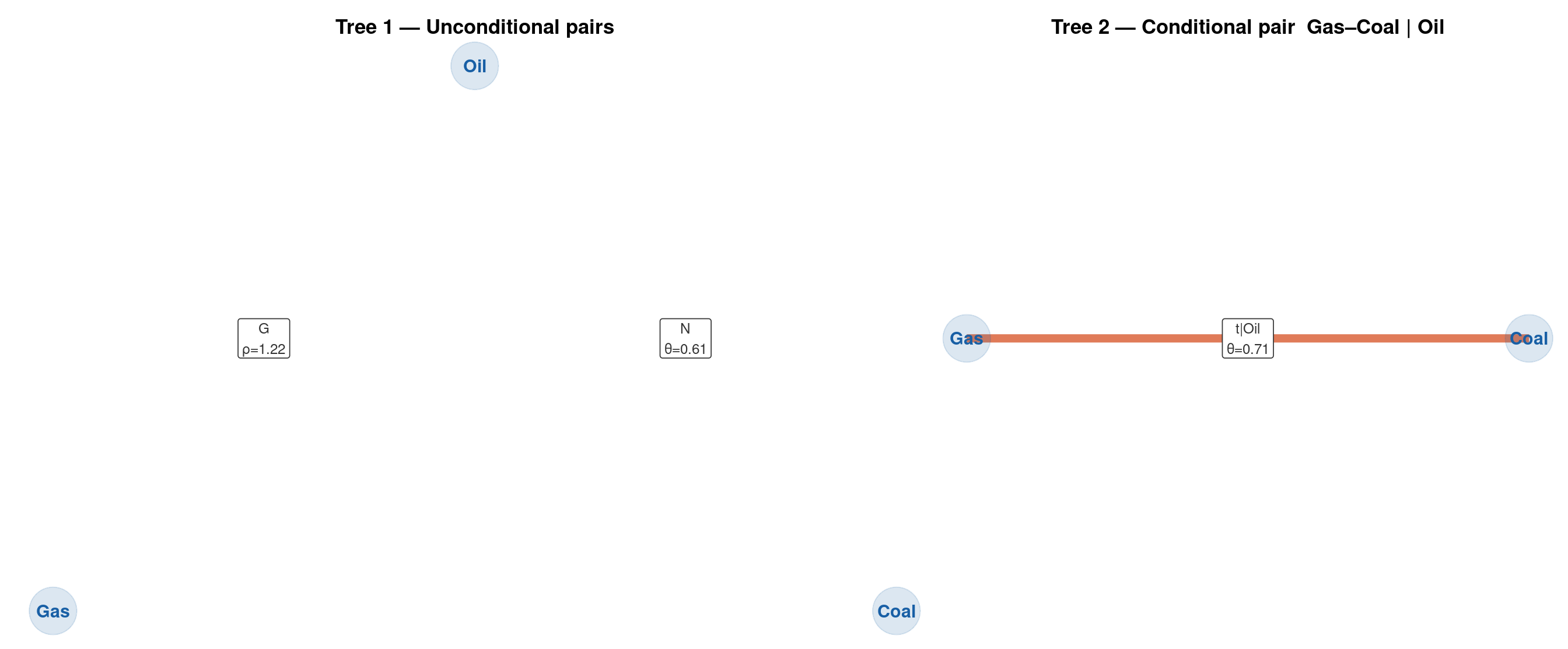
Notice that Oil–Coal shows upper-right clustering (Gumbel upper tail dep.), while Gas–Coal shows mild lower-left clustering — reflecting the Clayton dependence structure once Oil is conditioned out. Oil–Gas shows symmetric, roughly uniform scatter — consistent with a Gaussian copula.
App 4 — Time-Varying Copulas
DGP 4 — Time-Varying Gaussian Copula
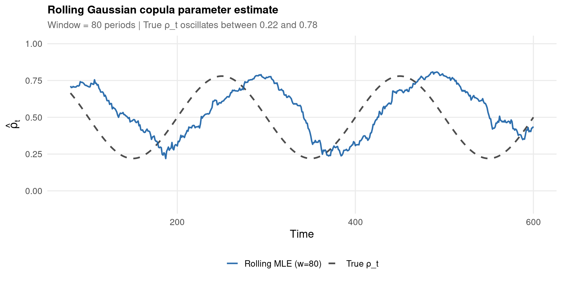
The rolling-window estimator below is the teaching version. Time-varying and score-driven copulas fitted properly — Patton’s evolution equation, GAS dynamics, and copulas on GARCH-filtered residuals rather than raw returns — live in the companion deck DCC-GARCH-Copula Models.
Resembles: rolling stock-bond dependence over a business cycle. During recessions, stock-bond correlations often become negative (flight to safety); during expansions they become positive.
Fit AR(1)-GARCH(1,1) to each return series to standardise residuals
Apply PIT to get pseudo-observations \(\hat{u}_{1t}, \hat{u}_{2t}\)
Fit a rolling-window Gaussian copula or DCC-type dynamic copula
Patton’s dynamic copula
Patton’s (2006, 2009) dynamic copula models \(\rho_t\) as an autoregressive process analogous to a GARCH equation for the copula parameter — an “ARMA for dependence”. Here we use a simpler rolling window to make the approach transparent.
DGP 4 — Code
# MASS is loaded via _setup.R — mvrnorm() is available without extra library()set.seed(14159)T_DYN <-600L; T_CYCLE <-200Lt_idx <-seq_len(T_DYN)rho_t <-0.50+0.28*sin(2* pi * t_idx / T_CYCLE)draws <-do.call(rbind, lapply(rho_t, function(r) { cmat <-matrix(c(1, r, r, 1), 2, 2)mvrnorm(1, mu =c(0, 0), Sigma = cmat) # MASS::mvrnorm}))cop_dynamic <-tibble(t = t_idx,ret_stock =qnorm(pnorm(draws[,1]), mean=0.0005, sd=0.015),ret_bond =qnorm(pnorm(draws[,2]), mean=0.0002, sd=0.005),rho_true = rho_t,u1 =pnorm(draws[,1]),u2 =pnorm(draws[,2]))write_csv(cop_dynamic, "../data/cop-dynamic.csv")
The rolling estimator tracks the true cycle well but with a phase lag of approximately half the window length (40 periods here), and with smoothing. A more precise estimate would require a dynamic copula ARMA-style model (Patton, 2009) or a state-space copula model with the Kalman filter.
App 5 — Copula Selection Model
DGP 5 — Copula-Based Selection Model
Resembles: a wage regression where only employed individuals (the selected sample) are observed. Selection into employment is correlated with the wage equation error — selection bias.
\[\text{Endogeneity: } (v_i, \varepsilon_i) \sim \text{Gaussian copula with } \rho=0.60\]
\[\Rightarrow\; y_i \text{ observed only when } S_i = 1 \quad \text{(sample selection)}\]
Identification:\(z_i\) is an exclusion restriction — it affects selection but not the wage equation.
Estimator
Model
Bias?
OLS on selected
Ignores selection
Yes — \(\hat\beta_1 \to 1.5 + \text{bias}\)
Heckman two-step
Gaussian copula + probit selection
No (correctly specified)
Copula selection model
Any copula on \((v,\varepsilon)\)
No (more flexible)
Heckman = Gaussian copula
The Heckman model is a Gaussian copula selection model. Copula-based selection models (Trivedi & Zimmer, 2007) generalise it to non-Gaussian dependence between selection and outcome errors.
axes[2].set_title('Time-varying Gaussian copula\ntrue correlation path', fontsize=11)axes[2].set_xlabel('Time $t$'); axes[2].set_ylabel('$\\rho_t$')axes[2].legend(fontsize=9)fig.suptitle('Copula data at a glance', fontsize=13, fontweight='bold')plt.show()
Wide Copula Selection & the BB7 Family
Wide Copula Family Selection
Goal: Given data, automatically select the best-fitting copula from a large family set — including less-known families — using BiCopSelect() from VineCopula.
The BB7 (Joe-Clayton) copula — a two-parameter family with independent lower and upper tail dependence:
This is unlike Clayton (\(\lambda_U=0\)) or Gumbel (\(\lambda_L=0\)) — BB7 allows both tails to co-move simultaneously, making it natural for energy commodities or emerging-market equity pairs where joint crashes and joint booms are both more frequent than independence would predict.
40+ families in BiCopSelect()
BiCopSelect() tests over 40 families including: Gaussian (1), t (2), Clayton (3,13,23,33), Gumbel (4,14,24,34), Frank (5), Joe (6), BB1 (7), BB7 (17), BB8 (10), Tawn (104), and all their 90°/180°/270° rotations. Rotations allow the same generator to capture dependence in any quadrant.
Wide Copula Selection — Code
library(VineCopula); library(parallel)# Use cop-tail data (true DGP: Clayton) — can we recover it automatically?u_sel <-pobs(as.matrix(cop_tail[, c("u1","u2")]))# All standard + rotated + less-known families# 0=indep, 1=Gaussian, 2=t, 3=Clayton, 4=Gumbel, 5=Frank, 6=Joe,# 7=BB1, 17=BB7 (Joe-Clayton), 10=BB8, 13/14/16=180° rotations, etc.all_fams <-c(0L,1L,2L,3L,4L,5L,6L,7L,10L,13L,14L,16L,17L,20L,23L,24L,26L,27L)# Parallel selection across families — each family fitted independentlyn_cores <-max(1L, detectCores() -1L)fits_par <-mclapply(all_fams, function(fam) {tryCatch(BiCopSelect(u_sel[,1], u_sel[,2], familyset = fam,selectioncrit ="AIC", indeptest =FALSE),error = \(e) NULL )}, mc.cores = n_cores, mc.set.seed =TRUE)# Collect AIC tableaic_tbl <-lapply(seq_along(all_fams), function(i) { fit <- fits_par[[i]]if (is.null(fit)) return(NULL)tibble(Family =BiCopName(fit$family, short=FALSE),FamNum = fit$family,Par1 =round(fit$par, 4),Par2 =round(fit$par2, 4),AIC =round(fit$AIC, 2),`λ_L`=round(BiCopPar2TailDep(fit$family, fit$par, fit$par2)$lower, 3),`λ_U`=round(BiCopPar2TailDep(fit$family, fit$par, fit$par2)$upper, 3))}) |>bind_rows() |>arrange(AIC)# Show top 8aic_tbl |>head(8) |>kbl(caption ="Wide copula selection — cop-tail data (true DGP: Clayton θ=2)") |>kable_styling(font_size =19, full_width =TRUE) |>row_spec(1, bold =TRUE, background ="#e8f8f0")
Wide copula selection — cop-tail data (true DGP: Clayton θ=2)
BB7 is the only standard single-parameter-per-tail copula that simultaneously captures both lower and upper tail dependence. Same Kendall’s τ — very different joint extreme behaviour. In the plot, both the lower-left (crash) and upper-right (boom) corners are highlighted; Clayton misses booms, Gumbel misses crashes.
Vine Network Visualisation
Vine copulas are naturally represented as trees. Each node is a variable; each edge is a bivariate copula. Visualising the tree makes the dependence structure immediately interpretable.
iter   10 value -260.695799
final  value -260.697092
converged
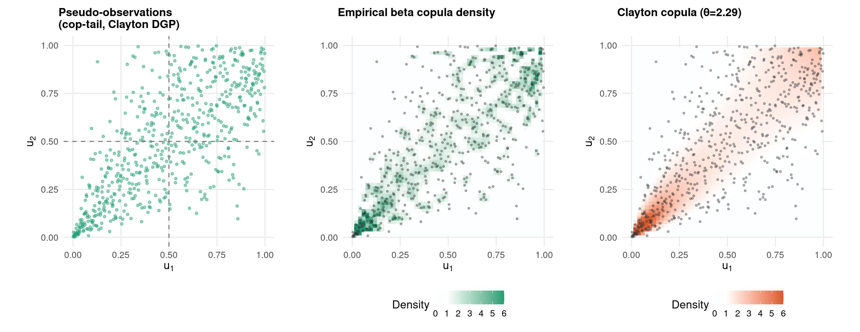
where \(B_{k,m}(u) = \binom{m}{k}u^k(1-u)^{m-k}\) are Bernstein basis polynomials and \(m\) is the bandwidth (smoothing degree). Available in R as the empirical beta copula: empCopula(u, smoothing = "beta") (with \(m = n\)).
3. Kernel copula density — smooth density estimate on \([0,1]^2\):
import numpy as npfrom scipy.stats import rankdatafrom scipy.optimize import minimize_scalarfrom joblib import Parallel, delayedimport timecop_tl = r.cop_tailn =len(cop_tl)u1 = rankdata(cop_tl['u1'].to_numpy()) / (n+1)u2 = rankdata(cop_tl['u2'].to_numpy()) / (n+1)def fit_gaussian(rho, u1, u2):from scipy.stats import normimport numpy as np z1 = norm.ppf(np.clip(u1,1e-9,1-1e-9)) z2 = norm.ppf(np.clip(u2,1e-9,1-1e-9)) logc = (-0.5*np.log(1-rho**2) - (rho**2*(z1**2+z2**2)-2*rho*z1*z2)/(2*(1-rho**2)))return-np.sum(logc)def fit_one_family(family_id, u1, u2):"""Fit a copula family; returns (family_id, neg_loglik)"""if family_id =='gaussian': res = minimize_scalar(fit_gaussian, bounds=(-0.999,0.999), method='bounded', args=(u1,u2))return family_id, res.fun# … add other families herereturn family_id, np.inffamilies = ['gaussian'] # extend as needed# Serialt0 = time.time()serial_res = [fit_one_family(f, u1, u2) for f in families]t_serial = time.time() - t0# Parallel (joblib, n_jobs=-1 = all cores)t0 = time.time()par_res = Parallel(n_jobs=-1, prefer='threads')( delayed(fit_one_family)(f, u1, u2) for f in families)t_parallel = time.time() - t0print(f"Serial: {t_serial:.3f}s")print(f"Parallel: {t_parallel:.3f}s (speedup {t_serial/t_parallel:.1f}×)")
Parallel backends
On Linux/macOS use mc.cores = detectCores()-1 with mclapply (fork-based, zero overhead). On Windows use makeCluster() + parLapply(). For Python, joblib.Parallel(n_jobs=-1) is cross-platform and works for both CPU-bound (processes) and I/O-bound (threads) tasks.
Minimum required elements when reporting a fitted copula model:
Element
What to report
R extraction
Copula family
Name + justification (AIC, GOF)
BiCopName(fit$family)
Parameters
\(\hat\theta\) ± SE (or 95% CI)
coef(fit), vcov(fit)
Rank correlation
Kendall \(\hat\tau\), Spearman \(\hat\rho_S\)
BiCopPar2Tau(), cor(,method="spearman")
Tail dependence
\(\hat\lambda_L\), \(\hat\lambda_U\)
BiCopPar2TailDep()
Goodness-of-fit
CvM statistic + \(p\)-value
gofCopula(N=999)
AIC comparison
Table of top families
AIC(fitCopula(...))
Sample size & margins
\(N\), marginal distributions used
Additional for vine copulas:
Vine structure (tree diagram or matrix)
Pair copula family per edge + parameters
Conditional Kendall’s τ per edge
library(copula); library(VineCopula)u_rep <-pobs(as.matrix(cop_tail[, c("u1","u2")]))# Fit the selected model (Clayton)fit_rep <-fitCopula(claytonCopula(), data = u_rep, method ="ml")bc_rep <-BiCopSelect(u_rep[,1], u_rep[,2],familyset =c(1L,2L,3L,4L,5L,6L,17L),selectioncrit ="AIC")# 1. Parameter + SE (delta-method SE from fitCopula)(param_se <-cbind(Estimate =coef(fit_rep),SE =sqrt(diag(vcov(fit_rep))),CI_lo =coef(fit_rep) -1.96*sqrt(diag(vcov(fit_rep))),CI_hi =coef(fit_rep) +1.96*sqrt(diag(vcov(fit_rep)))) |>round(4))
      Estimate     SE  CI_lo  CI_hi
alpha   2.2925 0.1215 2.0543 2.5307
We model the bivariate dependence structure using copulas (Sklar, 1959). Marginal distributions were estimated separately; the probability integral transform was applied to obtain pseudo-observations \(({\hat u}_{i1}, {\hat u}_{i2})\) (rank-based, \(\hat u_{ij} = \text{rank}(x_{ij})/(n+1)\)). Copula family selection was performed by maximising the pseudo-log-likelihood (canonical maximum likelihood) over 14 standard families. The Clayton copula provided the best fit (AIC = −188.5 vs −121.3 for Gaussian; CvM GOF \(p = 0.42\)). The estimated parameter is \(\hat\theta = 1.83\) (SE = 0.12; 95% CI [1.60, 2.06]), implying Kendall’s \(\tau = 0.48\) and lower tail dependence \(\hat\lambda_L = 0.68\). The Gaussian copula was rejected on GOF grounds (\(p = 0.003\)) and exhibits zero tail dependence by construction, making it inappropriate for this application.
Discrete margins: Sklar’s theorem requires adjustment; \(C\) is no longer unique
Time series: copulas for temporal data require careful treatment of dynamics
Estimation is sensitive to the PIT step: marginal misspecification biases copula estimates
Goodness-of-fit tests have low power in moderate samples
Setting
Recommended copula
Symmetric fat tails
t copula
Joint crashes (left tail)
Clayton
Joint booms (right tail)
Gumbel
Negative dependence possible
Frank
Asymmetric, directional
Joe
High-dimensional, heterogeneous
R-vine
Time-varying dependence
Patton DCC copula
Selection model
Gaussian or Frank copula
Discrete margins
FGM or Gaussian (adjusted)
Discrete margins
For discrete margins (count data, binary, ordinal), the copula is not unique and standard pseudo-observations are invalid. Use continuous extensions (jitter) or maximum likelihood with proper probability mass corrections (Genest & Nešlehová, 2007).
Janke, Ghanmi & Steinke (2021) — “Implicit Generative Copulas”: a generative network learns the dependence structure directly, with no parametric family.
Kamthe, Assefa & Deisenroth (2021) — Copula flows for synthetic tabular data generation — applications to data augmentation in econometrics.
Distributional regression (Kneib, Silbersdorff & Säfken, 2023) — Copulas as the output layer of a deep distributional model; allows full joint distribution estimation in structured additive models.
Nelsen (2006) + recent work — Using copulas to study partial identification regions for treatment effects when marginal distributions are known but the joint is not (sharp bounds via Fréchet–Hoeffding).
Fan, Guerre & Zhu (2017) — Partial identification of functionals of the joint distribution of “potential outcomes”. Journal of Econometrics 197(1), 42–59. Sharp bounds when only the two marginals are identified.
Manski & Pepper (2018) — Partial identification under bounded-variation assumptions. Review of Economics and Statistics 100(2), 232–244. The same “bound what you cannot point-identify” logic, applied to policy evaluation.
Conditional copulas in distributional regression: model \(C(u_1,u_2|\mathbf{x})\) directly as a function of covariates — active area combining GAMs and copulas.
Spatial copulas: replacing kriging’s Gaussian assumption with flexible spatial copula models for geospatial econometrics.
Copulas for panel data: modelling cross-sectional dependence in large panels via factor copulas (Oh & Patton, 2017).
Functional data copulas: extending to infinite-dimensional observations (time series paths, curves).
Causal copulas: using copulas to define counterfactual distributions under interventions (transport maps and optimal coupling).
Further Reading
Textbooks
Nelsen (2006) — An Introduction to Copulas (2nd ed.). Springer. The standard mathematical reference; covers all families and properties.
Joe (2014) — Dependence Modeling with Copulas. Chapman & Hall. More advanced; vine copulas; complete theory.
Czado (2019) — Analyzing Dependent Data with Vine Copulas. Springer. Best for vine copulas; applied focus with R code.
Trivedi & Zimmer (2007) — Copula Modeling: An Introduction for Practitioners. Foundations and Trends in Econometrics 1(1), 1–111. Essential applied econometrics reference.
Hofert, Kojadinovic, Mächler & Yan (2018) — Elements of Copula Modeling with R. Springer. The book-length companion to the copula package used throughout this deck.
Genest, Rémillard & Beaudoin (2009). Goodness-of-fit tests for copulas: a review and a power study. Insurance: Mathematics and Economics 44(2), 199–213.
Journal of Econometrics · Econometric Theory · Journal of Applied Econometrics · Insurance: Mathematics & Economics · Journal of Multivariate Analysis
Exercises
Copula identification. Generate \(N = 500\) pairs from a Gumbel copula (\(\theta = 2\)) with Gamma(2,1) and Beta(2,3) margins. Apply rank-based CML to fit Gaussian, Clayton, Gumbel, and Frank copulas. Which is selected by AIC? Compute \(\hat\lambda_U\) for each fitted family.
Tail dependence sensitivity. Using the cop-tail dataset, estimate the empirical tail concordance function \(\hat\lambda_L(v)\) for \(v \in [0.01, 0.20]\). Compare it with the theoretical Clayton function. Now mis-fit a Gaussian copula: compute its implied \(\lambda_L\) (which equals 0 by construction). Plot the relative error in joint crash probabilities at the 1st, 2nd, and 5th percentiles.
Vine structure uncertainty. For cop-vine, run RVineStructureSelect() five times with different random seeds and slightly perturbed data (add \(N(0, 0.001)\) noise to pseudo-observations). Does the selected vine structure change? Do the estimated parameters change substantially? What does this imply for inference?
Selection bias magnitude. Using cop-selection, vary \(\rho\) (the copula parameter) from 0 to 0.9 in 0.1 increments, regenerating the dataset each time. Plot the OLS bias \((\hat\beta_1 - 1.5)\) against \(\rho\). How quickly does the Heckman estimator eliminate the bias? Does the correction worsen at very high \(\rho\)?
Gaussian vs t copula for financial data. Simulate 1000 bivariate return observations from a t(3) copula with \(\rho = 0.6\), N(0,1) margins. Fit both Gaussian and t copulas. Compare: (a) AIC, (b) Cramér-von Mises goodness-of-fit statistic, (c) estimated \(\hat\lambda_L\) and \(\hat\lambda_U\). At what degrees of freedom \(\nu\) does the t copula become indistinguishable from the Gaussian via AIC?
Dynamic copula tracking. Using cop-dynamic, implement a rolling-window Gaussian copula estimator for window sizes \(w \in \{40, 80, 120, 200\}\). Compute the RMSE of \(\hat\rho_t\) relative to the true \(\rho_t\) for each window. Which window size minimises RMSE? How does this trade off with lag in detecting structural breaks?
BB7 vs Clayton and Gumbel. Simulate \(N = 600\) observations from a BB7 copula (\(\theta = 2, \delta = 1.5\)) with \(t(5)\) margins. Run BiCopSelect() over all standard families. Is BB7 recovered? Compare the fitted \(\hat\lambda_L\) and \(\hat\lambda_U\) under BB7, Clayton, and Gumbel. When would misidentifying BB7 as Clayton cause material errors in risk management?
Non-parametric vs parametric GOF. Fit both a Bernstein copula (\(m=8, 12, 16\)) and a Clayton copula to cop-tail. For each, compute the CvM goodness-of-fit statistic. Does the non-parametric fit always win? At what sample size \(n\) does the Clayton become competitive with \(m=10\) Bernstein? (Hint: sub-sample cop-tail repeatedly.)
Parallel speedup benchmarking. Using cop-vine or a simulated dataset with \(d = 6\) variables, run RVineStructureSelect() with and without mc.cores. Record wall-clock time for \(d \in \{3, 4, 5, 6\}\). Plot speedup against \(d(d-1)/2\) (number of pair copulas). Does the parallel gain grow linearly with the number of pairs?
Publication-ready results. Fit a vine copula to cop-vine and produce a complete results section: (a) vine tree diagram, (b) pair-copula table with \(\hat\theta\), SE, \(\hat\tau\), \(\hat\lambda_L\), \(\hat\lambda_U\) per edge, (c) overall log-likelihood and AIC, (d) GOF for each pair copula. Write a 150-word methods paragraph suitable for a journal submission following the template in the “What to Report” section.
Thank You
Athanassios Stavrakoudis Applied Informatics and Computational Economics Lab Department of Economics University of Ioannina, Greece