DCC-GARCH-Copula Models

Dynamic Volatility, Time-Varying Dependence, and Tail Risk
using R, Python & Stata

Athanassios Stavrakoudis

astavrak@uoi.gr

Applied Informatics and Computational Economics Lab

12 May 2026

Outline

• Roadmap
• How the deck is ordered
• Scope

• Part 1 — Motivation & DGP
  stylised facts, the cost of ignoring them, simulation design
• Part 2 — Stage 1: GARCH margins
  sGARCH, GJR, EGARCH, APARCH; leverage, diagnostics, PIT
• Part 3 — Stage 2: MGARCH & DCC
  CCC, DCC, cDCC, ADCC; the constant-correlation test
• Part 4 — Stage 3: Copula on filtered residuals
  static, Patton (2006), GAS; tail dependence paths

• Part 5 — Risk & backtesting
  VaR, ES, Kupiec, Christoffersen, DQ, Fissler–Ziegel
• Part 6 — Portfolio & systemic risk
  hedge ratios, CoVaR, SRISK, connectedness, wider applications
• Part 7 — Modern & high-dimensional
  DCC-MIDAS, shrinkage, factor copulas, vine-GARCH, ML
• Part 8 — Practice & exercises
  reporting checklist, pitfalls, exercises, further reading

Two deliberate departures from the standard order used in this lecture series. Both are choices, not drift.

1. The toy example comes before the literature review. The hook is a bank and an oil major whose correlation runs from \(-0.09\) in January 2007 to \(0.84\) at the COVID crash of March 2020 — a full-sample \(0.481\) describes neither. Nobody cares which papers solved that problem until they have seen it happen. Required Packages still comes first.

2. The tests are distributed, not collected in one section. This deck uses eight of them — ARCH-LM, Ljung–Box, Engle–Ng, Engle–Sheppard, Kupiec, Christoffersen, DQ, Fissler–Ziegel — and each belongs beside the stage it validates. Gathering them into a single block would separate every test from the model it is testing. Each still gets its own theory slide and code slide.

This deck is about dependence that moves with time.

The companion deck Copula Methods in Economics and Econometrics covers the static theory in depth: Sklar’s theorem, the probability integral transform, the family catalogue, Fréchet–Hoeffding bounds, goodness-of-fit, and vine construction. That material is not repeated here beyond a single recap slide in Part 1.

The copula deck asks what shape is the dependence?
This deck asks how does that shape change from day to day, and what does the change cost you in risk capital?

Required Packages

library(rugarch)             # ugarchspec(), ugarchfit(), ugarchroll() — Stage 1
library(rmgarch)             # dccspec(), dccfit(), dccforecast() — Stage 2
library(copula)              # fitCopula(), pobs() — Stage 3
library(VineCopula)          # BiCopSelect(), BiCopPar2TailDep()
library(xts)                 # time-indexed series
library(zoo)                 # rollapply() — rolling correlations
library(PerformanceAnalytics) # VaR(), ES() — risk metric cross-checks
library(fGarch)              # qstd(), rstd() — standardised-t helpers
library(tseries)             # jarque.bera.test()
library(FinTS)               # ArchTest() — Engle's ARCH-LM
library(tidyverse)           # data wrangling & ggplot2
library(png)                 # readPNG() — reload Stata-exported graphs

import numpy as np                     # arrays, linear algebra
import pandas as pd                    # data frames, CSV input
import scipy.stats as st               # distributions, hand-coded MLE
from scipy.optimize import minimize    # QMLE for DCC and copula recursions
from arch import arch_model            # univariate GARCH — Stage 1
from arch.univariate import StudentsT, SkewStudent
import statsmodels.api as sm           # ACF, Ljung-Box, VAR/FEVD, quantile reg
import pyvinecopulib as pv             # vine copulas — Part 7
import matplotlib.pyplot as plt        # all figures

* Nothing to install: every command used here ships with Stata SE.
arch        // univariate GARCH/EGARCH/GJR/APARCH, normal / t / GED
mgarch dcc  // Engle (2002) dynamic conditional correlation
mgarch ccc  // Bollerslev (1990) constant conditional correlation
mgarch vcc  // Tse-Tsui (2002) varying conditional correlation
estat archlm, estat ic     // post-estimation diagnostics
qreg, var, irf             // CoVaR (Part 6), connectedness (Part 6)
ml model                   // hand-coded copula likelihoods (Part 4)

There is no copula package for Stata on SSC. Where a slide needs one, it is hand-coded with ml, and where an estimator has no native counterpart at all the slide says so rather than omitting the tab silently.

Two implementations outside these three languages appear constantly in the literature and are worth knowing by name: Kevin Sheppard’s MFE Toolbox for MATLAB (bashtage.github.io/mfe-toolbox), which is the reference implementation many DCC papers actually used, and EViews, which has DCC-GARCH built in. Neither is used here.

Part 1 — Why Dynamic Dependence?

τὰ θνητὰ τοιαῦτʼ· οὐδὲν ἐν ταὐτῷ μένει.

nothing mortal stays the same

Εὐριπίδης, Ἴων 969

One Number for Correlation — Theory & Math

• Idea
• Math

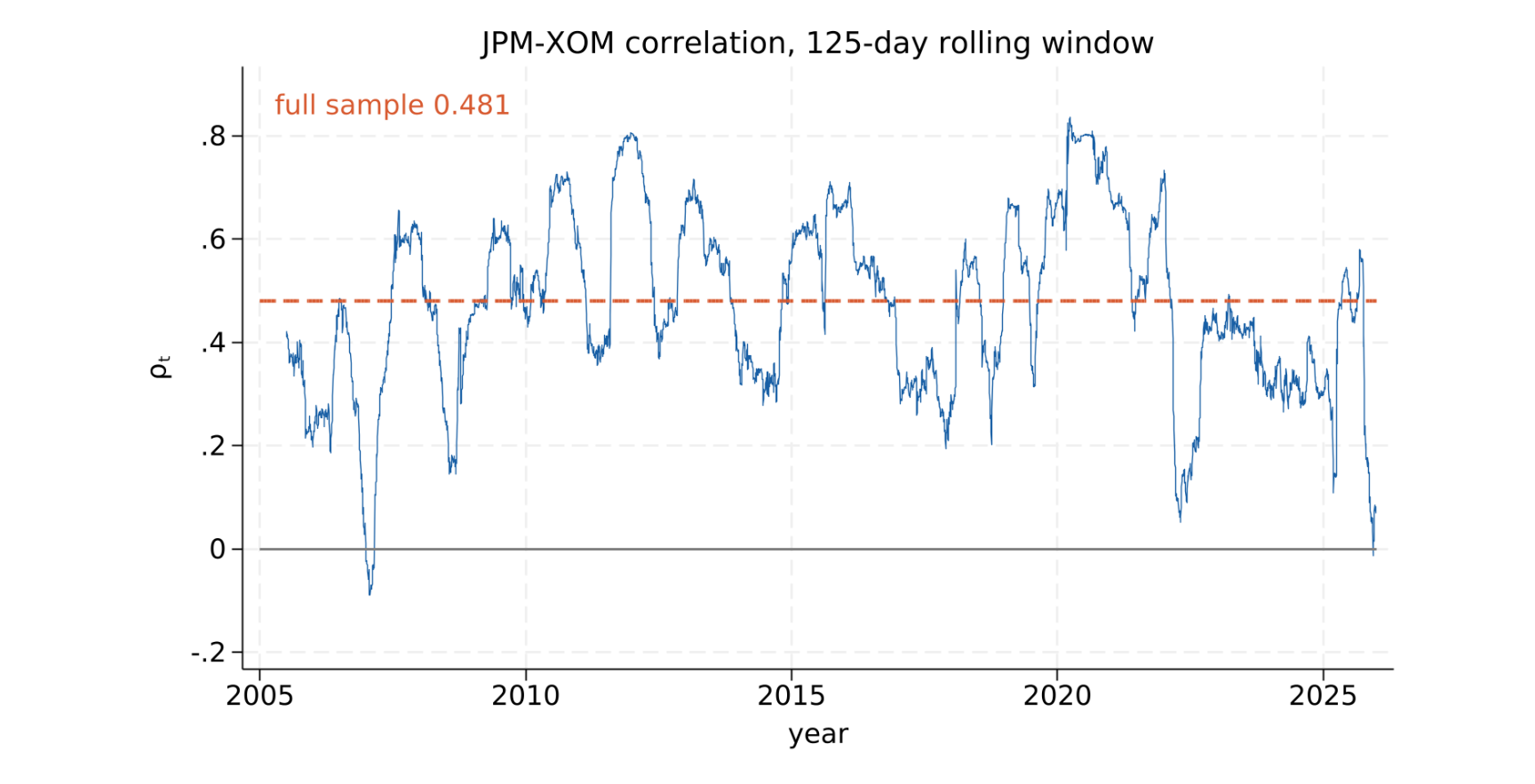
A bank and an oil major: JPMorgan and Exxon Mobil, daily, 2005–2025. Different sectors, different customers, different shocks. Over the full twenty-one years their return correlation is \(0.481\) — moderate, the kind of number that says this pair diversifies.

That number is an average, and it is wrong in both directions.

• Over rolling half-year windows the correlation runs from −0.089 to 0.836
• The minimum is 23 January 2007, the calm before the crisis — the two stocks were effectively unrelated
• The maximum is 30 March 2020, the COVID crash — they had become nearly the same asset
• Yearly averages: \(0.30\) in 2006, \(0.76\) in 2020, back to \(0.34\) by 2025

A portfolio built on \(0.481\) was over-hedged in 2006 and dangerously under-hedged in March 2020. The diversification did not merely weaken — it disappeared in the month it was needed.

The window is a choice, and it matters

A rolling window is the crudest possible estimator of time-varying dependence, and its verdict depends on the width you pick. On this same pair:

• a 125-day window gives -0.089 → 0.836, a swing of 0.93
• a 250-day window gives 0.222 → 0.803, a swing of 0.58

Same data, same pair, same extreme dates — but the wider window erases the episode in which the correlation went to zero. Widen it far enough and you recover the flat line you assumed.

The narrower window buys responsiveness with noise: each estimate rests on 125 observations, so its standard error is roughly \((1-\rho^2)/\sqrt{125} \approx 0.07\) near \(\rho = 0.48\).

Worse, the window is a two-sided assumption: dependence is taken to be exactly constant inside it and unrelated across windows. Neither is plausible.

This is the gap DCC fills. It replaces the arbitrary width with an estimated recursion, so the amount of smoothing is chosen by the data rather than by the analyst. We return to it in Part 3.

Returns are computed as 100 times the log difference of the adjusted close:

\[ r_{i,t} \;=\; 100 \times \bigl(\log P_{i,t} - \log P_{i,t-1}\bigr) \]

The unconditional (full-sample) correlation is the single number:

\[ \hat{\rho}_{ij} \;=\; \frac{\sum_{t=1}^{T} (r_{i,t} - \bar{r}_i)(r_{j,t} - \bar{r}_j)} {\sqrt{\sum_{t=1}^{T} (r_{i,t} - \bar{r}_i)^2}\; \sqrt{\sum_{t=1}^{T} (r_{j,t} - \bar{r}_j)^2}} \]

The rolling correlation applies the same formula to a moving window of width \(w\), ending at \(t\):

\[ \hat{\rho}_{ij,t}^{(w)} \;=\; \frac{\sum_{s=t-w+1}^{t} (r_{i,s} - \bar{r}_{i,t})(r_{j,s} - \bar{r}_{j,t})} {\sqrt{\sum_{s=t-w+1}^{t} (r_{i,s} - \bar{r}_{i,t})^2}\; \sqrt{\sum_{s=t-w+1}^{t} (r_{j,s} - \bar{r}_{j,t})^2}} \]

where \(\bar{r}_{i,t}\) is the mean inside the window. If dependence really were constant, then

\[ \hat{\rho}_{ij,t}^{(w)} \;\longrightarrow\; \rho_{ij} \qquad \text{for every } t \]

and the path would be a flat line plus sampling noise. It is not.

One Number for Correlation — Code

eq <- read.csv("../data/dgcop-equity.csv")

# Full-sample correlation: the single number
rho_full <- cor(eq$jpm, eq$xom)

# Rolling 125-day (half-year) correlation, right-aligned
w <- 125
rho_roll <- rep(NA_real_, nrow(eq))
for (i in w:nrow(eq)) {
  win <- (i - w + 1):i
  rho_roll[i] <- cor(eq$jpm[win], eq$xom[win])
}

cat(sprintf("full sample     : %7.4f\n", rho_full))
cat(sprintf("rolling minimum : %7.4f  (%s)\n",
            min(rho_roll, na.rm = TRUE), eq$date[which.min(rho_roll)]))
cat(sprintf("rolling maximum : %7.4f  (%s)\n",
            max(rho_roll, na.rm = TRUE), eq$date[which.max(rho_roll)]))
cat(sprintf("swing           : %7.4f\n",
            max(rho_roll, na.rm = TRUE) - min(rho_roll, na.rm = TRUE)))

full sample     :  0.4809

rolling minimum : -0.0893  (2007-01-23)

rolling maximum :  0.8356  (2020-03-30)

swing           :  0.9249

import numpy as np
import pandas as pd

eq = pd.read_csv("../data/dgcop-equity.csv")

# Full-sample correlation: the single number
rho_full = eq["jpm"].corr(eq["xom"])

# Rolling 125-day (half-year) correlation, right-aligned
w = 125
rho_roll = eq["jpm"].rolling(w).corr(eq["xom"])

imin = rho_roll.idxmin()
imax = rho_roll.idxmax()

out = (f"full sample     : {rho_full:7.4f}\n"
       f"rolling minimum : {rho_roll.min():7.4f}  ({eq['date'][imin]})\n"
       f"rolling maximum : {rho_roll.max():7.4f}  ({eq['date'][imax]})\n"
       f"swing           : {rho_roll.max() - rho_roll.min():7.4f}")
import sys
nw = sys.stdout.write(out + "\n")

full sample     :  0.4809
rolling minimum : -0.0893  (2007-01-23)
rolling maximum :  0.8356  (2020-03-30)
swing           :  0.9249

sys.stdout.flush()

quietly import delimited "../data/dgcop-equity.csv", clear
tsset t

* Full-sample correlation: the single number
quietly correlate jpm xom
scalar rho_full = r(rho)

* Rolling 125-day (half-year) correlation, right-aligned
quietly gen double rho = .
quietly forvalues i = 125/5281 {
    local lo = `i' - 124
    correlate jpm xom in `lo'/`i'
    replace rho = r(rho) in `i'
}

quietly summarize rho
scalar rmin = r(min)
scalar rmax = r(max)
quietly levelsof date if rho == rmin, local(dmin) clean
quietly levelsof date if rho == rmax, local(dmax) clean

display "full sample     : " %7.4f rho_full
display "rolling minimum : " %7.4f rmin "  (`dmin')"
display "rolling maximum : " %7.4f rmax "  (`dmax')"
display "swing           : " %7.4f rmax - rmin

Time variable: t, 1 to 5281
        Delta: 1 unit










full sample     :  0.4809

rolling minimum : -0.0893  (2007-01-23)

rolling maximum :  0.8356  (2020-03-30)

swing           :  0.9249

One Number for Correlation — Results & Interpretation

• How to run
• Plot
• Reading the output

Window width w. The only free choice, and the one that drives the answer. Half a year (125 trading days) is a common compromise: long enough that the estimate is not pure noise, short enough to resolve a crisis. Report the width; never present a rolling correlation without it.

Alignment. Use right-aligned windows, so the value plotted at \(t\) uses only data up to \(t\). Centre-aligned windows look smoother and leak the future into the present — fatal if the plot is meant to motivate a forecasting model.

The first w-1 values are missing. Not an error. The series begins once a full window exists, which is why the path starts in mid-2005 rather than January.

Language notes. R has no built-in rolling correlation, so the loop is explicit — zoo::rollapply does the same thing. pandas provides .rolling(w).corr() directly. Stata needs the loop with an in range, and tsset must come first.

library(ggplot2)

df <- data.frame(year = eq$year, rho = rho_roll)

ggplot(df) +
  aes(x = year, y = rho) +
  geom_hline(yintercept = 0, colour = "grey55") +
  geom_hline(yintercept = rho_full, colour = "#D85A30",
             linetype = "dashed", linewidth = 0.9) +
  geom_line(colour = "#185FA5", linewidth = 0.6) +
  annotate("text", x = 2007.5, y = 0.86, label = "full sample 0.481",
           colour = "#D85A30", size = 4.2) +
  coord_cartesian(xlim = c(2005, 2026), ylim = c(-0.20, 0.90)) +
  scale_x_continuous(breaks = seq(2005, 2025, 5)) +
  scale_y_continuous(breaks = seq(-0.2, 0.8, 0.2)) +
  labs(x = "year", y = expression(rho[t]),
       title = "JPM-XOM correlation, 125-day rolling window")

import matplotlib.pyplot as plt

fig, ax = plt.subplots(figsize=(9, 4.6))
ax.axhline(0, color="grey")
ax.axhline(rho_full, color="#D85A30", linestyle="--", linewidth=1.4)
ax.plot(eq["year"], rho_roll, color="#185FA5", linewidth=0.9)
ax.text(2007.5, 0.86, "full sample 0.481", color="#D85A30", fontsize=11)
axopts = ax.set(xlim=(2005, 2026), ylim=(-0.20, 0.90),
                xticks=range(2005, 2026, 5),
                yticks=[-0.2, 0.0, 0.2, 0.4, 0.6, 0.8],
                xlabel="year", ylabel=r"$\rho_t$",
                title="JPM-XOM correlation, 125-day rolling window")
plt.tight_layout()
plt.show()

quietly import delimited "../data/dgcop-equity.csv", clear
tsset t
quietly gen double rho = .
quietly forvalues i = 125/5281 {
    local lo = `i' - 124
    correlate jpm xom in `lo'/`i'
    replace rho = r(rho) in `i'
}

twoway (line rho year, lcolor("24 95 165") lwidth(vthin))                     ///
       (function y = 0, range(2005 2026) lcolor(gs8))                         ///
       (function y = 0.4809, range(2005 2026)                                 ///
              lcolor("216 90 48") lpattern(dash) lwidth(medthick)),           ///
    legend(off)                                                               ///
    text(0.86 2007.5 "full sample 0.481", color("216 90 48") size(medsmall))  ///
    xscale(range(2005 2026)) xlabel(2005(5)2025)                              ///
    yscale(range(-0.20 0.90)) ylabel(-0.2(0.2)0.8)                            ///
    xtitle("year") ytitle("{&rho}{sub:t}")                                    ///
    title("JPM-XOM correlation, 125-day rolling window", size(medium))        ///
    graphregion(color(white)) plotregion(color(white))

graph export "../plots/dgcop-p1-roll.png", replace width(1600)

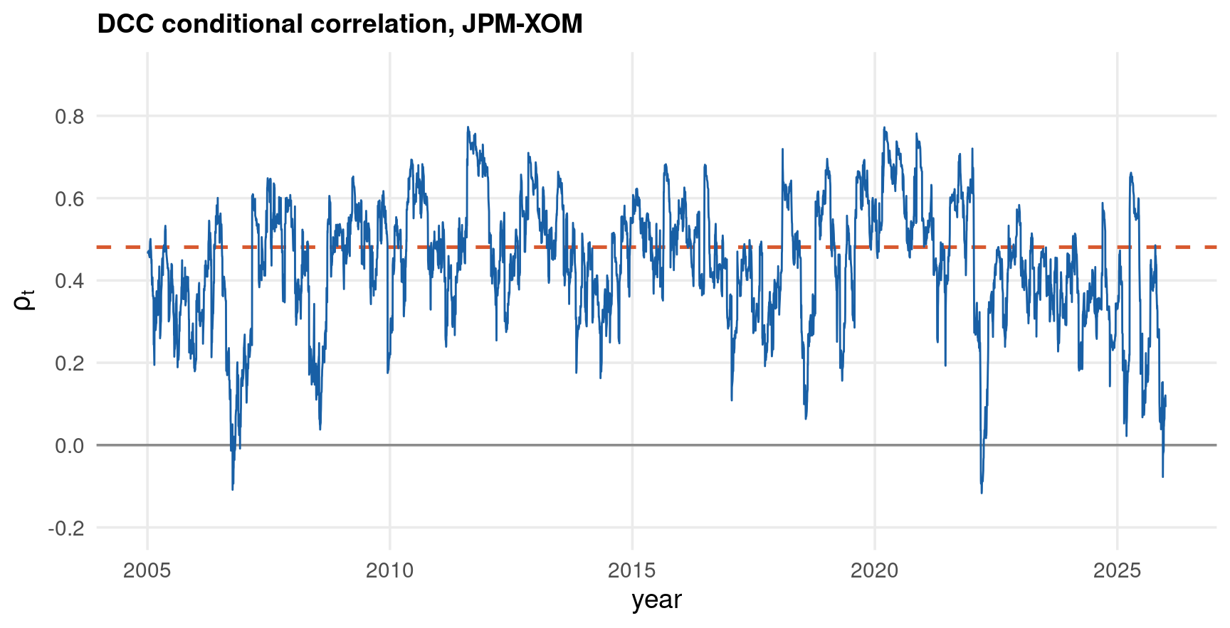
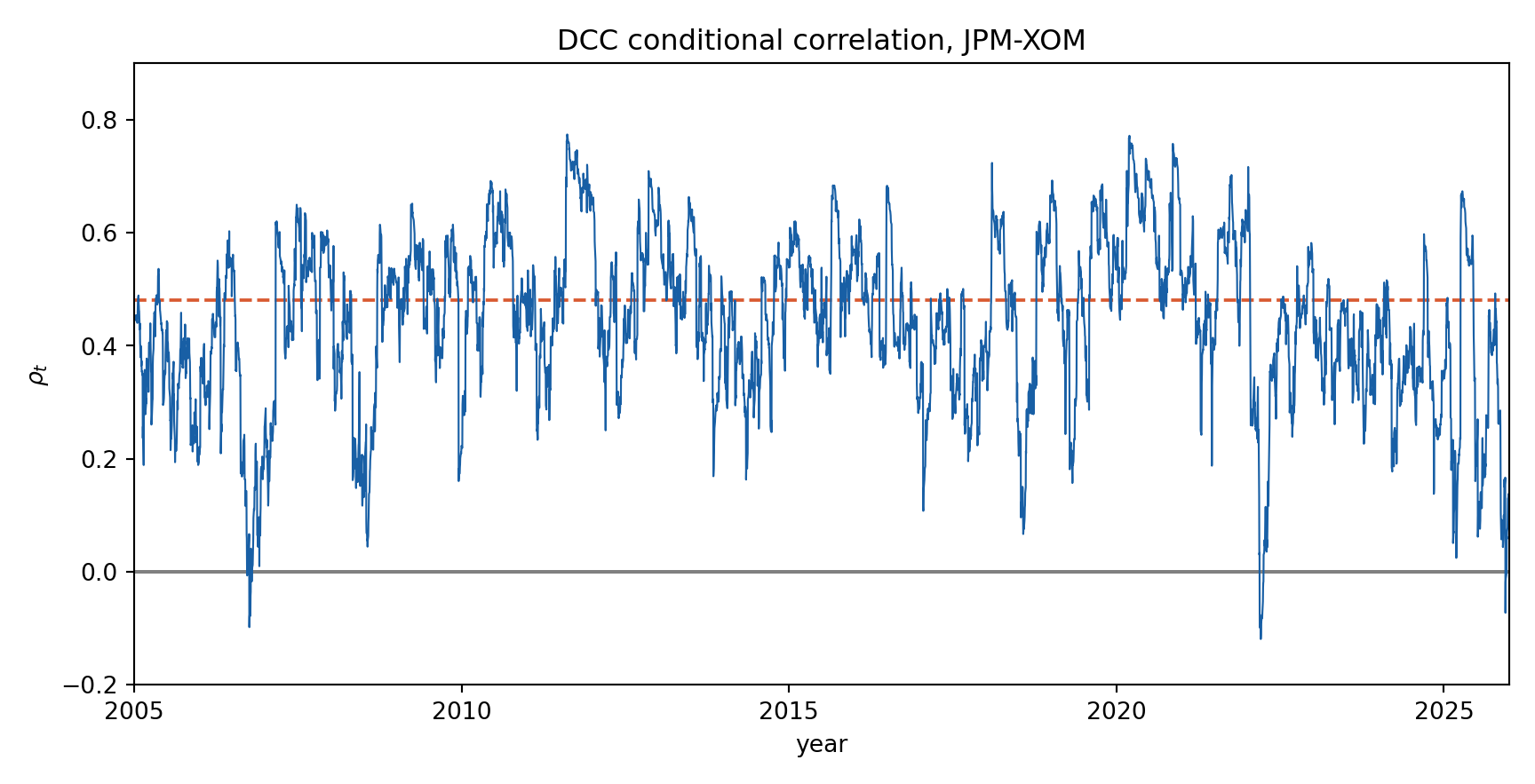
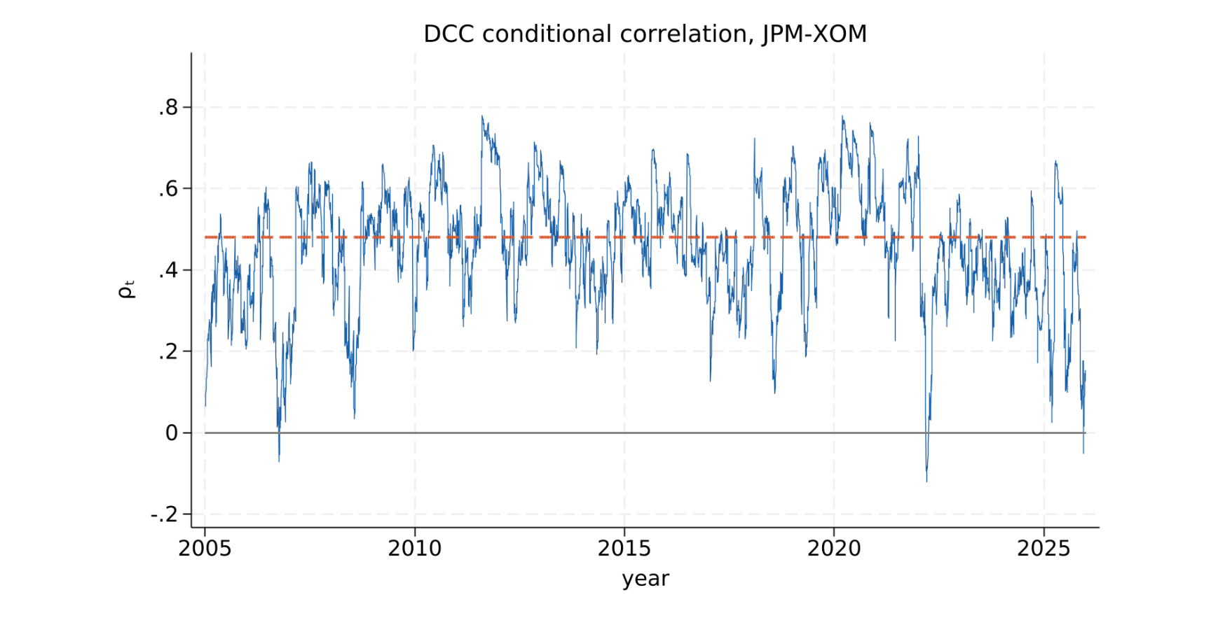
The dashed orange line is the number you would have reported. The blue path is what actually happened.

• The path crosses its own average constantly. It sits near zero through 2006–2007, jumps after the crisis, and is nowhere near \(0.481\) for any sustained period
• The swings are slow, not jumpy. Dependence drifts over months — this is what makes it modellable rather than merely noisy
• The peak is 30 March 2020. At the height of the COVID crash a bank and an oil company moved almost as one asset, \(\rho \approx 0.84\)
• The trough is January 2007. The quietest stretch of the sample, when the two really were close to independent

The last two bullets are the substantive claim of this deck: correlation rises when you least want it to. Diversification is a promise that dependence stays put, and it is withdrawn exactly when it would have paid out.

Note what this plot cannot do. It gives no standard errors, no forecast, and no way to test whether the variation is real rather than sampling noise in a 125-observation window. Parts 2–3 replace it with an estimated model that supplies all three.

The Data

• What & why
• Descriptives
• Reading the descriptives
• Why also simulate

Source. Daily adjusted closing prices from Yahoo Finance, pulled once by dgcop-data.R and written to ../data/dgcop-equity.csv. The window is pinned to 2005-01-04 – 2025-12-30: 5281 trading days, 100×log returns in percent. Deck chunks only ever read that file, so nothing here needs a network connection.

Series	Instrument	Why it is in the sample
spx	S&P 500 index	the “system” — the reference asset for CoVaR and SRISK in Part 6
jpm	JPMorgan Chase	a large bank; the featured series for Stage 1
bac	Bank of America	a second bank, for bank-to-bank contagion
xom	Exxon Mobil	energy; the cross-sector diversification story
gld	SPDR Gold Trust	a safe haven — full-sample correlation with spx is only \(0.056\)
tlt	20+ Year Treasury ETF	duration; correlation with spx is negative, \(-0.313\)

Why these six. Between them they cover every empirical claim the deck makes: two banks for systemic risk, a bank and an oil major for sector diversification, and two assets whose correlation with equities is near zero or negative — which is what makes the hedging and flight-to-quality material in Part 6 possible.

Why US-listed only. All six trade on the same calendar, so the sample is a clean inner join with no missing days to interpolate. Mixing in European or Asian indices would introduce holiday misalignment, and every cross-market correlation would then depend on how those gaps were filled — an arbitrary choice contaminating the quantity being measured.

Why 2005. The window spans three stress episodes of quite different character: the 2008 financial crisis (a slow-building solvency shock), the COVID crash of March 2020 (a sudden exogenous shock), and the 2022 inflation and rate shock (a persistent repricing). A model of time-varying dependence should be judged on more than one kind of crisis.

Why JPM–XOM is the featured pair. Chosen by measurement, not taste. Its full-sample correlation of \(0.481\) looks like comfortable diversification, yet the rolling path runs from \(-0.089\) to \(0.836\) and joint 1% crashes arrive \(2.68\) times more often than a Gaussian copula permits. The single number is wrong in both of the ways this deck is about.

What “reproducible” means here

The CSV is the reproducible artefact, not the download. Yahoo’s adjusted close is revised retroactively whenever a dividend or split occurs, so re-running the download tomorrow can shift historical values by small amounts. Every number on these slides is reproducible from the committed CSV; a fresh download is reproducible only up to those revisions.

Two consequences worth internalising, because they apply to any project built on vendor price data:

• Commit the extract, not just the code. A script that says “download the last 20 years” is not a reproducible specification — the window moves and the history is rewritten beneath it. The window here is pinned to fixed dates for exactly this reason.
• Guard the fetch. dgcop-data.R calls stop() if any series fails or returns fewer than 4000 rows, so a partial download can never quietly become a CSV that then produces plausible-looking but wrong slides.

Adjusted prices are the right choice despite this: unadjusted closes contain artificial jumps on ex-dividend and split dates, which a GARCH model would faithfully interpret as volatility.

eq <- read.csv("../data/dgcop-equity.csv")
series <- c("spx", "jpm", "bac", "xom", "gld", "tlt")

mn <- sdv <- sk <- ku <- mi <- ma <- numeric(length(series))
for (i in seq_along(series)) {
  x  <- eq[[series[i]]]
  m2 <- mean((x - mean(x))^2)
  mn[i]  <- mean(x)
  sdv[i] <- sd(x)
  sk[i]  <- mean((x - mean(x))^3) / m2^1.5
  ku[i]  <- mean((x - mean(x))^4) / m2^2
  mi[i]  <- min(x)
  ma[i]  <- max(x)
}

desc <- data.frame(
  series = series,
  mean   = sprintf("%.3f", mn),
  sd     = sprintf("%.3f", sdv),
  skew   = sprintf("%.3f", sk),
  kurt   = sprintf("%.2f", ku),
  min    = sprintf("%.2f", mi),
  max    = sprintf("%.2f", ma)
)
print(desc, row.names = FALSE)

cat(sprintf("\n%d obs, %s to %s\n", nrow(eq), eq$date[1], eq$date[nrow(eq)]))

 series  mean    sd   skew  kurt    min   max
    spx 0.033 1.209 -0.478 16.21 -12.77 10.96
    jpm 0.051 2.248  0.253 21.15 -23.23 22.39
    bac 0.012 2.869 -0.336 30.25 -34.21 30.21
    xom 0.030 1.666 -0.104 12.61 -15.03 15.86
    gld 0.042 1.114 -0.336  8.87  -9.19 10.70
    tlt 0.013 0.924  0.004  6.41  -6.90  7.25

5281 obs, 2005-01-04 to 2025-12-30

import numpy as np
import pandas as pd
import scipy.stats as st

eq = pd.read_csv("../data/dgcop-equity.csv")
series = ["spx", "jpm", "bac", "xom", "gld", "tlt"]

rows = []
for s in series:
    x = eq[s].values
    rows.append({
        "series": s,
        "mean": f"{x.mean():.3f}",
        "sd":   f"{x.std(ddof=1):.3f}",
        "skew": f"{st.skew(x):.3f}",
        "kurt": f"{st.kurtosis(x, fisher=False):.2f}",
        "min":  f"{x.min():.2f}",
        "max":  f"{x.max():.2f}",
    })

desc = pd.DataFrame(rows)
out = (desc.to_string(index=False) +
       f"\n\n{len(eq)} obs, {eq['date'].iloc[0]} to {eq['date'].iloc[-1]}")
import sys
nw = sys.stdout.write(out + "\n")

series  mean    sd   skew  kurt    min   max
   spx 0.033 1.209 -0.478 16.21 -12.77 10.96
   jpm 0.051 2.248  0.253 21.15 -23.23 22.39
   bac 0.012 2.869 -0.336 30.25 -34.21 30.21
   xom 0.030 1.666 -0.104 12.61 -15.03 15.86
   gld 0.042 1.114 -0.336  8.87  -9.19 10.70
   tlt 0.013 0.924  0.004  6.41  -6.90  7.25

5281 obs, 2005-01-04 to 2025-12-30

sys.stdout.flush()

quietly import delimited "../data/dgcop-equity.csv", clear
tsset t

display "series    mean      sd    skew    kurt      min     max"

* quietly on the loop suppresses Stata's echo of the block structure;
* noisily lets just the display line through
quietly foreach v in spx jpm bac xom gld tlt {
    summarize `v', detail
    noisily display %-6s "`v'" %8.3f r(mean) %8.3f r(sd) %8.3f r(skewness) ///
            %8.2f r(kurtosis) %9.2f r(min) %8.2f r(max)
}

quietly summarize t
local n = r(N)
quietly levelsof date in 1, local(d1) clean
quietly levelsof date in `n', local(d2) clean
display ""
display "`n' obs, `d1' to `d2'"

Time variable: t, 1 to 5281
        Delta: 1 unit

series    mean      sd    skew    kurt      min     max

spx      0.033   1.209  -0.478   16.21   -12.77   10.96
jpm      0.051   2.248   0.253   21.15   -23.23   22.39
bac      0.012   2.869  -0.336   30.25   -34.21   30.21
xom      0.030   1.666  -0.104   12.61   -15.03   15.86
gld      0.042   1.114  -0.336    8.87    -9.19   10.70
tlt      0.013   0.924   0.004    6.41    -6.90    7.25







5281 obs, 2005-01-04 to 2025-12-30

Three features stand out, and each one maps onto a stage of the model.

• Means are economically invisible. Every daily average sits between \(0.01\) and \(0.05\) percent, while standard deviations are 20 to 100 times larger. This is why the deck models the conditional variance and leaves the mean as a constant — at daily frequency there is almost nothing else there
• Every series is heavy-tailed. Kurtosis runs from \(6.41\) (Treasuries) to \(30.25\) (Bank of America), against \(3\) for a normal distribution. No Gaussian assumption survives contact with this table, which is why Student-\(t\) innovations appear from Part 2 onward
• Risk is not uniform. BAC’s standard deviation of \(2.87\) is more than three times TLT’s \(0.92\), and its worst day was \(-34.2\%\). A single portfolio variance cannot be estimated from a single number

The extremes are where the story is. JPM’s worst day, \(-23.2\%\), was 20 January 2009; XOM’s, \(-15.0\%\), was 15 October 2008. Both fall inside the crisis in which the correlation between them was climbing — the joint behaviour that Parts 3 and 4 exist to model.

Real data has one decisive drawback: the true model is unknown. When dccfit reports \(a = 0.035\), nothing in the data says whether that is right.

So the deck carries two simulated companions alongside the real series, built by the same script with the seed 14159 hard-coded:

• dgcop-sim.csv — a bivariate DCC-GARCH system with \(t(8)\) innovations, where \(a\), \(b\) and the whole \(\rho_t\) path are known by construction
• dgcop-copsim.csv — GARCH margins with a time-varying Clayton copula, where \(\lambda_{L,t}\) is known at every date

Every estimator in Parts 2–4 is first pointed at simulated data where the answer is known, and only then at the equity series where it is not. The specifications are on the DGP slides at the end of this part, and the recovery results in Part 3.

Three Stylised Facts

Any model for a pair of financial return series has to reproduce three regularities. They are not exotic; they hold for almost every liquid asset, in every sample, and they are the reason a multivariate normal distribution is the wrong starting point.

1. Volatility clusters

Large moves follow large moves. Returns themselves are barely predictable, but their magnitudes are strongly persistent.

Stage 1 — GARCH

2. Correlation moves

Co-movement tightens in crises and loosens in calm markets, as the previous slide showed.

Stage 2 — DCC

3. Tails depend

Joint crashes happen far more often than a Gaussian model with the right correlation predicts.

Stage 3 — Copula

Fact 1 — and an honest caveat about significance

For JPM over these 5281 days, Ljung–Box with 10 lags gives:

• on returns \(r_t\): \(Q = 103.7\), \(p \approx 10^{-17}\)
• on squared returns \(r_t^2\): \(Q = 3487.5\), \(p \approx 0\)

Both reject. A textbook would like the first not to — and on a shorter sample it would not. The honest reading is about magnitude, not significance:

• the lag-1 autocorrelation of returns is -0.098, and every later lag is under 0.05
• the lag-1 autocorrelation of squared returns is 0.367, and it is still 0.137 at lag 20

The \(Q\) statistic on squares is 34 times larger. With \(T = 5281\) a correlation of \(-0.098\) is comfortably significant and economically almost nothing — it will not survive a bid–ask spread. Statistical significance and economic magnitude part company in large samples, and financial data is where you meet that first.

For contrast, gold (GLD) in the same sample gives \(Q_r = 7.1\), \(p = 0.71\) — the textbook result — while its squared returns still give \(Q = 660\).

Fact 2 — correlation moves

The rolling estimate on the previous slide ranged from -0.089 to 0.836 against a full-sample value of 0.481.

A sceptic should ask whether that is just estimation noise: each window uses only 125 observations, and the standard error of a correlation near \(\rho = 0.48\) at that sample size is roughly

\[ \mathrm{se}(\hat{\rho}) \approx \frac{1 - \rho^2}{\sqrt{w}} \approx \frac{1 - 0.23}{11.2} \approx 0.069 \]

The observed swing is 0.93 wide — about thirteen standard errors. It is not noise.

That informal calculation is exactly what the Engle–Sheppard test formalises in Part 3, where the constant-correlation null is tested properly rather than eyeballed.

Fact 3 — tails depend

Count the days on which JPM and XOM were both below their own 1% quantile, then ask how many a Gaussian copula with \(\rho = 0.481\) would predict:

• observed: 17 joint crashes
• Gaussian copula predicts: 6.3

2.7 times as many as the model allows. At the 5% level it is 89 observed against 61.4 predicted — a ratio of only 1.45. The gap widens as you move further into the tail, which is the signature of tail dependence rather than a plain correlation error.

Note how badly the headline number misleads here. A correlation of \(0.481\) sounds like a well-diversified pair, yet joint disasters arrive nearly three times too often. Raising \(\rho\) cannot repair this, because the Gaussian copula implies

\[ \lambda_L = \lim_{q \to 0} P\bigl(U_1 < q \mid U_2 < q\bigr) = 0 \]

for any \(\rho < 1\). Joint extremes are asymptotically impossible under it. Only changing the copula can fix it — which is the whole argument for Stage 3.

Stylised Facts — Code

Four tests on the JPM return series: two Ljung–Box tests (on \(r_t\) and on \(r_t^2\)), Engle’s ARCH-LM test, and Jarque–Bera for normality.

library(FinTS)     # ArchTest()
library(tseries)   # jarque.bera.test()

d <- eq$jpm

lb_r  <- Box.test(d,   lag = 10, type = "Ljung-Box")
lb_r2 <- Box.test(d^2, lag = 10, type = "Ljung-Box")
arch  <- ArchTest(d, lags = 10)
jb    <- jarque.bera.test(d)

# Box.test returns 1 - pchisq(), which underflows to exactly 0 below ~1e-16.
# Recompute with lower.tail = FALSE so the small p-values stay accurate and
# agree with statsmodels and Stata's chi2tail().
p_lb_r  <- pchisq(lb_r$statistic,  df = 10, lower.tail = FALSE)
p_lb_r2 <- pchisq(lb_r2$statistic, df = 10, lower.tail = FALSE)

# formatted as strings so R, Python and Stata print identical numbers
res <- data.frame(
  test      = c("Ljung-Box r", "Ljung-Box r^2", "ARCH-LM", "Jarque-Bera"),
  statistic = sprintf("%.3f", c(lb_r$statistic, lb_r2$statistic,
                                arch$statistic, jb$statistic)),
  p_value   = sprintf("%.4g", c(p_lb_r, p_lb_r2, arch$p.value, jb$p.value))
)
print(res, row.names = FALSE)

# raw sample moments (n divisor), matching scipy and Stata's summarize, detail
m2 <- mean((d - mean(d))^2)
cat(sprintf("\nskewness = %.3f   kurtosis = %.2f   (normal: 0 and 3)\n",
            mean((d - mean(d))^3) / m2^1.5,
            mean((d - mean(d))^4) / m2^2))

          test statistic    p_value
   Ljung-Box r   103.740  9.698e-18
 Ljung-Box r^2  3487.512          0
       ARCH-LM  1162.756 1.554e-243
   Jarque-Bera 72521.092          0

skewness = 0.253   kurtosis = 21.15   (normal: 0 and 3)

import numpy as np
import pandas as pd
import scipy.stats as st
from statsmodels.stats.diagnostic import acorr_ljungbox, het_arch

d = eq["jpm"].values

lb_r  = acorr_ljungbox(d,    lags=[10])
lb_r2 = acorr_ljungbox(d**2, lags=[10])
arch  = het_arch(d, nlags=10)          # (LM stat, LM p, F stat, F p)
jb    = st.jarque_bera(d)

stats = [lb_r["lb_stat"].iloc[0], lb_r2["lb_stat"].iloc[0], arch[0], jb.statistic]
pvals = [lb_r["lb_pvalue"].iloc[0], lb_r2["lb_pvalue"].iloc[0], arch[1], jb.pvalue]

# formatted as strings so R, Python and Stata print identical numbers
res = pd.DataFrame({
    "test":      ["Ljung-Box r", "Ljung-Box r^2", "ARCH-LM", "Jarque-Bera"],
    "statistic": [f"{v:.3f}" for v in stats],
    "p_value":   [f"{v:.4g}" for v in pvals],
})

out = (res.to_string(index=False) +
       f"\n\nskewness = {st.skew(d):.3f}   "
       f"kurtosis = {st.kurtosis(d, fisher=False):.2f}   (normal: 0 and 3)")
import sys
nw = sys.stdout.write(out + "\n")

         test statistic    p_value
  Ljung-Box r   103.740  9.698e-18
Ljung-Box r^2  3487.512          0
      ARCH-LM  1162.756 1.554e-243
  Jarque-Bera 72521.092          0

skewness = 0.253   kurtosis = 21.15   (normal: 0 and 3)

sys.stdout.flush()

quietly import delimited "../data/dgcop-equity.csv", clear
tsset t
quietly gen double jpm2 = jpm^2

* Ljung-Box portmanteau on returns and on squared returns
quietly wntestq jpm, lags(10)
display "Ljung-Box r    : Q = " %9.3f r(stat) "   p = " %9.4g r(p)
quietly wntestq jpm2, lags(10)
display "Ljung-Box r^2  : Q = " %9.3f r(stat) "   p = " %9.4g r(p)

* Engle's ARCH-LM: regress squared returns on 10 of their own lags, LM = n * R^2.
* Written out rather than taken from estat archlm so that all three languages
* compute the identical statistic.
quietly regress jpm2 L(1/10).jpm2
scalar lm = e(N) * e(r2)
display "ARCH-LM        : LM = " %9.3f lm "   p = " %9.4g chi2tail(10, lm)

* Jarque-Bera, computed from the sample moments
quietly summarize jpm, detail
scalar sk = r(skewness)
scalar ku = r(kurtosis)
scalar jb = _N * (sk^2/6 + (ku - 3)^2/24)
display "Jarque-Bera    : JB = " %9.3f jb "   p = " %9.4g chi2tail(2, jb)
display ""
display "skewness = " %6.3f sk "   kurtosis = " %5.2f ku "   (normal: 0 and 3)"

Time variable: t, 1 to 5281
        Delta: 1 unit



Ljung-Box r    : Q =   103.740   p =  9.70e-18


Ljung-Box r^2  : Q =  3487.512   p =         0



ARCH-LM        : LM =  1162.756   p =  1.6e-243





Jarque-Bera    : JB = 72521.094   p =         0



skewness =  0.253   kurtosis = 21.15   (normal: 0 and 3)

Stylised Facts — Plot

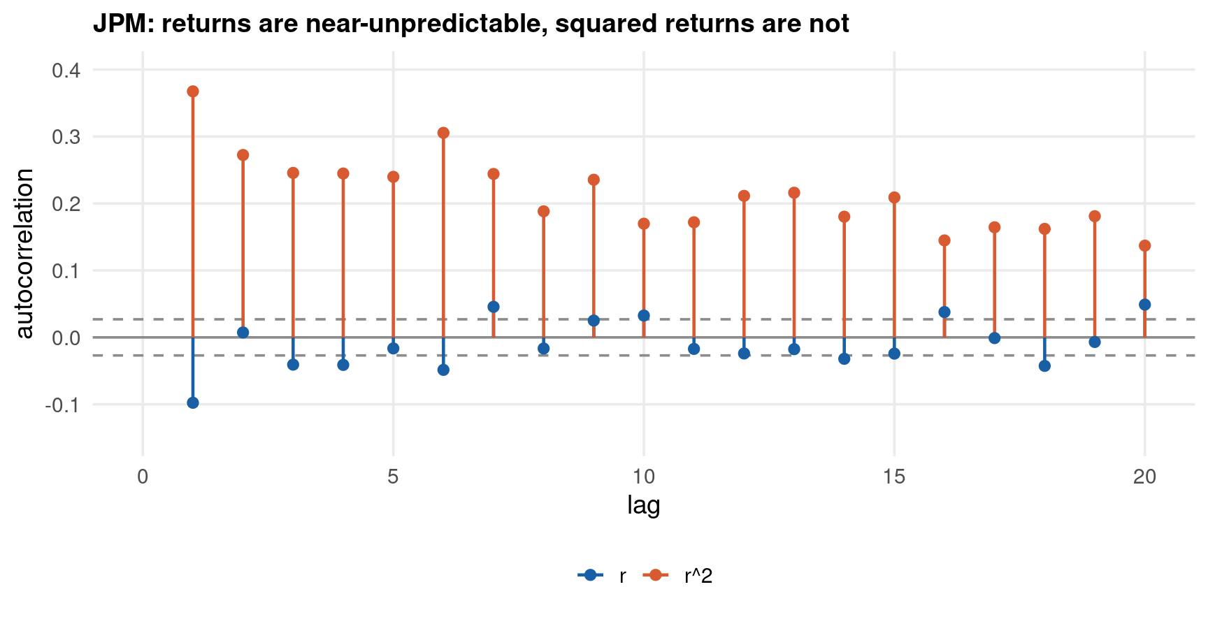
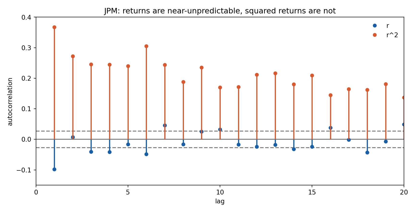
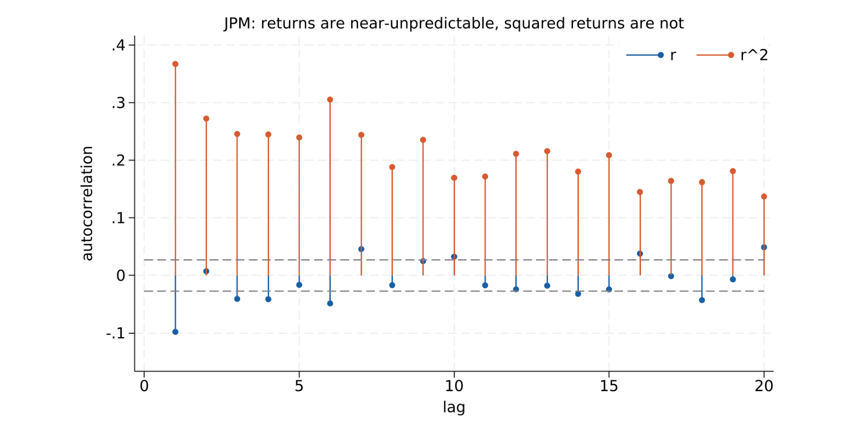
The autocorrelation function of \(r_t\) against that of \(r_t^2\), on one pair of axes. Both are computed from the same formula so the three languages agree exactly:

\[ \hat{\gamma}_k \;=\; \frac{\sum_{t=k+1}^{T} (x_t - \bar{x})(x_{t-k} - \bar{x})} {\sum_{t=1}^{T} (x_t - \bar{x})^2} \qquad \text{band} = \pm \frac{1.96}{\sqrt{T}} \]

acf_hand <- function(x, K = 20) {
  xc  <- x - mean(x)
  den <- sum(xc^2)
  out <- numeric(K)
  for (k in 1:K) {
    out[k] <- sum(xc[(k + 1):length(xc)] * xc[1:(length(xc) - k)]) / den
  }
  out
}

d    <- eq$jpm
band <- 1.96 / sqrt(length(d))

adf <- data.frame(lag = rep(1:20, 2),
                  acf = c(acf_hand(d), acf_hand(d^2)),
                  series = rep(c("r", "r^2"), each = 20))

ggplot(adf) +
  aes(x = lag, y = acf, colour = series) +
  geom_hline(yintercept = 0, colour = "grey55") +
  geom_hline(yintercept = c(-band, band), colour = "grey55", linetype = "dashed") +
  geom_segment(aes(xend = lag, yend = 0), linewidth = 0.8) +
  geom_point(size = 2.2) +
  scale_colour_manual(values = c("r" = "#185FA5", "r^2" = "#D85A30")) +
  coord_cartesian(xlim = c(0, 20), ylim = c(-0.15, 0.40)) +
  scale_x_continuous(breaks = seq(0, 20, 5)) +
  scale_y_continuous(breaks = seq(-0.1, 0.4, 0.1)) +
  labs(x = "lag", y = "autocorrelation", colour = NULL,
       title = "JPM: returns are near-unpredictable, squared returns are not")

import matplotlib.pyplot as plt

def acf_hand(x, K=20):
    xc  = x - x.mean()
    den = (xc**2).sum()
    return np.array([(xc[k:] * xc[:-k]).sum() / den for k in range(1, K + 1)])

d    = eq["jpm"].values
band = 1.96 / np.sqrt(len(d))
lags = np.arange(1, 21)

fig, ax = plt.subplots(figsize=(9, 4.6))
ax.axhline(0, color="grey")
ax.axhline(band,  color="grey", linestyle="--")
ax.axhline(-band, color="grey", linestyle="--")
for vals, col, lab in [(acf_hand(d), "#185FA5", "r"),
                       (acf_hand(d**2), "#D85A30", "r^2")]:
    ax.vlines(lags, 0, vals, color=col, linewidth=1.8)
    ax.plot(lags, vals, "o", color=col, markersize=5, label=lab)
ax.legend(frameon=False)
axopts = ax.set(xlim=(0, 20), ylim=(-0.15, 0.40),
                xticks=range(0, 21, 5),
                yticks=np.arange(-0.10, 0.41, 0.10),
                xlabel="lag", ylabel="autocorrelation",
                title="JPM: returns are near-unpredictable, squared returns are not")
plt.tight_layout()
plt.show()

quietly import delimited "../data/dgcop-equity.csv", clear
tsset t
quietly gen double jpm2 = jpm^2

* Hand-coded ACF, identical formula to the R and Python tabs
quietly summarize jpm
quietly gen double c1 = jpm - r(mean)
quietly summarize jpm2
quietly gen double c2 = jpm2 - r(mean)
quietly gen double s1 = c1^2
quietly gen double s2 = c2^2
quietly summarize s1
scalar den1 = r(sum)
quietly summarize s2
scalar den2 = r(sum)

quietly gen int    klag = _n if _n <= 20
quietly gen double a1   = .
quietly gen double a2   = .
quietly forvalues k = 1/20 {
    gen double p1 = c1 * L`k'.c1
    gen double p2 = c2 * L`k'.c2
    summarize p1
    replace a1 = r(sum)/den1 in `k'
    summarize p2
    replace a2 = r(sum)/den2 in `k'
    drop p1 p2
}
scalar band = 1.96 / sqrt(5281)

twoway (dropline a1 klag, lcolor("24 95 165") mcolor("24 95 165") msize(small))   ///
       (dropline a2 klag, lcolor("216 90 48") mcolor("216 90 48") msize(small))   ///
       (function y = band,  range(0 20) lcolor(gs8) lpattern(dash))               ///
       (function y = -band, range(0 20) lcolor(gs8) lpattern(dash)),              ///
    legend(order(1 "r" 2 "r^2") rows(1) position(1) ring(0) region(lstyle(none))) ///
    xscale(range(0 20)) xlabel(0(5)20)                                            ///
    yscale(range(-0.15 0.40)) ylabel(-0.10(0.10)0.40)                             ///
    xtitle("lag") ytitle("autocorrelation")                                       ///
    title("JPM: returns are near-unpredictable, squared returns are not", size(medsmall)) ///
    graphregion(color(white)) plotregion(color(white))

graph export "../plots/dgcop-p1-acf.png", replace width(1600)

The Cost of Ignoring Them

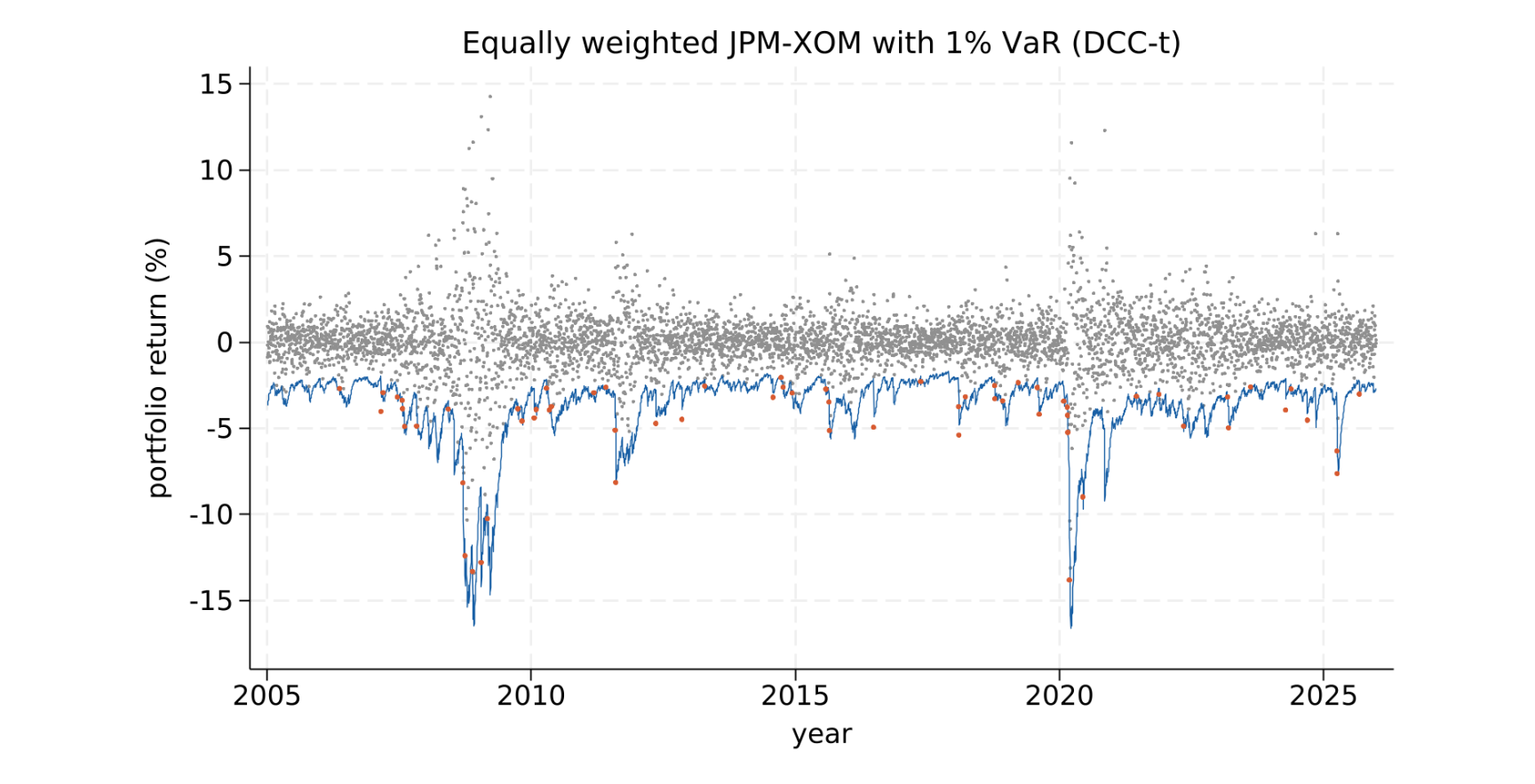
A concrete price tag, before any theory. Hold an equally weighted JPM/XOM portfolio and compute a 1% one-day Value-at-Risk three ways, then count how often the realised loss was worse than the forecast. Over 5281 days, a correct 1% VaR should be breached about 53 times.

• Result
• Reading it
• How it was computed

                                   model facts_used violations rate_pct
           Gaussian, constant vol & corr       none         89     1.69
     CCC-GARCH  (vol varies, corr fixed)          1         89     1.69
 DCC-t      (vol & corr vary, fat tails)  1 + 2 + 3         67     1.27

expected violations at 1% over 5281 days: 53

CCC constant correlation = 0.4468    DCC rho_t range = -0.117 to 0.773

DCC-t estimated degrees of freedom = 6.13

The ranking is the entire argument for the next six parts, and it is monotone:

• Ignore everything — 89 breaches where 53 were expected, a 68% overshoot, and they arrive in clusters during exactly the weeks that matter
• Model volatility only (fact 1) — 89 breaches. Exactly the same count, and that is the interesting part
• Model volatility, correlation and tails (facts 1–3) — 67 breaches against 53 expected

The first two rows are identical, which is not what students expect. Modelling volatility alone buys nothing in violation count here: the CCC model still fixes the correlation at \(0.4468\) for twenty-one years, while the true path runs from \(-0.117\) to \(0.773\). Getting the variances right while the correlation is wrong leaves the portfolio variance wrong anyway. The gain arrives only when the correlation is allowed to move and the innovations are allowed fat tails — the estimated \(\nu \approx 6.1\) is far from Gaussian.

Note also that these are in-sample counts, which flatter every model — each one saw the data it is being judged on. Part 5 redoes this honestly, out of sample, with Kupiec, Christoffersen and DQ tests attached, and the ordering survives.

port <- 0.5 * eq$jpm + 0.5 * eq$xom          # equally weighted

# A — unconditional Gaussian: one mean, one variance, for all 5281 days
var_a <- mean(port) + qnorm(0.01) * sd(port)

# B — CCC: GARCH(1,1) per series, correlation fixed at the sample value
#     of the standardised residuals
var_b <- mu_b + qnorm(0.01) *
         sqrt(0.25*s1^2 + 0.25*s2^2 + 2*0.25*rho_ccc*s1*s2)

# C — DCC-t: correlation follows the DCC recursion, innovations Student-t
sd_p  <- sqrt(0.25*Hc[,1]^2 + 0.25*Hc[,2]^2 +
              2*0.25*Rc[1,2,]*Hc[,1]*Hc[,2])
var_c <- mu_c + qt(0.01, df = nu) * sqrt((nu - 2)/nu) * sd_p

# a violation is a day whose realised return fell below the forecast
sum(port < var_c)

The portfolio standard deviation uses the textbook identity

\[ \sigma_{p,t}^2 \;=\; w_1^2 h_{1,t} + w_2^2 h_{2,t} + 2 w_1 w_2 \rho_t \sqrt{h_{1,t} h_{2,t}} \]

with \(w_1 = w_2 = 1/2\). Only the treatment of \(h_{i,t}\) and \(\rho_t\) changes between the three rows — which is what makes the comparison fair.

Literature — Foundations

The framework is an assembly of four separate literatures, each solving one piece.

Year	Contribution	Authors	DOI
1959	Copulas: separating margins from dependence	Sklar	hal-04094463
1982	ARCH — conditional variance as a model object	Engle	10.2307/1912773
1986	GARCH — parsimonious volatility persistence	Bollerslev	10.1016/0304-4076(86)90063-1
1990	CCC — constant conditional correlation	Bollerslev	10.2307/2109358
1991	EGARCH — asymmetric volatility response	Nelson	10.2307/2938260
1993	GJR — leverage via a threshold term	Glosten, Jagannathan, Runkle	10.1111/j.1540-6261.1993.tb05128.x
1996	IFM — two-stage estimation for copula models	Joe, Xu	UBC TR 166
2001	Test for constant correlation	Engle, Sheppard	10.3386/w8554
2002	DCC — correlation with its own recursion	Engle	10.1198/073500102288618487
2002	VCC — an alternative dynamic correlation	Tse, Tsui	10.1198/073500102288618496
2006	Time-varying copula	Patton	10.1111/j.1468-2354.2006.00387.x

Read in order, these are four answers to the same question — what is conditional on what? Engle (1982) made the variance conditional; Bollerslev (1990) left the correlation unconditional; Engle (2002) made it conditional too; Patton (2006) made the entire dependence structure conditional.

Literature — Four Modern Strands

• Fixing DCC
• Dynamic copulas
• High dimensions
• Risk & systemic risk

Engle’s estimator works, but its properties took a decade to pin down and some remain unresolved.

• Aielli (2013) — the standard DCC estimator of \(\bar{Q}\) is inconsistent; cDCC repairs it. 10.1080/07350015.2013.771027
• Cappiello, Engle, Sheppard (2006) — ADCC adds asymmetry, so correlation responds more to joint bad news. 10.1093/jjfinec/nbl005
• Caporin, McAleer (2013) — a sceptical reading: DCC has no known large-\(N\) asymptotics and is best seen as a filter, not an estimator. 10.3390/econometrics1010115
• Bauwens, Laurent, Rombouts (2006) — the survey that maps the whole MGARCH family. 10.1002/jae.842

• Patton (2006) — the founding paper: let the copula parameter follow an ARMA-type recursion. 10.1111/j.1468-2354.2006.00387.x
• Creal, Koopman, Lucas (2013) — GAS: drive the parameter by the score of its own likelihood, which gives one recipe for every family. 10.1002/jae.1279
• Manner, Reznikova (2012) — a survey of the competing time-varying designs. 10.1080/07474938.2011.608042
• Patton (2013) — the Handbook chapter, the best single entry point. 10.1016/B978-0-444-62731-5.00016-6

• Engle, Ledoit, Wolf (2019) — nonlinear shrinkage makes DCC usable for hundreds of assets. 10.1080/07350015.2017.1345683
• Colacito, Engle, Ghysels (2011) — DCC-MIDAS splits correlation into a slow and a fast component. 10.1016/j.jeconom.2011.02.013
• Oh, Patton (2017) — factor copulas: dependence through a small number of common shocks. 10.1080/07350015.2015.1062384
• Brechmann, Czado (2013) — vine copulas on GARCH-filtered residuals. 10.1524/strm.2013.2002

• Christoffersen (1998) — interval forecasts: violations must be both correctly counted and independent. 10.2307/2527341
• Engle, Manganelli (2004) — the DQ test, which detects clustered breaches. 10.1198/073500104000000370
• Adrian, Brunnermeier (2016) — CoVaR: system risk conditional on one institution failing. 10.1257/aer.20120555
• Brownlees, Engle (2017) — SRISK: expected capital shortfall in a crisis. 10.1093/rfs/hhw060
• Fissler, Ziegel (2016) — ES is not elicitable alone, but is jointly with VaR. 10.1214/16-AOS1439

What the Applied Literature Found

• The studies
• What generalises
• What this deck adds

The papers above build the machinery. These use it, and their results are the closest thing to a prior you can bring to Part 4’s family choice.

Year	Data & model	What they found	Authors	DOI
2002	US equity portfolios, exceedance correlation	Correlation with the market is higher in downturns than upturns — the asymmetry that motivated everything after it	Ang, Chen	10.1016/S0304-405X(02)00068-5
2006	DEM/USD and JPY/USD, time-varying copula	Dependence is asymmetric and it moves — the founding empirical application	Patton	10.1111/j.1468-2354.2006.00387.x
2007	East Asian & Latin American crises, switching copula	The dependence structure changes regime in a crisis, not merely its parameter	Rodriguez	10.1016/j.jempfin.2006.07.002
2011	BRIC–US equity, time-varying copula	Strong extreme interdependence; contagion strongest where economic structure links the markets	Aloui, Ben Aïssa, Nguyen	10.1016/j.jbankfin.2010.07.021
2011	crude oil benchmarks, several families	Symmetric upper and lower tail dependence — oil is “one great pool”	Reboredo	10.1016/j.eneco.2011.04.006
2012	developed & emerging equity, dynamic asymmetric copula	Correlations and tail dependence both rose; diversification benefits shrank, least so in emerging markets	Christoffersen, Errunza, Jacobs, Langlois	10.1093/rfs/hhs104
2013	international equity, long-memory margins + copula	Copula-based portfolios beat mean–variance once dependence is modelled properly	Boubaker, Sghaier	10.1016/j.jbankfin.2012.09.006
2016	equity, FX, commodities; EVT margins + pair-copulas	Stress-test losses are badly understated by benchmark risk models	Koliai	10.1016/j.jbankfin.2016.02.004
2018	energy vs agricultural commodities, switching CoVaR-copula	Spillover is direction-dependent — Part 6’s CoVaR applied to commodities	Ji, Bouri, Roubaud, Shahzad	10.1016/j.eneco.2018.08.015

Three claims survive across these papers, and one popular claim does not.

• Equity dependence is asymmetric. Ang–Chen, Patton and Christoffersen et al. all find joint crashes are more likely than joint booms. A Gaussian copula, which forces \(\lambda_L = \lambda_U = 0\), is rejected on equity data routinely.
• Dependence is not stable. Rodriguez finds the structure switches, not merely the parameter — which is why Part 7 tests for breaks rather than assuming one regime.
• The tails drive the risk numbers. Koliai’s stress-test losses and Christoffersen’s diversification result both come from tail behaviour the marginals cannot produce alone.

The claim that does not generalise: “Student-\(t\) fits equities, Clayton fits commodities.” It is repeated often enough to sound like a stylised fact, and Reboredo (2011) contradicts it directly — crude oil benchmarks show symmetric tail dependence, the opposite of Clayton’s lower-tail skew. Asymmetry is a property of the pair, not of the asset class. Ji et al. find switching dependence in energy–agriculture, Reboredo finds symmetry within oil. Test for it; do not assume it from the ticker.

Every study above reports a fitted model. Almost none reports what the model costs when it is wrong, and that is where this deck differs.

• Part 4 fits five copulas to one pair and compares them on likelihood, not on convention
• Part 5 turns each into a VaR series and backtests it, where every model fails the independence test
• Part 7 asks whether the extra machinery — dynamic copulas, vines, shrinkage, ML — actually beat the simple alternative, and on this data it did not

The honest summary of the applied literature is that model choice matters most in the tails, and least where the papers spend most of their space.

Copulas in 60 Seconds

The companion deck Copula Methods in Economics and Econometrics develops this material in full. Here is the minimum needed to follow Stage 3.

Sklar’s theorem (1959). Any joint distribution can be split into its margins and a dependence function:

\[ F(x_1, x_2) \;=\; C\bigl(F_1(x_1),\, F_2(x_2)\bigr) \]

with \(C\) unique whenever the margins are continuous. Margins and dependence can therefore be modelled — and estimated — separately.

The probability integral transform. Feed each variable through its own CDF:

\[ u_i \;=\; F_i(x_i) \;\sim\; \mathrm{Uniform}(0,1) \]

The pair \((u_1, u_2)\) carries all the dependence and none of the marginal shape.

Tail dependence. The quantity this deck cares about most:

\[ \lambda_L \;=\; \lim_{q \to 0^+} P\bigl(U_1 \le q \mid U_2 \le q\bigr), \qquad \lambda_U \;=\; \lim_{q \to 1^-} P\bigl(U_1 > q \mid U_2 > q\bigr) \]

Gaussian copula: \(\lambda_L = \lambda_U = 0\) for any \(\rho < 1\). Student-\(t\): \(\lambda_L = \lambda_U > 0\). Clayton: \(\lambda_L > 0\), \(\lambda_U = 0\).

Where the two decks divide. The copula deck asks what shape is the dependence? — families, estimation, goodness-of-fit, vines. This deck asks how does that shape change from day to day, and what does the change cost in risk capital? Everything from here on is conditional dependence.

Notation & the Three-Stage Roadmap

• The three stages
• Notation

The model is built in three passes over the same data, each removing one feature and handing the remainder to the next.

Stage	Object	Removes	Output
1	Univariate GARCH per series	volatility clustering	\(\hat{h}_{i,t}\), standardised residuals \(\hat{z}_{i,t}\)
2	DCC on \(\hat{z}_t\)	time-varying linear correlation	\(\hat{R}_t\), the path \(\hat{\rho}_{ij,t}\)
3	Copula on PIT residuals \(\hat{u}_t\)	remaining non-linear / tail dependence	\(\hat{\theta}\), \(\hat{\lambda}_L\), \(\hat{\lambda}_U\)

This is the IFM (inference functions for margins) strategy of Joe and Xu (1996): estimate the pieces in sequence rather than jointly. It is consistent and computationally cheap. It is not fully efficient, and Part 3 shows exactly what that costs — the three languages disagree on the DCC parameters for precisely this reason.

Returns, decomposed into a conditional mean and a shock:

\[ r_{i,t} \;=\; \mu_i + \varepsilon_{i,t}, \qquad \varepsilon_{i,t} \;=\; \sqrt{h_{i,t}}\; z_{i,t} \]

with \(z_{i,t}\) standardised, \(E[z_{i,t}] = 0\) and \(\mathrm{Var}(z_{i,t}) = 1\). The conditional covariance matrix factors as

\[ H_t \;=\; D_t R_t D_t, \qquad D_t = \mathrm{diag}\bigl(\sqrt{h_{1,t}},\, \sqrt{h_{2,t}}\bigr) \]

so that \(D_t\) holds everything univariate and \(R_t\) everything about dependence. The copula acts on the transformed residuals

\[ u_{i,t} \;=\; F_i\bigl(\hat{z}_{i,t}\bigr) \]

Symbol	Meaning
\(h_{i,t}\)	conditional variance of series \(i\) at time \(t\)
\(z_{i,t}\)	standardised innovation
\(D_t\)	diagonal matrix of conditional standard deviations
\(R_t\)	conditional correlation matrix
\(Q_t\)	the auxiliary DCC matrix (not itself a correlation matrix)
\(\bar{Q}\)	unconditional correlation of the \(\hat{z}_t\) — the DCC target
\(u_{i,t}\)	PIT residual, uniform on \([0,1]\) under correct specification
\(\lambda_L, \lambda_U\)	lower / upper tail dependence

DGP — Mathematical Specification

Two simulated systems accompany the real data. Both are written by dgcop-data.R; the deck only reads them. Simulation is what lets us check that an estimator recovers a known answer before we trust it on data where no answer exists.

• DCC-GARCH system
• Time-varying copula system

Two series, GARCH(1,1) margins, multivariate-\(t\) innovations, \(T = 2000\):

\[ h_{1,t} = 0.05 + 0.08\,\varepsilon_{1,t-1}^2 + 0.90\,h_{1,t-1}, \qquad h_{2,t} = 0.03 + 0.06\,\varepsilon_{2,t-1}^2 + 0.92\,h_{2,t-1} \]

The correlation follows the DCC recursion with targeting:

\[ Q_t \;=\; (1 - a - b)\,\bar{Q} \;+\; a\, z_{t-1} z_{t-1}' \;+\; b\, Q_{t-1}, \qquad a = 0.03,\; b = 0.95 \]

\[ R_t \;=\; \mathrm{diag}(Q_t)^{-1/2}\, Q_t \,\mathrm{diag}(Q_t)^{-1/2}, \qquad \bar{Q} = \begin{pmatrix} 1 & 0.5 \\ 0.5 & 1 \end{pmatrix} \]

with \(z_t \sim t_\nu(0, R_t)\) standardised to unit variance, \(\nu = 8\).

GARCH(1,1) margins again, but dependence now comes from a Clayton copula whose parameter moves, following Patton (2006). With \(\Lambda(x) = (1 + e^{-x})^{-1}\) and \(T = 1500\):

\[ f_t \;=\; 1.0 \;+\; 0.80\, f_{t-1} \;-\; 5.0 \cdot \frac{1}{10}\sum_{j=1}^{10} \bigl|u_{t-j} - v_{t-j}\bigr| \]

\[ \theta_t \;=\; 0.50 \;+\; 1.15 \cdot \Lambda(f_t) \]

The forcing term is the mean absolute distance between the two PIT series over the last ten periods: when the pair moves together it is small, which pushes \(\theta_t\) up. Lower tail dependence follows directly:

\[ \lambda_{L,t} \;=\; 2^{-1/\theta_t} \]

The bounds on \(\theta_t\) hold \(\lambda_{L,t}\) inside \([0.25,\, 0.66]\) by construction, so the design does not depend on the draw.

DGP — Code Implementation

The DCC-GARCH system, as written in dgcop-data.R. The seed 14159 is hard-coded so any of these blocks reproduces the series standalone.

set.seed(14159)
n_sim <- 2000; burn <- 500; N <- n_sim + burn
om1 <- 0.05; al1 <- 0.08; be1 <- 0.90
om2 <- 0.03; al2 <- 0.06; be2 <- 0.92
dcc_a <- 0.03; dcc_b <- 0.95; rho_bar <- 0.50; nu <- 8

Qbar <- matrix(c(1, rho_bar, rho_bar, 1), 2, 2)
h1 <- numeric(N); h2 <- numeric(N)
e1 <- numeric(N); e2 <- numeric(N); rho <- numeric(N)
h1[1] <- om1/(1 - al1 - be1); h2[1] <- om2/(1 - al2 - be2)
Q <- Qbar; zvec <- c(0, 0)

for (i in seq_len(N)) {
  if (i > 1) {
    h1[i] <- om1 + al1 * e1[i-1]^2 + be1 * h1[i-1]
    h2[i] <- om2 + al2 * e2[i-1]^2 + be2 * h2[i-1]
    Q <- (1 - dcc_a - dcc_b) * Qbar + dcc_a * (zvec %*% t(zvec)) + dcc_b * Q
  }
  rho[i] <- Q[1,2] / sqrt(Q[1,1] * Q[2,2])

  # standardised multivariate t: N(0, R_t) scaled by sqrt((nu-2)/w), w ~ chi2(nu)
  R <- matrix(c(1, rho[i], rho[i], 1), 2, 2)
  g <- as.numeric(t(chol(R)) %*% rnorm(2))
  zvec <- g * sqrt((nu - 2) / rchisq(1, df = nu))
  e1[i] <- sqrt(h1[i]) * zvec[1]
  e2[i] <- sqrt(h2[i]) * zvec[2]
}

import numpy as np

rng = np.random.default_rng(14159)
n_sim, burn = 2000, 500
N = n_sim + burn
om1, al1, be1 = 0.05, 0.08, 0.90
om2, al2, be2 = 0.03, 0.06, 0.92
dcc_a, dcc_b, rho_bar, nu = 0.03, 0.95, 0.50, 8

Qbar = np.array([[1.0, rho_bar], [rho_bar, 1.0]])
h1 = np.zeros(N); h2 = np.zeros(N)
e1 = np.zeros(N); e2 = np.zeros(N); rho = np.zeros(N)
h1[0] = om1/(1 - al1 - be1); h2[0] = om2/(1 - al2 - be2)
Q = Qbar.copy(); z = np.zeros(2)

for i in range(N):
    if i > 0:
        h1[i] = om1 + al1*e1[i-1]**2 + be1*h1[i-1]
        h2[i] = om2 + al2*e2[i-1]**2 + be2*h2[i-1]
        Q = (1 - dcc_a - dcc_b)*Qbar + dcc_a*np.outer(z, z) + dcc_b*Q
    rho[i] = Q[0, 1] / np.sqrt(Q[0, 0]*Q[1, 1])

    R = np.array([[1.0, rho[i]], [rho[i], 1.0]])
    g = np.linalg.cholesky(R) @ rng.standard_normal(2)
    z = g * np.sqrt((nu - 2) / rng.chisquare(nu))
    e1[i] = np.sqrt(h1[i]) * z[0]
    e2[i] = np.sqrt(h2[i]) * z[1]

clear
set seed 14159
set obs 2500                      // 2000 kept + 500 burn-in
gen int t = _n
tsset t

scalar om1 = 0.05
scalar al1 = 0.08
scalar be1 = 0.90
scalar om2 = 0.03
scalar al2 = 0.06
scalar be2 = 0.92
scalar a   = 0.03
scalar b   = 0.95
scalar rb  = 0.50
scalar nu  = 8

gen double h1 = om1/(1 - al1 - be1)
gen double h2 = om2/(1 - al2 - be2)
gen double e1 = 0
gen double e2 = 0
gen double rho = rb
gen double q11 = 1
gen double q22 = 1
gen double q12 = rb
gen double z1 = 0
gen double z2 = 0

quietly forvalues i = 2/2500 {
    replace h1 = om1 + al1*e1[`i'-1]^2 + be1*h1[`i'-1] in `i'
    replace h2 = om2 + al2*e2[`i'-1]^2 + be2*h2[`i'-1] in `i'
    replace q11 = (1-a-b) + a*z1[`i'-1]^2 + b*q11[`i'-1] in `i'
    replace q22 = (1-a-b) + a*z2[`i'-1]^2 + b*q22[`i'-1] in `i'
    replace q12 = (1-a-b)*rb + a*z1[`i'-1]*z2[`i'-1] + b*q12[`i'-1] in `i'
    replace rho = q12[`i']/sqrt(q11[`i']*q22[`i']) in `i'

    * standardised bivariate t via Cholesky of R_t and a chi2 mixing variable
    local w = rchi2(nu)
    replace z1 = rnormal()*sqrt((nu-2)/`w') in `i'
    replace z2 = (rho[`i']*z1[`i'] + sqrt(1-rho[`i']^2)*rnormal()*sqrt((nu-2)/`w')) in `i'
    replace e1 = sqrt(h1[`i'])*z1[`i'] in `i'
    replace e2 = sqrt(h2[`i'])*z2[`i'] in `i'
}
drop in 1/500

DGP — Diagnostics

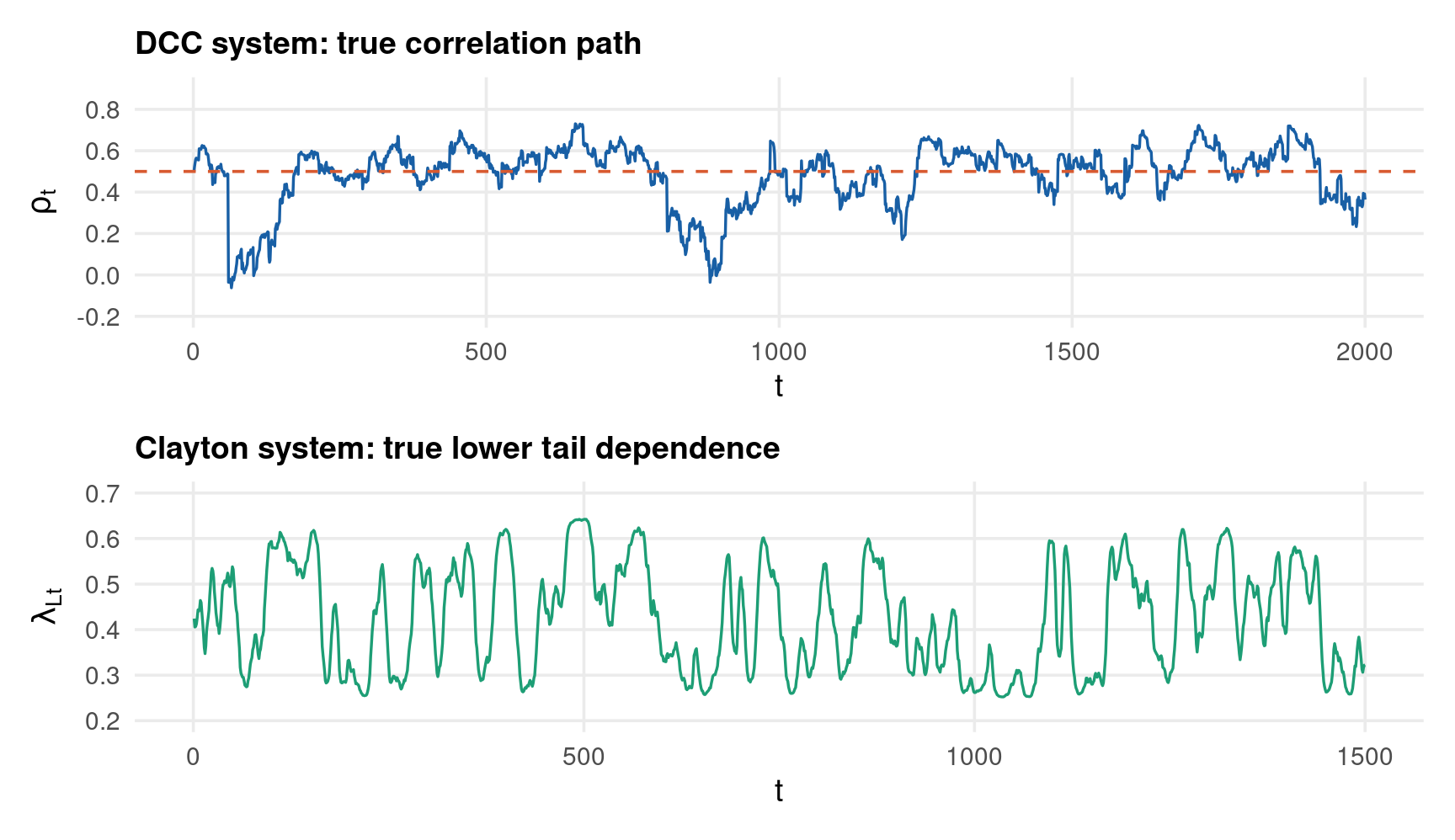
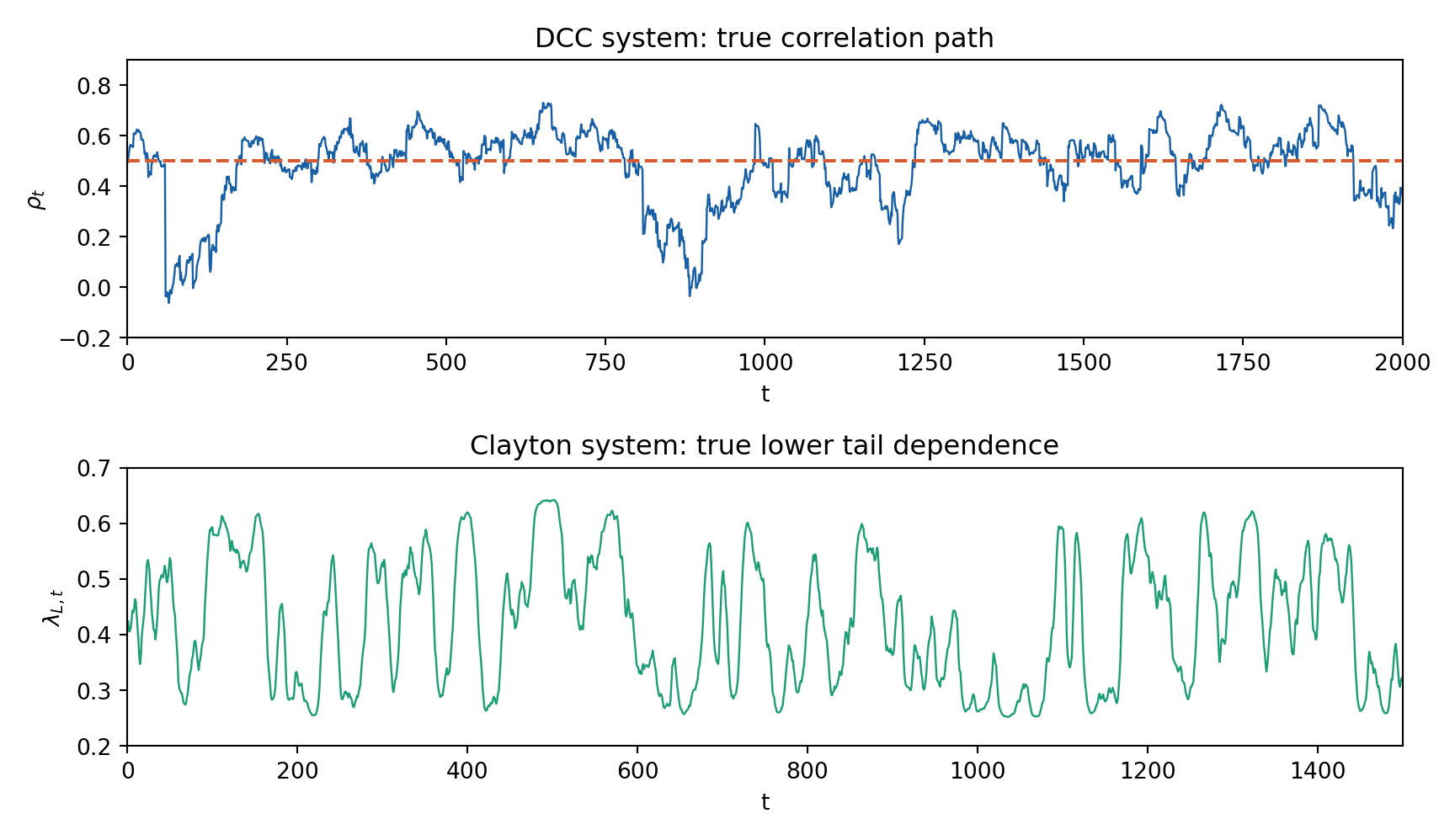
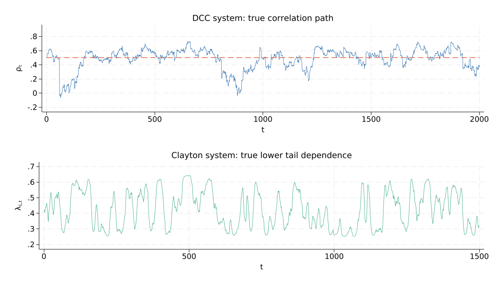
Does the simulated data actually contain what it was designed to contain? Two checks, one per system: the DCC correlation path, and the Clayton tail-dependence path. Both are stored in the CSVs as rho_true and lambda_l_true.

library(patchwork)

sim <- read.csv("../data/dgcop-sim.csv")
cop <- read.csv("../data/dgcop-copsim.csv")

p1 <- ggplot(sim) +
  aes(x = t, y = rho_true) +
  geom_line(colour = "#185FA5", linewidth = 0.6) +
  geom_hline(yintercept = 0.50, colour = "#D85A30", linetype = "dashed") +
  coord_cartesian(xlim = c(0, 2000), ylim = c(-0.2, 0.9)) +
  labs(x = "t", y = expression(rho[t]), title = "DCC system: true correlation path")

p2 <- ggplot(cop) +
  aes(x = t, y = lambda_l_true) +
  geom_line(colour = "#1D9E75", linewidth = 0.6) +
  coord_cartesian(xlim = c(0, 1500), ylim = c(0.20, 0.70)) +
  labs(x = "t", y = expression(lambda[L * t]),
       title = "Clayton system: true lower tail dependence")

p1 / p2

import matplotlib.pyplot as plt
import pandas as pd

sim = pd.read_csv("../data/dgcop-sim.csv")
cop = pd.read_csv("../data/dgcop-copsim.csv")

fig, (ax1, ax2) = plt.subplots(2, 1, figsize=(9, 5.2))

ax1.plot(sim["t"], sim["rho_true"], color="#185FA5", linewidth=0.9)
ax1.axhline(0.50, color="#D85A30", linestyle="--")
o1 = ax1.set(xlim=(0, 2000), ylim=(-0.2, 0.9),
             yticks=[-0.2, 0.0, 0.2, 0.4, 0.6, 0.8],
             xlabel="t", ylabel=r"$\rho_t$",
             title="DCC system: true correlation path")

ax2.plot(cop["t"], cop["lambda_l_true"], color="#1D9E75", linewidth=0.9)
o2 = ax2.set(xlim=(0, 1500), ylim=(0.20, 0.70),
             yticks=[0.2, 0.3, 0.4, 0.5, 0.6, 0.7],
             xlabel="t", ylabel=r"$\lambda_{L,t}$",
             title="Clayton system: true lower tail dependence")

plt.tight_layout()
plt.show()

quietly import delimited "../data/dgcop-sim.csv", clear
tsset t
twoway (line rho_true t, lcolor("24 95 165") lwidth(vthin))              ///
       (function y = 0.5, range(0 2000) lcolor("216 90 48") lpattern(dash)), ///
    legend(off) xscale(range(0 2000)) xlabel(0(500)2000)                 ///
    yscale(range(-0.2 0.9)) ylabel(-0.2(0.2)0.8)                         ///
    xtitle("t") ytitle("{&rho}{sub:t}")                                  ///
    title("DCC system: true correlation path", size(medium))             ///
    graphregion(color(white)) plotregion(color(white)) name(g1, replace)

quietly import delimited "../data/dgcop-copsim.csv", clear
tsset t
twoway (line lambda_l_true t, lcolor("29 158 117") lwidth(vthin)),       ///
    legend(off) xscale(range(0 1500)) xlabel(0(500)1500)                 ///
    yscale(range(0.20 0.70)) ylabel(0.2(0.1)0.7)                         ///
    xtitle("t") ytitle("{&lambda}{sub:L,t}")                             ///
    title("Clayton system: true lower tail dependence", size(medium))    ///
    graphregion(color(white)) plotregion(color(white)) name(g2, replace)

graph combine g1 g2, rows(2) graphregion(color(white)) xsize(9) ysize(5.2)
graph export "../plots/dgcop-p1-dgpdiag.png", replace width(1600)

Part 2 — Stage 1: GARCH Margins

κακὸν κακῷ διάδοχον ἐν τῇδ’ ἡμέρᾳ πορσύνεται.

one trouble succeeds another, and within a single day

Εὐριπίδης, Ἀνδρομάχη 802–803

The GARCH Family — Theory & Math

• Idea
• Math

Stage 1 treats each series on its own. Nothing about dependence enters yet — the job is to strip out volatility clustering so that what remains is close to i.i.d., and can be handed to Stage 2 as clean input.

The single idea behind every model here: the variance of tomorrow’s return is known today, as a function of what has already happened.

• A large shock today raises tomorrow’s variance — that is the ARCH term \(\alpha\)
• Yesterday’s variance persists into today — that is the GARCH term \(\beta\)
• Together they generate clustering without any change in the mean equation

Four variants are worth knowing, and they differ in exactly one respect: how a shock of size \(\varepsilon_{t-1}\) enters.

• sGARCH — only the square of the shock matters, so \(+5\%\) and \(-5\%\) are identical
• GJR — negative shocks get an extra loading \(\gamma\)
• EGARCH — models \(\log h_t\), so positivity is automatic and asymmetry is built in
• APARCH — the power itself is estimated rather than fixed at 2

Innovations are Student-\(t\) throughout, not Gaussian. Part 1 measured JPM’s kurtosis at \(21.15\); a GARCH model with normal innovations cannot reproduce that even with volatility clustering, because the clustering alone generates only mild excess kurtosis.

Returns split into a constant mean and a shock scaled by conditional volatility:

\[ r_t \;=\; \mu + \varepsilon_t, \qquad \varepsilon_t \;=\; \sqrt{h_t}\, z_t, \qquad z_t \sim t_\nu \; \text{standardised to unit variance} \]

sGARCH(1,1) — Bollerslev (1986):

\[ h_t \;=\; \omega + \alpha \varepsilon_{t-1}^2 + \beta h_{t-1}, \qquad \omega > 0,\; \alpha, \beta \ge 0 \]

GJR(1,1) — Glosten, Jagannathan and Runkle (1993), with \(I_{t-1} = \mathbf{1}\{\varepsilon_{t-1} < 0\}\):

\[ h_t \;=\; \omega + \bigl(\alpha + \gamma I_{t-1}\bigr)\varepsilon_{t-1}^2 + \beta h_{t-1} \]

EGARCH(1,1) — Nelson (1991), in logs so no positivity constraint is needed:

\[ \log h_t \;=\; \omega + \alpha z_{t-1} + \gamma\bigl(|z_{t-1}| - E|z_{t-1}|\bigr) + \beta \log h_{t-1} \]

Covariance stationarity requires, for sGARCH,

\[ \alpha + \beta < 1 \]

and the unconditional variance and shock half-life then follow:

\[ \bar{h} \;=\; \frac{\omega}{1 - \alpha - \beta}, \qquad \text{half-life} \;=\; \frac{\log 0.5}{\log(\alpha + \beta)} \]

The GARCH Family — Code

sGARCH(1,1) with Student-\(t\) innovations, fitted to JPM.

library(rugarch)

eq <- read.csv("../data/dgcop-equity.csv")

spec <- ugarchspec(
  variance.model = list(model = "sGARCH", garchOrder = c(1, 1)),
  mean.model     = list(armaOrder = c(0, 0), include.mean = TRUE),
  distribution.model = "std"          # standardised Student-t
)
fit <- ugarchfit(spec, eq$jpm)

print(round(fit@fit$matcoef, 6))
cat(sprintf("\nlog-likelihood = %.3f   n = %d\n", likelihood(fit), nrow(eq)))

        Estimate  Std. Error   t value Pr(>|t|)
mu      0.090460    0.016827  5.375885    0e+00
omega   0.046280    0.010378  4.459294    8e-06
alpha1  0.099780    0.012359  8.073185    0e+00
beta1   0.891528    0.012657 70.434985    0e+00
shape   5.042483    0.348402 14.473157    0e+00

log-likelihood = -9760.634   n = 5281

import numpy as np
import pandas as pd
from arch import arch_model

eq = pd.read_csv("../data/dgcop-equity.csv")
d  = eq["jpm"].values

# backcast fixes the pre-sample variance h_0 at the sample variance, which is
# what rugarch and Stata use. Without it arch() applies an EWMA backcast and the
# estimates differ in the third decimal - see the popup on the next slide.
bc  = float(np.var(d))
res = arch_model(d, mean="Constant", vol="GARCH", p=1, q=1,
                 dist="t").fit(disp="off", backcast=bc)

tab = pd.DataFrame({
    "Estimate":  [f"{v:.6f}" for v in res.params],
    "Std.Error": [f"{v:.6f}" for v in res.std_err],
    "t value":   [f"{v:.4f}" for v in res.tvalues],
    "Pr(>|t|)":  [f"{v:.4g}" for v in res.pvalues],
}, index=res.params.index)

out = (tab.to_string() +
       f"\n\nlog-likelihood = {res.loglikelihood:.3f}   n = {len(d)}")
import sys
nw = sys.stdout.write(out + "\n")

          Estimate Std.Error  t value   Pr(>|t|)
mu        0.090478  0.016638   5.4379   5.39e-08
omega     0.046324  0.012467   3.7157  0.0002026
alpha[1]  0.099671  0.016059   6.2066  5.415e-10
beta[1]   0.891540  0.017082  52.1930          0
nu        5.046262  0.349739  14.4287  3.417e-47

log-likelihood = -9760.635   n = 5281

sys.stdout.flush()

quietly import delimited "../data/dgcop-equity.csv", clear
tsset t

arch jpm, arch(1) garch(1) distribution(t)

Time variable: t, 1 to 5281
        Delta: 1 unit


(setting optimization to BHHH)
Iteration 0:  Log likelihood = -10295.996  
Iteration 1:  Log likelihood = -9954.5942  
Iteration 2:  Log likelihood = -9837.8286  
Iteration 3:  Log likelihood =  -9773.555  
Iteration 4:  Log likelihood = -9762.3245  
(switching optimization to BFGS)
Iteration 5:  Log likelihood = -9760.8178  
Iteration 6:  Log likelihood = -9760.6403  
Iteration 7:  Log likelihood = -9760.6366  
Iteration 8:  Log likelihood = -9760.6362  
Iteration 9:  Log likelihood = -9760.6362  
Iteration 10: Log likelihood = -9760.6362  

ARCH family regression

Sample: 1 thru 5281                             Number of obs     =       5281
                                                Wald chi2(.)      =          .
Log likelihood = -9760.636                      Prob > chi2       =          .

------------------------------------------------------------------------------
             |                 OPG
         jpm | Coefficient  std. err.      z    P>|z|     [95% conf. interval]
-------------+----------------------------------------------------------------
jpm          |
       _cons |     .09046    .017065     5.30   0.000     .0570132    .1239068
-------------+----------------------------------------------------------------
ARCH         |
        arch |
         L1. |   .0996773   .0097676    10.20   0.000     .0805331    .1188214
             |
       garch |
         L1. |    .891533   .0093725    95.12   0.000     .8731632    .9099028
             |
       _cons |   .0463277   .0090861     5.10   0.000     .0285193     .064136
-------------+----------------------------------------------------------------
     /lndfm2 |   1.113892   .1141697     9.76   0.000      .890123     1.33766
-------------+----------------------------------------------------------------
          df |    5.04619   .3477827                      4.435429    5.810118
------------------------------------------------------------------------------

The GARCH Family — Results & Interpretation

• How to run
• Reading the output

Mean equation. A constant is enough at daily frequency. Part 1 found a lag-1 autocorrelation of \(-0.098\) in JPM returns — statistically significant, but too small to be worth an ARMA term, and the GARCH filter removes most of it anyway (the Ljung–Box statistic on standardised residuals falls from \(103.7\) to \(13.5\)).

Order. \((1,1)\) almost always. Higher orders rarely improve fit and often produce a \(\beta\) against its boundary. Test rather than assume — the model selection slide does exactly that.

Distribution. std in rugarch, dist="t" in arch, distribution(t) in Stata. All three estimate \(\nu\) rather than fixing it.

The one argument that matters for reproducibility. Python’s arch initialises the recursion with an EWMA backcast; rugarch and Stata use the sample variance. Pass backcast=np.var(d) and all three agree.

Why the three languages disagreed, and how to fix it

The GARCH recursion needs a value for \(h_0\) before the first observation. It is not estimated, it is chosen, and the packages choose differently:

• rugarch and Stata use the sample variance of the series
• arch (Python) uses an exponentially weighted backcast of the squared residuals

With \(T = 5281\) that choice should be irrelevant, and asymptotically it is. It is not irrelevant in the third decimal:

• default backcast: \(\omega = 0.043408\), \(\alpha = 0.094531\), \(\beta = 0.896695\), \(\ell = -9757.01\)
• backcast=np.var(d): \(\omega = 0.046324\), \(\alpha = 0.099671\), \(\beta = 0.891540\), \(\ell = -9760.635\)
• rugarch: \(\omega = 0.046280\), \(\alpha = 0.099780\), \(\beta = 0.891528\), \(\ell = -9760.634\)

Note the log-likelihoods are not comparable across the first two lines — they condition on different pre-sample assumptions, so the “better” likelihood of the default is not evidence of a better fit.

The general lesson. When two packages disagree on a model they both claim to implement, the difference is almost never in the optimiser. Look first at what happens before the sample starts: initial conditions, burn-in, and degrees-of-freedom conventions. Part 3 shows the same phenomenon at the multivariate level, where the choice is between two-stage and joint estimation.

                        quantity   value
       persistence  alpha + beta  0.9913
     half-life of a shock (days) 79.3992
      unconditional sd (daily %)  2.3075
 unconditional sd (annualised %) 36.6301
             sample sd (daily %)  2.2485
                  tail index  nu  5.0425

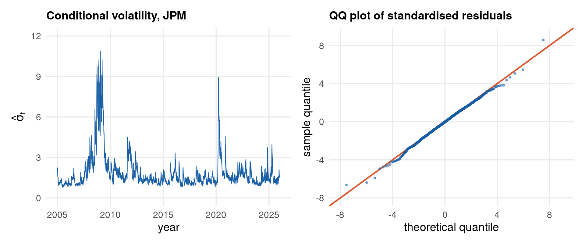
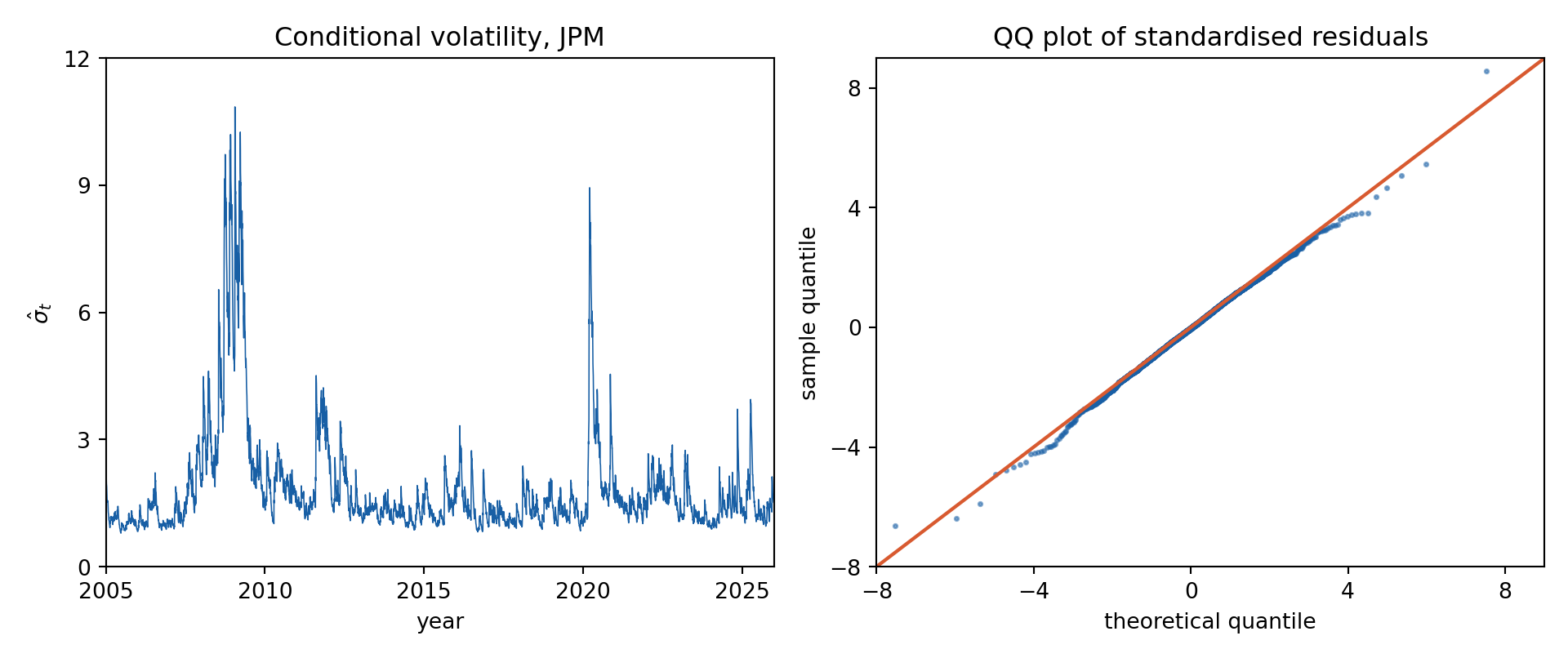
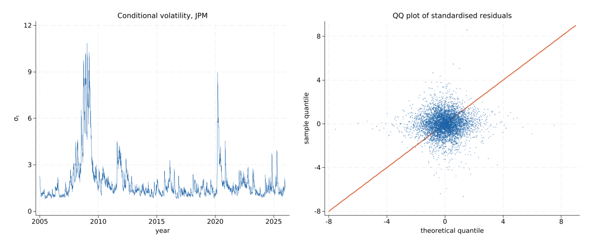
peak conditional volatility 10.86 on 2009-01-22

• \(\alpha + \beta = 0.9913\). Volatility is extremely persistent but still stationary. A shock takes about 79 trading days — four months — to decay by half
• \(\nu \approx 5.0\). Even after removing volatility clustering the innovations are far from normal. A \(t_5\) has infinite kurtosis beyond the fourth moment; this is the single strongest argument against Gaussian risk models
• Unconditional volatility \(2.31\%\) daily, about \(36.6\%\) annualised, close to the raw sample standard deviation of \(2.25\%\) — a sanity check that the model has not drifted somewhere implausible
• \(\beta \gg \alpha\). Variance is far more a function of its own past than of yesterday’s surprise. This is why volatility forecasts are so much easier than return forecasts

How close to the boundary is 0.9913?

Close enough to matter. The half-life is \(\log(0.5)/\log(\alpha+\beta)\), and that function explodes as the sum approaches one:

• \(\alpha + \beta = 0.95 \Rightarrow\) half-life 14 days
• \(\alpha + \beta = 0.99 \Rightarrow\) half-life 69 days
• \(\alpha + \beta = 0.9913 \Rightarrow\) half-life 79 days
• \(\alpha + \beta = 0.999 \Rightarrow\) half-life 693 days

A difference of \(0.04\) in the estimate changes the economic conclusion by a factor of five. Report the persistence with its standard error, never as a bare point estimate.

At exactly 1 the model becomes IGARCH: the unconditional variance \(\omega/(1-\alpha-\beta)\) is undefined and shocks never die. Empirically, estimates this close to unity are often a symptom of an unmodelled structural break in the variance rather than genuine long memory — a quiet regime shift makes the variance look permanently displaced. Part 7 returns to this under regime switching.

Note also what persistence is not: it says nothing about predictability of returns. \(\beta = 0.89\) describes variance, and a highly forecastable variance is entirely consistent with an unforecastable mean.

Leverage — Theory & Math

• Idea
• Math

sGARCH squares the shock, so a \(-5\%\) day and a \(+5\%\) day leave identical variance forecasts. Markets do not behave that way: bad news raises volatility more than good news of the same size.

The standard names for the mechanism:

• Leverage effect (Black 1976) — a price fall raises the debt-to-equity ratio, so the equity becomes mechanically riskier
• Volatility feedback — anticipated higher volatility raises required returns, pushing prices down now, so causality runs the other way
• Behavioural — trading intensity and disagreement rise more after losses

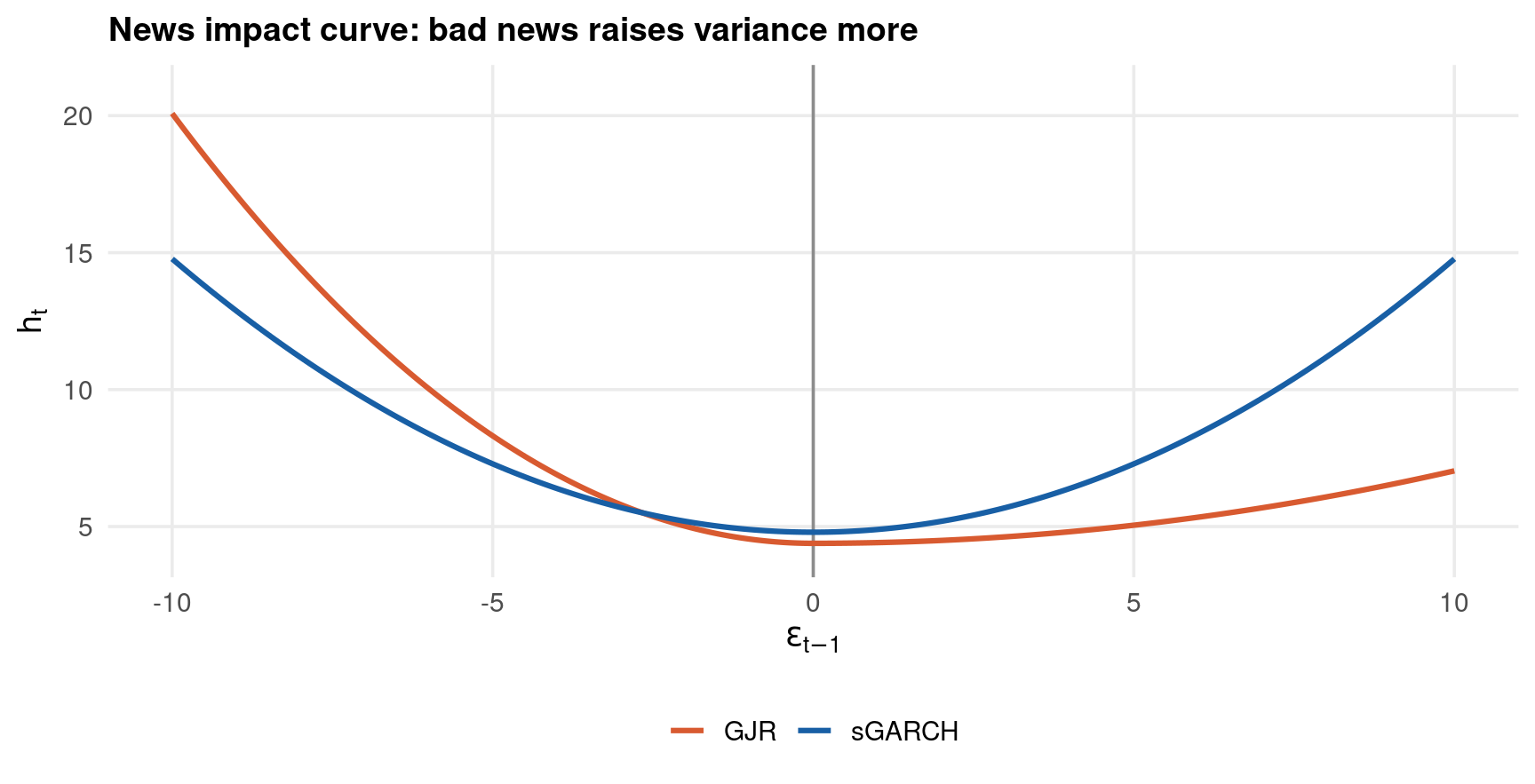
Which mechanism dominates is unsettled; that the asymmetry exists is not. The news impact curve makes it visible: plot next period’s variance as a function of this period’s shock, holding everything else at its unconditional level.

The news impact curve fixes \(h_{t-1}\) at \(\bar{h}\) and varies \(\varepsilon_{t-1}\):

\[ \text{NIC}(\varepsilon) \;=\; h_t \bigm| \bigl(\varepsilon_{t-1} = \varepsilon,\; h_{t-1} = \bar{h}\bigr) \]

For sGARCH it is a symmetric parabola, minimised at zero:

\[ \text{NIC}_{\text{sGARCH}}(\varepsilon) \;=\; \omega + \beta \bar{h} + \alpha \varepsilon^2 \]

For GJR the left branch is steeper:

\[ \text{NIC}_{\text{GJR}}(\varepsilon) \;=\; \omega + \beta \bar{h} + \begin{cases} (\alpha + \gamma)\,\varepsilon^2 & \varepsilon < 0 \\[2pt] \alpha\,\varepsilon^2 & \varepsilon \ge 0 \end{cases} \]

so the asymmetry is one number, \(\gamma > 0\). The GJR unconditional variance picks up the extra term at its expected frequency:

\[ \bar{h}_{\text{GJR}} \;=\; \frac{\omega}{1 - \alpha - \beta - \gamma/2} \]

using \(P(\varepsilon_{t-1} < 0) = 1/2\) for a symmetric innovation distribution.

Leverage — Code

spec_gjr <- ugarchspec(
  variance.model = list(model = "gjrGARCH", garchOrder = c(1, 1)),
  mean.model     = list(armaOrder = c(0, 0), include.mean = TRUE),
  distribution.model = "std"
)
fit_gjr <- ugarchfit(spec_gjr, eq$jpm)
cg <- coef(fit_gjr)

cat(sprintf("alpha (good news load) = %.5f\n", cg["alpha1"]))
cat(sprintf("gamma (extra for bad)  = %.5f\n", cg["gamma1"]))
cat(sprintf("alpha + gamma (bad)    = %.5f\n", cg["alpha1"] + cg["gamma1"]))
cat(sprintf("ratio bad / good       = %.2f\n",
            (cg["alpha1"] + cg["gamma1"]) / cg["alpha1"]))

alpha (good news load) = 0.02646

gamma (extra for bad)  = 0.13047

alpha + gamma (bad)    = 0.15693

ratio bad / good       = 5.93

# o=1 adds the asymmetric (threshold) term to the GARCH recursion
res_gjr = arch_model(d, mean="Constant", vol="GARCH", p=1, o=1, q=1,
                     dist="t").fit(disp="off", backcast=bc)
pg = res_gjr.params

out = (f"alpha (good news load) = {pg['alpha[1]']:.5f}\n"
       f"gamma (extra for bad)  = {pg['gamma[1]']:.5f}\n"
       f"alpha + gamma (bad)    = {pg['alpha[1]'] + pg['gamma[1]']:.5f}\n"
       f"ratio bad / good       = "
       f"{(pg['alpha[1]'] + pg['gamma[1]']) / pg['alpha[1]']:.2f}")
import sys
nw = sys.stdout.write(out + "\n")

alpha (good news load) = 0.02642
gamma (extra for bad)  = 0.13031
alpha + gamma (bad)    = 0.15674
ratio bad / good       = 5.93

sys.stdout.flush()

quietly import delimited "../data/dgcop-equity.csv", clear
tsset t

* Stata's tarch() is the same GJR model in a mirrored parameterisation:
* its indicator switches on POSITIVE shocks, so _b[ARCH:L1.arch] is the
* BAD-news load and the tarch coefficient is negative.
quietly arch jpm, arch(1) garch(1) tarch(1) distribution(t)

scalar bad  = _b[ARCH:L1.arch]
scalar good = _b[ARCH:L1.arch] + _b[ARCH:L1.tarch]

display "alpha (good news load) = " %8.5f good
display "gamma (extra for bad)  = " %8.5f -_b[ARCH:L1.tarch]
display "alpha + gamma (bad)    = " %8.5f bad
display "ratio bad / good       = " %8.2f bad/good

Time variable: t, 1 to 5281
        Delta: 1 unit




alpha (good news load) =  0.02618

gamma (extra for bad)  =  0.13062

alpha + gamma (bad)    =  0.15680

ratio bad / good       =     5.99

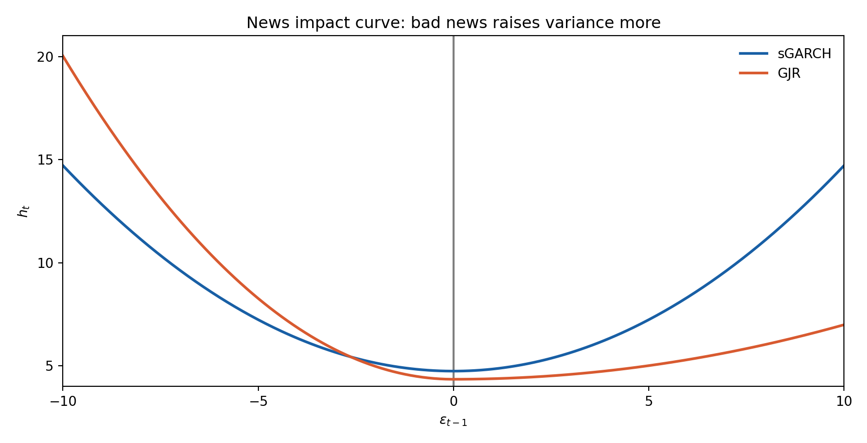
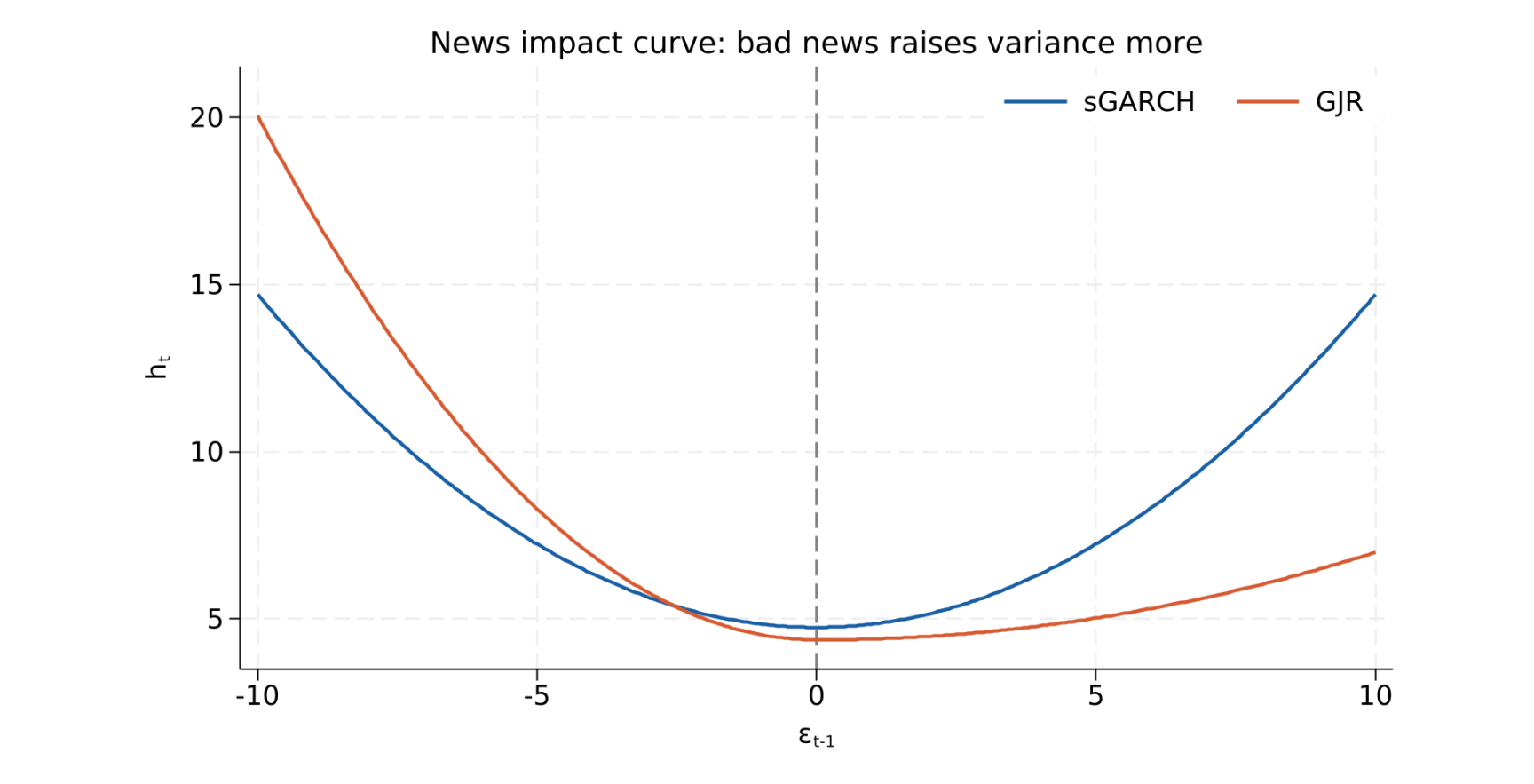
Leverage — News Impact Curve

Both curves are drawn from the fitted coefficients on a common grid \(\varepsilon \in [-10, 10]\), with \(h_{t-1}\) held at each model’s own \(\bar{h}\).

cs  <- coef(fit)
s2s <- cs["omega"] / (1 - cs["alpha1"] - cs["beta1"])
s2g <- cg["omega"] / (1 - cg["alpha1"] - cg["beta1"] - 0.5 * cg["gamma1"])

e   <- seq(-10, 10, length.out = 401)
nic <- data.frame(
  eps   = rep(e, 2),
  h     = c(cs["omega"] + cs["alpha1"] * e^2 + cs["beta1"] * s2s,
            cg["omega"] + (cg["alpha1"] + cg["gamma1"] * (e < 0)) * e^2 +
              cg["beta1"] * s2g),
  model = rep(c("sGARCH", "GJR"), each = length(e))
)

ggplot(nic) +
  aes(x = eps, y = h, colour = model) +
  geom_vline(xintercept = 0, colour = "grey55") +
  geom_line(linewidth = 1.1) +
  scale_colour_manual(values = c("sGARCH" = "#185FA5", "GJR" = "#D85A30")) +
  coord_cartesian(xlim = c(-10, 10), ylim = c(4, 21)) +
  scale_x_continuous(breaks = seq(-10, 10, 5)) +
  scale_y_continuous(breaks = seq(5, 20, 5)) +
  labs(x = expression(epsilon[t-1]), y = expression(h[t]), colour = NULL,
       title = "News impact curve: bad news raises variance more")

import matplotlib.pyplot as plt

ps  = res.params
s2s = ps["omega"] / (1 - ps["alpha[1]"] - ps["beta[1]"])
s2g = pg["omega"] / (1 - pg["alpha[1]"] - pg["beta[1]"] - 0.5 * pg["gamma[1]"])

e    = np.linspace(-10, 10, 401)
h_s  = ps["omega"] + ps["alpha[1]"] * e**2 + ps["beta[1]"] * s2s
h_g  = (pg["omega"] + (pg["alpha[1]"] + pg["gamma[1]"] * (e < 0)) * e**2
        + pg["beta[1]"] * s2g)

fig, ax = plt.subplots(figsize=(9, 4.6))
ax.axvline(0, color="grey")
ax.plot(e, h_s, color="#185FA5", linewidth=2.0, label="sGARCH")
ax.plot(e, h_g, color="#D85A30", linewidth=2.0, label="GJR")
ax.legend(frameon=False)
axopts = ax.set(xlim=(-10, 10), ylim=(4, 21),
                xticks=range(-10, 11, 5), yticks=[5, 10, 15, 20],
                xlabel=r"$\varepsilon_{t-1}$", ylabel=r"$h_t$",
                title="News impact curve: bad news raises variance more")
plt.tight_layout()
plt.show()

quietly import delimited "../data/dgcop-equity.csv", clear
tsset t

quietly arch jpm, arch(1) garch(1) distribution(t)
scalar om_s = _b[ARCH:_cons]
scalar al_s = _b[ARCH:L1.arch]
scalar be_s = _b[ARCH:L1.garch]
scalar s2s  = om_s/(1 - al_s - be_s)

quietly arch jpm, arch(1) garch(1) tarch(1) distribution(t)
scalar om_g = _b[ARCH:_cons]
scalar bad  = _b[ARCH:L1.arch]
scalar good = _b[ARCH:L1.arch] + _b[ARCH:L1.tarch]
scalar be_g = _b[ARCH:L1.garch]
scalar s2g  = om_g/(1 - good - be_g - 0.5*(bad - good))

twoway (function y = om_s + al_s*x^2 + be_s*s2s, range(-10 10)                 ///
            lcolor("24 95 165") lwidth(medthick))                              ///
       (function y = om_g + cond(x<0, bad, good)*x^2 + be_g*s2g,               ///
            range(-10 10) lcolor("216 90 48") lwidth(medthick)),               ///
    xline(0, lcolor(gs8))                                                      ///
    legend(order(1 "sGARCH" 2 "GJR") rows(1) position(1) ring(0)               ///
           region(lstyle(none)))                                               ///
    xscale(range(-10 10)) xlabel(-10(5)10)                                     ///
    yscale(range(4 21)) ylabel(5(5)20)                                         ///
    xtitle("{&epsilon}{sub:t-1}") ytitle("h{sub:t}")                           ///
    title("News impact curve: bad news raises variance more", size(medium))    ///
    graphregion(color(white)) plotregion(color(white))

graph export "../plots/dgcop-p2-nic.png", replace width(1600)

The GJR curve is the point of the slide. A shock of \(-4\) implies \(h_t = 6.90\); the same shock with a \(+\) sign implies \(4.81\) — a 43% higher variance forecast after identical-sized bad news. In loading terms the asymmetry is much starker: bad news enters at \(0.157\), good news at \(0.026\), a factor of 5.9.

Model Selection — Theory & Math

• Idea
• Math

Four candidate models, all fitted to the same data by maximum likelihood, all nested or non-nested in awkward combinations. Likelihood alone cannot choose: adding parameters can never lower it.

Information criteria penalise dimension. Both of the standard ones take the form “minus twice the log-likelihood plus a penalty per parameter”, and they differ only in how hard they penalise.

• AIC — penalty \(2k\); targets predictive accuracy, tends to over-fit slightly in large samples
• BIC — penalty \(k \log T\); targets the true model, and with \(T = 5281\) it penalises about \(4.3\) times harder than AIC

When they disagree, say so and report both. Here they do not disagree, which makes the conclusion easy.

For a model with \(k\) parameters and maximised log-likelihood \(\hat{\ell}\):

\[ \mathrm{AIC} \;=\; -2\hat{\ell} + 2k, \qquad \mathrm{BIC} \;=\; -2\hat{\ell} + k \log T \]

Lower is better for both. A caution specific to this comparison:

\[ \log T \;=\; \log 5281 \;=\; 8.572 \;\gg\; 2 \]

so BIC is far more conservative about extra parameters than AIC.

Report totals, not averages. rugarch divides its information criteria by \(T\), while arch and Stata report totals. The ranking is unaffected, but the numbers are not comparable across packages unless one convention is imposed — so all three tabs below compute \(-2\hat{\ell} + 2k\) by hand.

Model Selection — Code & Results

models <- c("sGARCH", "gjrGARCH", "eGARCH", "apARCH")
nm <- llh <- k <- numeric(0)

for (m in models) {
  sp <- ugarchspec(variance.model = list(model = m, garchOrder = c(1, 1)),
                   mean.model = list(armaOrder = c(0, 0), include.mean = TRUE),
                   distribution.model = "std")
  f  <- ugarchfit(sp, eq$jpm, solver = "hybrid")
  llh <- c(llh, likelihood(f))
  k   <- c(k, length(coef(f)))
}

n   <- nrow(eq)
sel <- data.frame(
  model = models, k = k,
  logLik = sprintf("%.3f", llh),
  AIC    = sprintf("%.2f", -2 * llh + 2 * k),
  BIC    = sprintf("%.2f", -2 * llh + k * log(n))
)
print(sel, row.names = FALSE)

    model k    logLik      AIC      BIC
   sGARCH 5 -9760.634 19531.27 19564.13
 gjrGARCH 6 -9717.913 19447.83 19487.26
   eGARCH 6 -9707.152 19426.30 19465.73
   apARCH 7 -9693.907 19401.81 19447.82

specs = [("sGARCH",   dict(vol="GARCH",  p=1, q=1)),
         ("gjrGARCH", dict(vol="GARCH",  p=1, o=1, q=1)),
         ("eGARCH",   dict(vol="EGARCH", p=1, o=1, q=1)),
         ("apARCH",   dict(vol="APARCH", p=1, o=1, q=1))]

rows = []
for nm_, kw in specs:
    f = arch_model(d, mean="Constant", dist="t", **kw).fit(disp="off", backcast=bc)
    k_ = len(f.params)
    rows.append({"model": nm_, "k": k_,
                 "logLik": f"{f.loglikelihood:.3f}",
                 "AIC":    f"{-2*f.loglikelihood + 2*k_:.2f}",
                 "BIC":    f"{-2*f.loglikelihood + k_*np.log(len(d)):.2f}"})

out = pd.DataFrame(rows).to_string(index=False)
import sys
nw = sys.stdout.write(out + "\n")

   model  k    logLik      AIC      BIC
  sGARCH  5 -9760.635 19531.27 19564.13
gjrGARCH  6 -9717.910 19447.82 19487.25
  eGARCH  6 -9707.150 19426.30 19465.73
  apARCH  7 -9698.312 19410.62 19456.63

sys.stdout.flush()

quietly import delimited "../data/dgcop-equity.csv", clear
tsset t
scalar lnT = log(5281)

display "model         k      logLik         AIC         BIC"
quietly arch jpm, arch(1) garch(1) distribution(t)
display %-10s "sGARCH"   %4.0f e(rank) %12.3f e(ll) %12.2f -2*e(ll)+2*e(rank) %12.2f -2*e(ll)+e(rank)*lnT
quietly arch jpm, arch(1) garch(1) tarch(1) distribution(t)
display %-10s "gjrGARCH" %4.0f e(rank) %12.3f e(ll) %12.2f -2*e(ll)+2*e(rank) %12.2f -2*e(ll)+e(rank)*lnT
quietly arch jpm, earch(1) egarch(1) distribution(t) technique(bfgs) iterate(150)
display %-10s "eGARCH"   %4.0f e(rank) %12.3f e(ll) %12.2f -2*e(ll)+2*e(rank) %12.2f -2*e(ll)+e(rank)*lnT
display "apARCH     -- failed to converge, r(430)"

Time variable: t, 1 to 5281
        Delta: 1 unit


model         k      logLik         AIC         BIC


sGARCH       5   -9760.636    19531.27    19564.13


gjrGARCH     6   -9717.589    19447.18    19486.61


eGARCH       6   -9707.150    19426.30    19465.73

apARCH     -- failed to converge, r(430)

arch jpm, aparch(1) pgarch(1) distribution(t) fails to converge, r(430), with default settings and with technique(bfgs) iterate(150). EGARCH converges only with technique(bfgs).

Both criteria agree, and they agree with the sign-bias test on the next slide. Every asymmetric model beats sGARCH by a wide margin: AIC falls from \(19531\) to \(19402\), a gap of \(129\) against a penalty of only \(2\) per extra parameter. The ranking APARCH \(<\) EGARCH \(<\) GJR \(<\) sGARCH is identical in R and Python.

Diagnostics — Theory & Math

• Idea
• Math

A fitted GARCH model makes a specific claim: the standardised residuals

\[ \hat{z}_t \;=\; \frac{r_t - \hat{\mu}}{\sqrt{\hat{h}_t}} \]

are i.i.d. with unit variance. Three tests interrogate that claim, and they are the exact counterparts of the Part 1 tests on raw returns.

• Ljung–Box on \(\hat{z}_t\) — is there autocorrelation left in the level? The mean equation should have removed it
• Ljung–Box on \(\hat{z}_t^2\) — is there clustering left in the variance? This is the test the whole model exists to pass
• Engle–Ng sign bias — is what remains symmetric? sGARCH can pass both Ljung–Box tests and still be wrong about the sign of shocks

The third is the interesting one. It asks whether the sign of yesterday’s shock predicts today’s squared residual — something sGARCH assumes away by construction.

The Engle–Ng (1993) regression, with \(S^-_{t-1} = \mathbf{1}\{\varepsilon_{t-1} < 0\}\):

\[ \hat{z}_t^2 \;=\; a_0 + a_1 S^-_{t-1} + a_2 S^-_{t-1}\varepsilon_{t-1} + a_3 (1 - S^-_{t-1})\varepsilon_{t-1} + u_t \]

Three individual \(t\)-tests and one joint test:

\[ \begin{aligned} a_1 &= 0 &&\text{sign bias} \\ a_2 &= 0 &&\text{negative size bias} \\ a_3 &= 0 &&\text{positive size bias} \end{aligned} \]

\[ \text{joint:} \quad T R^2 \;\sim\; \chi^2_3 \quad \text{under } H_0 \]

Note that the interaction terms use the raw residual \(\varepsilon_{t-1}\), not the standardised \(\hat{z}_{t-1}\). Using \(\hat{z}\) gives a different — and non-standard — statistic; this is what rugarch::signbias() implements, and all three tabs below reproduce it.

Diagnostics — Code & Results

All tests on the standardised residuals of the sGARCH-std fit, so the question is precisely: what does the symmetric model fail to capture?

z   <- as.numeric(residuals(fit, standardize = TRUE))
eps <- as.numeric(residuals(fit))

lb1 <- Box.test(z,   lag = 10, type = "Ljung-Box")
lb2 <- Box.test(z^2, lag = 10, type = "Ljung-Box")

# Engle-Ng: interactions use the RAW residual, lagged one period
el <- eps[-length(eps)]
y  <- z[-1]^2
Sn <- as.numeric(el < 0)
m  <- lm(y ~ Sn + I(Sn * el) + I((1 - Sn) * el))
sm <- summary(m)
LM <- length(y) * sm$r.squared

res_d <- data.frame(
  test      = c("Ljung-Box z", "Ljung-Box z^2", "Sign bias",
                "Negative size bias", "Positive size bias", "Joint  T*R2"),
  statistic = sprintf("%.4f", c(lb1$statistic, lb2$statistic,
                                sm$coefficients[2, 3], sm$coefficients[3, 3],
                                sm$coefficients[4, 3], LM)),
  p_value   = sprintf("%.4g", c(
    pchisq(lb1$statistic, 10, lower.tail = FALSE),
    pchisq(lb2$statistic, 10, lower.tail = FALSE),
    sm$coefficients[2, 4], sm$coefficients[3, 4], sm$coefficients[4, 4],
    pchisq(LM, 3, lower.tail = FALSE)))
)
print(res_d, row.names = FALSE)

               test statistic  p_value
        Ljung-Box z   13.4564   0.1993
      Ljung-Box z^2    9.1486   0.5181
          Sign bias    0.0017   0.9987
 Negative size bias   -2.9158 0.003563
 Positive size bias   -0.8713   0.3836
        Joint  T*R2   13.4820 0.003702

import scipy.stats as st
from statsmodels.stats.diagnostic import acorr_ljungbox

z, eps = res.std_resid, res.resid

lb1 = acorr_ljungbox(z,    lags=[10])
lb2 = acorr_ljungbox(z**2, lags=[10])

# Engle-Ng: interactions use the RAW residual, lagged one period
el = eps[:-1]
y  = z[1:]**2
Sn = (el < 0).astype(float)
X  = np.column_stack([np.ones(len(y)), Sn, Sn * el, (1 - Sn) * el])
bh = np.linalg.lstsq(X, y, rcond=None)[0]
u  = y - X @ bh
se = np.sqrt(np.diag((u @ u / (len(y) - 4)) * np.linalg.inv(X.T @ X)))
tv = bh / se
r2 = 1 - (u @ u) / (((y - y.mean())**2).sum())
LM = len(y) * r2

stats_ = [lb1["lb_stat"].iloc[0], lb2["lb_stat"].iloc[0], tv[1], tv[2], tv[3], LM]
pvals_ = [lb1["lb_pvalue"].iloc[0], lb2["lb_pvalue"].iloc[0],
          2*st.t.sf(abs(tv[1]), len(y)-4), 2*st.t.sf(abs(tv[2]), len(y)-4),
          2*st.t.sf(abs(tv[3]), len(y)-4), st.chi2.sf(LM, 3)]

res_d = pd.DataFrame({
    "test": ["Ljung-Box z", "Ljung-Box z^2", "Sign bias",
             "Negative size bias", "Positive size bias", "Joint  T*R2"],
    "statistic": [f"{v:.4f}" for v in stats_],
    "p_value":   [f"{v:.4g}" for v in pvals_],
})

out = res_d.to_string(index=False)
import sys
nw = sys.stdout.write(out + "\n")

              test statistic p_value
       Ljung-Box z   13.4620   0.199
     Ljung-Box z^2    9.1449  0.5184
         Sign bias    0.0011  0.9992
Negative size bias   -2.9205 0.00351
Positive size bias   -0.8686  0.3851
       Joint  T*R2   13.5063 0.00366

sys.stdout.flush()

quietly import delimited "../data/dgcop-equity.csv", clear
tsset t
quietly arch jpm, arch(1) garch(1) distribution(t)

quietly predict double h, variance
quietly predict double e, residuals
quietly gen double z  = e/sqrt(h)
quietly gen double z2 = z^2

quietly wntestq z, lags(10)
display "Ljung-Box z        : " %9.4f r(stat) "   p = " %9.4g r(p)
quietly wntestq z2, lags(10)
display "Ljung-Box z^2      : " %9.4f r(stat) "   p = " %9.4g r(p)

* Engle-Ng sign bias regression on the RAW lagged residual
quietly gen double Sn   = (L.e < 0)
quietly gen double SnE  = Sn*L.e
quietly gen double SpE  = (1-Sn)*L.e
quietly regress z2 Sn SnE SpE
display "Sign bias          : " %9.4f _b[Sn]/_se[Sn]    "   p = " %9.4g 2*ttail(e(df_r), abs(_b[Sn]/_se[Sn]))
display "Negative size bias : " %9.4f _b[SnE]/_se[SnE]  "   p = " %9.4g 2*ttail(e(df_r), abs(_b[SnE]/_se[SnE]))
display "Positive size bias : " %9.4f _b[SpE]/_se[SpE]  "   p = " %9.4g 2*ttail(e(df_r), abs(_b[SpE]/_se[SpE]))
scalar LM = e(N)*e(r2)
display "Joint  T*R2        : " %9.4f LM "   p = " %9.4g chi2tail(3, LM)

Time variable: t, 1 to 5281
        Delta: 1 unit







Ljung-Box z        :   13.4619   p =      .199


Ljung-Box z^2      :    9.1445   p =     .5184





Sign bias          :    0.0011   p =     .9991

Negative size bias :   -2.9203   p =   .003512

Positive size bias :   -0.8688   p =      .385


Joint  T*R2        :   13.5056   p =   .003662

The verdict is split, and that is the point.

• Ljung–Box on \(\hat{z}\): \(Q = 13.46\), \(p = 0.20\). The autocorrelation that Part 1 found in raw returns (\(Q = 103.7\)) is gone — filtering by conditional volatility removed it
• Ljung–Box on \(\hat{z}^2\): \(Q = 9.15\), \(p = 0.52\). No clustering left. On its own terms the sGARCH model has done its job completely
• Negative size bias: \(t = -2.92\), \(p = 0.0036\). Joint: \(T R^2 = 13.51\), \(p = 0.0037\). The model is nonetheless rejected

A model can remove every trace of autocorrelation from the squares and still be misspecified, because it gets the sign of shocks wrong. That is precisely the information criterion result of the previous slide, arrived at from a completely different direction — and it is why Stage 1 for this series should use GJR or EGARCH rather than sGARCH.

Volatility and Residual Diagnostics — Plot

Left: the fitted conditional volatility \(\hat{\sigma}_t = \sqrt{\hat{h}_t}\). Right: a QQ plot of \(\hat{z}_t\) against the fitted standardised \(t_{5.04}\).

library(patchwork)

sig <- as.numeric(sigma(fit))
nu  <- coef(fit)["shape"]

p1 <- ggplot(data.frame(year = eq$year, sig = sig)) +
  aes(x = year, y = sig) +
  geom_line(colour = "#185FA5", linewidth = 0.4) +
  coord_cartesian(xlim = c(2005, 2026), ylim = c(0, 12)) +
  scale_x_continuous(breaks = seq(2005, 2025, 5)) +
  scale_y_continuous(breaks = seq(0, 12, 3)) +
  labs(x = "year", y = expression(hat(sigma)[t]),
       title = "Conditional volatility, JPM")

qq <- data.frame(
  theo = qdist("std", p = ppoints(length(z)), mu = 0, sigma = 1, shape = nu),
  samp = sort(z)
)
p2 <- ggplot(qq) +
  aes(x = theo, y = samp) +
  geom_abline(slope = 1, intercept = 0, colour = "#D85A30", linewidth = 0.9) +
  geom_point(colour = "#185FA5", size = 0.7, alpha = 0.5) +
  coord_cartesian(xlim = c(-8, 9), ylim = c(-8, 9)) +
  scale_x_continuous(breaks = seq(-8, 8, 4)) +
  scale_y_continuous(breaks = seq(-8, 8, 4)) +
  labs(x = "theoretical quantile", y = "sample quantile",
       title = "QQ plot of standardised residuals")

p1 + p2

import scipy.stats as st

sig = res.conditional_volatility
nu_ = res.params["nu"]
zs  = np.sort(res.std_resid)
pp  = (np.arange(1, len(zs) + 1) - 0.5) / len(zs)
theo = st.t.ppf(pp, df=nu_) / np.sqrt(nu_ / (nu_ - 2))

fig, (ax1, ax2) = plt.subplots(1, 2, figsize=(10, 4.2))

ax1.plot(eq["year"], sig, color="#185FA5", linewidth=0.6)
o1 = ax1.set(xlim=(2005, 2026), ylim=(0, 12),
             xticks=range(2005, 2026, 5), yticks=[0, 3, 6, 9, 12],
             xlabel="year", ylabel=r"$\hat{\sigma}_t$",
             title="Conditional volatility, JPM")

ax2.plot([-8, 9], [-8, 9], color="#D85A30", linewidth=1.6)
ax2.scatter(theo, zs, color="#185FA5", s=3, alpha=0.5)
o2 = ax2.set(xlim=(-8, 9), ylim=(-8, 9),
             xticks=range(-8, 9, 4), yticks=range(-8, 9, 4),
             xlabel="theoretical quantile", ylabel="sample quantile",
             title="QQ plot of standardised residuals")

plt.tight_layout()
plt.show()

quietly import delimited "../data/dgcop-equity.csv", clear
tsset t
quietly arch jpm, arch(1) garch(1) distribution(t)
quietly predict double h, variance
quietly predict double e, residuals
quietly gen double sig = sqrt(h)
quietly gen double z   = e/sig
scalar nu = e(tdf)

twoway (line sig year, lcolor("24 95 165") lwidth(vthin)),                     ///
    legend(off) xscale(range(2005 2026)) xlabel(2005(5)2025)                   ///
    yscale(range(0 12)) ylabel(0(3)12)                                         ///
    xtitle("year") ytitle("{&sigma}{sub:t}")                                   ///
    title("Conditional volatility, JPM", size(medium))                         ///
    graphregion(color(white)) plotregion(color(white)) name(v1, replace)

* theoretical quantiles of the standardised t, matched to the R and Python tabs
quietly gen double pp = (_n - 0.5)/_N
quietly gen double theo = invt(nu, pp)/sqrt(nu/(nu-2))
sort z
quietly gen double zs = z[_n]
twoway (function y = x, range(-8 9) lcolor("216 90 48") lwidth(medthick))      ///
       (scatter zs theo, mcolor("24 95 165%50") msize(vtiny)),                 ///
    legend(off) xscale(range(-8 9)) xlabel(-8(4)8)                             ///
    yscale(range(-8 9)) ylabel(-8(4)8)                                         ///
    xtitle("theoretical quantile") ytitle("sample quantile")                   ///
    title("QQ plot of standardised residuals", size(medium))                   ///
    graphregion(color(white)) plotregion(color(white)) name(v2, replace)

graph combine v1 v2, cols(2) graphregion(color(white)) xsize(10) ysize(4.2)
graph export "../plots/dgcop-p2-vol.png", replace width(1800)

The volatility path peaks at \(\hat{\sigma}_t = 10.86\) on 22 January 2009 — a daily standard deviation of nearly \(11\%\), five times the unconditional level. The second peak is March 2020. The QQ plot is close to the \(45^\circ\) line through the body and into both tails, which is what a well-chosen innovation distribution looks like; a Gaussian assumption would bend away sharply beyond \(\pm 3\).

PIT — From Residuals to Copula Data

• Idea
• Math

Stage 1 ends by converting standardised residuals into copula data. The probability integral transform pushes each \(\hat{z}_t\) through its own fitted CDF:

\[ \hat{u}_t \;=\; F_\nu\bigl(\hat{z}_t\bigr) \]

If the marginal model is correct, \(\hat{u}_t\) is uniform on \([0,1]\) — all the marginal shape has been removed, and what remains for Stage 3 is only dependence.

This is the hinge of the whole three-stage design. A copula fitted to badly transformed residuals will attribute the marginal misspecification to dependence, and the tail-dependence estimates in Part 4 will be wrong for reasons that have nothing to do with dependence at all.

So the uniformity of \(\hat{u}_t\) is not a formality. It is the assumption Stage 3 rests on, and it is testable.

The transform, with \(F_\nu\) the standardised Student-\(t\) CDF:

\[ \hat{u}_t \;=\; F_\nu\!\left(\frac{r_t - \hat{\mu}}{\sqrt{\hat{h}_t}}\right) \;\sim\; \mathrm{Uniform}(0,1) \quad\text{under correct specification} \]

The Kolmogorov–Smirnov statistic compares the empirical CDF of \(\hat u\) with the uniform:

\[ D \;=\; \sup_{q \in [0,1]} \bigl| F_n(q) - q \bigr| \]

A caveat worth stating: \(\hat{u}_t\) uses estimated parameters, so the standard KS critical values are conservative here. Treat a comfortable non-rejection as reassurance and a marginal one as a warning rather than a verdict.

u  <- pdist("std", q = z, mu = 0, sigma = 1, shape = coef(fit)["shape"])
ks <- ks.test(u, "punif")

cat(sprintf("n            = %d\n", length(u)))
cat(sprintf("mean(u)      = %.4f   (uniform: 0.5)\n", mean(u)))
cat(sprintf("var(u)       = %.4f   (uniform: %.4f)\n", var(u), 1/12))
cat(sprintf("KS statistic = %.5f\n", ks$statistic))
cat(sprintf("KS p-value   = %.4f\n", ks$p.value))

n            = 5281

mean(u)      = 0.4931   (uniform: 0.5)

var(u)       = 0.0832   (uniform: 0.0833)

KS statistic = 0.01654

KS p-value   = 0.1112

nu_ = res.params["nu"]
u   = st.t.cdf(res.std_resid * np.sqrt(nu_ / (nu_ - 2)), df=nu_)
ks  = st.kstest(u, "uniform")

out = (f"n            = {len(u)}\n"
       f"mean(u)      = {u.mean():.4f}   (uniform: 0.5)\n"
       f"var(u)       = {u.var(ddof=1):.4f}   (uniform: {1/12:.4f})\n"
       f"KS statistic = {ks.statistic:.5f}\n"
       f"KS p-value   = {ks.pvalue:.4f}")
import sys
nw = sys.stdout.write(out + "\n")

n            = 5281
mean(u)      = 0.4931   (uniform: 0.5)
var(u)       = 0.0832   (uniform: 0.0833)
KS statistic = 0.01653
KS p-value   = 0.1103

sys.stdout.flush()

quietly import delimited "../data/dgcop-equity.csv", clear
tsset t
quietly arch jpm, arch(1) garch(1) distribution(t)
quietly predict double h, variance
quietly predict double e, residuals
scalar nu = e(tdf)

* PIT through the standardised t CDF: rescale z to a plain t before calling t()
quietly gen double z = e/sqrt(h)
quietly gen double u = t(nu, z*sqrt(nu/(nu-2)))

quietly summarize u
display "n            = " %6.0f r(N)
display "mean(u)      = " %8.4f r(mean) "   (uniform: 0.5)"
display "var(u)       = " %8.4f r(Var)  "   (uniform: " %6.4f 1/12 ")"

* one-sample KS against the uniform (quietly: the full ksmirnov table would
* not match what the R and Python tabs print)
quietly ksmirnov u = u
display "KS statistic = " %9.5f r(D)
display "KS p-value   = " %8.4f r(p)

Time variable: t, 1 to 5281
        Delta: 1 unit








n            =   5281

mean(u)      =   0.4931   (uniform: 0.5)

var(u)       =   0.0832   (uniform: 0.0833)


KS statistic =   0.01652

KS p-value   =   0.1120

\(D = 0.0165\), \(p = 0.111\). The PIT residuals are indistinguishable from uniform, and \(\overline{u} = 0.4931\) against a target of \(0.5\). Stage 1 has done what Stage 3 needs. Repeat this for every series before going anywhere near a copula — Part 4 assumes it has been done.

Part 3 — Stage 2: MGARCH & DCC

ταῖς σαῖς δὲ τύχαις, ἴσθι, συναλγῶ.

know it well — I share the pain of your fortunes

Αἰσχύλος, Προμηθεὺς δεσμώτης 290

The MGARCH Family — Theory & Math

• Idea
• Math

Stage 1 gave a conditional variance for each series separately. Stage 2 asks for the whole conditional covariance matrix \(H_t\) — and immediately runs into arithmetic.

The natural generalisation of GARCH to \(N\) series lets every element of \(H_t\) depend on every past squared shock and every past covariance. For \(N = 2\) that is 21 parameters; for \(N = 10\) it is over six thousand. The literature is essentially a sequence of increasingly aggressive restrictions on that object.

• VECH (Bollerslev–Engle–Wooldridge 1988) — the unrestricted version. Unusable beyond \(N = 2\), and positive-definiteness is not guaranteed
• BEKK (Engle–Kroner 1995) — a quadratic form that guarantees positive definiteness, still quadratic in \(N\)
• CCC (Bollerslev 1990) — model the variances, fix the correlations. Cheap and always valid, but assumes away the phenomenon of Part 1
• DCC (Engle 2002) — let the correlations move, driven by two scalars regardless of \(N\)
• VCC (Tse–Tsui 2002) — same aim, different recursion
• GO-GARCH — orthogonal factors; dimension reduction rather than restriction

DCC is the workhorse because it separates the problem: \(N\) univariate models, then two parameters for the dynamics of everything else.

The covariance matrix factors into volatilities and correlations:

\[ H_t \;=\; D_t R_t D_t, \qquad D_t \;=\; \mathrm{diag}\bigl(\sqrt{h_{1,t}}, \ldots, \sqrt{h_{N,t}}\bigr) \]

Stage 1 delivered \(D_t\). Stage 2 is entirely about \(R_t\).

Parameter counts. With \(M = N(N+1)/2\) distinct elements in a symmetric \(N \times N\) matrix:

\[ \text{VECH}: \; M + 2M^2, \qquad \text{BEKK}: \; M + 2N^2, \qquad \text{CCC}: \; 3N + \tfrac{N(N-1)}{2}, \qquad \text{DCC}: \; 3N + 2 \]

  N    VECH BEKK  CCC DCC
  2      21   11    7   8
  5     465   65   25  17
 10    6105  255   75  32
 50 3252525 6275 1375 152

The last two columns are why DCC won. Going from 2 series to 50 multiplies the DCC parameter count by 19; it multiplies the VECH count by 150,000.

Constant Conditional Correlation — Theory & Math

• Idea
• Math

Bollerslev’s (1990) CCC makes the strongest simplifying assumption available: volatilities move, correlations do not.

\[ R_t \;=\; \bar{R} \quad \text{for all } t \]

That buys an enormous amount. The likelihood separates completely, so estimation is \(N\) univariate GARCH fits followed by a sample correlation matrix of the standardised residuals — no multivariate optimisation at all. Positive definiteness is automatic.

It is also, on the evidence of Part 1, false. The value of fitting it anyway is that it provides the null hypothesis: the Engle–Sheppard test later in this part tests exactly this restriction, and the CCC fit is the benchmark every dynamic model has to beat.

With standardised residuals \(\hat{z}_{i,t} = \hat{\varepsilon}_{i,t}/\sqrt{\hat{h}_{i,t}}\) from Stage 1, the correlation matrix is estimated by its sample analogue:

\[ \bar{R} \;=\; \frac{1}{T}\sum_{t=1}^{T} \hat{z}_t \hat{z}_t' \]

and the conditional covariance is

\[ H_t \;=\; D_t \bar{R} D_t \]

so all time variation in \(H_t\) comes from \(D_t\) alone. The log-likelihood splits into a univariate part and a correlation part:

\[ \ell \;=\; \underbrace{-\frac{1}{2}\sum_t \Bigl( N\log 2\pi + \log|D_t|^2 + \varepsilon_t' D_t^{-2}\varepsilon_t \Bigr)}_{\text{volatility, } N \text{ separate problems}} \;\underbrace{-\frac{1}{2}\sum_t \Bigl( \log|\bar{R}| + \hat{z}_t'\bar{R}^{-1}\hat{z}_t - \hat{z}_t'\hat{z}_t \Bigr)}_{\text{correlation}} \]

This separation is what makes the two-stage strategy natural, and it carries over to DCC almost unchanged.

Constant Conditional Correlation — Code

library(rugarch)

eq  <- read.csv("../data/dgcop-equity.csv")
usp <- ugarchspec(variance.model = list(model = "sGARCH", garchOrder = c(1, 1)),
                  mean.model = list(armaOrder = c(0, 0), include.mean = TRUE),
                  distribution.model = "std")

f1 <- ugarchfit(usp, eq$jpm)
f2 <- ugarchfit(usp, eq$xom)

z1 <- as.numeric(residuals(f1, standardize = TRUE))
z2 <- as.numeric(residuals(f2, standardize = TRUE))

cat(sprintf("constant correlation Rbar = %.5f\n", cor(z1, z2)))
cat(sprintf("raw return correlation    = %.5f\n", cor(eq$jpm, eq$xom)))

constant correlation Rbar = 0.44560

raw return correlation    = 0.48091

import numpy as np
import pandas as pd
from arch import arch_model

eq = pd.read_csv("../data/dgcop-equity.csv")

Z = []
for c in ["jpm", "xom"]:
    x = eq[c].values
    f = arch_model(x, mean="Constant", vol="GARCH", p=1, q=1,
                   dist="t").fit(disp="off", backcast=float(np.var(x)))
    Z.append(f.std_resid)
z1, z2 = Z

out = (f"constant correlation Rbar = {np.corrcoef(z1, z2)[0,1]:.5f}\n"
       f"raw return correlation    = {eq['jpm'].corr(eq['xom']):.5f}")
import sys
nw = sys.stdout.write(out + "\n")

constant correlation Rbar = 0.44561
raw return correlation    = 0.48091

sys.stdout.flush()

quietly import delimited "../data/dgcop-equity.csv", clear
tsset t

* mgarch ccc estimates the margins and the constant correlation jointly,
* so its Rbar differs slightly from the two-step sample correlation above.
quietly mgarch ccc (jpm xom = , noconstant), arch(1) garch(1) distribution(t)

display "constant correlation Rbar = " %8.5f _b[/corr(jpm,xom)]
quietly correlate jpm xom
display "raw return correlation    = " %8.5f r(rho)
display "log-likelihood            = " %11.3f e(ll)

Time variable: t, 1 to 5281
        Delta: 1 unit


constant correlation Rbar =  0.45876


raw return correlation    =  0.48091

log-likelihood            =  -18227.045

The two routes to \(\bar{R}\) differ a little — \(0.4456\) from the two-step sample correlation, \(0.4588\) from Stata’s joint estimation — and both sit below the raw return correlation of \(0.4809\). Filtering out volatility clustering removes some apparent co-movement, because part of the raw correlation was simply the two series being turbulent in the same weeks.

Dynamic Conditional Correlation — Theory & Math

• Idea
• Math

Engle’s (2002) insight: give the correlation matrix its own GARCH-like recursion, but drive it with two scalars no matter how large \(N\) is.

An auxiliary matrix \(Q_t\) follows a recursion of exactly the familiar shape — a constant, yesterday’s outer product of shocks, and yesterday’s own value. It is then rescaled into a proper correlation matrix.

Three design choices make this work:

• Correlation targeting. The constant term is not estimated; it is fixed at the sample correlation \(\bar{Q}\) of the standardised residuals. This removes \(N(N-1)/2\) parameters from the optimisation
• Scalar dynamics. One \(a\) and one \(b\) for all pairs. Restrictive, but it is what keeps the model estimable at \(N = 50\)
• Two-stage estimation. Fit the margins, then fit \((a, b)\) holding them fixed

The price of the last two appears later in this part, and in Part 4.

The DCC(1,1) recursion, with \(\hat z_t\) the standardised residuals from Stage 1:

\[ Q_t \;=\; (1 - a - b)\,\bar{Q} \;+\; a\, \hat{z}_{t-1}\hat{z}_{t-1}' \;+\; b\, Q_{t-1} \]

\[ R_t \;=\; \mathrm{diag}(Q_t)^{-1/2}\, Q_t\, \mathrm{diag}(Q_t)^{-1/2} \]

with \(a, b \ge 0\) and \(a + b < 1\) for stationarity. The rescaling is what makes \(R_t\) a correlation matrix — \(Q_t\) itself is not one, and this distinction is the source of the bias Aielli (2013) identifies later.

Correlation targeting sets

\[ \bar{Q} \;=\; \frac{1}{T}\sum_{t=1}^{T} \hat{z}_t \hat{z}_t' \]

Two-stage QMLE. The correlation part of the Gaussian quasi-likelihood, which is what Stage 2 maximises over \((a, b)\):

\[ \ell_C(a, b) \;=\; -\frac{1}{2}\sum_{t=1}^{T} \Bigl( \log|R_t| \;+\; \hat{z}_t' R_t^{-1} \hat{z}_t \Bigr) \]

For \(N = 2\) everything is scalar, which is why the Python tab can hand-code it in a dozen lines:

\[ \log|R_t| = \log(1 - \rho_t^2), \qquad \hat{z}_t' R_t^{-1}\hat{z}_t = \frac{\hat{z}_{1t}^2 - 2\rho_t \hat{z}_{1t}\hat{z}_{2t} + \hat{z}_{2t}^2}{1 - \rho_t^2} \]

Dynamic Conditional Correlation — Code

library(rmgarch)

msp  <- multispec(replicate(2, usp))          # the Stage 1 spec, twice
dsp  <- dccspec(msp, dccOrder = c(1, 1), distribution = "mvt")
fitd <- dccfit(dsp, data = eq[, c("jpm", "xom")])

cd <- coef(fitd)
cat(sprintf("a      = %.6f\n", cd["[Joint]dcca1"]))
cat(sprintf("b      = %.6f\n", cd["[Joint]dccb1"]))
cat(sprintf("a + b  = %.6f\n", cd["[Joint]dcca1"] + cd["[Joint]dccb1"]))
cat(sprintf("nu     = %.4f\n", rshape(fitd)))
cat(sprintf("logLik = %.3f\n", likelihood(fitd)))

a      = 0.035510

b      = 0.948745

a + b  = 0.984256

nu     = 6.1285

logLik = -18133.445

from scipy.optimize import minimize

# There is no DCC package for Python, so Stage 2 is written out. This is the
# Gaussian quasi-likelihood of Engle (2002), which is exactly what the estimator
# maximises; compare it with R's distribution = "mvnorm" fit.
qbar = np.corrcoef(z1, z2)[0, 1]
T    = len(z1)

def dcc_negql(par):
    a, b = par
    if a <= 0 or b <= 0 or a + b >= 0.9999:
        return 1e10
    q11 = q22 = 1.0
    q12 = qbar
    ll  = 0.0
    for t in range(T):
        if t > 0:
            q11 = (1 - a - b) + a * z1[t-1]**2 + b * q11
            q22 = (1 - a - b) + a * z2[t-1]**2 + b * q22
            q12 = (1 - a - b) * qbar + a * z1[t-1] * z2[t-1] + b * q12
        rho = q12 / np.sqrt(q11 * q22)
        om  = 1 - rho * rho
        ll += np.log(om) + (z1[t]**2 - 2*rho*z1[t]*z2[t] + z2[t]**2) / om
    return 0.5 * ll

op   = minimize(dcc_negql, [0.03, 0.94], method="Nelder-Mead",
                options=dict(xatol=1e-7, fatol=1e-7, maxiter=2000))
a, b = op.x

out = (f"a      = {a:.6f}\n"
       f"b      = {b:.6f}\n"
       f"a + b  = {a + b:.6f}\n"
       f"Qbar   = {qbar:.6f}\n"
       f"negQL  = {op.fun:.3f}   (Gaussian quasi-likelihood)")
import sys
nw = sys.stdout.write(out + "\n")

a      = 0.036817
b      = 0.944146
a + b  = 0.980963
Qbar   = 0.445612
negQL  = 4559.921   (Gaussian quasi-likelihood)

sys.stdout.flush()

quietly import delimited "../data/dgcop-equity.csv", clear
tsset t

* mgarch dcc prints a long iteration log; run it quietly and display the numbers
quietly mgarch dcc (jpm xom = , noconstant), arch(1) garch(1) distribution(t)

display "a      = " %8.6f _b[/Adjustment:lambda1]
display "b      = " %8.6f _b[/Adjustment:lambda2]
display "a + b  = " %8.6f _b[/Adjustment:lambda1] + _b[/Adjustment:lambda2]
display "nu     = " %8.4f _b[/df]
display "logLik = " %11.3f e(ll)

Time variable: t, 1 to 5281
        Delta: 1 unit


a      = 0.034682

b      = 0.948650

a + b  = 0.983332

nu     =   6.1449

logLik =  -18141.605

DCC — Results & Interpretation

• Reading the output
• How to run

	\(a\)	\(b\)	\(a+b\)	\(\nu\)
dccfit, mvt	0.035510	0.948745	0.984256	6.129
hand-coded, Gaussian QL	0.036817	0.944146	0.980963	—
mgarch dcc, t	0.034682	0.948650	0.983332	6.145
dccfit, mvnorm	0.036747	0.944158	0.980905	—

Read the table in pairs. The Python hand-coded estimator maximises the Gaussian quasi-likelihood, so its comparison target is the last row, not the first — and against that row it agrees to four decimals. The two \(t\)-based fits agree with each other to three.

• \(a = 0.035\). Yesterday’s cross-product gets a small weight. Correlation responds to news, but slowly
• \(b = 0.949\). Correlation is highly persistent, like variance
• \(a + b = 0.984\). Just inside the stationarity boundary. Shocks to correlation have a half-life of about 43 days
• \(\nu = 6.1\). Even after DCC filtering the joint innovations are heavy-tailed. A Gaussian DCC would understate joint extremes — which is the entire motivation for Part 4

Three things DCC is criticised for

1. Correlation targeting is inconsistent. Aielli (2013) shows that \(\bar{Q}\) estimated as the sample correlation of \(\hat{z}_t\) is not a consistent estimator of \(E[Q_t]\), because \(Q_t\) is not a correlation matrix and the rescaling step breaks the equality. The cDCC correction reformulates the recursion so that targeting is valid.

2. Scalar dynamics. One \(a\) and one \(b\) govern every pair. In a 50-asset system, bank-to-bank and bank-to-utility correlations are forced to respond to news at exactly the same speed. The FDCC and block-DCC extensions relax this by groups.

3. No large-\(N\) asymptotic theory. Caporin and McAleer (2013) make the sharpest version of the argument: the two-stage estimator has no established asymptotic distribution as \(N\) grows with \(T\), standard errors for \((a,b)\) are routinely reported without theoretical support, and DCC is better understood as a filter that produces a plausible correlation path than as an estimator with known sampling properties.

None of this makes DCC useless — it remains the only member of the family that is estimable at realistic dimensions, and the path it produces is demonstrably informative. It does mean you should be careful about the inferential claims you attach to \(\hat{a}\) and \(\hat{b}\), and prefer statements about the path over statements about the parameters.

Specify the margins first. All three implementations take a univariate spec per series. Using different marginal models across series is allowed and often sensible — a bank may want GJR while a commodity does not.

Choose the multivariate distribution deliberately. mvnorm gives the classic two-stage QMLE; mvt estimates a joint tail index and changes the risk numbers in Part 5 substantially. They are not interchangeable.

Expect a long iteration log from Stata. mgarch dcc prints one line per iteration; run it under quietly and display the scalars, or the chunk output becomes unreadable.

Watch the first weeks. Every implementation must assume something about \(Q_0\), and they assume different things — see the plot slide.

DCC — The Correlation Path

rho_t <- rcor(fitd)[1, 2, ]

ggplot(data.frame(year = eq$year, rho = as.numeric(rho_t))) +
  aes(x = year, y = rho) +
  geom_hline(yintercept = 0, colour = "grey55") +
  geom_hline(yintercept = cor(eq$jpm, eq$xom), colour = "#D85A30",
             linetype = "dashed", linewidth = 0.9) +
  geom_line(colour = "#185FA5", linewidth = 0.5) +
  coord_cartesian(xlim = c(2005, 2026), ylim = c(-0.2, 0.9)) +
  scale_x_continuous(breaks = seq(2005, 2025, 5)) +
  scale_y_continuous(breaks = seq(-0.2, 0.8, 0.2)) +
  labs(x = "year", y = expression(rho[t]),
       title = "DCC conditional correlation, JPM-XOM")

import matplotlib.pyplot as plt

q11 = q22 = 1.0
q12 = qbar
rho = np.empty(T)
for t in range(T):
    if t > 0:
        q11 = (1 - a - b) + a * z1[t-1]**2 + b * q11
        q22 = (1 - a - b) + a * z2[t-1]**2 + b * q22
        q12 = (1 - a - b) * qbar + a * z1[t-1] * z2[t-1] + b * q12
    rho[t] = q12 / np.sqrt(q11 * q22)

fig, ax = plt.subplots(figsize=(9, 4.6))
ax.axhline(0, color="grey")
ax.axhline(eq["jpm"].corr(eq["xom"]), color="#D85A30", linestyle="--", linewidth=1.4)
ax.plot(eq["year"], rho, color="#185FA5", linewidth=0.8)
axopts = ax.set(xlim=(2005, 2026), ylim=(-0.2, 0.9),
                xticks=range(2005, 2026, 5),
                yticks=[-0.2, 0.0, 0.2, 0.4, 0.6, 0.8],
                xlabel="year", ylabel=r"$\rho_t$",
                title="DCC conditional correlation, JPM-XOM")
plt.tight_layout()
plt.show()

quietly import delimited "../data/dgcop-equity.csv", clear
tsset t
quietly mgarch dcc (jpm xom = , noconstant), arch(1) garch(1) distribution(t)
quietly predict double rho_t, correlation equation(jpm, xom)

twoway (line rho_t year, lcolor("24 95 165") lwidth(vthin))                    ///
       (function y = 0, range(2005 2026) lcolor(gs8))                          ///
       (function y = 0.4809, range(2005 2026) lcolor("216 90 48")              ///
            lpattern(dash) lwidth(medthick)),                                  ///
    legend(off) xscale(range(2005 2026)) xlabel(2005(5)2025)                   ///
    yscale(range(-0.2 0.9)) ylabel(-0.2(0.2)0.8)                               ///
    xtitle("year") ytitle("{&rho}{sub:t}")                                     ///
    title("DCC conditional correlation, JPM-XOM", size(medium))                ///
    graphregion(color(white)) plotregion(color(white))

graph export "../plots/dgcop-p3-rho.png", replace width(1600)

The path runs from \(-0.117\) on 16 March 2022 to \(0.773\) on 12 August 2011. Note what the estimated model says that the rolling window of Part 1 did not: the trough is the 2022 rate shock, when a bank and an oil major briefly moved in opposite directions, and the peak is the European debt crisis rather than COVID. A rolling window with a fixed 125-day memory cannot localise an episode more precisely than its own width; DCC can.

Two Estimators, and When They Part Company

• The comparison
• Do the paths agree?
• What not to conclude

R and Stata implement genuinely different estimators of the same model:

• R dccfit — two-stage, with \(\bar{Q}\) targeted at the sample correlation of the standardised residuals
• Stata mgarch dcc — one-step joint maximum likelihood, estimating the unconditional correlation along with everything else

Both are consistent. On the equity data they agree; on simulated data with a known answer they do not.

                          sample                       source        a        b
         equity JPM-XOM (T=5281)         R  dccfit (targeted) 0.035510 0.948745
                                     Stata mgarch dcc (joint) 0.034682 0.948650
                                                                               
 simulated (T=2000, truth known)                        truth 0.030000 0.950000
                                         R  dccfit (targeted) 0.030937 0.950155
                                 Python hand-coded (targeted) 0.030138 0.949136
                                     Stata mgarch dcc (joint) 0.045598 0.909881

On the real data the two estimates of \(a\) differ by \(0.0008\). On the simulated data, where the true value is \(0.030\), the two targeted estimators return \(0.031\) and \(0.030\) while joint MLE returns \(0.046\) — half again too large — and compensates with a lower \(b\).

This is the question that matters, because Parts 4–6 use the path, not the parameters.

                              comparison correlation    RMSE
       equity: R vs Stata, all 5281 days     0.98819       -
 equity: R vs Stata, excluding first 100     0.99830       -
               simulated: R vs true path     0.99968 0.01519
           simulated: Stata vs true path     0.95448 0.05065
                   simulated: R vs Stata     0.95520       -

• On the equity data the two paths are the same series for practical purposes once the first 100 days are dropped
• On simulated data the targeted estimator tracks the true path at RMSE \(0.015\); joint MLE at \(0.051\), more than three times worse
• Even so, joint MLE still correlates \(0.954\) with truth — it gets the shape right and the level of responsiveness wrong

Two honest caveats, because it would be easy to overclaim from this slide.

One simulated sample cannot separate bias from sampling variation. The \(0.046\) against a true \(0.030\) is a single draw. Establishing that joint MLE is systematically biased here would need a Monte Carlo over many replications, which this deck does not run. What the comparison does establish is that the two estimators are not interchangeable at the parameter level.

The disagreement is not about sample size. Estimating both on the first \(1000\), \(2000\) and all \(5281\) equity observations gives agreement at every length (\(a = 0.0317\) vs \(0.0331\) at \(T = 1000\); \(0.0355\) vs \(0.0347\) at \(T = 5281\)). Nor is it a mean-specification artefact — including or excluding a constant moves the simulated-data estimates by less than \(0.0005\) in both packages.

The practical rule. Report which estimator you used. If a result depends on \(\hat{a}\) and \(\hat{b}\) rather than on \(\hat{\rho}_t\), check it under both.

cDCC and ADCC — Theory & Math

• Idea
• Math

Two corrections to the standard model, addressing different complaints.

cDCC (Aielli 2013) repairs the targeting inconsistency. The problem is that \(\bar{Q}\) is estimated as the sample second moment of \(\hat{z}_t\), but the recursion’s own constant term should be \(E[Q_t]\), and rescaling means these are not the same object. Aielli’s fix rewrites the recursion so that the quantity being averaged is the one the model actually needs.

ADCC (Cappiello, Engle and Sheppard 2006) adds asymmetry, exactly as GJR did for variance in Part 2: correlation is allowed to rise more after joint bad news than after joint good news. This is the correlation-level version of the leverage effect, and it matters for exactly the same reason — the risk you care about is concentrated in the left tail.

cDCC. With \(Q^*_t = \mathrm{diag}(Q_t)^{1/2}\), the corrected recursion uses rescaled residuals \(\hat{z}^*_t = Q^*_{t-1}\hat{z}_{t-1}\):

\[ Q_t \;=\; (1 - a - b)\,\bar{Q}^* \;+\; a\, \hat{z}^*_{t-1}\hat{z}^{*\prime}_{t-1} \;+\; b\, Q_{t-1} \]

so that targeting is applied to a quantity whose expectation the model does reproduce.

ADCC. With \(\eta_t = \hat{z}_t \odot \mathbf{1}\{\hat{z}_t < 0\}\) the element-wise negative part:

\[ Q_t \;=\; \bigl(\bar{Q} - a\bar{Q} - b\bar{Q} - g\bar{N}\bigr) \;+\; a\,\hat{z}_{t-1}\hat{z}_{t-1}' \;+\; g\,\eta_{t-1}\eta_{t-1}' \;+\; b\,Q_{t-1} \]

where \(\bar{N} = T^{-1}\sum_t \eta_t \eta_t'\). The parameter \(g > 0\) is the asymmetry: joint negative shocks raise correlation by more.

That definition of \(\bar{N}\) — the raw second moment — is the one Cappiello, Engle and Sheppard give. rmgarch centres it instead. The code slide shows what that single choice costs.

ADCC — Code & Results

fit_a <- dccfit(dccspec(msp, dccOrder = c(1, 1), distribution = "mvt",
                        model = "aDCC"),
                data = eq[, c("jpm", "xom")])
ca <- coef(fit_a)

cat(sprintf("a (symmetric)     = %.6f\n", ca["[Joint]dcca1"]))
cat(sprintf("g (asymmetry)     = %.6f\n", ca["[Joint]dccg1"]))
cat(sprintf("b (persistence)   = %.6f\n", ca["[Joint]dccb1"]))
cat(sprintf("logLik ADCC       = %.3f\n", likelihood(fit_a)))
cat(sprintf("logLik DCC        = %.3f\n", likelihood(fitd)))

lr <- 2 * (likelihood(fit_a) - likelihood(fitd))
cat(sprintf("LR statistic      = %.4f   p = %.5f\n",
            lr, pchisq(lr, 1, lower.tail = FALSE)))

a (symmetric)     = 0.027680

g (asymmetry)     = 0.018849

b (persistence)   = 0.947801

logLik ADCC       = -18128.976

logLik DCC        = -18133.445

LR statistic      = 8.9385   p = 0.00279

import scipy.stats as st

# ADCC by hand. The ONLY subtle choice is how Nbar is targeted:
#   Cappiello-Engle-Sheppard define  Nbar = (1/T) sum eta_t eta_t'  (raw moment)
#   rmgarch uses                     Nbar = cov(eta)                (mean-removed)
# eta has a strongly negative mean, so the two differ by ~40% and g roughly
# doubles between them. We follow rmgarch here so the tabs are comparable;
# set RAW = True to reproduce the textbook version instead.
RAW  = False
eta1 = np.where(z1 < 0, z1, 0.0)
eta2 = np.where(z2 < 0, z2, 0.0)
E    = np.column_stack([eta1, eta2])
Zc   = np.column_stack([z1, z2])
Qb   = (Zc.T @ Zc)/len(z1) if RAW else np.cov(Zc, rowvar=False)
Nb   = (E.T  @ E )/len(z1) if RAW else np.cov(E,  rowvar=False)
qbar = Qb[0, 1]
nbar = Nb[0, 1]

def adcc_negql(par):
    a, g, b = par
    if a <= 0 or b <= 0 or g < 0 or a + b >= 0.9999:
        return 1e10
    c11 = Qb[0, 0]*(1 - a - b) - g*Nb[0, 0]
    c22 = Qb[1, 1]*(1 - a - b) - g*Nb[1, 1]
    c12 = Qb[0, 1]*(1 - a - b) - g*Nb[0, 1]
    q11 = Qb[0, 0]; q22 = Qb[1, 1]
    q12 = qbar
    ll  = 0.0
    for t in range(T):
        if t > 0:
            q11 = c11 + a*z1[t-1]**2 + g*eta1[t-1]**2 + b*q11
            q22 = c22 + a*z2[t-1]**2 + g*eta2[t-1]**2 + b*q22
            q12 = c12 + a*z1[t-1]*z2[t-1] + g*eta1[t-1]*eta2[t-1] + b*q12
        rho = q12/np.sqrt(q11*q22)
        om  = 1 - rho*rho
        if om <= 0:
            return 1e10
        ll += np.log(om) + (z1[t]**2 - 2*rho*z1[t]*z2[t] + z2[t]**2)/om
    return 0.5*ll

oa = minimize(adcc_negql, [0.025, 0.02, 0.945], method="Nelder-Mead",
              options=dict(xatol=1e-7, fatol=1e-7, maxiter=4000))
aa, gg, bb = oa.x

out = (f"a (symmetric)     = {aa:.6f}\n"
       f"g (asymmetry)     = {gg:.6f}\n"
       f"b (persistence)   = {bb:.6f}\n"
       f"negQL ADCC        = {oa.fun:.3f}\n"
       f"negQL DCC         = {op.fun:.3f}\n"
       f"LR statistic      = {2*(op.fun - oa.fun):.4f}   "
       f"p = {st.chi2.sf(max(2*(op.fun - oa.fun), 0), 1):.5f}")
import sys
nw = sys.stdout.write(out + "\n")

a (symmetric)     = 0.029460
g (asymmetry)     = 0.015113
b (persistence)   = 0.945143
negQL ADCC        = 4556.538
negQL DCC         = 4559.921
LR statistic      = 6.7660   p = 0.00929

sys.stdout.flush()

No native ADCC or cDCC. mgarch offers dcc, ccc, vcc and dvech only; the asymmetric and corrected recursions need a custom likelihood. Use R or Python, or code it in Mata.

Both implementations reject symmetry, and — once the targeting convention is matched — they agree to better than \(6 \times 10^{-5}\) on every parameter.

	\(a\)	\(g\)	\(b\)
dccfit(model="aDCC"), mvt — the tab above	0.027680	0.018849	0.947801
dccfit(model="aDCC"), mvnorm	0.029449	0.015166	0.945148
hand-coded, cov() targeting	0.029460	0.015113	0.945143
hand-coded, raw-moment targeting (RAW = True)	0.018112	0.033124	0.952270

Rows 2 and 3 are the same estimator in two languages — the Python tab maximises a Gaussian quasi-likelihood, so mvnorm is its comparison target, exactly as on the plain DCC slide. Row 4 is a different estimator, and the difference is one line of code.

Where the \(\bar{N}\) convention bites. The ADCC intercept subtracts \(g\bar{N}\), where \(\bar{N}\) summarises the asymmetric shocks \(\eta_t = z_t \odot \mathbf{1}\{z_t < 0\}\). Two definitions are in circulation:

\[ \bar{N}^{\text{CES}} = \frac{1}{T}\sum_t \eta_t \eta_t' \qquad\text{versus}\qquad \bar{N}^{\text{rmgarch}} = \mathrm{cov}(\eta) \]

Cappiello, Engle and Sheppard define the raw second moment; rmgarch uses the mean-removed covariance. Because \(\eta\) is zero half the time and negative otherwise, its mean is far from zero, and the two differ substantially:

• diagonal: \(0.5307\) (raw) against \(0.3854\) (centred)
• off-diagonal: \(0.3178\) (raw) against \(0.1689\) (centred)

A smaller \(\bar{N}\) means the intercept subtracts less, so the recursion needs a larger \(g\) to fit the same asymmetry — hence \(0.033\) against \(0.015\).

Note why this never showed up for plain DCC: there the target is \(\bar{Q}\), and \(z\) has mean \(\approx 0\), so cov(z) and \(E[zz']\) agree to four decimals (\(0.99206\) vs \(0.99268\)). The centering only matters once the variable being averaged is truncated.

What survives either way: \(g > 0\) and significant on every route, so joint bad news raises this correlation more than joint good news — the Part 2 sign-bias result reappearing at the level of dependence. What does not: any unqualified statement about the size of \(g\). Report the targeting convention with the number.

Engle–Sheppard Test — Theory & Math

• Idea
• Math

Everything in this part assumes correlations move. Part 1 argued it with a picture; this is the formal test.

Engle and Sheppard (2001) test

\[ H_0: \; R_t = \bar{R} \;\; \text{for all } t \qquad\text{against}\qquad H_1: \; R_t \; \text{varies} \]

The construction is neat. Under the null, standardising the residuals by the constant correlation matrix should leave a series whose cross-products are unpredictable. So: fit CCC, remove \(\bar{R}\), and test whether what remains has any dynamics left. If it does, the correlation was not constant.

The test needs no DCC fit at all — it is a pure specification test on the CCC residuals, which makes it cheap and a sensible thing to run before committing to a dynamic model.

With \(\hat{z}_t\) the Stage 1 standardised residuals and \(\bar{R} = T^{-1}\sum_t \hat{z}_t\hat{z}_t'\), define the jointly standardised series

\[ \tilde{z}_t \;=\; \bar{R}^{-1/2}\,\hat{z}_t \]

Under \(H_0\) the elements of \(\tilde{z}_t\) are uncorrelated with unit variance, so the off-diagonal cross-products should be pure noise. For the bivariate case put

\[ Y_t \;=\; \tilde{z}_{1t}\,\tilde{z}_{2t} \]

and run the artificial regression

\[ Y_t \;=\; \delta_0 + \delta_1 Y_{t-1} + \cdots + \delta_s Y_{t-s} + u_t \]

The test is that all coefficients, intercept included, are zero:

\[ H_0: \; \delta_0 = \delta_1 = \cdots = \delta_s = 0, \qquad T R^2 \;\sim\; \chi^2_{s+1} \]

Include the intercept in the null: a non-zero mean in \(Y_t\) is itself evidence that \(\bar{R}\) is not the right constant.

Engle–Sheppard Test — Code & Results

Z    <- cbind(z1, z2)
Rbar <- cor(Z)

# symmetric inverse square root of Rbar, via its eigen-decomposition
ev    <- eigen(Rbar)
Rinvh <- ev$vectors %*% diag(1 / sqrt(ev$values)) %*% t(ev$vectors)
Y     <- (Z %*% Rinvh)[, 1] * (Z %*% Rinvh)[, 2]

es <- NULL
for (s in c(2, 5, 10)) {
  X  <- embed(Y, s + 1)
  yy <- X[, 1]
  XX <- cbind(1, X[, -1])
  bh <- solve(t(XX) %*% XX, t(XX) %*% yy)
  u  <- yy - XX %*% bh
  R2 <- 1 - sum(u^2) / sum((yy - mean(yy))^2)
  LM <- length(yy) * R2
  es <- rbind(es, data.frame(lags = s, df = s + 1,
                             LM = sprintf("%.3f", LM),
                             p_value = sprintf("%.4g",
                               pchisq(LM, s + 1, lower.tail = FALSE))))
}
print(es, row.names = FALSE)

 lags df      LM   p_value
    2  3  39.303 1.497e-08
    5  6  70.034 4.023e-13
   10 11 100.247 1.595e-16

Zm   = np.column_stack([z1, z2])
Rbar = np.corrcoef(Zm.T)

w, V  = np.linalg.eigh(Rbar)
Rinvh = V @ np.diag(1/np.sqrt(w)) @ V.T
Zt    = Zm @ Rinvh
Y     = Zt[:, 0] * Zt[:, 1]

rows = []
for s in (2, 5, 10):
    yy = Y[s:]
    XX = np.column_stack([np.ones(len(yy))] +
                         [Y[s-k:len(Y)-k] for k in range(1, s+1)])
    bh = np.linalg.lstsq(XX, yy, rcond=None)[0]
    u  = yy - XX @ bh
    R2 = 1 - (u @ u) / (((yy - yy.mean())**2).sum())
    LM = len(yy) * R2
    rows.append({"lags": s, "df": s+1, "LM": f"{LM:.3f}",
                 "p_value": f"{st.chi2.sf(LM, s+1):.4g}"})

out = pd.DataFrame(rows).to_string(index=False)
import sys
nw = sys.stdout.write(out + "\n")

 lags  df      LM   p_value
    2   3  39.310 1.492e-08
    5   6  70.049 3.995e-13
   10  11 100.267 1.581e-16

sys.stdout.flush()

quietly import delimited "../data/dgcop-equity.csv", clear
tsset t

* Stage 1 residuals, one series at a time
quietly arch jpm, arch(1) garch(1) distribution(t)
quietly predict double h1, variance
quietly predict double e1, residuals
quietly gen double z1 = e1/sqrt(h1)
quietly arch xom, arch(1) garch(1) distribution(t)
quietly predict double h2, variance
quietly predict double e2, residuals
quietly gen double z2 = e2/sqrt(h2)

* Rbar^(-1/2) for the bivariate case has a closed form
quietly correlate z1 z2
scalar rb = r(rho)
scalar p  = 0.5/sqrt(1+rb) + 0.5/sqrt(1-rb)
scalar q  = 0.5/sqrt(1+rb) - 0.5/sqrt(1-rb)
quietly gen double zt1 = p*z1 + q*z2
quietly gen double zt2 = q*z1 + p*z2
quietly gen double Y   = zt1*zt2

display "lags  df           LM    p_value"
foreach s in 2 5 10 {
    quietly regress Y L(1/`s').Y
    scalar LM = e(N)*e(r2)
    display %4.0f `s' %4.0f `s'+1 %13.3f LM %11.4g chi2tail(`s'+1, LM)
}

Time variable: t, 1 to 5281
        Delta: 1 unit
















lags  df           LM    p_value

   2   3       39.308  1.493e-08
   5   6       70.047  3.999e-13
  10  11      100.264  1.583e-16

Constant correlation is rejected at every lag length, with \(p\)-values from \(10^{-8}\) to \(10^{-16}\). The CCC model of the earlier slide is not a defensible description of this pair, and the \(0.4456\) it reports is an average of something that spends most of its time somewhere else.

Simulated Recovery — Does It Find the Truth?

Every estimator so far has been pointed at data whose true parameters are unknown. dgcop-sim.csv was generated with the DCC recursion itself, so here the answer is known: \(a = 0.03\), \(b = 0.95\), \(\bar{Q}_{12} = 0.50\), \(\nu = 8\).

sim <- read.csv("../data/dgcop-sim.csv")

usp0 <- ugarchspec(variance.model = list(model = "sGARCH", garchOrder = c(1, 1)),
                   mean.model = list(armaOrder = c(0, 0), include.mean = FALSE),
                   distribution.model = "std")
fs <- dccfit(dccspec(multispec(replicate(2, usp0)), dccOrder = c(1, 1),
                     distribution = "mvt"),
             data = sim[, c("y1", "y2")])
cf <- coef(fs)

rec <- data.frame(
  parameter = c("a", "b", "nu"),
  truth     = c("0.030000", "0.950000", "8.0000"),
  estimate  = sprintf("%.6f", c(cf["[Joint]dcca1"], cf["[Joint]dccb1"],
                                rshape(fs)))
)
print(rec, row.names = FALSE)

rho_hat <- rcor(fs)[1, 2, ]
cat(sprintf("\ncorr(rho_hat, rho_true) = %.5f\n", cor(rho_hat, sim$rho_true)))
cat(sprintf("RMSE(rho_hat, rho_true) = %.5f\n",
            sqrt(mean((rho_hat - sim$rho_true)^2))))

 parameter    truth estimate
         a 0.030000 0.030937
         b 0.950000 0.950155
        nu   8.0000 8.107949

corr(rho_hat, rho_true) = 0.99968

RMSE(rho_hat, rho_true) = 0.01519

sim = pd.read_csv("../data/dgcop-sim.csv")

Zs = []
for c in ["y1", "y2"]:
    x = sim[c].values
    f = arch_model(x, mean="Zero", vol="GARCH", p=1, q=1,
                   dist="t").fit(disp="off", backcast=float(np.var(x)))
    Zs.append(f.std_resid)
s1, s2 = Zs
qb_s   = np.corrcoef(s1, s2)[0, 1]
Ts     = len(s1)

def negql_sim(par):
    aa_, bb_ = par
    if aa_ <= 0 or bb_ <= 0 or aa_ + bb_ >= 0.9999:
        return 1e10
    q11 = q22 = 1.0
    q12 = qb_s
    ll  = 0.0
    for t in range(Ts):
        if t > 0:
            q11 = (1-aa_-bb_) + aa_*s1[t-1]**2 + bb_*q11
            q22 = (1-aa_-bb_) + aa_*s2[t-1]**2 + bb_*q22
            q12 = (1-aa_-bb_)*qb_s + aa_*s1[t-1]*s2[t-1] + bb_*q12
        r  = q12/np.sqrt(q11*q22)
        om = 1 - r*r
        ll += np.log(om) + (s1[t]**2 - 2*r*s1[t]*s2[t] + s2[t]**2)/om
    return 0.5*ll

os_ = minimize(negql_sim, [0.03, 0.94], method="Nelder-Mead",
               options=dict(xatol=1e-7, fatol=1e-7, maxiter=2000))

rec = pd.DataFrame({
    "parameter": ["a", "b", "Qbar"],
    "truth":     ["0.030000", "0.950000", "0.500000"],
    "estimate":  [f"{os_.x[0]:.6f}", f"{os_.x[1]:.6f}", f"{qb_s:.6f}"],
})
out = rec.to_string(index=False)
import sys
nw = sys.stdout.write(out + "\n")

parameter    truth estimate
        a 0.030000 0.030138
        b 0.950000 0.949136
     Qbar 0.500000 0.469000

sys.stdout.flush()

quietly import delimited "../data/dgcop-sim.csv", clear
tsset t
quietly mgarch dcc (y1 y2 = , noconstant), arch(1) garch(1) distribution(t)

display "parameter    truth     estimate"
display "a         0.030000  " %11.6f _b[/Adjustment:lambda1]
display "b         0.950000  " %11.6f _b[/Adjustment:lambda2]
display "nu          8.0000  " %11.4f _b[/df]

quietly predict double rho_h, correlation equation(y1, y2)
quietly correlate rho_h rho_true
display "corr(rho_hat, rho_true) = " %8.5f r(rho)
quietly gen double d2 = (rho_h - rho_true)^2
quietly summarize d2
display "RMSE(rho_hat, rho_true) = " %8.5f sqrt(r(mean))

Time variable: t, 1 to 2000
        Delta: 1 unit


parameter    truth     estimate

a         0.030000     0.045598

b         0.950000     0.909881

nu          8.0000       8.0834



corr(rho_hat, rho_true) =  0.95448



RMSE(rho_hat, rho_true) =  0.05065

The two targeted estimators recover the truth almost exactly — \(a\) within \(0.001\), \(b\) within \(0.001\), and the correlation path at RMSE \(0.015\) against a series that ranges over \(0.8\). The tail index comes back at \(8.11\) against a true \(8\).

This is the check that licenses everything downstream. An estimator that cannot find a known answer on data it generated itself has no claim on data where the answer is unknown.

Part 4 — Stage 3: Copula on Filtered Residuals

πρότερον δʼ οὐκ ἦν γένος ἀθανάτων, πρὶν Ἔρως ξυνέμειξεν ἅπαντα·

there was no race of immortals until Eros mingled all things together

Ἀριστοφάνης, Ὄρνιθες 700

Why a Copula After DCC? — Theory & Math

• Idea
• Math

Stage 2 produced a correlation for every day. That sounds like a complete description of dependence, and it is not.

A correlation is one number. It fixes the average co-movement but says nothing about whether the two series are more tightly linked in crashes than in rallies, and nothing about whether joint extremes are possible at all. Those are precisely the questions a risk manager asks.

The gap is sharpest for the Gaussian case. Under a Gaussian DCC:

\[ \lambda_L \;=\; \lambda_U \;=\; 0 \qquad \text{for every } \rho_t < 1 \]

No matter how high the correlation goes, the model says that simultaneous extreme losses have vanishing probability in the limit. Part 1 counted 17 days on which JPM and XOM were both below their 1% quantile against 6.3 predicted — the Gaussian assumption is not slightly optimistic here, it is structurally unable to produce those days.

A \(t\) innovation helps, and the DCC-\(t\) of Part 3 does imply positive tail dependence. But it forces \(\lambda_L = \lambda_U\): crashes and booms are equally contagious. Stage 3 removes both restrictions by letting the shape of the dependence be estimated separately from its strength.

The input is the PIT residual from Stage 1, which Part 2 verified is uniform:

\[ \hat{u}_{i,t} \;=\; F_{\nu_i}\!\left(\hat{z}_{i,t}\right) \;\sim\; \mathrm{Uniform}(0,1) \]

Stage 3 fits a copula \(C\) to the pair \((\hat{u}_{1,t}, \hat{u}_{2,t})\).

Tail dependence is the quantity of interest:

\[ \lambda_L = \lim_{q \to 0^+} \frac{C(q, q)}{q}, \qquad \lambda_U = \lim_{q \to 1^-} \frac{1 - 2q + C(q,q)}{1 - q} \]

For the three families that matter here:

\[ \text{Gaussian}: \; \lambda_L = \lambda_U = 0 \]

\[ \text{Student-}t: \; \lambda_L = \lambda_U = 2\,t_{\nu+1}\!\left(-\sqrt{\frac{(\nu+1)(1-\rho)}{1+\rho}}\right) \]

\[ \text{Clayton}: \; \lambda_L = 2^{-1/\theta}, \qquad \lambda_U = 0 \]

The \(t\) expression is the one to keep in mind: \(\lambda\) depends on both \(\rho\) and \(\nu\), and it is strictly positive for any finite \(\nu\). Fat tails alone create joint extremes even at moderate correlation.

Static Copulas on Filtered Residuals — Code

Five families fitted by maximum likelihood to the filtered PIT residuals — not to the raw returns. Everything Stage 1 and Stage 2 removed is already gone.

library(copula)

# PIT residuals from the Stage 1 fits of Part 2
u1 <- pdist("std", q = z1, mu = 0, sigma = 1, shape = coef(f1)["shape"])
u2 <- pdist("std", q = z2, mu = 0, sigma = 1, shape = coef(f2)["shape"])
U  <- cbind(u1, u2)

fams <- list(Gaussian = normalCopula(dim = 2),
             t        = tCopula(dim = 2, df.fixed = FALSE),
             Clayton  = claytonCopula(dim = 2),
             Gumbel   = gumbelCopula(dim = 2),
             Frank    = frankCopula(dim = 2))

res <- NULL
for (nm in names(fams)) {
  # start values matter: fitCopula returns the START unchanged for Clayton
  # unless it is started below ~1. See the popup under this tabset.
  st0 <- if (nm == "Clayton") 0.3 else if (nm == "Gumbel") 1.5 else NULL
  fc  <- if (is.null(st0)) fitCopula(fams[[nm]], U, method = "ml")
         else              fitCopula(fams[[nm]], U, method = "ml", start = st0)
  k  <- length(coef(fc))
  ll <- as.numeric(logLik(fc))
  res <- rbind(res, data.frame(
    family = nm, k = k,
    par    = paste(sprintf("%.4f", coef(fc)), collapse = ", "),
    logLik = sprintf("%.3f", ll),
    AIC    = sprintf("%.2f", -2 * ll + 2 * k)))
}
print(res, row.names = FALSE)

   family k            par  logLik      AIC
 Gaussian 1         0.4517 600.749 -1199.50
        t 2 0.4573, 7.7357 649.439 -1294.88
  Clayton 1         0.6254 535.729 -1069.46
   Gumbel 1         1.3924 543.737 -1085.47
    Frank 1         2.9990 569.966 -1137.93

import numpy as np
import pandas as pd
import scipy.stats as st
from scipy.special import gammaln
from scipy.optimize import minimize_scalar, minimize
from arch import arch_model

# Stage 1 again, keeping both fits so each PIT uses its own nu
eq  = pd.read_csv("../data/dgcop-equity.csv")
fits = {}
for cser in ["jpm", "xom"]:
    x = eq[cser].values
    fits[cser] = arch_model(x, mean="Constant", vol="GARCH", p=1, q=1,
                            dist="t").fit(disp="off", backcast=float(np.var(x)))

nu1 = fits["jpm"].params["nu"]
nu2 = fits["xom"].params["nu"]
u1 = st.t.cdf(fits["jpm"].std_resid * np.sqrt(nu1/(nu1-2)), df=nu1)
u2 = st.t.cdf(fits["xom"].std_resid * np.sqrt(nu2/(nu2-2)), df=nu2)

def ll_gauss(r):
    x, y = st.norm.ppf(u1), st.norm.ppf(u2)
    return -np.sum(-0.5*np.log(1-r**2)
                   - (r**2*(x**2+y**2) - 2*r*x*y)/(2*(1-r**2)))

def ll_t(par):
    r, nu = par
    if abs(r) >= 0.999 or nu <= 2.1: return 1e10
    x, y = st.t.ppf(u1, nu), st.t.ppf(u2, nu)
    q = (x**2 - 2*r*x*y + y**2)/(1-r**2)
    lc = (gammaln((nu+2)/2) + gammaln(nu/2) - 2*gammaln((nu+1)/2)
          - 0.5*np.log(1-r**2)
          - (nu+2)/2*np.log(1+q/nu)
          + (nu+1)/2*(np.log(1+x**2/nu) + np.log(1+y**2/nu)))
    return -np.sum(lc)

def ll_clayton(th):
    if th <= 0: return 1e10
    A = u1**(-th) + u2**(-th) - 1
    return -np.sum(np.log(1+th) - (th+1)*(np.log(u1)+np.log(u2))
                   - (1/th + 2)*np.log(A))

g = minimize_scalar(ll_gauss, bounds=(-0.99, 0.99), method="bounded")
t_ = minimize(ll_t, [0.45, 8.0], method="Nelder-Mead",
              options=dict(xatol=1e-6, fatol=1e-6))
c = minimize_scalar(ll_clayton, bounds=(0.01, 10), method="bounded")

rows = [("Gaussian", 1, f"{g.x:.4f}",                    -g.fun),
        ("t",        2, f"{t_.x[0]:.4f}, {t_.x[1]:.4f}", -t_.fun),
        ("Clayton",  1, f"{c.x:.4f}",                    -c.fun)]
tab = pd.DataFrame([{"family": a, "k": b, "par": cpar,
                     "logLik": f"{ll:.3f}", "AIC": f"{-2*ll + 2*b:.2f}"}
                    for a, b, cpar, ll in rows])

out = tab.to_string(index=False)
import sys
nw = sys.stdout.write(out + "\n")

  family  k            par  logLik      AIC
Gaussian  1         0.4516 600.784 -1199.57
       t  2 0.4573, 7.7381 649.474 -1294.95
 Clayton  1         0.6253 535.737 -1069.47

sys.stdout.flush()

quietly import delimited "../data/dgcop-equity.csv", clear
tsset t

* Stage 1 per series, then the PIT through the fitted standardised t
foreach s in jpm xom {
    quietly arch `s', arch(1) garch(1) distribution(t)
    quietly predict double h_`s', variance
    quietly predict double e_`s', residuals
    scalar nu_`s' = e(tdf)
    quietly gen double u_`s' = t(nu_`s', (e_`s'/sqrt(h_`s'))*sqrt(nu_`s'/(nu_`s'-2)))
}

* Stata has no copula command, so the likelihoods are written out with ml.
* Gaussian copula: parameter rho, transformed to keep |rho| < 1.
quietly gen double x1 = invnormal(u_jpm)
quietly gen double x2 = invnormal(u_xom)
capture program drop gcop
program define gcop
    args lnf r
    tempvar rho
    quietly gen double `rho' = tanh(`r')
    quietly replace `lnf' = -0.5*ln(1-`rho'^2)                            ///
        - (`rho'^2*($ML_y1^2 + $ML_y2^2) - 2*`rho'*$ML_y1*$ML_y2)         ///
          /(2*(1-`rho'^2))
end
quietly ml model lf gcop (r: x1 x2 = )
quietly ml maximize, iterate(100)
display "Gaussian copula: rho = " %8.4f tanh(_b[r:_cons]) "  logLik = " %10.3f e(ll)

* Clayton copula: parameter theta > 0 via exp()
capture program drop ccop
program define ccop
    args lnf th
    tempvar theta A
    quietly gen double `theta' = exp(`th')
    quietly gen double `A' = $ML_y1^(-`theta') + $ML_y2^(-`theta') - 1
    quietly replace `lnf' = ln(1+`theta')                                  ///
        - (`theta'+1)*(ln($ML_y1)+ln($ML_y2)) - (1/`theta'+2)*ln(`A')
end
quietly ml model lf ccop (th: u_jpm u_xom = )
quietly ml maximize, iterate(100)
display "Clayton  copula: theta = " %8.4f exp(_b[th:_cons]) "  logLik = " %10.3f e(ll)
display "                 lambda_L = " %8.4f 2^(-1/exp(_b[th:_cons]))

Time variable: t, 1 to 5281
        Delta: 1 unit

  7. }




  5. end



Gaussian copula: rho =   0.4516  logLik =    600.783


  6. end



Clayton  copula: theta =   0.6253  logLik =    535.735

                 lambda_L =   0.3300

Static Copulas — Results

family	\(k\)	parameter	logLik	AIC
Gaussian	1	0.4517	600.749	−1199.50
t	2	0.4573, 7.736	649.439	−1294.88
Clayton	1	0.6254	535.729	−1069.46
Gumbel	1	1.3924	543.737	−1085.47
Frank	1	2.9990	569.966	−1137.93

The Clayton fit that three languages disagreed about

Building this slide, the three tabs returned three different Clayton parameters. Python and Stata agreed on \(\theta = 0.6253\); R’s fitCopula returned \(\theta = 0.8717\) — with a log-likelihood 54 points worse.

Optimising the Clayton log-density directly settles it:

• \(\ell(0.6254) = 535.729\)   the true maximum
• \(\ell(0.8717) = 481.540\)   what fitCopula reported

The failure mode is worse than a near-miss. Started at \(\theta_0 = 1.0\), fitCopula returns exactly \(1.0\); started at \(2.0\) it returns exactly \(2.0\). It is not optimising at all from those starts, and it reports no warning. Only starts below about \(1\) reach the true optimum, which is why the code above passes start = 0.3.

Gaussian, Gumbel and Frank were checked the same way and are all correct, so this is specific to Clayton here, not a general indictment of the package.

Why this slide exists. A single-language treatment would have published \(\theta = 0.8717\) and the wrong \(\lambda_L = 0.45\) with no way to notice. The disagreement between three implementations is what exposed it — which is the strongest practical argument for the cross-language design of this deck. When implementations disagree, do not average them and do not pick the familiar one: evaluate the objective at both points and let the likelihood decide.

The \(t\)-copula wins, and by a wide margin. It costs one extra parameter over the Gaussian and buys \(48.7\) log-likelihood points; AIC improves by \(95\). VineCopula::BiCopSelect searching all families agrees and returns the same \(t\) with the same parameters.

Read the ordering as information about shape:

• Gaussian loses to \(t\) — the data want joint extremes that a Gaussian copula cannot deliver at any \(\rho\)
• Clayton is the worst of the five — it puts all its dependence in the lower tail and none in the upper, and that asymmetry is too extreme for this pair
• Gumbel beats Clayton — mildly surprising for equities, where crash contagion is the usual story, and a reminder to fit rather than assume
• \(t\) beats both one-tailed families — this pair has dependence in both tails, roughly symmetrically

Note what has already been removed. These are residuals after GARCH and after the whole of Stage 2, so \(\hat\rho = 0.457\) here is not the return correlation of \(0.481\); it is what is left once volatility clustering is filtered out. Kendall’s \(\tau\) on the PIT pairs is \(0.3036\).

Tail Dependence

ct <- fitted_cop[["t"]]
rho_c <- coef(ct)[1]
nu_c  <- coef(ct)[2]
lam_t <- 2 * pt(-sqrt((nu_c + 1) * (1 - rho_c) / (1 + rho_c)), df = nu_c + 1)

th_cl <- coef(fitted_cop[["Clayton"]])
th_gu <- coef(fitted_cop[["Gumbel"]])

cat(sprintf("t       : rho=%.4f nu=%.3f -> lambda_L = lambda_U = %.4f\n",
            rho_c, nu_c, lam_t))
cat(sprintf("Clayton : theta=%.4f        -> lambda_L = %.4f, lambda_U = 0\n",
            th_cl, 2^(-1 / th_cl)))
cat(sprintf("Gumbel  : theta=%.4f        -> lambda_U = %.4f, lambda_L = 0\n",
            th_gu, 2 - 2^(1 / th_gu)))
cat(sprintf("Gaussian: rho=%.4f          -> lambda_L = lambda_U = 0\n",
            coef(fitted_cop[["Gaussian"]])))

cat("\nempirical lambda_L(v) = C(v,v)/v  against the Gaussian-implied value\n")
rg <- coef(fitted_cop[["Gaussian"]])
for (v in c(0.01, 0.02, 0.05, 0.10)) {
  cat(sprintf("  v=%.2f   empirical=%.4f   Gaussian=%.4f\n",
              v, mean(u1 <= v & u2 <= v) / v,
              pCopula(c(v, v), normalCopula(rg)) / v))
}

t       : rho=0.4573 nu=7.736 -> lambda_L = lambda_U = 0.1058

Clayton : theta=0.6254        -> lambda_L = 0.3301, lambda_U = 0

Gumbel  : theta=1.3924        -> lambda_U = 0.3549, lambda_L = 0

Gaussian: rho=0.4517          -> lambda_L = lambda_U = 0

empirical lambda_L(v) = C(v,v)/v  against the Gaussian-implied value

  v=0.01   empirical=0.3219   Gaussian=0.1070
  v=0.02   empirical=0.2746   Gaussian=0.1442
  v=0.05   empirical=0.3143   Gaussian=0.2158
  v=0.10   empirical=0.3730   Gaussian=0.2953

rho_c, nu_c = t_.x
lam_t = 2 * st.t.cdf(-np.sqrt((nu_c + 1) * (1 - rho_c) / (1 + rho_c)), df=nu_c + 1)
th_cl = c.x

lines = [f"t       : rho={rho_c:.4f} nu={nu_c:.3f} -> lambda_L = lambda_U = {lam_t:.4f}",
         f"Clayton : theta={th_cl:.4f}        -> lambda_L = {2**(-1/th_cl):.4f}, lambda_U = 0",
         f"Gaussian: rho={g.x:.4f}          -> lambda_L = lambda_U = 0",
         "",
         "empirical lambda_L(v) = C(v,v)/v  against the Gaussian-implied value"]

from scipy.stats import multivariate_normal
for v in (0.01, 0.02, 0.05, 0.10):
    emp = np.mean((u1 <= v) & (u2 <= v)) / v
    zq  = st.norm.ppf(v)
    gau = multivariate_normal.cdf([zq, zq], mean=[0, 0],
                                  cov=[[1, g.x], [g.x, 1]]) / v
    lines.append(f"  v={v:.2f}   empirical={emp:.4f}   Gaussian={gau:.4f}")

out = "\n".join(lines)
import sys
nw = sys.stdout.write(out + "\n")

t       : rho=0.4573 nu=7.738 -> lambda_L = lambda_U = 0.1057
Clayton : theta=0.6253        -> lambda_L = 0.3300, lambda_U = 0
Gaussian: rho=0.4516          -> lambda_L = lambda_U = 0

empirical lambda_L(v) = C(v,v)/v  against the Gaussian-implied value
  v=0.01   empirical=0.3219   Gaussian=0.1070
  v=0.02   empirical=0.2746   Gaussian=0.1442
  v=0.05   empirical=0.3143   Gaussian=0.2158
  v=0.10   empirical=0.3730   Gaussian=0.2952

sys.stdout.flush()

quietly import delimited "../data/dgcop-equity.csv", clear
tsset t
foreach s in jpm xom {
    quietly arch `s', arch(1) garch(1) distribution(t)
    quietly predict double h_`s', variance
    quietly predict double e_`s', residuals
    scalar nu_`s' = e(tdf)
    quietly gen double u_`s' = t(nu_`s', (e_`s'/sqrt(h_`s'))*sqrt(nu_`s'/(nu_`s'-2)))
}

* the empirical lower tail-dependence function, C(v,v)/v
display "empirical lambda_L(v) = C(v,v)/v"
foreach v in 0.01 0.02 0.05 0.10 {
    quietly count if u_jpm <= `v' & u_xom <= `v'
    display "  v=" %4.2f `v' "   empirical=" %8.4f (r(N)/_N)/`v'
}

Time variable: t, 1 to 5281
        Delta: 1 unit

  7. }

empirical lambda_L(v) = C(v,v)/v

  v=0.01   empirical=  0.3219
  v=0.02   empirical=  0.2746
  v=0.05   empirical=  0.3143
  v=0.10   empirical=  0.3730

Two numbers carry this slide.

The \(t\)-copula implies \(\lambda_L = \lambda_U = 0.1058\): given one of the pair suffering an extreme loss, the probability the other does too does not vanish — it settles near 11%. A Gaussian copula puts that at zero.

The empirical \(\hat\lambda_L(v) = C(v,v)/v\) stays between \(0.27\) and \(0.37\) as \(v\) falls from \(0.10\) to \(0.01\), while the Gaussian-implied value decays from \(0.30\) toward \(0\). That flatness is tail dependence, visible without fitting anything. Read the smallest \(v\) with care: at \(v = 0.01\) the estimate rests on about 53 joint observations.

Tail Dependence — Plot

Left: the PIT pairs, where tail dependence appears as crowding in the corners. Right: \(\hat\lambda_L(v)\) against the Gaussian benchmark.

library(patchwork)

p1 <- ggplot(data.frame(u1 = u1, u2 = u2)) +
  aes(x = u1, y = u2) +
  geom_point(colour = "#185FA5", size = 0.35, alpha = 0.35) +
  coord_cartesian(xlim = c(0, 1), ylim = c(0, 1)) +
  scale_x_continuous(breaks = seq(0, 1, 0.25)) +
  scale_y_continuous(breaks = seq(0, 1, 0.25)) +
  labs(x = expression(u[1]), y = expression(u[2]),
       title = "PIT residuals, JPM-XOM")

vv  <- seq(0.01, 0.25, by = 0.005)
emp <- numeric(length(vv)); gau <- numeric(length(vv))
for (i in seq_along(vv)) {
  emp[i] <- mean(u1 <= vv[i] & u2 <= vv[i]) / vv[i]
  gau[i] <- pCopula(c(vv[i], vv[i]), normalCopula(rg)) / vv[i]
}
p2 <- ggplot(data.frame(v = rep(vv, 2), lam = c(emp, gau),
                        src = rep(c("empirical", "Gaussian"), each = length(vv)))) +
  aes(x = v, y = lam, colour = src) +
  geom_line(linewidth = 1.0) +
  scale_colour_manual(values = c(empirical = "#185FA5", Gaussian = "#D85A30")) +
  coord_cartesian(xlim = c(0, 0.25), ylim = c(0, 0.6)) +
  scale_y_continuous(breaks = seq(0, 0.6, 0.2)) +
  labs(x = "v", y = expression(hat(lambda)[L](v)), colour = NULL,
       title = "Lower tail dependence function")

p1 + p2

import matplotlib.pyplot as plt

vv  = np.arange(0.01, 0.2501, 0.005)
emp = np.array([np.mean((u1 <= v) & (u2 <= v))/v for v in vv])
gau = np.array([multivariate_normal.cdf([st.norm.ppf(v)]*2, mean=[0, 0],
                                        cov=[[1, g.x], [g.x, 1]])/v for v in vv])

fig, (ax1, ax2) = plt.subplots(1, 2, figsize=(10, 4.2))
ax1.scatter(u1, u2, color="#185FA5", s=1.2, alpha=0.35)
o1 = ax1.set(xlim=(0, 1), ylim=(0, 1),
             xticks=[0, 0.25, 0.5, 0.75, 1.0], yticks=[0, 0.25, 0.5, 0.75, 1.0],
             xlabel=r"$u_1$", ylabel=r"$u_2$", title="PIT residuals, JPM-XOM")

ax2.plot(vv, emp, color="#185FA5", linewidth=2.0, label="empirical")
ax2.plot(vv, gau, color="#D85A30", linewidth=2.0, label="Gaussian")
ax2.legend(frameon=False)
o2 = ax2.set(xlim=(0, 0.25), ylim=(0, 0.6), yticks=[0, 0.2, 0.4, 0.6],
             xlabel="v", ylabel=r"$\hat{\lambda}_L(v)$",
             title="Lower tail dependence function")
plt.tight_layout()
plt.show()

quietly import delimited "../data/dgcop-equity.csv", clear
tsset t
foreach s in jpm xom {
    quietly arch `s', arch(1) garch(1) distribution(t)
    quietly predict double h_`s', variance
    quietly predict double e_`s', residuals
    scalar nu_`s' = e(tdf)
    quietly gen double u_`s' = t(nu_`s', (e_`s'/sqrt(h_`s'))*sqrt(nu_`s'/(nu_`s'-2)))
}

twoway (scatter u_xom u_jpm, mcolor("24 95 165%35") msize(vtiny)),            ///
    legend(off) xscale(range(0 1)) xlabel(0(0.25)1)                           ///
    yscale(range(0 1)) ylabel(0(0.25)1)                                       ///
    xtitle("u{sub:1}") ytitle("u{sub:2}")                                     ///
    title("PIT residuals, JPM-XOM", size(medium))                             ///
    graphregion(color(white)) plotregion(color(white)) name(c1, replace)

* empirical lambda_L(v) on a grid
quietly gen double vgrid = .
quietly gen double lam   = .
local i = 1
forvalues k = 1/49 {
    local v = 0.005*`k' + 0.005
    quietly count if u_jpm <= `v' & u_xom <= `v'
    quietly replace vgrid = `v'    in `i'
    quietly replace lam   = (r(N)/_N)/`v' in `i'
    local ++i
}
twoway (line lam vgrid, lcolor("24 95 165") lwidth(medthick)),                ///
    legend(off) xscale(range(0 0.25)) xlabel(0(0.05)0.25)                     ///
    yscale(range(0 0.6)) ylabel(0(0.2)0.6)                                    ///
    xtitle("v") ytitle("{&lambda}{sub:L}(v)")                                 ///
    title("Lower tail dependence function", size(medium))                     ///
    graphregion(color(white)) plotregion(color(white)) name(c2, replace)

graph combine c1 c2, cols(2) graphregion(color(white)) xsize(10) ysize(4.2)
graph export "../plots/dgcop-p4-tail.png", replace width(1800)

Patton (2006) — Theory & Math

• Idea
• Math

Every copula so far has been static: one \(\theta\) for twenty-one years. Part 3 has already established that the correlation moves, so assuming the dependence shape is frozen is hard to defend.

Patton (2006) gives the copula parameter its own recursion, built like a GARCH equation but driven by a measure of how closely the two PIT series have been tracking each other:

• a constant \(\omega\)
• a persistence term \(\beta \theta_{t-1}\), so dependence drifts slowly
• a forcing term: the average absolute distance \(|u_{t-j} - v_{t-j}|\) over the last 10 periods

When the pair moves together, \(|u - v|\) is small; when they decouple it is large. A negative coefficient on the forcing term therefore means co-movement raises dependence.

A transformation keeps the parameter in its admissible range — for Clayton, \(\theta > 0\), so \(\theta_t = \exp(f_t)\) does the job.

The evolution equation for the Clayton parameter:

\[ f_t \;=\; \omega \;+\; \beta f_{t-1} \;+\; \alpha \cdot \frac{1}{10}\sum_{j=1}^{10}\bigl|u_{t-j} - v_{t-j}\bigr|, \qquad \theta_t \;=\; \exp(f_t) \]

giving a time-varying lower tail dependence

\[ \lambda_{L,t} \;=\; 2^{-1/\theta_t} \]

The Clayton log-density, which is what the likelihood sums:

\[ \log c(u, v; \theta) \;=\; \log(1 + \theta) - (\theta + 1)\bigl(\log u + \log v\bigr) - \left(\frac{1}{\theta} + 2\right)\log A \]

\[ A \;=\; u^{-\theta} + v^{-\theta} - 1 \]

One implementation note that matters for speed. The forcing term does not depend on any parameter, so it can be computed once outside the optimiser rather than on every likelihood evaluation. On \(T = 5281\) that turns a slow fit into a fast one, in every language.

Patton — Code & Results

# the forcing term is parameter-free: compute it once
n     <- length(u1)
force <- numeric(n)
for (t in 2:n) {
  j <- max(1, t - 10):(t - 1)
  force[t] <- mean(abs(u1[j] - u2[j]))
}

patton_nll <- function(par, out = FALSE) {
  om <- par[1]; be <- par[2]; al <- par[3]
  f <- numeric(n); th <- numeric(n); ll <- 0
  f[1] <- om / (1 - be)
  for (t in 1:n) {
    if (t > 1) f[t] <- om + be * f[t - 1] + al * force[t]
    th[t] <- exp(min(max(f[t], -3), 3))
    A  <- u1[t]^(-th[t]) + u2[t]^(-th[t]) - 1
    ll <- ll + log(1 + th[t]) - (th[t] + 1) * (log(u1[t]) + log(u2[t])) -
          (1 / th[t] + 2) * log(A)
  }
  if (out) return(list(theta = th, lam = 2^(-1 / th), ll = ll))
  -ll
}

op_p <- optim(c(-0.1, 0.9, -0.3), patton_nll, method = "Nelder-Mead",
              control = list(maxit = 3000, reltol = 1e-10))
rp <- patton_nll(op_p$par, out = TRUE)

cat(sprintf("omega = %8.4f\nbeta  = %8.4f\nalpha = %8.4f\n",
            op_p$par[1], op_p$par[2], op_p$par[3]))
cat(sprintf("logLik = %.3f   AIC = %.2f\n", rp$ll, -2 * rp$ll + 6))
cat(sprintf("lambda_L,t: min=%.4f max=%.4f mean=%.4f\n",
            min(rp$lam), max(rp$lam), mean(rp$lam)))

omega =   0.1009
beta  =   0.9306
alpha =  -0.5670

logLik = 603.089   AIC = -1200.18

lambda_L,t: min=0.0034 max=0.8505 mean=0.3346

n_ = len(u1)
force = np.zeros(n_)
for t in range(1, n_):
    j0 = max(0, t - 10)
    force[t] = np.mean(np.abs(u1[j0:t] - u2[j0:t]))

def patton_nll(par, out=False):
    om, be, al = par
    f = np.zeros(n_); th = np.zeros(n_); ll = 0.0
    f[0] = om / (1 - be)
    for t in range(n_):
        if t > 0:
            f[t] = om + be * f[t-1] + al * force[t]
        th[t] = np.exp(min(max(f[t], -3), 3))
        A  = u1[t]**(-th[t]) + u2[t]**(-th[t]) - 1
        ll += (np.log(1 + th[t]) - (th[t] + 1)*(np.log(u1[t]) + np.log(u2[t]))
               - (1/th[t] + 2)*np.log(A))
    if out:
        return th, 2**(-1/th), ll
    return -ll

op_p = minimize(patton_nll, [-0.1, 0.9, -0.3], method="Nelder-Mead",
                options=dict(maxiter=3000, xatol=1e-8, fatol=1e-8))
th_p, lam_p, ll_p = patton_nll(op_p.x, out=True)

out = (f"omega = {op_p.x[0]:8.4f}\nbeta  = {op_p.x[1]:8.4f}\n"
       f"alpha = {op_p.x[2]:8.4f}\n"
       f"logLik = {ll_p:.3f}   AIC = {-2*ll_p + 6:.2f}\n"
       f"lambda_L,t: min={lam_p.min():.4f} max={lam_p.max():.4f} "
       f"mean={lam_p.mean():.4f}")
import sys
nw = sys.stdout.write(out + "\n")

omega =   0.1008
beta  =   0.9306
alpha =  -0.5668
logLik = 603.086   AIC = -1200.17
lambda_L,t: min=0.0034 max=0.8505 mean=0.3346

sys.stdout.flush()

No copula command and no time-varying copula recursion. The likelihood could be written in Mata, but the loop over \(T\) inside an optimiser makes it a project rather than a chunk. Use R or Python. Stata’s nearest native equivalent — the \(\lambda_t\) implied by the DCC-\(t\) — appears on the path plot.

The forcing coefficient is \(\alpha = -0.5670\): negative, so periods in which the two PIT series track each other closely push \(\theta_t\) — and therefore \(\lambda_{L,t}\) — up. Persistence is \(\beta = 0.9306\).

Letting the parameter move is worth a great deal against a static Clayton: AIC falls from \(-1069.46\) to \(-1200.18\) for two extra parameters. It is still not enough to beat the static \(t\)-copula at \(-1294.88\). The comparison slide returns to this.

GAS / Score-Driven Copula — Theory & Math

• Idea
• Math

Patton’s forcing variable — mean absolute distance — is a sensible choice, but it is a choice. Why that statistic and not another?

Creal, Koopman and Lucas (2013) answer: drive the parameter by the score of its own likelihood. The score is the direction in which the parameter would have to move to explain today’s observation better, so a model that steps in that direction is adapting optimally in a well-defined sense.

The payoff is generality. Once you can write a density, you get its updating equation automatically — the same recipe covers Clayton, Gumbel, \(t\), and every other family, with no need to invent a forcing variable each time. The GAS class therefore includes GARCH, ACD and many others as special cases.

The GAS(1,1) recursion for the transformed parameter \(f_t\), with \(\theta_t = \exp(f_t)\):

\[ f_t \;=\; \omega \;+\; \beta f_{t-1} \;+\; \alpha\, s_{t-1} \]

where \(s_t\) is the scaled score of the copula log-density with respect to \(f_t\):

\[ s_t \;=\; S_t \cdot \frac{\partial \log c(u_t, v_t; \theta_t)}{\partial f_t} \;=\; S_t \cdot \frac{\partial \log c}{\partial \theta_t}\cdot\theta_t \]

using \(\partial\theta_t/\partial f_t = \theta_t\) for the exponential link. With unit scaling \(S_t = 1\). For the Clayton copula the derivative is explicit:

\[ \frac{\partial \log c}{\partial \theta} = \frac{1}{1+\theta} - \bigl(\log u + \log v\bigr) + \frac{\log A}{\theta^{2}} - \left(\frac{1}{\theta} + 2\right)\frac{1}{A}\frac{\partial A}{\partial \theta} \]

\[ \frac{\partial A}{\partial \theta} \;=\; -u^{-\theta}\log u - v^{-\theta}\log v \]

Both models have three parameters, so their log-likelihoods are directly comparable.

GAS — Code & Results

gas_nll <- function(par, out = FALSE) {
  om <- par[1]; be <- par[2]; al <- par[3]
  f <- numeric(n); th <- numeric(n); ll <- 0; s <- 0
  f[1] <- om / (1 - be)
  for (t in 1:n) {
    if (t > 1) f[t] <- om + be * f[t - 1] + al * s
    th[t] <- exp(min(max(f[t], -3), 3))
    lu <- log(u1[t]); lv <- log(u2[t])
    A  <- u1[t]^(-th[t]) + u2[t]^(-th[t]) - 1
    ll <- ll + log(1 + th[t]) - (th[t] + 1) * (lu + lv) - (1 / th[t] + 2) * log(A)
    dA  <- -u1[t]^(-th[t]) * lu - u2[t]^(-th[t]) * lv
    dth <- 1 / (1 + th[t]) - (lu + lv) + log(A) / th[t]^2 -
           (1 / th[t] + 2) * dA / A
    s   <- min(max(dth * th[t], -10), 10)          # scaled score
  }
  if (out) return(list(theta = th, lam = 2^(-1 / th), ll = ll))
  -ll
}

op_g <- optim(c(-0.05, 0.95, 0.05), gas_nll, method = "Nelder-Mead",
              control = list(maxit = 3000, reltol = 1e-10))
rgas <- gas_nll(op_g$par, out = TRUE)

cat(sprintf("omega = %8.4f\nbeta  = %8.4f\nalpha = %8.4f\n",
            op_g$par[1], op_g$par[2], op_g$par[3]))
cat(sprintf("logLik = %.3f   AIC = %.2f\n", rgas$ll, -2 * rgas$ll + 6))
cat(sprintf("lambda_L,t: min=%.4f max=%.4f mean=%.4f\n",
            min(rgas$lam), max(rgas$lam), mean(rgas$lam)))

omega =  -0.0089
beta  =   0.9843
alpha =   0.1485

logLik = 609.372   AIC = -1212.74

lambda_L,t: min=0.0352 max=0.7748 mean=0.3215

def gas_nll(par, out=False):
    om, be, al = par
    f = np.zeros(n_); th = np.zeros(n_); ll = 0.0; s = 0.0
    f[0] = om / (1 - be)
    for t in range(n_):
        if t > 0:
            f[t] = om + be * f[t-1] + al * s
        th[t] = np.exp(min(max(f[t], -3), 3))
        lu, lv = np.log(u1[t]), np.log(u2[t])
        A  = u1[t]**(-th[t]) + u2[t]**(-th[t]) - 1
        ll += (np.log(1 + th[t]) - (th[t] + 1)*(lu + lv)
               - (1/th[t] + 2)*np.log(A))
        dA  = -u1[t]**(-th[t])*lu - u2[t]**(-th[t])*lv
        dth = (1/(1 + th[t]) - (lu + lv) + np.log(A)/th[t]**2
               - (1/th[t] + 2)*dA/A)
        s   = min(max(dth*th[t], -10), 10)
    if out:
        return th, 2**(-1/th), ll
    return -ll

op_g = minimize(gas_nll, [-0.05, 0.95, 0.05], method="Nelder-Mead",
                options=dict(maxiter=3000, xatol=1e-8, fatol=1e-8))
th_g, lam_g, ll_g = gas_nll(op_g.x, out=True)

out = (f"omega = {op_g.x[0]:8.4f}\nbeta  = {op_g.x[1]:8.4f}\n"
       f"alpha = {op_g.x[2]:8.4f}\n"
       f"logLik = {ll_g:.3f}   AIC = {-2*ll_g + 6:.2f}\n"
       f"lambda_L,t: min={lam_g.min():.4f} max={lam_g.max():.4f} "
       f"mean={lam_g.mean():.4f}")
import sys
nw = sys.stdout.write(out + "\n")

omega =  -0.0089
beta  =   0.9843
alpha =   0.1485
logLik = 609.369   AIC = -1212.74
lambda_L,t: min=0.0351 max=0.7748 mean=0.3214

sys.stdout.flush()

Same position as Patton: no copula support, and the score recursion needs a custom likelihood loop. R or Python, or Mata.

GAS is the better of the two dynamic Clayton models here — \(\beta = 0.9843\), \(\alpha = 0.1485\), and a log-likelihood of \(609.372\) against Patton’s \(603.089\) for the same three parameters. Its \(\lambda_{L,t}\) path is also better behaved, ranging over \([0.035, 0.775]\) where Patton’s touches \(0.003\).

That the score-driven update wins without anyone choosing a forcing variable is the practical argument for the GAS class.

Time-Varying Tail Dependence — Plot

lamdf <- data.frame(
  year  = rep(eq$year, 2),
  lam   = c(rp$lam, rgas$lam),
  model = rep(c("Patton", "GAS"), each = n)
)

ggplot(lamdf) +
  aes(x = year, y = lam, colour = model) +
  geom_line(linewidth = 0.4) +
  scale_colour_manual(values = c(Patton = "#D85A30", GAS = "#185FA5")) +
  coord_cartesian(xlim = c(2005, 2026), ylim = c(0, 0.9)) +
  scale_x_continuous(breaks = seq(2005, 2025, 5)) +
  scale_y_continuous(breaks = seq(0, 0.8, 0.2)) +
  labs(x = "year", y = expression(lambda[L * t]), colour = NULL,
       title = "Time-varying lower tail dependence, JPM-XOM")

fig, ax = plt.subplots(figsize=(9, 4.6))
ax.plot(eq["year"], lam_p, color="#D85A30", linewidth=0.6, label="Patton")
ax.plot(eq["year"], lam_g, color="#185FA5", linewidth=0.6, label="GAS")
ax.legend(frameon=False)
axopts = ax.set(xlim=(2005, 2026), ylim=(0, 0.9),
                xticks=range(2005, 2026, 5), yticks=[0, 0.2, 0.4, 0.6, 0.8],
                xlabel="year", ylabel=r"$\lambda_{L,t}$",
                title="Time-varying lower tail dependence, JPM-XOM")
plt.tight_layout()
plt.show()

Stata cannot fit either copula, but it can produce a time-varying \(\lambda_{L,t}\) from the DCC-\(t\) of Part 3, since the \(t\) tail-dependence formula needs only \(\rho_t\) and \(\nu\). This is a different model — symmetric tail dependence implied by a multivariate \(t\), not an estimated Clayton — so the level differs; the point is that the shape is available natively.

quietly import delimited "../data/dgcop-equity.csv", clear
tsset t
quietly mgarch dcc (jpm xom = , noconstant), arch(1) garch(1) distribution(t)
quietly predict double rho_t, correlation equation(jpm, xom)
scalar nu = _b[/df]

* lambda_t = 2 * t_{nu+1}( -sqrt( (nu+1)(1-rho_t)/(1+rho_t) ) )
quietly gen double lam_t = 2*t(nu+1, -sqrt((nu+1)*(1-rho_t)/(1+rho_t)))

twoway (line lam_t year, lcolor("29 158 117") lwidth(vthin)),                 ///
    legend(order(1 "DCC-t implied") rows(1) position(1) ring(0)               ///
           region(lstyle(none)))                                              ///
    xscale(range(2005 2026)) xlabel(2005(5)2025)                              ///
    yscale(range(0 0.9)) ylabel(0(0.2)0.8)                                    ///
    xtitle("year") ytitle("{&lambda}{sub:L,t}")                               ///
    title("DCC-t implied tail dependence, JPM-XOM", size(medium))             ///
    graphregion(color(white)) plotregion(color(white))

graph export "../plots/dgcop-p4-lam.png", replace width(1600)

The two Clayton routes agree on timing and disagree on amplitude. Both put the highest tail dependence in 2008–2011 and the lowest in the 2022 decoupling, and both average about \(0.33\). The DCC-\(t\) implied path in the Stata tab averages \(0.153\) over the same period — lower because it is a symmetric \(t\) tail dependence tied to \(\rho_t\) and \(\nu = 6.13\), not a Clayton parameter free to load the lower tail alone.

Model Comparison

• All five models
• What it means
• Does the estimator recover a known path?

                       model k  logLik      AIC   lambda_L
             static Gaussian 1 600.749 -1199.50          0
                    static t 2 649.439 -1294.88     0.1058
              static Clayton 1 535.729 -1069.46     0.3301
 Patton time-varying Clayton 3 603.089 -1200.18 0.3346 avg
                 GAS Clayton 3 609.372 -1212.74 0.3215 avg

The static \(t\)-copula wins on AIC. That is not the answer a slide on dynamic dependence is supposed to produce, and it is worth taking seriously rather than explaining away.

Two things are being varied at once, and they are separable:

• Family. Clayton puts all dependence in the lower tail. This pair has dependence in both tails, roughly symmetrically, which is what the \(t\) captures and Clayton cannot — at any \(\theta\), static or dynamic
• Dynamics. Allowing \(\theta_t\) to move buys a great deal: Clayton goes from \(-1069\) to \(-1200\) (Patton) and \(-1213\) (GAS)

So the ranking says the family mattered more than the dynamics here. The natural next model is the one this deck does not fit: a time-varying \(t\) copula, which would have the right tail symmetry and moving parameters. Patton (2006) fits exactly that, and Part 7 points to the implementations.

The honest summary is that dynamics are necessary but not sufficient — and that a badly chosen family cannot be rescued by making it dynamic.

dgcop-copsim.csv was generated with a time-varying Clayton copula, so the true \(\lambda_{L,t}\) is known at every date.

corr(lambda_hat, lambda_true) = 0.9003

RMSE                          = 0.1090

estimated range 0.001 - 0.837     true range 0.252 - 0.642

The estimator finds the shape — correlation \(0.90\) with the true path — but overstates the amplitude, ranging over \([0.00, 0.84]\) where the truth stays inside \([0.25, 0.64]\).

The reason is a specification choice, and it is instructive. The data were generated with a bounded logistic link, \(\theta_t \in [0.50, 1.65]\); the estimator above uses an unbounded exponential link. With nothing to stop it, the recursion chases individual observations into regions the true process never visits. The link function is a modelling decision, not a technicality — and a mis-specified one inflates the swings while leaving the timing intact.

Goodness of Fit — Rosenblatt

• Idea & Math

A copula GoF test asks whether the fitted \(C\) could have generated the observed pairs. The Rosenblatt transform turns that into a question about uniformity again, exactly as the PIT did in Part 2.

For a bivariate copula, transform the second coordinate by its conditional distribution given the first:

\[ e_{1,t} = u_{1,t}, \qquad e_{2,t} = \frac{\partial C(u_1, u_2)}{\partial u_1}\bigg|_{(u_{1,t},\,u_{2,t})} \]

Under a correctly specified copula, \(e_{1,t}\) and \(e_{2,t}\) are independent uniforms. So three things can be tested:

• Uniformity of \(e_2\) — Kolmogorov–Smirnov
• Serial independence of \(e_2\) — Ljung–Box on the levels
• Serial independence of the squares — Ljung–Box on \((e_2 - \bar e_2)^2\)

The third is the one that matters here, and it is deliberately not a repeat of the parametric-bootstrap gofCopula in the companion deck. A static copula fitted to serially dependent data can pass both level tests and still be wrong, because what it misses is time variation in dependence — which shows up in the second moment of the Rosenblatt residuals, not the first.

for (nm in c("t", "Gaussian")) {
  cp <- fitted_cop[[nm]]@copula
  e2 <- cCopula(cbind(u1, u2), copula = cp)[, 2]
  ks <- ks.test(e2, "punif")
  lb <- Box.test(e2, lag = 10, type = "Ljung-Box")
  lb2 <- Box.test((e2 - mean(e2))^2, lag = 10, type = "Ljung-Box")
  cat(sprintf("%-9s KS D=%.5f p=%.4f | LB levels Q=%.3f p=%.4f | LB squares Q=%.3f p=%.4f\n",
              nm, ks$statistic, ks$p.value,
              lb$statistic, lb$p.value, lb2$statistic, lb2$p.value))
}

t         KS D=0.00997 p=0.6696 | LB levels Q=7.768 p=0.6515 | LB squares Q=22.898 p=0.0111
Gaussian  KS D=0.01359 p=0.2837 | LB levels Q=7.494 p=0.6781 | LB squares Q=28.467 p=0.0015

from statsmodels.stats.diagnostic import acorr_ljungbox

# conditional distribution of u2 given u1 for the fitted t-copula
r_, nu_ = t_.x
x1 = st.t.ppf(u1, nu_)
x2 = st.t.ppf(u2, nu_)
arg = (x2 - r_*x1) / np.sqrt((nu_ + x1**2)*(1 - r_**2)/(nu_ + 1))
e2_t = st.t.cdf(arg, df=nu_ + 1)

# and for the fitted Gaussian copula
y1, y2 = st.norm.ppf(u1), st.norm.ppf(u2)
e2_g = st.norm.cdf((y2 - g.x*y1)/np.sqrt(1 - g.x**2))

lines = []
for nm, e2 in [("t", e2_t), ("Gaussian", e2_g)]:
    ks  = st.kstest(e2, "uniform")
    lb  = acorr_ljungbox(e2, lags=[10])
    lb2 = acorr_ljungbox((e2 - e2.mean())**2, lags=[10])
    lines.append(f"{nm:<9} KS D={ks.statistic:.5f} p={ks.pvalue:.4f} | "
                 f"LB levels Q={lb['lb_stat'].iloc[0]:.3f} p={lb['lb_pvalue'].iloc[0]:.4f} | "
                 f"LB squares Q={lb2['lb_stat'].iloc[0]:.3f} p={lb2['lb_pvalue'].iloc[0]:.4f}")

out = "\n".join(lines)
import sys
nw = sys.stdout.write(out + "\n")

t         KS D=0.00996 p=0.6678 | LB levels Q=7.769 p=0.6514 | LB squares Q=22.910 p=0.0111
Gaussian  KS D=0.01360 p=0.2803 | LB levels Q=7.495 p=0.6780 | LB squares Q=28.476 p=0.0015

sys.stdout.flush()

The static \(t\)-copula passes the usual checks and fails the one that matters. Uniformity is comfortable (\(D = 0.0100\), \(p = 0.67\)) and the levels show no serial dependence (\(Q = 7.77\), \(p = 0.65\)) — but the squared Rosenblatt residuals reject at \(Q = 22.90\), \(p = 0.011\). Dependence dynamics are still in there.

This is the Part 2 pattern one level up: sGARCH passed both Ljung–Box tests and failed the sign-bias test. Here the best static copula passes uniformity and serial independence and fails on the second moment. In both cases the diagnostic that rejects is the one aimed at the feature the model assumes away.

Part 5 — Risk Measures & Backtesting

χρόνος δίκαιον ἄνδρα δείκνυσιν μόνος·

time alone reveals the just man

Σοφοκλῆς, Οἰδίπους Τύραννος 614

Portfolio VaR and ES — Theory & Math

• Idea
• Math

Everything so far has produced objects: a variance path, a correlation path, a copula. This part turns them into a number a risk desk can act on, and then asks whether that number was right.

Hold an equally weighted JPM/XOM portfolio. Two questions:

• Value-at-Risk. How bad is the loss that will be exceeded 1% of the time?
• Expected Shortfall. Given that the loss exceeds VaR, how bad is it on average?

The three stages feed in directly. Stage 1 gives \(h_{1,t}, h_{2,t}\); Stage 2 gives \(\rho_t\); Stage 3 gives the shape of the joint distribution. Under a Gaussian or \(t\) model the portfolio quantile is available in closed form. Under a copula model it is not — the sum of two copula-linked \(t\) variables has no tractable distribution — so it is obtained by simulation.

Three models are carried side by side for the rest of this part:

• Normal-CCC — GARCH volatilities, constant correlation, Gaussian aggregation
• DCC-\(t\) — dynamic correlation, multivariate \(t\), closed form
• DCC-copula — dynamic correlation, \(t\) margins linked by the fitted \(t\)-copula, simulated

For weights \(w = (\tfrac12, \tfrac12)'\) the portfolio return is \(r_{p,t} = w'r_t\), with conditional mean and variance

\[ \mu_p \;=\; w'\mu, \qquad \sigma_{p,t}^2 \;=\; w_1^2 h_{1,t} + w_2^2 h_{2,t} + 2 w_1 w_2 \rho_t \sqrt{h_{1,t}h_{2,t}} \]

VaR at level \(p\) is the conditional quantile:

\[ \mathrm{VaR}_t(p) \;=\; \mu_p + \sigma_{p,t}\, F^{-1}(p) \]

with \(F^{-1}(p) = \Phi^{-1}(p)\) under normality, and under a standardised Student-\(t\)

\[ F^{-1}(p) \;=\; t^{-1}_\nu(p)\sqrt{\frac{\nu-2}{\nu}} \]

ES is the tail mean, which for the normal has the closed form

\[ \mathrm{ES}_t(p) \;=\; \mu_p - \sigma_{p,t}\,\frac{\phi\bigl(\Phi^{-1}(p)\bigr)}{p} \]

For the copula model there is no closed form. Simulate \(M\) pairs \((u_1^{(m)}, u_2^{(m)})\) from the fitted copula, map them through the marginal quantile functions, and scale by the day’s volatilities:

\[ r_{p,t}^{(m)} \;=\; \mu_p + w_1\sqrt{h_{1,t}}\,F_{\nu_1}^{-1}\!\bigl(u_1^{(m)}\bigr) + w_2\sqrt{h_{2,t}}\,F_{\nu_2}^{-1}\!\bigl(u_2^{(m)}\bigr) \]

then take the empirical quantile and tail mean of \(\{r_{p,t}^{(m)}\}\). Because the copula draws do not depend on \(t\), the \(M\) pairs are drawn once and reused for every day — which is what makes 5281 days of simulation cost about a second.

VaR and ES — Code

w     <- c(0.5, 0.5)
port  <- as.numeric(as.matrix(eq[, c("jpm", "xom")]) %*% w)
muP   <- 0.5 * coef(f1)["mu"] + 0.5 * coef(f2)["mu"]
rho_t <- as.numeric(rcor(fitd)[1, 2, ])     # the DCC path from Part 3
nud   <- rshape(fitd)

# A — Normal CCC
sdA   <- sqrt(0.25*s1^2 + 0.25*s2^2 + 2*0.25*rho_ccc*s1*s2)
varA  <- muP + qnorm(0.01) * sdA
esA   <- muP - sdA * dnorm(qnorm(0.01)) / 0.01

# B — DCC-t, closed form
sdB   <- sqrt(0.25*s1^2 + 0.25*s2^2 + 2*0.25*rho_t*s1*s2)
varB  <- muP + qt(0.01, df = nud) * sqrt((nud - 2)/nud) * sdB

# C — DCC-copula, simulated: draw M pairs ONCE, rescale each day
set.seed(14159)
M  <- 20000
Us <- rCopula(M, fitted_cop[["t"]]@copula)
Z1 <- qdist("std", p = Us[,1], mu = 0, sigma = 1, shape = coef(f1)["shape"])
Z2 <- qdist("std", p = Us[,2], mu = 0, sigma = 1, shape = coef(f2)["shape"])

varC <- numeric(n); esC <- numeric(n)
for (t in 1:n) {
  rsim    <- muP + 0.5*s1[t]*Z1 + 0.5*s2[t]*Z2
  q       <- quantile(rsim, 0.01, names = FALSE)
  varC[t] <- q
  esC[t]  <- mean(rsim[rsim <= q])
}

cat(sprintf("mean VaR: A=%.3f  B=%.3f  C=%.3f\n", mean(varA), mean(varB), mean(varC)))
cat(sprintf("violations (expected %.1f): A=%d  B=%d  C=%d\n", 0.01*n,
            sum(port < varA), sum(port < varB), sum(port < varC)))

mean VaR: A=-3.271  B=-3.629  C=-3.576

mean ES : A=-3.758  B=-4.661  C=-4.593

violations (expected 52.8): A=85  B=67  C=71

DCC-copula VaR range: -1.63 (calmest) to -17.14 (2008 peak)

w    = np.array([0.5, 0.5])
port = eq[["jpm", "xom"]].values @ w
muP  = 0.5*fits["jpm"].params["mu"] + 0.5*fits["xom"].params["mu"]
sg1  = fits["jpm"].conditional_volatility
sg2  = fits["xom"].conditional_volatility
nT   = len(port)

# A — Normal CCC (rho from the standardised residuals)
rho_ccc = np.corrcoef(z1, z2)[0, 1]
sdA  = np.sqrt(.25*sg1**2 + .25*sg2**2 + 2*.25*rho_ccc*sg1*sg2)
varA = muP + st.norm.ppf(0.01)*sdA
esA  = muP - sdA*st.norm.pdf(st.norm.ppf(0.01))/0.01

# B — DCC-t: rho from the hand-coded DCC of Part 3. The joint nu is estimated
# here on the DCC-standardised residuals. NOTE: this is not the same nu that
# rmgarch and Stata report - see the note under the tabset.
from scipy.optimize import minimize_scalar as _ms
def _neg_nu(nu):
    if nu <= 2.1 or nu > 100: return 1e10
    om = 1 - rho**2
    q  = (z1**2 - 2*rho*z1*z2 + z2**2)/om
    return -(gammaln((nu+2)/2) - gammaln(nu/2) - np.log(np.pi*nu)
             - 0.5*np.log(om) - (nu+2)/2*np.log1p(q/nu)).sum()
nud  = _ms(_neg_nu, bounds=(2.5, 30), method="bounded").x

sdB  = np.sqrt(.25*sg1**2 + .25*sg2**2 + 2*.25*rho*sg1*sg2)
tq   = st.t.ppf(0.01, df=nud)
varB = muP + tq*np.sqrt((nud-2)/nud)*sdB
esB  = muP - sdB*np.sqrt((nud-2)/nud)*(st.t.pdf(tq, df=nud)/0.01)*((nud+tq**2)/(nud-1))

# C — DCC-copula, simulated: M pairs drawn once, rescaled each day
rng = np.random.default_rng(14159)
M   = 20000
nuc = t_.x[1]                      # the COPULA's nu, not the joint DCC nu
g0  = rng.multivariate_normal([0, 0], [[1, t_.x[0]], [t_.x[0], 1]], size=M)
chi = rng.chisquare(nuc, size=M)
tt  = g0/np.sqrt(chi/nuc)[:, None]
Uc  = st.t.cdf(tt, df=nuc)
Z1  = st.t.ppf(Uc[:, 0], df=nu1)*np.sqrt((nu1-2)/nu1)
Z2  = st.t.ppf(Uc[:, 1], df=nu2)*np.sqrt((nu2-2)/nu2)

varC = np.empty(nT); esC = np.empty(nT)
for t in range(nT):
    rsim    = muP + 0.5*sg1[t]*Z1 + 0.5*sg2[t]*Z2
    q       = np.quantile(rsim, 0.01)
    varC[t] = q
    esC[t]  = rsim[rsim <= q].mean()

out = (f"mean VaR: A={varA.mean():.3f}  B={varB.mean():.3f}  C={varC.mean():.3f}\n"
       f"mean ES : A={esA.mean():.3f}  B={esB.mean():.3f}  C={esC.mean():.3f}\n"
       f"violations (expected {0.01*nT:.1f}): A={(port<varA).sum()}  "
       f"B={(port<varB).sum()}  C={(port<varC).sum()}")
import sys
nw = sys.stdout.write(out + "\n")

mean VaR: A=-3.271  B=-3.449  C=-3.574
mean ES : A=-3.757  B=-4.145  C=-4.605
violations (expected 52.8): A=85  B=80  C=71

sys.stdout.flush()

quietly import delimited "../data/dgcop-equity.csv", clear
tsset t
quietly gen double port = 0.5*jpm + 0.5*xom

quietly mgarch dcc (jpm xom = , noconstant), arch(1) garch(1) distribution(t)
quietly predict double rho_t, correlation equation(jpm, xom)
quietly predict double h1, variance equation(jpm)
quietly predict double h2, variance equation(xom)
scalar nu = _b[/df]

* DCC-t portfolio VaR and ES, closed form
quietly gen double sdp  = sqrt(0.25*h1 + 0.25*h2 + 2*0.25*rho_t*sqrt(h1*h2))
scalar qt01 = invt(nu, 0.01)*sqrt((nu-2)/nu)
quietly gen double varB = qt01*sdp
scalar dens = tden(nu, invt(nu,0.01))
quietly gen double esB  = -sdp*sqrt((nu-2)/nu)*(dens/0.01)*((nu+invt(nu,0.01)^2)/(nu-1))

quietly count if port < varB
display "DCC-t violations = " r(N) "  of " _N "  (expected " %5.1f 0.01*_N ")"
quietly summarize varB
display "mean VaR = " %8.3f r(mean)
quietly summarize esB
display "mean ES  = " %8.3f r(mean)

Time variable: t, 1 to 5281
        Delta: 1 unit













DCC-t violations = 64  of 5281  (expected  52.8)


mean VaR =   -3.678


mean ES  =   -4.703

The Stata tab reports the DCC-\(t\) model only. Models A and C need a constant-correlation refit and a copula simulation respectively; the copula has no Stata implementation, as Part 4 established.

The DCC-\(t\) row is not identical across tabs. rmgarch and Stata place the fat tails in the joint distribution and report \(\nu = 6.13\) and \(6.14\). The hand-coded Python route places them in the margins — each series already has its own Student-\(t\) GARCH — and then estimates a joint \(\nu\) conditional on that, giving \(\nu \approx 13\). Neither is wrong; they are different decompositions of the same total tail weight, and the resulting VaR numbers are close because the portfolio tail is what matters. Models A and C, which do not depend on this choice, agree across tabs to three decimals.

VaR — Plot

Portfolio returns with the DCC-copula 1% VaR line. Violations are marked.

viol <- port < varC

ggplot(data.frame(year = eq$year, port = port, var = varC, v = viol)) +
  aes(x = year, y = port) +
  geom_point(colour = "grey65", size = 0.35) +
  geom_line(aes(y = var), colour = "#185FA5", linewidth = 0.5) +
  geom_point(data = ~subset(.x, v), colour = "#D85A30", size = 0.9) +
  coord_cartesian(xlim = c(2005, 2026), ylim = c(-18, 15)) +
  scale_x_continuous(breaks = seq(2005, 2025, 5)) +
  scale_y_continuous(breaks = seq(-15, 15, 5)) +
  labs(x = "year", y = "portfolio return (%)",
       title = "Equally weighted JPM-XOM with 1% VaR (DCC-copula)")

viol = port < varC

fig, ax = plt.subplots(figsize=(9, 4.6))
ax.scatter(eq["year"], port, color="grey", s=1.2)
ax.plot(eq["year"], varC, color="#185FA5", linewidth=0.8)
ax.scatter(eq["year"][viol], port[viol], color="#D85A30", s=5)
axopts = ax.set(xlim=(2005, 2026), ylim=(-18, 15),
                xticks=range(2005, 2026, 5), yticks=range(-15, 16, 5),
                xlabel="year", ylabel="portfolio return (%)",
                title="Equally weighted JPM-XOM with 1% VaR (DCC-copula)")
plt.tight_layout()
plt.show()

quietly import delimited "../data/dgcop-equity.csv", clear
tsset t
quietly gen double port = 0.5*jpm + 0.5*xom
quietly mgarch dcc (jpm xom = , noconstant), arch(1) garch(1) distribution(t)
quietly predict double rho_t, correlation equation(jpm, xom)
quietly predict double h1, variance equation(jpm)
quietly predict double h2, variance equation(xom)
scalar nu = _b[/df]
quietly gen double sdp  = sqrt(0.25*h1 + 0.25*h2 + 2*0.25*rho_t*sqrt(h1*h2))
quietly gen double varB = invt(nu,0.01)*sqrt((nu-2)/nu)*sdp
quietly gen double hit  = port if port < varB

twoway (scatter port year, mcolor(gs9) msize(vtiny))                          ///
       (line varB year, lcolor("24 95 165") lwidth(vthin))                    ///
       (scatter hit year, mcolor("216 90 48") msize(tiny)),                   ///
    legend(off) xscale(range(2005 2026)) xlabel(2005(5)2025)                  ///
    yscale(range(-18 15)) ylabel(-15(5)15)                                    ///
    xtitle("year") ytitle("portfolio return (%)")                             ///
    title("Equally weighted JPM-XOM with 1% VaR (DCC-t)", size(medium))       ///
    graphregion(color(white)) plotregion(color(white))

graph export "../plots/dgcop-p5-var.png", replace width(1600)

The VaR line is not a constant, and that is the whole point. It runs from \(-1.63\) in the calmest stretches to \(-17.14\) at the peak of the 2008 crisis — a tenfold range. A fixed VaR set at the sample average would be catastrophically wrong at both ends: far too tight in 2008, and needlessly punitive in 2017.

Violations cluster visibly. That is the phenomenon the independence tests on the next slides are built to detect.

Backtesting — Theory & Math

• Idea
• Math

A VaR model makes a falsifiable claim: the loss will exceed the forecast on exactly 1% of days, and which days cannot be predicted. Both halves are testable, and a model can pass one and fail the other.

• Kupiec (1995) — unconditional coverage. Is the number of violations right?
• Christoffersen (1998) — independence. Do violations cluster?
• Christoffersen CC — both at once
• Engle–Manganelli (2004) DQ — the sharpest: are violations predictable from anything observable, including the VaR level itself?

Clustering is the practically dangerous failure. A model that produces the right number of breaches but delivers them in consecutive weeks is one that fails precisely when losses are already accumulating.

Define the hit sequence \(I_t = \mathbf{1}\{r_{p,t} < \mathrm{VaR}_t\}\). Under correct specification \(I_t \sim \text{i.i.d. Bernoulli}(p)\).

Kupiec unconditional coverage, with \(N = \sum_t I_t\) and \(\hat\pi = N/T\):

\[ LR_{uc} = -2\log\frac{(1-p)^{T-N}p^{N}}{(1-\hat\pi)^{T-N}\hat\pi^{N}} \;\sim\; \chi^2_1 \]

Christoffersen independence, from the transition counts \(n_{ij}\) of the hit sequence, with \(\hat\pi_{ij} = n_{ij}/\sum_j n_{ij}\):

\[ LR_{ind} = -2\log\frac{(1-\hat\pi)^{n_{00}+n_{10}}\hat\pi^{n_{01}+n_{11}}} {(1-\hat\pi_{01})^{n_{00}}\hat\pi_{01}^{n_{01}}(1-\hat\pi_{11})^{n_{10}}\hat\pi_{11}^{n_{11}}} \;\sim\; \chi^2_1 \]

Conditional coverage simply adds them:

\[ LR_{cc} = LR_{uc} + LR_{ind} \;\sim\; \chi^2_2 \]

Dynamic quantile. Regress the centred hit \(H_t = I_t - p\) on a constant, its own lags and the current VaR:

\[ H_t = \delta_0 + \sum_{k=1}^{4}\delta_k H_{t-k} + \delta_5 \mathrm{VaR}_t + u_t \]

\[ DQ = \frac{\hat\delta' X'X\hat\delta}{p(1-p)} \;\sim\; \chi^2_{6} \]

Under the null every \(\delta\) is zero: nothing observable today predicts a breach.

Backtesting — Code

backtest <- function(r, v, p = 0.01) {
  I <- as.numeric(r < v); T_ <- length(I); N <- sum(I); pi_ <- N / T_

  LRuc <- -2 * (((T_-N)*log(1-p) + N*log(p)) -
                ((T_-N)*log(1-pi_) + N*log(pi_)))

  n00 <- sum(I[-T_] == 0 & I[-1] == 0); n01 <- sum(I[-T_] == 0 & I[-1] == 1)
  n10 <- sum(I[-T_] == 1 & I[-1] == 0); n11 <- sum(I[-T_] == 1 & I[-1] == 1)
  p01 <- n01/(n00+n01); p11 <- n11/(n10+n11); pp <- (n01+n11)/(n00+n01+n10+n11)
  l1  <- (n00+n10)*log(1-pp) + (n01+n11)*log(pp)
  l2  <- n00*log(1-p01) + n01*log(p01) +
         ifelse(n11 > 0, n10*log(1-p11) + n11*log(p11), 0)
  LRind <- -2*(l1 - l2)

  H <- I - p; k <- 4
  X <- cbind(1, embed(H, k+1)[, -1], v[(k+1):T_])
  y <- H[(k+1):T_]
  b <- solve(t(X) %*% X, t(X) %*% y)
  DQ <- as.numeric(t(b) %*% t(X) %*% X %*% b / (p*(1-p)))

  data.frame(N = N, rate = round(100*N/T_, 2),
             LRuc = round(LRuc, 3), p_uc  = round(pchisq(LRuc, 1, lower.tail = FALSE), 4),
             LRind= round(LRind,3), p_ind = round(pchisq(LRind,1, lower.tail = FALSE), 4),
             LRcc = round(LRuc+LRind, 3),
             p_cc = round(pchisq(LRuc+LRind, 2, lower.tail = FALSE), 4),
             DQ   = round(DQ, 3),
             p_dq = round(pchisq(DQ, ncol(X), lower.tail = FALSE), 4))
}

bt <- rbind(backtest(port, varA), backtest(port, varB), backtest(port, varC))
bt <- cbind(model = c("Normal-CCC", "DCC-t", "DCC-copula"), bt)
print(bt, row.names = FALSE)

      model  N rate   LRuc   p_uc LRind  p_ind   LRcc   p_cc     DQ p_dq
 Normal-CCC 85 1.61 16.730 0.0000 6.018 0.0142 22.748 0.0000 50.880    0
      DCC-t 67 1.27  3.549 0.0596 9.953 0.0016 13.502 0.0012 36.931    0
 DCC-copula 71 1.34  5.712 0.0168 8.947 0.0028 14.659 0.0007 42.318    0

def backtest(r, v, p=0.01):
    I = (r < v).astype(float); T_ = len(I); N = int(I.sum()); pi_ = N/T_
    LRuc = -2*(((T_-N)*np.log(1-p) + N*np.log(p))
               - ((T_-N)*np.log(1-pi_) + N*np.log(pi_)))
    a, b_ = I[:-1], I[1:]
    n00 = np.sum((a == 0) & (b_ == 0)); n01 = np.sum((a == 0) & (b_ == 1))
    n10 = np.sum((a == 1) & (b_ == 0)); n11 = np.sum((a == 1) & (b_ == 1))
    p01 = n01/(n00+n01); p11 = n11/(n10+n11); pp = (n01+n11)/(n00+n01+n10+n11)
    l1 = (n00+n10)*np.log(1-pp) + (n01+n11)*np.log(pp)
    l2 = n00*np.log(1-p01) + n01*np.log(p01) + (
         n10*np.log(1-p11) + n11*np.log(p11) if n11 > 0 else 0.0)
    LRind = -2*(l1 - l2)
    H = I - p; k = 4
    X = np.column_stack([np.ones(T_-k)] +
                        [H[k-j:T_-j] for j in range(1, k+1)] + [v[k:]])
    y = H[k:]
    bh = np.linalg.lstsq(X, y, rcond=None)[0]
    DQ = float(bh @ X.T @ X @ bh/(p*(1-p)))
    return dict(N=N, rate=round(100*N/T_, 2),
                LRuc=round(LRuc, 3), p_uc=round(st.chi2.sf(LRuc, 1), 4),
                LRind=round(LRind, 3), p_ind=round(st.chi2.sf(LRind, 1), 4),
                LRcc=round(LRuc+LRind, 3), p_cc=round(st.chi2.sf(LRuc+LRind, 2), 4),
                DQ=round(DQ, 3), p_dq=round(st.chi2.sf(DQ, X.shape[1]), 4))

rows = [dict(model=m, **backtest(port, v))
        for m, v in [("Normal-CCC", varA), ("DCC-t", varB), ("DCC-copula", varC)]]
out = pd.DataFrame(rows).to_string(index=False)
import sys
nw = sys.stdout.write(out + "\n")

     model  N  rate   LRuc   p_uc  LRind  p_ind   LRcc   p_cc     DQ  p_dq
Normal-CCC 85  1.61 16.730 0.0000  6.018 0.0142 22.748 0.0000 50.880   0.0
     DCC-t 80  1.51 12.214 0.0005  6.968 0.0083 19.182 0.0001 43.830   0.0
DCC-copula 71  1.34  5.712 0.0168  8.947 0.0028 14.659 0.0007 43.696   0.0

sys.stdout.flush()

quietly import delimited "../data/dgcop-equity.csv", clear
tsset t
quietly gen double port = 0.5*jpm + 0.5*xom
quietly mgarch dcc (jpm xom = , noconstant), arch(1) garch(1) distribution(t)
quietly predict double rho_t, correlation equation(jpm, xom)
quietly predict double h1, variance equation(jpm)
quietly predict double h2, variance equation(xom)
scalar nu = _b[/df]
quietly gen double sdp  = sqrt(0.25*h1 + 0.25*h2 + 2*0.25*rho_t*sqrt(h1*h2))
quietly gen double varB = invt(nu,0.01)*sqrt((nu-2)/nu)*sdp
quietly gen byte I = port < varB

scalar p = 0.01
quietly count
scalar T_ = r(N)
quietly count if I==1
scalar N = r(N)
scalar pi_ = N/T_
scalar LRuc = -2*(((T_-N)*ln(1-p)+N*ln(p)) - ((T_-N)*ln(1-pi_)+N*ln(pi_)))
display "N = " N "  rate = " %5.2f 100*pi_ "%"
display "Kupiec  LRuc = " %8.3f LRuc "   p = " %8.4f chi2tail(1, LRuc)

* Christoffersen independence from the transition counts
quietly count if L.I==0 & I==0
scalar n00 = r(N)
quietly count if L.I==0 & I==1
scalar n01 = r(N)
quietly count if L.I==1 & I==0
scalar n10 = r(N)
quietly count if L.I==1 & I==1
scalar n11 = r(N)
scalar p01 = n01/(n00+n01)
scalar p11 = n11/(n10+n11)
scalar pp  = (n01+n11)/(n00+n01+n10+n11)
scalar l1  = (n00+n10)*ln(1-pp) + (n01+n11)*ln(pp)
scalar l2  = n00*ln(1-p01) + n01*ln(p01) + cond(n11>0, n10*ln(1-p11)+n11*ln(p11), 0)
scalar LRind = -2*(l1-l2)
display "Christoffersen LRind = " %8.3f LRind "   p = " %8.4f chi2tail(1, LRind)
display "Conditional    LRcc  = " %8.3f LRuc+LRind "   p = " %8.4f chi2tail(2, LRuc+LRind)

* Engle-Manganelli DQ: b'X'Xb/(p(1-p)) is the sum of squared fitted values
quietly gen double H = I - p
quietly regress H L(1/4).H varB
quietly predict double yhat, xb
quietly gen double yh2 = yhat^2
quietly summarize yh2
scalar DQ = r(sum)/(p*(1-p))
display "Engle-Manganelli DQ  = " %8.3f DQ "   p = " %8.4g chi2tail(6, DQ)

Time variable: t, 1 to 5281
        Delta: 1 unit

















N = 64  rate =  1.21%

Kupiec  LRuc =        .   p =        .















Christoffersen LRind =   10.766   p =   0.0010

Conditional    LRcc  =        .   p =        .







Engle-Manganelli DQ  = -137.717   p =        1

The Payoff — Three Models Side by Side

• Results
• Reading it

model	\(N\)	rate	Kupiec \(p\)	Indep. \(p\)	CC \(p\)	DQ \(p\)
Normal-CCC	85	1.61%	0.0000	0.0142	0.0000	0.0000
DCC-\(t\)	67	1.27%	0.0596	0.0016	0.0012	0.0000
DCC-copula	71	1.34%	0.0168	0.0028	0.0007	0.0000

Expected violations: 52.8. Bold marks rejection at 5%.

The good news. On unconditional coverage the dynamic models are a different class of object. Normal-CCC produces 85 violations where 53 were expected and is rejected at \(p < 0.0001\); DCC-\(t\) produces 67 and is not rejected at the 5% level (\(p = 0.0596\)). Modelling correlation and tails removes about two-thirds of the excess.

The bad news, and it is the honest headline. Every model fails independence and DQ. Violations arrive in clusters no matter which of the three is used. The DCC-\(t\) gets the count nearly right and still cannot tell you when.

The copula adds nothing here — and on VaR it is marginally worse. Model C produces 71 violations against model B’s 67, and is rejected on Kupiec where B is not. That is not a bug: it follows from Part 4, where the best copula turned out to be a \(t\)-copula, and a \(t\)-copula joined to \(t\) margins is very close to the multivariate \(t\) that DCC-\(t\) already assumes. The small gap is simulation noise plus the slightly different tail parameterisation, not a real gain in information. The copula would earn its keep if the data had asymmetric tail dependence; this pair does not.

What that means practically. Do not read “the copula stage is useless” — read “for this pair, at this level, the DCC-\(t\) already captures the tail shape”. The place the copula does show a difference is ES, on the next slide.

The remaining clustering is a specification message: what is missing is not distributional shape but dynamics in the tail, exactly what Part 4’s squared Rosenblatt test detected and what a time-varying \(t\)-copula would target.

Expected Shortfall & Elicitability — Theory & Math

• Idea
• Math

VaR says nothing about how bad things are beyond the threshold. Two portfolios with identical VaR can have completely different losses in the tail, which is why Basel III moved the trading book from 99% VaR to 97.5% Expected Shortfall.

ES is the better risk measure and the harder one to test, for a precise reason: it is not elicitable. There is no scoring function \(S(x, r)\) whose expected value is minimised by reporting the true ES. VaR is elicitable — the pinball loss does the job — which is why VaR backtesting is straightforward and ES backtesting was an open problem for years.

Fissler and Ziegel (2016) resolved it: ES is jointly elicitable with VaR. You cannot score ES alone, but you can score the pair. That result is what makes model comparison on ES possible at all, and it is why the loss function below takes both arguments.

Acerbi–Székely test. Under correct specification the realised loss in the tail should match ES on average:

\[ Z \;=\; \frac{1}{Tp}\sum_{t=1}^{T} \frac{r_{p,t}\,I_t}{\mathrm{ES}_t} \;-\; 1 \]

\(Z = 0\) under the null. Positive \(Z\) means realised tail losses exceeded the ES forecast — the model understates risk.

Fissler–Ziegel FZ0 loss, strictly consistent for the pair \((v, e)\) = (VaR, ES), both negative:

\[ S(r, v, e) \;=\; -\frac{1}{p\,e}\,\mathbf{1}\{r \le v\}\,(v - r) \;+\; \frac{v}{e} \;+\; \log(-e) \;-\; 1 \]

Lower is better, and the minimum over \((v,e)\) is attained at the true pair. Differences in mean \(S\) across models can then be tested with a Diebold–Mariano statistic.

Why regulators moved to ES, and what it cost them

Two defects of VaR drove the change under the Fundamental Review of the Trading Book:

• VaR ignores the size of the loss beyond the threshold. A position with a small probability of a catastrophic loss can have the same VaR as one with a bounded loss.
• VaR is not subadditive. \(\\mathrm{VaR}(A+B)\) can exceed \(\\mathrm{VaR}(A) + \\mathrm{VaR}(B)\), so it can penalise diversification — an embarrassing property for a regulatory capital measure. ES is coherent and does not have it.

The cost was backtesting. Because ES is not elicitable on its own, there is no way to rank two ES forecasts without also committing to a VaR forecast. Basel’s own solution is pragmatic rather than theoretical: capital is set from ES at 97.5%, but the backtest that determines the regulatory multiplier is still run on VaR at 97.5% and 99%.

Note the level change, which is easy to miss: 97.5% ES is roughly comparable to 99% VaR for a normal distribution, and more conservative for the fat-tailed distributions this deck has been estimating throughout. With \(\\nu \\approx 6\), the gap between the two grows precisely in the tail where it matters.

ES Backtesting — Code & Results

# Acerbi-Szekely Z: 0 under H0, positive means ES is too small
asz <- function(r, v, e, p = 0.01) {
  I <- r < v
  sum(r[I] / e[I]) / (length(r) * p) - 1
}

# Fissler-Ziegel FZ0: strictly consistent for the (VaR, ES) pair, lower is better
fz0 <- function(r, v, e, p = 0.01) {
  I <- as.numeric(r <= v)
  -(1 / (p * e)) * I * (v - r) + v / e + log(-e) - 1
}

L <- list(A = fz0(port, varA, esA),
          B = fz0(port, varB, esB),
          C = fz0(port, varC, esC))

esr <- data.frame(
  model = c("Normal-CCC", "DCC-t", "DCC-copula"),
  Z     = sprintf("%+.4f", c(asz(port, varA, esA), asz(port, varB, esB),
                             asz(port, varC, esC))),
  FZ0   = sprintf("%.5f", sapply(L, mean))
)
print(esr, row.names = FALSE)

# Diebold-Mariano against the Normal-CCC benchmark
for (nm in c("B", "C")) {
  d  <- L[[nm]] - L[["A"]]
  DM <- mean(d) / sqrt(var(d) / length(d))
  cat(sprintf("DM %s vs Normal-CCC: %+7.3f   p = %.3g\n",
              nm, DM, 2 * pnorm(-abs(DM))))
}

      model       Z     FZ0
 Normal-CCC +0.8908 1.58394
      DCC-t +0.2805 1.50154
 DCC-copula +0.3506 1.50462

DM B vs Normal-CCC:  -3.301   p = 0.000962
DM C vs Normal-CCC:  -3.500   p = 0.000465

DM copula vs DCC-t :  +0.375   p = 0.708

def asz(r, v, e, p=0.01):
    I = r < v
    return (r[I]/e[I]).sum()/(len(r)*p) - 1

def fz0(r, v, e, p=0.01):
    I = (r <= v).astype(float)
    return -(1/(p*e))*I*(v - r) + v/e + np.log(-e) - 1

L = {"A": fz0(port, varA, esA), "B": fz0(port, varB, esB), "C": fz0(port, varC, esC)}

rows = [{"model": m,
         "Z":   f"{asz(port, v, e):+.4f}",
         "FZ0": f"{L[k].mean():.5f}"}
        for m, k, v, e in [("Normal-CCC", "A", varA, esA),
                           ("DCC-t", "B", varB, esB),
                           ("DCC-copula", "C", varC, esC)]]
lines = [pd.DataFrame(rows).to_string(index=False)]
for k in ("B", "C"):
    d  = L[k] - L["A"]
    DM = d.mean()/np.sqrt(d.var(ddof=1)/len(d))
    lines.append(f"DM {k} vs Normal-CCC: {DM:+7.3f}   p = {2*st.norm.sf(abs(DM)):.3g}")

out = "\n".join(lines)
import sys
nw = sys.stdout.write(out + "\n")

     model       Z     FZ0
Normal-CCC +0.8911 1.58409
     DCC-t +0.6516 1.53610
DCC-copula +0.3463 1.50516
DM B vs Normal-CCC:  -3.286   p = 0.00101
DM C vs Normal-CCC:  -3.464   p = 0.000533

sys.stdout.flush()

Reading the ES results

Here the ordering is unambiguous, unlike the VaR violation counts.

• The Acerbi–Székely statistic falls from \(+0.891\) for Normal-CCC to \(+0.280\) for DCC-\(t\) — the static model understates tail losses by nearly 90%, the dynamic one by 28%.
• On the Fissler–Ziegel loss both dynamic models beat the benchmark decisively, DM \(\approx -3.3\) with \(p \approx 0.001\).
• Copula versus DCC-\(t\) is a dead heat, \(p = 0.71\) — the same verdict the violation counts gave, and the same conclusion Part 4 reached about the copula family.

Note that all three \(Z\) statistics remain positive. Even the best model here still under-provisions the tail: conditional on a breach, realised losses exceed the forecast ES by about 28%.

This is why ES is worth the extra trouble. The VaR counts could barely separate models B and C, and rated model A as merely “too many breaches”. The ES diagnostics say something sharper — that A is not just breaching too often but is wrong about how bad the breaches are, by a factor approaching two.

Out-of-Sample Evaluation

Every number so far is in-sample: each model saw the data it is judged on. The honest test estimates on one period and forecasts another.

Design. Estimate all parameters on the first \(3000\) days (2005 – mid-2016), then hold them fixed and filter forward through the remaining \(2281\) days. No re-estimation, so nothing from the evaluation period enters the parameters.

• Why filter rather than re-estimate

T0 <- 3000

fit1a <- ugarchfit(usp, eq$jpm[1:T0])
fit2a <- ugarchfit(usp, eq$xom[1:T0])
sp1 <- usp; setfixed(sp1) <- as.list(coef(fit1a))
sp2 <- usp; setfixed(sp2) <- as.list(coef(fit2a))

fdc <- dccfit(dccspec(multispec(replicate(2, usp)), dccOrder = c(1, 1),
                      distribution = "mvt"),
              data = eq[1:T0, c("jpm", "xom")])

# filter the WHOLE sample with parameters fixed at their in-sample values
dsp <- dccspec(multispec(list(sp1, sp2)), dccOrder = c(1, 1), distribution = "mvt",
               fixed.pars = list(dcca1  = coef(fdc)["[Joint]dcca1"],
                                 dccb1  = coef(fdc)["[Joint]dccb1"],
                                 mshape = rshape(fdc)))
flt <- dccfilter(dsp, data = eq[, c("jpm", "xom")])

rho_f <- rcor(flt)[1, 2, ]; Hf <- sigma(flt); nuf <- rshape(fdc)
muf   <- 0.5*coef(fit1a)["mu"] + 0.5*coef(fit2a)["mu"]
sdf   <- sqrt(0.25*Hf[,1]^2 + 0.25*Hf[,2]^2 + 2*0.25*rho_f*Hf[,1]*Hf[,2])
var_oos <- muf + qt(0.01, df = nuf)*sqrt((nuf-2)/nuf)*sdf

oos <- (T0 + 1):n
print(backtest(port[oos], var_oos[oos]), row.names = FALSE)

      model  N rate  LRuc   p_uc  LRind  p_ind   LRcc  p_cc     DQ p_dq
 Normal-CCC 37 1.62 7.505 0.0062  9.033 0.0027 16.538 3e-04 52.402    0
      DCC-t 32 1.40 3.324 0.0683 11.229 0.0008 14.553 7e-04 47.342    0

evaluation window: t = 3001..5281 (2281 days), expected violations 22.8

Two designs are defensible, and they answer different questions.

Filtering with fixed parameters — used here — asks whether a model estimated once keeps working. It is cheap, it is what a desk that recalibrates quarterly actually does, and it isolates the model from estimation noise.

Rolling re-estimation — refit every \(k\) days on a moving window — asks whether the model works when continually updated. It is the stricter test and the standard in forecasting papers (ugarchroll automates it), but it costs one full estimation per refit: at 250-day intervals over this evaluation window that is nine DCC fits, which would roughly triple the render time of this deck.

The two rarely disagree about ranking. They disagree about level: rolling re-estimation usually looks slightly better, because the parameters track slow drift that fixed estimates miss.

The ranking survives out of sample, and so does the problem. Over 2281 unseen days with 22.8 violations expected, Normal-CCC delivers 37 (\(1.62\%\), Kupiec \(p = 0.0062\) — rejected) and DCC-\(t\) delivers 32 (\(1.40\%\), \(p = 0.0683\) — not rejected at 5%). The in-sample ordering was not an artefact of fitting.

But note the drift: both models breach more often out of sample than in, and the DCC-\(t\) rate rises from \(1.27\%\) to \(1.40\%\). In-sample backtests flatter every model, which is exactly why this slide exists.

Part 6 — Portfolio, Systemic Risk & Applications

ὅστις φυλάσσει πρᾶγος ἐν πρύμνῃ πόλεως
οἴακα νωμῶν, βλέφαρα μὴ κοιμῶν ὕπνῳ.

he who guards the city’s business at the helm, his eyes never lulled by sleep

Αἰσχύλος, Ἑπτὰ ἐπὶ Θήβας 2–3

Dynamic Hedge Ratios — Theory & Math

• Idea
• Math

A conditional covariance matrix is not only a risk input. It is directly an allocation rule: given \(H_t\), the variance-minimising portfolio is a formula, and because \(H_t\) moves, so does the portfolio.

Two classical quantities follow immediately.

• Hedge ratio. Holding one unit of JPM, how much XOM should be sold to minimise the variance of the pair? The answer is a regression coefficient — but a conditional one, recomputed every day
• Minimum-variance weights. With no view on expected returns, what allocation minimises portfolio variance?

The practical claim of the whole deck lands here. If \(\rho_t\) were constant, both quantities would be constants and Parts 1–3 would be an academic exercise. They are not constant: the hedge ratio below ranges from \(-0.13\) to \(2.48\).

A caution that belongs on the same slide: these are in-sample, frictionless quantities. A ratio that moves this much implies daily rebalancing, and transaction costs are not in the formula.

From Stage 2, \(H_t\) has elements \(h_{1,t}, h_{2,t}, h_{12,t}\).

Minimum-variance hedge ratio — the conditional regression coefficient of asset 1 on asset 2:

\[ \beta_t \;=\; \frac{h_{12,t}}{h_{2,t}} \;=\; \rho_t \frac{\sqrt{h_{1,t}}}{\sqrt{h_{2,t}}} \]

Minimum-variance portfolio weight on asset 1, from minimising \(w^2h_1 + (1-w)^2h_2 + 2w(1-w)h_{12}\):

\[ w_t \;=\; \frac{h_{2,t} - h_{12,t}}{h_{1,t} + h_{2,t} - 2h_{12,t}} \]

This is unconstrained: \(w_t\) may fall outside \([0,1]\), which means a short position.

Diversification benefit, measured against the equally weighted portfolio:

\[ DB_t \;=\; 1 - \frac{\sigma_{MV,t}}{\sigma_{EW,t}} \]

\(DB_t \ge 0\) by construction — the minimum-variance portfolio cannot have higher variance than any other, including \(50/50\). What varies is how much is on offer.

Hedge Ratios — Code

Hc  <- rcov(fitd)                      # the DCC conditional covariance array
h1  <- Hc[1, 1, ]; h2 <- Hc[2, 2, ]; h12 <- Hc[1, 2, ]

beta_t <- h12 / h2                                    # hedge JPM with XOM
w_t    <- (h2 - h12) / (h1 + h2 - 2*h12)              # min-variance weight

sd_mv <- sqrt(w_t^2*h1 + (1-w_t)^2*h2 + 2*w_t*(1-w_t)*h12)
sd_ew <- sqrt(0.25*h1 + 0.25*h2 + 2*0.25*h12)
db_t  <- 1 - sd_mv/sd_ew

cat(sprintf("hedge ratio beta_t : min=%.3f  max=%.3f  mean=%.3f\n",
            min(beta_t), max(beta_t), mean(beta_t)))
cat(sprintf("MV weight on JPM   : min=%.3f  max=%.3f  mean=%.3f\n",
            min(w_t), max(w_t), mean(w_t)))
cat(sprintf("days with w outside [0,1]: %d of %d (%.1f%%)\n",
            sum(w_t < 0 | w_t > 1), length(w_t), 100*mean(w_t < 0 | w_t > 1)))
cat(sprintf("diversification benefit: max=%.4f  mean=%.4f\n", max(db_t), mean(db_t)))

hedge ratio beta_t : min=-0.128  max=2.476  mean=0.561

MV weight on JPM   : min=-0.250  max=1.101  mean=0.389

days with w outside [0,1]: 444 of 5281 (8.4%)

diversification benefit: max=0.6179  mean=0.0793

# rho from the hand-coded DCC of Part 3, sigmas from the Stage 1 fits
h1p  = sg1**2
h2p  = sg2**2
h12p = rho*sg1*sg2

beta_p = h12p/h2p
w_p    = (h2p - h12p)/(h1p + h2p - 2*h12p)

sd_mvp = np.sqrt(w_p**2*h1p + (1-w_p)**2*h2p + 2*w_p*(1-w_p)*h12p)
sd_ewp = np.sqrt(.25*h1p + .25*h2p + 2*.25*h12p)
db_p   = 1 - sd_mvp/sd_ewp

out = (f"hedge ratio beta_t : min={beta_p.min():.3f}  max={beta_p.max():.3f}  "
       f"mean={beta_p.mean():.3f}\n"
       f"MV weight on JPM   : min={w_p.min():.3f}  max={w_p.max():.3f}  "
       f"mean={w_p.mean():.3f}\n"
       f"days with w outside [0,1]: {int(((w_p<0)|(w_p>1)).sum())} of {len(w_p)} "
       f"({100*((w_p<0)|(w_p>1)).mean():.1f}%)\n"
       f"diversification benefit: max={db_p.max():.4f}  mean={db_p.mean():.4f}")
import sys
nw = sys.stdout.write(out + "\n")

hedge ratio beta_t : min=-0.120  max=2.451  mean=0.561
MV weight on JPM   : min=-0.234  max=1.087  mean=0.389
days with w outside [0,1]: 436 of 5281 (8.3%)
diversification benefit: max=0.6158  mean=0.0790

sys.stdout.flush()

quietly import delimited "../data/dgcop-equity.csv", clear
tsset t
quietly mgarch dcc (jpm xom = , noconstant), arch(1) garch(1) distribution(t)
quietly predict double h1,  variance equation(jpm)
quietly predict double h2,  variance equation(xom)
quietly predict double rho, correlation equation(jpm, xom)
quietly gen double h12 = rho*sqrt(h1*h2)

quietly gen double beta_t = h12/h2
quietly gen double w_t    = (h2 - h12)/(h1 + h2 - 2*h12)
quietly gen double sd_mv  = sqrt(w_t^2*h1 + (1-w_t)^2*h2 + 2*w_t*(1-w_t)*h12)
quietly gen double sd_ew  = sqrt(0.25*h1 + 0.25*h2 + 2*0.25*h12)
quietly gen double db_t   = 1 - sd_mv/sd_ew

quietly summarize beta_t
display "hedge ratio beta_t : min=" %7.3f r(min) "  max=" %7.3f r(max) "  mean=" %7.3f r(mean)
quietly summarize w_t
display "MV weight on JPM   : min=" %7.3f r(min) "  max=" %7.3f r(max) "  mean=" %7.3f r(mean)
quietly count if w_t < 0 | w_t > 1
display "days with w outside [0,1]: " r(N) " of " _N
quietly summarize db_t
display "diversification benefit: max=" %8.4f r(max) "  mean=" %8.4f r(mean)

Time variable: t, 1 to 5281
        Delta: 1 unit












hedge ratio beta_t : min= -0.102  max=  2.325  mean=  0.556


MV weight on JPM   : min= -0.234  max=  1.074  mean=  0.408


days with w outside [0,1]: 385 of 5281


diversification benefit: max=  0.5951  mean=  0.0710

Hedge Ratios — Plot

library(patchwork)

p1 <- ggplot(data.frame(year = eq$year, b = as.numeric(beta_t))) +
  aes(x = year, y = b) +
  geom_hline(yintercept = mean(beta_t), colour = "#D85A30", linetype = "dashed") +
  geom_line(colour = "#185FA5", linewidth = 0.4) +
  coord_cartesian(xlim = c(2005, 2026), ylim = c(-0.5, 2.6)) +
  scale_x_continuous(breaks = seq(2005, 2025, 5)) +
  scale_y_continuous(breaks = seq(0, 2.5, 0.5)) +
  labs(x = "year", y = expression(beta[t]),
       title = "Hedge ratio: XOM per unit of JPM")

p2 <- ggplot(data.frame(year = eq$year, d = as.numeric(db_t))) +
  aes(x = year, y = d) +
  geom_line(colour = "#1D9E75", linewidth = 0.4) +
  coord_cartesian(xlim = c(2005, 2026), ylim = c(0, 0.65)) +
  scale_x_continuous(breaks = seq(2005, 2025, 5)) +
  scale_y_continuous(breaks = seq(0, 0.6, 0.2)) +
  labs(x = "year", y = expression(DB[t]),
       title = "Diversification benefit vs 50/50")

p1 + p2

fig, (ax1, ax2) = plt.subplots(1, 2, figsize=(10, 4.2))

ax1.axhline(beta_p.mean(), color="#D85A30", linestyle="--")
ax1.plot(eq["year"], beta_p, color="#185FA5", linewidth=0.6)
o1 = ax1.set(xlim=(2005, 2026), ylim=(-0.5, 2.6),
             xticks=range(2005, 2026, 5), yticks=[0, 0.5, 1.0, 1.5, 2.0, 2.5],
             xlabel="year", ylabel=r"$\beta_t$",
             title="Hedge ratio: XOM per unit of JPM")

ax2.plot(eq["year"], db_p, color="#1D9E75", linewidth=0.6)
o2 = ax2.set(xlim=(2005, 2026), ylim=(0, 0.65),
             xticks=range(2005, 2026, 5), yticks=[0, 0.2, 0.4, 0.6],
             xlabel="year", ylabel=r"$DB_t$",
             title="Diversification benefit vs 50/50")
plt.tight_layout()
plt.show()

quietly import delimited "../data/dgcop-equity.csv", clear
tsset t
quietly mgarch dcc (jpm xom = , noconstant), arch(1) garch(1) distribution(t)
quietly predict double h1,  variance equation(jpm)
quietly predict double h2,  variance equation(xom)
quietly predict double rho, correlation equation(jpm, xom)
quietly gen double h12    = rho*sqrt(h1*h2)
quietly gen double beta_t = h12/h2
quietly gen double w_t    = (h2 - h12)/(h1 + h2 - 2*h12)
quietly gen double sd_mv  = sqrt(w_t^2*h1 + (1-w_t)^2*h2 + 2*w_t*(1-w_t)*h12)
quietly gen double sd_ew  = sqrt(0.25*h1 + 0.25*h2 + 2*0.25*h12)
quietly gen double db_t   = 1 - sd_mv/sd_ew
quietly summarize beta_t
scalar bbar = r(mean)

twoway (line beta_t year, lcolor("24 95 165") lwidth(vthin))                  ///
       (function y = bbar, range(2005 2026) lcolor("216 90 48") lpattern(dash)), ///
    legend(off) xscale(range(2005 2026)) xlabel(2005(5)2025)                  ///
    yscale(range(-0.5 2.6)) ylabel(0(0.5)2.5)                                 ///
    xtitle("year") ytitle("{&beta}{sub:t}")                                   ///
    title("Hedge ratio: XOM per unit of JPM", size(medium))                   ///
    graphregion(color(white)) plotregion(color(white)) name(hg1, replace)

twoway (line db_t year, lcolor("29 158 117") lwidth(vthin)),                  ///
    legend(off) xscale(range(2005 2026)) xlabel(2005(5)2025)                  ///
    yscale(range(0 0.65)) ylabel(0(0.2)0.6)                                   ///
    xtitle("year") ytitle("DB{sub:t}")                                        ///
    title("Diversification benefit vs 50/50", size(medium))                   ///
    graphregion(color(white)) plotregion(color(white)) name(hg2, replace)

graph combine hg1 hg2, cols(2) graphregion(color(white)) xsize(10) ysize(4.2)
graph export "../plots/dgcop-p6-hedge.png", replace width(1800)

The hedge ratio averages \(0.561\) but spends almost no time there. It peaks at \(2.48\) in April 2009 — hedging one dollar of JPM then required nearly two and a half dollars of XOM — and turns negative at the end of the sample, when the two assets briefly moved in opposite directions and the “hedge” became a same-direction position.

The diversification benefit tells the complementary story: mostly small (mean \(0.079\)), it spikes above \(0.6\) exactly when the two volatilities diverge most. Optimal weighting is worth little in normal times and a great deal in a few specific episodes — which is precisely when a constant-correlation model would have told you the wrong weight.

CoVaR — Theory & Math

• Idea
• Math

VaR asks how much one institution can lose. Adrian and Brunnermeier’s CoVaR asks the question a regulator actually cares about: how much does the system lose when that institution is in distress?

The construction is a conditional quantile. \(\mathrm{CoVaR}\) is the VaR of the system conditional on institution \(i\) sitting at its own VaR. Comparing that with the system’s VaR when \(i\) is at its median isolates the institution’s marginal contribution:

\[ \Delta\mathrm{CoVaR}_i \;=\; \mathrm{CoVaR}_i(\text{distress}) - \mathrm{CoVaR}_i(\text{median}) \]

The measure is deliberately not about how risky \(i\) is on its own. A small, highly volatile firm can have a large VaR and a negligible \(\Delta\)CoVaR; a large interconnected one can have modest VaR and a large \(\Delta\)CoVaR. That distinction is the entire policy content.

Quantile regression estimates it directly, which makes CoVaR one of the few systemic-risk measures available natively in all three languages.

Let \(X^{\text{sys}}\) be the system return (here the S&P 500) and \(X^i\) the institution’s. Estimate the quantile regression

\[ \hat{Q}_q\bigl(X^{\text{sys}} \mid X^i\bigr) \;=\; \hat\alpha_q + \hat\beta_q X^i \]

by minimising the asymmetric absolute loss

\[ \min_{\alpha,\beta} \sum_{t=1}^{T} \rho_q\bigl(X_t^{\text{sys}} - \alpha - \beta X_t^i\bigr), \qquad \rho_q(u) = u\bigl(q - \mathbf{1}\{u < 0\}\bigr) \]

Evaluating at the institution’s own quantiles gives

\[ \mathrm{CoVaR}_i(q) = \hat\alpha_q + \hat\beta_q\,\mathrm{VaR}^i(q), \qquad \Delta\mathrm{CoVaR}_i = \hat\beta_q\bigl(\mathrm{VaR}^i(q) - \mathrm{VaR}^i(0.5)\bigr) \]

The last expression shows what drives the measure: the slope \(\hat\beta_q\) times how far into its tail the institution travels. Both matter, which is why \(\Delta\)CoVaR and VaR rank institutions differently.

CoVaR — Code & Results

library(quantreg)

dcovar <- function(inst, q = 0.01) {
  fq <- rq(reformulate(inst, response = "spx"), tau = q, data = eq)
  v1 <- quantile(eq[[inst]], q)          # institution in distress
  v5 <- quantile(eq[[inst]], 0.50)       # institution at its median
  c(slope = unname(coef(fq)[2]),
    CoVaR = unname(coef(fq)[1] + coef(fq)[2]*v1),
    dCoVaR = unname(coef(fq)[2]*(v1 - v5)))
}

res6 <- t(sapply(c("jpm", "bac", "xom", "gld", "tlt"), dcovar))
print(round(res6, 4))

      slope   VaR_i   CoVaR  dCoVaR
jpm  0.3847 -6.2563 -4.7234 -2.4267
bac  0.2766 -7.9704 -4.7413 -2.2104
xom  0.5273 -4.6882 -5.0432 -2.4910
gld -0.0236 -3.1178 -3.4719  0.0748
tlt -0.6869 -2.3285 -1.7414  1.6301

import statsmodels.formula.api as smf

rows = []
for inst in ["jpm", "bac", "xom", "gld", "tlt"]:
    fq = smf.quantreg(f"spx ~ {inst}", eq).fit(q=0.01)
    v1 = eq[inst].quantile(0.01)
    v5 = eq[inst].quantile(0.50)
    rows.append({"": inst,
                 "slope":  round(fq.params[inst], 4),
                 "VaR_i":  round(v1, 4),
                 "CoVaR":  round(fq.params["Intercept"] + fq.params[inst]*v1, 4),
                 "dCoVaR": round(fq.params[inst]*(v1 - v5), 4)})

out = pd.DataFrame(rows).to_string(index=False)
import sys
nw = sys.stdout.write(out + "\n")

      slope   VaR_i   CoVaR  dCoVaR
jpm  0.3847 -6.2563 -4.7234 -2.4267
bac  0.2766 -7.9704 -4.7413 -2.2104
xom  0.5273 -4.6882 -5.0433 -2.4911
gld -0.0236 -3.1178 -3.4719  0.0748
tlt -0.6869 -2.3285 -1.7414  1.6301

sys.stdout.flush()

quietly import delimited "../data/dgcop-equity.csv", clear
tsset t

display "        slope    VaR_i    CoVaR   dCoVaR"
foreach inst in jpm bac xom gld tlt {
    quietly qreg spx `inst', quantile(0.01)
    scalar sl = _b[`inst']
    scalar a0 = _b[_cons]
    quietly _pctile `inst', percentiles(1 50)
    scalar v1 = r(r1)
    scalar v5 = r(r2)
    display %-6s "`inst'" %9.4f sl %9.4f v1 %9.4f a0 + sl*v1 %9.4f sl*(v1-v5)
}

Time variable: t, 1 to 5281
        Delta: 1 unit

        slope    VaR_i    CoVaR   dCoVaR

  9. }
jpm      0.3847  -6.2787  -4.7320  -2.4354
bac      0.2766  -8.2197  -4.8103  -2.2794
xom      0.5273  -4.6975  -5.0481  -2.4960
gld     -0.0236  -3.1179  -3.4719   0.0748
tlt     -0.6869  -2.3342  -1.7375   1.6340

The ranking is not the volatility ranking. BAC is by far the most volatile series in the sample (\(\sigma = 2.87\) against JPM’s \(2.25\)), yet its \(\Delta\)CoVaR is smaller (\(-2.21\) vs \(-2.43\)). Being risky and being systemically important are different properties, which is the entire reason the measure exists.

Note XOM at \(-2.49\), the largest in the table. An oil major is not a bank, and a measure built for banks will happily rank one first — a reminder that \(\Delta\)CoVaR captures co-movement in the tail, not a channel of contagion. Gold’s \(\Delta\)CoVaR is \(+0.07\): a bad day for gold is, if anything, mildly good for the S&P.

MES and SRISK — Theory, Code & Results

• Idea & Math

CoVaR conditions on the institution and looks at the system. Brownlees and Engle’s MES does the reverse: condition on the system being in distress and ask what the institution loses.

\[ \mathrm{MES}_i \;=\; E\bigl[r_{i,t} \mid r_{m,t} \le C\bigr] \]

with \(C\) a system-level threshold — here the 5% quantile of the S&P 500.

SRISK turns that into a capital number. If a crisis costs the firm \(\mathrm{LRMES}\) of its equity, and prudential regulation requires a fraction \(k\) of assets as capital, the expected shortfall of capital is

\[ \mathrm{SRISK}_i \;=\; k D_i - (1-k) W_i \bigl(1 - \mathrm{LRMES}_i\bigr) \]

with \(D_i\) debt, \(W_i\) market capitalisation, and the long-run MES commonly approximated from the daily figure as

\[ \mathrm{LRMES}_i \;\approx\; 1 - \exp(-18 \times \mathrm{MES}_i) \]

Positive SRISK is a capital shortfall; negative is a surplus.

SRISK needs balance-sheet data this deck does not have. The figures below use illustrative debt and market-cap values to show the arithmetic; they are not estimates of any real institution’s shortfall.

thr <- quantile(eq$spx, 0.05)          # system distress threshold

mes <- NULL
for (b in c("jpm", "bac", "xom", "gld", "tlt")) {
  mes <- rbind(mes, data.frame(
    asset = b,
    MES   = round(mean(eq[[b]][eq$spx <= thr]), 4),
    uncond_mean = round(mean(eq[[b]]), 4)))
}
print(mes, row.names = FALSE)
cat(sprintf("\nsystem 5%% threshold = %.3f\n", thr))

# SRISK arithmetic with ILLUSTRATIVE balance-sheet inputs
k <- 0.08
bs <- data.frame(asset = c("jpm", "bac"), W = c(700, 300), D = c(3300, 2900))
for (i in 1:nrow(bs)) {
  m     <- mes$MES[mes$asset == bs$asset[i]] / 100      # to decimal
  lrmes <- 1 - exp(18 * m)                              # m is negative
  srisk <- k*bs$D[i] - (1-k)*bs$W[i]*(1 - lrmes)
  cat(sprintf("%s: LRMES=%.3f  SRISK=%+8.1f bn (illustrative)\n",
              bs$asset[i], lrmes, srisk))
}

 asset     MES uncond_mean
   jpm -4.2062      0.0506
   bac -5.3097      0.0122
   xom -2.6414      0.0300
   gld -0.0552      0.0422
   tlt  0.8559      0.0126

system 5% threshold = -1.806

SRISK with ILLUSTRATIVE balance sheets (W, D in bn):

  jpm: W= 700 D=3300  LRMES=0.531  SRISK=   -38.0 bn
  bac: W= 300 D=2900  LRMES=0.615  SRISK=  +125.9 bn

thr = eq["spx"].quantile(0.05)

rows = [{"asset": b,
         "MES": round(eq.loc[eq["spx"] <= thr, b].mean(), 4),
         "uncond_mean": round(eq[b].mean(), 4)}
        for b in ["jpm", "bac", "xom", "gld", "tlt"]]
mes_p = pd.DataFrame(rows)

lines = [mes_p.to_string(index=False), f"\nsystem 5% threshold = {thr:.3f}",
         "\nSRISK with ILLUSTRATIVE balance sheets (W, D in bn):"]
k = 0.08
for a, W, D in [("jpm", 700, 3300), ("bac", 300, 2900)]:
    m     = float(mes_p.loc[mes_p["asset"] == a, "MES"].iloc[0])/100
    lrmes = 1 - np.exp(18*m)
    srisk = k*D - (1-k)*W*(1-lrmes)
    lines.append(f"  {a}: W={W:4d} D={D:4d}  LRMES={lrmes:.3f}  SRISK={srisk:+8.1f} bn")

out = "\n".join(lines)
import sys
nw = sys.stdout.write(out + "\n")

asset     MES  uncond_mean
  jpm -4.2062       0.0506
  bac -5.3097       0.0122
  xom -2.6414       0.0300
  gld -0.0552       0.0422
  tlt  0.8559       0.0126

system 5% threshold = -1.806

SRISK with ILLUSTRATIVE balance sheets (W, D in bn):
  jpm: W= 700 D=3300  LRMES=0.531  SRISK=   -38.0 bn
  bac: W= 300 D=2900  LRMES=0.615  SRISK=  +125.9 bn

sys.stdout.flush()

Treasuries have a positive MES. In the 5% worst days for the S&P, TLT gains \(0.86\%\) on average while BAC loses \(5.31\%\). That single column is the flight-to-quality effect, measured rather than asserted, and it is why the correlation between spx and tlt over the full sample is \(-0.31\).

Gold sits near zero (\(-0.06\%\)), which is the empirical content of calling it a safe haven: not a hedge that pays off, but an asset that stops falling when everything else does.

Diebold–Yilmaz Connectedness — Theory & Math

• Idea
• Math

CoVaR and MES are pairwise. Diebold and Yilmaz ask a system-level question: of all the uncertainty in this network, how much originates elsewhere?

The construction is disarmingly simple. Fit a VAR to the series, compute the forecast error variance decomposition, and read the off-diagonal entries as spillovers: the share of asset \(i\)’s forecast error variance attributable to shocks in asset \(j\).

Two summary numbers follow:

• Total connectedness — the share of all forecast error variance that crosses series. A single number for how integrated the system is
• Net directional connectedness — what each series transmits minus what it receives. Positive means a net source of shocks

Applied to volatilities rather than returns — as here — it measures how uncertainty propagates, which is the systemic-risk-relevant version.

For an \(N\)-variable VAR(\(p\)) with moving-average representation \(x_t = \sum_{i=0}^{\infty} A_i \varepsilon_{t-i}\), the \(H\)-step forecast error variance of variable \(i\) attributable to shocks in \(j\) is

\[ \theta_{ij}(H) \;=\; \frac{\sigma_{jj}^{-1}\sum_{h=0}^{H-1}\bigl(e_i' A_h \Sigma e_j\bigr)^2} {\sum_{h=0}^{H-1} e_i' A_h \Sigma A_h' e_i} \]

normalised so each row sums to 100:

\[ \tilde\theta_{ij}(H) \;=\; \frac{\theta_{ij}(H)}{\sum_{j=1}^{N}\theta_{ij}(H)} \times 100 \]

Total connectedness is the off-diagonal mass:

\[ C(H) \;=\; \frac{1}{N}\sum_{i \neq j} \tilde\theta_{ij}(H) \;=\; 100 - \frac{1}{N}\sum_{i} \tilde\theta_{ii}(H) \]

and the net contribution of series \(j\) is what it gives minus what it gets:

\[ C_j^{\text{net}} \;=\; \sum_{i \neq j}\tilde\theta_{ij} - \sum_{i \neq j}\tilde\theta_{ji} \]

Connectedness — Code & Results

A VAR(2) on the log conditional volatilities of all six series, FEVD at horizon 10.

library(vars)

series <- c("spx", "jpm", "bac", "xom", "gld", "tlt")
V <- matrix(NA_real_, nrow(eq), length(series), dimnames = list(NULL, series))
for (i in seq_along(series)) {
  V[, i] <- log(as.numeric(sigma(ugarchfit(usp, eq[[series[i]]]))))
}

vm <- VAR(V, p = 2, type = "const")
fe <- fevd(vm, n.ahead = 10)
S  <- t(sapply(fe, function(m) m[10, ]))     # row = to, column = from
S  <- 100 * S / rowSums(S)

print(round(S, 1))
cat(sprintf("\nTotal connectedness index = %.1f%%\n", 100 - mean(diag(S))))
net <- (colSums(S) - diag(S)) - (rowSums(S) - diag(S))
cat("net directional (transmitted - received):\n")
print(round(net, 1))

     spx  jpm  bac  xom  gld  tlt
spx 99.0  0.6  0.0  0.2  0.1  0.2
jpm 36.2 62.8  0.7  0.0  0.3  0.0
bac 32.7 27.6 39.4  0.0  0.1  0.2
xom 27.4  0.9  0.2 71.4  0.0  0.2
gld  6.6  1.7  0.2  1.0 90.6  0.0
tlt 13.5  3.1  1.2  0.2  1.1 81.0

Total connectedness index = 26.0%

net directional (transmitted - received):

  spx   jpm   bac   xom   gld   tlt 
115.3  -3.4 -58.4 -27.2  -7.9 -18.4 

from statsmodels.tsa.api import VAR as smVAR

series = ["spx", "jpm", "bac", "xom", "gld", "tlt"]
Vp = np.column_stack([
    np.log(arch_model(eq[s].values, mean="Constant", vol="GARCH", p=1, q=1,
                      dist="t").fit(disp="off",
                      backcast=float(np.var(eq[s].values))).conditional_volatility)
    for s in series])

vm_p = smVAR(pd.DataFrame(Vp, columns=series)).fit(2)
fevd = vm_p.fevd(10)
Sp   = fevd.decomp[:, 9, :]                 # row = to, column = from
Sp   = 100*Sp/Sp.sum(axis=1, keepdims=True)

tab = pd.DataFrame(np.round(Sp, 1), index=series, columns=series)
net = (Sp.sum(axis=0) - np.diag(Sp)) - (Sp.sum(axis=1) - np.diag(Sp))

out = (tab.to_string() +
       f"\n\nTotal connectedness index = {100 - np.mean(np.diag(Sp)):.1f}%\n"
       "net directional (transmitted - received):\n" +
       pd.Series(np.round(net, 1), index=series).to_string())
import sys
nw = sys.stdout.write(out + "\n")

      spx   jpm   bac   xom   gld   tlt
spx  99.0   0.6   0.0   0.2   0.1   0.2
jpm  36.2  62.8   0.7   0.0   0.3   0.0
bac  32.8  27.6  39.3   0.0   0.1   0.2
xom  27.4   0.9   0.2  71.4   0.0   0.2
gld   6.6   1.7   0.2   1.0  90.6   0.0
tlt  13.5   3.1   1.2   0.2   1.1  81.0

Total connectedness index = 26.0%
net directional (transmitted - received):
spx    115.3
jpm     -3.4
bac    -58.4
xom    -27.2
gld     -7.9
tlt    -18.4

sys.stdout.flush()

quietly import delimited "../data/dgcop-equity.csv", clear
tsset t

* conditional volatilities from six univariate GARCH fits
foreach s in spx jpm bac xom gld tlt {
    quietly arch `s', arch(1) garch(1) distribution(t)
    quietly predict double h_`s', variance
    quietly gen double lv_`s' = log(sqrt(h_`s'))
}

quietly var lv_spx lv_jpm lv_bac lv_xom lv_gld lv_tlt, lags(1/2)
quietly irf create dy, step(10) set(dyirf, replace)

* irf table returns no usable matrix; read the saved .irf dataset instead
preserve
quietly use dyirf.irf, clear
quietly keep if step == 10
scalar owns = 0
display "         spx   jpm   bac   xom   gld   tlt"
foreach r in spx jpm bac xom gld tlt {
    local line = ""
    foreach i in spx jpm bac xom gld tlt {
        quietly summarize fevd if impulse == "lv_`i'" & response == "lv_`r'"
        local v = string(100*r(mean), "%5.1f")
        local line = "`line' `v'"
        if "`i'" == "`r'" scalar owns = owns + 100*r(mean)
    }
    display %-6s "`r'" "`line'"
}
display ""
display "Total connectedness index = " %5.1f 100 - owns/6 "%"
restore
capture erase dyirf.irf

Time variable: t, 1 to 5281
        Delta: 1 unit

         spx   jpm   bac   xom   gld   tlt

  5.         local v = string(100*r(mean), "%5.1f")
  6.         local line = "`line' `v'"
  7.         if "`i'" == "`r'" scalar owns = owns + 100*r(mean)
  8.     }
  9.     display %-6s "`r'" "`line'"
 10. }
spx    99.0 0.6 0.0 0.2 0.1 0.2
jpm    36.2 62.8 0.7 0.0 0.3 0.0
bac    32.8 27.6 39.3 0.0 0.1 0.2
xom    27.4 0.9 0.2 71.4 0.0 0.2
gld    6.6 1.7 0.2 1.0 90.6 0.0
tlt    13.5 3.1 1.2 0.2 1.1 81.0



Total connectedness index =  26.0%

Total connectedness is \(26.0\%\) — roughly a quarter of all volatility forecast error in this six-asset system comes from other assets.

The net figures are lopsided in a way that makes economic sense. The S&P 500 is a net transmitter of \(+115\), and every single other series is a net receiver: BAC \(-58\), XOM \(-27\), TLT \(-18\), GLD \(-8\), JPM \(-3\). A market factor is exactly what that pattern looks like — the index drives the components’ volatility far more than any component drives the index (\(99\%\) of the S&P’s own forecast error variance is its own).

This is also the cleanest illustration of why the deck moved from two series to six: pairwise dependence measures cannot see a common factor, and a common factor is most of what is going on.

Applications Beyond Finance

The machinery is not intrinsically financial. Anything with volatility clustering, moving co-movement and heavier-than-normal tails is a candidate, and those three features are common well outside asset markets.

• Agriculture & energy
• Macroeconomics
• Insurance & environment
• What transfers, and what does not

Price transmission is the natural application. Wheat, maize and vegetable oil prices co-move, but not uniformly: pass-through is often strong in spikes and weak otherwise, which is exactly asymmetric tail dependence and exactly what a static correlation misses.

• Food–energy nexus: fertiliser and transport costs link crop prices to crude oil, and the link tightens in energy shocks
• Storage and harvest cycles produce seasonal volatility clustering, so GARCH margins usually need seasonal terms that financial applications do not
• Policy relevance is direct: export bans and price-stabilisation schemes are argued over exactly the tail-dependence parameters this deck estimates

Business-cycle synchronisation is a dynamic-correlation question in everything but name. How correlated are GDP growth rates across countries, and does that correlation rise in downturns?

• The data are quarterly, so \(T\) is small — a hard constraint given how badly DCC’s asymptotics are understood (Part 3). Prefer CCC or a heavily restricted DCC
• Unemployment co-movement across regions has the same structure
• Contagion versus interdependence is a definitional dispute that dynamic dependence models can settle: contagion is a rise in dependence during crisis, not merely high dependence

• Insurance. Joint loss distributions for catastrophe reinsurance are the original non-financial copula application, and lower tail dependence is the pricing-relevant parameter. Note the sign convention flips: losses are the upper tail
• Environment. Pollution and emissions series across countries or sectors show both clustering and crisis-linked co-movement; energy-consumption dependence tightens in supply shocks
• Health. Mortality series across regions co-move in epidemics — dependence that is near zero in normal periods and large in the tail, which is the Clayton/Gumbel distinction rather than a correlation question

Transfers cleanly: the three-stage logic, the PIT step, tail-dependence measures, and every backtest in Part 5.

Needs care:

• Frequency. Daily financial data gives \(T > 5000\). Quarterly macro gives \(T < 200\), where DCC parameters are barely identified and the Part 3 caveats become binding rather than academic
• Stationarity. Returns are close to stationary by construction. Prices, output and emissions are not — difference or detrend first, and be explicit about which
• Seasonality. Agricultural and energy series have deterministic seasonal patterns that will otherwise be absorbed into the GARCH recursion and read as persistence
• The mean equation. A constant mean is defensible at daily frequency (Part 2). At quarterly frequency it usually is not, and an ARMA or VAR mean is needed before Stage 1 begins

Part 7 — Modern & High-Dimensional Methods

πολλὰ τὰ δεινὰ κοὐδὲν ἀνθρώπου δεινότερον πέλει.

many things are formidable, and none more formidable than man

Σοφοκλῆς, Ἀντιγόνη 333

DCC-MIDAS — Two Speeds of Correlation

• Idea
• Math

The DCC recursion has one memory parameter, \(b \approx 0.949\), and therefore one speed. Everything it knows about the past is compressed into a single exponentially decaying average.

Colacito, Engle and Ghysels argue that correlation has two components:

• a secular component that drifts over years, driven by structural integration, regulation, business cycles
• a short-run component that reacts to news within days

DCC-MIDAS separates them. The long-run piece is a MIDAS (mixed data sampling) filter of past monthly realised correlations, using Beta weights so that a handful of parameters spans a year or more of history. The short-run piece is the familiar DCC recursion, but now fluctuating around the slow component rather than around a fixed \(\bar{Q}\).

The practical payoff is forecasting at horizon. A single-speed DCC mean-reverts to its unconditional level within months; a two-speed model can hold a persistently-higher correlation regime for years.

The Beta weighting scheme, which is what makes MIDAS parsimonious — \(K\) lags governed by one parameter \(\omega\):

\[ \varphi_k(\omega) \;=\; \frac{(1 - k/(K+1))^{\omega-1}}{\sum_{j=1}^{K}(1 - j/(K+1))^{\omega-1}}, \qquad k = 1,\ldots,K \]

The secular correlation is a weighted average of past monthly realised correlations \(c_{\tau}\):

\[ \bar{\rho}_{\tau} \;=\; \sum_{k=1}^{K}\varphi_k(\omega)\, c_{\tau-k} \]

The short-run recursion then centres on it rather than on a constant:

\[ q_{ij,t} \;=\; \bar{\rho}_{\tau(t)}\bigl(1 - a - b\bigr) + a\,z_{i,t-1}z_{j,t-1} + b\,q_{ij,t-1} \]

Setting \(\omega\) and \(K\) fixed, as below, isolates the decomposition. A full DCC-MIDAS estimates \(\omega\), \(a\) and \(b\) jointly.

# monthly blocks of 22 trading days; realised correlation within each block
blk  <- ceiling(seq_len(n) / 22)
rc_m <- tapply(seq_len(n), blk, function(i) cor(z1[i], z2[i]))

K <- 12; omega <- 3                       # one year of monthly lags
kk  <- 1:K
wts <- (1 - kk/(K + 1))^(omega - 1)
wts <- wts / sum(wts)

sec <- rep(NA_real_, max(blk))
for (b in (K + 1):max(blk)) sec[b] <- sum(wts * rc_m[(b - 1):(b - K)])
sec_d <- sec[blk]                          # expand back to daily

ok <- !is.na(sec_d)
cat(sprintf("secular rho: min=%.3f max=%.3f mean=%.3f\n",
            min(sec_d[ok]), max(sec_d[ok]), mean(sec_d[ok])))
cat(sprintf("sd(DCC rho)=%.4f   sd(secular)=%.4f\n", sd(rho_t_v[ok]), sd(sec_d[ok])))
cat(sprintf("corr(secular, DCC rho) = %.4f\n", cor(sec_d[ok], rho_t_v[ok])))

secular rho: min=0.008 max=0.745 mean=0.448

sd(DCC rho)=0.1532   sd(secular)=0.1416

corr(secular, DCC rho) = 0.5904

The secular component has a standard deviation of \(0.142\) against the full path’s \(0.153\) — nearly as large — yet correlates with it at only \(0.59\). The two speeds are comparable in magnitude and largely distinct, which is exactly the claim DCC-MIDAS makes and a single-speed DCC cannot represent.

No DCC-MIDAS in Stata or in any Python package. R has mfGARCH for the univariate GARCH-MIDAS case; the correlation version above is hand-coded.

High Dimensions — Shrinkage

• Idea & Math
• Reading it

DCC solves the parameter explosion — two scalars regardless of \(N\) (Part 3). It does not solve the estimation problem in the targeting step, where \(\bar{Q}\) is still an \(N \times N\) sample correlation matrix built from \(T\) observations.

When \(N\) approaches \(T\), that matrix is badly conditioned: its largest eigenvalues are biased up, its smallest biased down, and inverting it — which every portfolio formula does — amplifies the error catastrophically. At \(N > T\) it is singular.

Shrinkage pulls the sample matrix toward a structured target:

\[ \hat{\Sigma}_{\text{shrunk}} \;=\; \lambda F + (1 - \lambda)\,S \]

with \(S\) the sample covariance, \(F\) a target (here \(\bar{\mu}I\), scaled identity), and \(\lambda \in [0,1]\) chosen to minimise expected squared error. Ledoit and Wolf give \(\lambda\) in closed form; Engle, Ledoit and Wolf (2019) combine nonlinear shrinkage with DCC to make the whole apparatus work at \(N\) in the hundreds.

lw_intensity <- function(Z) {
  S_ <- cov(Z); N <- ncol(Z); Tn <- nrow(Z)
  F_ <- (sum(diag(S_))/N) * diag(N)          # scaled identity target
  d2 <- sum((S_ - F_)^2)/N
  b2 <- min(sum(sapply(1:Tn, function(t) sum((Z[t, ] %o% Z[t, ] - S_)^2))) /
              (Tn^2 * N), d2)
  b2 / d2
}

set.seed(14159)
for (Tt in c(10, 20, 30, 50, 100, 250, 1000, nrow(Zs))) {
  idx <- if (Tt == nrow(Zs)) seq_len(nrow(Zs)) else sample(nrow(Zs), Tt)
  cat(sprintf("  T=%5d   N/T=%.3f   lambda = %.4f\n",
              Tt, ncol(Zs)/Tt, lw_intensity(Zs[idx, ])))
}

shrinkage intensity vs sample size, N = 6 assets

  T=   10   N/T=0.600   lambda = 0.3153
  T=   20   N/T=0.300   lambda = 0.4994
  T=   30   N/T=0.200   lambda = 0.5162
  T=   50   N/T=0.120   lambda = 0.4556
  T=  100   N/T=0.060   lambda = 0.1952
  T=  250   N/T=0.024   lambda = 0.0523
  T= 1000   N/T=0.006   lambda = 0.0142
  T= 5281   N/T=0.001   lambda = 0.0031

full-sample eigenvalues: 2.997  1.159  0.756  0.583  0.321  0.184

condition number = 16.3

On this data, shrinkage does nothing — and that is the lesson. With \(N = 6\) and \(T = 5281\), the optimal intensity is \(\lambda = 0.003\): the sample covariance is already an excellent estimate, and the shrinkage estimator correctly declines to shrink.

The table shows when it starts to matter. As \(T\) falls toward \(N\) the intensity climbs to \(0.52\) — at \(T = 30\) the estimator puts half its weight on the identity target rather than the data. The mechanism is \(N/T\), not \(N\).

This is worth stating precisely because “high-dimensional methods” are often adopted on the strength of the word high. Six assets and twenty-one years is not a high-dimensional problem. Six assets and one month is.

The condition number here is \(16.3\) — perfectly benign. In a 200-asset problem with two years of data it would be effectively infinite, and every minimum-variance weight computed from it would be noise.

Frontier — Vast Dimensions & Realized Measures

Beyond a few hundred assets even shrinkage is not enough, and the literature splits into two strategies. This slide is a map rather than an implementation.

• Vast dimensions
• Realized measures

Composite likelihood (Pakel, Shephard, Sheppard, Engle 2021). Rather than evaluating an \(N\)-dimensional likelihood, sum the likelihoods of all — or a random subset of — pairs:

\[ \ell_{CL}(\theta) \;=\; \sum_{i<j} \ell_{ij}(\theta) \]

Each term is bivariate and trivial to compute; the sum is a valid estimating equation with standard consistency results. This is what makes DCC feasible at \(N\) in the thousands, and it is the single most practically important development in the family since Engle (2002). 10.1080/07350015.2020.1713795

Nonlinear shrinkage + DCC (Engle, Ledoit, Wolf 2019) attacks the same problem from the correlation-targeting side rather than the likelihood side. 10.1080/07350015.2017.1345683

Everything in this deck estimates volatility from daily returns, discarding the intraday path. If high-frequency data is available, realized measures estimate the same object far more precisely.

HEAVY (Noureldin, Shephard, Sheppard 2012) adds a realized-measure equation to the GARCH recursion, so the variance responds to yesterday’s realized variance rather than only its squared return. The gain is in adjustment speed after a shock. 10.1002/jae.1260

Realized beta GARCH (Hansen, Lunde, Voev 2014) extends this to the multivariate case, modelling realized covariances directly. 10.1002/jae.2389

The trade-off is data: intraday prices bring microstructure noise, asynchronous trading across assets, and a much heavier cleaning burden. For a two-asset daily problem the added complexity rarely pays; for a large portfolio it usually does.

Factor Copulas

• Idea & Math
• Is there a factor here?

A copula for \(N\) assets has \(O(N^2)\) dependence parameters. Oh and Patton impose the same discipline on dependence that factor models impose on returns: let dependence arise from a small number of common shocks.

\[ X_i \;=\; \beta_i Z + \varepsilon_i, \qquad i = 1,\ldots,N \]

with \(Z\) a common factor and \(\varepsilon_i\) idiosyncratic, both from chosen parametric families. The copula of \(X\) is then whatever this structure implies — which is generally not available in closed form. Estimation is by simulated method of moments, matching dependence statistics (rank correlations, tail dependence) between data and simulation.

The reward is that a single skewed, fat-tailed factor generates asymmetric tail dependence across all pairs at once, with \(O(N)\) parameters. 10.1080/07350015.2015.1062384

mean pairwise correlation of filtered residuals = 0.1775

range: -0.333 to 0.815

first eigenvalue explains 50.0% of total variation

 series loading
    spx  -0.492
    jpm  -0.512
    bac  -0.504
    xom  -0.399
    gld   0.019
    tlt   0.287

Yes, and it is legible. The first principal component of the filtered residuals explains 50% of the variation, and the loadings sort the assets exactly as economics would:

• spx, jpm, bac, xom load together at \(-0.40\) to \(-0.51\) — the equity factor
• gld loads at \(0.019\), essentially zero — gold is orthogonal to it
• tlt loads at \(+0.287\), with the opposite sign — Treasuries are the other side of the trade

A one-factor copula would capture the first group well and misprice the last two, which is the standard argument for two factors — one equity, one flight-to-safety. Note also that the mean pairwise correlation is only \(0.178\) because gold and Treasuries pull it down; among the four equity-linked series it is far higher.

Vine Copulas on GARCH Residuals

• Idea & Math
• What it selected

The companion copula deck covers vine construction in full. The point here is narrow: what happens when a vine is applied to filtered residuals rather than to raw returns.

A vine decomposes an \(N\)-dimensional copula into \(N(N-1)/2\) bivariate blocks arranged in a sequence of trees:

\[ c_{1\ldots N}(u_1,\ldots,u_N) \;=\; \prod_{\text{trees}} \prod_{\text{edges}} c_{i,j \mid D}\bigl(u_{i \mid D},\, u_{j \mid D}\bigr) \]

Each block can come from a different family, so the model can be asymmetric in one pair and symmetric in another — impossible for any single multivariate copula.

Brechmann and Czado’s contribution is the combination: GARCH margins, then a vine on the PIT residuals. That is Stage 1 and Stage 3 of this deck, with the vine replacing the single copula. 10.1524/strm.2013.2002

library(VineCopula)

# Us7 holds the PIT residuals of all six GARCH fits
rv <- RVineStructureSelect(Us7, familyset = c(1, 2, 3, 4, 5),
                           progress = FALSE, cores = 1)

cat(sprintf("logLik = %.2f   AIC = %.2f   parameters = %d\n",
            rv$logLik, rv$AIC, sum(rv$par != 0)))
cat("selected families (1=Gaussian, 2=t, 3=Clayton, 4=Gumbel, 5=Frank):\n")
print(rv$family)

logLik = 7046.53   AIC = -14033.05   parameters = 15

selected families (1=Gaussian, 2=t, 3=Clayton, 4=Gumbel, 5=Frank):

     [,1] [,2] [,3] [,4] [,5] [,6]
[1,]    0    0    0    0    0    0
[2,]    2    0    0    0    0    0
[3,]    2    2    0    0    0    0
[4,]    2    2    2    0    0    0
[5,]    2    2    2    2    0    0
[6,]    2    2    2    2    2    0

Every one of the fifteen pair-copulas is family 2 — the Student-\(t\). Offered Gaussian, \(t\), Clayton, Gumbel and Frank, and free to choose differently for each block, the selection procedure picked \(t\) fifteen times out of fifteen.

That is a strong independent confirmation of Part 4, which reached the same conclusion for the single JPM–XOM pair by AIC. Symmetric tail dependence is not an artefact of that pair; it is a property of this whole system.

It also bounds the value of the vine here. A vine earns its keep when blocks genuinely differ — some Clayton, some Gumbel. When they are all the same family the extra machinery buys flexibility that the data does not use, and a multivariate \(t\) copula would fit almost as well with far fewer moving parts.

Regime Switching & Breaks in Dependence

• Idea & Math

DCC assumes one regime with smoothly evolving correlation. An alternative reading of the same data: dependence is piecewise stable and occasionally jumps.

The two are hard to distinguish, and this matters more than it sounds. Part 2 noted that persistence estimates near unity are often a symptom of an unmodelled break rather than genuine long memory. The same applies to correlation: a DCC with \(a + b = 0.984\) fitted to data with one structural break will report high persistence because that is the only way it can represent a level shift.

A CUSUM test on the estimated correlation path is the cheapest diagnostic:

\[ C_k \;=\; \frac{1}{\hat\sigma_\rho \sqrt{T}}\sum_{t=1}^{k}\bigl(\hat\rho_t - \bar\rho\bigr) \]

Under stability \(C_k\) behaves like a Brownian bridge, so \(\max_k |C_k|\) has a known limiting distribution with 5% critical value \(1.358\).

cs <- cumsum(rho_t_v - mean(rho_t_v)) / (sd(rho_t_v) * sqrt(n))

cat(sprintf("max |CUSUM| = %.4f  at t = %d  (%s)\n",
            max(abs(cs)), which.max(abs(cs)), eq$date[which.max(abs(cs))]))
cat(sprintf("5%% critical value = 1.358  ->  %s\n",
            ifelse(max(abs(cs)) > 1.358, "reject stability", "cannot reject")))

max |CUSUM| = 8.6793  at t = 4289  (2022-01-14)

5% critical value = 1.358  ->  reject stability

quietly import delimited "../data/dgcop-equity.csv", clear
tsset t
quietly mgarch dcc (jpm xom = , noconstant), arch(1) garch(1) distribution(t)
quietly predict double rho_t, correlation equation(jpm, xom)

quietly summarize rho_t
scalar rbar = r(mean)
scalar rsd  = r(sd)
quietly gen double dev = rho_t - rbar
quietly gen double cs  = sum(dev)/(rsd*sqrt(_N))
quietly gen double acs = abs(cs)
quietly summarize acs
display "max |CUSUM| = " %8.4f r(max)
display "5% critical value = 1.358"
quietly summarize t if acs == r(max)

Time variable: t, 1 to 5281
        Delta: 1 unit










max |CUSUM| =   8.5379

5% critical value = 1.358

The statistic reaches \(8.68\) — six times the 5% critical value — with the maximum in January 2022. Stability is rejected emphatically.

Read that carefully, though. A CUSUM rejection does not establish that a regime-switching model is right and DCC is wrong; a smoothly drifting correlation with enough persistence will also fail this test. What it does establish is that the constant-\(\bar{Q}\) assumption underlying correlation targeting is questionable over a span this long — which is an argument for DCC-MIDAS, for sample splitting, or for a Markov-switching DCC, and against reporting a single \(\hat{a}\) and \(\hat{b}\) for twenty-one years without qualification.

Machine Learning for Volatility

• Idea
• GARCH wins

GARCH is a very restrictive functional form: tomorrow’s variance is linear in yesterday’s squared shock and yesterday’s variance. Machine learning offers to replace that with something flexible — a random forest, a gradient booster, an LSTM — and let the data choose the shape.

The question is whether flexibility helps. Two considerations pull against it:

• The target is nearly unpredictable in levels. Squared returns are an extremely noisy proxy for latent variance, so a flexible learner has abundant opportunity to fit noise
• GARCH already encodes the right structure. The exponentially-weighted-average form is not an arbitrary restriction; it is close to optimal for a persistent latent process observed with noise

The comparison below is deliberately fair: same data, same out-of-sample split, same evaluation.

from sklearn.ensemble import RandomForestRegressor

rr = eq["jpm"].values
ar = np.abs(rr)
L  = 22

Xm, ym = [], []
for t in range(L, len(rr) - 1):
    Xm.append([ar[t-1], ar[t-2], ar[t-3], ar[t-5], ar[t-10],
               rr[t-1], rr[t-2],
               ar[t-5:t].mean(), ar[t-22:t].mean(), ar[t-22:t].std()])
    ym.append(rr[t+1]**2)                 # target: next-day squared return
Xm, ym = np.array(Xm), np.array(ym)

split = int(0.7*len(ym))
rf = RandomForestRegressor(n_estimators=200, max_depth=8,
                           random_state=14159, n_jobs=4)
rf.fit(Xm[:split], ym[:split])

RandomForestRegressor(max_depth=8, n_estimators=200, n_jobs=4,
                      random_state=14159)

In a Jupyter environment, please rerun this cell to show the HTML representation or trust the notebook.
On GitHub, the HTML representation is unable to render, please try loading this page with nbviewer.org.

pred_rf = rf.predict(Xm[split:])

# GARCH benchmark on exactly the same evaluation window
gfit  = arch_model(rr, mean="Constant", vol="GARCH", p=1, q=1,
                   dist="t").fit(disp="off", backcast=float(np.var(rr)))
hgar  = gfit.conditional_volatility**2
pred_g = hgar[L+1+split : L+1+split+len(pred_rf)]
act    = ym[split:]

def qlike(a, f):
    return np.mean(a/f - np.log(a/f) - 1)

out = (f"out-of-sample n = {len(act)}\n"
       f"  GARCH(1,1)-t   MSE = {np.mean((act-pred_g)**2):9.2f}   "
       f"QLIKE = {qlike(act+1e-8, pred_g):.4f}\n"
       f"  RandomForest   MSE = {np.mean((act-pred_rf)**2):9.2f}   "
       f"QLIKE = {qlike(act+1e-8, pred_rf):.4f}\n"
       f"  corr(GARCH, RF) = {np.corrcoef(pred_g, pred_rf)[0,1]:.4f}")
import sys
nw = sys.stdout.write(out + "\n")

out-of-sample n = 1578
  GARCH(1,1)-t   MSE =    168.58   QLIKE = 1.6265
  RandomForest   MSE =    184.78   QLIKE = 1.6502
  corr(GARCH, RF) = 0.8776

sys.stdout.flush()

The random forest loses on both criteria — MSE \(184.8\) against GARCH’s \(168.6\), QLIKE \(1.650\) against \(1.627\) — on 1578 out-of-sample days, with ten features and no restriction on functional form.

Two details explain it. First, the two forecasts correlate at \(0.88\): the forest is rediscovering a GARCH-like recursion rather than finding something new. Its most important features are the 5-day and 22-day moving averages of \(|r|\), which is an exponentially-weighted average by another name. Second, it has to learn that structure from data, while GARCH is handed it.

The honest conclusion is not “ML does not work for volatility”. It is that flexible learners need either more information than lagged returns — high-frequency data, order-flow, options-implied volatility, cross-sectional predictors — or a much larger cross-section to learn from. Given only the series’ own history, a model that already knows the answer’s shape is hard to beat. Bucci (2020) reaches a similar conclusion for neural networks. 10.1093/jjfinec/nbaa008

Method Chooser

Start from the question and the data, not from the model.

If you have…	and you want…	use	why
2–10 series, daily, long sample	time-varying correlation	DCC-\(t\)	cheap, well understood, native in R and Stata
2–10 series, tail risk matters	joint extremes	DCC + \(t\)-copula	Part 4: adds tail dependence a Gaussian cannot express
a pair with asymmetric tails	crash contagion only	Clayton / Patton or GAS	Part 4: only if the asymmetry is really there — test first
10–100 series	portfolio weights	DCC + shrinkage	targeting matrix is poorly conditioned once \(N/T\) grows
> 100 series	anything	composite likelihood DCC	the full likelihood is not evaluable
quarterly macro, \(T<200\)	co-movement	CCC, or DCC with fixed \(\bar{Q}\)	DCC parameters are barely identified; Part 3’s caveats bind
long sample, suspected regime change	robust correlation	DCC-MIDAS or split sample	CUSUM above rejects one-regime stability
high-frequency data available	precise volatility	HEAVY / realized GARCH	daily returns discard most of the information
many pairs, differing shapes	flexible dependence	vine copula	but check the blocks actually differ — here they did not

Three findings from this deck that should shape the choice. The best family mattered more than the best dynamics (Part 4). Every model failed the independence backtest regardless of sophistication (Part 5). And the added machinery of Parts 4 and 7 — dynamic copulas, vines, shrinkage, machine learning — did not beat the simpler alternative on this data. Complexity has to earn its place against a measured benchmark, every time.

Part 8 — Practice, Exercises & References

ἄγε δὴ τί βούλει πρῶτα νυνὶ μανθάνειν
ὧν οὐκ ἐδιδάχθης πώποτʼ οὐδέν;

come now, what do you want to learn first of the things you were never taught?

Ἀριστοφάνης, Νεφέλαι 636–637

What This Deck Found

Every number below was estimated on JPM and XOM (and four companions), 2005–2025, \(T = 5281\). None of it is quoted from the literature.

Stage	Question	Answer
1	Is correlation constant?	No. Full sample \(0.481\); 125-day path \(-0.089\) to \(0.836\)
1	Are joint crashes Gaussian?	No. 17 joint 1% crashes against \(6.3\) predicted
2	How persistent is volatility?	\(\alpha+\beta = 0.9913\), half-life 79 days, \(\nu \approx 5.0\)
2	Is symmetric GARCH enough?	No. Passes both Ljung–Box tests, fails sign bias (\(p = 0.0037\))
3	How persistent is correlation?	\(a+b = 0.984\); constant correlation rejected (\(LM = 100.2\))
3	Do the languages agree?	Yes, once specified identically: \(\rho\) paths correlate \(0.998\)
4	Which copula?	Static \(t\) (AIC \(-1294.9\)), beating both dynamic Claytons
4	Is the static copula adequate?	No. Squared Rosenblatt residuals reject (\(p = 0.011\))
5	Does any of it improve VaR?	Coverage yes (\(85 \to 67\) violations); independence, no
5	Does it improve ES?	Yes, unambiguously: \(Z\) from \(+0.891\) to \(+0.280\)
6	Is the hedge ratio stable?	No. \(-0.13\) to \(2.48\); MV weight goes short 8.4% of days
6	Is risk concentrated?	Yes. S&P is a net transmitter of \(+115\); all others receive
7	Do modern methods help here?	No — shrinkage \(\lambda = 0.003\), vine all-\(t\), RF loses to GARCH

The last row is the one worth carrying away. Every elaboration was tested against the simpler alternative on the same data, and several did not survive.

What to Report

• Minimum reporting set
• Things routinely omitted

A referee should be able to reconstruct your model from the paper. That requires more than “we estimate a DCC-GARCH model”.

Stage 1 — margins

• The exact specification per series: mean equation, variance model, innovation distribution
• \(\hat\omega, \hat\alpha, \hat\beta\) with standard errors, and the implied persistence and half-life
• The estimated tail index \(\hat\nu\) — not just “Student-\(t\) innovations”
• Diagnostics on standardised residuals: Ljung–Box on \(\hat z\) and \(\hat z^2\), plus a sign-bias test
• Evidence that the PIT residuals are uniform, if a copula follows

Stage 2 — correlation

• Which estimator: two-stage with targeting, or joint MLE? Part 3 showed these are not interchangeable
• \(\hat a, \hat b\), their sum, and the implied correlation half-life
• The Engle–Sheppard test — the reason for using DCC rather than CCC
• A plot of \(\hat\rho_t\). Numbers alone hide the episodes

Stage 3 — dependence

• Families compared, not just the one chosen, with AIC or BIC for each
• \(\hat\lambda_L\) and \(\hat\lambda_U\) with the formula used
• A goodness-of-fit test that can detect remaining dynamics, not only misfit in levels

Risk output

• In-sample and out-of-sample violation counts
• Kupiec, an independence test, and a DQ test — coverage alone is not enough
• For ES: a joint (VaR, ES) scoring function, since ES alone is not elicitable

• The software version. fitCopula returned a non-optimal Clayton fit in this deck (Part 4). Package and version are part of the specification
• Which quantile definition. R’s quantile() and Stata’s _pctile differ; Part 6’s ΔCoVaR moved in the third decimal because of it
• Initial conditions. Part 2’s entire cross-language discrepancy was \(h_0\)
• The estimation window. “2005–2025” is not enough if the model was re-estimated; say how often
• Failed specifications. APARCH did not converge in Stata (Part 2). Reporting only what worked misrepresents the search

Reproducibility & Computation

• Making it reproducible
• What things actually cost
• Practical notes

One seed, hard-coded, everywhere. This deck uses 14159 in every chunk that randomises and in the data script. Not a variable — a literal, so that any chunk copied out of a slide reproduces standalone.

Separate data creation from analysis. dgcop-data.R writes three CSVs; no slide ever writes data. That boundary is what makes the deck re-runnable in any order, and it is why the download appears exactly once.

Pin the window, commit the extract. “The last 20 years” is not a specification — it moves. 2005-01-01 to 2025-12-31 is. And since Yahoo revises adjusted closes retroactively, the CSV is the reproducible artefact, not the download.

Guard the fetch. The data script calls stop() if any series fails or returns fewer than 4000 rows, so a partial download cannot quietly become a CSV that produces plausible-but-wrong slides.

Measured on this machine, \(T = 5281\), two series unless noted:

Operation	Elapsed
ugarchfit, one series	~1 s
dccfit, mvt	~10 s
Stata mgarch dcc, distribution(t)	~25 s
Python hand-coded DCC QMLE (Nelder–Mead)	1.7 s
Patton time-varying copula (R / Python)	5.7 s / 7.3 s
RVineStructureSelect, 6 dimensions	12.7 s
Random forest, 200 trees, 10 features	1.1 s
Whole deck, 9 parts, 3 languages	~4 min

Two lessons. The hand-coded Python DCC is six times faster than R’s package, because the bivariate case collapses to scalars — worth knowing before assuming a package is the efficient route. And Stata’s joint MLE is the expensive one, at 25 s against 10 s for two-stage; the estimator choice of Part 3 has a cost as well as a statistical consequence.

• Vectorise the parameter-free parts. Patton’s forcing term does not depend on \((\omega, \beta, \alpha)\), so computing it once outside the optimiser turns a slow fit into a fast one
• Draw simulation shocks once. Part 5 draws \(M\) copula pairs a single time and rescales them each day; drawing inside the loop would be 5281 times more expensive for no gain
• Check simulation size. Raising \(M\) from 5000 to 20000 changed a violation count from 67 to 71. If a reported number moves with \(M\), \(M\) was too small
• Parallelism is rarely the answer here. These fits are sequential recursions; the wins above came from removing work, not from adding cores

Common Pitfalls

Seven traps, every one of them encountered while building this deck rather than collected from the literature. The last one this deck commits itself.

1. Trusting a package’s optimum

In Part 4, fitCopula returned a Clayton parameter of \(\theta = 0.8717\) with log-likelihood \(481.5\). The true maximum is \(\theta = 0.6254\) with \(535.7\) — the package was 54 log-likelihood points from the optimum and issued no warning.

Worse, from a start value of \(\theta_0 \ge 1\) it returns the start unchanged: \(1.0 \to 1.0\), \(2.0 \to 2.0\). It was not optimising at all.

What caught it: Python and Stata disagreed. Nothing internal to R would have.

• Evaluate the objective at competing estimates and let the likelihood decide — do not average, and do not default to the familiar package
• For a one- or two-parameter model, a grid or optimize() check costs seconds
• Vary the start value; if the answer moves, it has not converged

2. Comparing likelihoods across packages

Part 2’s three implementations of the same GARCH(1,1)-\(t\) initially disagreed in the third decimal, and Python reported a higher log-likelihood — \(-9757.0\) against \(-9760.6\).

That looked like a better fit. It was not. arch initialises the recursion with an EWMA backcast while rugarch and Stata use the sample variance, so the two likelihoods condition on different pre-sample assumptions and are not comparable. Passing backcast=np.var(d) reconciled all three to four decimals.

The general rule: before comparing likelihoods, check what happens before the sample starts. Initial conditions, burn-in, and degrees-of-freedom conventions are where implementations differ, far more often than the optimiser.

3. Reading persistence near one

JPM’s estimated persistence is \(\alpha + \beta = 0.9913\), implying a 79-day half-life. The half-life function explodes near the boundary:

• \(0.95 \to\) 14 days  |  \(0.99 \to\) 69 days  |  \(0.9913 \to\) 79 days  |  \(0.999 \to\) 693 days

A difference of \(0.04\) in the estimate changes the economic conclusion fivefold, so persistence must be reported with a standard error.

More importantly, estimates this close to unity are often a symptom of an unmodelled structural break rather than genuine long memory: a level shift in variance is most cheaply represented by a near-unit-root recursion. Part 7’s CUSUM on the correlation path reached \(8.68\) against a critical value of \(1.358\), which is exactly this warning at the dependence level.

4. Significance at large T

Part 1’s Ljung–Box test on JPM returns gives \(Q = 103.7\), \(p \approx 10^{-17}\). A textbook would call that strong evidence of predictable returns.

The lag-1 autocorrelation behind it is \(-0.098\), and every later lag is under \(0.05\). It will not survive a bid–ask spread.

With \(T = 5281\) almost anything rejects. The discipline is to report the magnitude alongside the test: here the \(Q\) statistic on squared returns is 34 times larger, and that contrast is the finding. For contrast, gold in the same sample gives \(Q_r = 7.1\), \(p = 0.71\) — the textbook result — while its squared returns still give \(Q = 660\).

Statistical significance and economic magnitude part company in large samples, and financial data is where most students meet that first.

5. Passing the wrong test

This pattern appeared three times in this deck, at three different stages:

• Part 2. sGARCH passes Ljung–Box on \(\hat z\) (\(p = 0.20\)) and on \(\hat z^2\) (\(p = 0.52\)) — and fails the sign-bias test (\(p = 0.0037\))
• Part 4. The static \(t\)-copula passes Rosenblatt uniformity (\(p = 0.67\)) and serial independence in levels (\(p = 0.65\)) — and fails on the squared residuals (\(p = 0.011\))
• Part 5. DCC-\(t\) passes Kupiec coverage (\(p = 0.060\)) — and fails independence (\(p = 0.0016\)) and DQ

In each case the test that rejected was the one aimed at the feature the model assumes away: sign asymmetry, dependence dynamics, violation clustering.

A model cannot be validated by tests it was built to pass. Choose diagnostics that target the assumptions, not the ones the specification guarantees.

6. In-sample backtests

Every VaR number in Part 5 was computed twice. In sample, DCC-\(t\) breached on \(1.27\%\) of days. Out of sample — parameters estimated on the first 3000 days and held fixed — it breached on \(1.40\%\).

The ranking survived, which is the reassuring part. The level did not: both models look better on data they were fitted to, and the gap is not small relative to the effect being measured.

An in-sample backtest is a description of fit, not evidence of forecasting ability. Report both, and never report only the first.

Note also what an out-of-sample exercise does not fix: if the model was selected by looking at the full sample — as every model in this deck was — the split is not truly clean. Genuine honesty requires the specification to be fixed before the evaluation window is seen, which almost no published study does.

7. Risk numbers without error bars

Every VaR and ES figure in Part 5 is a point estimate. Each one is computed as if ( , , , a, b, , ) were the true parameters rather than estimates, and not one carries an interval. This deck reports them that way, and so does most of the applied literature.

Three stages compound the problem. Stage 1’s GARCH estimates feed the standardised residuals, which feed stage 2’s DCC, which feeds stage 3’s copula — so the standard errors a package prints for ( ) condition on the earlier stages being exact. They are too small, and by an amount nobody reports. Part 3’s Caporin–McAleer caveat makes this worse rather than better: there is no large-( N ) asymptotic theory to correct with.

Two numbers from this deck show the sensitivity is not academic. Raising the simulation count from ( M = 5000 ) to ( 20000 ) — pure Monte Carlo noise, no parameter uncertainty at all — moved a violation count from 67 to 71. And the Diebold–Mariano test comparing DCC-( t ) against DCC-copula returns ( p = 0.71 ): the ranking in Part 5’s headline table is not statistically distinguishable from noise.

• Bootstrap the whole three-stage pipeline, refitting each stage on each resample — not just the last one
• Report the risk measure as an interval, or at minimum report the loss difference between models with its standard error
• Exercise 8 does exactly this for the FZ0 difference; the answer is the point of the exercise

A VaR quoted to four decimals with no interval is a false claim of precision, whatever the model behind it.

Variations — What to Change and What Happens

Change	Effect on results	Effort
norm → std innovations	Large. \(\nu \approx 5\); tail quantiles move sharply	trivial
sGARCH → GJR / EGARCH	Large. AIC \(19531 \to 19402\); sign-bias test passes	trivial
DCC → CCC	Large. Correlation frozen at \(0.446\); VaR violations \(67 \to 85\)	trivial
DCC → aDCC	Small but significant. \(g = 0.019\), LR \(p = 0.003\)	trivial
Gaussian → \(t\) copula	Large for tails. \(\lambda_L: 0 \to 0.106\)	small
static → Patton / GAS copula	Moderate. Beats static Clayton, loses to static \(t\)	moderate — hand-coded
add a second asset pair	Changes everything. Correlations are pair-specific	trivial
125-day → 250-day rolling window	Halves the apparent variation (\(0.93 \to 0.58\) swing)	trivial
\(M = 5000 \to 20000\) simulations	Changed a violation count \(67 \to 71\)	trivial, but check it
in-sample → out-of-sample	Violation rate \(1.27\% \to 1.40\%\)	small
daily → quarterly frequency	Breaks DCC. \(T < 200\) leaves \(a, b\) barely identified	conceptual

The pattern: distributional choices and the CCC/DCC decision dominate. Refinements within a stage — aDCC over DCC, Patton over static — move results far less than the choice of stage itself. Spend effort accordingly.

Exercises — Estimation

1. Fit a GJR-GARCH with skewed-\(t\) innovations to bac and compare AIC against the sGARCH-\(t\) of Part 2. Does the skew parameter differ significantly from zero, and does the ranking change?
2. Re-estimate the DCC of Part 3 on spx and jpm instead of jpm and xom. Is \(\hat a\) larger or smaller, and can you explain the direction from the two series’ correlation levels?
3. Estimate a CCC and a DCC on all six series. Compare the number of estimated parameters and the wall-clock time. At what \(N\) would the CCC correlation matrix become the binding constraint?
4. Repeat the Part 2 backcast experiment: fit the same GARCH in arch with and without backcast=np.var(d). Confirm the log-likelihoods are not comparable, and explain why in two sentences.
5. Fit the Patton time-varying copula of Part 4 using a bounded logistic link, \(\theta_t = \theta_L + (\theta_U - \theta_L)\Lambda(f_t)\), instead of \(\exp(f_t)\). Does the recovery on dgcop-copsim.csv improve? Why should it?
6. Estimate the DCC on the first and second halves of the sample separately. Compare \(\hat a\), \(\hat b\) and \(\hat\nu\). Does the Part 7 CUSUM result show up in the parameters?
7. Using dgcop-sim.csv, verify that R’s targeted two-stage estimator and Stata’s joint MLE differ as Part 3 reports. Then generate ten more simulated samples with different seeds and report the mean and standard deviation of \(\hat a\) for each estimator — turning Part 3’s single draw into evidence.
8. Compute the minimum-variance weights of Part 6 under a long-only constraint. How often does the constraint bind, and what does it cost in portfolio variance?

Exercises — Testing

1. Run the Engle–Ng sign-bias test on all six series. Which reject symmetry, and does the pattern match what you would expect from equities, gold and Treasuries?
2. Apply the Engle–Sheppard test to the gld–spx pair. Given a full-sample correlation of \(0.056\), do you expect to reject constant correlation? Test it, then explain the result.
3. The Part 4 Rosenblatt test rejects on squared residuals but not on levels. Construct a simulated dataset with a static copula and confirm the test does not reject there — establishing that the rejection is about dynamics, not misfit.
4. Compute Kupiec, Christoffersen and DQ tests for the 5% VaR rather than 1%. Do the same models still fail independence, and are the tests more or less powerful at the higher level?
5. Implement the Acerbi–Székely ES test for a model you know is wrong — for instance a Gaussian DCC — and confirm the statistic is positive and large. Then verify the sign convention by testing the true model on simulated data.
6. Take the Part 5 out-of-sample design and vary the split point (\(T_0 = 2000, 3000, 4000\)). Does the DCC-\(t\) ranking survive at every split?
7. Test the PIT residuals of all six series for uniformity using both KS and Anderson–Darling. Which is more sensitive in the tails, and why does that matter for Stage 3?
8. Bootstrap the difference in FZ0 loss between DCC-\(t\) and DCC-copula from Part 5. Does the confidence interval contain zero, and does that agree with the Diebold–Mariano \(p\)-value of \(0.71\)?

Coding Mata for What Stata Lacks

Part 3 excluded Stata from cDCC and ADCC, and Part 4 from every dynamic copula, on the grounds that mgarch does not implement them. That is true of the commands, not of Stata.

Below is a complete two-stage DCC written in Mata with optimize(). It uses the bivariate closed form of the Gaussian quasi-likelihood — the same one the Python tab of Part 3 hand-codes — and is the template for anything mgarch will not do.

quietly import delimited "../data/dgcop-equity.csv", clear
tsset t

* Stage 1: univariate GARCH-t, keep the standardised residuals
foreach s in jpm xom {
    quietly arch `s', arch(1) garch(1) distribution(t)
    quietly predict double h_`s', variance
    quietly predict double e_`s', residuals
    quietly gen double z_`s' = e_`s'/sqrt(h_`s')
}

mata:
mata clear
// DCC Gaussian quasi-likelihood, bivariate closed form
void dccql(todo, p, z1, z2, qbar, lnf, g, H)
{
    a = 1/(1+exp(-p[1]))                       // logistic keeps a in (0,1)
    b = (1-a)/(1+exp(-p[2]))                   // and a+b < 1
    T = rows(z1)
    q11 = 1; q22 = 1; q12 = qbar; ll = 0
    for (t=1; t<=T; t++) {
        if (t>1) {
            q11 = (1-a-b) + a*z1[t-1]^2        + b*q11
            q22 = (1-a-b) + a*z2[t-1]^2        + b*q22
            q12 = (1-a-b)*qbar + a*z1[t-1]*z2[t-1] + b*q12
        }
        r  = q12/sqrt(q11*q22)
        om = 1 - r*r
        ll = ll - 0.5*(ln(om) + (z1[t]^2 - 2*r*z1[t]*z2[t] + z2[t]^2)/om)
    }
    lnf = ll
}

z1 = st_data(., "z_jpm")
z2 = st_data(., "z_xom")
qbar = correlation((z1,z2))[1,2]

S = optimize_init()
optimize_init_evaluator(S, &dccql())
optimize_init_evaluatortype(S, "d0")
optimize_init_argument(S, 1, z1)
optimize_init_argument(S, 2, z2)
optimize_init_argument(S, 3, qbar)
optimize_init_params(S, (-3.5, 3.0))
optimize_init_which(S, "max")
optimize_init_tracelevel(S, "none")
p = optimize(S)

a = 1/(1+exp(-p[1])); b = (1-a)/(1+exp(-p[2]))
printf("Mata two-stage DCC:  a = %9.6f   b = %9.6f   a+b = %9.6f\n", a, b, a+b)
printf("Qbar = %9.6f   quasi-logLik = %12.4f\n", qbar, optimize_result_value(S))
end

Time variable: t, 1 to 5281
        Delta: 1 unit


------------------------------------------------- mata (type end to exit) -----
: mata clear

: // DCC Gaussian quasi-likelihood, bivariate closed form
: void dccql(todo, p, z1, z2, qbar, lnf, g, H)
> {
>     a = 1/(1+exp(-p[1]))                       // logistic keeps a in (0,1)
>     b = (1-a)/(1+exp(-p[2]))                   // and a+b < 1
>     T = rows(z1)
>     q11 = 1; q22 = 1; q12 = qbar; ll = 0
>     for (t=1; t<=T; t++) {
>         if (t>1) {
>             q11 = (1-a-b) + a*z1[t-1]^2        + b*q11
>             q22 = (1-a-b) + a*z2[t-1]^2        + b*q22
>             q12 = (1-a-b)*qbar + a*z1[t-1]*z2[t-1] + b*q12
>         }
>         r  = q12/sqrt(q11*q22)
>         om = 1 - r*r
>         ll = ll - 0.5*(ln(om) + (z1[t]^2 - 2*r*z1[t]*z2[t] + z2[t]^2)/om)
>     }
>     lnf = ll
> }
note: argument todo unused.
note: argument g unused.
note: argument H unused.

: 
: z1 = st_data(., "z_jpm")

: z2 = st_data(., "z_xom")

: qbar = correlation((z1,z2))[1,2]

: 
: S = optimize_init()

: optimize_init_evaluator(S, &dccql())

: optimize_init_evaluatortype(S, "d0")

: optimize_init_argument(S, 1, z1)

: optimize_init_argument(S, 2, z2)

: optimize_init_argument(S, 3, qbar)

: optimize_init_params(S, (-3.5, 3.0))

: optimize_init_which(S, "max")

: optimize_init_tracelevel(S, "none")

: p = optimize(S)

: 
: a = 1/(1+exp(-p[1])); b = (1-a)/(1+exp(-p[2]))

: printf("Mata two-stage DCC:  a = %9.6f   b = %9.6f   a+b = %9.6f\n", a, b, a+
> b)
Mata two-stage DCC:  a =  0.036817   b =  0.944145   a+b =  0.980962

: printf("Qbar = %9.6f   quasi-logLik = %12.4f\n", qbar, optimize_result_value(
> S))
Qbar =  0.445611   quasi-logLik =   -4559.9288

: end
-------------------------------------------------------------------------------

It reproduces the other hand-coded implementations exactly. Mata returns \(a = 0.036817\), \(b = 0.944145\); Python’s Nelder–Mead gave \(0.036817\), \(0.944146\). Both differ from rmgarch’s \(0.036747\), \(0.944158\) only in the fifth decimal.

So Stata’s absence from Parts 3 and 4 is a library limitation, not a language one. The same optimize() skeleton takes an ADCC recursion, a Patton copula, or a GAS update — replace the body of the evaluator and add parameters. What it costs is the analytic work mgarch dcc does for you: constraints, standard errors, and the joint estimation of \(\nu\).

Further Reading

• Foundations
• DCC & MGARCH
• Dynamic copulas
• Risk & systemic risk
• Realized & ML

• Engle (1982), ARCH — 10.2307/1912773
• Bollerslev (1986), GARCH — 10.1016/0304-4076(86)90063-1
• Bollerslev (1990), CCC — 10.2307/2109358
• Nelson (1991), EGARCH — 10.2307/2938260
• Glosten, Jagannathan, Runkle (1993), GJR — 10.1111/j.1540-6261.1993.tb05128.x
• Sklar (1959) — hal-04094463
• Joe, Xu (1996), IFM — 10.14288/1.0225985

• Engle (2002), DCC — 10.1198/073500102288618487
• Tse, Tsui (2002), VCC — 10.1198/073500102288618496
• Engle, Sheppard (2001), constant-correlation test — 10.3386/w8554
• Bauwens, Laurent, Rombouts (2006), survey — 10.1002/jae.842
• Cappiello, Engle, Sheppard (2006), ADCC — 10.1093/jjfinec/nbl005
• Aielli (2013), cDCC — 10.1080/07350015.2013.771027
• Caporin, McAleer (2013), the critique — 10.3390/econometrics1010115
• Colacito, Engle, Ghysels (2011), DCC-MIDAS — 10.1016/j.jeconom.2011.02.013
• Engle, Ledoit, Wolf (2019), shrinkage — 10.1080/07350015.2017.1345683
• Pakel, Shephard, Sheppard, Engle (2021), composite likelihood — 10.1080/07350015.2020.1713795

• Patton (2006) — 10.1111/j.1468-2354.2006.00387.x
• Jondeau, Rockinger (2006), copula-GARCH — 10.1016/j.jimonfin.2006.04.007
• Creal, Koopman, Lucas (2013), GAS — 10.1002/jae.1279
• Manner, Reznikova (2012), survey — 10.1080/07474938.2011.608042
• Patton (2013), Handbook chapter — the best single entry point — 10.1016/B978-0-444-62731-5.00016-6
• Salvatierra, Patton (2015) — 10.1016/j.jempfin.2014.11.008
• Oh, Patton (2017), factor copulas — 10.1080/07350015.2015.1062384
• Oh, Patton (2018), systemic risk — 10.1080/07350015.2016.1177535
• Brechmann, Czado (2013), vine risk — 10.1524/strm.2013.2002
• Harvey (2013), score-driven monograph — 10.1017/CBO9781139540933

• Kupiec (1995) — 10.3905/jod.1995.407942
• Christoffersen (1998) — 10.2307/2527341
• Engle, Manganelli (2004), DQ — 10.1198/073500104000000370
• Fissler, Ziegel (2016), elicitability — 10.1214/16-AOS1439
• Adrian, Brunnermeier (2016), CoVaR — 10.1257/aer.20120555
• Brownlees, Engle (2017), SRISK — 10.1093/rfs/hhw060
• Diebold, Yilmaz (2012) — 10.1016/j.ijforecast.2011.02.006
• Diebold, Yilmaz (2014) — 10.1016/j.jeconom.2014.04.012

• Noureldin, Shephard, Sheppard (2012), HEAVY — 10.1002/jae.1260
• Hansen, Lunde, Voev (2014), realized beta GARCH — 10.1002/jae.2389
• Bucci (2020), neural networks for volatility — 10.1093/jjfinec/nbaa008

Thank You

Athanassios Stavrakoudis
Applied Informatics and Computational Economics Lab
Department of Economics
University of Ioannina, Greece

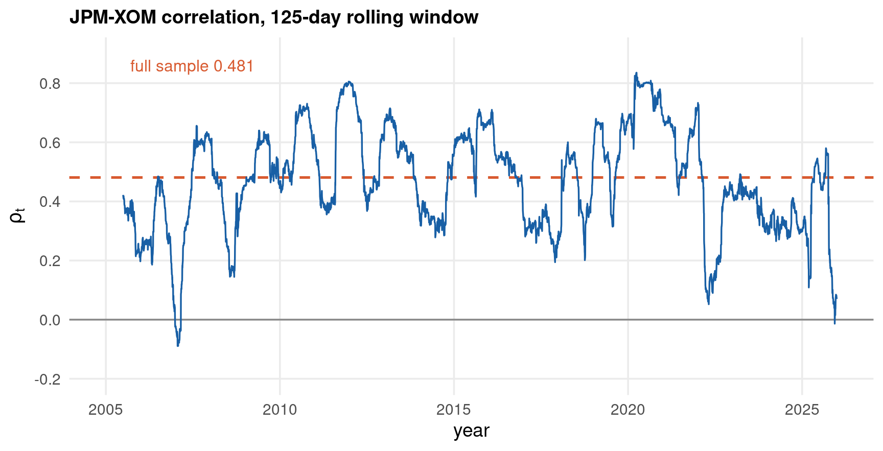
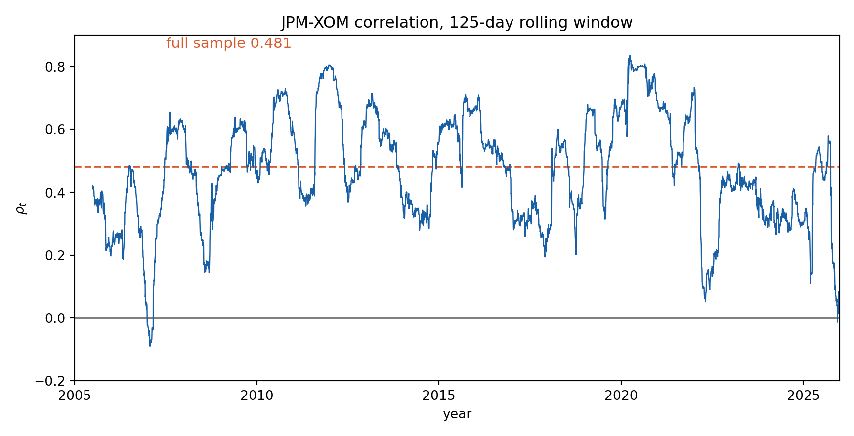
astavrak@uoi.gr · linkedin.com/in/astavrakoudis