Part 2 takes \(f\) degenerate and the integral disappears — that is logit, and it is the only case with a closed form. Part 3 weakens the error assumption as far as it can go while keeping the closed form. Part 4 gives it up entirely, and from there the econometrics is inseparable from the numerics: the estimator is only as good as the simulator, and the simulator is only as good as its draws.
This deck is about where choice probabilities come from and how to compute them, not about the industrial-organisation models built on top.
Companion decks own the neighbouring ground. Structural Estimation in Econometrics owns BLP demand and Rust’s dynamic discrete choice — both of which use the machinery built here without teaching it; Part 8 hands off to them explicitly. Moments-Based Structural Estimation owns common random numbers in the context of simulated moments; the same idea appears in Part 5 for a simulated likelihood, and seeing it twice in two settings is deliberate. Numerical Applications owns quadrature, BFGS and the hand-coded logit MLE that Part 2 repeats on purpose — a student taking only this deck should not have to go and get it.
Those decks ask what does this market look like? This deck asks given a random-utility model, what is the probability that this person chooses this alternative — and how do I compute it when the integral has no closed form?
import numpy as np # arrays; the hand-coded GHK simulatorimport pandas as pd # long-format choice dataimport scipy.stats as st # normal CDF/PDF inside GHKfrom scipy.optimize import minimize # every hand-coded likelihoodfrom scipy.stats import qmc # Halton and Sobol sequencesfrom xlogit import MultinomialLogit, MixedLogit # MNL and mixed logit by MSLimport matplotlib.pyplot as plt # all figures
* All native to Stata SE - no installation needed:cmset id alt // declare the choice-model data structure, oncecmclogit // conditional (McFadden) logitasclogit // alternative-specific conditional logitmlogit// multinomial logit on individual-specific regressorsnlogit// nested logit, with nlogitgen / nlogittreecmmixlogit // mixed logit by maximum simulated likelihoodcmxtmixlogit // panel mixed logitcmmprobit // multinomial probit by GHKmargins // elasticities and average marginal effectsmata: optimize() // the hand-written GHK simulator of Part 4
Stata is the strongest of the three languages for this material.nlogit, cmmixlogit and cmmprobit are native, fast and well documented, and cmset declares the data structure once so every later command inherits it. This series has been honest where Stata is weak — copulas, Bayesian computation, dynamic programming — and it should be equally honest here.
Data & Provenance
Every dataset is written once by dchoice-data.R and only read by the deck.
File
Content
Source
dchoice-mode.csv
Intercity travel mode choice, long format: id, alt, choice, cost, ivt, ovt, freq, income
mlogit::ModeCanada — real revealed-preference data
dchoice-mixed.csv
1000 individuals × 4 alternatives; one normal and one lognormal random coefficient, both known
simulated, seed 14159
dchoice-probit.csv
4-alternative multinomial probit with a known, non-diagonal error covariance
simulated, seed 14159
Why a CSV and not a native load. This series prefers native package loads. ModeCanada ships in R’s mlogit and has no Python or Stata equivalent, which is exactly the stated exception for R-only packages. It is extracted once to CSV so all three languages analyse the identical file.
One long format for three libraries. Choice data is per-alternative, and R’s dfidx, Python’s xlogit and Stata’s cmset each want their own object — built from the same long file. Every dataset here is a complete id × alt rectangle with exactly one chosen alternative per decision-maker.
A decision-maker \(n\) faces a set of alternatives and picks exactly one. We observe the choice, the attributes of every alternative — chosen or not — and some characteristics of the chooser. We want the probability
\[P_{ni} = \Pr(\text{person } n \text{ chooses alternative } i)\]
as a function of those attributes, and we want it to mean something economically rather than merely fit.
Three features make this different from a regression on a continuous outcome:
the outcome is mutually exclusive and exhaustive — the probabilities must sum to one
the regressors vary across alternatives, not only across people
the interesting quantity is usually a substitution pattern, not a coefficient
Regress a 0/1 choice indicator on attributes and three things break, in increasing order of seriousness.
It leaves the unit interval. Fitted values below 0 and above 1 are not awkward, they are meaningless, and they arrive exactly where the data is thinnest.
It cannot enforce adding-up. With \(J\) separate linear probabilities nothing makes \(\sum_j \hat P_{nj} = 1\) hold, so the fitted object is not a distribution over choices.
It has no substitution pattern. This is the real objection. A choice model must answer if this alternative gets worse, where do those people go? The LPM answers “nowhere in particular”, because it never modelled the comparison.
The LPM is not a bad approximation to a choice model. It is a model of something else — a conditional mean — that happens to be numerically close in the middle of the data and structurally silent about the question we are asking.
Model the comparison, not the outcome. Give every alternative a utility, let the decision-maker take the largest, and accept that the analyst cannot see all of it. The probability then comes from the part we cannot see.
That single move — utility we observe, plus utility we do not — generates logit, probit, nested logit and mixed logit as special cases, and it is the reason all four share one formula.
\(V_{nj} = V(x_{nj}, s_n; \beta)\) is the representative utility, almost always linear in parameters, \(V_{nj} = \beta' x_{nj}\). The choice is
\[y_n = i \iff U_{ni} \ge U_{nj} \quad \text{for all } j\]
This is the point most often misread, so it is worth being blunt.
\(\varepsilon_{nj}\) is not a mistake, a shock to the person, or irrationality. The decision-maker knows their own utility exactly and maximises it without error. \(\varepsilon_{nj}\) is the part of that utility the analyst does not observe — unmeasured attributes, unmeasured taste, measurement error in \(x\).
The randomness is a statement about the econometrician’s information, not the agent’s.
Consequence: the distribution of \(\varepsilon\) is an assumption about what we failed to measure. Choosing it is a modelling decision with economic content, not a convenience. Parts 3 and 4 are entirely about the cost of choosing badly.
Because \(\varepsilon_n = (\varepsilon_{n1},\dots,\varepsilon_{nJ})\) is unobserved, the choice is a random event with
The indicator carves out the region where alternative \(i\) wins. Only \(J-1\) differences matter, so the integral is genuinely \((J-1)\)-dimensional. Every model in this deck is a statement about how to evaluate it:
\(f(\varepsilon)\)
resulting model
the integral
iid type-I extreme value
logit
closed form
GEV
nested logit
closed form
multivariate normal
probit
no closed form
EV1, but \(\beta\) itself random
mixed logit
no closed form
Once tastes are allowed to vary across people, the two rows without a closed form merge into one expression — the expression this deck is built around:
Part 2 makes \(f\) degenerate — all the mass at one \(\beta\) — and the integral vanishes, leaving the logit formula. Part 3 keeps a closed form by weakening the independence of the errors instead. Part 4 abandons closed forms entirely. Parts 5 and 6 are about computing the integral honestly once it has none.
From Part 4 onward the estimator and the numerical method stop being separable. A simulated log-likelihood is not “the likelihood, approximately” — it is a different objective function, with its own bias, noise and smoothness. Three consequences drive the rest of the deck:
an unbiased probability simulator gives a biased log-likelihood, because \(\log\) is nonlinear
a simulator that is not smooth in \(\theta\) breaks the optimiser before it breaks the estimate
the draws must be held fixed across iterations, or the objective moves while you climb it
Add any constant \(c\) to every alternative’s utility for a given person:
\[U_{nj}^{*} = U_{nj} + c \quad \text{for all } j\]
The ranking is unchanged, so the observed choice is unchanged, so the likelihood is unchanged. Nothing in the data can distinguish \(U\) from \(U^{*}\).
Only utility differences are identified. The level is not a parameter of the model; it is a gauge freedom.
Alternative-specific constants. Only \(J-1\) of them are estimable. One alternative is the base and its constant is set to zero. That is a normalisation, not a hypothesis — it changes the reported numbers, not the fit.
Person-specific regressors need alternative-specific coefficients. A variable like income does not vary over \(j\), so \(\beta' s_n\) cancels from every difference. It can only enter interacted with the alternative, giving \(J-1\) coefficients. That is why income appears three times, not once, in every ModeCanada table in this deck.
The base alternative must be pinned deliberately in every language. R’s reflevel=, Stata’s basealternative() and Python’s base_alt= must agree, or three correct fits will print three different-looking tables.
A trap that is live in this deck. Give xlogit a string alternative column and it returns the coefficient vector relative to one base while printing the labels of another. The log-likelihood is right; the names are wrong. Every Python tab here indexes on the numeric altnum for exactly this reason.
Again the ranking, the choice and the likelihood are unchanged. So \(\beta\) is identified only relative to the scale of the error. What the data pins down is the ratio
\[\frac{\beta}{\sigma_\varepsilon}\]
and never \(\beta\) and \(\sigma_\varepsilon\) separately.
Coefficients are not comparable across models. Logit fixes \(\text{Var}(\varepsilon) = \pi^2/6\) by assumption; probit fixes something else. A logit coefficient larger than a probit coefficient on the same data is usually reporting a different scale, not a different effect. The familiar logit/probit factor of roughly \(\pi/\sqrt{3} \approx 1.81\) is exactly this.
Where the 1.81 comes from
Only the difference of two errors enters a binary choice, so compare the models on that difference rather than on \(\varepsilon\) itself.
Logit. Each \(\varepsilon_j\) is type-I extreme value with variance \(\pi^2/6\). The two are independent, so
The ratio is a property of the two conventions, not of the data — it would appear even if both models fitted perfectly.
In practice the observed ratio is usually nearer \(1.6\), because the distributions differ in the tails and the fitted probabilities are not identical.
Ratios such as willingness to pay, and all elasticities, are unaffected: the \(\sigma_\varepsilon\) cancels.
Ratios are safe; levels are not. Any ratio of two coefficients cancels \(\sigma_\varepsilon\) and is identified. This is why willingness to pay,
\[\text{WTP} = \frac{\partial V / \partial x}{\partial V / \partial \text{cost}}\]
is comparable across models when coefficients are not. Part 2 estimates it and Part 7 reports it as the policy number.
Elasticities are safe too, for the same reason — they are built from probabilities, which are scale-free.
Rule of thumb for reading any discrete-choice table: compare ratios, elasticities and predicted probabilities across specifications; never compare raw coefficients.
Every model in this deck is one choice of \(f(\varepsilon)\), and each choice buys a closed form or a substitution pattern, but rarely both.
assumption on \(\varepsilon\)
model
substitution
cost
iid EV1 across \(j\)
logit
proportional (IIA)
too restrictive
GEV — correlated within nests
nested logit
free between nests
tree must be assumed
\(N(0,\Sigma)\), \(\Sigma\) free
multinomial probit
fully free
no closed form
EV1 + random \(\beta\)
mixed logit
fully free
no closed form
The first row is the workhorse and the whole reason the other three exist. The independence in “iid” is what forces proportional substitution: if the unobserved parts of two alternatives are independent, nothing makes two similar alternatives compete more closely with each other than with a third.
Rows 2–4 are three different ways of letting unobservables be correlated across alternatives:
nested logit correlates them within an analyst-specified group
probit correlates them freely, through \(\Sigma\)
mixed logit correlates them through shared tastes — two alternatives loading on the same random coefficient move together
McFadden and Train (2000) proved that the last row can approximate any random utility model arbitrarily closely, given a suitable mixing distribution. That is why mixed logit is the destination of this deck — and why Part 6 spends its time on how to compute it rather than on whether to use it.
It is chosen for tractability, but it is not eccentric: EV1 is the limiting distribution of a maximum of many independent draws, and utility is a maximum over unobserved attributes. Its variance is fixed at \(\pi^2/6\), which is the scale normalisation of Part 1 made concrete.
Condition on \(\varepsilon_{ni}\). Alternative \(i\) wins when every other \(\varepsilon_{nj}\) is small enough:
Integrate \(\varepsilon_{ni}\) out. Substituting \(t = e^{-\varepsilon_{ni}}\) turns the whole thing into \(\int_0^\infty e^{-t \sum_j e^{-(V_{ni}-V_{nj})}}dt\), which is elementary:
Each term of the Hessian is a probability-weighted covariance matrix, hence negative semi-definite, and a sum of negative semi-definite matrices is negative semi-definite. So \(\ell(\beta)\) is globally concave.
The two-line proof
Fix a decision-maker \(n\) and treat the probabilities \(P_{nj}\) as weights on the regressor vectors \(x_{nj}\), with \(\bar{x}_n = \sum_j P_{nj} x_{nj}\) the weighted mean. That decision-maker’s block of the Hessian is
Take any vector \(c\) and form the quadratic form:
\[ c' H_n c \;=\; -\sum_j P_{nj}\,\big[c'(x_{nj} - \bar{x}_n)\big]^2 \;\le\; 0 \]
The bracket is a scalar, so its square is non-negative; the weights \(P_{nj}\) are positive; the leading minus sign makes the whole expression non-positive. So \(H_n\) is negative semi-definite for every\(n\) and every \(\beta\), and \(H = \sum_n H_n\) inherits it.
Read \(H_n\) as minus a weighted covariance matrix of the regressors across alternatives — that is exactly what it is.
It is strictly negative definite unless some \(c\) makes \(c'x_{nj}\) identical across all \(j\), for all \(n\). That is precisely the collinearity case: a regressor constant across alternatives has already dropped out of the utility differences.
So a singular Hessian is a data diagnosis, not an optimiser failure — which is why non-convergence in a logit means perfect prediction or collinearity.
This is not a technicality. It means:
any interior maximum is the maximum — no local optima, no multistart
Newton–Raphson from any starting point converges, usually in fewer than 10 iterations
starting values do not matter, so nobody reports them
non-convergence signals a data problem — perfect prediction or collinearity — not an optimiser problem
Remember this slide when you reach Part 6. The simulated log-likelihood of a mixed logit is not concave, starting values matter enormously, and “it did not converge” stops being diagnostic. Every convenience listed above is a property of this model only.
The hand-coded Newton–Raphson and BFGS machinery behind the next slide is developed in the companion deck Numerical Applications for Economics and Econometrics. It is repeated here rather than cited away, because a student taking only this deck needs to see the score and Hessian above turn into code.
Code — Logit MLE by Hand
Three implementations of the same estimator, each using the analytic score and Hessian from the previous slide. All three must return the identical log-likelihood; that is the point of the slide.
Code
md <-read.csv("../data/dchoice-mode.csv")md <- md[order(md$id, md$altnum), ]nalt <-4# design matrix: 3 ASCs (car is base), 4 generic attributes, 3 income slopesd1 <-as.numeric(md$altnum ==1) # traind2 <-as.numeric(md$altnum ==2) # aird3 <-as.numeric(md$altnum ==3) # busZ <-cbind(d1, d2, d3, md$freq, md$cost, md$ivt, md$ovt, d1 * md$income, d2 * md$income, d3 * md$income)colnames(Z) <-c("asc_train", "asc_air", "asc_bus", "freq", "cost", "ivt","ovt", "inc_train", "inc_air", "inc_bus")y <- md$choice# choice probabilities, one column per decision-makerprobs <-function(th) { V <-matrix(Z %*% th, nrow = nalt) V <-sweep(V, 2, apply(V, 2, max)) # subtract max for numerical safety P <-exp(V)sweep(P, 2, colSums(P), "/")}negll <-function(th) -sum(log(colSums(probs(th) *matrix(y, nrow = nalt))))negscore <-function(th) -as.vector(t(Z) %*% (y -as.vector(probs(th))))# Hessian: minus the sum of within-decision-maker covariance matriceshessian <-function(th) { P <-as.vector(probs(th)) H <-matrix(0, ncol(Z), ncol(Z))for (n inseq_len(nrow(md) / nalt)) { k <- ((n -1) * nalt +1):(n * nalt) Zn <- Z[k, , drop =FALSE] pn <- P[k] zb <-crossprod(Zn, pn) H <- H - (crossprod(Zn * pn, Zn) -tcrossprod(zb)) } H}fit <-optim(rep(0, ncol(Z)), negll, gr = negscore, method ="BFGS",control =list(maxit =2000, reltol =1e-15))se <-sqrt(diag(solve(-hessian(fit$par))))cat("log-likelihood =", format(-fit$value, digits =10), "\n")print(data.frame(coef =round(fit$par, 6), se =round(se, 6),row.names =colnames(Z)))
quietly import delimited "../data/dchoice-mode.csv", clearquietlydestring_all, replacesort id altnumquietlygen asc_train = (altnum == 1)quietlygen asc_air = (altnum == 2)quietlygen asc_bus = (altnum == 3)quietlygen inc_train = asc_train * incomequietlygen inc_air = asc_air * incomequietlygen inc_bus = asc_bus * incomemata:// value and analytic gradient; nalt is passed in so J() stays availablevoid mnl_d1(todo, theta, Z, y, nalt, lnf, g, H){realmatrixV, PrealcolvectorpV = colshape(Z * theta', nalt)V = V :- rowmax(V) P = exp(V); P = P :/ rowsum(P)p = vec(P') lnf = sum(log(rowsum(P :* colshape(y, nalt))))if (todo >= 1) g = (y - p)' * Z}// minus the sum of within-decision-maker covariance matricesrealmatrix mnl_hess(realrowvector theta, realmatrix Z, realcolvectory,realscalar nalt){realmatrixV, P, H, Znrealcolvectorp, pn, zbrealscalar n, ncV = colshape(Z * theta', nalt); V = V :- rowmax(V) P = exp(V); P = P :/ rowsum(P)p = vec(P'); nc = rows(Z) / nalt H = J(cols(Z), cols(Z), 0)for (n = 1; n <= nc; n++) { Zn = Z[((n-1)*nalt+1)::(n*nalt), .] pn = p[((n-1)*nalt+1)::(n*nalt)] zb = Zn' * pn H = H - (Zn' * (Zn :* pn) - zb * zb') }return(H)}Z = st_data(., "asc_train asc_air asc_bus freq cost ivt ovt inc_train inc_air inc_bus")y = st_data(., "choice")S = optimize_init()optimize_init_evaluator(S, &mnl_d1())optimize_init_evaluatortype(S, "d1")optimize_init_argument(S, 1, Z)optimize_init_argument(S, 2, y)optimize_init_argument(S, 3, 4)optimize_init_params(S, J(1, cols(Z), 0))optimize_init_technique(S, "nr")optimize_init_tracelevel(S, "none")b = optimize(S)printf("log-likelihood = %12.6f\n\n", optimize_result_value(S))se = sqrt(diagonal(invsym(-mnl_hess(b, Z, y, 4))))nm = ("asc_train", "asc_air", "asc_bus", "freq", "cost", "ivt", "ovt","inc_train", "inc_air", "inc_bus")printf("%-11s %12s %11s\n", "", "coef", "se")for (i = 1; i <= cols(b); i++) printf("%-11s %12.6f %11.6f\n", nm[i], b[i], se[i])end
------------------------------------------------- mata (type end to exit) ----------------------------------------------
: // value and analytic gradient; nalt is passed in so J() stays available
: void mnl_d1(todo, theta, Z, y, nalt, lnf, g, H)
> {
>     real matrix V, P
>     real colvector p
>     V = colshape(Z * theta', nalt)
>     V = V :- rowmax(V)
>     P = exp(V); P = P :/ rowsum(P)
>     p = vec(P')
>     lnf = sum(log(rowsum(P :* colshape(y, nalt))))
>     if (todo >= 1) g = (y - p)' * Z
> }
note: argument H unused.

:
: // minus the sum of within-decision-maker covariance matrices
: real matrix mnl_hess(real rowvector theta, real matrix Z, real colvector y,
>                      real scalar nalt)
> {
>     real matrix V, P, H, Zn
>     real colvector p, pn, zb
>     real scalar n, nc
>     V = colshape(Z * theta', nalt); V = V :- rowmax(V)
>     P = exp(V); P = P :/ rowsum(P)
>     p = vec(P'); nc = rows(Z) / nalt
>     H = J(cols(Z), cols(Z), 0)
>     for (n = 1; n <= nc; n++) {
>         Zn = Z[((n-1)*nalt+1)::(n*nalt), .]
>         pn = p[((n-1)*nalt+1)::(n*nalt)]
>         zb = Zn' * pn
>         H  = H - (Zn' * (Zn :* pn) - zb * zb')
>     }
>     return(H)
> }
note: argument y unused.

:
: Z = st_data(., "asc_train asc_air asc_bus freq cost ivt ovt inc_train inc_air inc_bus")

: y = st_data(., "choice")

:
: S = optimize_init()

: optimize_init_evaluator(S, &mnl_d1())

: optimize_init_evaluatortype(S, "d1")

: optimize_init_argument(S, 1, Z)

: optimize_init_argument(S, 2, y)

: optimize_init_argument(S, 3, 4)

: optimize_init_params(S, J(1, cols(Z), 0))

: optimize_init_technique(S, "nr")

: optimize_init_tracelevel(S, "none")

: b = optimize(S)

:
: printf("log-likelihood = %12.6f\n\n", optimize_result_value(S))
log-likelihood = -1930.565158


: se = sqrt(diagonal(invsym(-mnl_hess(b, Z, y, 4))))

: nm = ("asc_train", "asc_air", "asc_bus", "freq", "cost", "ivt", "ovt",
>       "inc_train", "inc_air", "inc_bus")

: printf("%-11s %12s %11s\n", "", "coef", "se")
                    coef          se

: for (i = 1; i <= cols(b); i++) printf("%-11s %12.6f %11.6f\n", nm[i], b[i], se[i])
asc_train       2.192521    0.284731
asc_air         2.051572    0.494849
asc_bus        -1.624869    0.713767
freq            0.093101    0.004763
cost           -0.044963    0.003938
ivt            -0.009986    0.000751
ovt            -0.042912    0.002830
inc_train      -0.009484    0.003145
inc_air         0.027276    0.003683
inc_bus        -0.059455    0.017924

: end
------------------------------------------------------------------------------------------------------------------------
Code — Off the Shelf
The same model through each language’s production command. The coefficients and the log-likelihood must reproduce the hand-coded slide to the printed digit.
Code
library(mlogit)md <-read.csv("../data/dchoice-mode.csv")md$alt <-factor(md$alt, levels =c("train", "air", "bus", "car"))MC <-dfidx(md, idx =c("id", "alt"), choice ="choice")# freq/cost/ivt/ovt are alternative-specific with a generic coefficient;# income is person-specific, so it gets one coefficient per alternativemnl <-mlogit(choice ~ freq + cost + ivt + ovt | income,data = MC, reflevel ="car")summary(mnl)
quietly import delimited "../data/dchoice-mode.csv", clearquietlydestring_all, replace* cmset declares the choice structure once; later commands inherit itcmset id altnumcmclogit choice freq cost ivt ovt, casevars(income) basealternative(4) nolog
     Case ID variable: id
Alternatives variable: altnum


Conditional logit choice model                 Number of obs      =     11,116
Case ID variable: id                           Number of cases    =       2779

Alternatives variable: altnum                  Alts per case: min =          4
                                                              avg =        4.0
                                                              max =          4

                                                  Wald chi2(7)    =     984.07
Log likelihood = -1930.5652                       Prob > chi2     =     0.0000

------------------------------------------------------------------------------
      choice | Coefficient  Std. err.      z    P>|z|     [95% conf. interval]
-------------+----------------------------------------------------------------
altnum       |
        freq |   .0931011   .0047625    19.55   0.000     .0837668    .1024355
        cost |  -.0449629   .0039382   -11.42   0.000    -.0526817   -.0372442
         ivt |   -.009986   .0007511   -13.29   0.000    -.0114582   -.0085138
         ovt |  -.0429118   .0028296   -15.17   0.000    -.0484577   -.0373658
-------------+----------------------------------------------------------------
1            |
      income |  -.0094841   .0031453    -3.02   0.003    -.0156489   -.0033193
       _cons |   2.192521   .2847307     7.70   0.000     1.634459    2.750582
-------------+----------------------------------------------------------------
2            |
      income |    .027276   .0036827     7.41   0.000      .020058    .0344939
       _cons |   2.051572   .4948493     4.15   0.000     1.081685    3.021459
-------------+----------------------------------------------------------------
3            |
      income |  -.0594545   .0179241    -3.32   0.001    -.0945851   -.0243238
       _cons |  -1.624878   .7137659    -2.28   0.023    -3.023834   -.2259227
-------------+----------------------------------------------------------------
4            |  (base alternative)
------------------------------------------------------------------------------
base_alt and string alternatives do not mix in xlogit. Passing alts=df["alt"], base_alt="car" returns the coefficient vector relative to bus, printed under air/bus/train labels. The log-likelihood is correct, so nothing looks wrong. Indexing on altnum with base_alt=4 reproduces R and Stata to six decimals.
A logit coefficient is a derivative of utility, measured in an arbitrary scale unit. It is not a derivative of the probability, and it is not comparable across models. What can be reported are the derivatives of probabilities.
The own-derivative for a generic-coefficient attribute is
Read the second formula carefully. The cross-elasticity \(E_{ij}\)does not depend on \(i\). Raise the cost of air travel and every other mode’s share rises by the same percentage — train, bus and car alike. That is not an approximation or a small-sample artefact; it is an algebraic identity of the logit model, and it is the next slide.
Own- and Cross-Elasticities
Evaluated at a representative decision-maker: every attribute at its alternative-specific sample mean, income at the sample mean. Entry \([i,j]\) is the elasticity of alternative \(i\)’s share with respect to alternative \(j\)’s cost.
The denominator cancels. The odds of \(i\) against \(k\) depend on \(i\) and \(k\) alone, and on nothing else in the choice set — hence independence from irrelevant alternatives. Adding, removing or worsening a third alternative leaves those odds untouched.
IIA is a modelling assumption with real content, and sometimes the content is right:
it makes the model robust to the choice set — estimate on a subset of alternatives and the parameters are still consistent, which is how anyone estimates a model over thousands of alternatives
it makes forecasting to new alternatives possible at all, since a new option’s share follows from its attributes alone
with genuinely distinct alternatives and rich enough \(V\), proportional substitution is often a reasonable approximation
The sampling-of-alternatives property is not a curiosity. It is why McFadden’s logit could be applied to residential location choice over an enormous choice set in 1978, and why it remains the only tractable option in many large problems.
IIA fails whenever two alternatives share unobserved attributes — when they are closer substitutes for each other than for the rest. The elasticity table two slides back showed the mechanism: raising air fares pushes travellers to train, bus and car in exactly equal proportion, which is not how anyone believes travellers behave.
The canonical counterexample is Part 3’s opening slide, and the rest of the deck is the set of repairs:
nested logit — correlate the unobservables inside analyst-chosen groups
probit — let \(\Sigma\) be free
mixed logit — correlate them through shared random tastes
Part 1 established that \(\beta\) is identified only up to the scale of the error, so a coefficient means nothing on its own. A ratio of two coefficients has the scale cancel:
\[\text{WTP}_x = \frac{\partial V / \partial x}{\partial V / \partial \text{cost}}
= \frac{\beta_x}{\beta_{\text{cost}}}\]
measured in currency per unit of \(x\). For a travel-time coefficient this is the value of travel time savings — the number that goes into a cost–benefit appraisal, and the reason transport agencies estimate these models at all.
WTP is a nonlinear function of two estimates, so its variance comes from the delta method. With \(r = \beta_x / \beta_c\) and gradient
the standard error is \(\sqrt{g' \, \text{Var}(\hat\beta_x, \hat\beta_c)\, g}\).
The delta method is a first-order approximation and it is at its worst for ratios whose denominator is imprecise. When \(\beta_{\text{cost}}\) is close to zero relative to its standard error the WTP distribution is heavy-tailed and the symmetric interval below understates the uncertainty badly. The bootstrap and Fieller’s method are the standard alternatives — see the companion deck Bootstrap Methods in Econometrics.
Code
b <-coef(mnl); V <-vcov(mnl)for (v inc("ivt", "ovt")) { r <- b[v] / b["cost"] # CAD per minute g <-c(1/ b["cost"], -b[v] / b["cost"]^2) # delta-method gradient se <-sqrt(t(g) %*% V[c(v, "cost"), c(v, "cost")] %*% g)cat(sprintf("%s: %7.4f CAD/hour se %6.4f 95%% CI [%7.4f, %7.4f]\n", v, 60* r, 60* se, 60* (r -1.96* se), 60* (r +1.96* se)))}
ivt: 13.3256 CAD/hour   se 1.7895   95% CI [ 9.8182, 16.8330]
ovt: 57.2629 CAD/hour   se 6.2780   95% CI [44.9581, 69.5677]
Code
quietly import delimited "../data/dchoice-mode.csv", clearquietlydestring_all, replacequietly cmset id altnumquietly cmclogit choice freq cost ivt ovt, casevars(income) basealternative(4)* nlcom applies the delta method to the ratio, then converts to CAD per hournlcom (VTTS_ivt: 60 * _b[ivt] / _b[cost]) (VTTS_ovt: 60 * _b[ovt] / _b[cost])
In-vehicle time is worth about 13 CAD/hour to these travellers; out-of-vehicle time — waiting, transferring, walking — is worth roughly four times more per minute. That gap is one of the most robust findings in transport economics, and it is invisible in the raw coefficients.
Part 3 — Breaking IIA
Nested logit, GEV, and the tests you should not over-trust
Now the operator paints half the fleet red. The red bus is identical to the blue bus in every respect except colour, which nobody cares about, so \(V_{\text{red}} = V_{\text{blue}}\).
What should happen: the bus share stays at \(\tfrac12\) and splits between the two colours. What logit says: three alternatives with equal \(V\), so
Painting buses took a sixth of the market away from cars.
The logit answer is not a bug in the arithmetic — it is IIA doing exactly what Part 2 said it does. The odds of car against blue bus are \(1{:}1\) before and \(1{:}1\) after, which is what IIA guarantees. The error is in the level.
The mechanism is the independence assumption. Logit treats the red bus as a genuinely new option drawing on independent unobservables, when in truth \(\varepsilon_{\text{red}}\) and \(\varepsilon_{\text{blue}}\) are the same unobservable — anyone who dislikes buses dislikes both.
true answer
logit
car
0.500
0.333
blue bus
0.250
0.333
red bus
0.250
0.333
Put the two buses in a nest and let their unobservables be correlated. With a bus nest of dissimilarity \(\lambda\) and equal \(V\) throughout, the algebra gives a one-parameter family:
\(\lambda = 1\)is the logit model, and \(\lambda \to 0\) is perfect substitution within the nest. The whole of nested logit is the observation that this number does not have to be 1, and can be estimated.
Generalised extreme value keeps almost everything that makes logit work while dropping independence. Let \(G(y_1,\dots,y_J)\) be a function of \(y_j = e^{V_j}\) satisfying four conditions:
\(G \ge 0\) and homogeneous of degree one
\(G \to \infty\) as any \(y_j \to \infty\)
\(k\)-th cross partial derivatives non-negative for odd \(k\), non-positive for even \(k\)
Then \(\exp\!\left(-G(e^{-\varepsilon_1},\dots,e^{-\varepsilon_J})\right)\) is a valid joint CDF, and the resulting choice probability is
Keeps: a closed form. Every GEV model has choice probabilities expressible in elementary functions, so estimation is ordinary maximum likelihood with no simulation. That is the entire reason the class is interesting.
Buys: correlation between the unobserved components, and therefore substitution patterns that are not proportional.
GEV is where the closed form stops. Every model in Parts 4–6 gives it up, and pays for the freedom with simulation. Nested logit is the last stop before the integral becomes intractable — which is why it is still the workhorse whenever the analyst is confident about the tree.
Partition the \(J\) alternatives into \(K\) mutually exclusive nests \(B_1,\dots,B_K\). Alternatives inside a nest share unobserved components; alternatives in different nests do not. The probability factors into a choice of nest and a choice within nest:
\[P_{ni} = \underbrace{P_{n}(B_k)}_{\text{which nest}} \times
\underbrace{P_{n}(i \mid B_k)}_{\text{which alternative in it}}\]
Within the nest, an ordinary logit on utilities scaled by \(\lambda_k\):
\(I_{nk}\) is a log-sum-exponential, so it is a smooth maximum of the utilities in nest \(k\) — the expected utility a decision-maker gets from having that nest available, up to a constant.
That is its economic meaning, and it is why it appears again in welfare analysis as the log-sum measure of consumer surplus. The upper model does not see the individual alternatives inside a nest; it sees only “how attractive is this nest as a whole”, and the inclusive value is that summary.
\(\lambda_k\) controls the correlation of unobservables within nest \(k\):
and the implied joint CDF of the errors is \(\exp\{-G(e^{-\varepsilon_1},\dots,e^{-\varepsilon_J})\}\). Within a nest this is a Gumbel copula with dependence parameter \(1/\lambda_k\), whose Kendall correlation is \(1-\lambda_k\) and whose Pearson correlation of the underlying extreme-value marginals works out to
\(\lambda_k = 1\) gives correlation \(0\). The Gumbel copula degenerates to independence, \(G\) collapses to \(\sum_j y_j\), and the model is the logit of Part 2.
\(\lambda_k \to 0\) gives correlation \(\to 1\). The alternatives in the nest share their entire unobserved component, so they behave as one composite alternative — the red bus / blue bus answer.
\(\lambda_k > 1\) would require a correlation below zero, which this copula cannot produce. That is the analytic reason the restriction is \(\lambda_k \le 1\) and not merely a convention.
The same \(\lambda_k\) therefore does two jobs at once: it scales utilities inside the nest, and it is the dependence parameter. Estimating it is estimating how alike the analyst’s grouping really was.
For nested logit to be consistent with random utility maximisation for all values of the explanatory variables, the dissimilarity parameters must satisfy
This is not a numerical convenience. It comes from the GEV conditions: outside that range the implied \(G\) is not a valid generating function, the implied joint CDF is not a CDF, and the “probabilities” need not lie in \([0,1]\) for every configuration of \(V\).
\(\hat\lambda > 1\) is a specification failure, not a finding. Read in the correlation formula it would imply a negative correlation of unobservables within the nest — the alternatives you grouped together are less alike than alternatives in different nests. Usually it means the tree is upside down.
What to do, in order:
re-examine the tree; the grouping is probably wrong
try the alternative trees that theory also permits, and compare
consider that the substitution pattern may not be nested at all — Parts 4 and 6 exist for this
do not simply constrain \(\lambda = 1\) and report the logit as if nothing happened
Two slides from now this deck estimates a tree with \(\hat\lambda = 1.43\) — and that tree has the best log-likelihood of any tree tried. Fit is not the criterion. A model that fits well and violates RUM is not a better model; it is evidence that the nesting story is wrong.
A nest containing exactly one alternative has no within-nest choice to make. Its \(\lambda_k\) then multiplies an inclusive value equal to \(V_j/\lambda_k\), so
and \(\lambda_k\)cancels entirely — it is not identified and not estimable.
This matters practically: in the specification below, air sits alone in its nest, and Stata says so explicitly (“branch 1 of level 1 is degenerate and the associated dissimilarity parameter is not defined”). R reaches the same model by estimating a single shared \(\lambda\). The two are the same model, which is why the three tabs agree to six decimals.
Code — Nested Logit
Tree: air alone against a ground nest of train, bus and car. One dissimilarity parameter is estimable, and all three languages must agree on it.
Code
library(mlogit)md <-read.csv("../data/dchoice-mode.csv")md$alt <-factor(md$alt, levels =c("train", "air", "bus", "car"))MC <-dfidx(md, idx =c("id", "alt"), choice ="choice")# un.nest.el = TRUE estimates ONE lambda shared by both nests; with a# degenerate "fly" nest that is the only identified specificationnl <-mlogit(choice ~ freq + cost + ivt + ovt | income, data = MC,reflevel ="car",nests =list(fly ="air", ground =c("train", "bus", "car")),un.nest.el =TRUE)summary(nl)
Python has no maintained nested-logit library — pylogit, larch and biogeme are all unavailable here — so the tab hand-codes the likelihood. That is no loss: the inclusive value and the two-level factorisation are visible in the code rather than hidden in a package.
New variable type is generated with 2 groups
label list lb_type
lb_type:
           1 fly
           2 ground


Tree structure specified for the nested logit model

 type    N       altnum  N
----------------------------
 fly    2779 --- air    2779
 ground 8337 --- train  2779
              |- bus    2779
              +- car    2779
----------------------------
                Total  11116

N = number of observations at each level

note: branch 1 of level 1 is degenerate and the associated dissimilarity parameter [/type]fly_tau is not defined; see
      help nlogit for details.

Tree structure specified for the nested logit model

 type    N       altnum  N    k
---------------------------------
 fly    2779 --- air    2779 1039
 ground 8337 --- train  2779  463
              |- bus    2779   10
              +- car    2779 1267
---------------------------------
                Total  11116 2779

k = number of times alternative is chosen
N = number of observations at each level

RUM-consistent nested logit regression         Number of obs      =     11,116
Case variable: id                              Number of cases    =       2779

Alternative variable: altnum                   Alts per case: min =          4
                                                              avg =        4.0
                                                              max =          4

                                                  Wald chi2(7)    =     772.13
Log likelihood =  -1927.326                       Prob > chi2     =     0.0000

------------------------------------------------------------------------------
      choice | Coefficient  Std. err.      z    P>|z|     [95% conf. interval]
-------------+----------------------------------------------------------------
altnum       |
        freq |   .0920411   .0046016    20.00   0.000     .0830221    .1010601
        cost |  -.0413934   .0037033   -11.18   0.000    -.0486516   -.0341351
         ivt |   -.009276   .0007631   -12.16   0.000    -.0107717   -.0077803
         ovt |   -.039963   .0027745   -14.40   0.000    -.0454009    -.034525
------------------------------------------------------------------------------
altnum equations
------------------------------------------------------------------------------
train        |
      income |  -.0083889   .0026176    -3.20   0.001    -.0135194   -.0032585
       _cons |   2.091091   .2482963     8.42   0.000     1.604439    2.577743
-------------+----------------------------------------------------------------
air          |
      income |   .0273567   .0035751     7.65   0.000     .0203496    .0343637
       _cons |   1.567715   .4913113     3.19   0.001     .6047626    2.530668
-------------+----------------------------------------------------------------
bus          |
      income |  -.0480253   .0148923    -3.22   0.001    -.0772135    -.018837
       _cons |  -1.348081   .5879281    -2.29   0.022    -2.500399   -.1957631
-------------+----------------------------------------------------------------
car          |
      income |          0  (base)
       _cons |          0  (base)
------------------------------------------------------------------------------
dissimilarity parameters
------------------------------------------------------------------------------
/type        |
     fly_tau |          1   69803.77                     -136811.9    136813.9
  ground_tau |   .8053257   .0664615                      .6750635    .9355879
------------------------------------------------------------------------------
LR test for IIA (tau=1): chi2(2) = 6.48                   Prob > chi2 = 0.0392
Which Tree, and How You Defend It
Four candidate trees on the same data. The dissimilarity parameter and the log-likelihood are reported for each.
Against the MNL benchmark, tree 1 gives a likelihood-ratio statistic of \(2(-1927.3260 + 1930.5652) = 6.478\) on one degree of freedom, \(p \approx 0.011\). The direct test of \(\lambda = 1\) agrees: \(t = (0.8054 - 1)/0.0621 = -3.13\).
The fourth tree — everything except the car in one nest — fits best by a wide margin, better than the RUM-consistent trees by more than 7 log-likelihood points. It is also the one you cannot use.
\(\hat\lambda = 1.43\) is significantly above one (\(t = 4.03\)), so the model is not consistent with random utility maximisation. Reported as a headline result it would be indefensible, and no amount of fit repairs that.
This is the single most important slide in Part 3. Log-likelihood does not choose the tree. The admissible set is fixed first, by theory and by what the alternatives actually are; fit ranks models only inside that set.
The tree is an assumption, and it is not testable against all alternatives, so it has to be argued:
Substantive similarity. Group alternatives that share unobserved attributes — comfort, reliability, status. Ground modes share congestion exposure; air does not.
Institutional structure. Sequential decisions sometimes genuinely happen — choose a neighbourhood, then a house.
Robustness. Report the alternatives you tried, not just the winner. The table above is the honest form of that.
Prior literature. For ModeCanada, air-versus-ground is the specification used by Bhat (1995) and Koppelman & Wen (2000).
If no tree is defensible, that is a signal to move to Part 4 or Part 6, where the substitution pattern is estimated rather than assumed.
The idea exploits the property that made IIA attractive in the first place. If IIA holds, dropping alternatives from the choice set leaves the parameters consistent — less efficient, but consistent. If IIA fails, the restricted estimator is inconsistent, and the two disagree.
With \(\hat\beta_f\) from the full choice set and \(\hat\beta_r\) from a restricted subset, sharing \(K\) common parameters:
The middle term is a difference of covariance matrices, valid because \(\hat\beta_f\) is efficient under the null.
A likelihood-ratio alternative that avoids the covariance difference. Split the sample at random in two, estimate on each half, form a weighted combination of the two coefficient vectors, and compare the restricted-choice-set likelihood under that combination against its own maximum.
It has a genuine drawback that is rarely admitted: the statistic depends on the random split. Two analysts running it on the same data get different answers, and the same analyst gets a different answer on a different seed.
Both tests are known to behave badly, and this deck’s data shows it rather than asserting it.
\(\widehat{V}_r - \widehat{V}_f\)need not be positive definite in finite samples, so \(H\) can be negative — a \(\chi^2\) statistic that cannot occur under any distribution
the result depends on which alternative you drop, with no guidance on which to pick
power against realistic alternatives is low; Hausman & McFadden themselves were cautious
Small–Hsiao adds simulation noise from the split
Use these tests as diagnostics, not verdicts. A rejection is informative; a non-rejection is weak evidence of very little. Estimating a nested logit or a mixed logit and comparing substitution patterns directly is more persuasive than any IIA test.
Testing IIA — Code
Hausman–McFadden on ModeCanada, dropping one alternative at a time.
Code
# refit on a restricted choice set; mlogit drops the decision-makers# whose chosen alternative is no longer availablesub_bus <-mlogit(choice ~ freq + cost + ivt + ovt | income, data = MC,reflevel ="car", alt.subset =c("car", "train", "air"))sub_train <-mlogit(choice ~ freq + cost + ivt + ovt | income, data = MC,reflevel ="car", alt.subset =c("car", "air", "bus"))hmftest(mnl, sub_bus) # drop bushmftest(mnl, sub_train) # drop train
drop bus : chisq = -1.9237 df = 8 p = 1
drop train: chisq = -21.8488 df = 8 p = 1
Both statistics are NEGATIVE: the estimated variance difference
is not positive definite, so the test is uninformative here.
Code
import numpy as np, pandas as pdfrom scipy.optimize import minimizemd = pd.read_csv("../data/dchoice-mode.csv").sort_values(["id", "altnum"])def fit(sub_alts): d = md[md["altnum"].isin(sub_alts)].copy()# a decision-maker who chose an excluded alternative must leave the sample d = d[d.groupby("id")["choice"].transform("sum") ==1] nalt =len(sub_alts) cols, names = [], []for k in (1, 2, 3): # car (altnum 4) is the baseif k in sub_alts: cols.append((d["altnum"] == k).astype(float).values) names.append("asc_%d"% k)for v in ["freq", "cost", "ivt", "ovt"]: cols.append(d[v].values.astype(float)); names.append(v)for k in (1, 2, 3):if k in sub_alts: cols.append((d["altnum"] == k).astype(float).values * d["income"].values) names.append("inc_%d"% k) Z = np.column_stack(cols); y = d["choice"].values.astype(float)def probs(th): V = (Z @ th).reshape(-1, nalt); V = V - V.max(axis=1, keepdims=True) P = np.exp(V);return P / P.sum(axis=1, keepdims=True)def nll(th): return-np.log((probs(th) * y.reshape(-1, nalt)).sum(axis=1)).sum()def nsc(th): return-(Z.T @ (y - probs(th).ravel()))def hess(th): P = probs(th).ravel(); H = np.zeros((Z.shape[1],) *2)for n inrange(len(y) // nalt): Zn = Z[n*nalt:(n+1)*nalt]; pn = P[n*nalt:(n+1)*nalt] zb = Zn.T @ pn H -= (Zn.T * pn) @ Zn - np.outer(zb, zb)return H r = minimize(nll, np.zeros(Z.shape[1]), jac=nsc, method="BFGS", options={"maxiter": 2000, "gtol": 1e-10})return (dict(zip(names, r.x)), pd.DataFrame(np.linalg.inv(-hess(r.x)), index=names, columns=names))bf, Vf = fit([1, 2, 3, 4])out =""for drop, keep in [("bus", [1, 2, 4]), ("train", [2, 3, 4])]: br, Vr = fit(keep) common = [k for k in br if k in bf] diff = np.array([br[k] - bf[k] for k in common]) Vd = (Vr.loc[common, common] - Vf.loc[common, common]).values stat = diff @ np.linalg.pinv(Vd) @ diff out +="drop %-6s HM chi2 = %10.4f df = %d\n"% (drop, stat, len(common))out +="\nBoth statistics are NEGATIVE -- the variance difference is not\n"out +="positive definite, so the test is uninformative on this sample.\n"import sys; sys.stdout.write(out +"\n"); sys.stdout.flush()
drop bus    HM chi2 =    -1.9237   df = 8
drop train  HM chi2 =   -21.8502   df = 8

Both statistics are NEGATIVE -- the variance difference is not
positive definite, so the test is uninformative on this sample.

213
Code
quietly import delimited "../data/dchoice-mode.csv", clearquietlydestring_all, replacequietly cmset id altnumquietly cmclogit choice freq cost ivt ovt, casevars(income) basealternative(4)estimatesstore full* drop bus (altnum 3) from the choice set and refitquietly cmclogit choice freq cost ivt ovt if altnum != 3, /// casevars(income) basealternative(4)estimatesstore nobushausman nobus full, alleqs constant
                 ---- Coefficients ----
             |      (b)          (B)            (b-B)     sqrt(diag(V_b-V_B))
             |     nobus         full        Difference       Std. err.
-------------+----------------------------------------------------------------
altnum       |
        freq |    .0933897     .0931011        .0002885        .0005478
        cost |   -.0455422    -.0449629       -.0005792        .0006077
         ivt |    -.009922     -.009986        .0000639        .0000824
         ovt |   -.0427741    -.0429118        .0001376        .0002325
-------------+----------------------------------------------------------------
1            |
      income |   -.0093923    -.0094841        .0000918        .0000755
       _cons |    2.172276     2.192521       -.0202447        .0243524
-------------+----------------------------------------------------------------
2            |
      income |    .0271288      .027276       -.0001471        .0001327
       _cons |    2.102615     2.051572        .0510435        .0542206
------------------------------------------------------------------------------
                       b = Consistent under H0 and Ha; obtained from cmclogit.
        B = Inconsistent under Ha, efficient under H0; obtained from cmclogit.

Test of H0: Difference in coefficients not systematic

chi2(8) = (b-B)'[(V_b-V_B)^(-1)](b-B)
        = -1.92

Warning: chi2 < 0 ==> model fitted on these data
         fails to meet the asymptotic assumptions
         of the Hausman test; see suest for a
         generalized test.
All three languages return the same negative statistic, \(\chi^2 = -1.92\) dropping bus and \(-21.85\) dropping train. Stata prints the diagnosis itself: “chi2 < 0 ==> model fitted on these data fails to meet the asymptotic assumptions of the Hausman test”. The nested logit two slides back rejected IIA cleanly on the same data. That contrast is the argument for estimating a richer substitution pattern rather than testing the restrictive one.
Nothing else changes. The decision-maker still maximises utility and the choice probability is still the probability that alternative \(i\) wins.
What changes is everything the model can say. \(\Sigma\) has free off-diagonal elements, so any pattern of correlation between unobservables is representable, and therefore any substitution pattern is representable. No IIA, no tree, no assumption about which alternatives resemble which.
Nested logit made the analyst commit to a tree before estimating. Probit does not: the data decides which alternatives share unobservables.
For the simulated data in this Part, alternatives 2 and 3 were built as close substitutes, with
and everything else independent. This is the red bus / blue bus structure of Part 3, now written into the data generating process rather than assumed by the analyst. The question of the Part is whether we can get 0.7 back.
has no closed form for \(J > 2\). There is no algebraic manipulation that resolves it, and there never will be. From here on, the choice probability must be computed numerically, and the way it is computed becomes part of the estimator.
Difference the system with respect to the chosen alternative \(i\). Let \(\tilde{\varepsilon}_j = \varepsilon_{nj} - \varepsilon_{ni}\) and \(\Delta_j = V_{nj} - V_{ni}\) for the \(J-1\) alternatives \(j \ne i\). Then
where \(M_i\) is the \((J-1) \times J\) differencing matrix. This is a multivariate normal orthant probability in \(J-1\) dimensions: the mass of a correlated normal over a rectangular region.
The integral has no closed form. For \(J-1 = 1\) it is \(\Phi(\cdot)\). For \(J-1 = 2\) there are accurate series. Beyond that, numerical work is unavoidable.
\(\Omega_i\) changes with the chosen alternative. Each decision-maker’s integral is over a different covariance matrix, because differencing is with respect to whichever alternative they chose. A method that is fast for one \(\Omega\) must be fast for all of them, and it must be re-run at every iteration of the optimiser, for every decision-maker.
Count the work. A likelihood evaluation needs \(N\) orthant probabilities in \(J-1\) dimensions. The optimiser needs hundreds of likelihood evaluations. Any method costing more than a few microseconds per probability is unusable, which rules out almost everything that is accurate.
Gaussian quadrature is the right tool for a smooth low-dimensional integral, and the companion deck Numerical Applications for Economics and Econometrics develops it properly. Its problem here is arithmetic, not accuracy.
A product rule with \(m\) nodes per dimension costs \(m^{J-1}\) function evaluations:
\(J\)
dimensions
\(m = 10\)
\(m = 20\)
3
2
100
400
4
3
1 000
8 000
5
4
10 000
160 000
8
7
\(10^{7}\)
\(1.3 \times 10^{9}\)
11
10
\(10^{10}\)
\(1.0 \times 10^{13}\)
Multiply the right-hand column by \(N\) decision-makers and by several hundred optimiser iterations. Quadrature is finished somewhere around \(J = 5\).
The curse of dimensionality is the famous objection, but there is a second one that matters just as much. Quadrature rules earn their fast convergence on smooth integrands. The integrand here is a normal density multiplied by an indicator function — it is discontinuous across the boundary of the acceptance region.
Polynomial-based rules approximate discontinuities badly, so the theoretical error bounds do not apply, and the practical accuracy is far worse than the node count suggests.
Monte Carlo error is \(O(R^{-1/2})\)regardless of dimension. It does not care that the region is an awkward polytope, and it does not care whether the integrand is smooth.
That is the trade: quadrature is far more accurate in low dimensions and unusable in high ones; simulation is mediocre everywhere and therefore usable everywhere. Part 5 is about making the mediocre part less mediocre.
Part 1 said only differences matter and only relative scale is identified. Applied to \(\Sigma\), this is severe. \(\Sigma\) has \(J(J+1)/2\) distinct elements, but the data can only ever speak about
\[\Omega = M \Sigma M'\]
for a differencing matrix \(M\), and only up to scale. The count:
\[\underbrace{\frac{J(J+1)}{2}}_{\text{elements of } \Sigma}
\ \longrightarrow\
\underbrace{\frac{J(J-1)}{2} - 1}_{\text{identified}}\]
For \(J = 4\): ten parameters in \(\Sigma\), but only five identified.
The simulated data has unit variances and one non-zero correlation:
The 0.7 in \(\Sigma\) appears as 0.85 in the differenced correlation, and the zeros appear as 0.5. Neither is a mistake: differencing induces correlation even between independent errors, because they share the subtracted term.
This is why MNP output is hard to read. A package reports the differenced, scale-normalised covariance — and every package normalises differently. Compare differenced correlations, predicted probabilities and elasticities across packages; never compare raw \(\Sigma\) entries.
Two restrictions must be imposed, and every implementation picks its own:
location — difference with respect to a base alternative (basealternative() in Stata)
scale — fix one variance of the differenced system (scalealternative() in Stata)
The estimation below sidesteps the reading problem in the Python tab by fixing unit variances and estimating the single correlation that generated the data. That is a restriction, it is stated as one, and it makes the answer directly comparable with the truth.
Named for Geweke, Hajivassiliou and Keane, who arrived at it independently. The naive approach — draw \(\varepsilon\) from \(N(0,\Omega)\) and count how often the inequalities hold — is a disaster: it is a frequency estimator, so it is zero whenever no draw lands in the region, and \(\log 0\) destroys the likelihood. It is also a step function of \(\theta\), so no gradient exists.
GHK never rejects a draw. It factors the orthant probability into a product of one-dimensional normal probabilities, each of which is computed exactly, and simulates only the conditioning.
Write \(\Omega = LL'\) with \(L\) lower triangular, so \(\tilde\varepsilon = Lz\) with \(z \sim N(0,I)\). The event \(\tilde\varepsilon < -\Delta\) becomes a sequence of conditions on \(z\), each involving only the \(z\)’s already drawn:
Step 1.\(\ell_{11} z_1 < -\Delta_1\), so \(z_1 < -\Delta_1/\ell_{11}\). This happens with the exact probability
Unbiased.\(\mathbb{E}[\hat P_{ni}] = P_{ni}\) exactly, for any \(R\).
Strictly positive. Every \(q_k \in (0,1)\), so \(\hat P > 0\) always and \(\log \hat P\) is always finite. Compare the frequency simulator, which returns exact zeros.
Cheap. One \(\Phi\) and one \(\Phi^{-1}\) per dimension per draw — \(O(R(J-1))\) per probability.
Smooth in the parameters, which is the next slide and is the property that actually matters.
\(\hat P_{ni}\) is built from \(\Phi\) and \(\Phi^{-1}\) applied to quantities that depend continuously on \(\Delta\) and \(L\), and therefore on \(\theta\). The composition is smooth in \(\theta\) for fixed draws \(u\).
That single property is what makes maximum simulated likelihood possible:
gradients exist, so quasi-Newton methods work
numerical derivatives are meaningful rather than noise
the optimiser sees a surface it can climb, not a staircase
The frequency simulator fails on every one of these counts. Accuracy is not the issue — a step function can be arbitrarily accurate on average and still be useless to an optimiser.
The smoothness above holds for fixed \(u\). Redraw the uniforms at every likelihood evaluation and the objective jitters by \(O(R^{-1/2})\) between iterations; the optimiser then chases simulation noise and either stops early or never stops.
So the uniforms are drawn once, before optimisation, and reused at every iteration. This is the technique of common random numbers, and the code below draws U outside the objective function for exactly this reason.
Common random numbers appear in the companion deck Moments-Based Structural Estimation, where they smooth a simulated moment condition. Here they smooth a simulated likelihood. It is the same device solving the same problem in two places, and Part 5 returns to it.
\(\hat P\) is unbiased, but the likelihood uses \(\log \hat P\), and \(\log\) is concave, so by Jensen’s inequality
\[\mathbb{E}\!\left[\log \hat P\right] < \log P\]
The simulated log-likelihood is biased downward for any finite \(R\), and the resulting estimator is inconsistent for fixed \(R\). The bias is \(O(R^{-1})\), so it vanishes only if \(R \to \infty\) with \(N\). Part 6 states the rate requirement precisely; it is the central caveat of the whole method.
Where the \(O(R^{-1})\) bias comes from
Expand \(\log \hat{P}\) around the true \(P\), writing the simulation error as \(e = \hat{P} - P\) with \(\mathbb{E}[e] = 0\) by unbiasedness:
The bias is always negative. A simulated log-likelihood systematically understates the true one, so it rises with \(R\) for reasons that have nothing to do with fit — which is why information criteria must never be compared across different draw counts.
It scales with \(1/P^2\), so it is worst for rare outcomes. Alternatives with small choice probabilities contribute the most bias, and this deck’s bus alternative, chosen 10 times out of 2779, is exactly that case.
Quasi-random draws attack the \(\sigma^2\) in the numerator, not the \(1/R\). They shrink the constant by an order of magnitude — Part 5’s table — but the rate condition of Part 6 still has to hold.
Code — GHK by Hand
The orthant probability of the differenced system above, with \(\Delta = (0.35, -0.20, 0.55)\). Each tab reports the RMSE against the exact value over 200 independent replications, so the \(O(R^{-1/2})\) rate is visible rather than asserted.
Code
library(mvtnorm)set.seed(14159)Om <-matrix(c(2.0, 1.7, 1.0,1.7, 2.0, 1.0,1.0, 1.0, 2.0), 3, 3, byrow =TRUE)Delta <-c(0.35, -0.20, 0.55)L <-t(chol(Om)) # lower triangularghk <-function(R) { m <-length(Delta) U <-matrix(runif(R * m), nrow = R) # one uniform per dimension per draw p <-rep(1, R) z <-matrix(0, R, m)for (k inseq_len(m)) { lin <-if (k ==1) 0else z[, seq_len(k -1), drop =FALSE] %*% L[k, seq_len(k -1)] bnd <- (-Delta[k] - lin) / L[k, k] qk <-pnorm(bnd) # exact 1-D probability p <- p * qk z[, k] <-qnorm(pmin(pmax(U[, k] * qk, 1e-12), 1-1e-12)) # truncated draw }mean(p)}exact <-pmvnorm(upper =-Delta, sigma = Om)[1]cat("exact =", format(exact, digits =8), "\n\n")for (R inc(50, 100, 200, 400, 800, 1600)) { v <-replicate(200, ghk(R))cat(sprintf("R = %5d mean %.6f RMSE %.3e\n", R, mean(v),sqrt(mean((v - exact)^2))))}
exact = 0.20594569
R =    50   mean 0.206338   RMSE 8.399e-03
R =   100   mean 0.206818   RMSE 6.289e-03
R =   200   mean 0.206196   RMSE 4.008e-03
R =   400   mean 0.206065   RMSE 3.136e-03
R =   800   mean 0.205855   RMSE 1.989e-03
R =  1600   mean 0.205969   RMSE 1.435e-03
Code
import numpy as npfrom scipy.stats import norm, multivariate_normalOm = np.array([[2.0, 1.7, 1.0], [1.7, 2.0, 1.0], [1.0, 1.0, 2.0]])Delta = np.array([0.35, -0.20, 0.55])L = np.linalg.cholesky(Om)def ghk(R, rng): m =len(Delta) U = rng.random((R, m)) p = np.ones(R) z = np.zeros((R, m))for k inrange(m): lin = z[:, :k] @ L[k, :k] if k >0else0.0 bnd = (-Delta[k] - lin) / L[k, k] qk = norm.cdf(bnd) # exact 1-D probability p *= qk z[:, k] = norm.ppf(np.clip(U[:, k] * qk, 1e-12, 1-1e-12))return p.mean()exact = multivariate_normal(mean=np.zeros(3), cov=Om).cdf(-Delta)rng = np.random.default_rng(14159)out ="exact = %.8f\n\n"% exactfor R in [50, 100, 200, 400, 800, 1600]: v = np.array([ghk(R, rng) for _ inrange(200)]) out +="R = %5d mean %.6f RMSE %.3e\n"% ( R, v.mean(), np.sqrt(((v - exact) **2).mean()))import sys; sys.stdout.write(out +"\n"); sys.stdout.flush()
exact = 0.20595266

R =    50   mean 0.205725   RMSE 7.944e-03
R =   100   mean 0.205581   RMSE 6.631e-03
R =   200   mean 0.205634   RMSE 4.129e-03
R =   400   mean 0.206243   RMSE 2.957e-03
R =   800   mean 0.205818   RMSE 2.264e-03
R =  1600   mean 0.206006   RMSE 1.481e-03

279
Code
mata:realscalar ghk(realcolvector Delta, realmatrix Om, realscalar R){realmatrix L, U, zrealcolvectorp, bnd, qk, linrealscalarm, k L = cholesky(Om) // Mata returns lower triangularm = rows(Delta) U = runiform(R, m)p = J(R, 1, 1) z = J(R, m, 0)for (k = 1; k <= m; k++) {if (k == 1) lin = J(R, 1, 0)else lin = z[., 1..(k-1)] * L[k, 1..(k-1)]' bnd = (-Delta[k] :- lin) / L[k, k] qk = normal(bnd) // exact 1-D probabilityp = p :* qk z[., k] = invnormal(rowmin((rowmax((U[., k] :* qk, J(R,1,1e-12))),J(R,1,1-1e-12)))) }return(mean(p))}Om = (2.0, 1.7, 1.0 \ 1.7, 2.0, 1.0 \ 1.0, 1.0, 2.0)Delta = (0.35 \ -0.20 \ 0.55)exact = 0.20595rseed(14159)printf("exact = %10.6f (from R's pmvnorm)\n\n", exact)Rs = (50, 100, 200, 400, 800, 1600)for (j = 1; j <= cols(Rs); j++) { v = J(200, 1, 0)for (b = 1; b <= 200; b++) v[b] = ghk(Delta, Om, Rs[j]) printf("R = %5.0f mean %10.6f RMSE %10.6f\n", Rs[j], mean(v), sqrt(mean((v :- exact):^2)))}end
------------------------------------------------- mata (type end to exit) ----------------------------------------------
: real scalar ghk(real colvector Delta, real matrix Om, real scalar R)
> {
>     real matrix L, U, z
>     real colvector p, bnd, qk, lin
>     real scalar m, k
>     L = cholesky(Om)                     // Mata returns lower triangular
>     m = rows(Delta)
>     U = runiform(R, m)
>     p = J(R, 1, 1)
>     z = J(R, m, 0)
>     for (k = 1; k <= m; k++) {
>         if (k == 1) lin = J(R, 1, 0)
>         else        lin = z[., 1..(k-1)] * L[k, 1..(k-1)]'
>         bnd = (-Delta[k] :- lin) / L[k, k]
>         qk  = normal(bnd)                // exact 1-D probability
>         p   = p :* qk
>         z[., k] = invnormal(rowmin((rowmax((U[., k] :* qk, J(R,1,1e-12))),
>                                     J(R,1,1-1e-12))))
>     }
>     return(mean(p))
> }

:
: Om    = (2.0, 1.7, 1.0 \ 1.7, 2.0, 1.0 \ 1.0, 1.0, 2.0)

: Delta = (0.35 \ -0.20 \ 0.55)

: exact = 0.20595

: rseed(14159)

:
: printf("exact = %10.6f  (from R's pmvnorm)\n\n", exact)
exact =   0.205950  (from R's pmvnorm)


: Rs = (50, 100, 200, 400, 800, 1600)

: for (j = 1; j <= cols(Rs); j++) {
>     v = J(200, 1, 0)
>     for (b = 1; b <= 200; b++) v[b] = ghk(Delta, Om, Rs[j])
>     printf("R = %5.0f   mean %10.6f   RMSE %10.6f\n",
>            Rs[j], mean(v), sqrt(mean((v :- exact):^2)))
> }
R =    50   mean   0.205735   RMSE   0.007734
R =   100   mean   0.206177   RMSE   0.005906
R =   200   mean   0.205959   RMSE   0.004331
R =   400   mean   0.206113   RMSE   0.003206
R =   800   mean   0.205802   RMSE   0.002147
R =  1600   mean   0.205959   RMSE   0.001459

: end
------------------------------------------------------------------------------------------------------------------------
RMSE falls by roughly \(\sqrt{2}\) for each doubling of \(R\) in all three languages — 32 times the draws buys about 5.4 times the accuracy. That is \(O(R^{-1/2})\), and it is the rate Part 5 sets out to beat.
Code — Estimating the MNP
Does GHK recover the correlation that generated the data? The DGP had \(\beta_{\text{price}} = -0.8\) and \(\text{corr}(\varepsilon_2,\varepsilon_3) = 0.7\).
The coefficients are NOT directly comparable with Stata's: mlogit and
cmmprobit impose different scale normalisations. The log-likelihood and
the differenced correlations are what should agree.
The hand-coded GHK recovers the DGP.\(\hat\beta_{\text{price}} = -0.804\) against a truth of \(-0.80\), and \(\hat\rho = 0.725\) against \(0.70\). Stata’s cmmprobit reaches the same place from the other direction: its differenced correlation for the \((2,3)\) pair is 0.862, against the differenced truth of 0.85 derived two slides back. Two parameterisations, one data generating process, and both find it.
For an integral \(I = \int_{[0,1]^d} f(u)\, du\) estimated by \(\hat{I}_R = R^{-1}\sum_r f(u_r)\) with iid uniforms, the central limit theorem gives
\[\hat{I}_R - I = O_p\!\left(R^{-1/2}\right),
\qquad \text{sd}(\hat I_R) = \frac{\sigma_f}{\sqrt{R}}\]
The rate does not depend on \(d\) — the reason simulation survives where quadrature dies — but \(R^{-1/2}\) is slow:
target
draws needed
halve the error
\(\times 4\)
one extra digit
\(\times 100\)
three extra digits
\(\times 10^{6}\)
Part 4’s GHK needed \(R\) draws for one probability. A likelihood evaluation needs one per decision-maker, and the optimiser needs hundreds of evaluations:
\[\text{cost} \;\propto\; N \times R \times (J-1) \times \text{iterations}\]
With \(N = 2000\), \(R = 200\) and a few hundred iterations that is already hundreds of millions of normal CDF evaluations. Multiplying \(R\) by 100 to gain one digit is not an option.
Nothing in the problem requires the draws to be random. Randomness was a means of achieving uniform coverage of the unit cube, and it does that job inefficiently — random points clump and leave gaps.
If uniform coverage is the goal, construct points that cover uniformly by design. That is the whole idea of quasi-Monte Carlo, and it buys a fundamentally better rate.
Discrepancy measures how far a point set is from perfectly uniform. For a set \(P = \{u_1,\dots,u_R\}\), the star discrepancy compares the fraction of points in each box anchored at the origin with that box’s volume:
so the integration error is \(O(R^{-1}(\log R)^{d})\) — against \(O(R^{-1/2})\) for random draws.
Read the exponent on \(\log R\) carefully. The bound is asymptotically better than \(R^{-1/2}\) for fixed \(d\), but \((\log R)^d\) grows quickly in the dimension. For \(d\) in the low tens with modest \(R\), the guarantee is worthless — the theory does not promise the gains that Halton actually delivers in practice, and practitioners rely on the empirical performance rather than the bound.
Do the arithmetic on the bound
The quasi-Monte Carlo guarantee is \(D_R^{*} = O\big((\log R)^{d} / R\big)\). Put real numbers in it. At \(R = 200\) draws, \(\log R \approx 5.3\), so the numerator \((\log R)^{d}\) is
\[ d = 3: \; 149 \qquad d = 5: \; 4.2 \times 10^{3} \qquad d = 10: \; 1.7 \times 10^{7} \qquad d = 15: \; 7.4 \times 10^{10} \]
Divide by \(R = 200\) and compare with the pseudo-random \(R^{-1/2} \approx 0.071\):
\(d = 3\) → bound \(\approx 0.75\). Already useless as a bound — it permits an error ten times larger than plain Monte Carlo, while the measured Halton RMSE is roughly nine times smaller.
\(d = 10\) → bound \(\approx 8 \times 10^{4}\), which is vacuous for a quantity that lies in \([0,1]\).
So the theorem does not explain the table on the previous slide. Two honest readings:
The bound is worst-case over all functions of bounded variation, and choice probabilities are far smoother than the worst case. Koksma–Hlawka is tight for adversarial integrands, not for ours.
The asymptotic rate only bites once \(R\) is large relative to \((\log R)^d\), which for \(d = 10\) means astronomically large \(R\). Everything practitioners actually observe is pre-asymptotic.
The practical conclusion is not “ignore the theory” but “do not use it to choose \(d\) or \(R\)”. Bhat’s (2003) finding that raw Halton degrades past ten dimensions is an empirical result, and the scrambling fix was justified empirically too. Measure the simulation error on your own model, as the next slide does.
The one-dimensional Halton sequence in base \(b\) is the radical inverse: write the index \(n\) in base \(b\) and reflect its digits about the decimal point.
Each new point lands in the largest remaining gap. That is the mechanism: the sequence fills space by construction rather than by chance.
For \(d\) dimensions, use a different prime base in each coordinate — 2, 3, 5, 7, 11, … — which keeps the coordinates from repeating each other’s pattern.
The primes get large. In dimension 15 the base is 47, and the radical inverse in base 47 needs 47 points before it cycles through its first digit at all. Two such coordinates, plotted against each other for a few hundred draws, do not look uniform — they look like a lattice of parallel lines.
Consequences for mixed logit:
coordinates are strongly correlated in high dimensions, so the draws are not covering the space they are supposed to
the effect starts to bite somewhere around \(d = 10\) to \(15\) — well within reach of a model with a dozen random coefficients
with few draws relative to the base, the pattern is severe
Scrambled Halton (Braaten–Weller; Bhat 2003) permutes the digits \(a_k\) with a base-specific permutation before reflecting. This destroys the lattice structure while preserving low discrepancy.
Randomised / shuffled Halton applies a random permutation or a random shift, giving a family of point sets whose average is unbiased — so the simulation error can be estimated by replication, which a deterministic sequence cannot do.
Sobol sequences use base 2 in every dimension with direction numbers instead of distinct primes, and behave far better in high dimensions. They are the default choice in modern work.
Modified Latin hypercube sampling (Hess, Train & Polak 2006) is a cheaper alternative that performs comparably in the dimensions typical of mixed logit.
The same GHK orthant probability, the same \(\Delta\) and \(\Omega\), 200 replications at each \(R\). Halton is randomised by a random starting offset so that an RMSE is meaningful.
\(R\)
pseudo-random RMSE
Halton RMSE
gain
50
\(8.40 \times 10^{-3}\)
\(1.73 \times 10^{-3}\)
4.9×
100
\(6.21 \times 10^{-3}\)
\(7.65 \times 10^{-4}\)
8.1×
200
\(3.72 \times 10^{-3}\)
\(4.14 \times 10^{-4}\)
9.0×
400
\(2.94 \times 10^{-3}\)
\(2.18 \times 10^{-4}\)
13.5×
800
\(2.03 \times 10^{-3}\)
\(1.40 \times 10^{-4}\)
14.5×
1600
\(1.45 \times 10^{-3}\)
\(7.32 \times 10^{-5}\)
19.8×
Read the two columns against each other. 200 Halton draws are about three times more accurate than 1600 pseudo-random draws — a factor of eight in cost, in the opposite direction. And the gain grows with \(R\), because the two columns are converging at different rates: pseudo-random RMSE falls by 5.8× over this range, Halton’s by 23.6×.
Code — Coverage
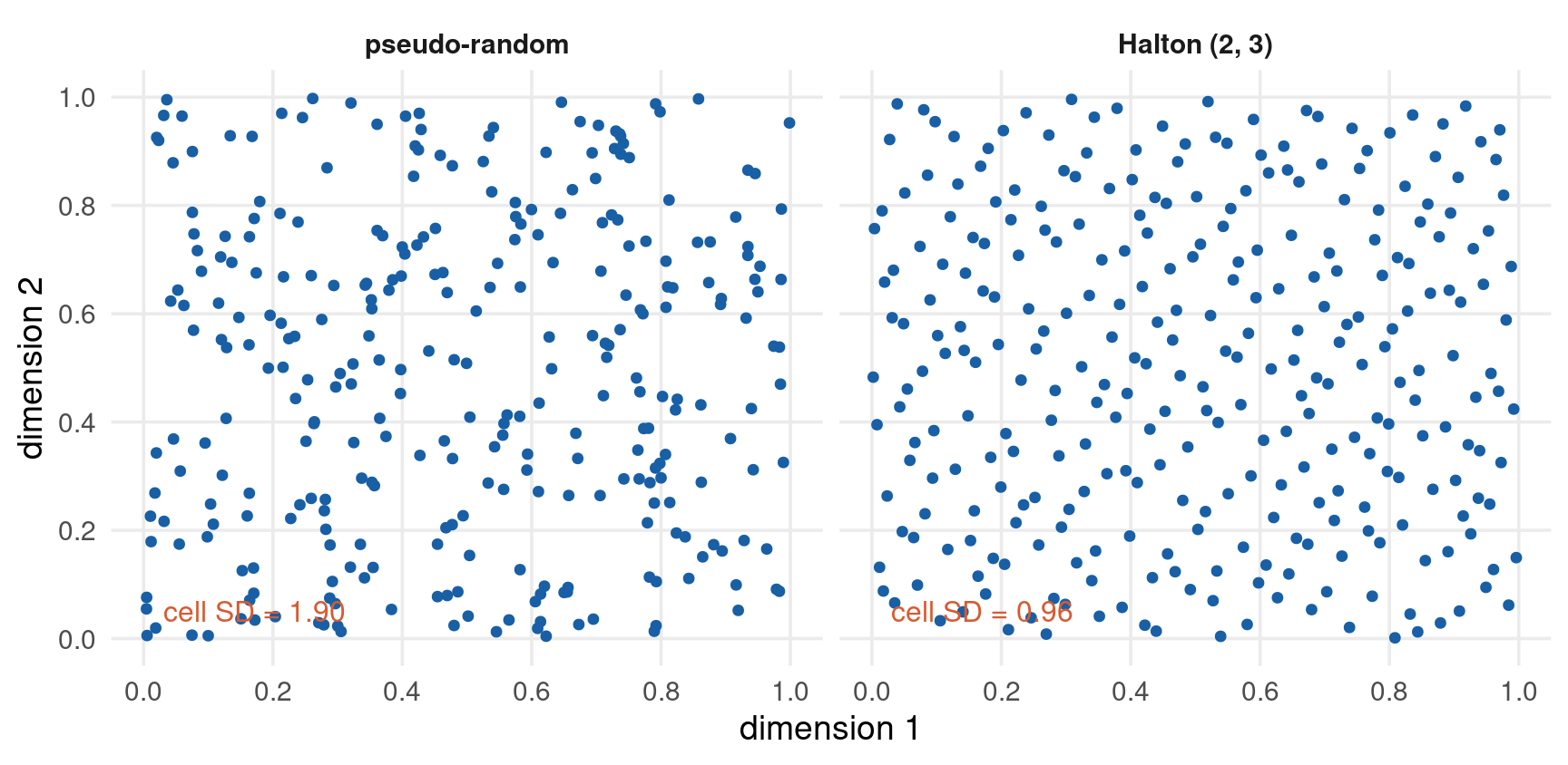
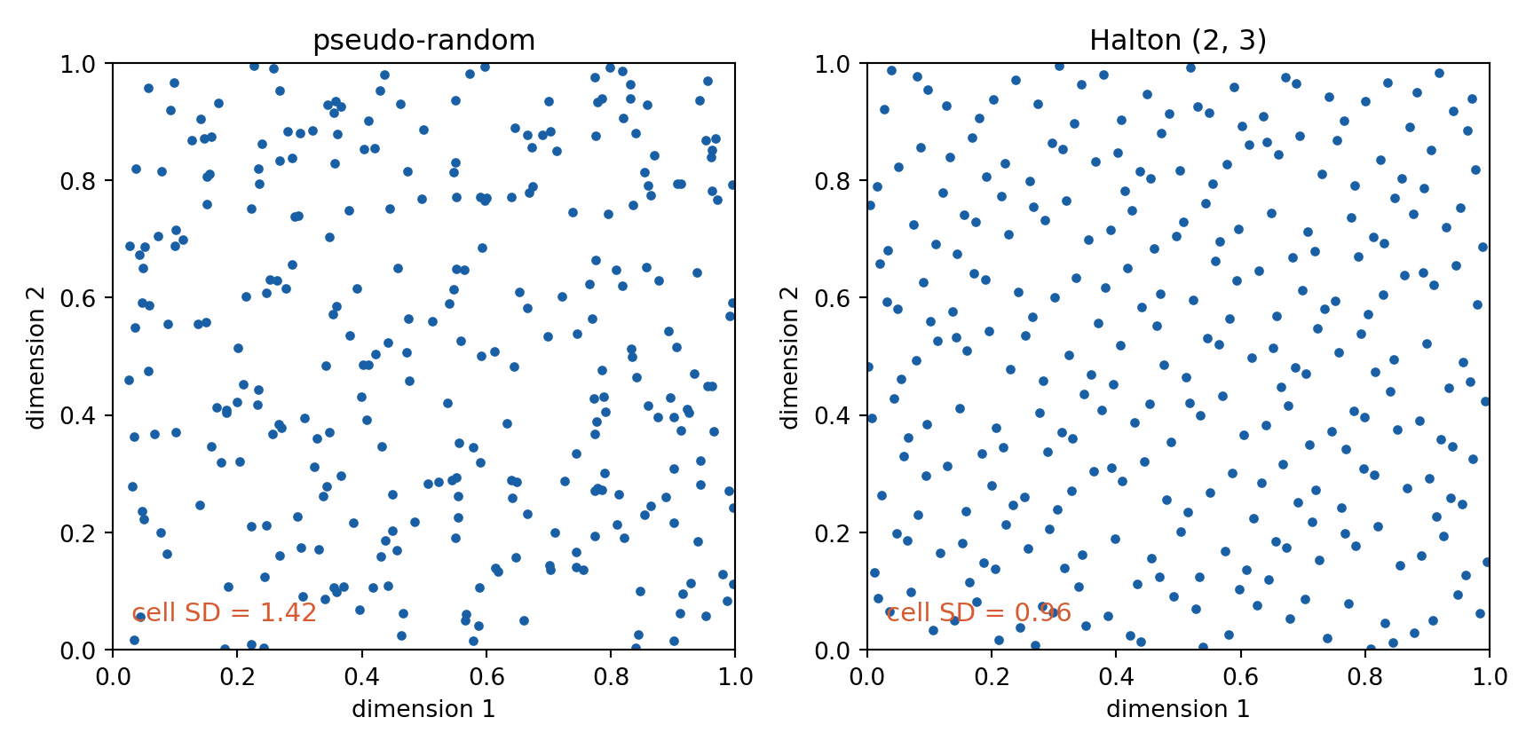
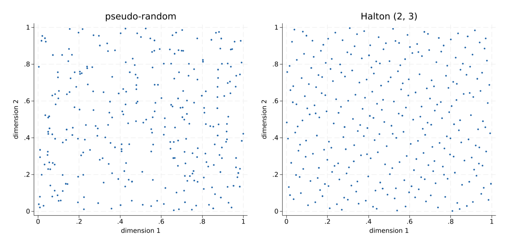
300 points in the unit square: pseudo-random against Halton. The number on each panel is the standard deviation of counts over a \(10 \times 10\) grid — perfect coverage would put exactly 3 points in every cell.
Code
# radical inverse: the whole of Halton in five lineshalton1 <-function(n, base, skip =10) { out <-numeric(n)for (i inseq_len(n)) { k <- i + skip f <-1 r <-0while (k >0) { f <- f / base r <- r + f * (k %% base) k <- k %/% base } out[i] <- r } out}set.seed(14159)R <-300pr <-data.frame(x =runif(R), y =runif(R), kind ="pseudo-random")hl <-data.frame(x =halton1(R, 2), y =halton1(R, 3), kind ="Halton (2, 3)")pts <-rbind(pr, hl)cellsd <-function(x, y) sd(table(cut(x, 0:10/10), cut(y, 0:10/10)))labs <-c(sprintf("cell SD = %.2f", cellsd(pr$x, pr$y)),sprintf("cell SD = %.2f", cellsd(hl$x, hl$y)))ggplot(pts) +aes(x = x, y = y) +geom_point(colour ="#185FA5", size =1.4) +facet_wrap(~ kind) +geom_text(data =data.frame(kind =unique(pts$kind), lab = labs),aes(x =0.03, y =0.05, label = lab),hjust =0, colour ="#D85A30", size =4.2, inherit.aes =FALSE) +coord_cartesian(xlim =c(0, 1), ylim =c(0, 1)) +scale_x_continuous(breaks =0:5/5) +scale_y_continuous(breaks =0:5/5) +labs(x ="dimension 1", y ="dimension 2") + theme_lecture
Code
import numpy as npimport matplotlib.pyplot as pltfrom scipy.stats import qmcrng = np.random.default_rng(14159)R =300pr = rng.random((R, 2))hl = qmc.Halton(d=2, scramble=False).random(R +10)[10:] # skip the first 10def cellsd(p): H, _, _ = np.histogram2d(p[:, 0], p[:, 1], bins=[np.arange(11)/10]*2)return H.std()fig, axes = plt.subplots(1, 2, figsize=(9, 4.4))for ax, p, ttl inzip(axes, [pr, hl], ["pseudo-random", "Halton (2, 3)"]): ax.scatter(p[:, 0], p[:, 1], s=9, color="#185FA5")# the number goes ON the figure: a Python chunk that draws also drops stdout ax.text(0.03, 0.05, "cell SD = %.2f"% cellsd(p), color="#D85A30", fontsize=11) axopts = ax.set(xlim=(0, 1), ylim=(0, 1), xticks=np.arange(6)/5, yticks=np.arange(6)/5, xlabel="dimension 1", ylabel="dimension 2", title=ttl)plt.tight_layout()plt.show()
Code
clearsetobs 300setseed 14159mata:// radical inverse of n in base b -- the whole of Haltonrealcolvector halton1(realscalar n, realscalar base, realscalar skip){realcolvector outrealscalar i, k, f, r out = J(n, 1, 0)for (i = 1; i <= n; i++) {k = i + skip; f = 1; r = 0while (k > 0) { f = f / baser = r + f * mod(k, base)k = floor(k / base) } out[i] = r }return(out)}st_addvar("double", ("hx", "hy"))st_store(., "hx", halton1(300, 2, 10))st_store(., "hy", halton1(300, 3, 10))endgendouble px = runiform()gendouble py = runiform()twoway (scatter py px, msize(vsmall) mcolor("24 95 165")), ///xscale(range(0 1)) yscale(range(0 1)) ///xlabel(0(0.2)1) ylabel(0(0.2)1) ///xtitle("dimension 1") ytitle("dimension 2") ///title("pseudo-random") legend(off) name(g1, replace) nodrawtwoway (scatter hy hx, msize(vsmall) mcolor("24 95 165")), ///xscale(range(0 1)) yscale(range(0 1)) ///xlabel(0(0.2)1) ylabel(0(0.2)1) ///xtitle("dimension 1") ytitle("dimension 2") ///title("Halton (2, 3)") legend(off) name(g2, replace) nodrawgraphcombine g1 g2, rows(1) xsize(9) ysize(4.4)graphexport"../plots/dchoice-halton.png", replacewidth(1600)
If \(u\) is redrawn at each evaluation, then two calls at the same\(\theta\) return different values. The objective is no longer a function, gradients are meaningless, and the optimiser terminates on noise. With \(u\) fixed, \(\hat\ell(\theta)\) is a deterministic, smooth surface — a slightly wrong one, but one that can be maximised.
This is the same device the companion deck Moments-Based Structural Estimation uses to smooth a simulated moment objective. There it removes chatter from a criterion function; here it makes a simulated likelihood differentiable. Seeing it twice, in two literatures, is the point — it is one idea, not two.
In a panel mixed logit the draws are per decision-maker, not per observation. Individual \(n\)’s taste \(\beta_n\) is fixed across their choice situations, so the same draws must be used for all of \(n\)’s choices — that is what distinguishes the panel likelihood from the cross-sectional one.
Using fresh draws per observation silently estimates a different model, in which tastes are redrawn every time someone makes a decision. It will run, converge, and be wrong.
Part 6 — Mixed Logit by MSL
Random coefficients, and what it costs to estimate them
Every model so far imposed one \(\beta\) on everybody. A commuter who cannot bear waiting and one who reads on the platform are given the same coefficient on out-of-vehicle time, and the difference between them is swept into \(\varepsilon\).
Mixed logit puts it in the model instead. Let each decision-maker have their own coefficient vector, drawn from a population distribution:
The analyst no longer estimates \(\beta\). The analyst estimates \(\theta\) — the parameters of the taste distribution, typically a mean vector and a covariance matrix.
Conditional on \(\beta_n\), the model is a logit and IIA holds. Unconditionally it does not, and the mechanism is worth stating precisely.
Two alternatives that load on the same attribute share the same random coefficient. Someone who happens to have a strong taste for that attribute finds both more attractive at once, so their unobserved utilities move together:
Correlation across alternatives arises from shared tastes rather than from an assumed tree or a free covariance matrix. Nothing has to be specified about which alternatives resemble which — that follows from the attributes.
Averaging the logit formula over the taste distribution returns the integral this deck opened with:
It has no closed form for any interesting \(f\). The dimension of the integral is the number of random coefficients, and it must be evaluated once per decision-maker per likelihood evaluation.
McFadden and Train (2000) proved something unusually strong. For any random utility model with choice probabilities \(P_{ni}\), and any \(\varepsilon > 0\), there exists a mixed logit with
for all \(i\) and \(n\) — given a suitable mixing distribution and enough flexibility in \(V\).
Mixed logit is not one more model in the catalogue. It is a universal approximator within the random-utility class.
Does mean: no substitution pattern is beyond reach in principle. If probit can represent it, so can mixed logit. There is no need for a menu of GEV forms.
Does not mean: that any particular mixed logit you estimate is flexible enough. The theorem is an existence result. In practice \(f\) is chosen from a short list — normal, lognormal, triangular — and that choice is a restriction every bit as real as a nesting tree.
Compare with Part 4. Probit gets full generality through a free \(\Sigma\) and pays with a \((J-1)\)-dimensional integral. Mixed logit gets it through the taste distribution and pays with an integral whose dimension is the number of random coefficients — which is often far smaller. That is why mixed logit, not probit, became the workhorse.
A normal coefficient on price puts positive mass on \(\beta_{\text{price}} > 0\): some share of the population is modelled as preferring to pay more. With a mean far from zero relative to the standard deviation this is a small nuisance; when the estimated \(\sigma\) is large it is a serious misspecification, and the implied willingness-to-pay distribution has mass at the wrong sign.
The lognormal fixes the sign by construction, since \(e^{z} > 0\) always. But a lognormal variate is positive, and a price coefficient must be negative — so the variable has to enter negated:
which in code means creating negcost = -cost and putting the lognormal on that.
This is not a stylistic point. Ask mlogit for a lognormal coefficient on a variable whose coefficient is negative and it fails outright with NaNs produced in log(start) — it cannot even build starting values. The DGP of dchoice-mixed.csv was written with the sign flip in it deliberately, so every tab below has to handle it.
Packages report \(\mu\) and \(\sigma\) of the underlying normal, not of the coefficient. Convert before interpreting:
For this deck’s truth, \(\mu = -0.3\) and \(\sigma = 0.5\), so the median cost sensitivity is \(e^{-0.3} = 0.741\) and the mean is \(e^{-0.175} = 0.839\). A reported coefficient of \(-0.35\) is not the taste — it is the log-scale location parameter.
The draws are generated from standard uniforms/normals fixed in advance and transformed by \(\theta\) at each iteration — common random numbers again, exactly as in Part 5.
With repeated choices, the taste is drawn once per person, and their whole sequence of choices is conditioned on that same \(\beta_n\):
The product inside the average is what identifies the taste distribution. Move it outside and the model collapses to one where tastes are redrawn at every occasion — which is a different, and much weaker, model.
This is why dchoice-mixed.csv is a panel of 500 people × 8 situations rather than 4000 independent choices. Estimated cross-sectionally, the same design returns \(\hat\sigma_{\text{qual}} = 0.86\) against a truth of \(0.70\); as a panel it returns \(0.71\). Repeated choices are what make the taste distribution visible.
\(\hat P\) is unbiased for \(P\), but the criterion uses \(\log \hat P\), and Jensen gives \(\mathbb{E}[\log \hat P] < \log P\). So the simulated log-likelihood is biased downward for every finite \(R\), and MSL is:
inconsistent for fixed \(R\) as \(N \to \infty\)
consistent if \(R \to \infty\) with \(N\)
asymptotically equivalent to true ML only if \(\sqrt{N}/R \to 0\)
That last condition is the next slide, and it is the one people ignore.
\[\frac{\sqrt{N}}{R} \longrightarrow 0
\qquad\Longleftrightarrow\qquad
R \text{ must grow faster than } \sqrt{N}\]
The simulation bias in the log-likelihood is \(O(R^{-1})\). Spread over \(N\) observations, the induced bias in \(\hat\theta\) is of order \(N/R\) relative to the \(\sqrt{N}\) sampling noise. Only if \(R\) outgrows \(\sqrt{N}\) does the simulation bias vanish faster than the standard error, leaving the asymptotic distribution undisturbed.
\(N\)
\(\sqrt{N}\)
\(R\) must exceed
1 000
32
a few hundred
10 000
100
around a thousand
100 000
316
several thousand
Why the condition is \(\sqrt{N}/R\) and not \(N/R\)
Two quantities are racing, and the condition is about which wins.
Sampling noise. Ordinary maximum likelihood gives \(\hat\theta - \theta_0 = O_p(N^{-1/2})\). Scaled up for inference, \(\sqrt{N}(\hat\theta - \theta_0)\) converges to a normal distribution with a finite variance.
Simulation bias. Part 4’s expansion showed each observation’s \(\log \hat{P}\) carries a bias of order \(R^{-1}\). It is the same sign for every observation, so averaging over \(N\) does not shrink it — the induced bias in \(\hat\theta\) stays \(O(R^{-1})\).
Now apply the \(\sqrt{N}\) scaling that inference requires, and the bias term becomes
For the limiting distribution to stay centred at zero, that must vanish — hence \(\sqrt{N}/R \to 0\).
The \(\sqrt{N}\) appears because it is the scaling used for inference, not because the bias itself grows with \(N\). Confidence intervals shrink like \(N^{-1/2}\) while the bias does not shrink at all, so eventually the bias is large relative to the interval.
Fail the condition and the estimator is still consistent if \(R \to \infty\); what breaks is the asymptotic distribution. Point estimates look fine, coverage does not.
The sampling noise is \(O_p\) and averages out; the simulation bias is deterministic in sign and does not. That asymmetry is the whole argument.
The condition is asymptotic and says nothing about how large \(R\) must be on your data. Two honest consequences:
more data demands more draws. Doubling the sample and keeping \(R\) fixed makes the simulation bias relatively worse, not better
a large-\(N\) study with \(R = 50\) is not “approximately” maximum likelihood; it is a different, biased estimator
Quasi-random sequences change the constant, not the requirement. Halton draws reduce the error at any given \(R\) by an order of magnitude — Part 5’s table — which is why 200 Halton draws are often adequate where thousands of pseudo-random draws would be needed.
The practical test is the one Part 5 recommended and the noise slide below performs: re-estimate at \(2R\) and \(4R\). If the estimates and their standard errors are stable, \(R\) is large enough for this sample. If they drift, it is not.
Code — Mixed Logit on Known-Truth Data
500 individuals × 8 choice situations × 4 alternatives. Truth: ASCs \((0.4, -0.3, 0.2)\); qual normal with mean \(1.0\) and sd \(0.7\); cost entering as a lognormal on \(-\text{cost}\) with \(\mu = -0.3\), \(\sigma = 0.5\). 200 Halton draws throughout.
Code
library(mlogit)library(dplyr)set.seed(14159)mx <-read.csv("../data/dchoice-mixed.csv") |>mutate(negcost =-cost) # lognormal needs a positive coefficient# panel index: choice situation nested in individual, then alternativeMX <-dfidx(mx, idx =list(c("chid", "id"), "altnum"), choice ="choice")mxl <-mlogit(choice ~ qual + negcost |1, data = MX,rpar =c(qual ="n", negcost ="ln"),R =200, halton =NA, panel =TRUE)summary(mxl)
import warnings; warnings.filterwarnings("ignore")import numpy as np, pandas as pdfrom xlogit import MixedLogitdf = pd.read_csv("../data/dchoice-mixed.csv")df["negcost"] =-df["cost"]# xlogit's lognormal does NOT converge from its default start; any sane# starting vector reaches the same optimum. This one is NOT the truth.start = np.array([0.0, 0.0, 0.0, 0.5, -0.5, 0.3, 0.3])m = MixedLogit()m.fit(X=df[["qual", "negcost"]], y=df["choice"], varnames=["qual", "negcost"], alts=df["altnum"], ids=df["chid"], panels=df["id"], randvars={"qual": "n", "negcost": "ln"}, n_draws=200, halton=True, fit_intercept=True, base_alt=1, random_state=14159, init_coeff=start)m.summary()
The estimator finds the taste distribution. The standard deviations — the parameters that exist only because tastes are heterogeneous — come back at 0.7145 against 0.70 and 0.5077 against 0.50. Those are the hard parameters, and they are recovered.
R and Python agree to every printed digit. Both use Halton draws with the same construction, so with the same seed they evaluate the same simulated likelihood and find the same optimum. This is stronger agreement than is usual across packages.
Stata differs in the third decimal, for a reason.cmxtmixlogit integrates with a Hammersley sequence, not Halton. Different draws, different simulated objective, slightly different optimum — a \(0.099\) gap in the log-likelihood.
That last row is the lesson of Parts 5 and 6 in one line. The draws are part of the estimator. Two correct implementations of the same model disagree in the third decimal purely because they integrate with different sequences, and neither is wrong. Report the sequence and the number of draws, or your result is not reproducible.
Simulation Noise
How much of the answer is the data, and how much is the draws? The same model, the same seed, only \(R\) changing.
for (Rd inc(50, 100, 200, 500, 1000)) {set.seed(14159) f <-mlogit(choice ~ qual + negcost |1, data = MX,rpar =c(qual ="n", negcost ="ln"),R = Rd, halton =NA, panel =TRUE) b <-coef(f)cat(sprintf("R =%5d LL =%12.4f qual =%7.4f sd.qual =%7.4f sd.negcost =%7.4f\n", Rd, as.numeric(logLik(f)), b["qual"], b["sd.qual"], b["sd.negcost"]))}
R =   50   LL =  -4191.9824   qual = 0.9500   sd.qual = 0.7225   sd.negcost = 0.5133
R =  100   LL =  -4191.4983   qual = 0.9437   sd.qual = 0.7119   sd.negcost = 0.5169
R =  200   LL =  -4190.4744   qual = 0.9442   sd.qual = 0.7145   sd.negcost = 0.5077
R =  500   LL =  -4190.6496   qual = 0.9463   sd.qual = 0.7110   sd.negcost = 0.5198
R = 1000   LL =  -4190.3275   qual = 0.9473   sd.qual = 0.7113   sd.negcost = 0.5186
truth: qual = 1.0000 sd.qual = 0.7000 sd.negcost = 0.5000
Two things to look for, and they are different questions.
Is the answer stable? Compare the coefficient columns as \(R\) doubles. Drift that exceeds a fraction of a standard error means \(R\) is too small. Here the estimates settle quickly — the Halton draws are doing their job.
Is the likelihood comparable? The simulated log-likelihood is not comparable across different \(R\). It is an average of \(R\) terms and its bias is \(O(R^{-1})\), so a model with more draws will tend to report a higher simulated log-likelihood for that reason alone.
Never compare information criteria across models estimated with different numbers of draws. An AIC comparison between a model at \(R = 100\) and one at \(R = 1000\) measures the draw count, not the fit. Fix \(R\) across every specification in a table, and say what it was.
Nothing forces the elements of \(\beta_n\) to be independent. The general specification is
\[\beta_n = b + L \eta_n, \qquad \eta_n \sim N(0, I),
\qquad \text{Var}(\beta_n) = LL'\]
with \(L\) lower triangular and estimated. Someone who cares a lot about time may also care a lot about cost, and the off-diagonal elements of \(LL'\) capture that.
The cost is parameters: \(K\) random coefficients need \(K(K+1)/2\) elements of \(L\), so the count grows quadratically and the integral’s dimension grows with \(K\). Most applied work estimates a diagonal \(L\) and says so.
The specification above is in preference space: the coefficients are random, and WTP is a ratio of two random variables. Its distribution is therefore a ratio distribution — often heavy-tailed, sometimes with no finite mean, which is a genuine problem when WTP is the reported quantity.
WTP space reparameterises so the object of interest is the primitive:
Here \(\omega_n\)is the willingness-to-pay vector and \(\lambda_n\) is the scale. Distributional assumptions are made directly on WTP, so its distribution is whatever was assumed rather than an uncontrolled ratio.
The trade-off is real and unresolved: preference space usually fits better, WTP space gives better-behaved welfare numbers. Train and Weeks (2005) is the reference.
Mixed logit estimates a population distribution, but the observed choices carry information about where in that distribution each person sits. Bayes’ rule on the individual’s own choice sequence:
which is computed from the same draws already in hand — a weighted average of the \(\beta^{(r)}\), with weights proportional to how well each explains that person’s choices.
Code
# conditional means of beta_n, from the fitted mixed logitpost <-fitted(mxl, type ="parameters")cat("individual-level conditional means of the qual coefficient\n")
individual-level conditional means of the qual coefficient
Code
print(summary(post[, "qual"]))
   Min. 1st Qu.  Median    Mean 3rd Qu.    Max.
-0.5718  0.5704  0.9732  0.9472  1.3057  2.1234
These are not individual parameter estimates — with 8 choices per person they are shrunk heavily toward the population mean. They are useful for segmentation and targeting, and misleading if read as person-specific truths.
Part 7 — Intercity Travel Mode Choice
Three models, one dataset, and what actually changes
Travellers choosing between Montreal and Toronto, from the Canadian VIA Rail study analysed by Bhat (1995) and Koppelman & Wen (2000). The deck uses the standard noalt == 4 subsample: the 2779 travellers for whom all four modes were genuinely available, a complete \(2779 \times 4\) rectangle.
variable
meaning
cost
generalised cost, 1986 CAD
ivt
in-vehicle time, minutes
ovt
out-of-vehicle time — waiting, access, transfers
freq
departures per day
income
household income, thousands CAD (person-specific)
The policy question is the one transport agencies actually ask: what is an hour of a traveller’s time worth, and does the answer survive a change of model?
Bus is chosen by 10 travellers out of 2779 — a share of 0.36%. That is real, and it has consequences: the bus constant and income slope are estimated off ten observations, so their standard errors are large and any nest containing bus is fragile. A model can be correct and still contain a parameter that carries almost no information.
Estimate three models on identical data and compare them on the things that matter — not on coefficients, which Part 1 established are not comparable:
MNL — the Part 2 benchmark, with IIA imposed
nested logit — air against the ground modes, \(\lambda\) estimated
mixed logit — a random coefficient on in-vehicle time
Then read off fit, substitution patterns, and the value of travel time savings.
Part 2 promised that logit always converges, and warned that the promise expires at Part 6. Here is the expiry, on real data.
Estimating the mixed logit above from default starting values — zeros, which every logit routine uses safely — gives:
naive start
start at the MNL
simulated log-likelihood
−2598.07
−1897.05
ASC air
−255.95
1.86
ivt
−0.856
−0.0138
implied VTTS
110 CAD/hour
12.36 CAD/hour
The naive fit is 668 log-likelihood points worse than the MNL it nests, which is impossible at a true maximum. The optimiser reported convergence, every \(z\)-statistic was enormous, and every number was wrong.
Nothing in the output announces the failure. What catches it is arithmetic the analyst has to do:
compare against the nested simpler model. A mixed logit must beat its own MNL; if it does not, it has not converged
sanity-check the implied economics. 110 CAD/hour in 1986 dollars is not a plausible value of time
restart from the simple model’s estimates. Standard practice, not a trick: fit the MNL, use its coefficients as the starting vector, and give the standard deviations small positive starts
re-estimate from several starting points and confirm they agree
“It converged” is not evidence. For a globally concave objective, convergence proves a global maximum; for a simulated likelihood it proves only that the gradient got small somewhere. Every mixed logit in this deck is started from its MNL for exactly this reason.
The mixed-logit column reports R. The other two tabs give −1897.15 (Stata) and −1897.32 (Python) for the same specification — a spread of 0.27 in the simulated log-likelihood, from nothing but different draw sequences. The MNL and nested columns, which have no simulation in them, agree across all three languages to six decimals. That contrast is Part 6’s lesson appearing in a results table: simulation noise is the only thing separating these three numbers, and it is larger than the last two digits anyone would quote.
Code
res <-data.frame(model =c("MNL", "Nested", "Mixed"),logLik =c(as.numeric(logLik(mnl7)), as.numeric(logLik(nl7)),as.numeric(logLik(mxl7))),k =c(length(coef(mnl7)), length(coef(nl7)), length(coef(mxl7))),AIC =c(AIC(mnl7), AIC(nl7), AIC(mxl7)),BIC =c(AIC(mnl7, k =log(2779)), AIC(nl7, k =log(2779)),AIC(mxl7, k =log(2779))))print(transform(res, logLik =round(logLik, 4), AIC =round(AIC, 3),BIC =round(BIC, 3)), row.names =FALSE)
  model    logLik  k      AIC      BIC
    MNL -1930.565 10 3881.130 3940.429
 Nested -1927.326 11 3876.652 3941.880
  Mixed -1897.050 11 3816.100 3881.328
Akaike's information criterion and Bayesian information criterion

-----------------------------------------------------------------------------
       Model |          N   ll(null)  ll(model)      df        AIC        BIC
-------------+---------------------------------------------------------------
          M1 |      2,779          .  -1930.565      10    3881.13   3940.429
          M2 |      2,779          .  -1897.149      11   3816.297   3881.525
-----------------------------------------------------------------------------
Note: BIC uses N = number of cases. See [R] IC note.
Both models add exactly one parameter to the MNL, so the comparison is unusually clean: the same degree of freedom buys ten times more log-likelihood when spent on a random coefficient than on a nest.
BIC agrees, which matters because BIC penalises harder. The mixed logit wins on BIC (3881.3 against 3940.4 and 3941.9), while the nested logit’s BIC is actually worse than the MNL’s — its one extra parameter does not pay for itself under the stricter penalty.
Mixed logit and nested logit are not nested in each other, so no likelihood-ratio test applies. The options:
AIC / BIC — appropriate, and both favour the mixed logit here
Vuong’s test — a formal non-nested test, though its behaviour with simulated likelihoods is not well established
out-of-sample fit — hold out travellers and compare predicted log-likelihood; the most persuasive option and the least often used
Every comparison here fixes \(R = 200\) across specifications. The simulated log-likelihood depends on the draw count, so a table mixing \(R = 100\) and \(R = 1000\) compares draws, not models. This is the trap Part 6 flagged, and it is easy to walk into when models are estimated at different times.
Substitution Patterns
Aggregate elasticity of every mode’s predicted share with respect to a 1% rise in the cost of air travel, computed by re-predicting on perturbed data.
               car  train     air    bus
MNL         1.1455 1.6224 -2.1312 1.1845
Mixed logit 0.9912 1.4964 -1.9424 1.0146
The three non-air entries are not equal in either row, and it would be wrong to read that as the MNL violating IIA. Two different things are going on.
IIA is an individual-level property. Part 2 showed the MNL’s cross-elasticities being exactly equal — at a single representative decision-maker. That equality is algebraic and exact.
Aggregation breaks it even under IIA. These travellers differ in observed income, so they have different choice probabilities, and a share-weighted average of individually-proportional responses is not itself proportional. Observed heterogeneity alone produces unequal aggregate elasticities.
What the mixed logit adds is unobserved heterogeneity on top of that. Its elasticities are uniformly smaller in magnitude — air’s own-elasticity moves from about \(-2.13\) to \(-1.94\) — because travellers with a strong distaste for in-vehicle time are less responsive to air fares at the margin. Whether that difference matters is a policy question, and it is exactly the question the extra parameter was bought to answer.
vtts <-function(fit, v ="ivt") { b <-coef(fit); V <-vcov(fit) r <- b[v] / b["cost"] g <-c(1/ b["cost"], -b[v] / b["cost"]^2) se <-sqrt(t(g) %*% V[c(v, "cost"), c(v, "cost")] %*% g)c(est =60* r, lo =60* (r -1.96* se), hi =60* (r +1.96* se))}tab <-rbind(MNL =vtts(mnl7), Nested =vtts(nl7), Mixed =vtts(mxl7))cat("Value of in-vehicle travel time savings, CAD per hour (1986)\n\n")
Value of in-vehicle travel time savings, CAD per hour (1986)
Code
print(round(tab, 4))
       est.ivt     lo      hi
MNL    13.3256 9.8182 16.8330
Nested 13.4454 9.8325 17.0583
Mixed  12.3599 8.7971 15.9228
The three models disagree about almost every coefficient, about the substitution pattern, and about the fit. They agree about the number that goes into the appraisal:
That is Part 1’s identification argument arriving with real numbers. Coefficients are scale-dependent and not comparable across models; ratios of coefficients are scale-free, and the ratio is stable across three specifications whose log-likelihoods span 33 points.
The delta method, worked through
With \(r = \beta_{\text{ivt}}/\beta_{\text{cost}}\), take a first-order expansion around the true values. The gradient is
For the MNL: \(\hat\beta_{\text{ivt}} = -0.009986\), \(\hat\beta_{\text{cost}} = -0.044963\), giving \(r = 0.2221\) CAD per minute, \(\times 60 = 13.33\) CAD per hour, with a standard error of \(1.79\).
Where this approximation fails. Note the \(\beta_c^{4}\) in the last term. As the cost coefficient approaches zero relative to its own standard error, the variance explodes and the linearisation stops describing the true sampling distribution:
The exact distribution of a ratio of two normals is Cauchy-like when the denominator has mass near zero — heavy-tailed, and with no finite mean.
The symmetric interval \(\hat r \pm 1.96\,\mathrm{se}\) then understates the uncertainty badly, and can even be the wrong shape entirely.
A useful rule of thumb: trust it while \(|t|\) on the denominator exceeds about 5. Here \(t_{\text{cost}} = -11.4\), comfortably safe.
Fixes. Fieller’s method inverts a \(t\)-test on \(\beta_{\text{ivt}} - r\beta_{\text{cost}} = 0\) and gives correct — sometimes unbounded — intervals. The bootstrap makes no normality assumption at all; see the companion deck Bootstrap Methods in Econometrics. WTP-space estimation, from Part 6, avoids the ratio altogether by making WTP a primitive parameter.
The confidence intervals are wide — roughly \(\pm 30\%\) — and they overlap almost completely across models. Model choice is not the binding constraint on this policy number; sample size is. An analyst arguing about nesting structure while reporting a CI of \([9, 17]\) is optimising the wrong thing.
The MNL put out-of-vehicle time at roughly four times the value of in-vehicle time per minute — 57 CAD/hour against 13. Waiting on a platform costs travellers far more than sitting on a train, and that ratio is one of the most reliably reproduced findings in transport economics.
It has a direct policy reading: a timetable change that removes waiting is worth several times a speed increase saving the same number of minutes in transit. None of this is visible in the raw coefficients, which is the argument for reporting ratios in the first place.
Part 6 made the point with numbers: the same design estimated cross-sectionally returns \(\hat\sigma_{\text{qual}} = 0.86\) against a truth of \(0.70\), and as a panel returns \(0.71\). Repeated choices are what make a taste distribution visible rather than merely assumed.
The likelihood conditions each person’s whole sequence on one draw of their taste:
The product sits inside the average. That ordering is the entire difference between a panel mixed logit and a cross-sectional one, and getting it backwards gives a model that runs, converges, and answers a different question.
# R -- three-level index: situation nested in individual, then alternativeMX <-dfidx(mx, idx =list(c("chid", "id"), "altnum"), choice ="choice")mlogit(choice ~ qual + negcost |1, MX, rpar =c(qual ="n"),R =200, halton =NA, panel =TRUE)
# Python -- panels= is what distinguishes it from ids=MixedLogit().fit(..., ids=df["chid"], panels=df["id"], ...)
* Stata -- cmset with THREE variables declares the panelcmset id chid altnumcmxtmixlogit choice, random(qual) intpoints(200)
The commonest error in applied work is passing the choice-situation identifier where the person identifier belongs. Nothing fails — the model estimates a world in which tastes are redrawn afresh at every decision, and the standard deviations come back too small. Check that the number of panels equals the number of people, not the number of choices.
State dependence — include the previous choice in \(V\); be careful to separate genuine habit from persistent unobserved taste, which is Heckman’s initial-conditions problem
Stated-preference experiments — the canonical panel: each respondent answers 8–16 designed choice tasks, and the experimental design controls attribute variation directly
Scale heterogeneity — respondents differ in how consistently they choose, not only in what they prefer; the G-MNL of Fiebig et al. (2010) separates the two
Mixed logit assumes tastes are spread continuously through the population. Latent class logit assumes there are \(C\)types, each with its own coefficient vector, and that nobody knows who belongs to which:
The integral becomes a finite sum, so there is nothing to simulate. Class shares \(\pi_c\) can themselves depend on covariates through a logit, which is often where the interesting economics sits.
mixed logit
latent class
heterogeneity
continuous
\(C\) discrete types
computation
simulation, \(R\) draws
closed-form sum
choosing dimension
choose \(f\)
choose \(C\)
output
a distribution
interpretable segments
risk
wrong parametric \(f\)
wrong \(C\); local optima
Neither dominates. Latent class is attractive when the story is genuinely about segments — business versus leisure travellers — and its output is easier to present to non-technical audiences. Mixed logit is more natural when taste varies smoothly.
Both have the same trap in different clothing: \(C\) and \(f\) are chosen by the analyst and are not tested by the data in any strong sense. The likelihood ratio test for \(C\) versus \(C+1\) classes does not have a \(\chi^2\) distribution — the parameters of the extra class are unidentified under the null. Use BIC and substantive interpretability, and say what you did.
Why the LR test for \(C\) classes is invalid
Test \(C = 1\) against \(C = 2\). The two-class model is
and the null “one class” can be reached in two different ways, which is the whole problem:
set \(\pi = 0\) — then \(\beta_1\) is unidentified, because it multiplies a class of zero size and the likelihood does not depend on it at all;
set \(\beta_1 = \beta_2\) — then \(\pi\) is unidentified, because both classes are the same and any mixing weight gives an identical likelihood.
Either way a nuisance parameter is present only under the alternative. Two standard regularity conditions fail at once:
the null sits on the boundary of the parameter space, since \(\pi \ge 0\);
the information matrix is singular at the null, so the usual quadratic expansion of the log-likelihood does not exist.
The consequence is that \(2(\ell_2 - \ell_1)\) is not\(\chi^2_k\) for any \(k\). Its true limiting distribution is the supremum of a Gaussian process indexed by the unidentified parameter, and in practice the naive test over-rejects — it finds classes that are not there.
What to do instead:
BIC, which is the field’s default for choosing \(C\) and penalises extra classes heavily;
a parametric bootstrap of the LR statistic, simulating under the \(C\)-class null to get the correct critical value — expensive but principled;
substantive interpretability: a class that cannot be described in words is usually an artefact of a local optimum, and latent class models have many of those. Estimate from multiple starts.
The identical issue arises when testing whether a mixed-logit standard deviation is zero: \(\sigma \ge 0\) puts the null on the boundary, so that statistic is not \(\chi^2_1\) either. Exercise 6 in the estimation set asks about exactly this.
Implementations: R gmnl or flexmix; Stata lclogit2 (SSC); Python has no maintained implementation, so the sum has to be hand-coded — which, given the closed form, is genuinely easy.
Everything so far needed individual choice data: who chose what, and what the alternatives looked like. Very often that does not exist. What exists is market shares — how much of each product sold, in each market, at what price.
Two new problems arrive at once:
the data are aggregate, so the individual likelihood cannot be written
price is endogenous, because firms set it knowing the unobserved product quality \(\xi_j\) that also drives demand
Ordinary logit on aggregate shares gets price elasticities badly wrong, and — as Part 3 showed — imposes proportional substitution between every pair of products, which is hopeless for differentiated goods.
Berry, Levinsohn and Pakes (1995) solve both problems using the machinery of this deck as a component:
random coefficients on price and product characteristics generate realistic substitution — a price rise for one car sends buyers to similar cars. This is Part 6, unchanged
the contraction mapping inverts observed market shares to recover the mean utility \(\delta_j\) that rationalises them, for any candidate parameter vector
instruments then handle price endogeneity in the resulting linear equation via GMM
The inner loop simulates market shares by exactly the method of Part 6, with the same draws held fixed for the same reason, and Halton or Sobol sequences for the same efficiency gain.
The companion deck Structural Estimation in Econometrics owns BLP and Rust’s dynamic discrete choice. It uses random coefficients and simulated shares as given. This deck is where they come from: what the mixing distribution is, why the integral has no closed form, how it is simulated, and what the draws cost. Read them in that order.
Dynamic discrete choice — Rust (1987): the alternatives are actions today with consequences tomorrow, and \(V\) becomes a value function solved by fixed point
Semi- and non-parametric — Klein–Spady, and Matzkin’s identification results, which drop the distributional assumption on \(\varepsilon\) altogether
Bayesian mixed logit — hierarchical Bayes with Gibbs/Metropolis avoids MSL’s bias entirely and gives individual-level posteriors directly; see Bayesian Computation in Economics and Econometrics
Machine learning for choice — a classifier predicts the choice well but recovers no preferences, so no welfare, no WTP, no counterfactual. Different tool, different question
Comparing coefficients across models. Scale differs by construction. Compare ratios, elasticities and predicted probabilities.
A lognormal on a variable whose coefficient is negative. Negate the variable first; mlogit will not even build starting values otherwise.
Reading lognormal \(\mu\) as the taste. It is the location of the underlying normal. The median is \(e^{\mu}\).
Person-specific regressors entered generically. Income has no alternative-specific coefficient? Then it has dropped out of every utility difference and does nothing.
A nest whose \(\hat\lambda > 1\). Inadmissible, no matter how well it fits.
Too few draws, never checked. Re-estimate at \(2R\) and \(4R\). If nothing moves, report \(R\); if things move, raise it.
Redrawing at each iteration. The objective stops being a function; use common random numbers.
Comparing information criteria across different \(R\). The simulated log-likelihood is biased by \(O(R^{-1})\); a table mixing draw counts compares draws.
Fresh draws per observation in a panel. Silently estimates a different model with far too little heterogeneity.
Raw Halton beyond ten dimensions. Use scrambled Halton or Sobol.
Trusting “converged”. Only concave objectives make that informative — Part 7’s failure was 668 log-likelihood points from the truth and reported success.
Over-reading an IIA test. This deck’s Hausman–McFadden statistics were negative, in all three languages. A non-rejection is very weak evidence.
Choosing a nesting tree by fit. The admissible set comes first.
Treating individual-level posteriors as person-specific estimates. They are shrunk heavily toward the population mean.
Reporting a delta-method WTP interval when the denominator is imprecise. Use the bootstrap or Fieller.
Forgetting the base alternative differs across packages. Pin it explicitly in all three.
the choice set — alternatives, and how availability was determined
sample size in both units: decision-makers and observations
choice shares, so degenerate alternatives like this deck’s bus are visible
the base alternative and the scale normalisation
for random coefficients: which coefficients, and with what distribution
the number of draws and the sequence — “200 scrambled Halton”, not “simulated”
starting values for any simulated likelihood, and evidence of a stable optimum
elasticities or marginal effects, not just coefficients
WTP with an interval, and how the interval was constructed
the specifications you tried and rejected, not only the survivor
situation
model
few alternatives, IIA plausible, need speed
MNL
alternatives fall into clear groups you can defend
nested logit
need one free correlation structure, few alternatives
MNP
tastes plausibly vary; want any substitution pattern
mixed logit
heterogeneity is about interpretable segments
latent class
repeated choices per person
panel mixed logit
only market-level shares, endogenous prices
BLP — see the structural deck
choice set in the thousands
MNL with sampling of alternatives
prediction only, no welfare or counterfactual
a classifier — but then say so
Start at the top of the table and move down only when something forces you. Part 7’s mixed logit beat the MNL decisively on fit and moved the headline policy number by less than one standard error. Extra structure has to earn its place, and “it fits better” is not automatically the same as “it changes the answer”.
Exercises — Estimation
Re-estimate the Part 2 MNL on ModeCanada dropping freq. Report how the value of travel time savings changes, and explain why omitting a variable that varies across alternatives moves a ratio of two other coefficients.
Fit the MNL with bus excluded from the choice set. Compare the coefficients with the full-choice-set fit. Given that bus is chosen 10 times out of 2779, is the difference what you expected?
Estimate the three nesting trees in the Part 3 comparison table yourself, and add a fourth of your own choosing. Report \(\hat\lambda\), its standard error, and the log-likelihood for each, and state which trees you would be willing to defend.
Using dchoice-mixed.csv, estimate the mixed logit with both coefficients normal instead of normal-and-lognormal. Compare the fit and the implied distribution of the cost coefficient with the known truth. What fraction of the population is assigned the wrong sign?
Re-estimate the Part 7 mixed logit from at least five different starting vectors, including the naive all-zeros start. Report the log-likelihood reached from each, and describe how you would detect a failed run without knowing the answer in advance.
Add a second random coefficient to the Part 7 mixed logit — ovt, say — and test whether its standard deviation differs from zero. Note that the null sits on the boundary of the parameter space, and say what that does to the distribution of the test statistic.
Estimate a latent class logit with \(C = 2\) and \(C = 3\) on ModeCanada, using gmnl in R or lclogit2 in Stata. Compare BIC with the Part 7 mixed logit and interpret the classes substantively.
Exercises — Testing and Simulation
Reproduce the Part 4 GHK convergence table, replacing pseudo-random draws with Halton. Confirm the gain reported in Part 5, then repeat in ten dimensions instead of three and report what happens to the advantage.
Implement the naive frequency simulator for the same orthant probability: draw from \(N(0,\Omega)\) and count. At \(R = 100\), report how often it returns exactly zero, and explain precisely why that breaks maximum simulated likelihood.
Verify the \(O(R^{-1/2})\) rate directly. For \(R \in \{50, \dots, 3200\}\), regress \(\log(\text{RMSE})\) on \(\log R\) and report the slope with a standard error. Do the same for Halton and compare the two slopes.
Take the Part 6 mixed logit and deliberately redraw the random numbers at every likelihood evaluation. Report what happens to the optimiser, and to the estimates if it terminates at all.
Run the Hausman–McFadden test dropping each alternative in turn. Report all four statistics and their signs, then argue whether any of them constitutes evidence about IIA on this dataset.
Implement the Small–Hsiao test and run it 200 times with different random splits. Plot the distribution of the statistic and of the resulting \(p\)-value, and state what that implies for a paper reporting a single Small–Hsiao result.
Using dchoice-probit.csv, estimate the restricted MNP of Part 4 at \(R \in \{25, 50, 100, 200, 400\}\) draws. Plot \(\hat\rho\) against \(R\) and identify where the simulation bias becomes smaller than the standard error.
Simulate your own choice data with a known non-nested substitution pattern, then estimate an MNL, a nested logit and a mixed logit on it. Report which model recovers the true cross-elasticities, and by how much the others miss.
Train (2009), Discrete Choice Methods with Simulation, 2nd ed., CUP — doi:10.1017/CBO9780511805271. The standard reference and the one to buy; this deck follows its notation and its ordering of topics.
Ben-Akiva & Lerman (1985), Discrete Choice Analysis, MIT Press — still unmatched on specification, normalisation and the practicalities of travel demand.
Hensher, Rose & Greene (2015), Applied Choice Analysis, 2nd ed., CUP — doi:10.1017/CBO9781316136232. The applied companion, strong on stated-preference design.
Cameron & Trivedi (2005), Microeconometrics, CUP, chs. 15–16 — the econometrician’s treatment, with MSL in its wider context.
McFadden (1974), “Conditional Logit Analysis of Qualitative Choice Behavior” — the founding paper
R — mlogit (Croissant); apollo (Hess & Palma) for flexible likelihoods; gmnl for latent class and G-MNL
Python — xlogit (GPU-capable MNL and mixed logit); scipy.stats.qmc for Halton and Sobol. No maintained nested-logit or MNP package, which is why this deck hand-codes both
Stata — the cm suite is native and excellent: cmclogit, nlogit, cmmixlogit, cmxtmixlogit, cmmprobit; lclogit2 on SSC for latent class
Other — Biogeme (Bierlaire) for arbitrary choice-model likelihoods; Larch for large travel-demand models
Thank You
Athanassios Stavrakoudis Applied Informatics and Computational Economics Lab Department of Economics University of Ioannina, Greece