Duration, Survival and Count Models

Hazards, Censoring, Frailty and Event Counts
using R, Python & Stata

Applied Informatics and Computational Economics Lab

2 August 2026

Outline

  • Part 1 — Time-to-event data
    censoring, truncation, and the four functions
  • Part 2 — Nonparametric
    Kaplan–Meier, Nelson–Aalen, the log-rank test
  • Part 3 — Cox
    partial likelihood, ties, and testing proportional hazards
  • Part 4 — Parametric duration
    Weibull and friends; PH versus AFT
  • Part 5 — Unobserved heterogeneity
    frailty, and the spurious duration dependence it creates
  • Part 6 — Competing risks & discrete time
    Fine–Gray, and the moment duration becomes a panel
  • Part 7 — Count data
    Poisson QMLE, overdispersion, zero-inflation, hurdles
  • Part 8 — Practice
    pitfalls, endogeneity, exercises, reading

Two objects run through the deck and meet in the middle. The hazard,

\[h(t \mid \mathbf{x}) = \lim_{\Delta \to 0} \frac{\Pr(t \le T < t + \Delta \mid T \ge t, \mathbf{x})}{\Delta}\]

and the conditional mean of a count,

\[\mathbb{E}[y \mid \mathbf{x}] = \exp(\mathbf{x}'\boldsymbol{\beta})\]

They look unrelated until Part 6, where the person-period expansion turns a duration model into a binary panel regression — and the exponential-family machinery of Part 7 turns out to be the same machinery.

Parts 1–4 build up from no assumptions to full parametric ones. Part 5 is the warning: the most common empirical claim in this literature, negative duration dependence, is exactly what unmodelled heterogeneity manufactures.

Companion decks own neighbouring ground.

Computational Trade Models derives Poisson pseudo-maximum-likelihood as a gravity estimator, with the zeros problem, the PML family and separation. Part 7 derives the same robustness result as a count model, and then goes where trade does not: overdispersion testing, negative binomial, zero-inflation versus hurdles, truncation, and fixed-effects Poisson.

Panel TWFE owns binary panel models. Part 6’s discrete-time hazard is one, and the slide says so — it is the cheapest way to see that these are one subject.

Those decks ask what is the effect of this policy on that outcome?
This deck asks what do I do when the outcome is “how long until” or “how many” — and when some spells have not ended yet?

Required Packages

library(survival)     # Surv(), survfit(), coxph(), survreg(), cox.zph(), survSplit()
library(survminer)    # ggsurvplot() — KM curves with risk tables
library(flexsurv)     # flexsurvreg() — Gompertz, generalised gamma, spline hazards
library(cmprsk)       # crr() — Fine-Gray subdistribution hazards
library(MASS)         # glm.nb() — negative binomial
library(pscl)         # zeroinfl(), hurdle(), vuong()
library(VGAM)         # vglm(family = pospoisson()) — truncated counts
library(sandwich)     # robust standard errors for Poisson QMLE
library(wooldridge)   # recid, crime1, fertil2
library(tidyverse)    # wrangling & ggplot2
library(png)          # readPNG() — reload Stata-exported graphs
import numpy as np                       # arrays
import pandas as pd                      # data frames
import wooldridge as woo                 # the same datasets, loaded natively
from lifelines import (KaplanMeierFitter, NelsonAalenFitter, CoxPHFitter,
                       CoxTimeVaryingFitter, WeibullAFTFitter)
from lifelines.statistics import logrank_test, proportional_hazard_test
import statsmodels.api as sm             # Poisson, NegativeBinomial, GLM
from statsmodels.discrete.truncated_model import TruncatedLFPoisson
from scipy.optimize import minimize      # hand-coded likelihoods where needed
from scipy.special import gammaln
import matplotlib.pyplot as plt          # all figures

lifelines has no frailty model, no competing-risks module, and no parametric family beyond Weibull / log-normal / log-logistic. Where that bites, the Python tab writes the likelihood out — it is closed form in every case here — and the slide says so rather than quietly dropping to two tabs. Fine–Gray is the one estimator with no Python route at all, and Part 6 states that plainly.

* Native to Stata SE - nothing to install:
stset                 // declare the survival structure once; everything inherits it
sts graph / sts list  // Kaplan-Meier and Nelson-Aalen
sts test              // log-rank and its variants
stcox                 // Cox partial likelihood; write `efron' - the default is Breslow
estat phtest          // Schoenfeld test of proportional hazards
stphplot              // the log(-log S) diagnostic plot
streg                 // parametric duration, PH and AFT, with frailty(gamma)
stcurve               // predicted hazard, survival and cumulative hazard
stsplit               // person-period expansion for discrete time
stintreg              // interval-censored data
stcrreg               // competing risks (Fine-Gray subdistribution)
poisson / nbreg       // counts; nbreg does NB2, gnbreg NB1
zinb / zip            // zero-inflated counts
tpoisson / tnbreg     // truncated counts - the hurdle is built from these
xtpoisson , fe        // fixed-effects Poisson for panels
ivpoisson             // endogenous regressors in a count model

* One SSC command is needed, for nonparametric cumulative incidence:
ssc install stcompet

Stata is best-in-class for this deck. Declaring the survival structure once with stset and having every subsequent command inherit it is a genuinely better design than either alternative, and stcurve produces the right plots with no work. This series has been honest where Stata is weak; it should be equally honest here.

Data & Provenance

This deck loads its real data natively in every language — the house preference, and this is the best case for it in the series. No CSV is written or read for the three applications:

Application

Recidivism duration — 1445 men, months to re-arrest, right-censored data("recid", package="wooldridge") woo.data('recid') frause recid, clear
Arrest counts — the canonical Poisson example data("crime1", package="wooldridge") woo.data('crime1') frause crime1, clear
Fertility counts data("fertil2", package="wooldridge") woo.data('fertil2') frause fertil2, clear

Two simulated files are written by dsc-data.R, because their whole purpose is to have a truth to check against:

File Content Why simulated
dsc-frailty.csv Known baseline hazard, known frailty variance, known \(\beta\) Part 5 must show that ignoring frailty manufactures negative duration dependence — that claim needs a known answer
dsc-compete.csv Two causes with known cause-specific hazards Part 6 must show that a naive Kaplan–Meier on one cause overstates incidence

The censoring indicator is the trap. recid is censored at the end of the study window, and building that indicator differently in three languages produces three plausible, different survival curves with no error anywhere. The event and censored counts are asserted identical in all three tabs, and both integers are displayed on the first slide of Part 2.

Part 1 — Time-to-Event Data

Censoring, truncation, and the four functions

Not Whether, but When

Most of econometrics asks whether something happened, or how much of it. A duration model asks a different question:

\[T = \text{the time elapsed until an event occurs}\]

  • an unemployed worker finds a job
  • a firm exits the market
  • a patent is renewed or allowed to lapse
  • a loan defaults
  • a household adopts a new technology

The change is not cosmetic. \(T\) is non-negative, its distribution is skewed, and — the part that breaks everything — for some units the event has not happened yet when the data are collected. Those units are not missing. They carry the information that \(T\) exceeds the observation window, and throwing them away is the most common mistake in applied duration work.

recid (Wooldridge, Chapter 22) follows 1445 men released from prison in Indiana. The outcome is durat, months until they return to prison. The follow-up window closes at the end of the study, so a man still free at that point has a duration we know only as “more than this”.

                         quantity value
                     men followed  1445
      returned to prison (events)   552
 still free at the end (censored)   893
                   share censored 61.8%
   longest observed spell, months    81

More than six in ten spells are incomplete. Any method needing a completed duration discards 62% of the sample — and not at random, because the discarded men are precisely the ones who lasted longest.

Two facts make duration a field rather than a corner of regression.

Incompleteness is informative. “Still free after 81 months” is a strong statement about \(T\). It constrains the likelihood; it is not missing data.

Time is a covariate of itself. The risk of returning to prison in month 40 is a different object from the risk in month 4, and the composition of the men still at risk in month 40 has changed — the fragile ones have already gone. Part 5 is entirely about how that compositional change gets misread.

Why OLS on Duration Fails

Three independent reasons. Each on its own would be enough.

Regressing \(T\) on \(\mathbf{x}\) requires observing \(T\). For a censored spell you observe \(C < T\), so the dependent variable is wrong — biased downward, and worst for the units that survive longest.

Dropping censored spells does not fix it; it makes it worse. Conditioning the sample on “the event happened before the window closed” is conditioning on the outcome, which is textbook selection:

\[\mathbb{E}[T \mid \mathbf{x}, T \le C] \ne \mathbb{E}[T \mid \mathbf{x}]\]

\(T > 0\) always, yet \(\mathbf{x}'\boldsymbol{\beta}\) ranges over the whole real line. Fitted values go negative; residuals are skewed and heteroskedastic by construction.

Taking logs helps with the shape but not with censoring, and it changes the question, because

\[\mathbb{E}[\log T \mid \mathbf{x}] \ne \log \mathbb{E}[T \mid \mathbf{x}]\]

and the gap is not a constant.

This one is specific to duration and has no analogue in cross-sectional regression.

The units still at risk at time \(t\) are a selected subsample — those who have not yet failed. If units differ in ways you do not observe, the high-risk ones leave early, so the survivors are systematically low-risk. Any statistic computed at long durations is computed on a non-random remnant of the original sample.

The consequence, worked out in Part 5: an aggregate hazard that falls with time is the normal case even when every individual’s hazard is flat. Falling aggregate risk is not evidence of falling individual risk.

Model the hazard — the instantaneous rate of failure among those still at risk — rather than the conditional mean of \(T\). Censored spells then enter the likelihood through the survivor function instead of the density, which is exactly the information they carry: no more and no less.

Censoring

Right-censoring — the common case. The spell is still running when observation stops, so you know \(T > C_i\):

\[t_i = \min(T_i, C_i), \qquad d_i = \mathbf{1}\{T_i \le C_i\}\]

Left-censoring — the event had already happened before observation began, and you do not know when. You know \(T < C_i\).

Interval-censoring — the event happened somewhere between two observation points, so you know \(a_i < T \le b_i\). Annual survey waves produce this constantly, and pretending the event happened on the interview date is a real source of bias. Stata handles it directly with stintreg.

Right-censoring is the special case \(b_i = \infty\); left-censoring is \(a_i = 0\).

Censoring is harmless only if it is uninformative:

\[T_i \perp C_i \mid \mathbf{x}_i\]

The censoring time must carry no information about the failure time beyond what the covariates already say. Administrative censoring — the study ends on a fixed calendar date — satisfies this almost by construction, and it is why recid is a clean example.

Under independent censoring the contribution of unit \(i\) is the density if the event was observed, and the survivor function if it was not:

\[L(\boldsymbol{\theta}) = \prod_{i=1}^{n} \underbrace{f(t_i \mid \mathbf{x}_i)^{d_i}}_{\text{event at } t_i} \;\cdot\; \underbrace{S(t_i \mid \mathbf{x}_i)^{1 - d_i}}_{\text{still running at } t_i}\]

Written with the hazard, using \(f = h \cdot S\) and \(S = \exp(-H)\), it collapses to a form that every estimator in this deck is a special case of:

\[\log L = \sum_{i=1}^{n} \Big[ d_i \log h(t_i \mid \mathbf{x}_i) - H(t_i \mid \mathbf{x}_i) \Big]\]

Censored and uncensored spells both contribute the \(-H\) term; only events add the \(\log h\) term. Nothing is discarded.

Truncation Is Not Censoring

The two words get used interchangeably in conversation and mean entirely different things.

Censoring Truncation
The unit is in the sample, duration partly known not in the sample at all
You know \(T > C\) (or \(< C\), or in \([a,b]\)) nothing — you never saw it
Fix survivor term in the likelihood condition the likelihood on selection
Cost of ignoring biased toward short durations biased toward long durations

Censoring is an incomplete observation. Truncation is a missing observation, and which units are missing depends on their duration.

Censoring — unemployment insurance spells. The administrative extract runs to 31 December. Spells still open on that date are right-censored. Everyone who started a spell is in the file.

Left-truncation — a stock sample of the unemployed. Interview everyone unemployed today and ask how long they have been searching. Anyone whose spell already ended before today is not in your data. Long spells are over-represented mechanically: a spell of 24 months has 24 chances to be caught by a monthly cross-section, a spell of 1 month has one. This is length-biased sampling, and the naive average duration from such a sample can be double the truth.

Right-truncation — patent renewal data. Patents are observed only if the renewal decision occurred before the data extract, so long-lived patents are missing from the later cohorts.

Left-truncation is handled by delayed entry: unit \(i\) joins the risk set at \(a_i\) rather than at \(0\), and the likelihood is conditioned on survival to \(a_i\):

\[L_i = \frac{f(t_i \mid \mathbf{x}_i)}{S(a_i \mid \mathbf{x}_i)}\]

Every language supports it once you say so explicitly, and only if you say so:

  • Stata — stset t, failure(d) enter(time a); the enter() option is the whole fix
  • R — Surv(a, t, d), the counting-process form with a start time
  • Python — the entry= argument in lifelines

Forgetting enter() on a stock sample produces no warning and no error. It produces a hazard that is too low and duration dependence that is too negative — which is indistinguishable from the frailty story of Part 5. Two different bugs, one symptom.

The Four Functions

Let \(T \ge 0\) be continuous with density \(f\) and CDF \(F\). Four equivalent descriptions of the same distribution.

Survivor function — the probability of lasting past \(t\):

\[S(t) = \Pr(T > t) = 1 - F(t)\]

Density — the unconditional rate of failure at \(t\):

\[f(t) = -\frac{dS(t)}{dt}\]

Hazard — the failure rate at \(t\) among those still at risk:

\[h(t) = \lim_{\Delta \to 0} \frac{\Pr(t \le T < t + \Delta \mid T \ge t)}{\Delta}\]

Cumulative hazard — risk accumulated up to \(t\):

\[H(t) = \int_0^t h(u)\, du\]

Any one of the four determines the other three:

\[h(t) = \frac{f(t)}{S(t)}, \qquad H(t) = -\log S(t), \qquad S(t) = \exp\{-H(t)\}, \qquad f(t) = h(t)\,S(t)\]

Two consequences are worth stating separately.

\(H\) must be non-decreasing, and unbounded as \(t \to \infty\) if the event happens eventually, since \(S(\infty) = 0\) requires \(H(\infty) = \infty\).

\(h\) is a rate, not a probability. It has units of \(1/\text{time}\) and may exceed 1. What lies in \([0,1]\) is \(h(t)\,\Delta\) for small \(\Delta\) — the approximate probability of failing in the next instant given survival so far.

Code
# Weibull with shape p = 0.8 (declining hazard) and scale lambda = 0.05
p <- 0.8
lambda <- 0.05
t <- seq(0.25, 40, by = 0.25)

labs4 <- c("S(t)  survivor", "f(t)  density",
           "h(t)  hazard", "H(t)  cumulative hazard")

long <- data.frame(
  t   = rep(t, 4),
  y   = c(exp(-lambda * t^p),
          p * lambda * t^(p - 1) * exp(-lambda * t^p),
          p * lambda * t^(p - 1),
          lambda * t^p),
  fun = factor(rep(labs4, each = length(t)), levels = labs4)
)

ggplot(long) +
  aes(x = t, y = y, colour = fun) +
  geom_line(linewidth = 1.1) +
  facet_wrap(~ fun, scales = "free_y") +
  scale_colour_manual(values = c("#185FA5", "#D85A30", "#1D9E75", "#BA7517")) +
  coord_cartesian(xlim = c(0, 40)) +
  scale_x_continuous(breaks = seq(0, 40, 10)) +
  labs(x = "t", y = NULL,
       title = "Weibull, shape p = 0.8: four views of one distribution") +
  theme(legend.position = "none")
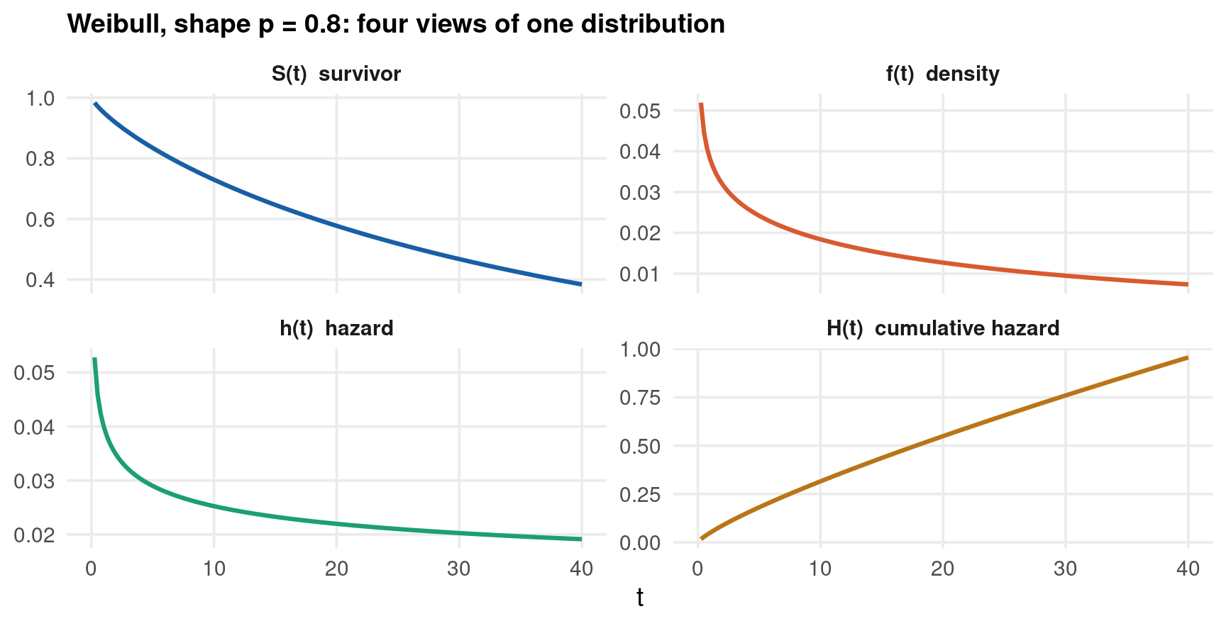
Code
import numpy as np
import matplotlib.pyplot as plt

p, lam = 0.8, 0.05
t = np.arange(0.25, 40.01, 0.25)

S = np.exp(-lam * t**p)
h = p * lam * t**(p - 1)
f = h * S
H = lam * t**p

curves = [("S(t)  survivor", S, "#185FA5"), ("f(t)  density", f, "#D85A30"),
          ("h(t)  hazard", h, "#1D9E75"), ("H(t)  cumulative hazard", H, "#BA7517")]

fig, axes = plt.subplots(2, 2, figsize=(9, 4.6))
for ax, (name, y, col) in zip(axes.ravel(), curves):
    ax.plot(t, y, color=col, lw=1.8)
    axopts = ax.set(xlim=(0, 40), xticks=range(0, 41, 10), title=name, xlabel="t")
fig.suptitle("Weibull, shape p = 0.8: four views of one distribution")
fig.tight_layout()
plt.show()
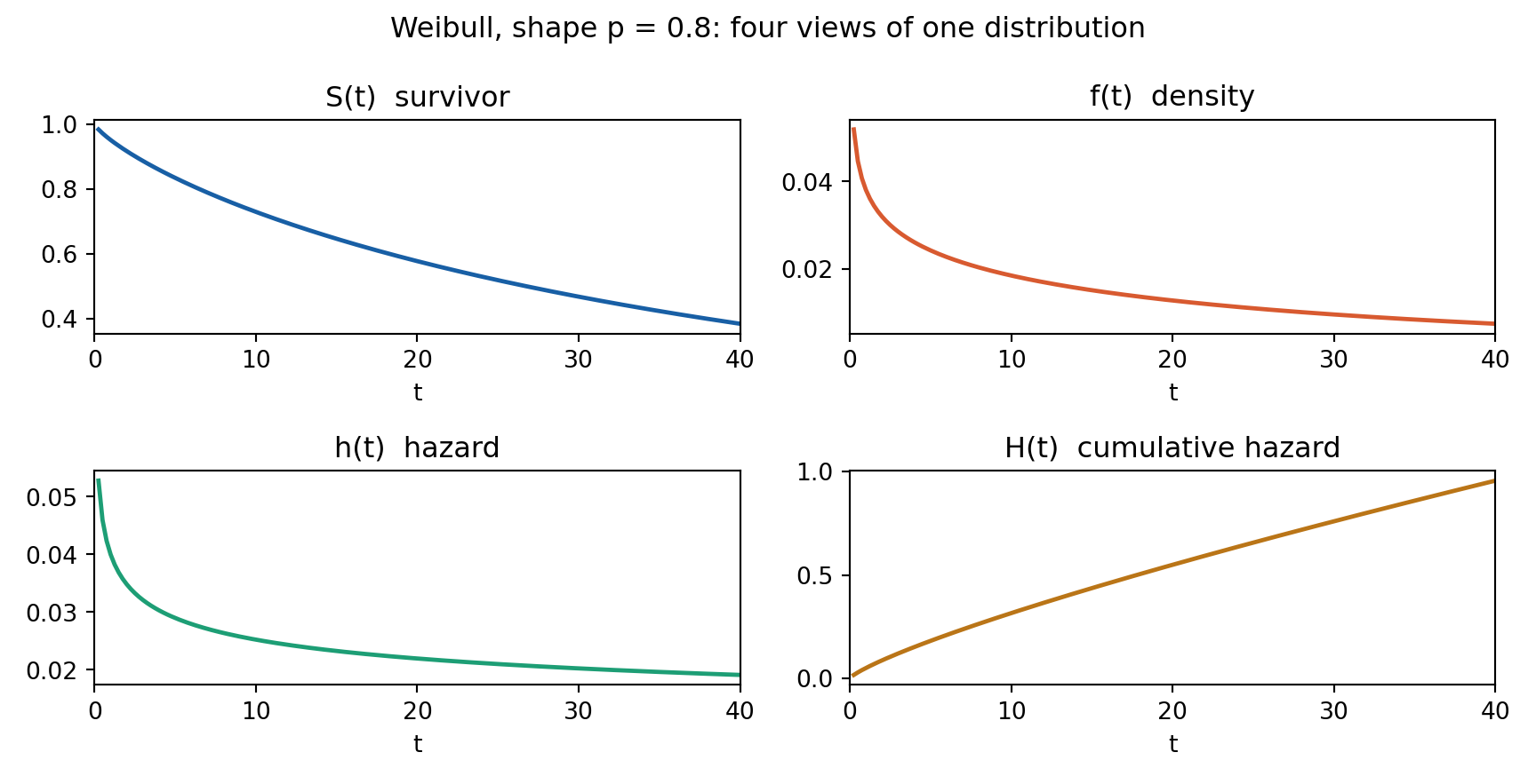
Code
clear
set obs 160
gen t = 0.25 * _n
gen S = exp(-0.05 * t^0.8)
gen h = 0.8 * 0.05 * t^(0.8 - 1)
gen f = h * S
gen H = 0.05 * t^0.8

twoway line S t, lcolor("24 95 165") lwidth(medthick)                         ///
    xscale(range(0 40)) xlabel(0(10)40) xtitle("t") ytitle("")                ///
    title("S(t)  survivor", size(medium))                                     ///
    graphregion(color(white)) plotregion(color(white)) name(g1, replace)
twoway line f t, lcolor("216 90 48") lwidth(medthick)                         ///
    xscale(range(0 40)) xlabel(0(10)40) xtitle("t") ytitle("")                ///
    title("f(t)  density", size(medium))                                      ///
    graphregion(color(white)) plotregion(color(white)) name(g2, replace)
twoway line h t, lcolor("29 158 117") lwidth(medthick)                        ///
    xscale(range(0 40)) xlabel(0(10)40) xtitle("t") ytitle("")                ///
    title("h(t)  hazard", size(medium))                                       ///
    graphregion(color(white)) plotregion(color(white)) name(g3, replace)
twoway line H t, lcolor("186 117 23") lwidth(medthick)                        ///
    xscale(range(0 40)) xlabel(0(10)40) xtitle("t") ytitle("")                ///
    title("H(t)  cumulative hazard", size(medium))                            ///
    graphregion(color(white)) plotregion(color(white)) name(g4, replace)

graph combine g1 g2 g3 g4, cols(2) graphregion(color(white))                  ///
    title("Weibull, shape p = 0.8: four views of one distribution", size(medsmall)) ///
    xsize(9) ysize(4.6)
graph export "../plots/dsc-p1-four.png", replace width(1800)
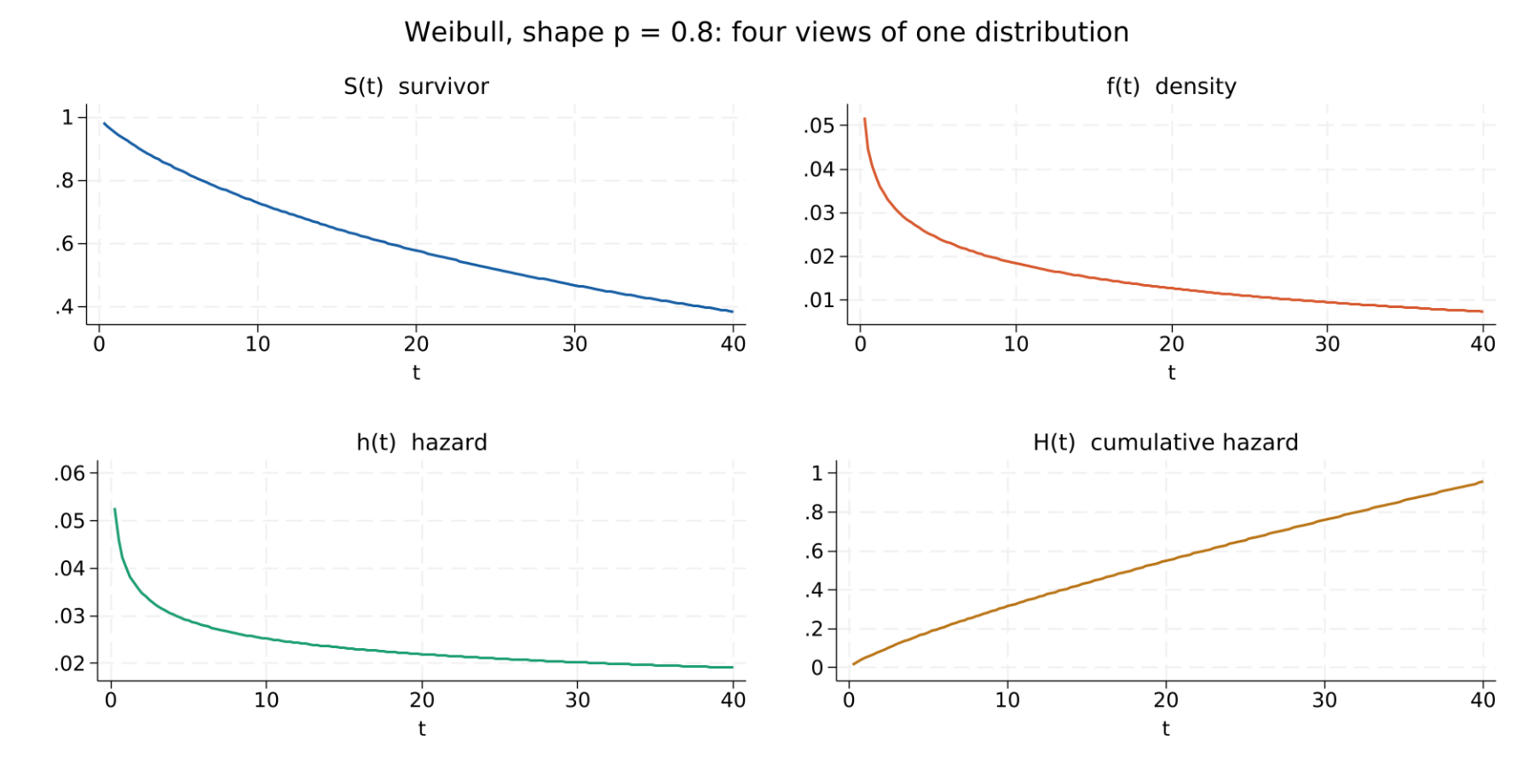
Why the Hazard Is the Interesting One

Of the four, only the hazard is something an economic agent chooses.

A search model delivers the re-employment hazard directly. Let \(\lambda\) be the rate at which offers arrive and \(F_w\) the wage-offer distribution. A worker with reservation wage \(w^R\) accepts an offer if it exceeds \(w^R\), so

\[h(t) = \lambda \cdot \Pr(w > w^R_t) = \lambda \big[1 - F_w(w^R_t)\big]\]

Every term is a primitive of the model. The hazard is the re-employment probability per unit time, and the comparative statics land on it cleanly:

  • a benefit extension raises \(w^R\), so the hazard falls
  • a tighter labour market raises \(\lambda\), so the hazard rises
  • benefit exhaustion at week 26 makes \(w^R\) drop discretely, so the hazard should spike at 26 — a prediction visible in raw data, and one of the best-identified findings in the literature

\(S(t)\) and \(f(t)\) are unconditional: they describe the original cohort. The hazard conditions on still being at risk, which is the only population you can actually observe at \(t\).

That makes it the natural target for time-varying covariates. A benefit change in month 12 can only affect people still unemployed in month 12, and \(h(12)\) is defined on exactly that group. Writing the same statement in terms of \(S\) or \(f\) means carrying the entire history along.

The hazard estimated from data is a hazard averaged over the survivors, not the hazard of a representative individual. The two coincide only if everyone is identical. Part 5 shows that they routinely diverge in sign.

A second, smaller trap: a hazard ratio is a ratio of rates, not of durations. A hazard ratio of 1.5 does not mean spells are 50% shorter. The translation depends on the whole shape of the baseline, and Part 3 does it properly.

Duration Dependence

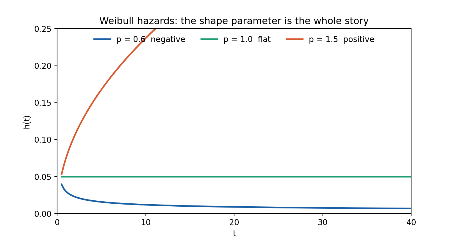
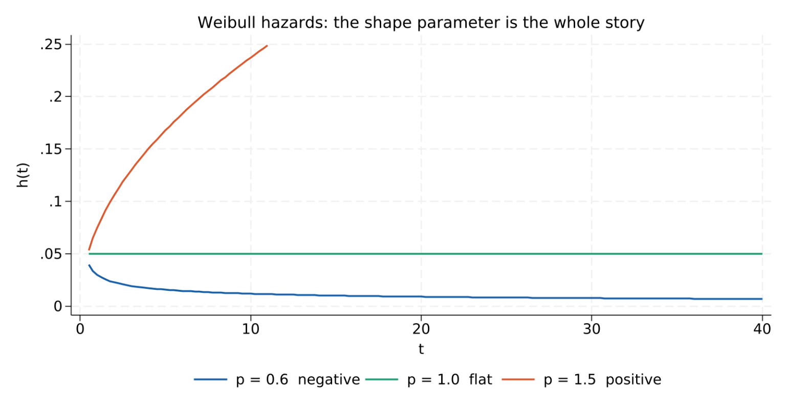
\[\text{positive duration dependence: } \frac{\partial h(t)}{\partial t} > 0 \qquad \text{negative: } \frac{\partial h(t)}{\partial t} < 0\]

Negative — the longer you have waited, the less likely you are to exit now. Behavioural stories: skills depreciate, employers read long unemployment as a bad signal, discouragement sets in, network contacts go stale.

Positive — the longer you have waited, the more likely to exit now. Stories: benefits run out, savings are exhausted, a fixed-term contract approaches its end, a machine wears out.

Flat (\(h\) constant) — the exponential case, and the memoryless one. How long you have already waited tells you nothing about what happens next. It is the natural null hypothesis, and Part 4 tests it as \(p = 1\) in a Weibull.

For the Weibull the whole question reduces to one parameter:

\[h(t) = p\,\lambda\, t^{\,p-1} \quad\Longrightarrow\quad \begin{cases} p < 1 & \text{negative duration dependence}\\ p = 1 & \text{constant hazard (exponential)}\\ p > 1 & \text{positive duration dependence} \end{cases}\]

which is why \(\hat{p}\) and its standard error are the first things to read off a Weibull fit — and why Part 5 spends eight slides on the fact that \(\hat p < 1\) is not evidence of negative duration dependence.

Code
t <- seq(0.5, 40, by = 0.25)
lambda <- 0.05

dd <- data.frame(
  t = rep(t, 3),
  h = c(0.6 * lambda * t^(0.6 - 1),
        1.0 * lambda * t^(1.0 - 1),
        1.5 * lambda * t^(1.5 - 1)),
  shape = factor(rep(c("p = 0.6  negative", "p = 1.0  flat",
                       "p = 1.5  positive"), each = length(t)))
)

ggplot(dd) +
  aes(x = t, y = h, colour = shape) +
  geom_line(linewidth = 1.2) +
  scale_colour_manual(values = c("#185FA5", "#1D9E75", "#D85A30")) +
  coord_cartesian(xlim = c(0, 40), ylim = c(0, 0.25)) +
  scale_x_continuous(breaks = seq(0, 40, 10)) +
  scale_y_continuous(breaks = seq(0, 0.25, 0.05)) +
  labs(x = "t", y = "h(t)", colour = NULL,
       title = "Weibull hazards: the shape parameter is the whole story")
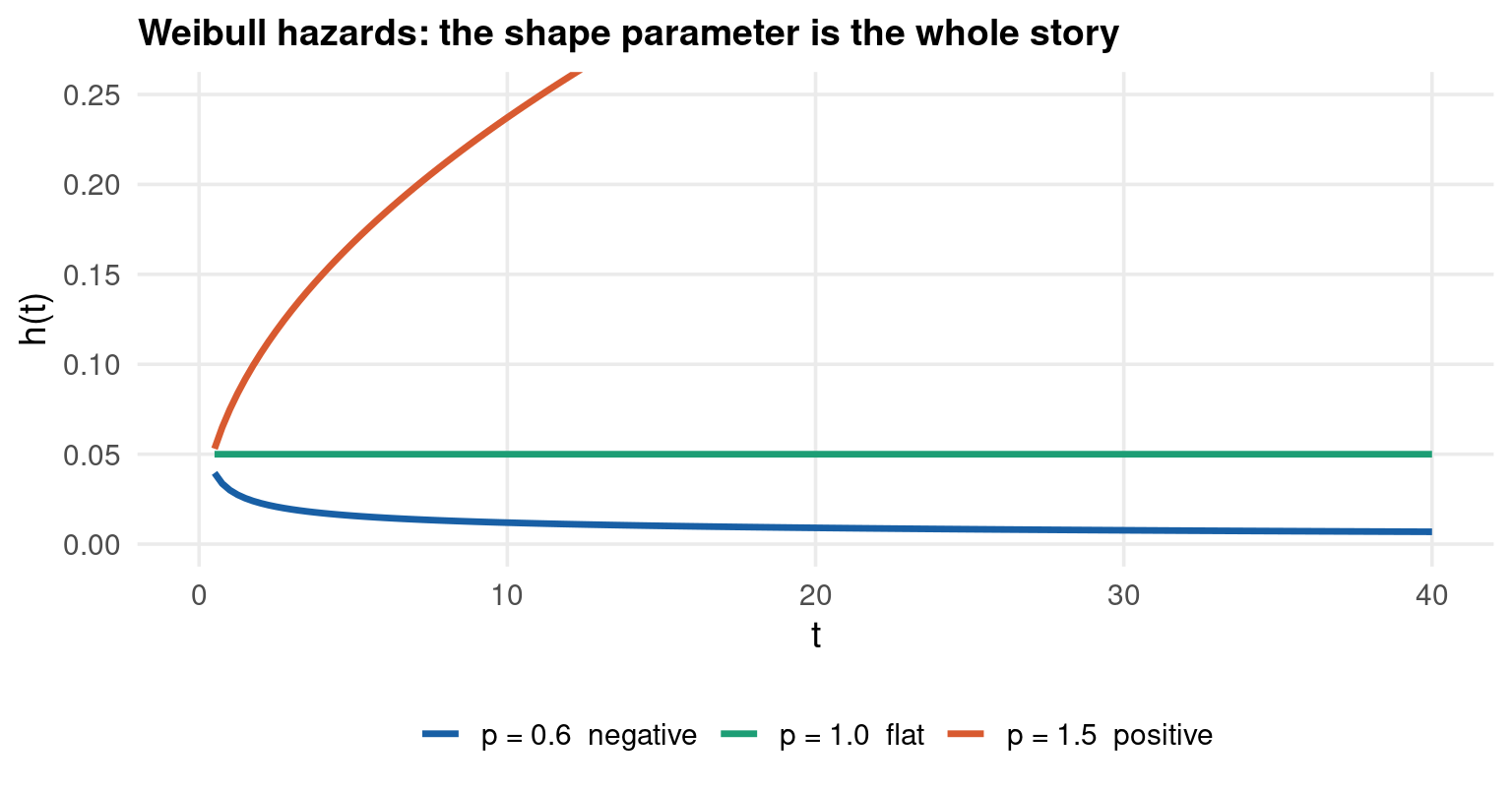
Code
import numpy as np
import matplotlib.pyplot as plt

t, lam = np.arange(0.5, 40.01, 0.25), 0.05
shapes = [(0.6, "p = 0.6  negative", "#185FA5"),
          (1.0, "p = 1.0  flat",     "#1D9E75"),
          (1.5, "p = 1.5  positive", "#D85A30")]

fig, ax = plt.subplots(figsize=(8, 4.2))
for p, lab, col in shapes:
    ax.plot(t, p * lam * t**(p - 1), color=col, lw=2, label=lab)
axopts = ax.set(xlim=(0, 40), ylim=(0, 0.25), xticks=range(0, 41, 10),
                yticks=np.arange(0, 0.26, 0.05), xlabel="t", ylabel="h(t)",
                title="Weibull hazards: the shape parameter is the whole story")
ax.legend(loc="upper center", ncol=3, frameon=False)
plt.show()
Code
clear
set obs 159
gen t = 0.25 + 0.25 * _n
gen h06 = 0.6 * 0.05 * t^(0.6 - 1)
gen h10 = 1.0 * 0.05 * t^(1.0 - 1)
gen h15 = 1.5 * 0.05 * t^(1.5 - 1)

* yscale(range()) only EXTENDS a Stata axis, it never clips, so the p = 1.5
* curve has to be restricted by hand to match ggplot's coord_cartesian
twoway (line h06 t if h06 <= 0.25, lcolor("24 95 165")  lwidth(medthick))     ///
       (line h10 t if h10 <= 0.25, lcolor("29 158 117") lwidth(medthick))     ///
       (line h15 t if h15 <= 0.25, lcolor("216 90 48")  lwidth(medthick)),    ///
    legend(order(1 "p = 0.6  negative" 2 "p = 1.0  flat"                      ///
                 3 "p = 1.5  positive") rows(1) position(6) ring(1) region(lstyle(none)))         ///
    xscale(range(0 40)) xlabel(0(10)40)                                       ///
    yscale(range(0 0.25)) ylabel(0(0.05)0.25)                                 ///
    xtitle("t") ytitle("h(t)")                                                ///
    title("Weibull hazards: the shape parameter is the whole story", size(medium)) ///
    graphregion(color(white)) plotregion(color(white)) xsize(8) ysize(4.2)
graph export "../plots/dsc-p1-dd.png", replace width(1600)
Literature

  • Lancaster (1979) — the paper that brought hazard models into unemployment econometrics, and the first clear statement of the frailty problem in economics. 10.2307/1914140
  • Elbers & Ridder (1982) — identification of the mixed proportional hazard model; the result Part 5 rests on. 10.2307/2297364
  • Heckman & Singer (1984) — how badly the frailty distribution matters, and the nonparametric alternative. 10.2307/1911491
  • Meyer (1990) — unemployment insurance and the spike at benefit exhaustion; the empirical benchmark. 10.2307/2938349
  • van den Berg (2001) — the Handbook of Econometrics chapter; the best single survey for economists. 10.1016/S1573-4412(01)05008-5
  • Prentice & Gloeckler (1978) — grouped-duration data and the complementary log-log hazard; the bridge to panel binary models. 10.2307/2529588
  • Han & Hausman (1990) — flexible discrete-time estimation of the proportional hazard, in an econometrics idiom. 10.1002/jae.3950050102
  • Fine & Gray (1999) — the subdistribution hazard; the reason “cause-specific or subdistribution?” is a real question. 10.1080/01621459.1999.10474144
  • Gouriéroux, Monfort & Trognon (1984) — pseudo-maximum likelihood; why Poisson survives its own misspecification. 10.2307/1913472
  • Hausman, Hall & Griliches (1984) — count panels, patents and R&D; the origin of fixed-effects Poisson in economics. 10.2307/1911191
  • Mullahy (1986) — hurdle models; the two-part story for zeros. 10.1016/0304-4076(86)90002-3
  • Cameron & Trivedi (1990) — regression-based tests for overdispersion; the test used in Part 7. 10.1016/0304-4076(90)90014-K
  • Lambert (1992) — zero-inflated Poisson. 10.2307/1269547
  • Wilson (2015) — why the Vuong test should not be used to choose zero-inflation. 10.1016/j.econlet.2014.12.029
  • Wooldridge (2010), Econometric Analysis of Cross Section and Panel Data, 2nd ed., MIT Press — Ch. 18 (counts) and Ch. 22 (duration); the source of recid and crime1.
  • Cameron & Trivedi (2013), Regression Analysis of Count Data, 2nd ed., Cambridge UP. 10.1017/CBO9781139013567
  • Cleves, Gould & Marchenko (2016), An Introduction to Survival Analysis Using Stata, 3rd ed., Stata Press — the best applied companion to the st suite.
  • Jenkins (2005), Survival Analysis, lecture notes, University of Essex — the standard free reference for economists. iser.essex.ac.uk/files/teaching/stephenj/ec968

Part 2 — Nonparametric Survival

Kaplan–Meier, Nelson–Aalen, and the log-rank test

The Risk Set

Everything nonparametric in survival analysis comes from a single move: condition on the risk set.

\[R(t) = \{\, i : t_i \ge t \,\}, \qquad n_t = |R(t)|\]

\(R(t)\) is the set of units still under observation and still event-free just before \(t\). At an observed event time \(t_{(j)}\) you know two integers, and nothing else needs assuming:

\[d_j = \text{events at } t_{(j)}, \qquad n_j = \text{units at risk just before } t_{(j)}\]

The conditional probability of failing at \(t_{(j)}\) given survival up to it is estimated by the obvious sample proportion, \(d_j / n_j\). Kaplan–Meier multiplies these, Nelson–Aalen adds them, the log-rank test compares them across groups. No distribution, no functional form, no covariates.

A censored observation stays in the risk set for as long as it is observed and then leaves without ever contributing an event. It shrinks \(n_j\) for all later \(j\), and that is its entire effect.

This is why the estimator is not the empirical survivor function of the observed \(t_i\). That naive object treats a censored spell as if it had ended, biasing survival downward. The product-limit estimator treats it as if it had continued, with unknown length — which is the truth.

Convention when a censoring time equals an event time: events first. The censored unit is counted in \(n_j\) for that event and removed afterwards. All three languages do this, and it matters when durations are recorded in coarse units — which is exactly the recid case, where time is whole months.

Buys — consistency for \(S(t)\) under nothing more than independent censoring, and a picture any audience can read.

Costs — it is a marginal description. There are no covariates, so it cannot answer “holding age constant”. Groups can be compared only by splitting the sample, which runs out of data quickly: two binary covariates already mean four curves, four binary covariates mean sixteen.

That limitation is precisely what Part 3 removes.

Kaplan–Meier

Order the distinct event times \(t_{(1)} < t_{(2)} < \cdots < t_{(k)}\). The survivor function is estimated by chaining conditional survival probabilities:

\[\hat{S}(t) = \prod_{j:\, t_{(j)} \le t} \left( 1 - \frac{d_j}{n_j} \right)\]

It is a step function — flat between event times, dropping only where an event occurs. Censoring times produce no step; they only thin the risk set.

It is also the nonparametric maximum-likelihood estimator of \(S\) under independent censoring, so this is not a convenient recipe but the estimator.

\[\widehat{\mathrm{Var}}\big[\hat{S}(t)\big] = \hat{S}(t)^2 \sum_{j:\, t_{(j)} \le t} \frac{d_j}{n_j\,(n_j - d_j)}\]

Confidence intervals built directly from this are symmetric and can leave \([0,1]\) in the tails. Every language therefore defaults to a transformed interval, usually on the \(\log(-\log S)\) scale, which respects the bounds:

\[\log\{-\log \hat{S}(t)\} \;\pm\; z_{\alpha/2}\, \frac{\sqrt{\widehat{\mathrm{Var}}[\hat S(t)]}}{\hat{S}(t)\,\big|\log \hat{S}(t)\big|}\]

R’s survfit, Stata’s sts and lifelines all use this transformation by default. That is why the three sets of bands on the slide after next agree rather than merely resemble one another.

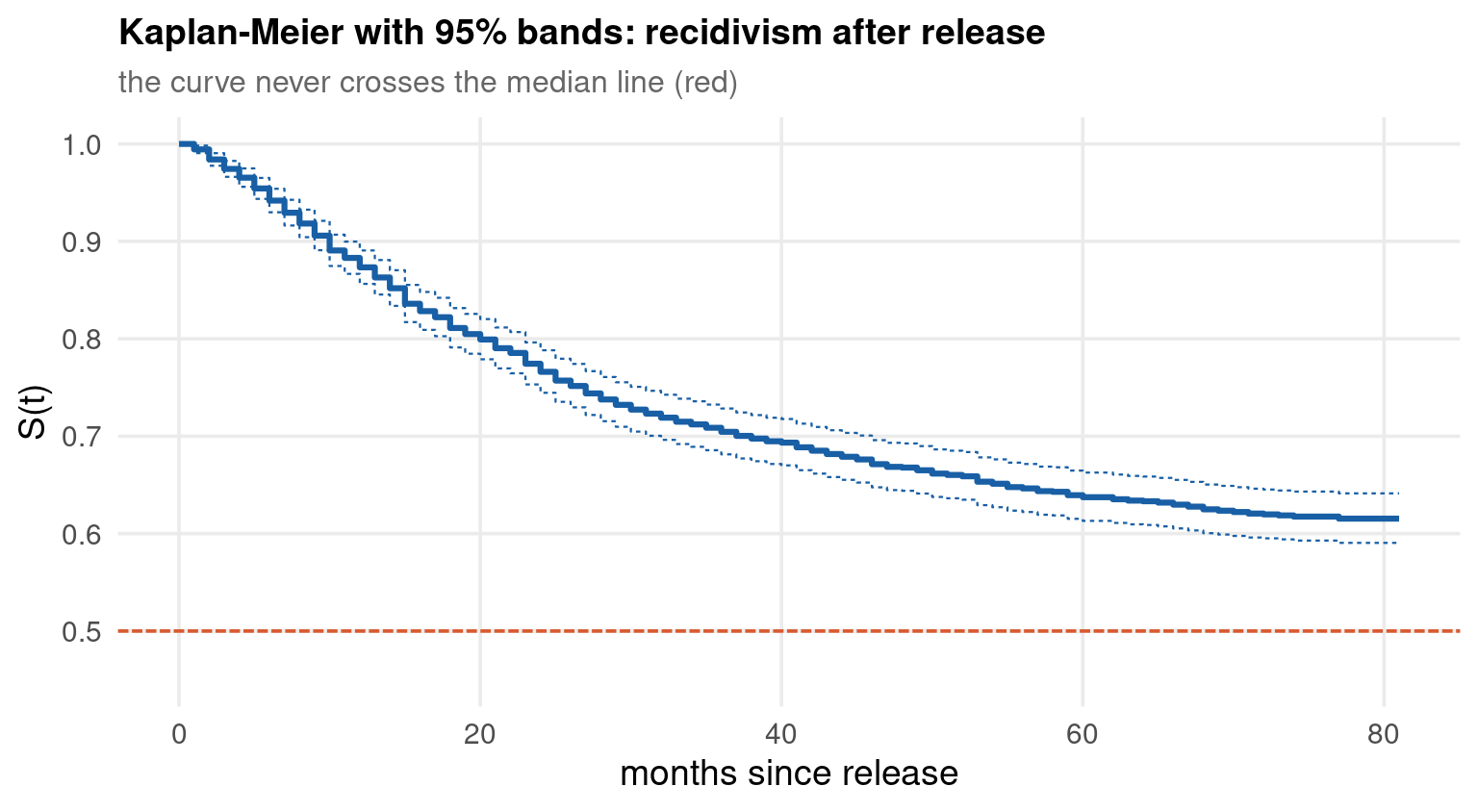
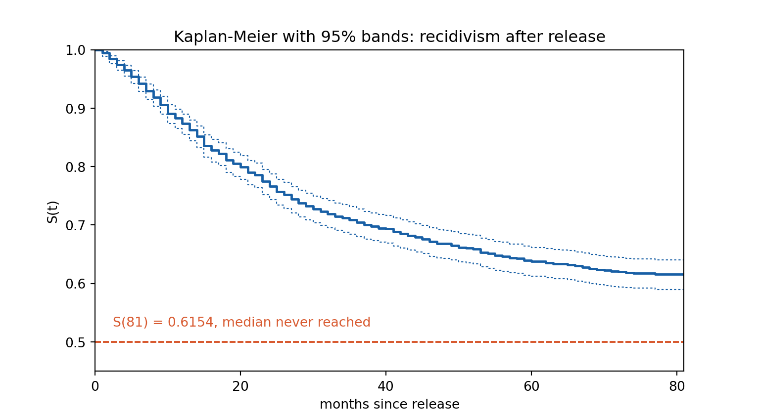
The median survival time is \(\hat{t}_{0.5} = \inf\{t : \hat{S}(t) \le 0.5\}\), and if \(\hat{S}\) never reaches \(0.5\) then it is not estimable.

In recid only 38% of the men return to prison, so \(\hat{S}\) bottoms out at \(0.6154\) and the median is undefined. R prints NA, lifelines prints inf, Stata leaves the cell blank. None of them is broken.

Reporting “mean duration = 55.4 months” from recid — the sample mean of durat — is simply wrong: it averages 552 real durations together with 893 lower bounds. When the median is not reached, report \(\hat{S}(t)\) at fixed, policy-relevant horizons instead. That is the honest summary, and it is what the next slide does.

Kaplan–Meier on recid

The same 1445 men, three languages, native loads. The first three numbers are the censoring parity check: if the event indicator is built differently anywhere, these integers diverge and every curve after this slide is wrong.

Code
library(survival)
data("recid", package = "wooldridge")

# cens == 1 marks a spell still running when the study window closed,
# so the EVENT indicator is its complement.
recid <- transform(recid, fail = 1 - cens)

cat("n =", nrow(recid),
    " events =", sum(recid$fail), " censored =", sum(1 - recid$fail), "\n\n")

km <- survfit(Surv(durat, fail) ~ 1, data = recid)

s <- summary(km, times = c(12, 24, 36, 48, 60))
out <- data.frame(months = s$time, at_risk = s$n.risk, events = s$n.event,
                  S = round(s$surv, 4),
                  lower = round(s$lower, 4), upper = round(s$upper, 4))
print(out, row.names = FALSE)

cat("\nmedian survival:", summary(km)$table["median"],
    "  (NA = never reached; S bottoms out at", round(min(km$surv), 4), ")\n")
n = 1445  events = 552  censored = 893 
 months at_risk events      S  lower  upper
     12    1276    183 0.8734 0.8564 0.8907
     24    1119    155 0.7661 0.7446 0.7882
     36    1024     89 0.7045 0.6814 0.7284
     48     966     53 0.6678 0.6440 0.6926
     60     924     44 0.6374 0.6131 0.6626

median survival: NA   (NA = never reached; S bottoms out at 0.6154 )
Code
import numpy as np
import pandas as pd
import wooldridge as woo
from lifelines import KaplanMeierFitter

rc = woo.data('recid')
# cens == 1 marks a spell still running when the study window closed.
rc = rc.assign(fail=1 - rc['cens'])

lines = ["n = %d  events = %d  censored = %d\n" %
         (len(rc), int(rc['fail'].sum()), int((1 - rc['fail']).sum()))]

km = KaplanMeierFitter().fit(rc['durat'], rc['fail'])
ci = km.confidence_interval_

rows = []
for t in [12, 24, 36, 48, 60]:
    at_risk = int((rc['durat'] >= t).sum())
    lo, hi = ci[ci.index <= t].iloc[-1]
    rows.append((t, at_risk, round(float(km.predict(t)), 4),
                 round(float(lo), 4), round(float(hi), 4)))

tab = pd.DataFrame(rows, columns=["months", "at_risk", "S", "lower", "upper"])
lines.append(tab.to_string(index=False))
lines.append("\nmedian survival: %s  (inf = never reached; S bottoms out at %.4f)"
             % (km.median_survival_time_, float(km.survival_function_.iloc[-1, 0])))

import sys
nw = sys.stdout.write("\n".join(lines) + "\n")
n = 1445  events = 552  censored = 893

 months  at_risk      S  lower  upper
     12     1276 0.8734 0.8551 0.8895
     24     1119 0.7661 0.7434 0.7871
     36     1024 0.7045 0.6802 0.7273
     48      966 0.6678 0.6429 0.6915
     60      924 0.6374 0.6120 0.6616

median survival: inf  (inf = never reached; S bottoms out at 0.6154)
Code
sys.stdout.flush()
Code
quietly frause recid, clear
* cens == 1 marks a spell still running when the study window closed.
gen fail = 1 - cens
count
count if fail == 1
count if fail == 0
stset durat, failure(fail == 1)
sts list, at(12 24 36 48 60)
stci
  1,445

  552

  893


Survival-time data settings

         Failure event: fail==1
Observed time interval: (0, durat]
     Exit on or before: failure

--------------------------------------------------------------------------
      1,445  total observations
          0  exclusions
--------------------------------------------------------------------------
      1,445  observations remaining, representing
        552  failures in single-record/single-failure data
     80,013  total analysis time at risk and under observation
                                                At risk from t =         0
                                     Earliest observed entry t =         0
                                          Last observed exit t =        81

        Failure _d: fail==1
  Analysis time _t: durat

Kaplan–Meier survivor function

              Beg.             Survivor      Std.
    Time     total     Fail    function     error     [95% conf. int.]
----------------------------------------------------------------------
      12      1276      183      0.8734    0.0087     0.8551    0.8895
      24      1119      155      0.7661    0.0111     0.7434    0.7871
      36      1024       89      0.7045    0.0120     0.6802    0.7273
      48       966       53      0.6678    0.0124     0.6429    0.6915
      60       924       44      0.6374    0.0126     0.6120    0.6616
----------------------------------------------------------------------
Note: Survivor function is calculated over full data and evaluated at
      indicated times; it is not calculated from aggregates shown at left.

        Failure _d: fail==1
  Analysis time _t: durat

             | Number of 
             |  subjects         50%      Std. err.    [95% conf. interval]
-------------+-------------------------------------------------------------
       Total |      1445           .             .            .          .

Parity confirmed. All three report 1445 men, 552 events and 893 censored spells, with \(\hat{S}(12) = 0.8734\), \(\hat{S}(36) = 0.7045\) and \(\hat{S}(60) = 0.6374\). The median is not reached in any of them.

The Curve, with Confidence Bands

Code
data("recid", package = "wooldridge")
recid <- transform(recid, fail = 1 - cens)
km <- survfit(Surv(durat, fail) ~ 1, data = recid)

curve <- data.frame(t = c(0, km$time), S = c(1, km$surv),
                    lo = c(1, km$lower), hi = c(1, km$upper))

# geom_step, never geom_line: the estimator IS a step function
ggplot(curve) +
  aes(x = t, y = S) +
  geom_step(colour = "#185FA5", linewidth = 1.1) +
  geom_step(aes(y = lo), colour = "#185FA5", linewidth = 0.4, linetype = "22") +
  geom_step(aes(y = hi), colour = "#185FA5", linewidth = 0.4, linetype = "22") +
  geom_hline(yintercept = 0.5, colour = "#D85A30", linetype = "31") +
  coord_cartesian(xlim = c(0, 81), ylim = c(0.45, 1)) +
  scale_x_continuous(breaks = seq(0, 80, 20)) +
  scale_y_continuous(breaks = seq(0.5, 1, 0.1)) +
  labs(x = "months since release", y = "S(t)",
       title = "Kaplan-Meier with 95% bands: recidivism after release",
       subtitle = "the curve never crosses the median line (red)")
Code
import numpy as np
import matplotlib.pyplot as plt
import wooldridge as woo
from lifelines import KaplanMeierFitter

rc = woo.data('recid').assign(fail=lambda d: 1 - d['cens'])
km = KaplanMeierFitter().fit(rc['durat'], rc['fail'])

t  = km.survival_function_.index.values
S  = km.survival_function_.iloc[:, 0].values
lo = km.confidence_interval_.iloc[:, 0].values
hi = km.confidence_interval_.iloc[:, 1].values

fig, ax = plt.subplots(figsize=(8, 4.4))
# steps-post, never a smooth line
ax.step(t, S,  where="post", color="#185FA5", lw=1.8)
ax.step(t, lo, where="post", color="#185FA5", lw=0.8, ls=(0, (2, 2)))
ax.step(t, hi, where="post", color="#185FA5", lw=0.8, ls=(0, (2, 2)))
ax.axhline(0.5, color="#D85A30", ls=(0, (3, 1)))
ax.text(0.03, 0.14, "S(81) = %.4f, median never reached" % S[-1],
        transform=ax.transAxes, fontsize=10, color="#D85A30")
axopts = ax.set(xlim=(0, 81), ylim=(0.45, 1.0), xticks=range(0, 81, 20),
                yticks=np.arange(0.5, 1.01, 0.1),
                xlabel="months since release", ylabel="S(t)",
                title="Kaplan-Meier with 95% bands: recidivism after release")
plt.show()
Code
quietly frause recid, clear
gen fail = 1 - cens
quietly stset durat, failure(fail == 1)

sts graph, ci                                                                 ///
    plotopts(lcolor("24 95 165") lwidth(medthick))                            ///
    ciopts(color("24 95 165%25"))                                             ///
    yline(0.5, lcolor("216 90 48") lpattern(dash))                            ///
    xscale(range(0 81)) xlabel(0(20)80)                                       ///
    yscale(range(0.45 1)) ylabel(0.5(0.1)1)                                   ///
    xtitle("months since release") ytitle("S(t)")                             ///
    title("Kaplan-Meier with 95% bands: recidivism after release", size(medium)) ///
    subtitle("the curve never crosses the median line (red)", size(small))    ///
    legend(off) graphregion(color(white)) plotregion(color(white))            ///
    xsize(8) ysize(4.4)
graph export "../plots/dsc-p2-km.png", replace width(1600)
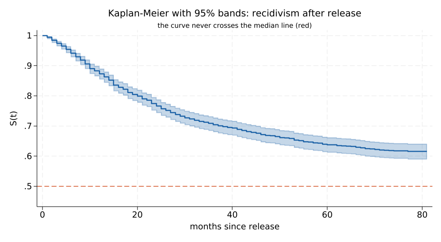
The curve falls steeply through the first year — \(\hat{S}\) drops from \(1\) to \(0.8734\) by month 12 — and then flattens. Read that shape carefully: it is either genuine negative duration dependence or a mix of high- and low-risk men sorting themselves out over time. Nothing on this slide distinguishes the two, and Part 5 is about how often that distinction gets skipped.

Nelson–Aalen and the Cumulative Hazard

Where Kaplan–Meier multiplies, Nelson–Aalen adds:

\[\hat{H}(t) = \sum_{j:\, t_{(j)} \le t} \frac{d_j}{n_j}, \qquad \widehat{\mathrm{Var}}\big[\hat H(t)\big] = \sum_{j:\, t_{(j)} \le t} \frac{d_j}{n_j^{2}}\]

The two are two views of one object: \(\hat{S}_{\text{FH}}(t) = \exp\{-\hat{H}(t)\}\) is the Fleming–Harrington survivor estimate, and it agrees with Kaplan–Meier to within \(O(d_j^2/n_j^2)\) — indistinguishable unless the risk set gets small.

Because the slope of \(\hat H\) is the hazard, and slopes are much easier to read off a picture than curvature:

\[\frac{d\hat{H}(t)}{dt} \approx h(t)\]

Shape of \(\hat H(t)\) Slope Duration dependence
straight line constant none — exponential
concave (bends down) falling negative
convex (bends up) rising positive

A glance at \(\hat H\) therefore does what a glance at \(\hat S\) cannot: it separates a constant hazard from a declining one. It is the standard pre-modelling diagnostic, and it is what motivates the family choice in Part 4.

Code
data("recid", package = "wooldridge")
recid <- transform(recid, fail = 1 - cens)

na <- survfit(Surv(durat, fail) ~ 1, data = recid, type = "fleming-harrington")
H  <- data.frame(t = c(0, na$time), H = c(0, -log(na$surv)))

s <- summary(na, times = c(12, 24, 36, 48, 60, 80))
print(data.frame(months = s$time, H = round(-log(s$surv), 4)), row.names = FALSE)

ggplot(H) +
  aes(x = t, y = H) +
  geom_step(colour = "#1D9E75", linewidth = 1.1) +
  geom_abline(intercept = 0, slope = 0.483295 / 80,
              colour = "#D85A30", linetype = "31") +
  coord_cartesian(xlim = c(0, 81), ylim = c(0, 0.55)) +
  scale_x_continuous(breaks = seq(0, 80, 20)) +
  scale_y_continuous(breaks = seq(0, 0.5, 0.1)) +
  labs(x = "months since release", y = "H(t)",
       title = "Nelson-Aalen cumulative hazard",
       subtitle = "concave against the constant-hazard ray: the hazard is falling")
 months      H
     12 0.1346
     24 0.2649
     36 0.3484
     48 0.4017
     60 0.4482
     80 0.4833
Code
import numpy as np
import matplotlib.pyplot as plt
import wooldridge as woo
from lifelines import NelsonAalenFitter

rc = woo.data('recid').assign(fail=lambda d: 1 - d['cens'])
na = NelsonAalenFitter().fit(rc['durat'], rc['fail'])

t = np.r_[0.0, na.cumulative_hazard_.index.values]
H = np.r_[0.0, na.cumulative_hazard_.iloc[:, 0].values]

fig, ax = plt.subplots(figsize=(8, 4.2))
ax.step(t, H, where="post", color="#1D9E75", lw=1.8)
ax.plot([0, 80], [0, 0.483295], color="#D85A30", ls=(0, (3, 1)))
ax.text(0.03, 0.86, "H(12) = %.4f    H(36) = %.4f    H(60) = %.4f"
        % (np.interp(12, t, H), np.interp(36, t, H), np.interp(60, t, H)),
        transform=ax.transAxes, fontsize=10, color="#1D9E75")
axopts = ax.set(xlim=(0, 81), ylim=(0, 0.55), xticks=range(0, 81, 20),
                yticks=np.arange(0, 0.51, 0.1),
                xlabel="months since release", ylabel="H(t)",
                title="Nelson-Aalen cumulative hazard")
plt.show()
Code
quietly frause recid, clear
gen fail = 1 - cens
quietly stset durat, failure(fail == 1)
quietly sts gen H = na
quietly gen ray = 0.483295 * durat / 80

twoway (line H durat, connect(stairstep) sort lcolor("29 158 117") lwidth(medthick)) ///
       (line ray durat, sort lcolor("216 90 48") lpattern(dash)),                    ///
    xscale(range(0 81)) xlabel(0(20)80)                                              ///
    yscale(range(0 0.55)) ylabel(0(0.1)0.5)                                          ///
    xtitle("months since release") ytitle("H(t)")                                    ///
    title("Nelson-Aalen cumulative hazard", size(medium))                            ///
    subtitle("concave against the constant-hazard ray: the hazard is falling", size(small)) ///
    legend(off) graphregion(color(white)) plotregion(color(white))                   ///
    xsize(8) ysize(4.2)
graph export "../plots/dsc-p2-na.png", replace width(1600)
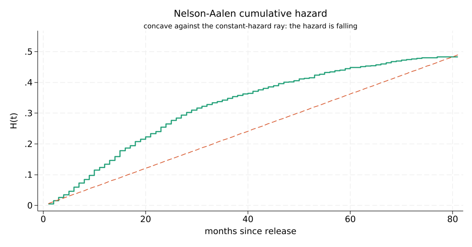
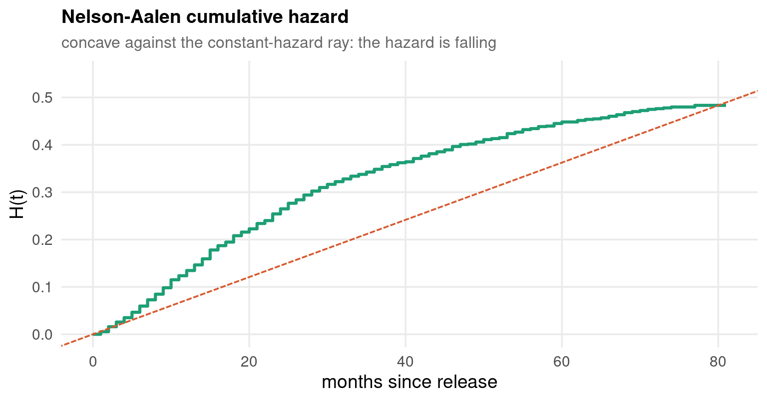
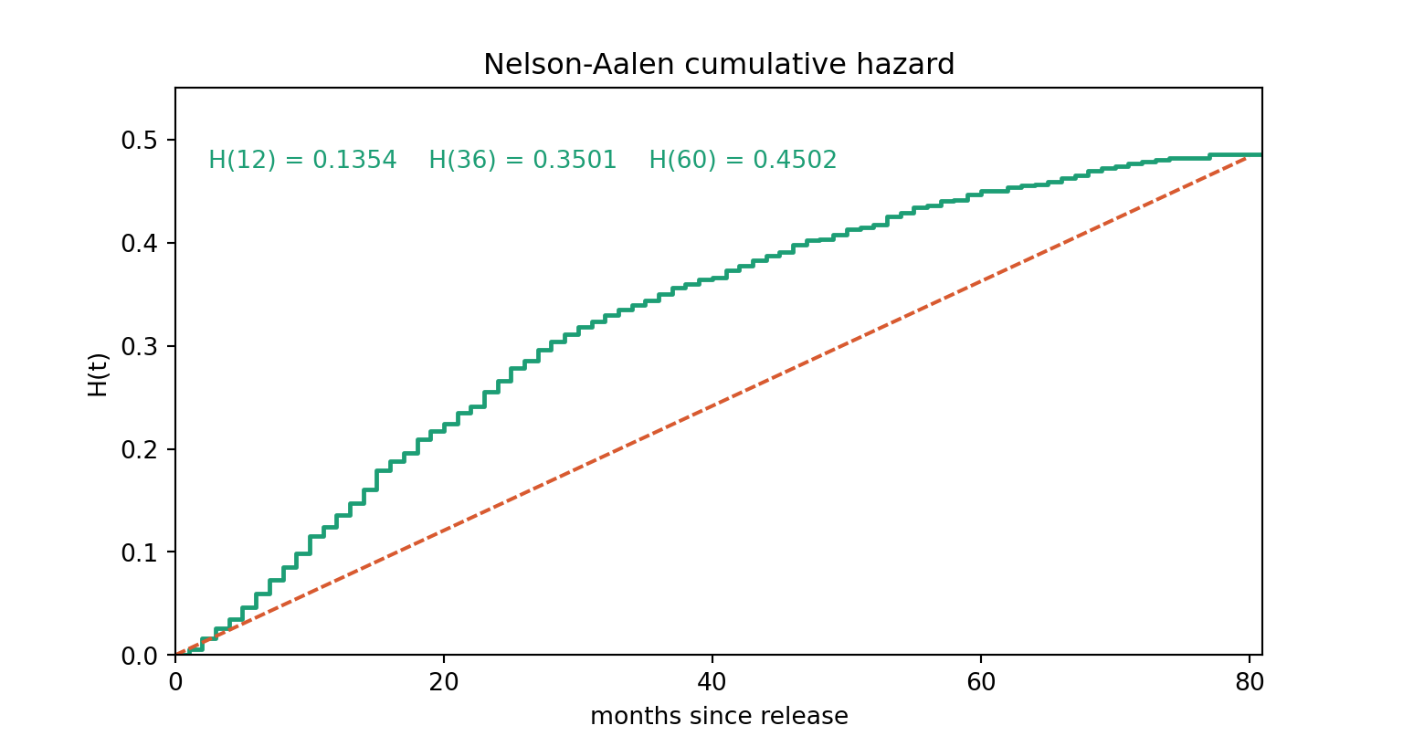
\(\hat H\) reaches \(0.1346\) by month 12 but only \(0.4833\) by month 80: the first year alone accounts for 28% of the risk accumulated over nearly seven years. The curve sits above the straight ray early and falls below it later — visibly concave, so the observed hazard is falling.

The Log-Rank Test

The question is whether two survivor functions are the same, without assuming anything about their shape:

\[H_0: S_1(t) = S_2(t) \quad \text{for all } t\]

At each event time \(t_{(j)}\) build the \(2\times2\) table of group by outcome. Under \(H_0\), conditional on the margins, the number of events in group 1 is hypergeometric:

\[E_{1j} = d_j\,\frac{n_{1j}}{n_j}, \qquad V_j = \frac{n_{1j}\,n_{2j}\,d_j\,(n_j - d_j)}{n_j^{2}\,(n_j - 1)}\]

Sum observed minus expected across event times and standardise:

\[\chi^2_{\text{LR}} = \frac{\left(\sum_j d_{1j} - \sum_j E_{1j}\right)^{2}}{\sum_j V_j} \;\overset{d}{\to}\; \chi^2_1\]

This is a Mantel–Haenszel test stratified by event time. It is also the score test of \(\beta = 0\) in a Cox model with a single group dummy — which is why the two \(\chi^2\) statistics agree to the digit, and the cleanest way to see that Part 3 generalises this slide rather than replacing it.

The statistic sums signed differences, so it has power against consistent differences and almost none against crossing curves: an early advantage that reverses later cancels to roughly zero.

Test Weight on \(t_{(j)}\) Sensitive to
Log-rank \(1\) proportional differences throughout
Wilcoxon–Breslow \(n_j\) early differences
Tarone–Ware \(\sqrt{n_j}\) a compromise
Peto–Peto \(\hat{S}(t_j)\) early, censoring-robust
Fleming–Harrington \((p,q)\) \(\hat S^p (1-\hat S)^q\) tunable

Stata offers all of these through sts test. The log-rank is the default because it is the most powerful test when hazards really are proportional — the same assumption Part 3 devotes a whole slide to testing.

Code
data("recid", package = "wooldridge")
recid <- transform(recid, fail = 1 - cens)

# Two questions: does the prison work programme matter? Does marriage?
for (g in c("workprg", "married")) {
  lr <- survdiff(as.formula(paste("Surv(durat, fail) ~", g)), data = recid)
  cat(sprintf("%-8s  chi2 = %7.4f   p = %.5f\n",
              g, lr$chisq, pchisq(lr$chisq, 1, lower.tail = FALSE)))
  print(data.frame(group = c(0, 1), n = lr$n,
                   observed = lr$obs, expected = round(lr$exp, 2)),
        row.names = FALSE)
  cat("\n")
}
workprg   chi2 =  0.2893   p = 0.59067
 group  n.groups n.Freq observed expected
     0 workprg=0    773      289   295.28
     1 workprg=1    672      263   256.72

married   chi2 = 10.7432   p = 0.00105
 group  n.groups n.Freq observed expected
     0 married=0   1076      436   401.89
     1 married=1    369      116   150.11
Code
import wooldridge as woo
from lifelines.statistics import logrank_test

rc = woo.data('recid').assign(fail=lambda d: 1 - d['cens'])

lines = []
for g in ["workprg", "married"]:
    a = rc[rc[g] == 1]
    b = rc[rc[g] == 0]
    r = logrank_test(a['durat'], b['durat'], a['fail'], b['fail'])
    lines.append("%-8s  chi2 = %7.4f   p = %.5f" % (g, r.test_statistic, r.p_value))
    lines.append("   group 0: n = %4d  observed = %3d" % (len(b), int(b['fail'].sum())))
    lines.append("   group 1: n = %4d  observed = %3d\n" % (len(a), int(a['fail'].sum())))

import sys
nw = sys.stdout.write("\n".join(lines) + "\n")
workprg   chi2 =  0.2893   p = 0.59067
   group 0: n =  773  observed = 289
   group 1: n =  672  observed = 263

married   chi2 = 10.7432   p = 0.00105
   group 0: n = 1076  observed = 436
   group 1: n =  369  observed = 116
Code
sys.stdout.flush()
Code
quietly frause recid, clear
gen fail = 1 - cens
quietly stset durat, failure(fail == 1)
sts test workprg
sts test married
* Wilcoxon weights early differences more heavily
sts test married, wilcoxon
        Failure _d: fail==1
  Analysis time _t: durat

Equality of survivor functions
Log-rank test

        |  Observed       Expected
workprg |    events         events
--------+-------------------------
      0 |       289         295.28
      1 |       263         256.72
--------+-------------------------
  Total |       552         552.00

                  chi2(1) =   0.29
                  Pr>chi2 = 0.5907

        Failure _d: fail==1
  Analysis time _t: durat

Equality of survivor functions
Log-rank test

        |  Observed       Expected
married |    events         events
--------+-------------------------
      0 |       436         401.89
      1 |       116         150.11
--------+-------------------------
  Total |       552         552.00

                  chi2(1) =  10.74
                  Pr>chi2 = 0.0010

        Failure _d: fail==1
  Analysis time _t: durat

Equality of survivor functions
Wilcoxon–Breslow–Gehan test

        |  Observed       Expected       Sum of
married |    events         events        ranks
--------+--------------------------------------
      0 |       436         401.89        42523
      1 |       116         150.11       -42523
--------+--------------------------------------
  Total |       552         552.00            0

                               chi2(1) =  11.97
                               Pr>chi2 = 0.0005

The prison work programme gives \(\chi^2 = 0.289\), \(p = 0.591\)no detectable effect, identically in all three languages, and the same null result Wooldridge reports from the regression. Marriage gives \(\chi^2 = 10.743\), \(p = 0.00105\).

Neither number is causal. workprg is not randomly assigned, and married men differ from unmarried men in many directions at once. What the test establishes is that one contrast is worth modelling and the other is not visible at all.

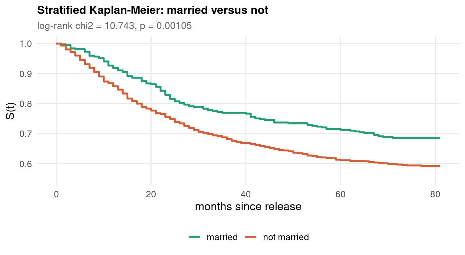
Stratified Curves

Code
data("recid", package = "wooldridge")
recid <- transform(recid, fail = 1 - cens)

km2 <- survfit(Surv(durat, fail) ~ married, data = recid)

strata <- rep(names(km2$strata), km2$strata)
curve  <- data.frame(t = km2$time, S = km2$surv,
                     grp = ifelse(strata == "married=1", "married", "not married"))
curve  <- rbind(data.frame(t = c(0, 0), S = c(1, 1),
                           grp = c("married", "not married")), curve)

ggplot(curve) +
  aes(x = t, y = S, colour = grp) +
  geom_step(linewidth = 1.1) +
  scale_colour_manual(values = c("married" = "#1D9E75",
                                 "not married" = "#D85A30")) +
  coord_cartesian(xlim = c(0, 81), ylim = c(0.55, 1)) +
  scale_x_continuous(breaks = seq(0, 80, 20)) +
  scale_y_continuous(breaks = seq(0.6, 1, 0.1)) +
  labs(x = "months since release", y = "S(t)", colour = NULL,
       title = "Stratified Kaplan-Meier: married versus not",
       subtitle = "log-rank chi2 = 10.743, p = 0.00105")
Code
import numpy as np
import matplotlib.pyplot as plt
import wooldridge as woo
from lifelines import KaplanMeierFitter

rc = woo.data('recid').assign(fail=lambda d: 1 - d['cens'])

fig, ax = plt.subplots(figsize=(8, 4.4))
for val, lab, col in [(1, "married", "#1D9E75"), (0, "not married", "#D85A30")]:
    g = rc[rc['married'] == val]
    km = KaplanMeierFitter().fit(g['durat'], g['fail'])
    ax.step(km.survival_function_.index.values,
            km.survival_function_.iloc[:, 0].values,
            where="post", color=col, lw=1.8, label=lab)
ax.text(0.03, 0.10, "log-rank chi2 = 10.743, p = 0.00105",
        transform=ax.transAxes, fontsize=10, color="#185FA5")
axopts = ax.set(xlim=(0, 81), ylim=(0.55, 1.0), xticks=range(0, 81, 20),
                yticks=np.arange(0.6, 1.01, 0.1),
                xlabel="months since release", ylabel="S(t)",
                title="Stratified Kaplan-Meier: married versus not")
ax.legend(frameon=False, loc="lower left")
plt.show()
Code
quietly frause recid, clear
gen fail = 1 - cens
quietly stset durat, failure(fail == 1)

sts graph, by(married)                                                        ///
    plot1opts(lcolor("216 90 48")  lwidth(medthick))                          ///
    plot2opts(lcolor("29 158 117") lwidth(medthick))                          ///
    xscale(range(0 81)) xlabel(0(20)80)                                       ///
    yscale(range(0.55 1)) ylabel(0.6(0.1)1)                                   ///
    xtitle("months since release") ytitle("S(t)")                             ///
    title("Stratified Kaplan-Meier: married versus not", size(medium))        ///
    subtitle("log-rank chi2 = 10.743, p = 0.00105", size(small))              ///
    legend(order(1 "not married" 2 "married") rows(1) position(6) ring(1) region(lstyle(none)))   ///
    graphregion(color(white)) plotregion(color(white)) xsize(8) ysize(4.4)
graph export "../plots/dsc-p2-strat.png", replace width(1600)
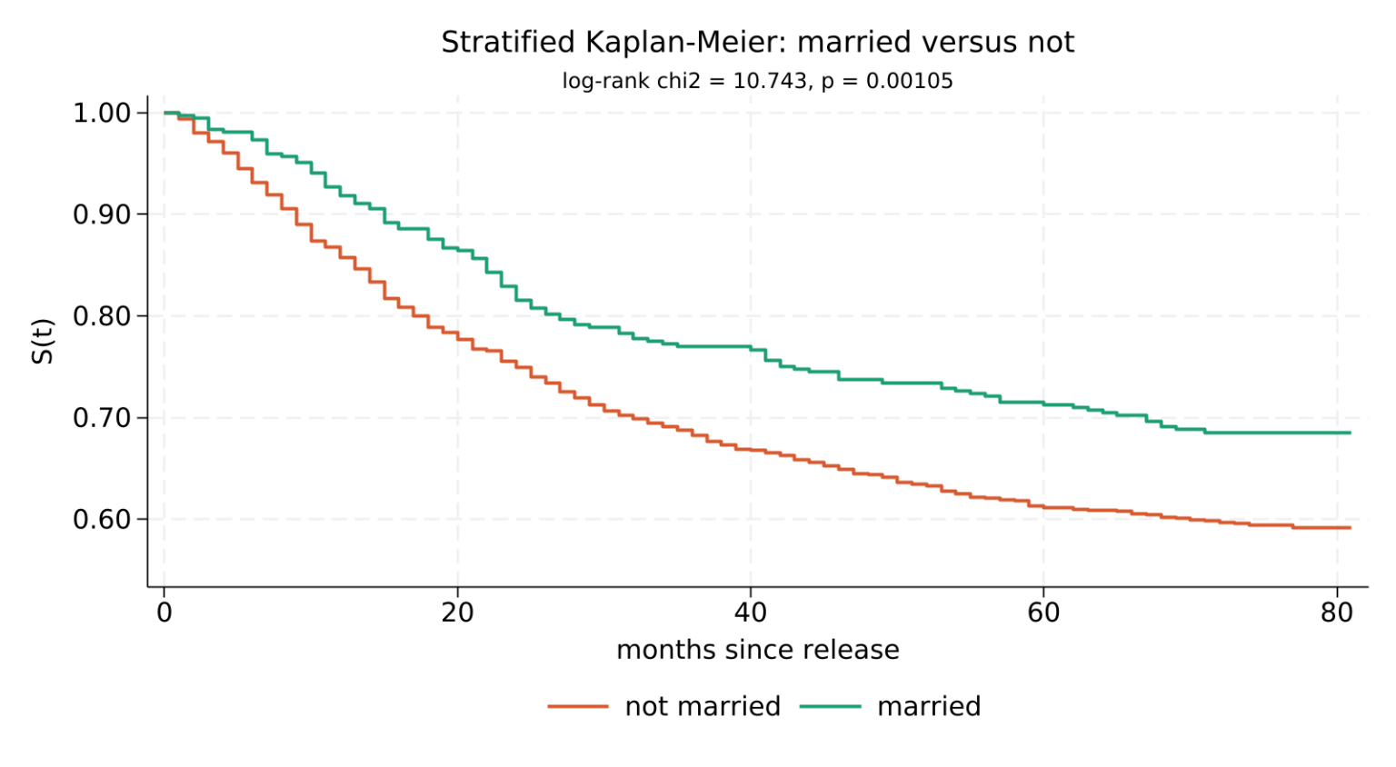
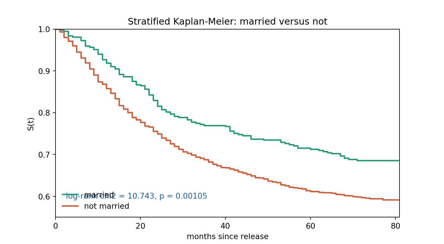
Married men survive better at every horizon: \(\hat S(36) = 0.7696\) against \(0.6822\), and \(\hat S(80) = 0.6854\) against \(0.5916\). The curves separate early and never cross — the visual signature of proportional hazards, and a reason to expect Part 3’s Cox model to fit this data.

Stop here when the comparison is one binary variable, the curves do not cross, and nobody is claiming causality. A stratified Kaplan–Meier plus a log-rank test is a complete, assumption-light answer, and it is more honest than a regression table implying control you do not have.

Go on to Part 3 when you need more than one covariate, a continuous covariate, an effect size rather than a \(p\)-value, or covariates that change during the spell. Stratification delivers none of those: splitting on age, race, marriage and priors at once leaves cells holding a handful of men and no curve worth drawing.

Part 3 — Cox and Proportional Hazards

Partial likelihood, ties, and testing the assumption

The Proportional-Hazards Idea

Part 2 could describe survival but not explain it. The obvious next step — write down a full parametric hazard — forces a commitment about the shape of \(h(t)\) that no economic theory supplies. Cox’s idea is to avoid the commitment entirely:

\[h(t \mid \mathbf{x}) = h_0(t)\,\exp(\mathbf{x}'\boldsymbol{\beta})\]

The hazard factors into a baseline \(h_0(t)\), shared by everyone and left completely unspecified, and a multiplier \(\exp(\mathbf{x}'\boldsymbol{\beta})\) that does not depend on time.

Time affects everyone the same way. Covariates shift the whole hazard up or down by a constant factor. That is the entire content of “proportional hazards”.

Take two men with covariates \(\mathbf{x}_a\) and \(\mathbf{x}_b\). Their hazard ratio is

\[\frac{h(t \mid \mathbf{x}_a)}{h(t \mid \mathbf{x}_b)} = \frac{h_0(t)\exp(\mathbf{x}_a'\boldsymbol{\beta})}{h_0(t)\exp(\mathbf{x}_b'\boldsymbol{\beta})} = \exp\!\big[(\mathbf{x}_a - \mathbf{x}_b)'\boldsymbol{\beta}\big]\]

\(h_0(t)\) cancels. The ratio is constant in \(t\) — the same at month 3 and at month 60.

Equivalently, on the log cumulative-hazard scale the two curves are parallel:

\[\log H(t \mid \mathbf{x}) = \log H_0(t) + \mathbf{x}'\boldsymbol{\beta}\]

which is exactly what the \(\log(-\log \hat S)\) diagnostic plot looks for, and it is why the married and unmarried curves of Part 2 were worth a second look.

Proportionality is restrictive, and it is testable. A treatment that helps early and stops helping later violates it. So does anything whose effect builds over time — training that pays off only once completed, a benefit rule that binds at a fixed date. Both are ordinary in labour economics.

Two slides from now the assumption gets tested rather than assumed. What makes the Cox model worth its restriction is that everything else about \(h_0\) goes unspecified: no distributional family, no shape, no duration-dependence commitment, and — the next slide — no need to estimate \(h_0\) at all.

Partial Likelihood

Order the event times \(t_{(1)} < \cdots < t_{(k)}\) and ask a modest question at each one: given that exactly one failure happens now, which member of the risk set is it?

For the individual \(i\) who actually failed at \(t_{(j)}\), the probability of that outcome under the model is the ratio of their hazard to the total hazard in the risk set:

\[L_j(\boldsymbol{\beta}) = \frac{h_0(t_{(j)})\exp(\mathbf{x}_i'\boldsymbol{\beta})} {\sum_{\ell \in R(t_{(j)})} h_0(t_{(j)})\exp(\mathbf{x}_\ell'\boldsymbol{\beta})} = \frac{\exp(\mathbf{x}_i'\boldsymbol{\beta})} {\sum_{\ell \in R(t_{(j)})} \exp(\mathbf{x}_\ell'\boldsymbol{\beta})}\]

\(h_0(t_{(j)})\) cancels from numerator and denominator. Multiply across event times:

\[\boxed{\; L_P(\boldsymbol{\beta}) = \prod_{j=1}^{k} \frac{\exp(\mathbf{x}_{(j)}'\boldsymbol{\beta})} {\sum_{\ell \in R(t_{(j)})} \exp(\mathbf{x}_\ell'\boldsymbol{\beta})} \;}\]

The infinite-dimensional nuisance parameter \(h_0(\cdot)\) has vanished, and what remains is a function of \(\boldsymbol{\beta}\) alone. It has the algebraic form of a conditional logit over the risk set — which is why the optimisation is easy and globally well behaved.

\(L_P\) is not a likelihood: it is a product of conditional probabilities, and it does not integrate to one over any sample space. Yet it behaves like one — Cox (1975) showed the score has mean zero and the usual sandwich collapses, so

\[\hat{\boldsymbol{\beta}} \overset{a}{\sim} \mathcal{N}\!\left(\boldsymbol{\beta}, \;\mathcal{I}(\hat{\boldsymbol{\beta}})^{-1}\right)\]

with \(\mathcal{I}\) the usual observed information from \(-\partial^2 \log L_P\).

The prices paid:

  • Only the ranks of the event times matter. Doubling every duration changes nothing. Great for robustness, useless if you want to predict a duration.
  • Some efficiency is lost relative to a correctly specified parametric model. How much is an empirical question, and Part 4 measures it on this data: essentially nothing.
  • \(h_0\) is not estimated during fitting. It can be recovered afterwards (last slide of this part), but as a by-product rather than a parameter.
  • Censored spells contribute only through the risk set. They appear in denominators and never in a numerator.

The derivation above assumed one failure per time point. recid measures time in whole months, so it has 552 events spread over just 74 distinct times — an average of \(7.5\) events per event time and up to \(23\) at once. Ties are not a corner case here; they are the norm.

Three treatments, in increasing order of correctness and cost:

Breslow — pretend the tied events all faced the same denominator:

\[L_j = \frac{\exp\big(\sum_{i \in D_j} \mathbf{x}_i'\boldsymbol{\beta}\big)} {\left[\sum_{\ell \in R_j} \exp(\mathbf{x}_\ell'\boldsymbol{\beta})\right]^{d_j}}\]

Fast, and biased toward zero when ties are heavy.

Efron — shrink the denominator progressively, as the tied failures are notionally removed one by one. Almost as fast as Breslow, far more accurate, and the right default.

Exact — sum over all \(d_j!\) orderings of the tied events. Correct, and expensive; note that its log-likelihood is a different object and cannot be compared with the other two.

Stata’s stcox defaults to Breslow. R’s coxph and lifelines default to Efron. Run the same model in two packages, get two answers, and spend an afternoon looking for a data bug that is not there. On the next slide the Stata tab writes , efron explicitly, and the three tabs then agree to six decimals.

Cox on recid

The Wooldridge Chapter 22 specification: does the prison work programme reduce the hazard of returning, holding criminal history and demographics fixed?

Code
library(survival)
data("recid", package = "wooldridge")
recid <- transform(recid, fail = 1 - cens)

# ties = "efron" is the default in R; it is written out here because
# Stata's default is Breslow and the two do not agree.
cx <- coxph(Surv(durat, fail) ~ workprg + priors + tserved + felon + alcohol +
              drugs + black + married + educ + age,
            data = recid, ties = "efron")
summary(cx)
Call:
coxph(formula = Surv(durat, fail) ~ workprg + priors + tserved + 
    felon + alcohol + drugs + black + married + educ + age, data = recid, 
    ties = "efron")

  n= 1445, number of events= 552 

              coef  exp(coef)   se(coef)      z Pr(>|z|)    
workprg  0.0844047  1.0880692  0.0908109  0.929  0.35265    
priors   0.0880165  1.0920062  0.0134634  6.537 6.26e-11 ***
tserved  0.0130652  1.0131509  0.0016827  7.765 8.20e-15 ***
felon   -0.2839037  0.7528391  0.1061160 -2.675  0.00746 ** 
alcohol  0.4329985  1.5418739  0.1057236  4.096 4.21e-05 ***
drugs    0.2776044  1.3199639  0.0978660  2.837  0.00456 ** 
black    0.4350647  1.5450631  0.0883757  4.923 8.53e-07 ***
married -0.1551368  0.8562981  0.1092094 -1.421  0.15545    
educ    -0.0213612  0.9788653  0.0194458 -1.099  0.27198    
age     -0.0036055  0.9964010  0.0005228 -6.896 5.34e-12 ***
---
Signif. codes:  0 '***' 0.001 '**' 0.01 '*' 0.05 '.' 0.1 ' ' 1

        exp(coef) exp(-coef) lower .95 upper .95
workprg    1.0881     0.9191    0.9107    1.3000
priors     1.0920     0.9157    1.0636    1.1212
tserved    1.0132     0.9870    1.0098    1.0165
felon      0.7528     1.3283    0.6115    0.9269
alcohol    1.5419     0.6486    1.2533    1.8969
drugs      1.3200     0.7576    1.0896    1.5991
black      1.5451     0.6472    1.2993    1.8373
married    0.8563     1.1678    0.6913    1.0607
educ       0.9789     1.0216    0.9423    1.0169
age        0.9964     1.0036    0.9954    0.9974

Concordance= 0.661  (se = 0.012 )
Likelihood ratio test= 157.4  on 10 df,   p=<2e-16
Wald test            = 168.2  on 10 df,   p=<2e-16
Score (logrank) test = 170.9  on 10 df,   p=<2e-16
Code
import wooldridge as woo
from lifelines import CoxPHFitter

rc = woo.data('recid').assign(fail=lambda d: 1 - d['cens'])
X = ['workprg', 'priors', 'tserved', 'felon', 'alcohol',
     'drugs', 'black', 'married', 'educ', 'age']

# lifelines uses Efron for ties, like R
cp = CoxPHFitter().fit(rc[X + ['durat', 'fail']], 'durat', 'fail')

out = cp.summary[['coef', 'exp(coef)', 'se(coef)', 'z', 'p',
                  'exp(coef) lower 95%', 'exp(coef) upper 95%']].round(5)
txt = (out.to_string() +
       "\n\npartial log-likelihood = %.4f   n = %d   events = %d"
       % (cp.log_likelihood_, cp._n_examples, int(rc['fail'].sum())))

import sys
nw = sys.stdout.write(txt + "\n")
              coef  exp(coef)  se(coef)        z        p  exp(coef) lower 95%  exp(coef) upper 95%
covariate                                                                                          
workprg    0.08440    1.08807   0.09081  0.92946  0.35265              0.91066              1.30003
priors     0.08802    1.09201   0.01346  6.53745  0.00000              1.06357              1.12121
tserved    0.01307    1.01315   0.00168  7.76452  0.00000              1.00982              1.01650
felon     -0.28390    0.75284   0.10612 -2.67541  0.00746              0.61147              0.92689
alcohol    0.43300    1.54187   0.10572  4.09557  0.00004              1.25330              1.89688
drugs      0.27760    1.31996   0.09787  2.83658  0.00456              1.08958              1.59906
black      0.43506    1.54506   0.08838  4.92290  0.00000              1.29933              1.83726
married   -0.15514    0.85630   0.10921 -1.42054  0.15545              0.69130              1.06068
educ      -0.02136    0.97887   0.01945 -1.09850  0.27198              0.94226              1.01689
age       -0.00361    0.99640   0.00052 -6.89623  0.00000              0.99538              0.99742

partial log-likelihood = -3813.0785   n = 1445   events = 552
Code
sys.stdout.flush()
Code
quietly frause recid, clear
gen fail = 1 - cens
quietly stset durat, failure(fail == 1)
* efron is NOT Stata's default - stcox uses Breslow unless told otherwise
stcox workprg priors tserved felon alcohol drugs black married educ age, efron nolog
        Failure _d: fail==1
  Analysis time _t: durat

Cox regression with Efron method for ties

No. of subjects =  1,445                                Number of obs =  1,445
No. of failures =    552
Time at risk    = 80,013
                                                        LR chi2(10)   = 157.39
Log likelihood = -3813.0785                             Prob > chi2   = 0.0000

------------------------------------------------------------------------------
          _t | Haz. ratio   Std. err.      z    P>|z|     [95% conf. interval]
-------------+----------------------------------------------------------------
     workprg |   1.088069   .0988086     0.93   0.353     .9106638    1.300035
      priors |   1.092006   .0147022     6.54   0.000     1.063567    1.121205
     tserved |   1.013151   .0017048     7.76   0.000     1.009815    1.016498
       felon |   .7528391   .0798883    -2.68   0.007     .6114712    .9268902
     alcohol |   1.541874   .1630125     4.10   0.000     1.253305    1.896885
       drugs |   1.319964   .1291796     2.84   0.005     1.089578    1.599064
       black |   1.545063    .136546     4.92   0.000     1.299334    1.837265
     married |   .8562981   .0935158    -1.42   0.155     .6912987     1.06068
        educ |   .9788653   .0190348    -1.10   0.272     .9422598    1.016893
         age |    .996401   .0005209    -6.90   0.000     .9953805    .9974226
------------------------------------------------------------------------------
    ties   priors  tserved    black     logPL
   efron 0.088017 0.013065 0.435065 -3813.079
 breslow 0.087592 0.012950 0.432593 -3816.380
   exact 0.088947 0.013206 0.437576 -2973.141

With \(7.5\) events per event time, Breslow attenuates every coefficient toward zero — black moves from \(0.4351\) to \(0.4326\), priors from \(0.0880\) to \(0.0876\). Small here, but the bias grows with the number of ties, and it is entirely avoidable.

The exact log-likelihood is a different object (a marginal rather than a partial likelihood) and must not be compared with the other two rows; its coefficients are the ones worth reading, and Efron tracks them closely.

Parity. All three report a partial log-likelihood of \(-3813.0785\) and identical coefficients — workprg \(0.084405\) (HR \(1.0881\)), priors \(0.088017\) (HR \(1.0920\)), tserved \(0.013065\) (HR \(1.0131\)), black \(0.435065\) (HR \(1.5451\)). Stata reaches them only because efron was written out.

Reading Hazard Ratios

Covariate HR Reading
workprg \(1.0881\) work-programme men have an 8.8% higher monthly hazard — wrong sign for the policy, and \(p = 0.35\), so indistinguishable from no effect
priors \(1.0920\) each prior conviction raises the hazard 9.2%; ten priors multiply it by \(1.092^{10} = 2.4\)
tserved \(1.0131\) each month served raises the hazard 1.3%; a year served raises it \(1.0131^{12} = 1.17\)
alcohol \(1.5419\) a history of alcohol abuse raises the hazard 54%
black \(1.5451\) a 55% higher hazard, conditional on this covariate set
age \(0.9964\) age is in months; per year the factor is \(0.9964^{12} = 0.958\), a 4.2% lower hazard

The workprg result is the point of the exercise, and it is a null. The programme is not randomly assigned; men are selected into it, and Wooldridge reaches the same conclusion from the AFT regression in Part 4.

1. A hazard ratio is not a duration ratio. \(\mathrm{HR} = 1.5\) does not mean spells are one-third shorter. The mapping runs through the whole baseline, and for a Weibull with shape \(p\) it is

\[\frac{\mathbb{E}[T \mid \mathbf{x}_a]}{\mathbb{E}[T \mid \mathbf{x}_b]} = \mathrm{HR}^{-1/p}\]

With \(p = 0.805864\) from Part 4, an HR of \(1.5451\) for black implies a median duration ratio of \(1.5451^{-1/0.805864} = 0.583\) — a 42% shorter time to re-arrest, not 55%. Report the transformed quantity when the audience thinks in durations.

2. It is an average over survivors, not an individual effect. By month 40 the men still at risk are a selected group. If unobserved heterogeneity is present, the estimated HR is attenuated toward 1 as \(t\) grows even when the individual ratio is constant — Part 5, at length.

3. “No effect on duration” is not “no effect”. The hazard is a rate. A covariate can leave the hazard alone while changing which exit occurs — the competing-risks distinction of Part 6.

Economists often want \(\partial \mathbb{E}[T]/\partial x\) rather than a ratio. It exists, but it is not a property of \(\boldsymbol{\beta}\) alone:

\[\mathbb{E}[T \mid \mathbf{x}] = \int_0^\infty S(u \mid \mathbf{x})\,du = \int_0^\infty \exp\!\big[-H_0(u)e^{\mathbf{x}'\boldsymbol{\beta}}\big] du\]

The integral needs \(H_0\), which the Cox model deliberately did not estimate, and it needs \(H_0\) beyond the last observed event time, where the data say nothing. That extrapolation is exactly what a parametric model supplies, and it is the strongest argument for Part 4.

Testing Proportional Hazards

For each event, the Schoenfeld residual is the failing individual’s covariate minus the risk-set average, weighted by the fitted probabilities:

\[\mathbf{r}_j = \mathbf{x}_{(j)} - \bar{\mathbf{x}}(\hat{\boldsymbol{\beta}}, t_{(j)}), \qquad \bar{\mathbf{x}} = \frac{\sum_{\ell \in R_j} \mathbf{x}_\ell e^{\mathbf{x}_\ell'\hat{\boldsymbol{\beta}}}} {\sum_{\ell \in R_j} e^{\mathbf{x}_\ell'\hat{\boldsymbol{\beta}}}}\]

These are the individual terms of the score, so under a correct model they have mean zero and no pattern in time.

Grambsch & Therneau (1994) scale them so that

\[\mathbb{E}\big[\mathbf{r}^{*}_j\big] \approx \boldsymbol{\beta}(t_{(j)}) - \boldsymbol{\beta}\]

Then testing proportional hazards becomes testing whether the scaled residuals have a slope against time:

\[H_0: \boldsymbol{\beta}(t) = \boldsymbol{\beta} \quad\text{for all } t \qquad\Longleftrightarrow\qquad H_0: \text{zero correlation between } \mathbf{r}^{*} \text{ and } g(t)\]

which is a \(\chi^2_1\) test per covariate and a \(\chi^2_p\) global test.

The test needs a time scale, and the answer depends on it — a genuine choice, not a nuisance.

\(g(t)\) Name Emphasises
\(t\) identity late times, where few remain at risk
\(\mathrm{rank}(t)\) rank all event times equally
\(1 - \hat S(t)\) Kaplan–Meier event-time density; the usual default
\(\log t\) log early times

On recid the global statistic runs from \(13.85\) (identity) to \(16.52\) (log) — the same data, the same model, four defensible transforms, and no rejection under any of them. Report which one you used.

R’s cox.zph defaults to the KM transform; Stata’s estat phtest defaults to identity. The code slide writes , km on the Stata call so all three tabs test the same hypothesis on the same scale.

Under proportional hazards,

\[\log\{-\log S(t \mid \mathbf{x})\} = \log H_0(t) + \mathbf{x}'\boldsymbol{\beta}\]

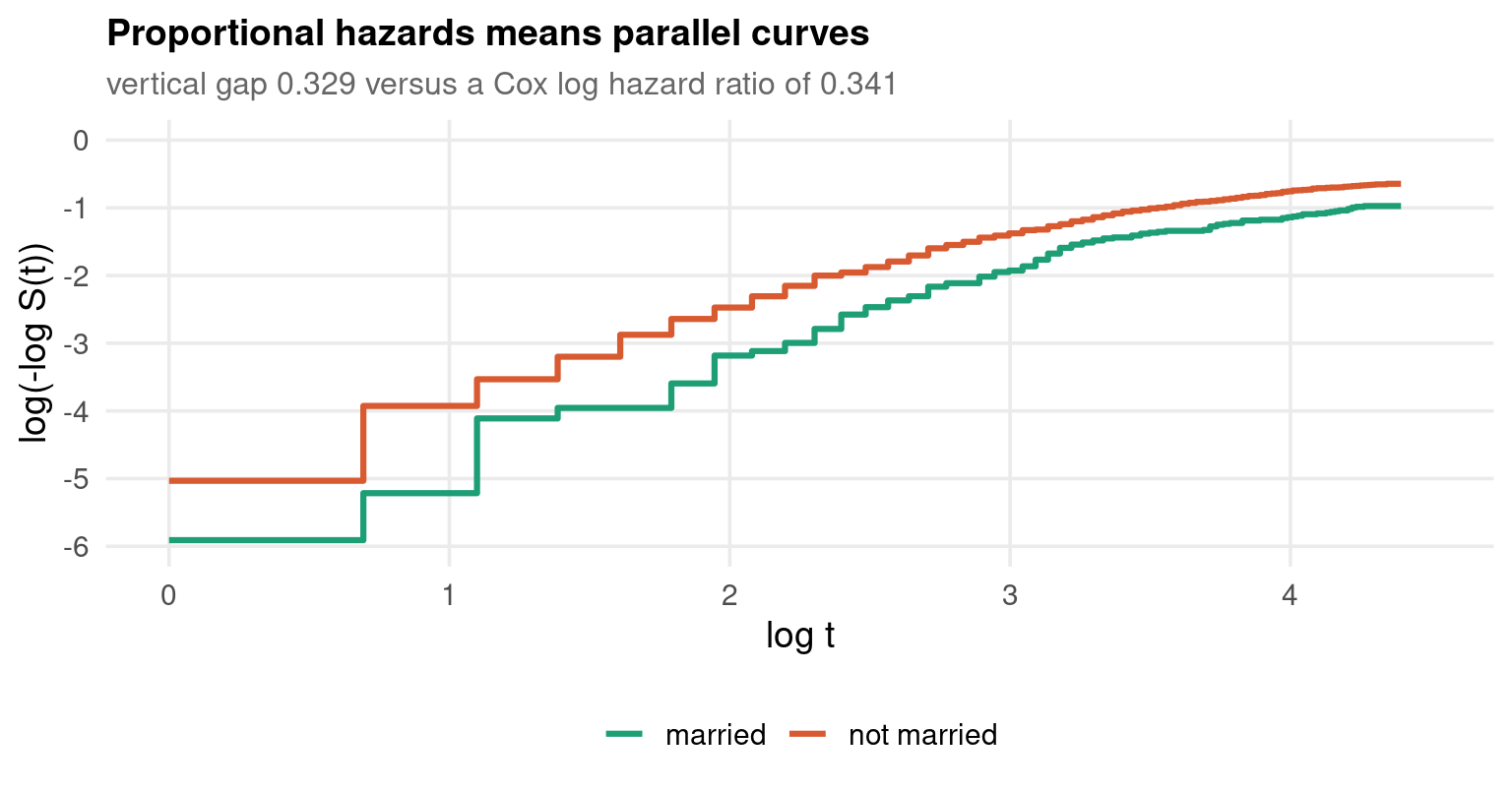
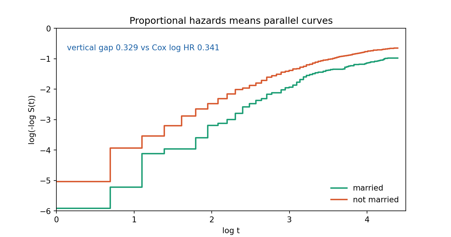
so plotting \(\log(-\log \hat S)\) against \(\log t\) for two groups should give two parallel curves, vertically separated by the log hazard ratio.

Converging, diverging or crossing curves are proportional-hazards failures, and the plot says how it fails — which the \(\chi^2\) never does. It is limited to categorical covariates with reasonable cell sizes, so it complements the test rather than replacing it.

PH Diagnostics — Code

Code
data("recid", package = "wooldridge")
recid <- transform(recid, fail = 1 - cens)
cx <- coxph(Surv(durat, fail) ~ workprg + priors + tserved + felon + alcohol +
              drugs + black + married + educ + age,
            data = recid, ties = "efron")

# transform = "km" is R's default; named here so all three tabs match
z <- cox.zph(cx, transform = "km")
print(z)
           chisq df     p
workprg 1.45e+00  1 0.228
priors  3.32e+00  1 0.068
tserved 2.48e+00  1 0.115
felon   1.78e-01  1 0.673
alcohol 2.31e+00  1 0.129
drugs   4.20e-02  1 0.838
black   5.57e-01  1 0.455
married 3.59e+00  1 0.058
educ    6.38e-01  1 0.424
age     3.31e-05  1 0.995
GLOBAL  1.59e+01 10 0.103
Code
import wooldridge as woo
from lifelines import CoxPHFitter
from lifelines.statistics import proportional_hazard_test

rc = woo.data('recid').assign(fail=lambda d: 1 - d['cens'])
X = ['workprg', 'priors', 'tserved', 'felon', 'alcohol',
     'drugs', 'black', 'married', 'educ', 'age']
df = rc[X + ['durat', 'fail']]
cp = CoxPHFitter().fit(df, 'durat', 'fail')

ph = proportional_hazard_test(cp, df, time_transform='km')
tab = ph.summary[['test_statistic', 'p']].round(5)
txt = (tab.to_string() +
       "\n\nlifelines reports no global test; the sum of the per-covariate\n"
       "statistics is %.2f on 10 df." % tab['test_statistic'].sum())

import sys
nw = sys.stdout.write(txt + "\n")
         test_statistic        p
age             0.70029  0.40268
alcohol         1.93358  0.16437
black           0.73376  0.39167
drugs           0.06262  0.80240
educ            1.91829  0.16605
felon           0.01730  0.89536
married         2.17974  0.13984
priors          3.60714  0.05753
tserved         2.95090  0.08583
workprg         1.38635  0.23902

lifelines reports no global test; the sum of the per-covariate
statistics is 15.49 on 10 df.
Code
sys.stdout.flush()
Code
quietly frause recid, clear
gen fail = 1 - cens
quietly stset durat, failure(fail == 1)
quietly stcox workprg priors tserved felon alcohol drugs black married educ age, efron
* km is NOT the default - estat phtest uses analysis time unless told otherwise
estat phtest, km detail
Test of proportional-hazards assumption

Time function: 1 - Kaplan–Meier estimate
--------------------------------------------------------
             |        rho     chi2       df    Prob>chi2
-------------+------------------------------------------
     workprg |    0.04994     1.39        1       0.2384
      priors |   -0.08817     3.49        1       0.0618
     tserved |   -0.08999     3.07        1       0.0800
       felon |    0.00480     0.01        1       0.9142
     alcohol |   -0.05935     1.92        1       0.1659
       drugs |    0.00984     0.05        1       0.8178
       black |    0.03643     0.71        1       0.3981
     married |    0.06155     2.15        1       0.1427
        educ |   -0.06300     1.95        1       0.1627
         age |    0.03064     0.68        1       0.4091
-------------+------------------------------------------
 Global test |               15.84       10       0.1043
--------------------------------------------------------
Code
data("recid", package = "wooldridge")
recid <- transform(recid, fail = 1 - cens)
km2 <- survfit(Surv(durat, fail) ~ married, data = recid)

strata <- rep(names(km2$strata), km2$strata)
ll <- data.frame(t = km2$time, S = km2$surv,
                 grp = ifelse(strata == "married=1", "married", "not married"))
ll <- subset(ll, S > 0 & S < 1)
ll <- transform(ll, x = log(t), y = log(-log(S)))

ggplot(ll) +
  aes(x = x, y = y, colour = grp) +
  geom_step(linewidth = 1.1) +
  scale_colour_manual(values = c("married" = "#1D9E75",
                                 "not married" = "#D85A30")) +
  coord_cartesian(xlim = c(0, 4.5), ylim = c(-6, 0)) +
  scale_x_continuous(breaks = seq(0, 4, 1)) +
  scale_y_continuous(breaks = seq(-6, 0, 1)) +
  labs(x = "log t", y = "log(-log S(t))", colour = NULL,
       title = "Proportional hazards means parallel curves",
       subtitle = "vertical gap 0.329 versus a Cox log hazard ratio of 0.341")
Code
import numpy as np
import matplotlib.pyplot as plt
import wooldridge as woo
from lifelines import KaplanMeierFitter

rc = woo.data('recid').assign(fail=lambda d: 1 - d['cens'])

fig, ax = plt.subplots(figsize=(8, 4.2))
for val, lab, col in [(1, "married", "#1D9E75"), (0, "not married", "#D85A30")]:
    g = rc[rc['married'] == val]
    km = KaplanMeierFitter().fit(g['durat'], g['fail'])
    t = km.survival_function_.index.values
    S = km.survival_function_.iloc[:, 0].values
    ok = (S > 0) & (S < 1) & (t > 0)
    ax.step(np.log(t[ok]), np.log(-np.log(S[ok])), where="post",
            color=col, lw=1.8, label=lab)
ax.text(0.03, 0.88, "vertical gap 0.329 vs Cox log HR 0.341",
        transform=ax.transAxes, fontsize=10, color="#185FA5")
axopts = ax.set(xlim=(0, 4.5), ylim=(-6, 0), xticks=range(0, 5),
                yticks=range(-6, 1), xlabel="log t", ylabel="log(-log S(t))",
                title="Proportional hazards means parallel curves")
ax.legend(frameon=False, loc="lower right")
plt.show()
Code
quietly frause recid, clear
gen fail = 1 - cens
quietly stset durat, failure(fail == 1)

* stphplot would plot MINUS log(-log S), the mirror image of the R and Python
* tabs, so the transform is built by hand instead
quietly sts gen S = s, by(married)
quietly gen y = ln(-ln(S)) if S > 0 & S < 1
quietly gen x = ln(durat)

twoway (line y x if married == 0, sort connect(stairstep)                     ///
            lcolor("216 90 48")  lwidth(medthick))                            ///
       (line y x if married == 1, sort connect(stairstep)                     ///
            lcolor("29 158 117") lwidth(medthick)),                           ///
    xscale(range(0 4.5)) xlabel(0(1)4)                                        ///
    yscale(range(-6 0)) ylabel(-6(1)0)                                        ///
    xtitle("log t") ytitle("log(-log S(t))")                                  ///
    title("Proportional hazards means parallel curves", size(medium))         ///
    subtitle("vertical gap 0.329 versus a Cox log hazard ratio of 0.341", size(small)) ///
    legend(order(1 "not married" 2 "married") rows(1) position(6) ring(1) region(lstyle(none)))   ///
    graphregion(color(white)) plotregion(color(white)) xsize(8) ysize(4.2)
graph export "../plots/dsc-p3-loglog.png", replace width(1600)
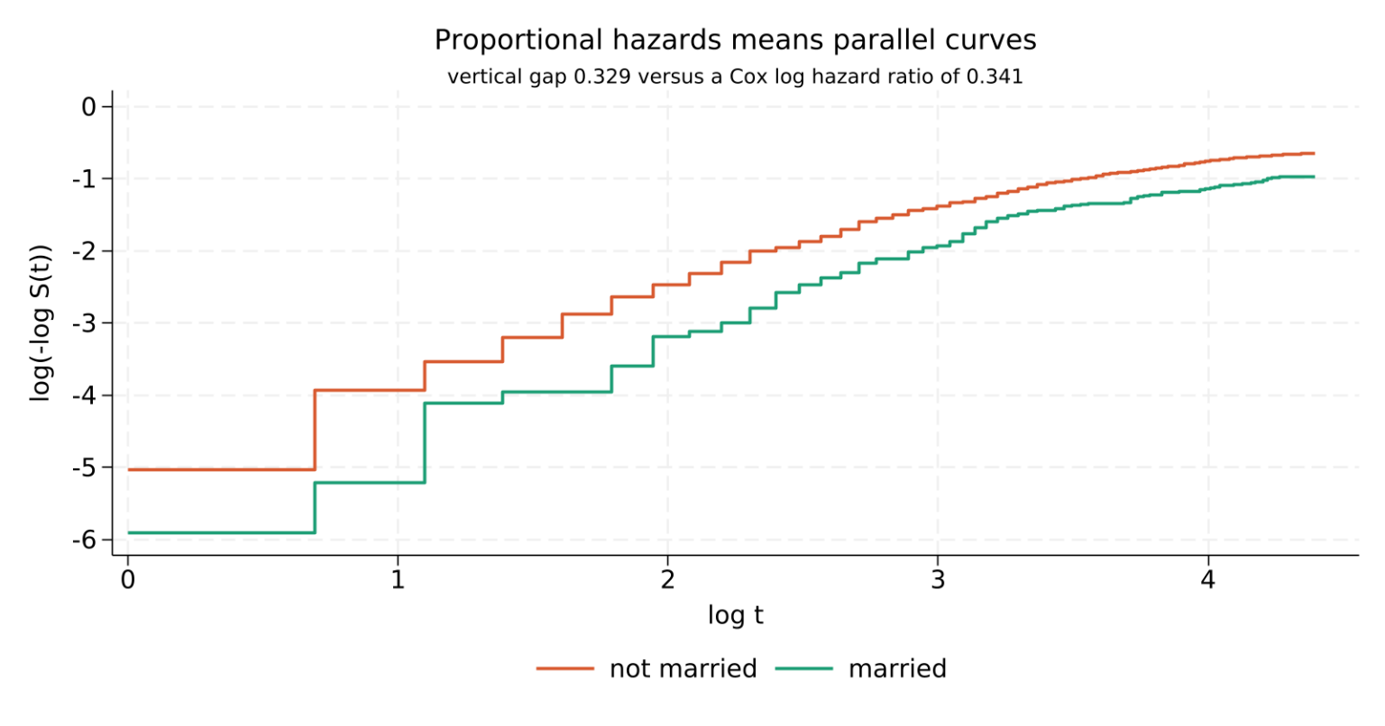
The verdict is the same everywhere: proportional hazards is not rejected. The global statistic is \(15.88\) (\(p = 0.103\)) in R and \(15.84\) (\(p = 0.104\)) in Stata; lifelines reports no global test, and its per-covariate statistics sum to \(15.49\). Nothing is significant at 5%; priors is the closest, at \(p \approx 0.06\).

When Proportional Hazards Fails

1. Stratify. Let the offending covariate have its own baseline:

\[h(t \mid \mathbf{x}, s) = h_{0s}(t)\,\exp(\mathbf{x}'\boldsymbol{\beta})\]

The partial likelihood becomes a product over strata. Cheap, and requires nothing new. The cost is that the stratifying variable loses its coefficient — you control for it but can no longer report its effect.

2. Interact with time. Let the coefficient move:

\[h(t \mid \mathbf{x}) = h_0(t)\exp\big[\beta_1 x + \beta_2\, x \cdot g(t)\big]\]

Then \(\beta_2\) is the violation, estimated and testable. It keeps the covariate in the model and describes how its effect evolves. The next slide does exactly this.

3. Split the time axis. Fit separate models on \([0, \tau)\) and \([\tau, \infty)\) when there is a substantive breakpoint — benefit exhaustion, contract expiry, a policy date. Honest, interpretable, and it needs a reason for \(\tau\) that is not the data.

4. Change model. An accelerated-failure-time specification (Part 4) makes a different assumption, not a weaker one, but a covariate that fails PH may satisfy AFT. Log-logistic and log-normal are AFT-only families, and they permit non-monotone hazards.

Situation Response
Nuisance control, effect not of interest stratify
The effect of interest changes over time interact with time — and report the interaction, it is a finding
A known institutional date split the axis at that date
Many covariates fail at once suspect misspecification or frailty, not PH — go to Part 5
You need to extrapolate beyond the data parametric AFT, Part 4

Do not stratify on a continuous covariate by binning it. That throws away the information you have and creates an arbitrary grid; interact it with time instead.

A significant Schoenfeld test is a finding about the world, not a defect to be patched. “The training effect is strong in the first six months and gone by month twelve” is a more useful sentence than a single averaged hazard ratio, and it is exactly what the time interaction estimates.

The failure mode to avoid is the opposite: fitting a Cox model, never testing, and reporting one hazard ratio as if it held throughout. On this data it happens to hold; that had to be checked, not assumed.

Time-Varying Covariates

Nothing in the partial likelihood requires \(\mathbf{x}\) to be fixed. Only the risk-set sum matters, so each unit may be represented by several rows, each covering an interval over which its covariates are constant:

\[L_P(\boldsymbol{\beta}) = \prod_{j} \frac{\exp\big(\mathbf{x}_{(j)}(t_{(j)})'\boldsymbol{\beta}\big)} {\sum_{\ell \in R(t_{(j)})} \exp\big(\mathbf{x}_\ell(t_{(j)})'\boldsymbol{\beta}\big)}\]

Everyone contributes the covariate values they held at that moment. Written as data, one man becomes several rows:

id start stop event benefit
7 0 26 0 1
7 26 41 1 0
  • R — Surv(start, stop, event), built by survSplit() or tmerge()
  • Stata — stset ..., id() then stsplit; or tvc() for the interaction case
  • Python — CoxTimeVaryingFitter on long-format data

Only genuinely external covariates may vary. A covariate that is itself caused by the process — health during an illness, search effort during a spell — makes the estimand meaningless: you are conditioning on an outcome. Calendar time, benefit rules and policy dates are safe; anything the unit chooses is not.

Code
data("recid", package = "wooldridge")
recid <- transform(recid, fail = 1 - cens)

# Does the effect of time served drift over the spell?
# tt() builds the interaction x * log(t) at each risk set.
ctv <- coxph(Surv(durat, fail) ~ workprg + priors + tserved + felon + alcohol +
               drugs + black + married + educ + age + tt(tserved),
             data = recid, ties = "efron",
             tt = function(x, t, ...) x * log(t))

print(round(summary(ctv)$coefficients[c("tserved", "tt(tserved)"), ], 6))

cx <- coxph(Surv(durat, fail) ~ workprg + priors + tserved + felon + alcohol +
              drugs + black + married + educ + age, data = recid, ties = "efron")
cat("\nlogPL constant effect =", round(cx$loglik[2], 4),
    "\nlogPL time-varying    =", round(ctv$loglik[2], 4),
    "\nLR statistic          =", round(2 * (ctv$loglik[2] - cx$loglik[2]), 4), "\n")
                 coef exp(coef) se(coef)         z Pr(>|z|)
tserved      0.016839  1.016982 0.004016  4.192763 0.000028
tt(tserved) -0.001476  0.998525 0.001470 -1.004303 0.315232

logPL constant effect = -3813.079 
logPL time-varying    = -3812.585 
LR statistic          = 0.9872 
Code
import numpy as np
import pandas as pd
import wooldridge as woo
from lifelines import CoxTimeVaryingFitter, CoxPHFitter

rc = woo.data('recid').assign(fail=lambda d: 1 - d['cens'])
rc = rc.assign(id=np.arange(len(rc)))
X = ['workprg', 'priors', 'tserved', 'felon', 'alcohol',
     'drugs', 'black', 'married', 'educ', 'age']

# expand to one row per month at risk, then build tserved * log(t) per row
rows = []
for r in rc.itertuples():
    for k in range(1, int(r.durat) + 1):
        rows.append((r.id, k - 1, k, int(k == r.durat and r.fail == 1),
                     r.workprg, r.priors, r.tserved, r.felon, r.alcohol,
                     r.drugs, r.black, r.married, r.educ, r.age,
                     r.tserved * np.log(k)))
long = pd.DataFrame(rows, columns=['id', 'start', 'stop', 'event'] + X + ['tserved_logt'])

ctv = CoxTimeVaryingFitter().fit(long, id_col='id', start_col='start',
                                 stop_col='stop', event_col='event',
                                 show_progress=False)
cx = CoxPHFitter().fit(rc[X + ['durat', 'fail']], 'durat', 'fail')

out = ctv.summary.loc[['tserved', 'tserved_logt'],
                      ['coef', 'exp(coef)', 'se(coef)', 'z', 'p']].round(6)
txt = (out.to_string() +
       "\n\nlogPL constant effect = %.4f\nlogPL time-varying    = %.4f"
       "\nLR statistic          = %.4f"
       % (cx.log_likelihood_, ctv.log_likelihood_,
          2 * (ctv.log_likelihood_ - cx.log_likelihood_)))

import sys
nw = sys.stdout.write(txt + "\n")
                  coef  exp(coef)  se(coef)         z         p
covariate                                                      
tserved       0.016839   1.016982  0.004016  4.192763  0.000028
tserved_logt -0.001476   0.998525  0.001470 -1.004303  0.315232

logPL constant effect = -3813.0785
logPL time-varying    = -3812.5849
LR statistic          = 0.9872
Code
sys.stdout.flush()
Code
quietly frause recid, clear
gen fail = 1 - cens
quietly stset durat, failure(fail == 1)
* tvc() lists the covariates to interact; texp() gives the time function
stcox workprg priors tserved felon alcohol drugs black married educ age, ///
    efron tvc(tserved) texp(ln(_t)) nolog
        Failure _d: fail==1
  Analysis time _t: durat


Cox regression with Efron method for ties

No. of subjects =  1,445                                Number of obs =  1,445
No. of failures =    552
Time at risk    = 80,013
                                                        LR chi2(11)   = 158.38
Log likelihood = -3812.5849                             Prob > chi2   = 0.0000

------------------------------------------------------------------------------
          _t | Haz. ratio   Std. err.      z    P>|z|     [95% conf. interval]
-------------+----------------------------------------------------------------
main         |
     workprg |   1.087044   .0987997     0.92   0.358     .9096676    1.299007
      priors |   1.091875   .0147129     6.52   0.000     1.063416    1.121096
     tserved |   1.016982   .0040845     4.19   0.000     1.009008    1.025019
       felon |   .7553283   .0803811    -2.64   0.008     .6131291    .9305069
     alcohol |   1.539116   .1626976     4.08   0.000     1.251101    1.893436
       drugs |   1.319079   .1290753     2.83   0.005     1.088876    1.597949
       black |   1.538998   .1361567     4.87   0.000     1.293992    1.830395
     married |   .8570847   .0936188    -1.41   0.158     .6919067    1.061695
        educ |   .9792273   .0190442    -1.08   0.280     .9426039    1.017274
         age |   .9964131   .0005204    -6.88   0.000     .9953936    .9974336
-------------+----------------------------------------------------------------
tvc          |
     tserved |   .9985251   .0014675    -1.00   0.315     .9956529    1.001406
------------------------------------------------------------------------------
Note: Variables in tvc equation interacted with ln(_t).

The interaction is \(-0.001476\) with \(z = -1.00\) and \(p = 0.32\); the likelihood ratio against the constant-effect model is \(0.99\) on 1 df. The effect of time served does not drift, which is what the Schoenfeld test already suggested, now confirmed by a model that would have shown the drift had it been there.

A null here is the useful case: it licenses reporting the single hazard ratio \(1.0131\) for tserved without qualification.

Baseline Hazard and Predicted Survival

The Cox model discarded \(h_0\) to estimate \(\boldsymbol{\beta}\). Having \(\hat{\boldsymbol{\beta}}\), put it back with the Breslow estimator — a Nelson–Aalen with the risk set weighted by the fitted relative hazards:

\[\hat{H}_0(t) = \sum_{j:\, t_{(j)} \le t} \frac{d_j}{\sum_{\ell \in R(t_{(j)})} \exp(\mathbf{x}_\ell'\hat{\boldsymbol{\beta}})}\]

Predicted survival at any covariate vector follows:

\[\hat{S}(t \mid \mathbf{x}) = \exp\!\big[-\hat{H}_0(t)\,e^{\mathbf{x}'\hat{\boldsymbol{\beta}}}\big]\]

Two properties to keep in mind. \(\hat H_0\) is a step function, so predicted survival is too — no smooth curve is available without extra assumptions. And \(\hat H_0(t)\) is undefined beyond the last observed event time: the Cox model cannot extrapolate, ever. That is the gap Part 4 fills.

Code
data("recid", package = "wooldridge")
recid <- transform(recid, fail = 1 - cens)
cx <- coxph(Surv(durat, fail) ~ workprg + priors + tserved + felon + alcohol +
              drugs + black + married + educ + age,
            data = recid, ties = "efron")

# two profiles differing only in criminal history and marriage;
# age is measured in MONTHS, so 360 is a 30-year-old
prof <- data.frame(workprg = 0, priors = c(0, 5), tserved = 12, felon = 1,
                   alcohol = 0, drugs = 0, black = 0, married = c(1, 0),
                   educ = 12, age = 360)

sf <- survfit(cx, newdata = prof)
s  <- summary(sf, times = c(12, 36, 60))
print(data.frame(months = s$time,
                 low_risk = round(s$surv[, 1], 4),
                 high_risk = round(s$surv[, 2], 4)), row.names = FALSE)

pred <- data.frame(t = rep(c(0, sf$time), 2),
                   S = c(1, sf$surv[, 1], 1, sf$surv[, 2]),
                   profile = rep(c("0 priors, married", "5 priors, single"),
                                 each = length(sf$time) + 1))

ggplot(pred) +
  aes(x = t, y = S, colour = profile) +
  geom_step(linewidth = 1.1) +
  scale_colour_manual(values = c("0 priors, married" = "#1D9E75",
                                 "5 priors, single"  = "#D85A30")) +
  coord_cartesian(xlim = c(0, 81), ylim = c(0.6, 1)) +
  scale_x_continuous(breaks = seq(0, 80, 20)) +
  scale_y_continuous(breaks = seq(0.6, 1, 0.1)) +
  labs(x = "months since release", y = "predicted S(t)", colour = NULL,
       title = "Cox predicted survival at two covariate profiles",
       subtitle = "Breslow baseline; the curves stop where the data do")
 months low_risk high_risk
     12   0.9586    0.9262
     36   0.8921    0.8130
     60   0.8616    0.7632
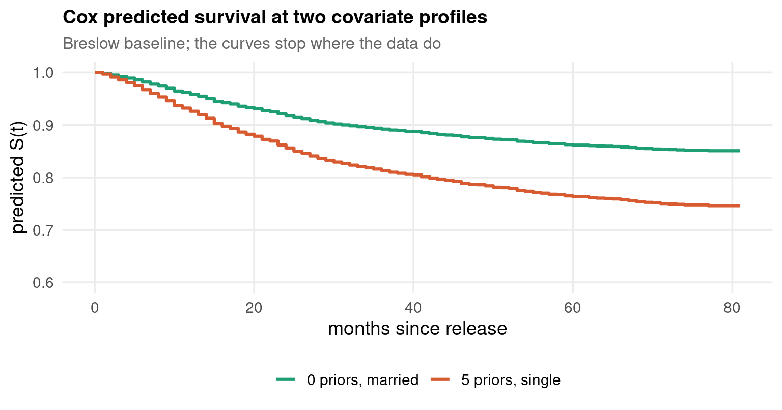
Code
import numpy as np
import pandas as pd
import matplotlib.pyplot as plt
import wooldridge as woo
from lifelines import CoxPHFitter

rc = woo.data('recid').assign(fail=lambda d: 1 - d['cens'])
X = ['workprg', 'priors', 'tserved', 'felon', 'alcohol',
     'drugs', 'black', 'married', 'educ', 'age']
cp = CoxPHFitter().fit(rc[X + ['durat', 'fail']], 'durat', 'fail')

prof = pd.DataFrame({'workprg': [0, 0], 'priors': [0, 5], 'tserved': [12, 12],
                     'felon': [1, 1], 'alcohol': [0, 0], 'drugs': [0, 0],
                     'black': [0, 0], 'married': [1, 0], 'educ': [12, 12],
                     'age': [360, 360]})
sf = cp.predict_survival_function(prof)

fig, ax = plt.subplots(figsize=(8, 4.2))
t = np.r_[0.0, sf.index.values]
for col, lab, c in [(0, "0 priors, married", "#1D9E75"),
                    (1, "5 priors, single",  "#D85A30")]:
    ax.step(t, np.r_[1.0, sf.iloc[:, col].values], where="post",
            color=c, lw=1.8, label=lab)
ax.text(0.03, 0.10, "S(60): %.4f  vs  %.4f"
        % (np.interp(60, sf.index.values, sf.iloc[:, 0].values),
           np.interp(60, sf.index.values, sf.iloc[:, 1].values)),
        transform=ax.transAxes, fontsize=10, color="#185FA5")
axopts = ax.set(xlim=(0, 81), ylim=(0.6, 1.0), xticks=range(0, 81, 20),
                yticks=np.arange(0.6, 1.01, 0.1),
                xlabel="months since release", ylabel="predicted S(t)",
                title="Cox predicted survival at two covariate profiles")
ax.legend(frameon=False, loc="lower left")
plt.show()
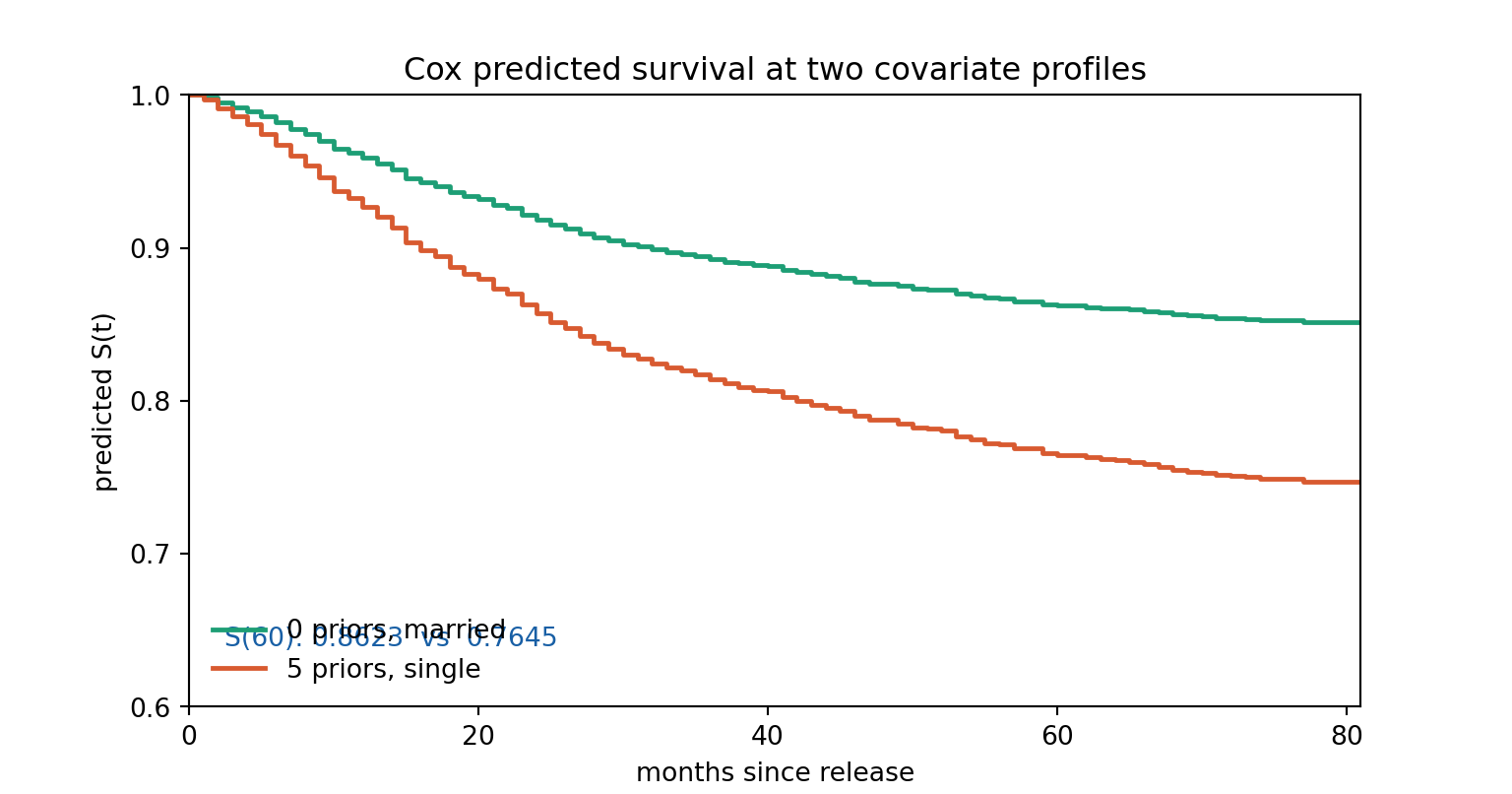
Code
quietly frause recid, clear
gen fail = 1 - cens
quietly stset durat, failure(fail == 1)
quietly stcox workprg priors tserved felon alcohol drugs black married educ age, efron

* stcurve inherits the fitted model; at() sets the covariate profile
stcurve, survival at(workprg=0 priors=0 tserved=12 felon=1 alcohol=0 drugs=0  ///
                     black=0 married=1 educ=12 age=360)                       ///
                 at(workprg=0 priors=5 tserved=12 felon=1 alcohol=0 drugs=0   ///
                     black=0 married=0 educ=12 age=360)                       ///
    connect(stairstep stairstep)                                              ///
    plot1opts(lcolor("29 158 117") lwidth(medthick))                          ///
    plot2opts(lcolor("216 90 48")  lwidth(medthick))                          ///
    xscale(range(0 81)) xlabel(0(20)80)                                       ///
    yscale(range(0.6 1)) ylabel(0.6(0.1)1)                                    ///
    xtitle("months since release") ytitle("predicted S(t)")                   ///
    title("Cox predicted survival at two covariate profiles", size(medium))   ///
    subtitle("Breslow baseline; the curves stop where the data do", size(small)) ///
    legend(order(1 "0 priors, married" 2 "5 priors, single") rows(1)          ///
           position(6) ring(1) region(lstyle(none)))                                              ///
    graphregion(color(white)) plotregion(color(white)) xsize(8) ysize(4.2)
graph export "../plots/dsc-p3-base.png", replace width(1600)
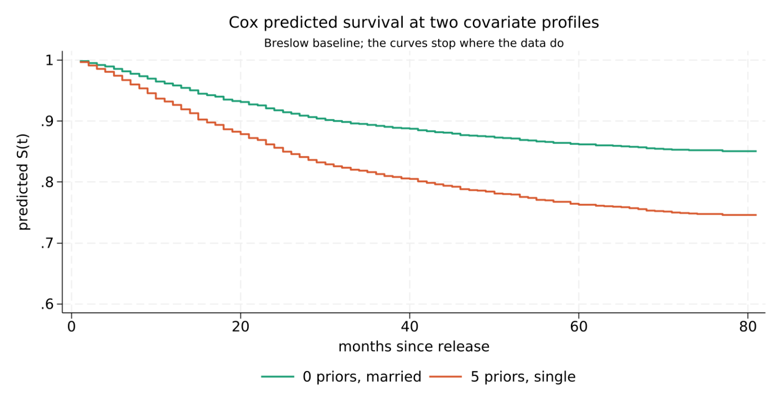
A 30-year-old with no priors and a wife has predicted survival \(0.8616\) at five years; the same man with five priors and no wife has \(0.7632\). That is the model’s whole content in one comparison, and it is the number to put in front of an audience rather than a table of hazard ratios.

Both curves stop at month 81. Asking what happens at month 100 requires a functional form, and supplying one is what Part 4 is for.

Part 4 — Parametric Duration

Weibull and friends; proportional hazards versus accelerated failure time

Why Go Parametric at All

Part 3 gave hazard ratios without committing to a shape for \(h_0\). Giving up that freedom has to buy something.

The Cox model’s \(\hat H_0\) ends at the last observed event — month 81 in recid. Beyond that it says nothing at all, and no amount of data manipulation changes that.

A parametric model has \(H_0(t)\) defined for every \(t\), so it answers the questions policy actually asks:

  • what fraction will have returned within ten years?
  • what is the median time to re-arrest, when the median is not reached in-sample?
  • what is the expected duration \(\mathbb{E}[T \mid \mathbf{x}] = \int_0^\infty S(u \mid \mathbf{x})\,du\)?

None of these is available from a Cox fit. Two slides from now the Weibull answers the second one — and the answer is a warning as much as a number.

The shape parameter is not a nuisance. In a search model the hazard is the re-employment rate, so \(p\) in

\[h(t) = p\,\lambda\,t^{\,p-1} e^{\mathbf{x}'\boldsymbol{\beta}}\]

is a statement about how search prospects evolve — skill depreciation, employer screening, benefit exhaustion. \(\hat p\) has an economic reading; a Breslow step function does not.

The same applies to the AFT parameterisation, where coefficients answer “by what factor does this stretch the spell?” — the question labour economists usually mean.

If the family is right, maximum likelihood is efficient and Cox is not. If it is wrong, Cox is consistent and ML is not. That is the entire trade, and it is quantifiable:

On recid the Cox standard errors are 0.9958 to 1.0021 times the Weibull ones — the partial likelihood gives up at most two parts in a thousand. That is the price of not having to know the shape, and on this data it is close to free. The last slide of this part makes the comparison properly, including the delta-method correction the conversion needs.

The family is an assumption, and a testable one. The Weibull forces the hazard to be monotone: it cannot rise then fall, so it cannot represent a spell where prospects improve while a programme runs and worsen afterwards.

Extrapolation is only as good as the family. A Weibull fitted to 81 months of data will happily report a median at month 462 — with a confidence interval — and nothing in the data supports the shape out there.

The Families

Family Hazard \(h(t)\) Shape of the hazard
Exponential \(\lambda\) flat; memoryless
Weibull \(p\lambda t^{p-1}\) monotone: falling if \(p<1\), rising if \(p>1\)
Gompertz \(\lambda e^{\gamma t}\) monotone, exponentially so; \(\gamma<0\) falling
Log-normal non-closed form hump-shaped: rises then falls
Log-logistic \(\dfrac{(1/\sigma)\,t^{1/\sigma-1}}{\gamma^{1/\sigma}\big[1+(t/\gamma)^{1/\sigma}\big]}\) hump-shaped if \(\sigma<1\), falling if \(\sigma \ge 1\)
Generalised gamma non-closed form nests exponential, Weibull, log-normal, gamma

The distinction that matters is monotone versus not. Exponential, Weibull and Gompertz can only go one way. Log-normal and log-logistic can rise and then fall, which is what a spell with an initial honeymoon period looks like.

Three inputs, in decreasing order of authority.

1. The Nelson–Aalen shape from Part 2. \(\hat H\) on recid was clearly concave, so the hazard falls throughout: a monotone-declining family is defensible and a rising one is not.

2. Economics. If the story involves benefit exhaustion at a known date, no smooth family captures it and a discrete-time model with a dummy is better (Part 6). If the story is pure skill depreciation, monotone decline is the prediction.

3. AIC, last. Two slides from now. It is a tiebreaker between defensible families, never a substitute for the first two.

The generalised gamma looks like the obvious answer — nest everything and let the data pick. On recid it does not converge to an interior maximum: the Hessian is not positive definite and the reported shape sits on a boundary. It is excluded from the horse race for that reason. Nesting families buys flexibility and pays in identification, which is Part 5’s theme in a different costume.

Proportional Hazards versus Accelerated Failure Time

Proportional hazards multiplies the hazard:

\[h(t \mid \mathbf{x}) = h_0(t)\,\exp(\mathbf{x}'\boldsymbol{\beta}_{\text{PH}})\]

Accelerated failure time stretches the clock:

\[\log T = \mathbf{x}'\boldsymbol{\beta}_{\text{AFT}} + \sigma\,\varepsilon \qquad\Longleftrightarrow\qquad S(t \mid \mathbf{x}) = S_0\!\left(t\,e^{-\mathbf{x}'\boldsymbol{\beta}_{\text{AFT}}}\right)\]

AFT says a covariate makes time pass faster or slower. It is a log-linear regression on the duration with a censored dependent variable, so its coefficients read like OLS coefficients: \(\beta_{\text{AFT}} = 0.19\) for married means married men’s spells are \(e^{0.19} = 1.21\) times longer, a 21% longer time to re-arrest.

Economists usually want the AFT reading; the survival literature usually reports PH. They are not rival models — for the Weibull they are the same model in two coordinate systems.

For the Weibull, and only because the Weibull is both, the two sets of coefficients are related by the shape parameter:

\[\boxed{\;\boldsymbol{\beta}_{\text{PH}} = -\,p \cdot \boldsymbol{\beta}_{\text{AFT}}\;} \qquad p = \frac{1}{\sigma}\]

The sign flip is the whole intuition: raising the hazard shortens the spell. The factor \(p\) converts between “rate” units and “time” units.

Check it on recid, where \(\hat p = 0.805864\):

\[\hat\beta_{\text{AFT}}^{\text{workprg}} = -0.112773 \;\Longrightarrow\; \hat\beta_{\text{PH}}^{\text{workprg}} = -0.805864 \times (-0.112773) = 0.090873\]

which is what the Cox model gave to two decimals (\(0.084405\)) without assuming any family at all.

Family PH AFT Note
Exponential the intersection is trivial: \(p = 1\)
Weibull the only non-trivial family that is both
Gompertz PH only; standard in mortality work
Log-normal AFT only, hump-shaped hazard
Log-logistic AFT only, hump-shaped hazard
Generalised gamma AFT only
Cox PH with \(h_0\) unspecified

This table explains a lot of confusion in applied papers. If a referee asks for “the hazard ratio” from a log-normal fit, the honest answer is that there is no such number — the ratio is not constant in \(t\), so any single figure is an average over an unstated weighting.

Software defaults differ. Stata’s streg reports PH for families that have one and AFT otherwise, switching on the time option. R’s survreg only ever reports AFT. lifelines names its classes ...AFTFitter, so it is explicit. Read the sign before reading the number.

Weibull in Both Parameterisations

Code
library(survival)
data("recid", package = "wooldridge")
recid <- transform(recid, fail = 1 - cens)

# survreg ALWAYS reports AFT; the PH coefficients are derived
w <- survreg(Surv(durat, fail) ~ workprg + priors + tserved + felon + alcohol +
               drugs + black + married + educ + age,
             data = recid, dist = "weibull")
print(summary(w))

p <- 1 / w$scale
both <- data.frame(AFT = round(coef(w)[-1], 6),
                   PH  = round(-coef(w)[-1] * p, 6))
cat("\nshape p = 1/scale =", round(p, 6), "\n\n")
print(both)

Call:
survreg(formula = Surv(durat, fail) ~ workprg + priors + tserved + 
    felon + alcohol + drugs + black + married + educ + age, data = recid, 
    dist = "weibull")
                Value Std. Error     z       p
(Intercept)  4.221670   0.341311 12.37 < 2e-16
workprg     -0.112785   0.112535 -1.00  0.3162
priors      -0.110176   0.017067 -6.46 1.1e-10
tserved     -0.016830   0.002130 -7.90 2.8e-15
felon        0.371623   0.131995  2.82  0.0049
alcohol     -0.555132   0.132243 -4.20 2.7e-05
drugs       -0.349265   0.121880 -2.87  0.0042
black       -0.563016   0.110817 -5.08 3.8e-07
married      0.188104   0.135752  1.39  0.1659
educ         0.028911   0.024115  1.20  0.2306
age          0.004622   0.000665  6.95 3.6e-12
Log(scale)   0.215840   0.038915  5.55 2.9e-08

Scale= 1.24 

Weibull distribution
Loglik(model)= -3192.1   Loglik(intercept only)= -3274.8
    Chisq= 165.48 on 10 degrees of freedom, p= 2.4e-30 
Number of Newton-Raphson Iterations: 5 
n= 1445 

shape p = 1/scale = 0.805864 
              AFT        PH
workprg -0.112785  0.090889
priors  -0.110176  0.088787
tserved -0.016830  0.013562
felon    0.371623 -0.299477
alcohol -0.555132  0.447361
drugs   -0.349265  0.281461
black   -0.563016  0.453715
married  0.188104 -0.151586
educ     0.028911 -0.023298
age      0.004622 -0.003725
Code
import numpy as np
import pandas as pd
import wooldridge as woo
from lifelines import WeibullAFTFitter

rc = woo.data('recid').assign(fail=lambda d: 1 - d['cens'])
X = ['workprg', 'priors', 'tserved', 'felon', 'alcohol',
     'drugs', 'black', 'married', 'educ', 'age']

wa = WeibullAFTFitter().fit(rc[X + ['durat', 'fail']], 'durat', 'fail')

# lambda_ holds the AFT coefficients, rho_ the log shape
aft = wa.params_.loc['lambda_'].drop('Intercept')
p = float(np.exp(wa.params_.loc[('rho_', 'Intercept')]))

both = pd.DataFrame({'AFT': aft.round(6), 'PH': (-aft * p).round(6)})
txt = (wa.summary[['coef', 'se(coef)', 'z', 'p']].round(6).to_string() +
       "\n\nshape p = %.6f    log-likelihood = %.4f\n\n" % (p, wa.log_likelihood_) +
       both.to_string())

import sys
nw = sys.stdout.write(txt + "\n")
                       coef  se(coef)          z         p
param   covariate                                         
lambda_ age        0.004622  0.000665   6.952063  0.000000
        alcohol   -0.555125  0.132243  -4.197772  0.000027
        black     -0.563020  0.110817  -5.080620  0.000000
        drugs     -0.349275  0.121880  -2.865724  0.004161
        educ       0.028913  0.024115   1.198935  0.230553
        felon      0.371629  0.131995   2.815470  0.004871
        married    0.188094  0.135752   1.385575  0.165877
        priors    -0.110176  0.017067  -6.455340  0.000000
        tserved   -0.016830  0.002130  -7.900251  0.000000
        workprg   -0.112773  0.112535  -1.002116  0.316287
        Intercept  4.221661  0.341312  12.368937  0.000000
rho_    Intercept -0.215840  0.038915  -5.546464  0.000000

shape p = 0.805864    log-likelihood = -3192.1088

                AFT        PH
covariate                    
age        0.004622 -0.003725
alcohol   -0.555125  0.447355
black     -0.563020  0.453717
drugs     -0.349275  0.281468
educ       0.028913 -0.023300
felon      0.371629 -0.299482
married    0.188094 -0.151578
priors    -0.110176  0.088787
tserved   -0.016830  0.013563
workprg   -0.112773  0.090880
Code
sys.stdout.flush()
Code
quietly frause recid, clear
gen fail = 1 - cens
quietly stset durat, failure(fail == 1)
* streg reports PH by default for the Weibull; `time' switches to AFT
streg workprg priors tserved felon alcohol drugs black married educ age, ///
    dist(weibull) nohr nolog
streg workprg priors tserved felon alcohol drugs black married educ age, ///
    dist(weibull) time nolog
        Failure _d: fail==1
  Analysis time _t: durat

Weibull PH regression

No. of subjects =  1,445                                Number of obs =  1,445
No. of failures =    552
Time at risk    = 80,013
                                                        LR chi2(10)   = 165.48
Log likelihood = -1633.0325                             Prob > chi2   = 0.0000

------------------------------------------------------------------------------
          _t | Coefficient  Std. err.      z    P>|z|     [95% conf. interval]
-------------+----------------------------------------------------------------
     workprg |   .0908893   .0906478     1.00   0.316    -.0867772    .2685558
      priors |   .0887867   .0134355     6.61   0.000     .0624535    .1151198
     tserved |   .0135625   .0016808     8.07   0.000     .0102682    .0168567
       felon |  -.2994775    .105974    -2.83   0.005    -.5071826   -.0917723
     alcohol |   .4473611   .1057353     4.23   0.000     .2401236    .6545985
       drugs |   .2814605   .0978644     2.88   0.004     .0896499    .4732711
       black |   .4537147   .0883037     5.14   0.000     .2806426    .6267867
     married |  -.1515864   .1092454    -1.39   0.165    -.3657035    .0625307
        educ |  -.0232984   .0194196    -1.20   0.230    -.0613601    .0147633
         age |  -.0037246    .000525    -7.09   0.000    -.0047536   -.0026956
       _cons |  -3.402094   .3010177   -11.30   0.000    -3.992077    -2.81211
-------------+----------------------------------------------------------------
       /ln_p |  -.2158398   .0389149    -5.55   0.000    -.2921115   -.1395681
-------------+----------------------------------------------------------------
           p |   .8058644   .0313601                      .7466852    .8697338
         1/p |   1.240904   .0482896                      1.149777    1.339252
------------------------------------------------------------------------------

        Failure _d: fail==1
  Analysis time _t: durat

Weibull AFT regression

No. of subjects =  1,445                                Number of obs =  1,445
No. of failures =    552
Time at risk    = 80,013
                                                        LR chi2(10)   = 165.48
Log likelihood = -1633.0325                             Prob > chi2   = 0.0000

------------------------------------------------------------------------------
          _t | Coefficient  Std. err.      z    P>|z|     [95% conf. interval]
-------------+----------------------------------------------------------------
     workprg |  -.1127848   .1125346    -1.00   0.316    -.3333486     .107779
      priors |  -.1101757   .0170675    -6.46   0.000    -.1436273   -.0767241
     tserved |  -.0168297   .0021303    -7.90   0.000     -.021005   -.0126544
       felon |   .3716227   .1319951     2.82   0.005      .112917    .6303284
     alcohol |   -.555132   .1322427    -4.20   0.000    -.8143229    -.295941
       drugs |  -.3492654   .1218801    -2.87   0.004    -.5881461   -.1103847
       black |  -.5630162    .110817    -5.08   0.000    -.7802135   -.3458189
     married |   .1881041   .1357519     1.39   0.166    -.0779647    .4541729
        educ |   .0289111   .0241153     1.20   0.231    -.0183541    .0761763
         age |   .0046219   .0006648     6.95   0.000     .0033189    .0059249
       _cons |    4.22167   .3413114    12.37   0.000     3.552712    4.890628
-------------+----------------------------------------------------------------
       /ln_p |  -.2158398   .0389149    -5.55   0.000    -.2921115   -.1395681
-------------+----------------------------------------------------------------
           p |   .8058644   .0313601                      .7466852    .8697338
         1/p |   1.240904   .0482896                      1.149777    1.339252
------------------------------------------------------------------------------

The AFT coefficients agree to six decimals across all three: workprg \(-0.112773\), priors \(-0.110176\), black \(-0.563016\), intercept \(4.221661\), \(\log p = -0.215840\).

The log-likelihoods do not agree, and that is not an error. R and lifelines report \(-3192.1088\); Stata reports \(-1633.0325\). The gap is exactly \(\sum_{i: d_i = 1} \log t_i = 1559.0764\), because Stata’s streg reports the likelihood in the log-time metric while R and lifelines report it for the density of \(T\) itself. Both are valid; only one thing follows. Compare likelihoods and AICs within a package, never across. The next slide reports \(\Delta\)AIC for exactly this reason, and the ranking is identical everywhere.

The Family Horse Race

Five families, one specification, ranked by \(\Delta\)AIC against the best.

Code
library(survival)
library(flexsurv)
data("recid", package = "wooldridge")
recid <- transform(recid, fail = 1 - cens)

f <- Surv(durat, fail) ~ workprg + priors + tserved + felon + alcohol +
  drugs + black + married + educ + age

race <- NULL
for (d in c("exponential", "weibull", "lognormal", "loglogistic")) {
  m <- survreg(f, data = recid, dist = d)
  k <- length(coef(m)) + (d != "exponential")
  race <- rbind(race, data.frame(family = d, logL = m$loglik[2], k = k,
                                 AIC = -2 * m$loglik[2] + 2 * k))
}
# Gompertz is PH-only, so survreg cannot fit it; flexsurv can
g <- flexsurvreg(f, data = recid, dist = "gompertz")
race <- rbind(race, data.frame(family = "gompertz", logL = g$loglik,
                               k = g$npars, AIC = g$AIC))

race <- transform(race, dAIC = round(AIC - min(AIC), 3))
race <- race[order(race$dAIC), ]
print(transform(race, logL = round(logL, 4), AIC = round(AIC, 3)),
      row.names = FALSE)
      family      logL  k      AIC    dAIC
    gompertz -3154.662 12 6333.323   0.000
   lognormal -3156.135 12 6336.271   2.947
 loglogistic -3170.019 12 6364.039  30.716
     weibull -3192.109 12 6408.218  74.894
 exponential -3208.829 11 6439.659 106.336
Code
import numpy as np
import pandas as pd
import wooldridge as woo
import statsmodels.api as sm
from scipy.optimize import minimize
from scipy.stats import norm

rc = woo.data('recid').assign(fail=lambda d: 1 - d['cens'])
xn = ['workprg', 'priors', 'tserved', 'felon', 'alcohol',
      'drugs', 'black', 'married', 'educ', 'age']
X = sm.add_constant(rc[xn]).values
t = rc['durat'].values.astype(float)
d = rc['fail'].values.astype(float)
lt = np.log(t)

# lifelines covers Weibull, log-normal and log-logistic but not exponential
# or Gompertz regression, so all five are hand-coded here for one common scale.
# Each returns (log density, log survivor); th[0] is the shape where there is one.
def exponential(th):
    xb = X @ th
    return xb - t * np.exp(xb), -t * np.exp(xb)

def weibull(th):
    p, xb = np.exp(th[0]), X @ th[1:]
    H = t**p * np.exp(xb)
    return th[0] + (p - 1) * lt + xb - H, -H

def gompertz(th):
    g, xb = th[0], X @ th[1:]
    H = (np.exp(g * t) - 1) / g * np.exp(xb)
    return g * t + xb - H, -H

def lognormal(th):
    s = np.exp(th[0]); z = (lt - X @ th[1:]) / s
    return norm.logpdf(z) - np.log(t * s), norm.logsf(z)

def loglogistic(th):
    s = np.exp(th[0]); z = (lt - X @ th[1:]) / s
    return -z - np.log(s * t) - 2 * np.logaddexp(0, -z), -np.logaddexp(0, z)

k = X.shape[1]
fams = [("exponential",  exponential,  0, np.r_[-4.0, np.zeros(k - 1)]),
        ("weibull",      weibull,      1, np.r_[0.0, -4.0, np.zeros(k - 1)]),
        ("lognormal",    lognormal,    1, np.r_[0.0,  4.0, np.zeros(k - 1)]),
        ("loglogistic",  loglogistic,  1, np.r_[0.0,  4.0, np.zeros(k - 1)]),
        ("gompertz",     gompertz,     1, np.r_[-0.01, -4.0, np.zeros(k - 1)])]

rows = []
for name, fam, extra, start in fams:
    def nll(th, fam=fam):
        lf, lS = fam(th)
        return -np.sum(d * lf + (1 - d) * lS)
    r = minimize(nll, start, method="BFGS", options={"maxiter": 60000, "gtol": 1e-9})
    r = minimize(nll, r.x, method="Nelder-Mead",
                 options={"maxiter": 200000, "maxfev": 200000,
                          "fatol": 1e-11, "xatol": 1e-11})
    npar = k + extra
    rows.append((name, round(-r.fun, 4), npar, round(2 * r.fun + 2 * npar, 3)))

race = pd.DataFrame(rows, columns=["family", "logL", "k", "AIC"])
race["dAIC"] = (race["AIC"] - race["AIC"].min()).round(3)

import sys
nw = sys.stdout.write(race.sort_values("dAIC").to_string(index=False) + "\n")
     family       logL  k      AIC    dAIC
   gompertz -3154.6600 12 6333.320   0.000
  lognormal -3156.1353 12 6336.271   2.951
loglogistic -3170.0195 12 6364.039  30.719
    weibull -3192.1088 12 6408.218  74.898
exponential -3208.8295 11 6439.659 106.339
Code
sys.stdout.flush()
Code
quietly frause recid, clear
gen fail = 1 - cens
quietly stset durat, failure(fail == 1)

foreach d in exp weibull lnormal llogistic gompertz {
    quietly streg workprg priors tserved felon alcohol drugs black married ///
        educ age, dist(`d') nolog
    scalar aic_`d' = -2 * e(ll) + 2 * e(k)
    display "`d'" _col(14) "logL = " %10.4f e(ll) "   k = " e(k) ///
            "   AIC = " %10.3f aic_`d'
}
scalar best = min(aic_exp, aic_weibull, aic_lnormal, aic_llogistic, aic_gompertz)
display _newline "dAIC against the best model"
foreach d in exp weibull lnormal llogistic gompertz {
    display "`d'" _col(14) %8.3f aic_`d' - best
}
  3.     scalar aic_`d' = -2 * e(ll) + 2 * e(k)
  4.     display "`d'" _col(14) "logL = " %10.4f e(ll) "   k = " e(k) ///
>             "   AIC = " %10.3f aic_`d'
  5. }
exp          logL = -1649.7531   k = 11   AIC =   3321.506
weibull      logL = -1633.0325   k = 12   AIC =   3290.065
lnormal      logL = -1597.0590   k = 12   AIC =   3218.118
llogistic    logL = -1610.9431   k = 12   AIC =   3245.886
gompertz     logL = -1595.5837   k = 12   AIC =   3215.167


dAIC against the best model

exp           106.339
weibull        74.898
lnormal         2.951
llogistic      30.719
gompertz        0.000

The ranking is identical in all three languages, and so is every \(\Delta\)AIC: Gompertz \(0\), log-normal \(2.951\), log-logistic \(30.719\), Weibull \(74.898\), exponential \(106.339\). The AIC levels differ between Stata and the other two by the constant of the previous slide, which is exactly why the comparison is stated in differences.

Two readings, one statistical and one economic.

Statistically, Gompertz and log-normal are within \(3\) AIC points of each other and cannot be separated; both beat the Weibull decisively. The exponential — constant hazard, no duration dependence — is dead by \(106\) points.

Economically, they tell different stories. Gompertz has an exponentially falling hazard throughout. Log-normal has a hazard that rises for the first few months and then falls. The data cannot choose between them, and only a model of what happens after release can.

The Shape Parameter as a Test

Inside the Weibull, duration dependence is one parameter and one test:

\[H_0: p = 1 \quad\text{(constant hazard, exponential)} \qquad\text{versus}\qquad H_1: p \ne 1\]

Every package tests it on the log scale, where the sampling distribution is far closer to normal and the null becomes a zero restriction:

\[z = \frac{\log \hat p}{\mathrm{se}(\log \hat p)} \;\overset{a}{\sim}\; \mathcal{N}(0,1)\]

Stata calls the parameter /ln_p, R stores \(-\log(\hat\sigma)\), and lifelines names it rho_. They are the same number.

Code
data("recid", package = "wooldridge")
recid <- transform(recid, fail = 1 - cens)
w <- survreg(Surv(durat, fail) ~ workprg + priors + tserved + felon + alcohol +
               drugs + black + married + educ + age,
             data = recid, dist = "weibull")

lnp <- -log(w$scale)                       # survreg stores log(scale)
se  <- sqrt(w$var[nrow(w$var), ncol(w$var)])

cat("log p =", round(lnp, 6), "  se =", round(se, 6),
    "\np     =", round(exp(lnp), 6),
    "  95% CI [", round(exp(lnp - 1.96 * se), 6), ",",
    round(exp(lnp + 1.96 * se), 6), "]",
    "\nz for H0: p = 1 :", round(lnp / se, 4),
    "  p-value =", format.pval(2 * pnorm(-abs(lnp / se)), digits = 4), "\n")
log p = -0.21584   se = 0.038915 
p     = 0.805864   95% CI [ 0.746684 , 0.869735 ] 
z for H0: p = 1 : -5.5465   p-value = 2.915e-08 
Code
import numpy as np
import wooldridge as woo
from lifelines import WeibullAFTFitter

rc = woo.data('recid').assign(fail=lambda d: 1 - d['cens'])
X = ['workprg', 'priors', 'tserved', 'felon', 'alcohol',
     'drugs', 'black', 'married', 'educ', 'age']
wa = WeibullAFTFitter().fit(rc[X + ['durat', 'fail']], 'durat', 'fail')

# lifelines calls log p "rho_"; the reported z tests rho_ = 0, i.e. p = 1
r = wa.summary.loc[('rho_', 'Intercept')]
txt = ("log p = %.6f   se = %.6f\np     = %.6f   95%% CI [ %.6f , %.6f ]\n"
       "z for H0: p = 1 : %.4f   p-value = %.3g"
       % (r['coef'], r['se(coef)'], np.exp(r['coef']),
          np.exp(r['coef lower 95%']), np.exp(r['coef upper 95%']),
          r['z'], r['p']))

import sys
nw = sys.stdout.write(txt + "\n")
log p = -0.215840   se = 0.038915
p     = 0.805864   95% CI [ 0.746685 , 0.869734 ]
z for H0: p = 1 : -5.5465   p-value = 2.92e-08
Code
sys.stdout.flush()
Code
quietly frause recid, clear
gen fail = 1 - cens
quietly stset durat, failure(fail == 1)
quietly streg workprg priors tserved felon alcohol drugs black married educ age, ///
    dist(weibull) nolog
* /ln_p is log p; the z on that row tests p = 1
display "log p = " _b[/ln_p] "   se = " _se[/ln_p]
display "p     = " exp(_b[/ln_p])
display "z for H0: p = 1 : " _b[/ln_p] / _se[/ln_p]
* the exponential is the p = 1 restriction, so an LR test says the same thing.
* `force' is needed because Stata files streg dist(weibull) and dist(exp) as
* different estimators (weibull vs ereg) and refuses to compare them otherwise.
estimates store weib
quietly streg workprg priors tserved felon alcohol drugs black married educ age, ///
    dist(exp) nolog
estimates store expo
lrtest weib expo, force
log p = -.21583983   se = .03891485

p     = .80586436

z for H0: p = 1 : -5.5464638


Likelihood-ratio test
Assumption: expo nested within weib

 LR chi2(1) =  33.44
Prob > chi2 = 0.0000

\(\hat p = 0.805864\) with a 95% interval of \([0.746685,\, 0.869734]\), and \(z = -5.5465\) against \(p = 1\). The interval excludes 1 comfortably; the likelihood ratio against the exponential is \(33.4\) on 1 df.

Taken at face value this is strong negative duration dependence: a man’s monthly risk of returning to prison falls the longer he stays out.

Do not take it at face value. Part 5 fits exactly this model to data built with a constant hazard by construction, and recovers \(\hat p = 0.743\) with a comparable \(z\). Unmodelled heterogeneity manufactures this result. A significant \(\hat p < 1\) is a starting point for an argument, never the end of one.

Predicted Median Duration

For a Weibull AFT the quantiles are closed-form. The median solves \(S(t) = 0.5\):

\[\hat t_{0.5}(\mathbf{x}) = \exp\!\big(\mathbf{x}'\hat{\boldsymbol{\beta}}_{\text{AFT}}\big) \cdot (\log 2)^{1/\hat p}\]

A confidence interval follows from the linear predictor, whose standard error the software supplies, because the transformation is monotone:

\[\Big[\exp\!\big(\hat\eta - 1.96\,\mathrm{se}(\hat\eta)\big),\; \exp\!\big(\hat\eta + 1.96\,\mathrm{se}(\hat\eta)\big)\Big] \cdot (\log 2)^{1/\hat p}, \qquad \hat\eta = \mathbf{x}'\hat{\boldsymbol{\beta}}_{\text{AFT}}\]

This is the number the Cox model of Part 3 could not produce, because the median was never reached in-sample.

Code
data("recid", package = "wooldridge")
recid <- transform(recid, fail = 1 - cens)
w <- survreg(Surv(durat, fail) ~ workprg + priors + tserved + felon + alcohol +
               drugs + black + married + educ + age,
             data = recid, dist = "weibull")

# the same two profiles as the Cox slide; age is in MONTHS
prof <- data.frame(workprg = 0, priors = c(0, 5), tserved = 12, felon = 1,
                   alcohol = 0, drugs = 0, black = 0, married = c(1, 0),
                   educ = 12, age = 360)

lp <- predict(w, newdata = prof, type = "lp", se.fit = TRUE)
p  <- 1 / w$scale
fac <- log(2)^(1 / p)

out <- data.frame(
  profile = c("0 priors, married", "5 priors, single"),
  median  = round(exp(lp$fit) * fac, 2),
  lower   = round(exp(lp$fit - 1.96 * lp$se.fit) * fac, 2),
  upper   = round(exp(lp$fit + 1.96 * lp$se.fit) * fac, 2))
print(out, row.names = FALSE)
cat("\nlongest observed spell in the data:", max(recid$durat), "months\n")
           profile median  lower  upper
 0 priors, married 461.94 300.47 710.20
  5 priors, single 220.62 151.27 321.77

longest observed spell in the data: 81 months
Code
import numpy as np
import pandas as pd
import wooldridge as woo
from lifelines import WeibullAFTFitter

rc = woo.data('recid').assign(fail=lambda d: 1 - d['cens'])
X = ['workprg', 'priors', 'tserved', 'felon', 'alcohol',
     'drugs', 'black', 'married', 'educ', 'age']
wa = WeibullAFTFitter().fit(rc[X + ['durat', 'fail']], 'durat', 'fail')

prof = pd.DataFrame({'workprg': [0, 0], 'priors': [0, 5], 'tserved': [12, 12],
                     'felon': [1, 1], 'alcohol': [0, 0], 'drugs': [0, 0],
                     'black': [0, 0], 'married': [1, 0], 'educ': [12, 12],
                     'age': [360, 360]})

b = wa.params_.loc['lambda_']
V = wa.variance_matrix_.loc['lambda_', 'lambda_']
# lifelines stores parameters alphabetically, so align the design matrix to
# b.index rather than to X -- getting this wrong is silent and catastrophic
Z = prof.assign(Intercept=1.0)[b.index].values
eta = Z @ b.values
se = np.sqrt(np.einsum('ij,jk,ik->i', Z, V.values, Z))
p = float(np.exp(wa.params_.loc[('rho_', 'Intercept')]))
fac = np.log(2) ** (1 / p)

out = pd.DataFrame({'profile': ["0 priors, married", "5 priors, single"],
                    'median': (np.exp(eta) * fac).round(2),
                    'lower': (np.exp(eta - 1.96 * se) * fac).round(2),
                    'upper': (np.exp(eta + 1.96 * se) * fac).round(2)})
txt = (out.to_string(index=False) +
       "\n\nlongest observed spell in the data: %d months" % rc['durat'].max())

import sys
nw = sys.stdout.write(txt + "\n")
          profile  median  lower  upper
0 priors, married  461.94 300.47 710.20
 5 priors, single  220.63 151.27 321.78

longest observed spell in the data: 81 months
Code
sys.stdout.flush()
Code
quietly frause recid, clear
gen fail = 1 - cens
quietly stset durat, failure(fail == 1)
quietly streg workprg priors tserved felon alcohol drugs black married educ age, ///
    dist(weibull) time nolog

scalar p   = exp(_b[/ln_p])
scalar fac = (ln(2))^(1 / p)

* lincom gives the linear predictor and its standard error at a covariate
* profile; omitted terms are zero. Age is in MONTHS, so 360 is a 30-year-old.
quietly lincom _cons + 12*tserved + 1*felon + 12*educ + 360*age + 1*married
display "median (0 priors, married) = " %8.2f exp(r(estimate)) * fac         ///
        "   [" %8.2f exp(r(estimate) - 1.96*r(se)) * fac ", "                ///
              %8.2f exp(r(estimate) + 1.96*r(se)) * fac "]"

quietly lincom _cons + 5*priors + 12*tserved + 1*felon + 12*educ + 360*age
display "median (5 priors, single)  = " %8.2f exp(r(estimate)) * fac         ///
        "   [" %8.2f exp(r(estimate) - 1.96*r(se)) * fac ", "                ///
              %8.2f exp(r(estimate) + 1.96*r(se)) * fac "]"

quietly summarize durat
display _newline "longest observed spell in the data: " r(max) " months"
median (0 priors, married) =   461.94   [  300.47,   710.20]


median (5 priors, single)  =   220.62   [  151.27,   321.77]


longest observed spell in the data: 81 months

Read these numbers as a warning, not a result. The low-risk profile has a predicted median of 461.9 months — 38 years — with a 95% interval of \([300.5,\, 710.2]\). The data end at 81 months. Every month past 81 is the Weibull assumption talking, and the confidence interval measures only parameter uncertainty, not the risk that the family is wrong.

Extrapolation is what the parametric model buys, and it is bought on credit. Quote \(\hat S(t)\) inside the observation window, and treat anything outside it as a scenario rather than an estimate.

Parametric versus Cox

Code
data("recid", package = "wooldridge")
recid <- transform(recid, fail = 1 - cens)
f <- Surv(durat, fail) ~ workprg + priors + tserved + felon + alcohol +
  drugs + black + married + educ + age

cx <- coxph(f, data = recid, ties = "efron")
w  <- survreg(f, data = recid, dist = "weibull")
p  <- 1 / w$scale
k  <- length(coef(w))      # survreg stores coefficients then log(scale)

# beta_PH = -beta_AFT / scale depends on TWO estimates, so its standard error
# needs the delta method -- scaling se(beta_AFT) by p alone ignores the shape
# parameter's own variance and its covariance with beta_AFT.
ls <- log(w$scale)
se_wph <- numeric(k - 1)
for (j in 2:k) {
  g <- numeric(k + 1)
  g[j]     <- -exp(-ls)              # d beta_PH / d beta_AFT
  g[k + 1] <- coef(w)[j] * exp(-ls)  # d beta_PH / d log(scale)
  se_wph[j - 1] <- sqrt(as.numeric(t(g) %*% w$var %*% g))
}
se_cox <- sqrt(diag(vcov(cx)))

cmp <- data.frame(
  cox        = round(coef(cx), 5),
  weibull_PH = round(-coef(w)[-1] * p, 5),
  se_cox     = round(se_cox, 5),
  se_weibull = round(se_wph, 5),
  se_ratio   = round(se_cox / se_wph, 4))
print(cmp)

cat("\nlargest absolute coefficient gap:",
    round(max(abs(coef(cx) + coef(w)[-1] * p)), 5),
    "\nse ratio (Cox / Weibull): min", round(min(se_cox / se_wph), 4),
    " max", round(max(se_cox / se_wph), 4),
    " mean", round(mean(se_cox / se_wph), 4), "\n")
             cox weibull_PH  se_cox se_weibull se_ratio
workprg  0.08440    0.09089 0.09081    0.09065   1.0018
priors   0.08802    0.08879 0.01346    0.01344   1.0021
tserved  0.01307    0.01356 0.00168    0.00168   1.0011
felon   -0.28390   -0.29948 0.10612    0.10597   1.0013
alcohol  0.43300    0.44736 0.10572    0.10574   0.9999
drugs    0.27760    0.28146 0.09787    0.09786   1.0000
black    0.43506    0.45371 0.08838    0.08830   1.0008
married -0.15514   -0.15159 0.10921    0.10925   0.9997
educ    -0.02136   -0.02330 0.01945    0.01942   1.0013
age     -0.00361   -0.00372 0.00052    0.00052   0.9958

largest absolute coefficient gap: 0.01865 
se ratio (Cox / Weibull): min 0.9958  max 1.0021  mean 1.0004 

The Weibull PH coefficients sit within a few percent of the Cox ones — priors \(0.08879\) against \(0.08802\), black \(0.45371\) against \(0.43506\) — and every sign and significance verdict is unchanged.

The standard errors are the real comparison, and the Weibull ones must be built with the delta method\(\beta_{\text{PH}} = -\beta_{\text{AFT}}/\sigma\) depends on two estimates, so scaling \(\mathrm{se}(\beta_{\text{AFT}})\) by \(p\) alone silently omits the shape parameter’s variance and its covariance with \(\beta_{\text{AFT}}\).

Done properly, the Cox-to-Weibull ratio runs from \(0.9958\) to \(1.0021\), averaging \(1.0004\). The partial likelihood cost essentially nothing in precision — at most two parts in a thousand — because the Weibull’s extra structure amounts to one shape parameter and the sample is large.

That balance is data-specific, not a general law. Efficiency gains from a parametric family grow when the sample is small, censoring is heavy, or the family is genuinely right. Here none of the three bites.

Goal Use
Hazard ratios, minimal assumptions Cox — it is the default for a reason
Survival probabilities inside the window either; they agree closely
Extrapolation, median duration, \(\mathbb{E}[T]\) parametric, and state the family
The shape of duration dependence is the question parametric, then read Part 5 before believing \(\hat p\)
Time-varying covariates Cox — the counting-process form is natural
Small samples, heavy censoring parametric, where the efficiency gain is real
Non-monotone hazard suspected log-normal or log-logistic; the Weibull cannot

The professional habit is to fit both and say so. If the Cox and parametric coefficients agree, the family assumption is doing no harm and the extra output — medians, extrapolated survival — comes for free. If they disagree, the disagreement is the finding, and it usually points at the hazard shape or at the heterogeneity of Part 5.

Part 5 — Unobserved Heterogeneity

Frailty, and the duration dependence it manufactures

The Mover–Stayer Problem

Take a population with two types and no duration dependence whatsoever:

  • movers, half the population, constant hazard \(h = 0.15\) per month
  • stayers, the other half, constant hazard \(h = 0.03\) per month

Nobody’s individual hazard changes with time. Every spell is exponential.

Now watch the observed hazard, which is computed among those still at risk:

\[\bar{h}(t) = \frac{\pi\,h_1 e^{-h_1 t} + (1-\pi)\,h_2 e^{-h_2 t}} {\pi\,e^{-h_1 t} + (1-\pi)\,e^{-h_2 t}}\]

At \(t = 0\) it is the simple average, \(0.09\). By month 40 almost every mover has gone, so the survivors are nearly all stayers and \(\bar h\) has fallen to about \(0.031\) — a two-thirds decline in a world where no individual hazard moved at all.

This is not a small-sample problem, a bias that vanishes with more data, or a computational artefact. It is a composition effect, and it is present in the population. More data estimates \(\bar h(t)\) more precisely; it does not make \(\bar h(t)\) any closer to the individual hazard.

The result is completely general. Write \(v\) for unobserved heterogeneity entering multiplicatively, \(h(t \mid v) = v\,h_0(t)\). The observed hazard is

\[\bar h(t) = h_0(t)\;\mathbb{E}[\,v \mid T \ge t\,]\]

so its evolution has two parts: the true baseline, and the drift of the surviving population’s average frailty. And that drift is signed:

\[\frac{d}{dt}\,\mathbb{E}[\,v \mid T \ge t\,] = -\,h_0(t)\;\mathrm{Var}[\,v \mid T \ge t\,] \;\le\; 0\]

The conditional mean of frailty among survivors is always non-increasing, strictly so whenever there is any heterogeneity left. High-\(v\) units fail first, by construction.

Therefore the observed hazard is biased toward negative duration dependence always: \(\bar h\) understates \(h_0\)’s growth and overstates its decline. Positive duration dependence estimated without frailty is a lower bound on the truth; negative duration dependence is no evidence at all.

Code
t  <- seq(0, 40, by = 0.1)
h1 <- 0.15   # movers
h2 <- 0.03   # stayers
pi <- 0.5

# observed hazard = frailty-weighted average among the survivors
hbar <- (pi * h1 * exp(-h1 * t) + (1 - pi) * h2 * exp(-h2 * t)) /
        (pi * exp(-h1 * t) + (1 - pi) * exp(-h2 * t))

mix <- data.frame(
  t = rep(t, 3),
  h = c(rep(h1, length(t)), rep(h2, length(t)), hbar),
  series = factor(rep(c("movers (individual)", "stayers (individual)",
                        "observed, whole population"), each = length(t)),
                  levels = c("movers (individual)", "stayers (individual)",
                             "observed, whole population")))

ggplot(mix) +
  aes(x = t, y = h, colour = series) +
  geom_line(linewidth = 1.2) +
  scale_colour_manual(values = c("#1D9E75", "#185FA5", "#D85A30")) +
  coord_cartesian(xlim = c(0, 40), ylim = c(0, 0.17)) +
  scale_x_continuous(breaks = seq(0, 40, 10)) +
  scale_y_continuous(breaks = seq(0, 0.15, 0.05)) +
  labs(x = "months", y = "hazard", colour = NULL,
       title = "Two flat hazards, one falling observed hazard",
       subtitle = "no individual hazard changes; only the mix of survivors does")
observed hazard: h(0) = 0.09   h(20) = 0.03998   h(40) = 0.03098 
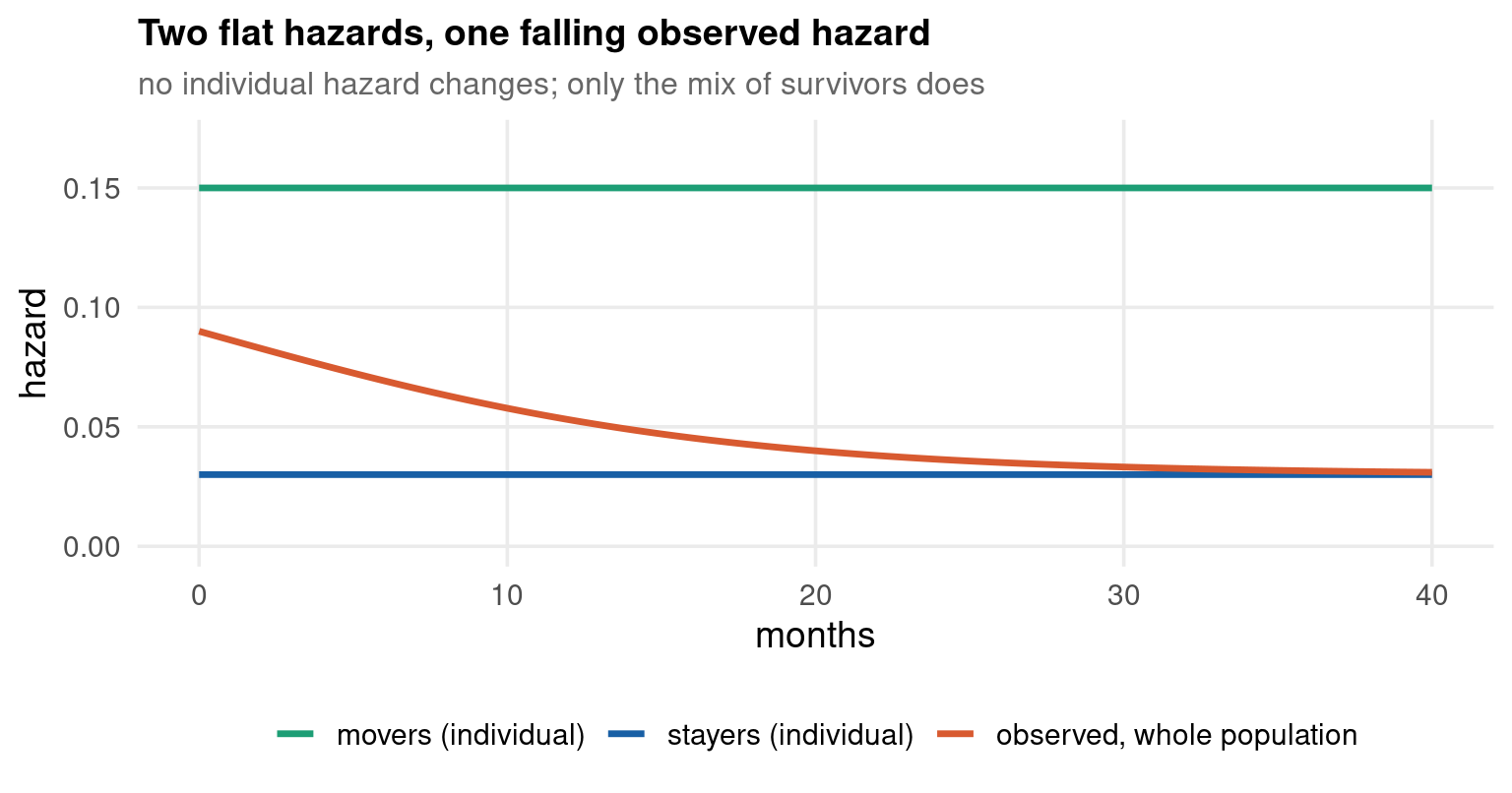
Code
import numpy as np
import matplotlib.pyplot as plt

t = np.arange(0, 40.01, 0.1)
h1, h2, pi = 0.15, 0.03, 0.5

hbar = (pi * h1 * np.exp(-h1 * t) + (1 - pi) * h2 * np.exp(-h2 * t)) / \
       (pi * np.exp(-h1 * t) + (1 - pi) * np.exp(-h2 * t))

fig, ax = plt.subplots(figsize=(8, 4.2))
ax.plot(t, np.full_like(t, h1), color="#1D9E75", lw=2, label="movers (individual)")
ax.plot(t, np.full_like(t, h2), color="#185FA5", lw=2, label="stayers (individual)")
ax.plot(t, hbar, color="#D85A30", lw=2, label="observed, whole population")
ax.text(0.35, 0.72, "observed hazard falls from %.3f to %.3f"
        % (hbar[0], hbar[-1]), transform=ax.transAxes,
        fontsize=10, color="#D85A30")
axopts = ax.set(xlim=(0, 40), ylim=(0, 0.17), xticks=range(0, 41, 10),
                yticks=np.arange(0, 0.16, 0.05), xlabel="months", ylabel="hazard",
                title="Two flat hazards, one falling observed hazard")
ax.legend(frameon=False, loc="upper right")
plt.show()
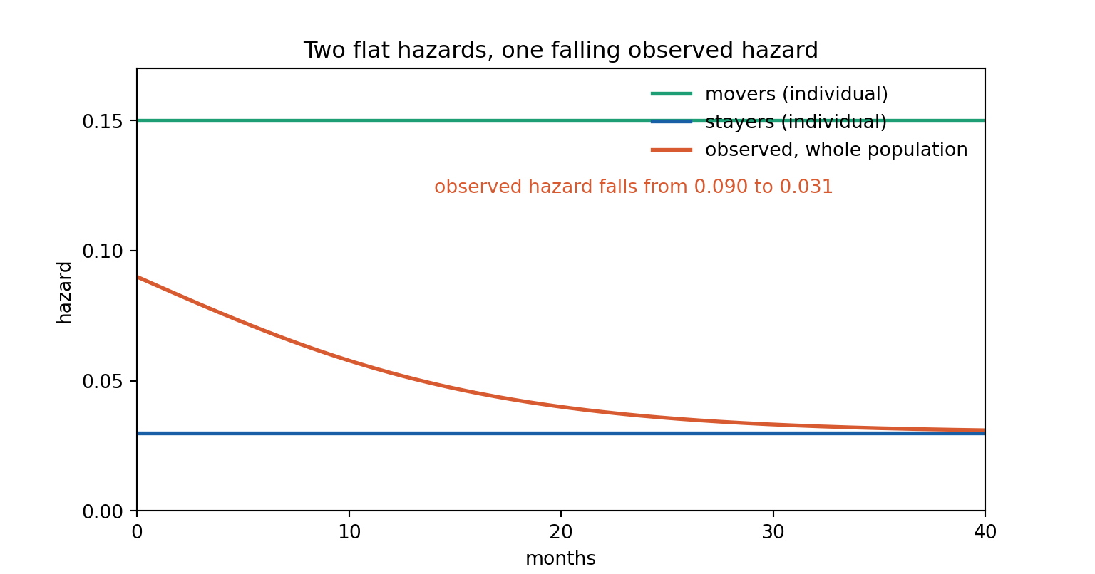
Code
clear
set obs 401
gen t = 0.1 * (_n - 1)
gen h1 = 0.15
gen h2 = 0.03
gen hbar = (0.5*0.15*exp(-0.15*t) + 0.5*0.03*exp(-0.03*t)) ///
         / (0.5*exp(-0.15*t) + 0.5*exp(-0.03*t))

twoway (line h1   t, lcolor("29 158 117") lwidth(medthick))                   ///
       (line h2   t, lcolor("24 95 165")  lwidth(medthick))                   ///
       (line hbar t, lcolor("216 90 48")  lwidth(medthick)),                  ///
    legend(order(1 "movers (individual)" 2 "stayers (individual)"             ///
                 3 "observed, whole population") rows(1) size(small)          ///
           position(6) ring(1) region(lstyle(none)))                                              ///
    xscale(range(0 40)) xlabel(0(10)40)                                       ///
    yscale(range(0 0.17)) ylabel(0(0.05)0.15)                                 ///
    xtitle("months") ytitle("hazard")                                         ///
    title("Two flat hazards, one falling observed hazard", size(medium))      ///
    subtitle("no individual hazard changes; only the mix of survivors does", size(small)) ///
    graphregion(color(white)) plotregion(color(white)) xsize(8) ysize(4.2)
graph export "../plots/dsc-p5-mix.png", replace width(1600)
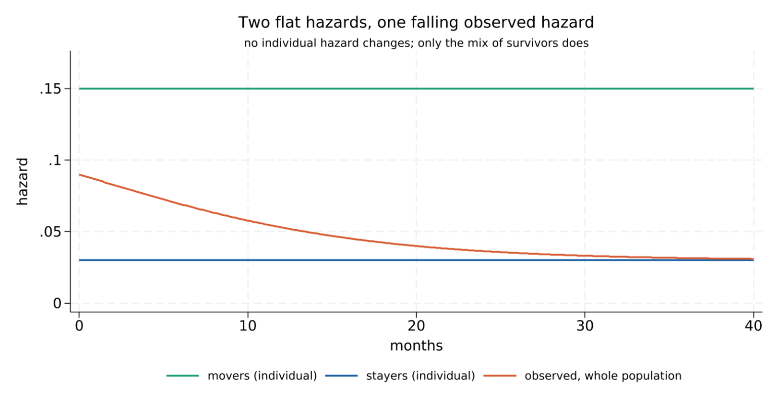
The Mixed Proportional Hazard Model

Add a multiplicative, unobserved, time-invariant term \(v_i > 0\) to the proportional hazard of Part 3:

\[h(t \mid \mathbf{x}_i, v_i) = v_i\; h_0(t)\, \exp(\mathbf{x}_i'\boldsymbol{\beta})\]

with \(v_i \perp \mathbf{x}_i\), \(\mathbb{E}[v] = 1\) as a normalisation, and \(\mathrm{Var}[v] = \theta\) the parameter of interest. Setting \(\theta = 0\) returns Part 4 exactly.

\(v\) is not observed, so it must be integrated out. The observed survivor function is the Laplace transform of the frailty distribution evaluated at the cumulative hazard:

\[S(t \mid \mathbf{x}) = \mathbb{E}_v\Big[ \exp\big(-v\,H_0(t) e^{\mathbf{x}'\boldsymbol{\beta}}\big)\Big] = \mathcal{L}_v\big(H_0(t) e^{\mathbf{x}'\boldsymbol{\beta}}\big)\]

That is why the choice of frailty distribution is a choice of Laplace transform — and why gamma is the workhorse.

For \(v \sim \mathrm{Gamma}\) with mean 1 and variance \(\theta\), the Laplace transform is elementary, and everything follows in closed form:

\[S(t \mid \mathbf{x}) = \Big[1 + \theta\, H_0(t)\, e^{\mathbf{x}'\boldsymbol{\beta}}\Big]^{-1/\theta}\]

\[\log L = \sum_{i=1}^{n}\Big[ d_i\big(\log h_0(t_i) + \mathbf{x}_i'\boldsymbol{\beta}\big) - \Big(\tfrac{1}{\theta} + d_i\Big) \log\!\big(1 + \theta H_0(t_i) e^{\mathbf{x}_i'\boldsymbol{\beta}}\big)\Big]\]

No numerical integration, no simulation — the whole model is fifteen lines of code, which is exactly what the Python tabs of this part do. The observed hazard is then

\[\bar h(t \mid \mathbf{x}) = \frac{h_0(t)e^{\mathbf{x}'\boldsymbol{\beta}}} {1 + \theta H_0(t) e^{\mathbf{x}'\boldsymbol{\beta}}}\]

which is visibly a declining function of \(t\) even for constant \(h_0\). That denominator is the whole story of this part.

Distribution Laplace transform Behaviour
Gamma closed form, \((1+\theta s)^{-1/\theta}\) the default; conjugate-like convenience, heavy right tail
Inverse Gaussian closed form lighter tail; survivors homogenise faster
Log-normal needs quadrature natural in multilevel models; no closed form
Discrete mass points trivial Heckman–Singer: no parametric assumption at all

The choice is not innocuous. Heckman & Singer (1984) showed that structural estimates can move substantially with the assumed frailty distribution, on the same data. Their proposal — a discrete distribution with a few mass points, estimated nonparametrically — has its own trouble: the number of points is itself hard to choose and the likelihood is often multimodal.

Practical position: report gamma because everyone does, then re-estimate with inverse-Gaussian and say whether the conclusion moved.

The Simulation: Fitting Without Frailty

dsc-frailty.csv is built with a constant baseline hazard, \(p = 1\) exactly. Any duration dependence a naive fit reports is manufactured.

\[\text{truth:}\quad p = 1, \quad \lambda = 0.04, \quad \beta_1 = -0.6, \quad \beta_2 = 0.4, \quad \theta = 2.5\]

Code
library(survival)
fr <- read.csv("../data/dsc-frailty.csv")

cat("n =", nrow(fr), " events =", sum(fr$event),
    " censored =", sum(1 - fr$event), "\n\n")

# ordinary Weibull, no frailty term -- exactly the Part 4 estimator
w <- survreg(Surv(time, event) ~ x1 + x2, data = fr, dist = "weibull")
p <- 1 / w$scale

est <- data.frame(
  parameter = c("p (shape)", "lambda", "beta1", "beta2"),
  truth     = c(1.0, 0.04, -0.60, 0.40),
  estimate  = round(c(p, exp(-coef(w)[1] * p), -coef(w)[2] * p, -coef(w)[3] * p), 6))
est <- transform(est, bias = round(estimate - truth, 6))
print(est, row.names = FALSE)

cat("\nz for H0: p = 1 :",
    round(-log(w$scale) / sqrt(w$var[nrow(w$var), ncol(w$var)]), 4), "\n")
n = 4000  events = 1604  censored = 2396 
 parameter truth  estimate      bias
 p (shape)  1.00  0.743427 -0.256573
    lambda  0.04  0.042846  0.002846
     beta1 -0.60 -0.389705  0.210295
     beta2  0.40  0.246533 -0.153467

z for H0: p = 1 : -12.7456 
Code
import numpy as np
import pandas as pd
from scipy.optimize import minimize

fr = pd.read_csv("../data/dsc-frailty.csv")
X = fr[['x1', 'x2']].values
t = fr['time'].values
d = fr['event'].values
lt = np.log(t)

# Weibull PH without frailty: log L = sum[ d*log h - H ]
def nll(th):
    p, lam, b = np.exp(th[0]), np.exp(th[1]), th[2:]
    xb = X @ b
    return -np.sum(d * (th[0] + (p - 1) * lt + th[1] + xb)
                   - t**p * np.exp(xb) * lam)

r = minimize(nll, [0.0, np.log(0.04), 0.0, 0.0], method='L-BFGS-B',
             options={'maxiter': 50000, 'ftol': 1e-16, 'gtol': 1e-12})
r = minimize(nll, r.x, method='BFGS', options={'maxiter': 50000, 'gtol': 1e-10})

est = pd.DataFrame({
    'parameter': ['p (shape)', 'lambda', 'beta1', 'beta2'],
    'truth': [1.0, 0.04, -0.60, 0.40],
    'estimate': np.round([np.exp(r.x[0]), np.exp(r.x[1]), r.x[2], r.x[3]], 6)})
est['bias'] = (est['estimate'] - est['truth']).round(6)

txt = ("n = %d  events = %d  censored = %d\n\n" % (len(fr), int(d.sum()), int((1 - d).sum())
       ) + est.to_string(index=False) +
       "\n\nlog-likelihood = %.4f" % -r.fun)

import sys
nw = sys.stdout.write(txt + "\n")
n = 4000  events = 1604  censored = 2396

parameter  truth  estimate      bias
p (shape)   1.00  0.743427 -0.256573
   lambda   0.04  0.042846  0.002846
    beta1  -0.60 -0.389705  0.210295
    beta2   0.40  0.246533 -0.153467

log-likelihood = -8154.5050
Code
sys.stdout.flush()
Code
quietly import delimited "../data/dsc-frailty.csv", clear
quietly destring _all, replace
stset time, failure(event == 1)
* no frailty() option: this is the ordinary Weibull of Part 4
streg x1 x2, dist(weibull) nolog
display _newline "truth:  p = 1   lambda = .04   HR(x1) = " exp(-0.6) ///
        "   HR(x2) = " exp(0.4)
Survival-time data settings

         Failure event: event==1
Observed time interval: (0, time]
     Exit on or before: failure

--------------------------------------------------------------------------
      4,000  total observations
          0  exclusions
--------------------------------------------------------------------------
      4,000  observations remaining, representing
      1,604  failures in single-record/single-failure data
 106,271.27  total analysis time at risk and under observation
                                                At risk from t =         0
                                     Earliest observed entry t =         0
                                          Last observed exit t =        36

        Failure _d: event==1
  Analysis time _t: time

Weibull PH regression

No. of subjects =       4,000                           Number of obs =  4,000
No. of failures =       1,604
Time at risk    = 106,271.266
                                                        LR chi2(2)    = 157.05
Log likelihood = -4899.288                              Prob > chi2   = 0.0000

------------------------------------------------------------------------------
          _t | Haz. ratio   Std. err.      z    P>|z|     [95% conf. interval]
-------------+----------------------------------------------------------------
          x1 |   .6772565   .0342734    -7.70   0.000     .6133058    .7478754
          x2 |   1.279582   .0316362     9.97   0.000     1.219054    1.343115
       _cons |   .0428459   .0028604   -47.19   0.000      .037591    .0488354
-------------+----------------------------------------------------------------
       /ln_p |  -.2964851   .0232618   -12.75   0.000    -.3420773   -.2508929
-------------+----------------------------------------------------------------
           p |   .7434267   .0172934                      .7102933    .7781057
         1/p |   1.345123   .0312899                      1.285172    1.407869
------------------------------------------------------------------------------
Note: _cons estimates baseline hazard.


truth:  p = 1   lambda = .04   HR(x1) = .54881164   HR(x2) = 1.4918247

\(\hat p = 0.743427\) against a truth of exactly 1. The shape parameter is \(5.6\) standard errors below one; a referee would call this decisive evidence of negative duration dependence. There is none in the data-generating process.

The covariate effects are wrong too, and in the direction that always happens: \(\hat\beta_1 = -0.3897\) against \(-0.6\), and \(\hat\beta_2 = 0.2465\) against \(0.4\) — both attenuated toward zero — by 35% and 38% respectively. Ignoring frailty does not only invent duration dependence; it shrinks every treatment effect you care about.

Recovering the Truth

The same data, the same three languages, one extra parameter — the frailty variance \(\theta\).

Code
fr <- read.csv("../data/dsc-frailty.csv")
X <- as.matrix(fr[, c("x1", "x2")])
t <- fr$time
d <- fr$event

# gamma-frailty MPH: the closed-form log-likelihood of the previous slide.
# par = (log p, log lambda, beta1, beta2, log theta)
negll <- function(par) {
  p   <- exp(par[1]); lam <- exp(par[2])
  th  <- exp(par[5]); xb  <- as.vector(X %*% par[3:4])
  A   <- 1 + th * lam * t^p * exp(xb)
  -sum(d * (par[1] + (p - 1) * log(t) + par[2] + xb) -
       (1 / th + d) * log(A))
}

o <- nlminb(c(0, log(0.04), 0, 0, 0), negll,
            control = list(iter.max = 5000, eval.max = 10000, rel.tol = 1e-15))

est <- data.frame(
  parameter = c("p (shape)", "lambda", "beta1", "beta2", "theta"),
  truth     = c(1.0, 0.04, -0.60, 0.40, 2.50),
  estimate  = round(c(exp(o$par[1]), exp(o$par[2]), o$par[3], o$par[4],
                      exp(o$par[5])), 6))
est <- transform(est, bias = round(estimate - truth, 6))
print(est, row.names = FALSE)

# likelihood ratio against the no-frailty fit of the previous slide
w <- survreg(Surv(time, event) ~ x1 + x2, data = fr, dist = "weibull")
cat("\nLR statistic for H0: theta = 0 :",
    round(2 * (-o$objective - w$loglik[2]), 4),
    "\n(chi-bar-squared: theta = 0 is on the boundary, so halve the p-value)\n")
 parameter truth  estimate      bias
 p (shape)  1.00  1.026187  0.026187
    lambda  0.04  0.036980 -0.003020
     beta1 -0.60 -0.658502 -0.058502
     beta2  0.40  0.391952 -0.008048
     theta  2.50  2.559869  0.059869

LR statistic for H0: theta = 0 : 62.3117 
(chi-bar-squared: theta = 0 is on the boundary, so halve the p-value)
Code
import numpy as np
import pandas as pd
from scipy.optimize import minimize

# lifelines has NO frailty model, so the MPH likelihood is coded directly.
# It is closed form for gamma frailty, so this costs about ten lines.
fr = pd.read_csv("../data/dsc-frailty.csv")
X = fr[['x1', 'x2']].values
t = fr['time'].values
d = fr['event'].values
lt = np.log(t)

# th = (log p, log lambda, beta1, beta2, log theta)
def nll(th):
    p, lam, q = np.exp(th[0]), np.exp(th[1]), np.exp(th[4])
    xb = X @ th[2:4]
    A = 1 + q * lam * t**p * np.exp(xb)
    return -np.sum(d * (th[0] + (p - 1) * lt + th[1] + xb)
                   - (1 / q + d) * np.log(A))

r = minimize(nll, [0.0, np.log(0.04), 0.0, 0.0, 0.0], method='L-BFGS-B',
             options={'maxiter': 50000, 'ftol': 1e-16, 'gtol': 1e-12})
r = minimize(nll, r.x, method='BFGS', options={'maxiter': 50000, 'gtol': 1e-10})

est = pd.DataFrame({
    'parameter': ['p (shape)', 'lambda', 'beta1', 'beta2', 'theta'],
    'truth': [1.0, 0.04, -0.60, 0.40, 2.50],
    'estimate': np.round([np.exp(r.x[0]), np.exp(r.x[1]),
                          r.x[2], r.x[3], np.exp(r.x[4])], 6)})
est['bias'] = (est['estimate'] - est['truth']).round(6)

txt = (est.to_string(index=False) +
       "\n\nlog-likelihood = %.4f" % -r.fun)

import sys
nw = sys.stdout.write(txt + "\n")
parameter  truth  estimate      bias
p (shape)   1.00  1.026186  0.026186
   lambda   0.04  0.036980 -0.003020
    beta1  -0.60 -0.658502 -0.058502
    beta2   0.40  0.391952 -0.008048
    theta   2.50  2.559863  0.059863

log-likelihood = -8123.3492
Code
sys.stdout.flush()
Code
quietly import delimited "../data/dsc-frailty.csv", clear
quietly destring _all, replace
quietly stset time, failure(event == 1)
* frailty(gamma) is native: same closed-form likelihood, one option
streg x1 x2, dist(weibull) frailty(gamma) nolog
display _newline "truth:  p = 1   theta = 2.5   HR(x1) = " exp(-0.6) ///
        "   HR(x2) = " exp(0.4)
        Failure _d: event==1
  Analysis time _t: time

Weibull PH regression
Gamma frailty

No. of subjects =       4,000                           Number of obs =  4,000
No. of failures =       1,604
Time at risk    = 106,271.266
                                                        LR chi2(2)    = 157.69
Log likelihood = -4868.1322                             Prob > chi2   = 0.0000

------------------------------------------------------------------------------
          _t | Haz. ratio   Std. err.      z    P>|z|     [95% conf. interval]
-------------+----------------------------------------------------------------
          x1 |   .5176283   .0456177    -7.47   0.000     .4355149    .6152236
          x2 |   1.479864   .0654256     8.87   0.000     1.357031    1.613815
       _cons |   .0369804   .0030489   -39.99   0.000     .0314626    .0434661
-------------+----------------------------------------------------------------
       /ln_p |   .0258463   .0460052     0.56   0.574    -.0643222    .1160148
    /lntheta |   .9399429   .1479083     6.35   0.000      .650048    1.229838
-------------+----------------------------------------------------------------
           p |   1.026183   .0472097                      .9377028    1.123012
         1/p |   .9744849   .0448313                      .8904621    1.066436
       theta |   2.559835   .3786209                      1.915633    3.420675
------------------------------------------------------------------------------
Note: Estimates are transformed only in the first equation to hazard ratios.
Note: _cons estimates baseline hazard.
LR test of theta=0: chibar2(01) = 62.31                Prob >= chibar2 = 0.000


truth:  p = 1   theta = 2.5   HR(x1) = .54881164   HR(x2) = 1.4918247

The truth comes back, and all three languages agree to five decimals. \(\hat p = 1.0262\) against a truth of \(1\) — the spurious duration dependence is gone. \(\hat\theta = 2.5599\) against \(2.5\). \(\hat\beta_1 = -0.6585\) and \(\hat\beta_2 = 0.3920\) against \(-0.6\) and \(0.4\): the attenuation is undone.

The likelihood ratio against no frailty is \(62.31\) on one boundary-constrained parameter, which Stata reports directly as chibar2(01).

Read this slide with the next one. The truth was recovered because the frailty distribution used to fit was the one used to simulate. That is not a situation you are ever in.

Elbers–Ridder Identification

The estimator just recovered \(h_0\), \(\boldsymbol{\beta}\) and \(\theta\) from data that only ever revealed \(\bar h(t \mid \mathbf{x})\). That should worry you: the observed hazard is one function, and it has been decomposed into a baseline, a covariate effect and a mixing distribution.

Without restrictions it is not identified. Take any observed hazard and manufacture a second explanation by trading baseline against frailty:

\[h_0(t) \to c \cdot h_0(t), \qquad \mathbb{E}[v] \to \frac{1}{c}\,\mathbb{E}[v]\]

leaves the data unchanged. That is why \(\mathbb{E}[v] = 1\) is imposed — a normalisation, not an assumption.

Worse, whole shapes trade off: a declining baseline with no frailty and a flat baseline with heavy frailty can produce nearly the same \(\bar h\). That is the recid example two slides from now, and there both fits are available.

Elbers & Ridder (1982) show that the MPH model

\[h(t \mid \mathbf{x}, v) = v\,h_0(t)\,\exp(\mathbf{x}'\boldsymbol{\beta})\]

is nonparametrically identified\(h_0\), \(\boldsymbol{\beta}\) and the whole distribution of \(v\) — provided:

  1. \(v \perp \mathbf{x}\), and \(\mathbb{E}[v] < \infty\) with the mean normalised
  2. \(\mathbf{x}\) has non-degenerate variation: the support of \(\mathbf{x}'\boldsymbol{\beta}\) contains an open interval
  3. the proportional-hazards structure is correct, with \(v\) entering multiplicatively and time-invariantly

Covariates are what identify the model. Condition 2 is doing all the work: covariate variation shifts the whole hazard by a known multiplicative factor, and the way the observed hazard responds to that shift separates baseline from frailty. With no covariates, an MPH model is not identified at all — a single marginal duration distribution can be explained by any number of baseline-plus-frailty combinations.

The theorem is asymptotic and nonparametric. In finite samples, identification runs through the tails — the shape of \(\bar h\) at long durations, where the data are thinnest and censoring bites hardest. Practical consequences:

  • \(\hat\theta\) is imprecise and often close to a boundary; its confidence intervals are wide and asymmetric
  • results are sensitive to the assumed frailty family, exactly as Heckman & Singer warned
  • heavy censoring removes the long durations that carry the information; the frailty variance is estimated from the part of the data you have least of
  • adding flexibility to \(h_0\) (splines, many dummies) and estimating \(\theta\) at the same time makes the likelihood nearly flat, and different optimisers land in different places

Ridder & Woutersen (2003) strengthen the result by bounding the baseline near zero, which improves the rate; it does not make the practical problem go away.

Shared Frailty

Individual frailty is one \(v_i\) per spell. Shared frailty puts one \(v_g\) on a whole group, which is the duration-model version of a random effect:

\[h(t \mid \mathbf{x}_{ig}, v_g) = v_g\, h_0(t)\, \exp(\mathbf{x}_{ig}'\boldsymbol{\beta})\]

with \(g\) indexing the group and \(i\) the spells inside it. Natural groupings in economics:

  • repeated spells for the same worker — several unemployment spells over a career
  • firms within an industry, or plants within a firm
  • households, with each member’s spells correlated through unobserved household circumstances
  • local labour markets, where everyone faces the same unobserved demand shock

The economic content is that \(\theta\) becomes a measurable object: it is the within-group correlation of unobserved risk, and testing \(\theta = 0\) tests whether grouping matters at all.

Command Notes
Stata streg x, dist(weibull) frailty(gamma) shared(id) native; also stcox ..., shared(id)
R coxph(Surv(t, d) ~ x + frailty(id)) penalised partial likelihood
R coxme::coxme(Surv(t, d) ~ x + (1 | id)) proper log-normal random effect
Python no shared frailty in lifelines

This is the gap declared in Required Packages. lifelines has no frailty model of any kind. The individual-frailty MPH of two slides ago was hand-coded because it is closed form; shared frailty needs the group-level likelihood \(\prod_g \mathcal{L}_v\big(\sum_i H_{ig}\big)\), which is still closed form for gamma but genuinely more work. The honest options in Python are to write it, or to use a discrete-time random-effects logit (Part 6), which statsmodels does support.

1. Shared frailty is not clustered standard errors. Clustering fixes the variance of \(\hat{\boldsymbol{\beta}}\) and leaves the point estimates alone. Shared frailty changes the point estimates, because the model itself is different. If group correlation is a nuisance, cluster; if it is the object of interest, use frailty. They answer different questions and are not substitutes.

2. Repeated spells need care about which frailty. A worker with three unemployment spells has one \(v\) across all three, but also possibly genuine state dependence — the first spell causally raising the hazard of the second. Frailty and state dependence are the same distinction as heterogeneity versus duration dependence, one level up, and separating them needs either a long panel or an instrument. Heckman & Borjas (1980) is the reference.

recid Revisited: What to Report

Part 4 fitted a Weibull to recid and found \(\hat p = 0.8059\), five and a half standard errors below one. Add gamma frailty to that same model.

Code
data("recid", package = "wooldridge")
recid <- transform(recid, fail = 1 - cens)
X <- as.matrix(recid[, c("workprg", "priors", "tserved", "felon", "alcohol",
                         "drugs", "black", "married", "educ", "age")])
t <- recid$durat
d <- recid$fail

negll <- function(par) {
  p  <- exp(par[1]); th <- exp(par[13])
  xb <- as.vector(X %*% par[3:12])
  A  <- 1 + th * exp(par[2]) * t^p * exp(xb)
  -sum(d * (par[1] + (p - 1) * log(t) + par[2] + xb) -
       (1 / th + d) * log(A))
}

# start from the no-frailty Weibull, converted to the PH parameterisation
w  <- survreg(Surv(durat, fail) ~ X, data = recid, dist = "weibull")
pw <- 1 / w$scale
o  <- nlminb(c(log(pw), -pw * coef(w)[1], -pw * coef(w)[-1], 0), negll,
             control = list(iter.max = 5000, eval.max = 10000, rel.tol = 1e-15))

cmp <- data.frame(
  quantity = c("shape p", "theta", "HR alcohol", "HR married", "HR black"),
  no_frailty = round(c(pw, 0, exp(-coef(w)[6] * pw), exp(-coef(w)[9] * pw),
                       exp(-coef(w)[8] * pw)), 4),
  gamma_frailty = round(c(exp(o$par[1]), exp(o$par[13]), exp(o$par[7]),
                          exp(o$par[10]), exp(o$par[9])), 4))
print(cmp, row.names = FALSE)
   quantity no_frailty gamma_frailty
    shape p     0.8059        1.7079
      theta     0.0000        5.9909
 HR alcohol     1.5642        3.2335
 HR married     0.8593        0.4468
   HR black     1.5741        2.1632
Code
import numpy as np
import pandas as pd
import wooldridge as woo
from scipy.optimize import minimize
from lifelines import WeibullAFTFitter

rc = woo.data('recid').assign(fail=lambda d: 1 - d['cens'])
xn = ['workprg', 'priors', 'tserved', 'felon', 'alcohol',
      'drugs', 'black', 'married', 'educ', 'age']
X = rc[xn].values.astype(float)
t = rc['durat'].values.astype(float)
d = rc['fail'].values.astype(float)
lt = np.log(t)

def nll(th):
    p, q = np.exp(th[0]), np.exp(th[12])
    xb = X @ th[2:12]
    A = 1 + q * np.exp(th[1]) * t**p * np.exp(xb)
    return -np.sum(d * (th[0] + (p - 1) * lt + th[1] + xb)
                   - (1 / q + d) * np.log(A))

wa = WeibullAFTFitter().fit(rc[xn + ['durat', 'fail']], 'durat', 'fail')
p0 = float(np.exp(wa.params_.loc[('rho_', 'Intercept')]))
b0 = wa.params_.loc['lambda_']
start = np.r_[np.log(p0), -p0 * b0['Intercept'],
              [-p0 * b0[v] for v in xn], 0.0]
r = minimize(nll, start, method='L-BFGS-B',
             options={'maxiter': 50000, 'ftol': 1e-16, 'gtol': 1e-12})
r = minimize(nll, r.x, method='BFGS', options={'maxiter': 50000, 'gtol': 1e-10})

k = {v: i for i, v in enumerate(xn)}
cmp = pd.DataFrame({
    'quantity': ['shape p', 'theta', 'HR alcohol', 'HR married', 'HR black'],
    'no_frailty': np.round([p0, 0.0,
                            np.exp(-p0 * b0['alcohol']),
                            np.exp(-p0 * b0['married']),
                            np.exp(-p0 * b0['black'])], 4),
    'gamma_frailty': np.round([np.exp(r.x[0]), np.exp(r.x[12]),
                               np.exp(r.x[2 + k['alcohol']]),
                               np.exp(r.x[2 + k['married']]),
                               np.exp(r.x[2 + k['black']])], 4)})

import sys
nw = sys.stdout.write(cmp.to_string(index=False) + "\n")
  quantity  no_frailty  gamma_frailty
   shape p      0.8059         1.7079
     theta      0.0000         5.9909
HR alcohol      1.5642         3.2335
HR married      0.8594         0.4468
  HR black      1.5742         2.1632
Code
sys.stdout.flush()
Code
quietly frause recid, clear
gen fail = 1 - cens
quietly stset durat, failure(fail == 1)
streg workprg priors tserved felon alcohol drugs black married educ age, ///
    dist(weibull) frailty(gamma) nolog
        Failure _d: fail==1
  Analysis time _t: durat

Weibull PH regression
Gamma frailty

No. of subjects =  1,445                                Number of obs =  1,445
No. of failures =    552
Time at risk    = 80,013
                                                        LR chi2(10)   = 143.82
Log likelihood = -1584.9172                             Prob > chi2   = 0.0000

------------------------------------------------------------------------------
          _t | Haz. ratio   Std. err.      z    P>|z|     [95% conf. interval]
-------------+----------------------------------------------------------------
     workprg |    1.00741   .2053883     0.04   0.971     .6755623    1.502267
      priors |   1.275214   .0537558     5.77   0.000      1.17409    1.385049
     tserved |   1.035554   .0072673     4.98   0.000     1.021408    1.049896
       felon |   .4534124   .1208835    -2.97   0.003     .2688784    .7645939
     alcohol |   3.233478   .9070623     4.18   0.000     1.865903     5.60339
       drugs |   1.329452   .2968761     1.28   0.202     .8582091    2.059453
       black |   2.163173   .4409171     3.79   0.000     1.450748    3.225453
     married |   .4467732   .1151877    -3.13   0.002     .2695437    .7405342
        educ |   .9732451   .0436997    -0.60   0.546     .8912559    1.062777
         age |   .9947974   .0009922    -5.23   0.000     .9928546     .996744
       _cons |   .0045453   .0032737    -7.49   0.000     .0011079    .0186482
-------------+----------------------------------------------------------------
       /ln_p |   .5352553   .0951206     5.63   0.000     .3488225    .7216882
    /lntheta |   1.790243   .1788498    10.01   0.000     1.439703    2.140782
-------------+----------------------------------------------------------------
           p |   1.707884   .1624549                      1.417398    2.057904
         1/p |   .5855198    .055695                      .4859312    .7055184
       theta |   5.990906   1.071472                      4.219445    8.506084
------------------------------------------------------------------------------
Note: Estimates are transformed only in the first equation to hazard ratios.
Note: _cons estimates baseline hazard.
LR test of theta=0: chibar2(01) = 96.23                Prob >= chibar2 = 0.000

The headline reverses sign. Without frailty, \(\hat p = 0.8059\) — negative duration dependence, \(z = -5.55\). With gamma frailty, \(\hat p = 1.7079\)positive duration dependence, \(z = +5.63\), with \(\hat\theta = 5.99\) and a likelihood ratio of \(96.23\) against \(\theta = 0\).

Every covariate moves too. alcohol goes from \(\mathrm{HR} = 1.564\) to \(3.233\); married from \(0.859\) (insignificant) to \(0.447\) (\(p = 0.002\)); black from \(1.574\) to \(2.163\).

Both models fit the same 1445 spells. Only one extra parameter separates them, and the substantive conclusion inverts. The frailty model has the higher likelihood, but that is not decisive: \(\hat\theta = 5.99\) is a very large frailty variance, and the model is being asked to identify a shape and a mixing distribution from 552 events over 74 distinct months.

So report both, and say what separates them.

  • Lead with the specification your economics supports, and show the other one beside it
  • State \(\hat\theta\) and its interval — \([4.22,\, 8.51]\) here — so readers can judge how hard the frailty term is working
  • Re-fit with inverse-Gaussian frailty and report whether \(\hat p\) moved
  • Never write “we find negative duration dependence” from a no-frailty fit. The defensible sentence is: “the observed hazard declines; whether the individual hazard declines is not identified by these data without an assumption we state explicitly.”
  • If the estimand is a covariate effect rather than the shape, say which specification you prefer and show that the sign and significance survive the other one. Here they do not survive unchanged, which is itself the finding.

Part 6 — Competing Risks and Discrete Time

More than one way out, and time measured in months

More Than One Way Out

Everything so far assumed one kind of event. Real spells usually end in several distinguishable ways:

  • an unemployment spell ends in a job, or by leaving the labour force
  • a firm exits by bankruptcy or by acquisition
  • a loan ends in default or in early repayment
  • a patent lapses by non-renewal or is sold

Formally, alongside \(T\) there is a cause \(J \in \{1, \dots, K\}\), and the data record \((t_i, j_i)\) with \(j_i = 0\) for censored spells. The cause-specific hazard is the rate of exiting by cause \(j\):

\[h_j(t \mid \mathbf{x}) = \lim_{\Delta \to 0} \frac{\Pr(t \le T < t+\Delta,\; J = j \mid T \ge t, \mathbf{x})}{\Delta}\]

and the overall hazard is their sum, \(h(t) = \sum_j h_j(t)\).

The obvious move is to treat other causes as censoring: study job-finding, and call anyone who leaves the labour force “censored at that date”.

That requires the causes to be independent, and they never are. Whatever makes a worker unlikely to find a job — poor health, obsolete skills, discouragement — makes them more likely to leave the labour force. Censoring here is informative in exactly the way Part 1 warned about.

And the independence assumption is untestable from the data. Only one exit is ever observed per spell, so the joint distribution of the latent times \((T_1, \dots, T_K)\) is not identified — Tsiatis (1975). Any model of “the risk of a job if leaving the labour force were impossible” is a counterfactual the data cannot reach.

The way out is to stop asking about latent times. Cause-specific hazards and cumulative incidence functions are both defined on observable quantities, and neither needs independence.

The quantity that answers “what fraction will have exited by cause \(j\) before \(t\)?” is the cumulative incidence function:

\[F_j(t) = \Pr(T \le t,\, J = j) = \int_0^t S(u)\, h_j(u)\, du\]

Note what is inside the integral: the cause-specific hazard \(h_j\), weighted by the probability of still being at risk, \(S(u) = \exp\{-\sum_k H_k(u)\}\) — which depends on every cause. You cannot get \(F_1\) from \(h_1\) alone.

The three CIFs plus survival exhaust the probability:

\[S(t) + \sum_{j=1}^{K} F_j(t) = 1\]

That adding-up constraint is exactly what the naive Kaplan–Meier violates.

Cause-Specific versus Subdistribution

Cause-specific hazard. Model \(h_1\) directly, with a Cox model in which cause-2 exits are treated as censored for the purpose of the hazard:

\[h_1(t \mid \mathbf{x}) = h_{01}(t)\exp(\mathbf{x}'\boldsymbol{\beta}_1)\]

The risk set at \(t\) is everyone still event-free. \(\boldsymbol{\beta}_1\) answers: among those still unemployed, how does \(x\) change the rate of finding a job? This is the aetiological question — about mechanism.

Subdistribution hazard (Fine–Gray). Model the hazard of the CIF itself:

\[\tilde h_1(t) = -\frac{d}{dt}\log\big(1 - F_1(t)\big), \qquad \tilde h_1(t \mid \mathbf{x}) = \tilde h_{01}(t)\exp(\mathbf{x}'\tilde{\boldsymbol{\beta}}_1)\]

The trick is in the risk set: people who exited by cause 2 stay in it forever, with weights that decline as censoring accumulates. That is peculiar as a mechanism and exactly right as a prediction device, because \(\tilde{\boldsymbol{\beta}}_1\) maps monotonically onto \(F_1\). \(\tilde{\boldsymbol{\beta}}_1\) answers the prognostic question: how does \(x\) change the probability of having found a job by \(t\)?

You want to know Use Report
does \(x\) change the rate of finding a job? cause-specific Cox hazard ratio
what share will be in work by month 24? cumulative incidence \(F_1(t)\)
does \(x\) change that share? Fine–Gray subdistribution hazard ratio
a full description all of them one model per cause, plus the CIFs

The two are not rivals and their coefficients need not agree in sign. A covariate can raise the job-finding hazard (cause-specific) yet lower the eventual share employed (subdistribution), if it raises the labour-force-exit hazard even more. That is not a contradiction; it is two different questions, and the standard recommendation is to fit a cause-specific model for every cause and read them together.

Cause-specific Cox Cumulative incidence Fine–Gray
R coxph(Surv(t, cause == 1)) survfit(Surv(t, factor(cause))) cmprsk::crr()
Stata stset ..., failure(cause==1) then stcox stcompet (SSC) stcrreg ..., compete()
Python CoxPHFitter on the cause-1 indicator hand-coded Aalen–Johansen not available

lifelines has no competing-risks module. The cause-specific Cox is native — it is an ordinary Cox model on the cause-1 indicator — and the Aalen–Johansen estimator is a six-line loop, so both appear below. Fine–Gray is not shown in Python, because a weighted risk set with time-dependent censoring weights is a genuine implementation, not a slide. The Python tab says so rather than quietly dropping out.

The Naive Kaplan–Meier Error

dsc-compete.csv has two exponential causes with known rates, so the truth is available:

\[h_1 = 0.06\,e^{0.4\,\text{train}}, \qquad h_2 = 0.03\,e^{-0.2\,\text{train}}, \qquad F_1(t) = \frac{h_1}{h_1 + h_2}\Big(1 - e^{-(h_1+h_2)t}\Big)\]

For an untrained worker: \(F_1(24) = 0.5898\), while a Kaplan–Meier that treats labour-force exit as censoring estimates \(1 - e^{-h_1 \cdot 24} = 0.7631\).

Code
library(survival)
cr <- read.csv("../data/dsc-compete.csv")

cat("n =", nrow(cr),
    " job =", sum(cr$cause == 1),
    " left labour force =", sum(cr$cause == 2),
    " censored =", sum(cr$cause == 0), "\n\n")

s0 <- subset(cr, train == 0)

# WRONG: treat cause 2 as ordinary censoring
km <- survfit(Surv(time, d1) ~ 1, data = s0)
naive <- 1 - summary(km, times = 24)$surv

# RIGHT: Aalen-Johansen cumulative incidence, all causes in one object
s0 <- transform(s0, ev = factor(cause, 0:2,
                                labels = c("censored", "job", "leftLF")))
aj <- survfit(Surv(time, ev) ~ 1, data = s0)
cif <- summary(aj, times = 24)$pstate[, "job"]

h1 <- 0.06; h2 <- 0.03
out <- data.frame(
  quantity = c("naive 1 - KM(24)", "cumulative incidence F1(24)"),
  estimate = round(c(naive, cif), 4),
  truth    = round(c(1 - exp(-h1 * 24), h1 / (h1 + h2) * (1 - exp(-(h1 + h2) * 24))), 4))
print(out, row.names = FALSE)
cat("\noverstatement:", round(100 * (naive / cif - 1), 1), "%\n")
n = 2000  job = 1320  left labour force = 502  censored = 178 
                    quantity estimate  truth
            naive 1 - KM(24)   0.7771 0.7631
 cumulative incidence F1(24)   0.5962 0.5898

overstatement: 30.4 %
Code
import numpy as np
import pandas as pd
from lifelines import KaplanMeierFitter

cr = pd.read_csv("../data/dsc-compete.csv")
s0 = cr[cr['train'] == 0]

# WRONG: treat cause 2 as ordinary censoring
km = KaplanMeierFitter().fit(s0['time'], s0['d1'])
naive = 1 - float(km.predict(24))

# RIGHT: Aalen-Johansen. Walk the ordered exit times; S falls on ANY exit,
# but only cause-1 exits add to F1.
o = np.argsort(s0['time'].values)
t = s0['time'].values[o]
c = s0['cause'].values[o]
n = len(t)
S, cif = 1.0, 0.0
for i in range(n):
    if t[i] > 24:
        break
    at_risk = n - i
    if c[i] == 1:
        cif += S / at_risk
    if c[i] in (1, 2):
        S *= 1 - 1 / at_risk

h1, h2 = 0.06, 0.03
out = pd.DataFrame({
    'quantity': ["naive 1 - KM(24)", "cumulative incidence F1(24)"],
    'estimate': np.round([naive, cif], 4),
    'truth': np.round([1 - np.exp(-h1 * 24),
                       h1 / (h1 + h2) * (1 - np.exp(-(h1 + h2) * 24))], 4)})

txt = ("n = %d  job = %d  left labour force = %d  censored = %d\n\n"
       % (len(cr), (cr['cause'] == 1).sum(), (cr['cause'] == 2).sum(),
          (cr['cause'] == 0).sum())
       + out.to_string(index=False)
       + "\n\noverstatement: %.1f %%" % (100 * (naive / cif - 1)))

import sys
nw = sys.stdout.write(txt + "\n")
n = 2000  job = 1320  left labour force = 502  censored = 178

                   quantity  estimate  truth
           naive 1 - KM(24)    0.7771 0.7631
cumulative incidence F1(24)    0.5962 0.5898

overstatement: 30.4 %
Code
sys.stdout.flush()
Code
quietly import delimited "../data/dsc-compete.csv", clear
quietly destring _all, replace
count if cause == 1
count if cause == 2
count if cause == 0

* WRONG: d1 treats every cause-2 exit as censored
quietly stset time, failure(d1 == 1)
quietly sts gen Snaive = s, by(train)
quietly summarize Snaive if train == 0 & time <= 24
display "naive 1 - KM(24)            = " %6.4f 1 - r(min)

* RIGHT: stcompet builds the Aalen-Johansen cumulative incidence
quietly stset time, failure(cause == 1)
quietly stcompet cif = ci, compet1(2) by(train)
quietly summarize cif if train == 0 & time <= 24
display "cumulative incidence F1(24) = " %6.4f r(max)
display "truth: naive would be " %6.4f 1 - exp(-0.06*24) ///
        "   and F1(24) = " %6.4f (0.06/0.09) * (1 - exp(-0.09*24))
  1,320

  502

  178


naive 1 - KM(24)            = 0.7771


cumulative incidence F1(24) = 0.5962

truth: naive would be 0.7631   and F1(24) = 0.5898

\(0.7771\) against \(0.5962\) — a 30% overstatement, and all three languages reproduce both numbers exactly. The Aalen–Johansen estimate lands within \(0.007\) of the truth \(0.5898\); the naive one is off by \(0.19\) and would not improve with more data.

The mechanism is simple once seen. Kaplan–Meier assumes a censored unit would have had the event later, so it redistributes their probability forward. Someone who has left the labour force will not find a job, and giving them a share of the future job-finding probability inflates \(F_1\) toward \(1\) — the naive curve converges to 1 as \(t \to \infty\) even though only two-thirds of workers ever find a job.

Cumulative Incidence Functions

Code
library(survival)
cr <- read.csv("../data/dsc-compete.csv")
cr <- transform(cr, ev = factor(cause, 0:2,
                                labels = c("censored", "job", "leftLF")))

aj <- survfit(Surv(time, ev) ~ train, data = cr)
s  <- summary(aj, times = c(6, 12, 18, 24))
print(data.frame(group = s$strata, months = s$time,
                 job = round(s$pstate[, "job"], 4),
                 leftLF = round(s$pstate[, "leftLF"], 4)), row.names = FALSE)

# the untrained group: estimate, truth, and the naive curve for contrast
s0 <- subset(cr, train == 0)
aj0 <- survfit(Surv(time, ev) ~ 1, data = s0)
km0 <- survfit(Surv(time, d1) ~ 1, data = s0)
g <- seq(0, 24, by = 0.1)

curves <- data.frame(
  t = rep(g, 3),
  F1 = c(0.06 / 0.09 * (1 - exp(-0.09 * g)),
         approx(c(0, aj0$time), c(0, aj0$pstate[, "job"]), g, method = "constant")$y,
         approx(c(0, km0$time), c(0, 1 - km0$surv), g, method = "constant")$y),
  series = factor(rep(c("truth", "Aalen-Johansen CIF", "naive 1 - KM"),
                      each = length(g)),
                  levels = c("truth", "Aalen-Johansen CIF", "naive 1 - KM")))

ggplot(curves) +
  aes(x = t, y = F1, colour = series) +
  geom_line(linewidth = 1.1) +
  scale_colour_manual(values = c("#185FA5", "#1D9E75", "#D85A30")) +
  coord_cartesian(xlim = c(0, 24), ylim = c(0, 0.85)) +
  scale_x_continuous(breaks = seq(0, 24, 6)) +
  scale_y_continuous(breaks = seq(0, 0.8, 0.2)) +
  labs(x = "months", y = "F1(t): share who have found a job", colour = NULL,
       title = "Cumulative incidence of finding a job, untrained workers",
       subtitle = "the naive curve overstates incidence at every horizon")
   group months    job leftLF
 train=0      6 0.2837 0.1346
 train=0     12 0.4250 0.2183
 train=0     18 0.5298 0.2663
 train=0     24 0.5962 0.2952
 train=1      6 0.4052 0.1073
 train=1     12 0.5927 0.1635
 train=1     18 0.6854 0.1917
 train=1     24 0.7292 0.2031
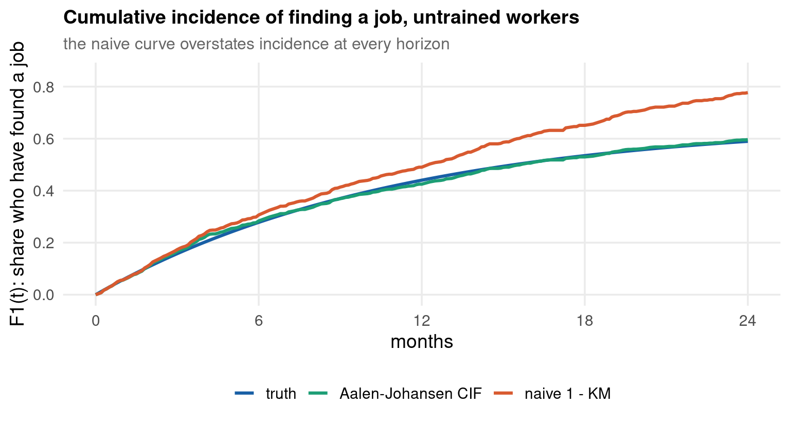
Code
import numpy as np
import pandas as pd
import matplotlib.pyplot as plt
from lifelines import KaplanMeierFitter

cr = pd.read_csv("../data/dsc-compete.csv")
s0 = cr[cr['train'] == 0]

# Aalen-Johansen: one pass over the ordered exit times
o = np.argsort(s0['time'].values)
t = s0['time'].values[o]
c = s0['cause'].values[o]
n = len(t)
S = 1.0
tt, ff = [0.0], [0.0]
for i in range(n):
    at_risk = n - i
    if c[i] == 1:
        ff.append(ff[-1] + S / at_risk)
        tt.append(t[i])
    if c[i] in (1, 2):
        S *= 1 - 1 / at_risk

km = KaplanMeierFitter().fit(s0['time'], s0['d1'])
g = np.arange(0, 24.01, 0.1)
truth = 0.06 / 0.09 * (1 - np.exp(-0.09 * g))
cif = np.interp(g, tt, ff)
naive = 1 - np.interp(g, km.survival_function_.index.values,
                      km.survival_function_.iloc[:, 0].values)

fig, ax = plt.subplots(figsize=(8, 4.3))
ax.plot(g, truth, color="#185FA5", lw=1.8, label="truth")
ax.plot(g, cif,   color="#1D9E75", lw=1.8, label="Aalen-Johansen CIF")
ax.plot(g, naive, color="#D85A30", lw=1.8, label="naive 1 - KM")
ax.text(0.03, 0.88, "at t = 24:  truth %.4f   CIF %.4f   naive %.4f"
        % (truth[-1], cif[-1], naive[-1]), transform=ax.transAxes,
        fontsize=10, color="#185FA5")
axopts = ax.set(xlim=(0, 24), ylim=(0, 0.85), xticks=range(0, 25, 6),
                yticks=np.arange(0, 0.81, 0.2), xlabel="months",
                ylabel="F1(t): share who have found a job",
                title="Cumulative incidence of finding a job, untrained workers")
ax.legend(frameon=False, loc="lower right")
plt.show()
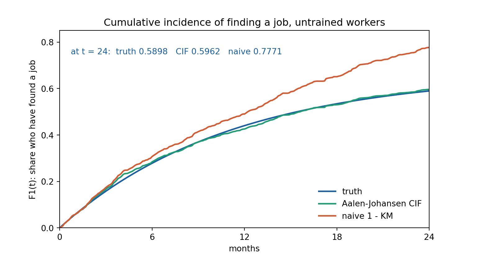
Code
quietly import delimited "../data/dsc-compete.csv", clear
quietly destring _all, replace

quietly stset time, failure(cause == 1)
quietly stcompet cif = ci, compet1(2) by(train)
quietly stset time, failure(d1 == 1)
quietly sts gen Snaive = s, by(train)
quietly gen naive = 1 - Snaive
quietly gen truth = (0.06/0.09) * (1 - exp(-0.09 * time))

* stcompet leaves cif missing on censored rows, which makes the plotted line
* drop to the axis and back at every one; carry the last value forward instead
sort train time
by train: gen double cifs = cif
by train: replace cifs = cifs[_n-1] if missing(cifs) & _n > 1
by train: replace cifs = max(cifs, cifs[_n-1]) if _n > 1

twoway (line truth time if train == 0, sort lcolor("24 95 165") lwidth(medthick))  ///
       (line cifs  time if train == 0, sort connect(stairstep)                      ///
            lcolor("29 158 117") lwidth(medthick))                                  ///
       (line naive time if train == 0, sort connect(stairstep)                      ///
            lcolor("216 90 48") lwidth(medthick)),                                  ///
    legend(order(1 "truth" 2 "Aalen-Johansen CIF" 3 "naive 1 - KM") rows(1)          ///
           size(small) position(6) ring(1) region(lstyle(none)))                                         ///
    xscale(range(0 24)) xlabel(0(6)24)                                               ///
    yscale(range(0 0.85)) ylabel(0(0.2)0.8)                                          ///
    xtitle("months") ytitle("F1(t): share who have found a job")                     ///
    title("Cumulative incidence of finding a job, untrained workers", size(medium))  ///
    subtitle("the naive curve overstates incidence at every horizon", size(small))   ///
    graphregion(color(white)) plotregion(color(white)) xsize(8) ysize(4.3)
graph export "../plots/dsc-p6-cif.png", replace width(1600)
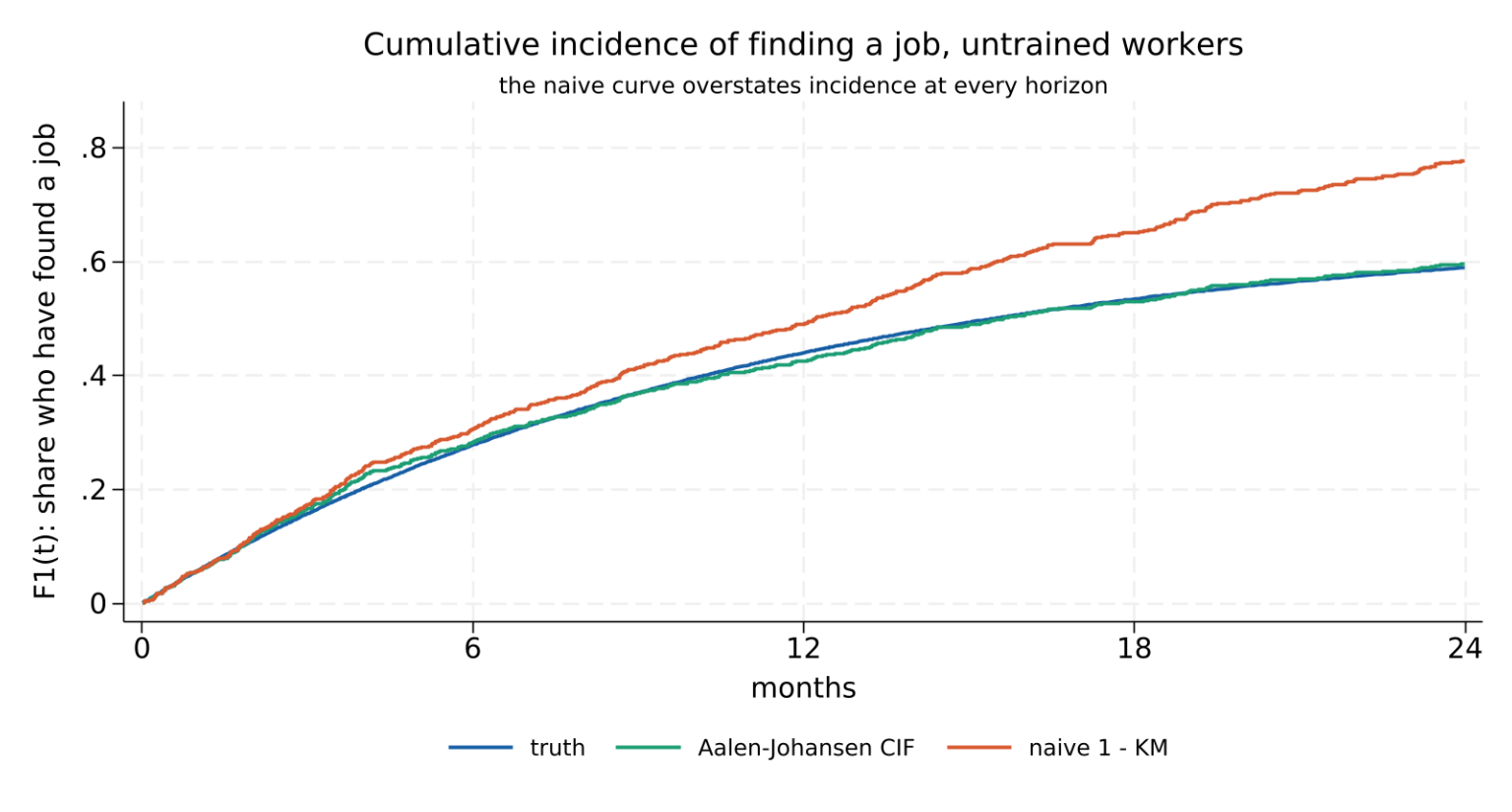
Trained workers reach \(F_1(24) = 0.7292\) against \(0.5962\) for the untrained — and their labour-force-exit incidence is lower, \(0.2031\) against \(0.2952\), because training raises one hazard and lowers the other. Both effects show up in the CIF; only one shows up in a cause-specific hazard ratio.

Aetiology or Prediction

Code
library(survival)
library(cmprsk)
cr <- read.csv("../data/dsc-compete.csv")

# cause-specific Cox: one model per cause, the other cause treated as
# censored FOR THE HAZARD only
c1 <- coxph(Surv(time, d1) ~ train, data = cr)
c2 <- coxph(Surv(time, d2) ~ train, data = cr)

# Fine-Gray subdistribution hazard for cause 1
fg <- crr(cr$time, cr$cause, cbind(train = cr$train), failcode = 1, cencode = 0)

out <- data.frame(
  model = c("cause-specific: job", "cause-specific: left LF",
            "Fine-Gray subdistribution: job"),
  coef  = round(c(coef(c1), coef(c2), fg$coef), 5),
  ratio = round(exp(c(coef(c1), coef(c2), fg$coef)), 4),
  se    = round(c(sqrt(diag(vcov(c1))), sqrt(diag(vcov(c2))),
                  sqrt(diag(fg$var))), 5),
  truth = c(0.40, -0.20, NA))
print(out, row.names = FALSE)
                          model     coef  ratio      se truth
            cause-specific: job  0.40470 1.4989 0.05531   0.4
        cause-specific: left LF -0.16408 0.8487 0.09182  -0.2
 Fine-Gray subdistribution: job  0.39623 1.4862 0.05531    NA
Code
import numpy as np
import pandas as pd
from lifelines import CoxPHFitter

cr = pd.read_csv("../data/dsc-compete.csv")

# A cause-specific Cox model is an ORDINARY Cox model on the cause indicator,
# so lifelines handles it natively - one fit per cause.
c1 = CoxPHFitter().fit(cr[['train', 'time', 'd1']], 'time', 'd1')
c2 = CoxPHFitter().fit(cr[['train', 'time', 'd2']], 'time', 'd2')

out = pd.DataFrame({
    'model': ["cause-specific: job", "cause-specific: left LF"],
    'coef': [round(c1.params_['train'], 5), round(c2.params_['train'], 5)],
    'ratio': [round(float(np.exp(c1.params_['train'])), 4),
              round(float(np.exp(c2.params_['train'])), 4)],
    'se': [round(c1.standard_errors_['train'], 5),
           round(c2.standard_errors_['train'], 5)],
    'truth': [0.40, -0.20]})

txt = (out.to_string(index=False) +
       "\n\nFine-Gray: NOT AVAILABLE in lifelines. The subdistribution risk set\n"
       "keeps cause-2 exits in place with time-dependent censoring weights,\n"
       "which no Python survival package currently implements. Use R's\n"
       "cmprsk::crr or Stata's stcrreg; both are shown alongside.")

import sys
nw = sys.stdout.write(txt + "\n")
                  model     coef  ratio      se  truth
    cause-specific: job  0.40470 1.4989 0.05531    0.4
cause-specific: left LF -0.16408 0.8487 0.09182   -0.2

Fine-Gray: NOT AVAILABLE in lifelines. The subdistribution risk set
keeps cause-2 exits in place with time-dependent censoring weights,
which no Python survival package currently implements. Use R's
cmprsk::crr or Stata's stcrreg; both are shown alongside.
Code
sys.stdout.flush()
Code
quietly import delimited "../data/dsc-compete.csv", clear
quietly destring _all, replace

quietly stset time, failure(d1 == 1)
quietly stcox train
display "cause-specific: job      b = " %8.5f _b[train] "  HR = " %6.4f exp(_b[train])

quietly stset time, failure(d2 == 1)
quietly stcox train
display "cause-specific: left LF  b = " %8.5f _b[train] "  HR = " %6.4f exp(_b[train])

* stcrreg: cause 1 is the failure, cause 2 the competing event
quietly stset time, failure(cause == 1)
stcrreg train, compete(cause == 2) nolog
cause-specific: job      b =  0.40470  HR = 1.4989


cause-specific: left LF  b = -0.16408  HR = 0.8487

        Failure _d: cause==1
  Analysis time _t: time

Competing-risks regression                        No. of obs      =      2,000
                                                  No. of subjects =      2,000
Failure event:   cause == 1                       No. failed      =      1,320
Competing event: cause == 2                       No. competing   =        502
                                                  No. censored    =        178

                                                  Wald chi2(1)    =      51.30
Log pseudolikelihood = -9421.5855                 Prob > chi2     =     0.0000

------------------------------------------------------------------------------
             |               Robust
          _t |        SHR   std. err.      z    P>|z|     [95% conf. interval]
-------------+----------------------------------------------------------------
       train |   1.486206   .0822162     7.16   0.000     1.333493    1.656407
------------------------------------------------------------------------------

The cause-specific models recover the truth: \(\hat\beta_1 = 0.40470\) against \(0.40\) and \(\hat\beta_2 = -0.16408\) against \(-0.20\), with standard errors \(0.055\) and \(0.092\). Training raises the job-finding rate by 50% and lowers the withdrawal rate by 15%.

The Fine–Gray subdistribution hazard ratio is \(1.4862\), very close to the cause-specific \(1.4989\) — because here both effects push \(F_1\) the same way.

They agree here by design, and will not in general. Reverse the second effect — make training also raise the withdrawal hazard — and the two diverge: the cause-specific ratio stays above 1 while the subdistribution ratio can fall below it, because more people are being removed from the pool who might have found jobs.

Rule of thumb: cause-specific for “why”, subdistribution for “how many”. If a paper reports only one, ask which question it was answering.

Discrete Time

recid records time in whole months: 552 events over 74 distinct values, up to 23 at once. Part 3 called these “ties” and applied Efron’s correction — a fix for an approximation problem in a continuous-time model.

But the ties are not an artefact of rounding an underlying continuous time. Or rather: they may be, and the distinction matters.

  • Grouped continuous time — the event happens at an exact instant, but only the month is recorded. Efron and Breslow are approximations to the truth.
  • Genuinely discrete time — decisions are made at discrete dates: benefit eligibility is reviewed monthly, contracts renew annually, harvests happen once a year. There is no underlying continuous clock.

In either case, when the number of intervals is small relative to the number of events, a discrete-time model is more honest and often easier.

Define the hazard as an actual probability, not a rate:

\[h_{it} = \Pr\big(T_i = t \mid T_i \ge t,\; \mathbf{x}_{it}\big) \in [0, 1]\]

Survival and the likelihood follow immediately:

\[S_{it} = \prod_{s=1}^{t}(1 - h_{is}), \qquad L = \prod_{i} \left[ \frac{h_{i t_i}}{1 - h_{i t_i}} \right]^{d_i} \prod_{s=1}^{t_i} (1 - h_{is})\]

Take logs and something remarkable appears:

\[\log L = \sum_{i}\sum_{s=1}^{t_i} \Big[ y_{is}\log h_{is} + (1 - y_{is})\log(1 - h_{is}) \Big], \qquad y_{is} = \mathbf{1}\{\text{event for } i \text{ at } s\}\]

That is exactly the log-likelihood of a binary regression on a dataset with one row per unit per period at risk. No special software is needed — the duration model is a panel binary model.

\[\textbf{logit:}\quad h_{it} = \frac{\exp(\alpha_t + \mathbf{x}_{it}'\boldsymbol{\beta})} {1 + \exp(\alpha_t + \mathbf{x}_{it}'\boldsymbol{\beta})}\]

\[\textbf{cloglog:}\quad h_{it} = 1 - \exp\!\big[-\exp(\alpha_t + \mathbf{x}_{it}'\boldsymbol{\beta})\big]\]

The complementary log-log is the one with a story. If the underlying process is continuous-time proportional hazards and you observe only the interval in which the event fell, then the interval hazard is exactly cloglog, with

\[\alpha_t = \log \int_{t-1}^{t} h_0(u)\,du\]

That is Prentice & Gloeckler (1978), and it makes \(\boldsymbol{\beta}\) in a cloglog discrete-time model the proportional-hazards coefficient — directly comparable to a Cox estimate, as the next slide shows.

Logit gives odds ratios rather than hazard ratios. When hazards are small the two coincide, which is why they agree so closely on this data.

\(\alpha_t\) is the discrete baseline hazard, and how you model it is a real choice:

Specification Cost Use when
a dummy per period most flexible; equals grouped Cox exactly few periods, many events each
polynomial in \(t\) parsimonious, smooth many periods
\(\log t\) one parameter, gives Weibull-like decline strong prior on shape
linear in \(t\) one parameter, Gompertz-like strong prior on shape

The code below uses \(\log t\): one parameter, and its coefficient reads as the Weibull shape minus one.

The Person-Period Expansion

One man becomes one row per month at risk. 1445 men become 80,013 rows, still carrying exactly 552 events.

Code
library(survival)
data("recid", package = "wooldridge")
recid <- transform(recid, fail = 1 - cens)

# survSplit cuts every spell at each month boundary
pp <- survSplit(Surv(durat, fail) ~ ., data = recid, cut = 1:80,
                episode = "period")
pp <- transform(pp, lper = log(period))

cat("person-period rows =", nrow(pp), "  events =", sum(pp$fail),
    "  men =", nrow(recid), "\n\n")

cll <- glm(fail ~ workprg + priors + tserved + black + married + lper,
           data = pp, family = binomial(link = "cloglog"))
lgt <- glm(fail ~ workprg + priors + tserved + black + married + lper,
           data = pp, family = binomial(link = "logit"))

print(round(coef(summary(cll)), 6))
cat("\ncloglog log-likelihood =", round(as.numeric(logLik(cll)), 4),
    "\nlogit   log-likelihood =", round(as.numeric(logLik(lgt)), 4), "\n")
person-period rows = 80013   events = 552   men = 1445 
             Estimate Std. Error    z value Pr(>|z|)
(Intercept) -4.345389   0.134851 -32.223682 0.000000
workprg     -0.033974   0.087849  -0.386735 0.698952
priors       0.050182   0.011427   4.391696 0.000011
tserved      0.008798   0.001467   5.995502 0.000000
black        0.374469   0.086046   4.351976 0.000013
married     -0.309298   0.106039  -2.916834 0.003536
lper        -0.321612   0.036299  -8.860106 0.000000

cloglog log-likelihood = -3215.106 
logit   log-likelihood = -3214.914 
Code
import numpy as np
import pandas as pd
import wooldridge as woo
import statsmodels.api as sm

rc = woo.data('recid').assign(fail=lambda d: 1 - d['cens'])
X = ['workprg', 'priors', 'tserved', 'black', 'married']

# one row per man per month at risk; the event flag is 1 only in the last
# month, and only for men who actually returned
rows = []
for r in rc.itertuples():
    T = int(r.durat)
    for k in range(1, T + 1):
        rows.append((r.workprg, r.priors, r.tserved, r.black, r.married,
                     k, int(k == T and r.fail == 1)))
pp = pd.DataFrame(rows, columns=X + ['period', 'fail'])
pp = pp.assign(lper=np.log(pp['period']))

Z = sm.add_constant(pp[X + ['lper']])
cll = sm.GLM(pp['fail'], Z,
             family=sm.families.Binomial(sm.families.links.CLogLog())).fit()
lgt = sm.GLM(pp['fail'], Z, family=sm.families.Binomial()).fit()

tab = pd.DataFrame({'coef': cll.params.round(6), 'se': cll.bse.round(6),
                    'z': (cll.params / cll.bse).round(4)})
txt = ("person-period rows = %d  events = %d  men = %d\n\n"
       % (len(pp), int(pp['fail'].sum()), len(rc))
       + tab.to_string()
       + "\n\ncloglog log-likelihood = %.4f\nlogit   log-likelihood = %.4f"
       % (cll.llf, lgt.llf))

import sys
nw = sys.stdout.write(txt + "\n")
person-period rows = 80013  events = 552  men = 1445

             coef        se        z
const   -4.345389  0.134851 -32.2237
workprg -0.033974  0.087849  -0.3867
priors   0.050182  0.011427   4.3917
tserved  0.008798  0.001467   5.9955
black    0.374469  0.086046   4.3520
married -0.309298  0.106039  -2.9168
lper    -0.321612  0.036299  -8.8601

cloglog log-likelihood = -3215.1065
logit   log-likelihood = -3214.9141
Code
sys.stdout.flush()
Code
quietly frause recid, clear
gen fail = 1 - cens
gen id = _n
* id() is REQUIRED before stsplit, and stsplit changes the time scale --
* a stale stset here gives plausible, wrong numbers with no error
stset durat, id(id) failure(fail == 1)
stsplit per, at(1(1)80)
replace per = per + 1
count
count if _d == 1
gen lper = ln(per)
glm _d workprg priors tserved black married lper, ///
    family(binomial) link(cloglog) nolog
quietly logit _d workprg priors tserved black married lper, nolog
display _newline "logit log-likelihood = " %10.4f e(ll)
Survival-time data settings

           ID variable: id
         Failure event: fail==1
Observed time interval: (durat[_n-1], durat]
     Exit on or before: failure

--------------------------------------------------------------------------
      1,445  total observations
          0  exclusions
--------------------------------------------------------------------------
      1,445  observations remaining, representing
      1,445  subjects
        552  failures in single-failure-per-subject data
     80,013  total analysis time at risk and under observation
                                                At risk from t =         0
                                     Earliest observed entry t =         0
                                          Last observed exit t =        81

(78,568 observations (episodes) created)

(80,013 real changes made)

  80,013

  552


Generalized linear models                         Number of obs   =     80,013
Optimization     : ML                             Residual df     =     80,006
                                                  Scale parameter =          1
Deviance         =  6430.212986                   (1/df) Deviance =   .0803716
Pearson          =  77769.66854                   (1/df) Pearson  =    .972048

Variance function: V(u) = u*(1-u)                 [Bernoulli]
Link function    : g(u) = ln(-ln(1-u))            [Complementary log–log]

                                                  AIC             =   .0805396
Log likelihood   = -3215.106493                   BIC             =  -896833.1

------------------------------------------------------------------------------
             |                 OIM
          _d | Coefficient  std. err.      z    P>|z|     [95% conf. interval]
-------------+----------------------------------------------------------------
     workprg |  -.0339742   .0878255    -0.39   0.699     -.206109    .1381607
      priors |   .0501817   .0114026     4.40   0.000      .027833    .0725305
     tserved |   .0087976    .001458     6.03   0.000     .0059401    .0116552
       black |    .374469   .0860368     4.35   0.000     .2058399     .543098
     married |   -.309298   .1060414    -2.92   0.004    -.5171353   -.1014606
        lper |  -.3216118   .0362411    -8.87   0.000    -.3926431   -.2505806
       _cons |  -4.345389   .1347115   -32.26   0.000    -4.609419   -4.081359
------------------------------------------------------------------------------


logit log-likelihood = -3214.9141

This is a panel binary model, and nothing more. The glm/logit calls above are the same commands the panel decks use for a binary outcome; the only duration content is in how the data were reshaped and in the \(\log t\) term. Everything those decks teach — clustered standard errors by id, random or fixed effects, marginal effects — applies here unchanged, and random effects on id is precisely the discrete-time version of Part 5’s frailty.

Cloglog Equals Grouped Cox

Code
data("recid", package = "wooldridge")
recid <- transform(recid, fail = 1 - cens)
pp <- survSplit(Surv(durat, fail) ~ ., data = recid, cut = 1:80,
                episode = "period")
pp <- transform(pp, lper = log(period))

cll <- glm(fail ~ workprg + priors + tserved + black + married + lper,
           data = pp, family = binomial(link = "cloglog"))
lgt <- glm(fail ~ workprg + priors + tserved + black + married + lper,
           data = pp, family = binomial(link = "logit"))
cx  <- coxph(Surv(durat, fail) ~ workprg + priors + tserved + black + married,
             data = recid, ties = "efron")

v <- c("workprg", "priors", "tserved", "black", "married")
cmp <- data.frame(cox = round(coef(cx)[v], 5),
                  cloglog = round(coef(cll)[v], 5),
                  logit = round(coef(lgt)[v], 5))
cmp <- transform(cmp, gap = round(cloglog - cox, 5))
print(cmp)

cat("\nlargest |cloglog - Cox| =", round(max(abs(cmp$gap)), 5),
    "\nlog(t) coefficient =", round(coef(cll)["lper"], 5),
    " -> implied Weibull shape p =", round(1 + coef(cll)["lper"], 5), "\n")
             cox  cloglog    logit      gap
workprg -0.03634 -0.03397 -0.03505  0.00237
priors   0.05035  0.05018  0.05077 -0.00017
tserved  0.00867  0.00880  0.00895  0.00013
black    0.36356  0.37447  0.37644  0.01091
married -0.31015 -0.30930 -0.31075  0.00085

largest |cloglog - Cox| = 0.01091 
log(t) coefficient = -0.32161  -> implied Weibull shape p = 0.67839 

The cloglog link inverts the continuous-time proportional hazard exactly. Over the interval \((t-1, t]\),

\[\Pr(T \le t \mid T > t-1, \mathbf{x}) = 1 - \exp\!\left[-\int_{t-1}^{t} h_0(u)\,du \cdot e^{\mathbf{x}'\boldsymbol{\beta}}\right] = 1 - \exp\!\big[-\exp(\alpha_t + \mathbf{x}'\boldsymbol{\beta})\big]\]

with \(\alpha_t = \log\int_{t-1}^{t} h_0(u)du\). The same \(\boldsymbol{\beta}\) appears in both, so the discrete-time cloglog coefficient is the proportional-hazards coefficient. Grouping the time axis costs information about when within the month, but changes no parameter.

The agreement here is close but not exact — the largest gap is \(0.011\) on black — for two reasons that are both about the baseline: the Cox model leaves \(h_0\) completely free, while the cloglog imposes \(\alpha_t = a + b\log t\); and Efron’s correction is an approximation where the cloglog is exact. Replace \(\log t\) with a full set of period dummies and the two coincide to numerical precision.

  • Time-varying covariates are trivial. The data are already one row per period; just vary the column. No counting-process syntax, no tmerge.
  • Frailty becomes a random effect. Part 5’s \(v_i\) is a random intercept on id, which every mixed-model routine fits — including in Python, where lifelines had nothing to offer.
  • Competing risks become a multinomial logit over the period’s outcome: no exit, exit by cause 1, exit by cause 2. The whole first half of this part collapses into a familiar estimator.
  • Institutional dates are dummies. A benefit-exhaustion spike at month 26 is one indicator variable, which no smooth parametric hazard can represent.

The cost is size. 1445 men became 80,013 rows here; a daily panel over ten years would be unusable, and that is when continuous-time methods earn their keep. Under a few hundred periods, discrete time is usually the more flexible and more transparent choice — and it puts the whole toolkit of panel binary models at your disposal.

Part 7 — Count Data

Poisson, overdispersion, and what to do about zeros

Counts: Why \(\exp(\mathbf{x}'\boldsymbol{\beta})\)

Part 1 opened with “how long until”. This part answers “how many”:

  • arrests per year, per man
  • patents per firm, per year
  • doctor visits, strikes, bank failures, trade flows between country pairs

The outcome \(y \in \{0, 1, 2, \dots\}\) is a non-negative integer, usually small, usually with a big pile at zero. crime1 (Wooldridge Chapter 17) has 2725 men, mean arrests \(0.4044\) — and 72.3% of them have none.

 arrests  men share
       0 1970 72.29
       1  559 20.51
       2  121  4.44
       3   42  1.54
       4   12  0.44
       5   13  0.48
       6    4  0.15

mean = 0.4044   variance = 0.73801   ratio = 1.8249 

Linear regression on a count runs into the same wall as linear regression on a duration: \(\mathbf{x}'\boldsymbol{\beta}\) can be negative and \(\mathbb{E}[y]\) cannot. The fix is the same:

\[\mathbb{E}[y \mid \mathbf{x}] = \mu(\mathbf{x}) = \exp(\mathbf{x}'\boldsymbol{\beta}) > 0\]

Three things follow, and they are the whole reason this is the standard choice.

Coefficients are semi-elasticities.

\[\frac{\partial \log \mathbb{E}[y \mid \mathbf{x}]}{\partial x_j} = \beta_j\]

so \(\beta_j\) is the proportional change in the expected count per unit of \(x_j\) — the same reading as a log-linear regression, but without needing \(\log y\) and therefore without the zeros problem.

Zeros are not a nuisance. \(\log(y + 1)\) regressions, the common alternative, depend on the arbitrary constant and estimate nothing interpretable. With 72% of this sample at zero, that matters.

It connects to the first half of this deck. A Poisson count over an interval of length \(t\) with rate \(\mu\) is exactly the number of events of a Poisson process whose hazard is \(\mu\). Duration and counts are two views of the same process — which is why Part 6’s person-period logit sits between them.

The companion deck Computational Trade Models derives Poisson pseudo-maximum likelihood as the gravity estimator — Santos Silva & Tenreyro’s argument about log-linearised gravity, the zeros problem in bilateral trade, separation, and the PML family.

This part derives the same robustness result as a count model, and then goes where the trade deck does not: formal overdispersion testing, the negative binomial and its two variants, zero-inflation versus hurdles, truncation, and fixed-effects Poisson for panels.

If you have read that deck, skip to the overdispersion slide. If you have not, nothing here depends on it.

Poisson and the QMLE Result

Assume \(y_i \mid \mathbf{x}_i \sim \text{Poisson}(\mu_i)\), \(\mu_i = \exp(\mathbf{x}_i'\boldsymbol{\beta})\):

\[\log L = \sum_{i=1}^{n} \big[\, y_i \mathbf{x}_i'\boldsymbol{\beta} - \exp(\mathbf{x}_i'\boldsymbol{\beta}) - \log y_i! \,\big]\]

The score is the familiar residual-times-regressor form,

\[\frac{\partial \log L}{\partial \boldsymbol{\beta}} = \sum_{i=1}^{n} \big(y_i - \mu_i\big)\,\mathbf{x}_i = \mathbf{0}\]

and the Hessian \(-\sum_i \mu_i \mathbf{x}_i\mathbf{x}_i'\) is negative definite for any \(\mathbf{x}\) of full rank. The log-likelihood is globally concave: one maximum, no starting values to worry about, convergence in a handful of Newton steps.

The score also forces \(\sum_i \hat\mu_i = \sum_i y_i\) when a constant is included — mean fitted equals mean observed, exactly, which is the check the code slide prints.

The Poisson distribution imposes equidispersion, \(\mathrm{Var}[y \mid \mathbf{x}] = \mathbb{E}[y \mid \mathbf{x}]\), and real count data essentially never satisfy it. crime1 has a variance-to-mean ratio of \(1.825\).

Gouriéroux, Monfort & Trognon (1984) showed this does not matter for consistency. The score is a moment condition requiring only

\[\mathbb{E}\big[\,y_i \mid \mathbf{x}_i\,\big] = \exp(\mathbf{x}_i'\boldsymbol{\beta})\]

Nothing else about the distribution enters. So:

\[\boxed{\;\hat{\boldsymbol{\beta}}_{\text{Poisson}} \text{ is consistent whenever the CONDITIONAL MEAN is right,}\;}\]

no matter what the variance, the higher moments, or the share of zeros look like. The Poisson MLE is really a quasi-MLE — a GMM estimator wearing a likelihood’s clothes.

The standard errors are not robust, and they are wrong in the dangerous direction. The information-matrix equality fails under overdispersion, so the default MLE errors are too small. Use the sandwich:

\[\widehat{\mathrm{Var}}[\hat{\boldsymbol{\beta}}] = \Big(\textstyle\sum_i \hat\mu_i \mathbf{x}_i\mathbf{x}_i'\Big)^{-1} \Big(\textstyle\sum_i (y_i - \hat\mu_i)^2 \mathbf{x}_i\mathbf{x}_i'\Big) \Big(\textstyle\sum_i \hat\mu_i \mathbf{x}_i\mathbf{x}_i'\Big)^{-1}\]

On crime1 the robust errors are 1.08 to 1.39 times the MLE ones. Reporting the default would overstate every \(t\)-statistic by up to 39%.

The practical consequence is a hierarchy that surprises people:

  • Poisson with robust standard errors — consistent under a correct mean, whatever the variance. Safe.
  • Negative binomial — a full likelihood. If its variance function is wrong, \(\hat{\boldsymbol{\beta}}\) is inconsistent, not merely inefficient.
  • Zero-inflated / hurdle — more structure again, more ways to be wrong.

So the extra models below are not simply “better”. They buy efficiency and a richer description of the distribution, and they buy it by assuming more. Poisson QMLE remains the estimator to beat, and the one to report alongside anything fancier.

Poisson on crime1

Wooldridge’s Example 17.3: arrests in 1986 explained by the conviction rate, sentence length, time in prison, employment and demographics.

Code
library(sandwich)
library(lmtest)
data("crime1", package = "wooldridge")

ps <- glm(narr86 ~ pcnv + avgsen + tottime + ptime86 + qemp86 + inc86 +
            black + hispan + born60,
          data = crime1, family = poisson)

# robust (sandwich) standard errors are the default worth reporting
print(coeftest(ps, vcov = sandwich))

cat("\nlog-likelihood =", round(as.numeric(logLik(ps)), 4),
    "  n =", nrow(crime1), "\n")
cat("mean fitted =", round(mean(fitted(ps)), 6),
    "  mean observed =", round(mean(crime1$narr86), 6),
    "   (the score forces these equal)\n")
cat("robust / MLE se ratio: min",
    round(min(sqrt(diag(sandwich(ps))) / sqrt(diag(vcov(ps)))), 4),
    " max", round(max(sqrt(diag(sandwich(ps))) / sqrt(diag(vcov(ps)))), 4), "\n")

z test of coefficients:

              Estimate Std. Error z value  Pr(>|z|)    
(Intercept) -0.5995888  0.0893299 -6.7121 1.919e-11 ***
pcnv        -0.4015713  0.1011433 -3.9703 7.178e-05 ***
avgsen      -0.0237723  0.0236035 -1.0072    0.3139    
tottime      0.0244904  0.0204985  1.1947    0.2322    
ptime86     -0.0985584  0.0222994 -4.4198 9.880e-06 ***
qemp86      -0.0380187  0.0341446 -1.1135    0.2655    
inc86       -0.0080807  0.0012274 -6.5838 4.586e-11 ***
black        0.6608376  0.0994389  6.6457 3.019e-11 ***
hispan       0.4998133  0.0923704  5.4110 6.269e-08 ***
born60      -0.0510286  0.0811254 -0.6290    0.5293    
---
Signif. codes:  0 '***' 0.001 '**' 0.01 '*' 0.05 '.' 0.1 ' ' 1

log-likelihood = -2248.761   n = 2725 
mean fitted = 0.404404   mean observed = 0.404404    (the score forces these equal)
robust / MLE se ratio: min 1.0775  max 1.3897 
Code
import numpy as np
import wooldridge as woo
import statsmodels.api as sm

cr = woo.data('crime1')
xn = ['pcnv', 'avgsen', 'tottime', 'ptime86', 'qemp86', 'inc86',
      'black', 'hispan', 'born60']
X = sm.add_constant(cr[xn])
y = cr['narr86']

ps  = sm.Poisson(y, X).fit(disp=0)                    # MLE errors
psr = sm.Poisson(y, X).fit(disp=0, cov_type='HC0')    # sandwich errors

txt = (str(psr.summary().tables[1]) +
       "\n\nlog-likelihood = %.4f   n = %d" % (psr.llf, int(psr.nobs)) +
       "\nmean fitted = %.6f   mean observed = %.6f   (the score forces these equal)"
       % (psr.predict().mean(), y.mean()) +
       "\nrobust / MLE se ratio: min %.4f  max %.4f"
       % ((psr.bse / ps.bse).min(), (psr.bse / ps.bse).max()))

import sys
nw = sys.stdout.write(txt + "\n")
==============================================================================
                 coef    std err          z      P>|z|      [0.025      0.975]
------------------------------------------------------------------------------
const         -0.5996      0.089     -6.712      0.000      -0.775      -0.425
pcnv          -0.4016      0.101     -3.970      0.000      -0.600      -0.203
avgsen        -0.0238      0.024     -1.007      0.314      -0.070       0.022
tottime        0.0245      0.020      1.195      0.232      -0.016       0.065
ptime86       -0.0986      0.022     -4.420      0.000      -0.142      -0.055
qemp86        -0.0380      0.034     -1.113      0.266      -0.105       0.029
inc86         -0.0081      0.001     -6.584      0.000      -0.010      -0.006
black          0.6608      0.099      6.646      0.000       0.466       0.856
hispan         0.4998      0.092      5.411      0.000       0.319       0.681
born60        -0.0510      0.081     -0.629      0.529      -0.210       0.108
==============================================================================

log-likelihood = -2248.7611   n = 2725
mean fitted = 0.404404   mean observed = 0.404404   (the score forces these equal)
robust / MLE se ratio: min 1.0775  max 1.3897
Code
sys.stdout.flush()
Code
quietly frause crime1, clear
poisson narr86 pcnv avgsen tottime ptime86 qemp86 inc86 black hispan born60, ///
    vce(robust) nolog
quietly predict double mu, n
quietly summarize mu
display "mean fitted   = " %9.6f r(mean)
quietly summarize narr86
display "mean observed = " %9.6f r(mean)
Poisson regression                                      Number of obs =  2,725
                                                        Wald chi2(9)  = 246.22
                                                        Prob > chi2   = 0.0000
Log pseudolikelihood = -2248.7611                       Pseudo R2     = 0.0791

------------------------------------------------------------------------------
             |               Robust
      narr86 | Coefficient  std. err.      z    P>|z|     [95% conf. interval]
-------------+----------------------------------------------------------------
        pcnv |  -.4015713   .1011619    -3.97   0.000    -.5998449   -.2032976
      avgsen |  -.0237723   .0236078    -1.01   0.314    -.0700427    .0224981
     tottime |   .0244904   .0205023     1.19   0.232    -.0156934    .0646741
     ptime86 |  -.0985584   .0223035    -4.42   0.000    -.1422724   -.0548445
      qemp86 |  -.0380187   .0341509    -1.11   0.266    -.1049532    .0289158
       inc86 |  -.0080807   .0012276    -6.58   0.000    -.0104867   -.0056747
       black |   .6608376   .0994572     6.64   0.000     .4659051      .85577
      hispan |   .4998133   .0923874     5.41   0.000     .3187374    .6808892
      born60 |  -.0510286   .0811403    -0.63   0.529    -.2100606    .1080034
       _cons |  -.5995888   .0893463    -6.71   0.000    -.7747044   -.4244732
------------------------------------------------------------------------------


mean fitted   =  0.404404


mean observed =  0.404404

Parity. All three give a log-likelihood of \(-2248.7611\) and identical coefficients: pcnv \(-0.401571\), ptime86 \(-0.098558\), black \(0.660838\), hispan \(0.499813\). Mean fitted equals mean observed at \(0.404404\) in all three.

Robust standard errors match to four decimals — pcnv is \(0.10114\) in R and Python against \(0.10116\) in Stata, the difference being Stata’s \(n/(n-1)\) finite-sample scaling.

Reading the Coefficients

Semi-elasticity — the coefficient itself. \(\beta_{\text{pcnv}} = -0.4016\): a one-unit rise in the conviction proportion (from 0 to 1) lowers the expected arrest count by about 40 log points.

Incidence-rate ratio\(\exp(\beta)\), the multiplicative effect:

\[\mathrm{IRR}_j = \frac{\mathbb{E}[y \mid x_j + 1]}{\mathbb{E}[y \mid x_j]} = e^{\beta_j}\]

Average marginal effect — in counts, not ratios:

\[\mathrm{AME}_j = \frac{1}{n}\sum_i \frac{\partial \mu_i}{\partial x_j} = \beta_j \cdot \frac{1}{n}\sum_i \hat\mu_i = \beta_j \cdot \bar{y}\]

The last equality is a small gift of the Poisson score: because mean fitted equals mean observed, the AME is just the coefficient times the sample mean of \(y\).

            coef     IRR pct_change      AME
pcnv    -0.40157 0.66927     -33.07 -0.16240
avgsen  -0.02377 0.97651      -2.35 -0.00961
tottime  0.02449 1.02479       2.48  0.00990
ptime86 -0.09856 0.90614      -9.39 -0.03986
qemp86  -0.03802 0.96269      -3.73 -0.01537
inc86   -0.00808 0.99195      -0.80 -0.00327
black    0.66084 1.93641      93.64  0.26725
hispan   0.49981 1.64841      64.84  0.20213
born60  -0.05103 0.95025      -4.97 -0.02064
  • black: \(\mathrm{IRR} = 1.936\), a 94% higher expected arrest count, or \(+0.267\) arrests per man per year at the sample mean
  • pcnv: moving the conviction proportion from 0 to 1 cuts expected arrests 33%, or \(-0.162\) arrests
  • ptime86: each month in prison during 1986 lowers expected arrests 9.4% — mechanically, since a man in prison cannot be arrested outside

Do not report a percentage change of \(100\beta\) when \(\beta\) is large. For black, \(\beta = 0.6608\) is not “a 66% increase” — the exact figure is \(e^{0.6608} - 1 = 93.6\%\). The approximation \(e^\beta - 1 \approx \beta\) is fine below about \(0.1\) and badly wrong above \(0.5\).

Not causal. pcnv is the man’s own past conviction rate, jointly determined with his criminal behaviour. Wooldridge presents this as a descriptive specification, and so should you.

Not a probability. \(\mathrm{IRR} = 1.936\) is about expected counts. The probability of any arrest changes by a different, smaller factor, and if that is the question, a binary model answers it directly.

Not stable across models. The negative binomial two slides on gives pcnv \(-0.477\) against Poisson’s \(-0.402\) — a 19% difference from a change in the assumed variance, which under a correct mean specification should not have moved the estimate at all. That gap is a specification signal worth taking seriously.

Overdispersion

Poisson imposes \(\mathrm{Var}[y \mid \mathbf{x}] = \mu\). The alternative worth testing against nests it:

\[\mathrm{Var}[y \mid \mathbf{x}] = \mu + \alpha\, g(\mu), \qquad H_0: \alpha = 0\]

with \(g(\mu) = \mu^2\) giving NB2 and \(g(\mu) = \mu\) giving NB1.

Cameron & Trivedi (1990) turn this into an auxiliary OLS regression. Under \(H_0\), \(\mathbb{E}[(y-\mu)^2 - y \mid \mathbf{x}] = 0\), so with \(\hat\mu\) from the Poisson fit, regress

\[\frac{(y_i - \hat\mu_i)^2 - y_i}{\hat\mu_i} = \alpha \cdot \frac{g(\hat\mu_i)}{\hat\mu_i} + \text{error}\]

and read off the \(t\)-statistic on \(\alpha\). No constant. It is a one-sided test — underdispersion is possible but rare — and it needs no distributional assumption beyond the mean.

Pearson statistic over degrees of freedom:

\[\frac{1}{n-k}\sum_i \frac{(y_i - \hat\mu_i)^2}{\hat\mu_i}\]

should be near 1. On crime1 it is \(1.5168\).

Raw variance-to-mean ratio: \(0.7380 / 0.4044 = 1.825\). Crude, because it ignores covariates — some of that spread is explained variation — but a useful first look.

Overdispersion has causes, and they suggest different fixes.

  • unobserved heterogeneity — individuals differ in ways you do not observe, so the marginal distribution mixes many Poissons. This is exactly Part 5’s frailty: a gamma-mixed Poisson is the negative binomial.
  • true contagion — one arrest raises the chance of the next; the events are not independent
  • excess zeros — a subpopulation with no risk at all; the zeros inflate the variance
  • omitted variables or a wrong functional form — the mean is misspecified, and then Poisson QMLE is inconsistent too

The first three leave the conditional mean intact, so Poisson-with-robust-errors survives. The fourth does not, and no amount of variance modelling repairs it.

Negative Binomial

Let the Poisson mean carry an unobserved multiplicative term, \(\mathbb{E}[y \mid \mathbf{x}, v] = \mu v\) with \(v \sim \text{Gamma}\), mean 1, variance \(\alpha\). Integrating \(v\) out gives a closed form:

\[\Pr(y \mid \mathbf{x}) = \frac{\Gamma(y + 1/\alpha)}{\Gamma(1/\alpha)\,\Gamma(y+1)} \left(\frac{1/\alpha}{1/\alpha + \mu}\right)^{1/\alpha} \left(\frac{\mu}{1/\alpha + \mu}\right)^{y}\]

\[\mathbb{E}[y \mid \mathbf{x}] = \mu, \qquad \mathrm{Var}[y \mid \mathbf{x}] = \mu + \alpha\mu^2\]

This is Part 5’s mixed proportional hazard, in count form. The same gamma mixture, the same closed-form Laplace transform, the same parameter \(\alpha\) measuring unobserved heterogeneity. Duration and counts really are one subject.

Variance Dispersion as \(\mu\) grows Software
NB1 \(\mu + \alpha\mu = (1+\alpha)\mu\) constant ratio Stata nbreg, dispersion(constant)
NB2 \(\mu + \alpha\mu^2\) grows with \(\mu\) the default everywhere

NB2 is the default because it arises from the gamma mixture above and because its score has the same GMM interpretation as Poisson’s. NB1 is a linear variance function — the “quasi-Poisson” of the GLM literature, up to how the errors are computed.

The choice is not cosmetic. NB2 is a genuine likelihood, so \(\hat{\beta}\) is inconsistent if the variance function is wrong, unlike Poisson QMLE. That is the trade: efficiency under a correct variance, inconsistency under an incorrect one. Reporting Poisson-with-robust-errors beside the NB is not padding; it is the check.

Code
library(MASS)
data("crime1", package = "wooldridge")
f <- narr86 ~ pcnv + avgsen + tottime + ptime86 + qemp86 + inc86 +
  black + hispan + born60

ps <- glm(f, data = crime1, family = poisson)
nb <- glm.nb(f, data = crime1)

# Cameron-Trivedi regression-based test, both variance forms
mu <- fitted(ps)
y  <- crime1$narr86
z  <- ((y - mu)^2 - y) / mu
ct2 <- lm(z ~ mu - 1)            # NB2: Var = mu + alpha * mu^2
ct1 <- lm(z ~ 1)                 # NB1: Var = mu + alpha * mu

cat("Cameron-Trivedi test\n")
cat("  NB2 form: alpha =", round(coef(ct2), 6),
    "  t =", round(summary(ct2)$coefficients[3], 4), "\n")
cat("  NB1 form: alpha =", round(coef(ct1), 6),
    "  t =", round(summary(ct1)$coefficients[3], 4), "\n")
cat("  Pearson chi2 / df =",
    round(sum(residuals(ps, "pearson")^2) / ps$df.residual, 5), "\n\n")

cat("NB2 alpha =", round(1 / nb$theta, 6),
    "  (theta =", round(nb$theta, 5), ")\n")
cat("LR test Poisson vs NB2: chi2 =",
    round(2 * (as.numeric(logLik(nb)) - as.numeric(logLik(ps))), 4),
    "  (boundary: halve the p-value)\n\n")
print(round(summary(nb)$coefficients, 5))
Cameron-Trivedi test
  NB2 form: alpha = 1.245731   t = 4.8183 
  NB1 form: alpha = 0.500054   t = 4.1003 
  Pearson chi2 / df = 1.51679 
NB2 alpha = 0.928773   (theta = 1.07669 )
LR test Poisson vs NB2: chi2 = 182.2662   (boundary: halve the p-value)
            Estimate Std. Error  z value Pr(>|z|)
(Intercept) -0.56374    0.08130 -6.93435  0.00000
pcnv        -0.47710    0.10108 -4.72021  0.00000
avgsen      -0.01734    0.02554 -0.67888  0.49721
tottime      0.01974    0.01943  1.01593  0.30966
ptime86     -0.10740    0.02433 -4.41399  0.00001
qemp86      -0.05049    0.03478 -1.45168  0.14659
inc86       -0.00771    0.00115 -6.69751  0.00000
black        0.65604    0.09244  7.09675  0.00000
hispan       0.50485    0.08922  5.65853  0.00000
born60      -0.04641    0.07747 -0.59910  0.54910
Code
import numpy as np
import pandas as pd
import wooldridge as woo
import statsmodels.api as sm

cr = woo.data('crime1')
xn = ['pcnv', 'avgsen', 'tottime', 'ptime86', 'qemp86', 'inc86',
      'black', 'hispan', 'born60']
X = sm.add_constant(cr[xn])
y = cr['narr86']

ps = sm.Poisson(y, X).fit(disp=0)
nb = sm.NegativeBinomial(y, X).fit(disp=0)

# Cameron-Trivedi auxiliary regression
mu = ps.predict()
z = ((y - mu) ** 2 - y) / mu
ct2 = sm.OLS(z, mu).fit()                      # NB2 form, no constant
ct1 = sm.OLS(z, np.ones(len(z))).fit()         # NB1 form
pearson = np.sum((y - mu) ** 2 / mu) / (len(y) - X.shape[1])

tab = pd.DataFrame({'coef': nb.params.round(5), 'se': nb.bse.round(5),
                    'z': nb.tvalues.round(4), 'p': nb.pvalues.round(5)})

txt = ("Cameron-Trivedi test\n"
       "  NB2 form: alpha = %.6f   t = %.4f\n"
       "  NB1 form: alpha = %.6f   t = %.4f\n"
       "  Pearson chi2 / df = %.5f\n\n"
       % (ct2.params.iloc[0], ct2.tvalues.iloc[0],
          ct1.params[0], ct1.tvalues[0], pearson)
       + "NB2 alpha = %.6f\n" % nb.params['alpha']
       + "LR test Poisson vs NB2: chi2 = %.4f   (boundary: halve the p-value)\n\n"
       % (2 * (nb.llf - ps.llf))
       + tab.to_string())

import sys
nw = sys.stdout.write(txt + "\n")
Cameron-Trivedi test
  NB2 form: alpha = 1.245731   t = 4.8183
  NB1 form: alpha = 0.500054   t = 4.1003
  Pearson chi2 / df = 1.51679

NB2 alpha = 0.928776
LR test Poisson vs NB2: chi2 = 182.2662   (boundary: halve the p-value)

            coef       se       z        p
const   -0.56376  0.08271 -6.8159  0.00000
pcnv    -0.47713  0.10333 -4.6175  0.00000
avgsen  -0.01734  0.02612 -0.6639  0.50678
tottime  0.01974  0.01923  1.0263  0.30473
ptime86 -0.10740  0.02507 -4.2833  0.00002
qemp86  -0.05048  0.03519 -1.4348  0.15135
inc86   -0.00771  0.00115 -6.7274  0.00000
black    0.65603  0.09236  7.1030  0.00000
hispan   0.50488  0.08957  5.6369  0.00000
born60  -0.04637  0.07764 -0.5973  0.55034
alpha    0.92878  0.10937  8.4917  0.00000
Code
sys.stdout.flush()
Code
quietly frause crime1, clear
quietly poisson narr86 pcnv avgsen tottime ptime86 qemp86 inc86 black hispan born60
estat gof
predict double mu, n
gen double ctz = ((narr86 - mu)^2 - narr86) / mu
* Cameron-Trivedi auxiliary regression, NB2 form (no constant)
regress ctz mu, noconstant
* nbreg is NB2; the reported LR test of alpha = 0 is Poisson vs NB
nbreg narr86 pcnv avgsen tottime ptime86 qemp86 inc86 black hispan born60, nolog
         Deviance goodness-of-fit =  2822.185
         Prob > chi2(2715)        =    0.0742

         Pearson goodness-of-fit  =   4118.08
         Prob > chi2(2715)        =    0.0000

      Source |       SS           df       MS      Number of obs   =     2,725
-------------+----------------------------------   F(1, 2724)      =     23.22
       Model |  938.750805         1  938.750805   Prob > F        =    0.0000
    Residual |  110145.253     2,724  40.4351149   R-squared       =    0.0085
-------------+----------------------------------   Adj R-squared   =    0.0081
       Total |  111084.004     2,725   40.764772   Root MSE        =    6.3589

------------------------------------------------------------------------------
         ctz | Coefficient  Std. err.      t    P>|t|     [95% conf. interval]
-------------+----------------------------------------------------------------
          mu |   1.245731   .2585404     4.82   0.000     .7387757    1.752686
------------------------------------------------------------------------------


Negative binomial regression                            Number of obs =  2,725
                                                        LR chi2(9)    = 266.12
Dispersion: mean                                        Prob > chi2   = 0.0000
Log likelihood = -2157.628                              Pseudo R2     = 0.0581

------------------------------------------------------------------------------
      narr86 | Coefficient  Std. err.      z    P>|z|     [95% conf. interval]
-------------+----------------------------------------------------------------
        pcnv |  -.4770963   .1033295    -4.62   0.000    -.6796183   -.2745743
      avgsen |  -.0173385   .0261171    -0.66   0.507    -.0685272    .0338501
     tottime |   .0197394   .0192325     1.03   0.305    -.0179557    .0574344
     ptime86 |  -.1073997    .025074    -4.28   0.000    -.1565439   -.0582555
      qemp86 |  -.0504884   .0351857    -1.43   0.151    -.1194511    .0184743
       inc86 |  -.0077126   .0011465    -6.73   0.000    -.0099596   -.0054656
       black |   .6560406   .0923594     7.10   0.000     .4750195    .8370617
      hispan |   .5048465   .0895663     5.64   0.000     .3292998    .6803932
      born60 |   -.046412   .0776384    -0.60   0.550    -.1985804    .1057564
       _cons |  -.5637368   .0827121    -6.82   0.000    -.7258495   -.4016242
-------------+----------------------------------------------------------------
    /lnalpha |  -.0738912   .1177617                     -.3046999    .1569175
-------------+----------------------------------------------------------------
       alpha |   .9287728   .1093739                      .7373446    1.169899
------------------------------------------------------------------------------
LR test of alpha=0: chibar2(01) = 182.27               Prob >= chibar2 = 0.000

Overdispersion is decisive and identically measured everywhere. The Cameron–Trivedi NB2 statistic is \(\hat\alpha = 1.245731\) with \(t = 4.82\); the NB1 form gives \(\hat\alpha = 0.50005\) with \(t = 4.10\); Pearson \(\chi^2/\text{df} = 1.51679\). The NB2 likelihood gives \(\hat\alpha = 0.928773\) and a likelihood ratio of \(182.27\) against Poisson.

Notice what changed and what did not. Every sign is the same and every conclusion survives, but pcnv moves from \(-0.4016\) to \(-0.4771\) and avgsen’s \(t\)-statistic falls below 1. Under a correctly specified mean these should not have moved — the NB is only meant to be more efficient. That they did is a hint the mean itself is imperfect, which is what the zeros slide takes up.

Excess Zeros

crime1 has 1970 zeros out of 2725 — 72.3%. Two models explain a pile of zeros, and they mean different things.

Zero-inflated. There are two latent groups. A share \(\pi(\mathbf{z})\) are never at risk and always produce zero; the rest follow a count model that can itself produce a zero:

\[\Pr(y = 0) = \pi + (1 - \pi) f(0), \qquad \Pr(y = k) = (1 - \pi) f(k)\;\; \text{for } k \ge 1\]

The story: some men never commit crimes at all. Their zero is structural. Everyone else’s zero is a matter of luck.

Hurdle. Everyone faces the same two-stage decision. First cross a hurdle (offend at all), then choose how often, from a zero-truncated distribution:

\[\Pr(y = 0) = 1 - \pi(\mathbf{z}), \qquad \Pr(y = k) = \pi(\mathbf{z}) \frac{f(k)}{1 - f(0)}\;\; \text{for } k \ge 1\]

The story: participation and intensity are separate decisions. No zero is structural; a zero simply means the hurdle was not crossed.

Choose on the economics, not on the fit. Zero-inflation says some units cannot have the outcome; a hurdle says all could but did not. In demand for medical care the hurdle is natural — everyone could visit a doctor. In counts of children born to women who are physiologically unable to conceive, zero-inflation is natural. For arrests either story is arguable, which is exactly why the tests below cannot settle it.

The Vuong (1989) test for non-nested models is the traditional way to choose zero-inflated over plain. It is not valid for this comparison, and the reason is simple: the standard count model is a boundary case of the zero-inflated one (\(\pi = 0\)), so the models are nested, and Vuong’s non-nested asymptotics do not apply.

Wilson (2015) works through the consequences: the test over-rejects, and it systematically favours the zero-inflated model. Its behaviour on crime1 is a textbook illustration, on the next slide.

What to do instead

  • compare predicted zero counts against the observed number
  • use AIC or BIC across the whole family, which at least penalises parameters consistently
  • decide the structure from economics and use fit only to choose within it
  • test overdispersion first — very often the “excess” zeros disappear once the variance is free

Zero-Inflated and Hurdle

Code
library(pscl)
library(MASS)
data("crime1", package = "wooldridge")

f  <- narr86 ~ pcnv + avgsen + tottime + ptime86 + qemp86 + inc86 +
  black + hispan + born60
fz <- narr86 ~ pcnv + avgsen + tottime + ptime86 + qemp86 + inc86 +
  black + hispan + born60 | pcnv + inc86 + black + hispan

ps <- glm(f, data = crime1, family = poisson)
nb <- glm.nb(f, data = crime1)
zi <- zeroinfl(fz, data = crime1, dist = "negbin")
hd <- hurdle(fz, data = crime1, dist = "poisson")

fit <- data.frame(
  model = c("Poisson", "NB2", "hurdle Poisson", "ZINB"),
  logL  = round(c(logLik(ps), logLik(nb), logLik(hd), logLik(zi)), 4),
  k     = c(attr(logLik(ps), "df"), attr(logLik(nb), "df"),
            attr(logLik(hd), "df"), attr(logLik(zi), "df")),
  AIC   = round(c(AIC(ps), AIC(nb), AIC(hd), AIC(zi)), 3),
  pred0 = round(c(sum(dpois(0, fitted(ps))),
                  sum(dnbinom(0, mu = fitted(nb), size = nb$theta)),
                  sum(predict(hd, type = "prob")[, 1]),
                  sum(predict(zi, type = "prob")[, 1])), 1))
print(fit, row.names = FALSE)
cat("\nobserved zeros =", sum(crime1$narr86 == 0), "of", nrow(crime1), "\n\n")

cat("ZINB inflation equation:\n")
print(round(summary(zi)$coefficients$zero, 5))
cat("\nVuong, NB2 versus ZINB:\n")
vuong(nb, zi)
          model      logL  k      AIC  pred0
        Poisson -2248.761 10 4517.522 1868.9
            NB2 -2157.628 11 4337.256 1987.1
 hurdle Poisson -2164.061 15 4358.121 1970.0
           ZINB -2129.193 16 4290.386 1993.2

observed zeros = 1970 of 2725 
ZINB inflation equation:
            Estimate Std. Error  z value Pr(>|z|)
(Intercept) -4.19558    1.17306 -3.57662  0.00035
pcnv         5.12351    1.12403  4.55818  0.00001
inc86        0.00273    0.00341  0.79895  0.42432
black       -0.91814    0.47502 -1.93283  0.05326
hispan      -0.80309    0.41711 -1.92536  0.05418

Vuong, NB2 versus ZINB:
Vuong Non-Nested Hypothesis Test-Statistic: 
(test-statistic is asymptotically distributed N(0,1) under the
 null that the models are indistinguishible)
-------------------------------------------------------------
              Vuong z-statistic             H_A   p-value
Raw                   -3.694863 model2 > model1 0.0001100
AIC-corrected         -3.045162 model2 > model1 0.0011628
BIC-corrected         -1.125222 model2 > model1 0.1302476
Code
import numpy as np
import pandas as pd
import wooldridge as woo
import statsmodels.api as sm
from scipy.optimize import minimize
from scipy.special import gammaln
from statsmodels.discrete.truncated_model import TruncatedLFPoisson

cr = woo.data('crime1')
xn = ['pcnv', 'avgsen', 'tottime', 'ptime86', 'qemp86', 'inc86',
      'black', 'hispan', 'born60']
X = sm.add_constant(cr[xn]).values
Z = sm.add_constant(cr[['pcnv', 'inc86', 'black', 'hispan']]).values
y = cr['narr86'].values.astype(float)

ps = sm.Poisson(y, X).fit(disp=0)
nb = sm.NegativeBinomial(y, X).fit(disp=0)

# statsmodels' ZINB will not converge here, so the NB2 zero-inflated
# log-likelihood is coded directly. th = (gamma, beta, log alpha).
def nll_zinb(th):
    g, b, a = th[:Z.shape[1]], th[Z.shape[1]:-1], np.exp(th[-1])
    w = 1 / (1 + np.exp(-(Z @ g)))
    mu = np.exp(X @ b)
    r, p = 1 / a, (1 / a) / ((1 / a) + np.exp(X @ b))
    lnb = (gammaln(y + r) - gammaln(r) - gammaln(y + 1)
           + r * np.log(p) + y * np.log1p(-p))
    return -np.sum(np.where(y == 0, np.log(w + (1 - w) * np.exp(r * np.log(p))),
                            np.log1p(-w) + lnb))

start = np.r_[np.zeros(Z.shape[1]), nb.params[:-1], np.log(nb.params[-1])]
zi = minimize(nll_zinb, start, method='BFGS',
              options={'maxiter': 20000, 'gtol': 1e-8})

# hurdle-Poisson = logit for y>0 plus a zero-truncated Poisson on y>0.
# TruncatedLFPoisson needs method='newton'; bfgs stalls far from the optimum.
lg = sm.Logit((y > 0).astype(float), Z).fit(disp=0)
tp = TruncatedLFPoisson(y[y > 0], X[y > 0]).fit(method='newton', disp=0)
hd_llf = lg.llf + tp.llf

def aic(ll, k):
    return -2 * ll + 2 * k

mu_nb = nb.predict()
a_nb = nb.params[-1]
pred0 = [np.exp(-ps.predict()).sum(),
         ((1 / a_nb) / ((1 / a_nb) + mu_nb)) ** (1 / a_nb),
         (1 - lg.predict()).sum(), np.nan]
pred0[1] = pred0[1].sum()
w_zi = 1 / (1 + np.exp(-(Z @ zi.x[:Z.shape[1]])))
mu_zi = np.exp(X @ zi.x[Z.shape[1]:-1])
r_zi = 1 / np.exp(zi.x[-1])
pred0[3] = (w_zi + (1 - w_zi) * (r_zi / (r_zi + mu_zi)) ** r_zi).sum()

fit = pd.DataFrame({
    'model': ["Poisson", "NB2", "hurdle Poisson", "ZINB"],
    'logL': np.round([ps.llf, nb.llf, hd_llf, -zi.fun], 4),
    'k': [X.shape[1], X.shape[1] + 1, X.shape[1] + Z.shape[1],
          X.shape[1] + Z.shape[1] + 1],
    'pred0': np.round(pred0, 1)})
fit['AIC'] = np.round(aic(fit['logL'], fit['k']), 3)

infl = pd.Series(np.round(zi.x[:Z.shape[1]], 5),
                 index=["(Intercept)", "pcnv", "inc86", "black", "hispan"])

txt = (fit[['model', 'logL', 'k', 'AIC', 'pred0']].to_string(index=False) +
       "\n\nobserved zeros = %d of %d" % ((y == 0).sum(), len(y)) +
       "\n\nZINB inflation equation:\n" + infl.to_string())

import sys
nw = sys.stdout.write(txt + "\n")
         model       logL  k      AIC  pred0
       Poisson -2248.7611 10 4517.522 1868.9
           NB2 -2157.6280 11 4337.256 1987.1
hurdle Poisson -2164.0606 15 4358.121 1970.0
          ZINB -2129.1929 16 4290.386 1993.1

observed zeros = 1970 of 2725

ZINB inflation equation:
(Intercept)   -4.19242
pcnv           5.11889
inc86          0.00274
black         -0.91774
hispan        -0.80092
Code
sys.stdout.flush()
Code
quietly frause crime1, clear
local xs pcnv avgsen tottime ptime86 qemp86 inc86 black hispan born60

quietly poisson narr86 `xs', nolog
scalar ll_p = e(ll)
quietly nbreg narr86 `xs', nolog
scalar ll_nb = e(ll)
zinb narr86 `xs', inflate(pcnv inc86 black hispan) nolog
scalar ll_zi = e(ll)

* Stata has no count hurdle command: build it from its two parts.
* The log-likelihood is additive, which is what makes the hurdle a hurdle.
gen byte pos = narr86 > 0
quietly logit pos pcnv inc86 black hispan, nolog
scalar ll_h1 = e(ll)
quietly tpoisson narr86 `xs' if narr86 > 0, ll(0) nolog
scalar ll_h2 = e(ll)

display _newline "model" _col(20) "logL" _col(34) "k" _col(44) "AIC"
display "Poisson"        _col(16) %10.4f ll_p  _col(32) 10 _col(38) %10.3f -2*ll_p  + 2*10
display "NB2"            _col(16) %10.4f ll_nb _col(32) 11 _col(38) %10.3f -2*ll_nb + 2*11
display "hurdle Poisson" _col(16) %10.4f ll_h1 + ll_h2 _col(32) 15 ///
        _col(38) %10.3f -2*(ll_h1 + ll_h2) + 2*15
display "ZINB"           _col(16) %10.4f ll_zi _col(32) 16 _col(38) %10.3f -2*ll_zi + 2*16
count if narr86 == 0
Zero-inflated negative binomial regression              Number of obs =  2,725
Inflation model: logit                                  Nonzero obs   =    755
                                                        Zero obs      =  1,970
                                                        LR chi2(9)    = 139.49
Log likelihood = -2129.193                              Prob > chi2   = 0.0000

------------------------------------------------------------------------------
      narr86 | Coefficient  Std. err.      z    P>|z|     [95% conf. interval]
-------------+----------------------------------------------------------------
narr86       |
        pcnv |   .4740472   .1722211     2.75   0.006     .1365001    .8115942
      avgsen |  -.0234887   .0259339    -0.91   0.365    -.0743181    .0273408
     tottime |   .0201619   .0192363     1.05   0.295    -.0175406    .0578644
     ptime86 |  -.1143656   .0248898    -4.59   0.000    -.1631487   -.0655824
      qemp86 |  -.0457834   .0347353    -1.32   0.187    -.1138634    .0222966
       inc86 |  -.0068388    .001226    -5.58   0.000    -.0092416   -.0044359
       black |   .5193863   .0988316     5.26   0.000     .3256799    .7130928
      hispan |   .3182879   .1003748     3.17   0.002      .121557    .5150189
      born60 |  -.0848224   .0768727    -1.10   0.270    -.2354901    .0658453
       _cons |  -.5909178   .0869906    -6.79   0.000    -.7614161   -.4204194
-------------+----------------------------------------------------------------
inflate      |
        pcnv |   5.118878   1.121093     4.57   0.000     2.921577     7.31618
       inc86 |    .002741   .0034058     0.80   0.421    -.0039343    .0094163
       black |  -.9177416   .4750198    -1.93   0.053    -1.848763    .0132802
      hispan |  -.8009181   .4168195    -1.92   0.055    -1.617869     .016033
       _cons |  -4.192408    1.17018    -3.58   0.000    -6.485918   -1.898898
-------------+----------------------------------------------------------------
    /lnalpha |  -.4843505   .1787473    -2.71   0.007    -.8346889   -.1340122
-------------+----------------------------------------------------------------
       alpha |   .6160972   .1101257                      .4340095    .8745794
------------------------------------------------------------------------------


model              logL          k         AIC

Poisson        -2248.7611      10      4517.522

NB2            -2157.6280      11      4337.256

hurdle Poisson -2164.0606      15      4358.121

ZINB           -2129.1929      16      4290.386

  1,970

The Vuong test does exactly what Wilson (2015) predicts. Comparing NB2 with ZINB, the raw statistic is \(-3.695\) (\(p = 0.00011\)) — apparently decisive for zero-inflation. The AIC-corrected version is \(-3.045\) (\(p = 0.0012\)). The BIC-corrected version is \(-1.125\) (\(p = 0.130\)) — no evidence at all.

Three versions of one test on one dataset, spanning “highly significant” to “nothing there”. Any of the three could be quoted, and papers quote whichever they find. This is the concrete reason not to select zero-inflation by Vuong.

The predicted-zero column settles the substance without any test. Poisson predicts \(1868.9\) zeros against \(1970\) observed — a genuine shortfall of about \(100\). But the negative binomial already predicts \(1987.1\), slightly over the observed count, and ZINB’s \(1993.2\) adds nothing.

crime1 does not have a zeros problem. It has an overdispersion problem. Once the variance is free to exceed the mean, the “excess” zeros are explained. The AIC ordering — ZINB \(4290.4\), NB2 \(4337.3\), hurdle-Poisson \(4358.1\), Poisson \(4517.5\) — puts ZINB narrowly ahead, but the ZINB spends five extra parameters to gain \(47\) points over NB2 while predicting almost the same number of zeros, and its inflation equation is driven almost entirely by pcnv (\(5.12\), \(z = 4.56\)), which is mechanically related to having been arrested.

The defensible report is negative binomial, with Poisson-plus-robust-errors alongside, and a sentence saying that zero-inflation was tried and added nothing beyond what free dispersion already delivered.

Truncation, Censoring and Panels

Part 1’s distinction returns unchanged. A truncated count sample excludes units by their outcome, so the likelihood must be conditioned on selection:

\[\Pr(y \mid \mathbf{x},\, y > 0) = \frac{f(y \mid \mathbf{x})}{1 - f(0 \mid \mathbf{x})}\]

This is the count component of the hurdle, standing alone. It is the right model whenever the sample only contains positives:

  • on-site sampling — surveying visitors at a park about how often they visit; non-visitors are unreachable by construction
  • administrative case files — only people who filed at least one claim appear
  • firm registries of exporters, which by definition record firms with positive trade

Ignoring truncation biases the constant sharply and attenuates the slopes. Estimating a plain Poisson on the 755 men with at least one arrest would be exactly this mistake.

Censored counts are the top-coded case: the questionnaire offers “5 or more”. Stata’s cpoisson handles it; the likelihood replaces \(f(y)\) with \(\Pr(y \ge 5)\) at the cap.

Code
data("crime1", package = "wooldridge")

# the 755 men with at least one arrest, as if they were the whole sample
pos <- subset(crime1, narr86 > 0)

# VGAM is called through its namespace: attaching it masks several
# survival and stats functions used elsewhere in this deck
zt <- VGAM::vglm(narr86 ~ pcnv + avgsen + tottime + ptime86 + qemp86 + inc86 +
                   black + hispan + born60,
                 family = VGAM::pospoisson(), data = pos)

cat("n =", nrow(pos), "  log-likelihood =", round(VGAM::logLik(zt), 4), "\n\n")
print(round(VGAM::coef(zt), 5))

# what ignoring the truncation would give
naive <- glm(narr86 ~ pcnv + avgsen + tottime + ptime86 + qemp86 + inc86 +
               black + hispan + born60, data = pos, family = poisson)
cat("\nintercept: truncated", round(VGAM::coef(zt)[1], 5),
    " vs naive Poisson", round(coef(naive)[1], 5), "\n")
cat("pcnv:      truncated", round(VGAM::coef(zt)[2], 5),
    " vs naive Poisson", round(coef(naive)[2], 5), "\n")
n = 755   log-likelihood = -667.1471 
(Intercept)        pcnv      avgsen     tottime     ptime86      qemp86 
   -0.11831     0.66099    -0.06802     0.05394     0.03226    -0.19398 
      inc86       black      hispan      born60 
   -0.00706     0.38532     0.31829    -0.25383 

intercept: truncated -0.11831  vs naive Poisson 0.44592 
pcnv:      truncated 0.66099  vs naive Poisson 0.23515 
Code
import numpy as np
import pandas as pd
import wooldridge as woo
import statsmodels.api as sm
from statsmodels.discrete.truncated_model import TruncatedLFPoisson

cr = woo.data('crime1')
xn = ['pcnv', 'avgsen', 'tottime', 'ptime86', 'qemp86', 'inc86',
      'black', 'hispan', 'born60']
pos = cr[cr['narr86'] > 0]
X = sm.add_constant(pos[xn])
y = pos['narr86']

# method='newton' is required: the default BFGS stalls well short of the optimum
zt = TruncatedLFPoisson(y, X).fit(method='newton', disp=0)
naive = sm.Poisson(y, X).fit(disp=0)

txt = ("n = %d  log-likelihood = %.4f\n\n" % (len(pos), zt.llf)
       + zt.params.round(5).to_string()
       + "\n\nintercept: truncated %.5f  vs naive Poisson %.5f"
       % (zt.params['const'], naive.params['const'])
       + "\npcnv:      truncated %.5f  vs naive Poisson %.5f"
       % (zt.params['pcnv'], naive.params['pcnv']))

import sys
nw = sys.stdout.write(txt + "\n")
n = 755  log-likelihood = -667.1471

const     -0.11831
pcnv       0.66099
avgsen    -0.06802
tottime    0.05394
ptime86    0.03226
qemp86    -0.19398
inc86     -0.00706
black      0.38532
hispan     0.31829
born60    -0.25383

intercept: truncated -0.11831  vs naive Poisson 0.44592
pcnv:      truncated 0.66099  vs naive Poisson 0.23515
Code
sys.stdout.flush()
Code
quietly frause crime1, clear
local xs pcnv avgsen tottime ptime86 qemp86 inc86 black hispan born60
* ll(0) means "the sample is truncated below at 0", i.e. only positives observed
tpoisson narr86 `xs' if narr86 > 0, ll(0) nolog
quietly poisson narr86 `xs' if narr86 > 0, nolog
display _newline "naive Poisson on the same subsample: _cons = " %8.5f _b[_cons] ///
        "   pcnv = " %8.5f _b[pcnv]
Truncated Poisson regression                    Number of obs     =        755
Limits:  lower =          0                     LR chi2(9)        =     321.47
         upper =       +inf                     Prob > chi2       =     0.0000
Log likelihood = -667.14707                     Pseudo R2         =     0.1942

------------------------------------------------------------------------------
      narr86 | Coefficient  Std. err.      z    P>|z|     [95% conf. interval]
-------------+----------------------------------------------------------------
        pcnv |   .6609906   .1524163     4.34   0.000     .3622602    .9597209
      avgsen |  -.0680206   .0350312    -1.94   0.052    -.1366805    .0006392
     tottime |   .0539391   .0212121     2.54   0.011     .0123641    .0955141
     ptime86 |   .0322599    .039933     0.81   0.419    -.0460073    .1105271
      qemp86 |  -.1939824   .0576499    -3.36   0.001    -.3069742   -.0809906
       inc86 |  -.0070621    .002863    -2.47   0.014    -.0126735   -.0014507
       black |    .385323   .1223199     3.15   0.002     .1455804    .6250656
      hispan |   .3182917   .1284574     2.48   0.013     .0665197    .5700636
      born60 |  -.2538259    .110494    -2.30   0.022    -.4703902   -.0372617
       _cons |  -.1183123   .1194994    -0.99   0.322    -.3525268    .1159022
------------------------------------------------------------------------------


naive Poisson on the same subsample: _cons =  0.44592   pcnv =  0.23515

The panel case deserves its own note, because the result is unusually strong. With a multiplicative unit effect,

\[\mathbb{E}[y_{it} \mid \mathbf{x}_i, c_i] = c_i \exp(\mathbf{x}_{it}'\boldsymbol{\beta})\]

Hausman, Hall & Griliches (1984) showed that conditioning on \(\sum_t y_{it}\) eliminates \(c_i\) exactly, leaving a multinomial conditional likelihood in \(\boldsymbol{\beta}\) alone. There is no incidental-parameters problem — unlike fixed-effects logit or probit, where short panels bias everything.

Wooldridge (1999) went further: the conditional score is a valid moment condition under the mean assumption alone, so fixed-effects Poisson with clustered standard errors is consistent even when \(y\) is overdispersed, serially correlated, or not a count at all.

Command
Stata xtpoisson y x, fe vce(robust), or ppmlhdfe for many fixed effects
R fixest::fepois(y ~ x | id + t)
Python pyfixest.fepois()

That last robustness result is why the gravity literature estimates trade flows — continuous, non-negative, heavily skewed, full of zeros — with a Poisson command. The companion deck Computational Trade Models develops it at length with ppmlhdfe; nothing is repeated here beyond the pointer.

The truncated fit reproduces to four decimals in all three languages — \(\log L = -667.1471\) on 755 men — and the contrast with the naive Poisson on the same subsample is stark: the intercept moves from \(-0.11831\) to \(0.44592\) and pcnv from \(0.66099\) to \(0.23515\). Fitting an untruncated model to a truncated sample understates the slope by 64%, and gets the intercept wrong by more than half a log point.

Part 8 — Practice, Exercises, Reading

What to check, what to report, and what to read next

Model-Selection Checklist

1. Draw the data. Kaplan–Meier first, Nelson–Aalen second. The shape of \(\hat H\) tells you whether a monotone family is defensible before any likelihood is maximised.

2. Count the events, not the observations. Precision comes from events. 1445 men with 552 events supports roughly 55 covariates by the ten-events-per-parameter rule of thumb; the same 1445 men with 40 events supports four.

3. Establish where censoring comes from. Administrative end-of-study is benign. Attrition, competing exits and stock sampling are not, and each has a different fix — Part 6, Part 6, and Part 1’s enter() respectively.

4. Ask whether the spell can end in more than one way. If yes, and the ways differ economically, Part 6 is not optional.

5. Decide what you must report. A hazard ratio needs a Cox model. A median duration or a ten-year forecast needs a parametric one. Let the deliverable choose the estimator.

Data shape Estimator
one binary covariate, description Kaplan–Meier + log-rank
several covariates, hazard ratios wanted Cox, efron ties, cox.zph afterwards
PH rejected for one covariate stratify it, or interact it with time
extrapolation, medians, \(\mathbb{E}[T]\) wanted parametric AFT; race the families on \(\Delta\)AIC
time recorded in coarse intervals, few of them discrete-time cloglog on person-periods
several exit routes cause-specific Cox per cause and the CIFs
the shape of duration dependence is the question MPH with frailty — and read Part 5 twice
repeated spells per unit shared frailty, or cluster on the unit
outcome is “how many” Poisson QMLE with robust errors, then test dispersion
  • Test proportional hazards, and say which time transform you used
  • Test overdispersion before choosing any count model beyond Poisson
  • Compare predicted to observed — survival at fixed horizons; the number of zeros for counts
  • Refit the headline in a second package. Every number in this deck was verified across R, Python and Stata, and doing so found a Breslow-versus-Efron default, a non-converging truncated NB, and a statsmodels optimiser that stops short with no error
  • Report the sample: \(n\), events, censored, and the longest observed spell

Common Pitfalls

1. A stale stset. stset is stateful and every st* command inherits it silently. Part 6’s stsplit changes the time scale; forgetting to re-declare gives plausible, wrong numbers and no error. Re-stset at the top of any chunk that changes the time axis.

2. The censoring indicator built differently in different languages. recid codes cens = 1 for still free — the opposite of an event. Three languages, three chances to get the polarity wrong, and every downstream curve looks reasonable. Part 2 prints 1445 / 552 / 893 in all three tabs for exactly this reason.

3. Ties left on the default. stcox uses Breslow; coxph and lifelines use Efron. With 7.5 events per event time the coefficients differ in the third decimal and a cross-package comparison looks like a data bug.

4. Proportional hazards assumed rather than tested. One hazard ratio for a covariate whose effect halves after six months is an average over an unstated weighting. Test it; if it fails, the failure is a result.

5. Hazard ratios read as duration ratios. \(\mathrm{HR} = 1.5\) is not “spells are 50% shorter”. Under a Weibull with shape \(p\) the duration ratio is \(\mathrm{HR}^{-1/p}\), which on recid turns \(1.5451\) into \(0.583\).

6. A competing exit coded as censoring. The naive Kaplan–Meier overstated cumulative incidence by 30% on data where the truth was known. No warning is issued, and the curve looks fine.

7. The Vuong test used to justify zero-inflation. Its three variants on crime1 gave \(p = 0.0001\), \(p = 0.0012\) and \(p = 0.13\). Wilson (2015) explains why none of them is valid for a nested boundary comparison.

These produce no error, no warning, and a clean-looking table.

  • Left-truncation without enter() — a stock sample analysed as a flow sample. The hazard comes out too low and duration dependence too negative, which is indistinguishable from frailty
  • Extrapolating a parametric fit far past the data — the Weibull median of 462 months from 81 months of data, with a confidence interval that measures only parameter uncertainty
  • A dispersion parameter on a boundary — the negative binomial hurdle that “converged” in R with \(\hat\alpha = 22.9\) while Stata refused
  • A ConvergenceWarning in a long logstatsmodels’ truncated Poisson stopping at \(-788.57\) instead of \(-667.15\)
  • Frailty variance estimated from the tail you barely observe\(\hat\theta\) is identified by long durations, which heavy censoring removes

Reporting negative duration dependence from a model without frailty. This deck’s central demonstration: on data built with a constant hazard, a Weibull recovered \(\hat p = 0.7434\) with \(z = -5.6\); on recid, adding one frailty parameter moved \(\hat p\) from \(0.8059\) to \(1.7079\) — from significantly negative to significantly positive duration dependence.

The observed hazard declines. Whether the individual hazard declines is a separate question, and the data cannot answer it without an assumption you must state.

What to Report

The sample. \(n\), number of events, number censored, source of censoring, longest observed spell. Four integers and a sentence.

The estimator. Model, tie-handling method, and — for parametric fits — the family and why. “Cox proportional hazards, Efron ties” is complete; “a survival model” is not.

The coefficients. Hazard ratios with standard errors and intervals. If the audience thinks in durations, add the implied duration ratio and say how you converted.

The assumption tests. The proportional-hazards test with its time transform, and what you did if it failed.

The picture. Predicted survival at two or three interpretable covariate profiles beats a table of ratios for every audience outside a seminar.

The horizon. State the last observed event time, and mark anything beyond it as extrapolation.

The distribution. Mean, variance, share of zeros, and the maximum. Three numbers that tell a reader immediately whether Poisson is plausible.

The estimator and its errors. “Poisson with robust standard errors” as the baseline. If you report only a negative binomial, you are asking readers to believe a variance function they cannot check.

The dispersion test. Cameron–Trivedi \(\hat\alpha\) and its \(t\), or Pearson \(\chi^2/\text{df}\). Do this before reaching for zero-inflation.

Predicted versus observed zeros. One line, and it settles most zero-inflation arguments — on crime1, \(1970\) observed against \(1868.9\) from Poisson and \(1987.1\) from the negative binomial.

Effects in two units. The IRR and the average marginal effect. Ratios travel badly outside the seminar; counts do not.

  • “We find negative duration dependence” — from a model without frailty. Write “the observed hazard declines” and say what would be needed to go further.
  • “Mean duration is 55.4 months” — when 62% of spells are censored, that averages durations with lower bounds.
  • “The hazard ratio is 1.5, so spells are a third shorter” — different units.
  • “The Vuong test favours zero-inflation” — the test is invalid for this comparison.
  • “Standard errors are clustered, so group correlation is handled” — clustering fixes variances, not the point estimates a shared-frailty model would change.
  • “The median predicted duration is 462 months” — from 81 months of data, without saying so.

Variations and Extensions

Interval-censored data. Annual waves tell you the event happened somewhere in a year. Stata’s stintreg fits parametric models directly; R has icenReg. Treating the interview date as the event date is a real, common bias.

Cure models. A fraction of the population will never experience the event — firms that never exit, patients cured. The survivor function has a plateau:

\[S(t) = \pi + (1 - \pi)\,S_0(t)\]

This is Part 7’s zero-inflation, in duration form. R’s flexsurvcure, Stata’s strsmix.

Multi-state models. Beyond competing risks: units move between several states and back — employed, unemployed, out of the labour force. R’s msm and mstate; the whole apparatus generalises the Part 6 machinery.

Survival forests and ML. randomForestSRC and scikit-survival fit hazards without a functional form and handle interactions automatically. They give predictions, not coefficients, and no assumption test — a different tool for a different job. The companion deck Machine Learning: Trees and Ensembles covers the underlying estimators.

Structural duration models. Rust’s optimal-stopping framework treats the exit decision as a dynamic programme; the hazard emerges from the value function rather than being specified. The companion deck Structural Estimation in Econometrics develops it. The trade is explicitness against portability: a structural model answers counterfactual questions this deck cannot touch, and only under its own assumptions.

Extension Buys Costs
interval censoring the correct likelihood for wave data a parametric family, usually
cure model a plateau in \(S(t)\) one more mixing parameter, weakly identified
multi-state transitions in both directions many more parameters; needs a large panel
survival forest prediction, interactions for free no coefficients, no assumption test
structural counterfactuals a full behavioural model, and its assumptions

Each row is the same trade this deck has made at every step: Part 3 bought freedom over \(h_0\) by assuming proportionality, Part 4 bought extrapolation by assuming a family, Part 5 bought the true shape by assuming a frailty distribution. There is no free flexibility.

Endogeneity

Every estimate above is conditional on observables, and workprg in recid is the standing example: men select into the prison work programme, so its hazard ratio of \(1.088\) describes who participates as much as what participation does.

The Part 2 log-rank found nothing (\(\chi^2 = 0.289\)), the Part 3 Cox found nothing (\(p = 0.35\)), the Part 4 AFT found nothing (\(p = 0.32\)) — and none of those agreements is evidence about the programme’s effect. They agree because they are the same conditional association computed three ways.

Instrumental variables for counts. ivpoisson fits both the GMM and control function versions:

ivpoisson gmm y x1 (x2 = z1 z2)          // additive or multiplicative errors
ivpoisson cfunction y x1 (x2 = z1 z2)    // control function

R’s ivtools, or hand-coded GMM on the moment \(\mathbb{E}[\mathbf{z}(y - e^{\mathbf{x}'\boldsymbol{\beta}})] = 0\).

Control functions for duration. Estimate the first stage, take the residual, and enter it as an extra regressor in the hazard. Consistent under a specific error structure, and the standard errors need a bootstrap.

Timing-of-events. Abbring & van den Berg (2003) is the identification result economists should know: with an MPH structure and a treatment that arrives at a random time, the treatment effect on the hazard is identified from the timing alone — no exclusion restriction needed. The assumption doing the work is the proportional-hazards structure, which is why Part 3’s test matters beyond goodness-of-fit. 10.1111/1468-0262.00456

Nothing in this deck makes workprg causal. The honest description of Parts 2–5 is that they describe conditional associations in a well-specified way, which is a prerequisite for a causal claim and not a substitute for one.

Exercises — Estimation

Use recid, crime1 and fertil2 — all three load natively in R, Python and Stata — plus the two simulated files where indicated. Do each in at least two languages and check that the numbers agree before interpreting them.

  1. Reproduce the Part 2 Kaplan–Meier on recid and add a stratification by black. Report \(\hat S(12)\), \(\hat S(36)\) and \(\hat S(60)\) in each group, and the log-rank statistic. Does the median exist in either group?
  2. Fit the Part 3 Cox model with all three tie-handling methods. Tabulate the ten coefficients side by side and report the largest absolute difference between Efron and Breslow. Then drop tserved and priors and re-check: does the ties problem get better or worse, and why?
  3. Fit Weibull, log-normal, log-logistic and Gompertz to recid. Report \(\Delta\)AIC against the best. Then refit on the subsample black == 0 and report whether the ranking changes.
  4. Using the Weibull AFT fit, compute the predicted median duration and its 95% interval for a man aged 25 (age = 300), 12 years of education, no priors, married, with one year served. Do the same for the same man unmarried. Report both, and state the last observed event time.
  5. On dsc-frailty.csv, fit the gamma-frailty MPH from a starting value of \(\theta = 5\) rather than \(\theta = 1\). Does it reach the same optimum? Now fit with \(\theta\) fixed at \(0.5, 1, 2, 3, 4\) and plot the profile log-likelihood against \(\theta\). How flat is it?
  6. On dsc-compete.csv, estimate the cumulative incidence of cause 2 (leaving the labour force) for both training groups. Compare with the closed-form truth \(F_2(t) = \frac{h_2}{h_1+h_2}(1 - e^{-(h_1+h_2)t})\). Then compute a naive Kaplan–Meier for cause 2 and quantify its overstatement.
  7. Build the person-period expansion of recid and fit the discrete-time cloglog with a full set of period dummies instead of \(\log t\). Compare the coefficients with the Cox model. How much closer do they get than the \(\log t\) version’s largest gap of \(0.011\)?
  8. Fit Poisson and negative binomial to fertil2, explaining ceb (children ever born) with age, educ, electric, urban and protestant. Report the Cameron–Trivedi statistic, the share of zeros, and the predicted versus observed zero count for both models.
  9. Take the 755 men in crime1 with at least one arrest and fit both a plain and a zero-truncated Poisson. Reproduce the 64% attenuation in pcnv, then explain in two sentences why the naive fit is biased toward zero.
  10. Simulate 2000 spells from a Weibull with \(p = 1.4\) and no frailty, seed 14159, censoring at the 60th percentile. Fit with and without gamma frailty. Does the frailty model correctly report \(\hat\theta \approx 0\), and what does its likelihood-ratio test say?

Exercises — Testing and Specification

  1. Run cox.zph / estat phtest on the Part 3 model under all four time transforms (identity, rank, KM, log). Tabulate the global statistic and the priors statistic for each. Which covariate is most sensitive to the choice, and what does that tell you about when its effect changes?
  2. For the covariate that comes closest to failing the PH test, fit a model interacting it with \(\log t\). Report the interaction, its \(z\), and the likelihood-ratio test against the constant-effect model. Then plot the implied hazard ratio against \(t\).
  3. Split recid at month 24 and fit separate Cox models on \([0, 24)\) and \([24, 81]\) using the counting-process form. Compare the coefficient on priors across the two windows. Is the difference significant, and does it agree with what the Schoenfeld test said?
  4. Test the exponential restriction \(p = 1\) on recid three ways: the Wald test on \(\log \hat p\), a likelihood-ratio test against the exponential, and the Cameron–Trivedi-style comparison of the Nelson–Aalen curve with a straight line. Do they agree?
  5. On dsc-frailty.csv, run the Part 4 family horse race without frailty. Which family wins, and what shape does it attribute to a hazard that is truly constant? Explain the result using the observed-hazard formula \(\bar h = h_0 e^{\mathbf{x}\beta} / (1 + \theta H_0 e^{\mathbf{x}\beta})\).
  6. Refit the recid MPH of Part 5 with inverse-Gaussian frailty instead of gamma (streg ..., frailty(invgaussian)). Report \(\hat p\) and \(\hat\theta\). Does the sign of duration dependence survive the change of frailty family? Write the sentence you would put in a paper.
  7. Fit the Fine–Gray model on dsc-compete.csv after modifying the data so that train raises the labour-force-exit hazard (multiply cause-2 times for trained workers by \(e^{-0.5}\) before censoring). Do the cause-specific and subdistribution hazard ratios now disagree in sign? Explain which answers which question.
  8. On crime1, compute all three Vuong variants for NB2 against ZINB, then repeat on a bootstrap sample of size 1000 drawn with replacement, 200 times. What fraction of the replications would lead you to choose zero-inflation at the 5% level under each variant?
  9. Test overdispersion in crime1 using both the NB1 and NB2 forms of the Cameron–Trivedi regression. Then fit gnbreg (NB1) and nbreg (NB2) and compare AIC. Does the test pick the same variant the AIC does?
  10. Take the discrete-time model of Part 6 and add a random intercept on the man (xtlogit, re or lme4::glmer). Report the estimated variance of the random effect and compare it with the \(\hat\theta = 5.99\) from the continuous-time gamma-frailty fit. Should they be equal, and if not, why not?

Further Reading

  • Jenkins (2005), Survival Analysis, University of Essex lecture notes. The standard free reference for economists: discrete time throughout, Stata-based, and written for exactly this audience. iser.essex.ac.uk/files/teaching/stephenj/ec968
  • Wooldridge (2010), Econometric Analysis of Cross Section and Panel Data, 2nd ed., MIT Press. Chapter 22 for duration, Chapter 18 for counts; the source of recid and crime1.
  • Cleves, Gould & Marchenko (2016), An Introduction to Survival Analysis Using Stata, 3rd ed., Stata Press. The best applied companion to the st suite, and honest about what each command assumes.
  • van den Berg (2001), “Duration models: specification, identification and multiple durations”, Handbook of Econometrics vol. 5. The survey to read once the basics are in place. 10.1016/S1573-4412(01)05008-5
  • Cox (1972), “Regression models and life-tables”, JRSS-B. 10.1111/j.2517-6161.1972.tb00899.x
  • Cox (1975), “Partial likelihood”, Biometrika. 10.1093/biomet/62.2.269
  • Elbers & Ridder (1982), “True and spurious duration dependence”, REStud. The identification result behind Part 5. 10.2307/2297364
  • Heckman & Singer (1984), “A method for minimizing the impact of distributional assumptions”, Econometrica. Why the frailty family matters. 10.2307/1911491
  • Tsiatis (1975), “A nonidentifiability aspect of the problem of competing risks”, PNAS. Why latent competing-risk times cannot be recovered. 10.1073/pnas.72.1.20
  • Ridder & Woutersen (2003), “The singularity of the information matrix of the mixed proportional hazard model”, Econometrica. 10.1111/1468-0262.00460
  • Lancaster (1979), “Econometric methods for the duration of unemployment”, Econometrica. Where this literature starts for economists. 10.2307/1914140
  • Meyer (1990), “Unemployment insurance and unemployment spells”, Econometrica. The spike at benefit exhaustion. 10.2307/2938349
  • Abbring & van den Berg (2003), “The nonparametric identification of treatment effects in duration models”, Econometrica. Identification from timing. 10.1111/1468-0262.00456
  • Card, Chetty & Weber (2007), “Cash-on-hand and competing models of intertemporal behavior”, QJE. A modern, careful application of hazard methods to unemployment. 10.1162/qjec.2007.122.4.1511
  • Han & Hausman (1990), “Flexible parametric estimation of duration and competing risk models”, JAE. 10.1002/jae.3950050102
  • Cameron & Trivedi (2013), Regression Analysis of Count Data, 2nd ed., Cambridge UP. The book on this subject. 10.1017/CBO9781139013567
  • Gouriéroux, Monfort & Trognon (1984), “Pseudo maximum likelihood methods: applications to Poisson models”, Econometrica. The robustness result of Part 7. 10.2307/1913472
  • Hausman, Hall & Griliches (1984), “Econometric models for count data with an application to the patents-R&D relationship”, Econometrica. Fixed-effects Poisson. 10.2307/1911191
  • Wooldridge (1999), “Distribution-free estimation of some nonlinear panel data models”, Journal of Econometrics. Why FE Poisson needs only the mean. 10.1016/S0304-4076(98)00033-5
  • Mullahy (1986), “Specification and testing of some modified count data models”, Journal of Econometrics. 10.1016/0304-4076(86)90002-3
  • Santos Silva & Tenreyro (2006), “The log of gravity”, REStat. The trade-side twin of Part 7. 10.1162/rest.88.4.641
  • Wilson (2015), “The misuse of the Vuong test for non-nested models to test for zero-inflation”, Economics Letters. 10.1016/j.econlet.2014.12.029
  • Therneau & Grambsch (2000), Modeling Survival Data: Extending the Cox Model, Springer. The book behind R’s survival package, by its author. 10.1007/978-1-4757-3294-8
  • Jackson (2016), “flexsurv: A platform for parametric survival modeling in R”, JSS. 10.18637/jss.v070.i08
  • Zeileis, Kleiber & Jackman (2008), “Regression models for count data in R”, JSS. The paper behind pscl’s hurdle() and zeroinfl(). 10.18637/jss.v027.i08
  • Davidson-Pilon (2019), “lifelines: survival analysis in Python”, JOSS. 10.21105/joss.01317
  • Gray (2024), cmprsk: subdistribution analysis of competing risks. 10.32614/CRAN.package.cmprsk

Thank You

Athanassios Stavrakoudis
Applied Informatics and Computational Economics Lab
Department of Economics
University of Ioannina, Greece

astavrak@uoi.gr · linkedin.com/in/astavrakoudis