Applied Informatics and Computational Economics Lab
1 July 2026
Required Packages
library(deSolve) # ODE solvers (continuous-time oligopoly)library(tidyverse) # data wrangling and ggplot2library(patchwork) # combining plotslibrary(glue) # string interpolation
import numpy as npimport pandas as pdimport matplotlib.pyplot as pltfrom scipy.integrate import solve_ivpfrom scipy.linalg import eigvals
About This Deck
Part I: Dynamic Theory of Oligopoly — fully worked, discrete and continuous time, R & Python code, phase diagrams (Extensions III–IV on Bertrand competition and collusion extend beyond Shone’s Ch. 9)
Part II: Dynamics of Inflation and Unemployment — fully worked, expectations-augmented Phillips curve, continuous and discrete AD-AS models (with direction fields and isoclines), plus six extensions: liquidity traps, Cagan hyperinflation, rational-expectations policy ineffectiveness, policy rules, the money-growth model, and wage-price saddle-path dynamics
Companion deck: Dynamic Modelling in Economics — Discrete and Continuous Time (theory & methods) — Parts I–II re-use its notation and code style
Source: Shone, R. (2002). Economic Dynamics, 2nd ed. Cambridge University Press. Ch. 9, Ch. 11. DOI: 10.1017/CBO9781139165020
Literature Review
Shone, R. (2002). Economic Dynamics, 2nd ed. Cambridge University Press. Ch. 9 (Dynamic Theory of Oligopoly), Ch. 11 (Inflation and Unemployment). DOI: 10.1017/CBO9781139165020
Shone, R. (2001). An Introduction to Economic Dynamics. Cambridge University Press. Ch. 7 “Dynamics of the firm” (static and dynamic oligopoly, §§7.5–7.8) and Ch. 6 “Inflation–unemployment dynamics” — the condensed spreadsheet-based treatment. DOI: 10.1017/CBO9781139164733
Part-specific reading lists follow each Part’s title slide.
Part I: Dynamic Theory of Oligopoly
Shone, Ch. 9 — quantity competition with adjustment lags
Literature Review — Part I: Oligopoly Dynamics
Theocharis, R. D. (1960). On the stability of the Cournot solution on the oligopoly problem. Review of Economic Studies, 27(2), 133–134. DOI: 10.2307/2296135
McManus, M. and Quandt, R. E. (1961). Comments on the stability of the Cournot oligopoly model. Review of Economic Studies, 28(2), 136–139. DOI: 10.2307/2295711
Friedman, J. W. (1977). Oligopoly and the Theory of Games. North-Holland.
Friedman, J. (1983). Oligopoly Theory. Cambridge University Press.
Gehrig, W. (1981). On the complete solution of the linear Cournot oligopoly model. Review of Economic Studies, 48(4), 667–670. DOI: 10.2307/2297208
McManus, M. (1962). Dynamic Cournot-type oligopoly models: a correction. Review of Economic Studies, 29(4), 337–339. DOI: 10.2307/2296312
Okuguchi, K. (1970). Adaptive expectations in an oligopoly model. Review of Economic Studies, 37(2), 233–237. DOI: 10.2307/2296415
Okuguchi, K. (1976). Expectations and Stability in Oligopoly Models. Springer-Verlag.
Okuguchi, K. and Szidarovsky, F. (1988). A linear oligopoly model with adaptive expectations: stability reconsidered. Journal of Economics, 48(1), 79–82. DOI: 10.1007/BF01226990
Okuguchi, K. and Szidarovsky, F. (1990). The Theory of Oligopoly with Multi-Product Firms. Springer-Verlag.
Parker, D., Whitby, S., & Tobias, A. (2000). Improving our understanding of competitive dynamics: a nonlinear model of duopolistic competition. Economic Issues, 5(3), 27–44. Journal archive. See also the companion paper: Whitby, S., Parker, D., & Tobias, A. (2001). Non-linear dynamics and duopolistic competition: a R&D model and simulation. Journal of Business Research, 51(3), 179–191. DOI: 10.1016/S0148-2963(99)00050-8
Henderson, J. M., & Quandt, R. E. (1971). Microeconomic Theory: A Mathematical Approach, 2nd ed. McGraw-Hill.
Singh, N., & Vives, X. (1984). Price and quantity competition in a differentiated duopoly. RAND Journal of Economics, 15(4), 546–554. DOI: 10.2307/2555525
Bulow, J. I., Geanakoplos, J. D., & Klemperer, P. D. (1985). Multimarket oligopoly: strategic substitutes and complements. Journal of Political Economy, 93(3), 488–511. DOI: 10.1086/261312
Friedman, J. W. (1971). A non-cooperative equilibrium for supergames. Review of Economic Studies, 38(1), 1–12. DOI: 10.2307/2296617
Nelson, R. R., & Winter, S. G. (1982). An Evolutionary Theory of Economic Change. Belknap Press of Harvard University Press.
Metcalfe, J. S. (1998). Evolutionary Economics and Creative Destruction. Routledge. DOI: 10.4324/9780203018927
The Duopoly Problem
Two (or more) firms produce a homogeneous good and choose quantities \(q_1, q_2, \dots, q_n\)
Market price is set by inverse demand: \(p = f(q_1 + \dots + q_n)\)
Each firm’s profit depends on both its own output and its rivals’ — a genuine strategic interaction
Static (Cournot) equilibrium: each firm best-responds to the current output of the others, reaction curves intersect
Dynamic question: if firms don’t adjust instantly, does the system converge to that equilibrium — and does the answer change with the number of firms?
Following Shone (2002, Ch. 9), we work through one linear-demand example in full: first the static solution, then discrete-time dynamics (complete and partial adjustment, constant and increasing marginal costs), then the continuous-time analogue
Cournot–Nash equilibrium: the intersection of \(R_1\) and \(R_2\):
\[\boxed{(q_1^*, q_2^*) = (2, 2)}\]
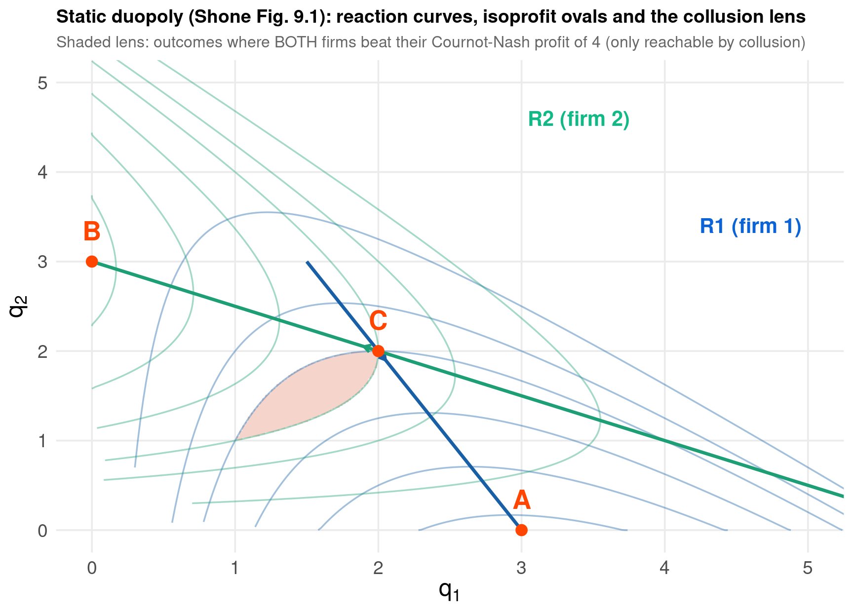
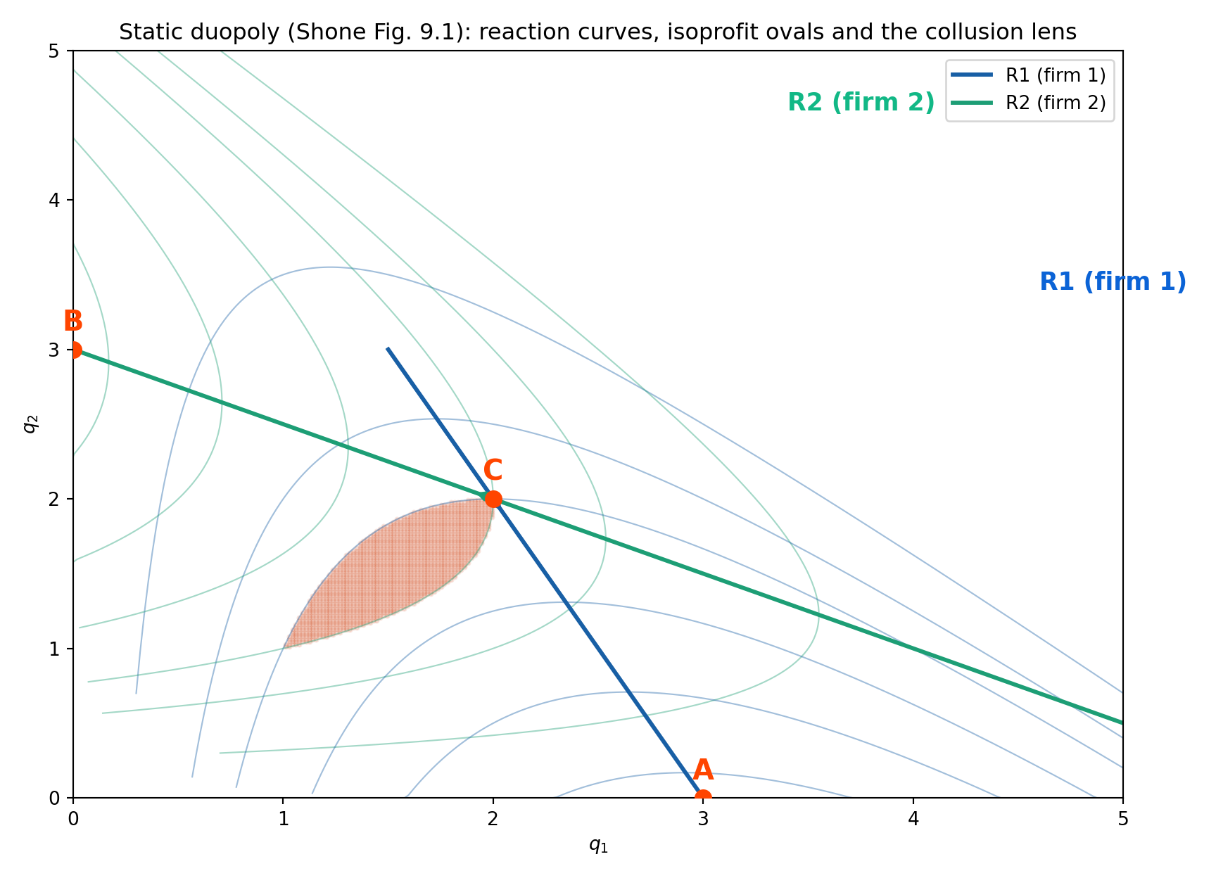
Isoprofit curves. For a fixed profit level \(c\), firm 1’s isoprofit curve in \((q_1,q_2)\) space is found by solving \(\pi_1 = (6-q_1-q_2)q_1 = c\) for \(q_2\):
\[q_2 = 6 - q_1 - \frac{c}{q_1}\]
a family of ovals opening downward. Substituting \(q_1 = 3-\tfrac12 q_2\) (i.e. moving along \(R_1\)) gives \(c = q_1^2\): \(R_1\) is exactly the locus of the tops of firm 1’s isoprofit ovals — the point on each oval where, for that fixed \(q_2\), firm 1’s output \(q_1\) is profit-maximising. The arrow on \(R_1\) points in the direction of rising profit, i.e. toward smaller \(q_2\): firm 1’s most preferred oval collapses to a single point at
By the symmetric argument, \(R_2\) traces the tops of firm 2’s isoprofit ovals, with the arrow pointing toward smaller \(q_1\), collapsing at firm 2’s monopoly point
\[B = (0, 3), \qquad \pi_2(B) = 9\]
Why Cournot–Nash is not Pareto optimal. At \(C=(2,2)\), \(\pi_1(C)=\pi_2(C)=4\). The isoprofit ovals through \(C\) — \(\pi_1 = 4\) and \(\pi_2 = 4\) — cross twice, carving out a lens-shaped region in which both firms earn more than at \(C\) (e.g. at \((1.5,1.5)\), \(\pi_1=\pi_2=4.5>4\)). Every point in this shaded lens Pareto-dominates the Cournot–Nash outcome, but reaching it requires the two firms to jointly restrict output — i.e. collusion — since neither firm’s individually optimal response (its reaction function) leads there. This is Shone’s Figure 9.1.
Code
# Solve the two FOCs as a linear system A q = b directly, rather than by hand:# 6 - 2q1 - q2 = 0 | 2 1 | |q1| |6|# -q1 - 2q2 + 6 = 0 -> | 1 2 | |q2| = |6|A <-matrix(c(2, 1, 1, 2), nrow =2, byrow =TRUE)b <-c(6, 6)q_star <-solve(A, b) # (2, 2)# Reaction curves R1: q1 = 3 - 0.5 q2 , R2: q2 = 3 - 0.5 q1q2_grid <-seq(0, 3, by =0.02)df_react <-tibble(q2 = q2_grid,q1_on_R1 =3-0.5* q2_grid,q1_on_R2 =2* (3- q2_grid))# Firm 1's isoprofit ovals pi1 = (6-q1-q2)q1 = c -> q2 = 6 - q1 - c/q1# Firm 2's isoprofit ovals pi2 = (6-q1-q2)q2 = c -> q1 = 6 - q2 - c/q2iso_levels <-c(1.5, 3, 4, 5.5, 7, 8.5)iso1_list <-list()iso2_list <-list()for (c_lvl in iso_levels) { q1_seq <-seq(0.3, 6, by =0.02) q2_of_q1 <-6- q1_seq - c_lvl / q1_seq keep <- q2_of_q1 >=-0.02 iso1_list[[length(iso1_list) +1]] <-tibble(q1 = q1_seq[keep], q2 =pmax(q2_of_q1[keep], 0), level =factor(c_lvl)) q2_seq <-seq(0.3, 6, by =0.02) q1_of_q2 <-6- q2_seq - c_lvl / q2_seq keep2 <- q1_of_q2 >=-0.02 iso2_list[[length(iso2_list) +1]] <-tibble(q1 =pmax(q1_of_q2[keep2], 0), q2 = q2_seq[keep2], level =factor(c_lvl))}df_iso1 <-bind_rows(iso1_list)df_iso2 <-bind_rows(iso2_list)# Shaded lens: grid points where BOTH firms beat their Cournot-Nash profit (c = 4)grid <-expand.grid(q1 =seq(0, 4, by =0.02), q2 =seq(0, 4, by =0.02))grid$pi1 <- (6- grid$q1 - grid$q2) * grid$q1grid$pi2 <- (6- grid$q1 - grid$q2) * grid$q2lens <- grid[grid$pi1 >4& grid$pi2 >4, ]pts <-tibble(q1 =c(3, 0, 2), q2 =c(0, 3, 2), label =c("A", "B", "C"))ggplot() +geom_tile(data = lens, aes(x = q1, y = q2), fill ="#D85A30", alpha =0.25) +geom_path(data = df_iso1, aes(x = q1, y = q2, group = level), color ="#185FA5", alpha =0.4, linewidth =0.6) +geom_path(data = df_iso2, aes(x = q1, y = q2, group = level), color ="#1D9E75", alpha =0.4, linewidth =0.6) +geom_line(data = df_react, aes(x = q1_on_R1, y = q2), color ="#185FA5", linewidth =1.2) +geom_line(data = df_react, aes(x = q1_on_R2, y = q2), color ="#1D9E75", linewidth =1.2) +geom_segment(aes(x =3-0.5*2.3, y =2.3, xend =3-0.5*1.9, yend =1.9),color ="#185FA5", linewidth =1, arrow =arrow(length =unit(0.2, "cm"))) +geom_segment(aes(x =2.3, y =3-0.5*2.3, xend =1.9, yend =3-0.5*1.9),color ="#1D9E75", linewidth =1, arrow =arrow(length =unit(0.2, "cm"))) +geom_point(data = pts, aes(x = q1, y = q2), size =3.5, color ="#FF4500") +geom_text(data = pts, aes(x = q1, y = q2, label = label), color ="#FF4500", vjust =-1.1, size =7, fontface ="bold") +annotate("text", x =4.6, y =3.4, label ="R1 (firm 1)", color ="#0B63D6", size =5.5, fontface ="bold") +annotate("text", x =3.4, y =4.6, label ="R2 (firm 2)", color ="#12B886", size =5.5, fontface ="bold") +coord_cartesian(xlim =c(0, 5), ylim =c(0, 5)) +labs(x =expression(q[1]), y =expression(q[2]),title ="Static duopoly (Shone Fig. 9.1): reaction curves, isoprofit ovals and the collusion lens",subtitle ="Shaded lens: outcomes where BOTH firms beat their Cournot-Nash profit of 4 (only reachable by collusion)") + theme_lecture
Code
import numpy as npimport sympy as spimport matplotlib.pyplot as plt# Solve the FOCs two ways: (1) linear algebra, (2) symbolically from the profit functionsA = np.array([[2, 1], [1, 2]])b = np.array([6, 6])q_star = np.linalg.solve(A, b)q1, q2 = sp.symbols("q1 q2")pi1 = (9- q1 - q2) * q1 -3* q1pi2 = (9- q1 - q2) * q2 -3* q2foc = [sp.diff(pi1, q1), sp.diff(pi2, q2)]sym_solution = sp.solve(foc, [q1, q2])print("Linear-algebra solution:", q_star)
Cournot’s dynamic assumption: at time \(t\) each firm believes its rival will repeat last period’s output, and chooses its own output to maximise profit now:
“Complete and instantaneous adjustment” means each firm jumps straight to its optimum given last period’s rival output — it is a naive (Cournot) expectation about the rival, not full information about what the rival will do this period. Section 9.3 relaxes the “jump straight to optimum” part via partial adjustment.
Eigenvalues of \(B\) are \(\pm\tfrac12\) — both inside the unit circle, so \(\mathbf{q}_t \to (2,2)\) from any initial output pair, regardless of \(q_{1,0}, q_{2,0}\).
The closed-form solution (matches the static fixed point plus two decaying modes):
Since both roots decay geometrically at rate \(\tfrac12\) per period, convergence is monotone — there is no overshoot, unlike the \(n\ge3\) case on the next slide.
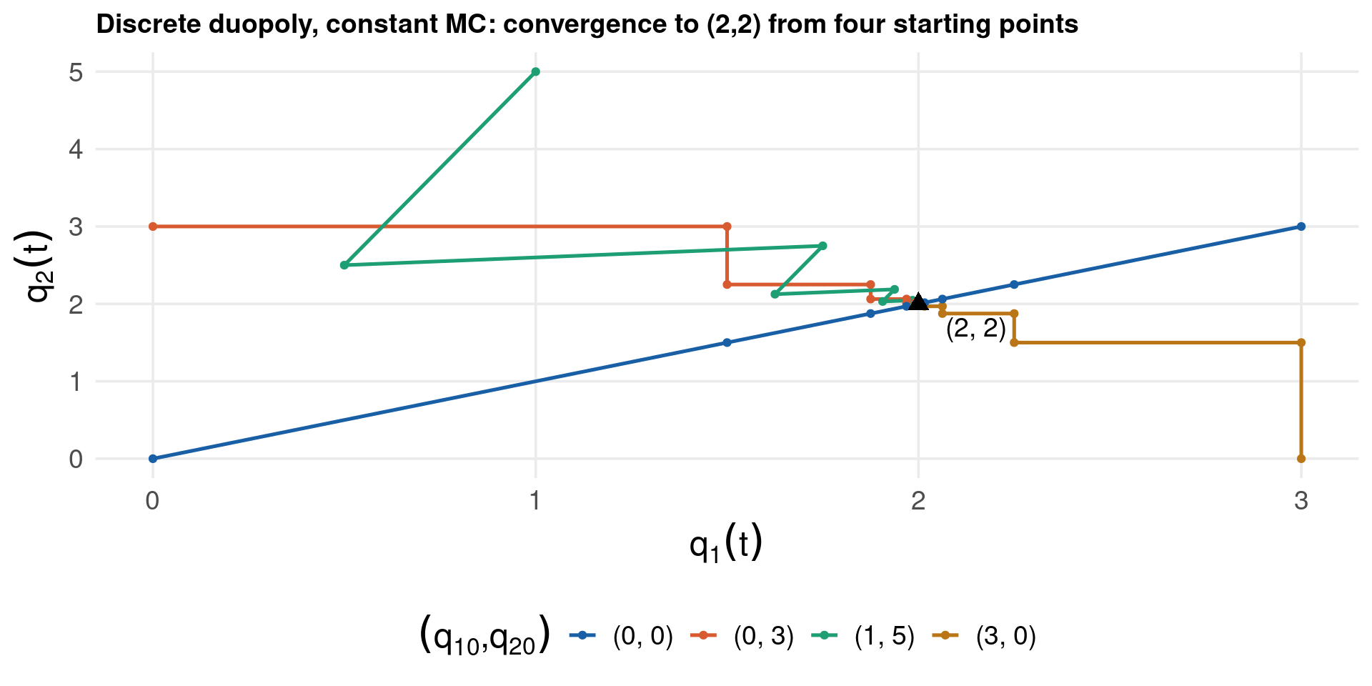
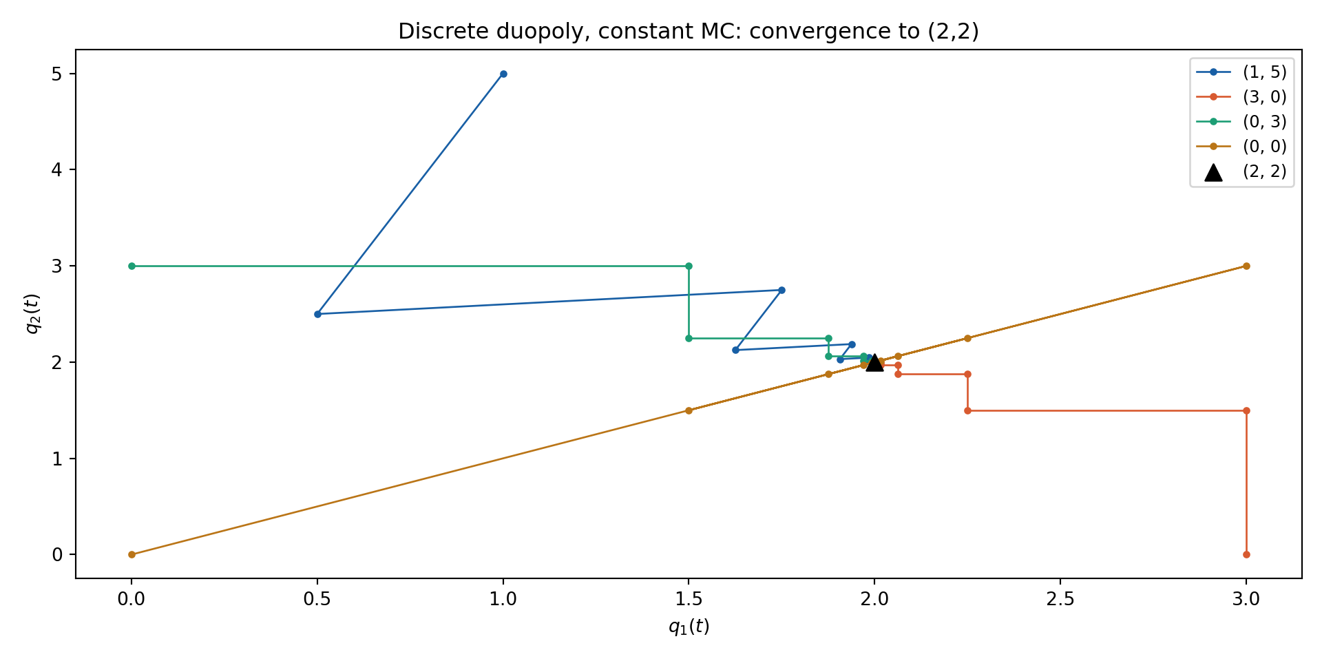
Simulating the discrete tâtonnement — the logic behind simulate_discrete():
Fix the number of firms \(n\), horizon \(T\), and initial outputs \(\mathbf{q}_0 = (q_{1,0}, \dots, q_{n,0})\)
For each period \(t = 1, \dots, T\):
Read last period’s outputs \(\mathbf{q}_{t-1}\)
For each firm \(i\), sum the rivals’ lagged outputs: \(\text{rival\_sum} = \sum_{j\neq i} q_{j,t-1}\)
Compute firm \(i\)’s desired output from its reaction function: \(x_{i,t} = 3 - \tfrac12\,\text{rival\_sum}\)
Set \(q_{i,t} = x_{i,t}\) (complete adjustment — the firm jumps straight to its optimum)
Store \(\mathbf{q}_t\) and repeat until \(t=T\)
Repeat steps 1–3 for each of the four starting points \((q_{1,0},q_{2,0}) \in \{(1,5),(3,0),(0,3),(0,0)\}\)
Plot the trajectories in \((q_1,q_2)\) space — every path should spiral or step onto \((2,2)\)
Code
simulate_discrete <-function(n, T, q0, k =1, cost =c("constant", "increasing")) { cost <-match.arg(cost) q <-matrix(0, T +1, n); q[1, ] <- q0for (t inseq_len(T)) { prev <- q[t, ]for (i inseq_len(n)) { rival_sum <-sum(prev[-i]) x <-if (cost =="constant") 3-0.5* rival_sum else9/8- (1/8) * rival_sum q[t +1, i] <- prev[i] + k * (x - prev[i]) # k = 1: complete adjustment } } q}ics <-list(c(1, 5), c(3, 0), c(0, 3), c(0, 0)) # Shone's four starting pointsdf_phase <-tibble()for (ic in ics) { res <-simulate_discrete(2, 15, ic) df_ic <-tibble(t =0:15, q1 = res[, 1], q2 = res[, 2],ic =glue("({ic[1]}, {ic[2]})")) df_phase <-bind_rows(df_phase, df_ic)}ggplot(df_phase) +aes(x = q1, y = q2, color = ic) +geom_path(linewidth =0.9) +geom_point(size =1.3) +annotate("point", x =2, y =2, size =3.5, shape =17, color ="black") +annotate("text", x =2.15, y =1.7, label ="(2, 2)", color ="black") +scale_color_manual(values =c("#185FA5", "#D85A30", "#1D9E75", "#BA7517"), name =expression((q[10]*","*q[20]))) +labs(x =expression(q[1](t)), y =expression(q[2](t)),title ="Discrete duopoly, constant MC: convergence to (2,2) from four starting points") + theme_lecture
In matrix form, \(\mathbf{q}_t = 3\mathbf{1} - \tfrac12(J - I)\,\mathbf{q}_{t-1}\), where \(J\) is the \(n\times n\) all-ones matrix.
Since \(J\) has eigenvalues \(n\) (once, eigenvector \(\mathbf{1}\)) and \(0\) (\(n-1\) times, any vector orthogonal to \(\mathbf{1}\)), the coefficient matrix \(-\tfrac12(J-I)\) has eigenvalues
\[\boxed{n = 2 \Rightarrow \text{stable} \;(\lambda_1=-\tfrac12), \quad n = 3 \Rightarrow \text{borderline}\;(\lambda_1=-1,\text{ constant oscillation}), \quad n \geq 4 \Rightarrow \text{unstable}\;(|\lambda_1|>1)}\]
This is the Theocharis (1960) instability theorem: under linear demand and constant marginal costs, Cournot tâtonnement is dynamically stable only for duopoly. The symmetric Cournot-Nash equilibrium is \(q_i^* = 6/(n+1)\) for every firm (from \(q^*(1+\tfrac{n-1}{2}) = 3\)).
Step 0 — compute the equilibrium for any \(n\) before simulating anything: the fixed point solves the \(n\times n\) linear system \(\big(I + \tfrac12(J-I)\big)\mathbf{q}^* = 3\mathbf{1}\), so it can be obtained directly with a linear solver (solve() / np.linalg.solve()) for any\(n\) — no need to guess or re-derive \(6/(n+1)\) by hand each time. We verify the closed form this way for \(n=2,\dots,6\) below before moving to the dynamics.
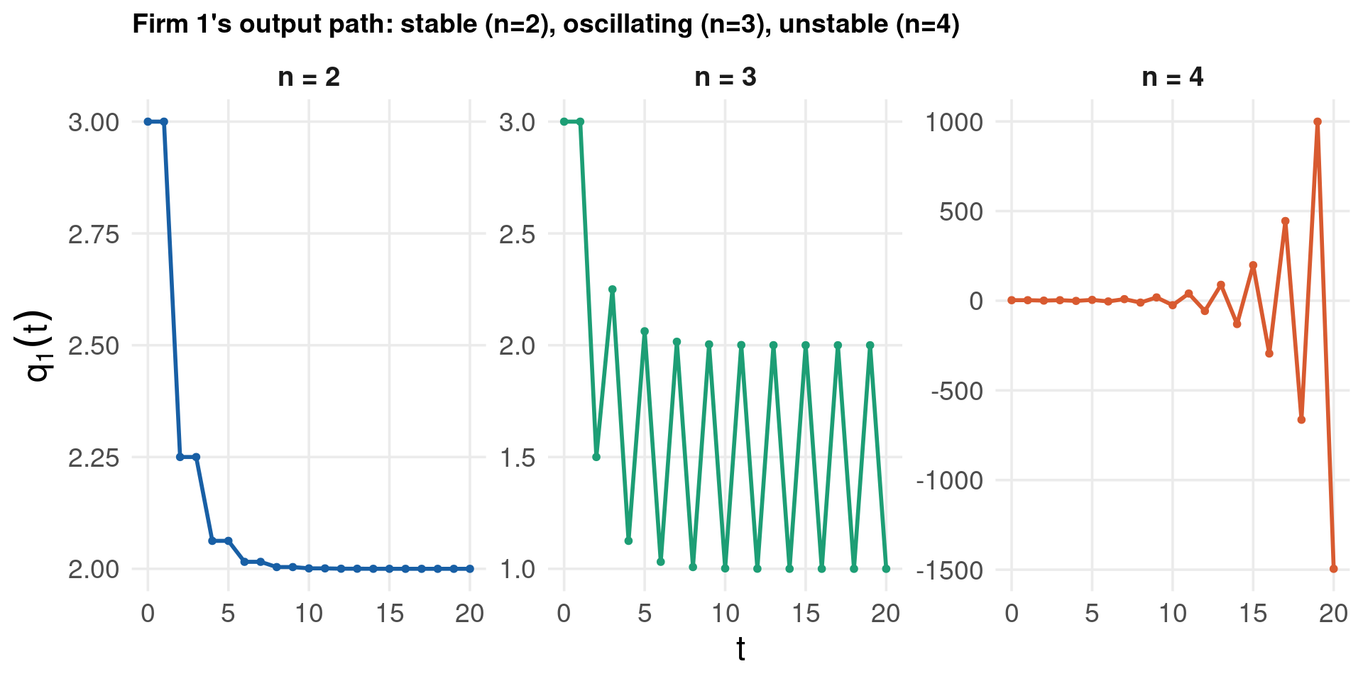
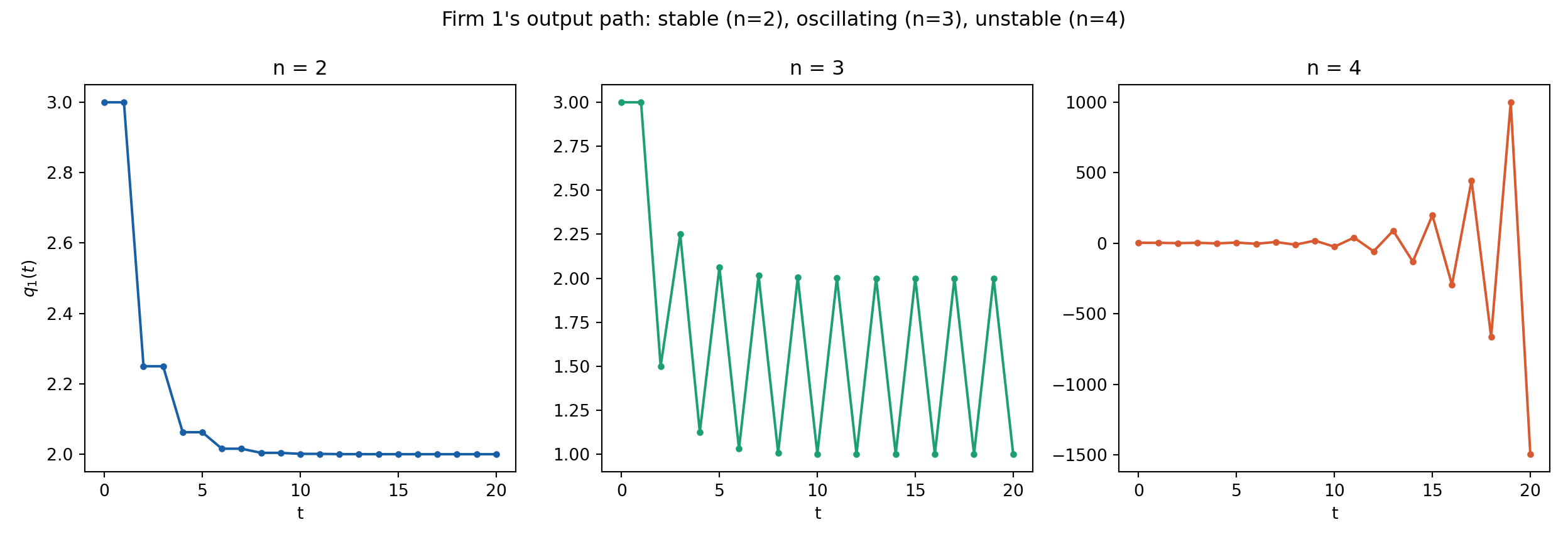
Comparing \(n=2,3,4\) — reusing simulate_discrete() at complete adjustment (\(k=1\)):
For each \(n \in \{2, 3, 4\}\), set the initial condition to a monopoly start: firm 1 at \(q_{1,0}=3\), every other firm at \(0\)
Run the \(n\)-firm recursion \(q_{i,t} = 3 - \tfrac12\sum_{j\neq i}q_{j,t-1}\) for \(T=20\) periods (same inner loop as the duopoly case, generalised to \(n\) firms)
Extract firm 1’s time path \(q_{1,t}\) for each \(n\)
Plot the three paths on separate y-axes (facets) since the \(n=4\) path grows by orders of magnitude relative to \(n=2,3\) — a shared axis would hide the stable and oscillating cases entirely
Read off the qualitative regime directly from the shape: monotone convergence (\(n=2\)), a clean two-period cycle (\(n=3\)), explosive growth (\(n=4\)) — exactly as the eigenvalue \(\lambda_1=-(n-1)/2\) predicts
Code
# Step 0: solve for the equilibrium directly (any n), then check against 6/(n+1)cournot_equilibrium <-function(n, cost =c("constant", "increasing")) { cost <-match.arg(cost) J <-matrix(1, n, n); I <-diag(n)if (cost =="constant") {solve(I +0.5* (J - I), rep(3, n)) } else {solve(I + (1/8) * (J - I), rep(9/8, n)) }}for (n in2:6) {cat("n =", n, " solved q* =", round(cournot_equilibrium(n)[1], 4)," | formula 6/(n+1) =", round(6/ (n +1), 4), "\n")}df_n <-tibble()for (n in2:4) { res <-simulate_discrete(n, 20, q0 =c(3, rep(0, n -1))) # firm 1 starts as monopolist df_this_n <-tibble(t =0:20, q1 = res[, 1], n =glue("n = {n}")) df_n <-bind_rows(df_n, df_this_n)}ggplot(df_n) +aes(x = t, y = q1, color = n) +geom_line(linewidth =1) +geom_point(size =1.2) +facet_wrap(~n, scales ="free_y", nrow =1) +# n=4 explodes: needs its own y-axisscale_color_manual(values =c("#185FA5", "#1D9E75", "#D85A30"), name =NULL, guide ="none") +labs(x ="t", y =expression(q[1](t)),title ="Firm 1's output path: stable (n=2), oscillating (n=3), unstable (n=4)") + theme_lecture
import numpy as npimport matplotlib.pyplot as plt# Step 0: solve for the equilibrium directly (any n), then check against 6/(n+1)def cournot_equilibrium(n, cost="constant"): J = np.ones((n, n)); I = np.eye(n)if cost =="constant":return np.linalg.solve(I +0.5* (J - I), np.full(n, 3.0))return np.linalg.solve(I + (1/8) * (J - I), np.full(n, 9/8))for n inrange(2, 7): solved = cournot_equilibrium(n)[0]print(f"n={n} solved q*={solved:.4f} formula 6/(n+1)={6/(n+1):.4f}")
n=2  solved q*=2.0000  formula 6/(n+1)=2.0000
n=3  solved q*=1.5000  formula 6/(n+1)=1.5000
n=4  solved q*=1.2000  formula 6/(n+1)=1.2000
n=5  solved q*=1.0000  formula 6/(n+1)=1.0000
n=6  solved q*=0.8571  formula 6/(n+1)=0.8571
Same \(J\)-matrix structure as the constant-MC case, but the self-effect is now \(8\) instead of \(2\), shrinking the off-diagonal coefficient from \(\tfrac12\) to \(\tfrac18\).
Eigenvalues of the coefficient matrix \(-\tfrac18(J-I)\):
Stability requires \(\dfrac{n-1}{8}<1 \iff n<9\) — a much wider stable range than \(n<3\) under constant MC. Equilibrium output per firm is \(q_i^* = 9/(n+7)\).
Rising marginal cost dampens each firm’s response to a rival’s output change, so the system settles faster and stays stable for more firms.
Step 0 — solve for both equilibria directly: exactly as on the previous slide, but now with self-coefficient \(\tfrac18\) instead of \(\tfrac12\): \(\big(I+\tfrac18(J-I)\big)\mathbf{q}^*=\tfrac98\mathbf{1}\), verified against \(9/(n+7)\) for \(n=2,\dots,6\) below.
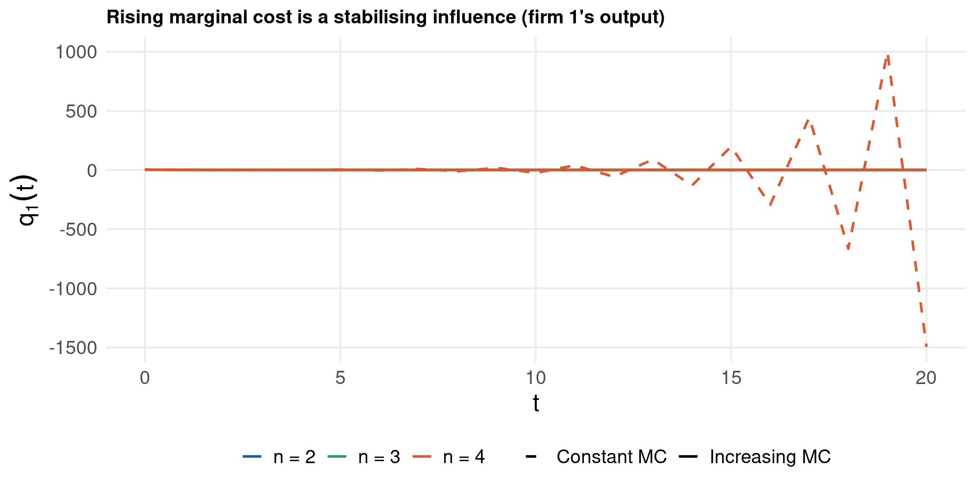
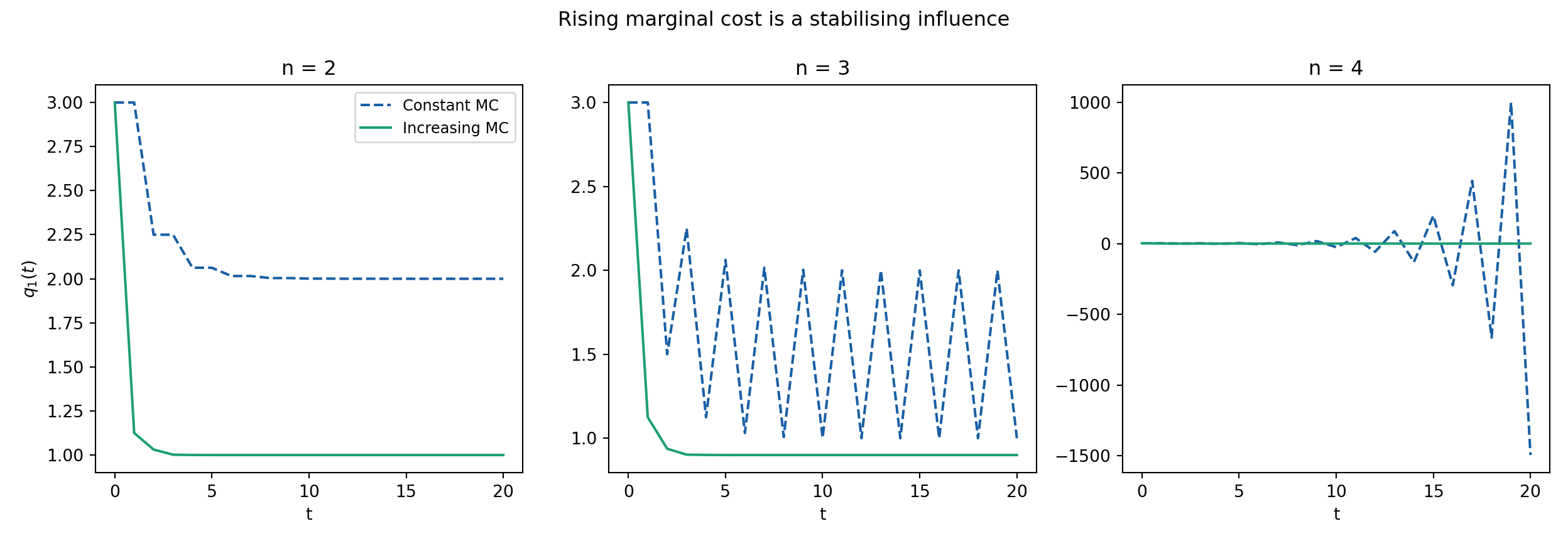
Side-by-side cost regimes — extending simulate_discrete() with a cost switch:
For each \(n \in \{2,3,4\}\), run the recursion twice from the same monopoly start \((3,0,\dots,0)\): once with cost = "constant" (reaction coefficient \(\tfrac12\)) and once with cost = "increasing" (reaction coefficient \(\tfrac18\))
The only change inside the period loop is which reaction function computes \(x_{i,t}\) — everything else (looping over firms, storing the trajectory) is identical to the constant-MC case
Collect both trajectories into one data frame, tagged by cost
Plot firm 1’s path for both regimes on the same panel per \(n\) (dashed = constant MC, solid = increasing MC)
Confirm visually: the solid line always settles faster and lower in amplitude than the dashed line, and remains bounded even at \(n=4\) where the constant-MC path has already exploded
Code
# Step 0: solve both equilibria directly and check against the closed formscournot_equilibrium <-function(n, cost =c("constant", "increasing")) { cost <-match.arg(cost) J <-matrix(1, n, n); I <-diag(n)if (cost =="constant") solve(I +0.5* (J - I), rep(3, n))elsesolve(I + (1/8) * (J - I), rep(9/8, n))}for (n in2:6) {cat("n =", n, " solved q* (incMC) =", round(cournot_equilibrium(n, "increasing")[1], 4)," | formula 9/(n+7) =", round(9/ (n +7), 4), "\n")}df_mc <-tibble()for (n in2:4) { df_const <-tibble(t =0:20, q1 =simulate_discrete(n, 20, c(3, rep(0, n -1)), cost ="constant")[, 1],n =glue("n = {n}"), cost ="Constant MC") df_incr <-tibble(t =0:20, q1 =simulate_discrete(n, 20, c(3, rep(0, n -1)), cost ="increasing")[, 1],n =glue("n = {n}"), cost ="Increasing MC") df_mc <-bind_rows(df_mc, df_const, df_incr)}ggplot(df_mc) +aes(x = t, y = q1, color = n, linetype = cost) +geom_line(linewidth =0.9) +scale_color_manual(values =c("#185FA5", "#1D9E75", "#D85A30"), name =NULL) +scale_linetype_manual(values =c("Constant MC"="dashed", "Increasing MC"="solid"), name =NULL) +labs(x ="t", y =expression(q[1](t)),title ="Rising marginal cost is a stabilising influence (firm 1's output)") + theme_lecture
import numpy as npimport matplotlib.pyplot as plt# Step 0: solve both equilibria directly and check against the closed formsdef cournot_equilibrium(n, cost="constant"): J = np.ones((n, n)); I = np.eye(n)if cost =="constant":return np.linalg.solve(I +0.5* (J - I), np.full(n, 3.0))return np.linalg.solve(I + (1/8) * (J - I), np.full(n, 9/8))for n inrange(2, 7): solved = cournot_equilibrium(n, "increasing")[0]print(f"n={n} solved q*(incMC)={solved:.4f} formula 9/(n+7)={9/(n+7):.4f}")
n=2  solved q*(incMC)=1.0000  formula 9/(n+7)=1.0000
n=3  solved q*(incMC)=0.9000  formula 9/(n+7)=0.9000
n=4  solved q*(incMC)=0.8182  formula 9/(n+7)=0.8182
n=5  solved q*(incMC)=0.7500  formula 9/(n+7)=0.7500
n=6  solved q*(incMC)=0.6923  formula 9/(n+7)=0.6923
So far each firm jumped straight to its optimum every period. We now relax this: each firm closes only a fraction\(k_i\in(0,2)\) of the gap between its desired output and last period’s output:
The desired outputs \(x_{1,t}, x_{2,t}\) are still read off the static reaction functions, evaluated at last period’s rival output — exactly as before:
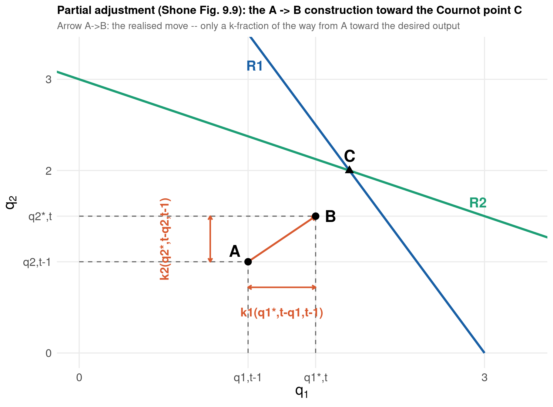
The key distinction:\(x_{1,t}\) is a point on the reaction curve \(R_1\) — it is what firm 1 would choose under complete adjustment. But the firm only moves a fraction \(k_1\) of the way there. So the realised point \((q_{1,t}, q_{2,t})\) generally lies off both reaction curves — this is what makes the phase-plane picture below non-trivial.
For \(k_1=k_2=k\) and initial condition \((q_{1,0},q_{2,0})\), the closed-form solution is:
with the dominant root \(\mu_1(k) = 1-\tfrac32k\). Since \(k>0\), both roots are below \(+1\): stability instead hinges on \(\mu_1(k) > -1\), i.e. \(\boxed{k < 4/3}\) — exactly the \(n=2\) entry of the threshold table on the next slide.
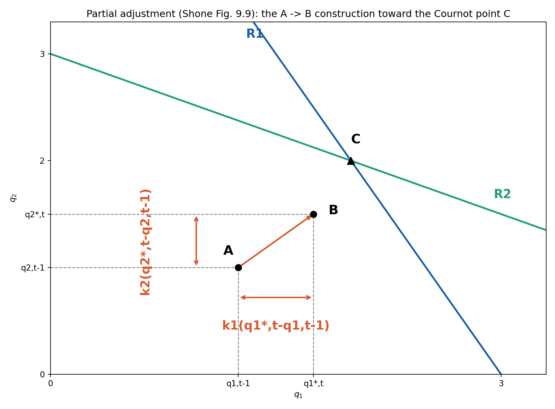
Constructing the single A→B step of Shone’s Figure 9.9:
Pick a starting point below both reaction curves, \(A=(q_{1,t-1},q_{2,t-1})=(1.25, 1)\), and a realised next-period point \(B=(q_{1,t},q_{2,t})=(1.75, 1.5)\) — deliberately not on the line through \(A\) and \(C\), so the construction doesn’t look like a straight shot to equilibrium
Compute each firm’s desired output from the reaction functions at \(A\): \(x_{1,t}=3-\tfrac12 q_{2,t-1}\), \(x_{2,t}=3-\tfrac12 q_{1,t-1}\)
Back out the implied adjustment speeds from \(B=A+(k_1(x_{1,t}-q_{1,t-1}),\, k_2(x_{2,t}-q_{2,t-1}))\): here \(k_1\neq k_2\), since (9.16) never required the two firms to adjust at the same speed
Overlay the two static reaction curves \(R_1, R_2\) as a solid backdrop
Draw the horizontal/vertical partial-adjustment brackets between \(A\) and \(B\), connect \(A\) to \(B\) with an arrow, and mark the Cournot point \(C=(2,2)\) — no line is drawn from \(B\) onward, since the next step would need its own fresh application of steps 2–3 starting from \(B\)
Code
A <-c(q1 =1.25, q2 =1) # point A = (q1,t-1, q2,t-1) -- below BOTH reaction curvesB <-c(q1 =1.75, q2 =1.5) # point B = (q1,t, q2,t) -- the realised, partially-adjusted pointx <-c(3-0.5* A["q2"], 3-0.5* A["q1"]) # desired output (Shone's x1,t, x2,t): read off R1, R2 -- used only inside the recursion, never plotted as its own pointk1 <- (B["q1"] - A["q1"]) / (x[1] - A["q1"]) # implied adjustment speeds firm 1 ...k2 <- (B["q2"] - A["q2"]) / (x[2] - A["q2"]) # ... and firm 2 (need not be equal: eq. 9.16 allows k1 != k2)Cn <-c(2, 2) # Cournot-Nash pointq2_grid <-seq(0, 4, by =0.02)df_react <-tibble(q2 = q2_grid, q1_on_R1 =3-0.5* q2_grid, q1_on_R2 =2* (3- q2_grid))ggplot() +geom_line(data = df_react, aes(x = q1_on_R1, y = q2), color ="#185FA5", linewidth =1.3) +geom_line(data = df_react, aes(x = q1_on_R2, y = q2), color ="#1D9E75", linewidth =1.3) +annotate("text", x =1.3, y =3.15, label ="R1", color ="#185FA5", fontface ="bold", size =6) +annotate("text", x =2.95, y =1.65, label ="R2", color ="#1D9E75", fontface ="bold", size =6) +# axis-projection dashed guides for A = (q1,t-1, q2,t-1)geom_segment(aes(x = A["q1"], y =0, xend = A["q1"], yend = A["q2"]), linetype ="dashed", color ="grey40") +geom_segment(aes(x =0, y = A["q2"], xend = A["q1"], yend = A["q2"]), linetype ="dashed", color ="grey40") +# axis-projection dashed guides for B = (q1,t, q2,t) -- the realised point itselfgeom_segment(aes(x = B["q1"], y =0, xend = B["q1"], yend = B["q2"]), linetype ="dashed", color ="grey40") +geom_segment(aes(x =0, y = B["q2"], xend = B["q1"], yend = B["q2"]), linetype ="dashed", color ="grey40") +# the segment q1,t-1 <-> q1,t: the horizontal distance actually travelled, A -> Bgeom_segment(aes(x = A["q1"], y = A["q2"] -0.28, xend = B["q1"], yend = A["q2"] -0.28),arrow =arrow(length =unit(0.18, "cm"), ends ="both"), color ="#D85A30", linewidth =0.9) +annotate("text", x = (A["q1"] + B["q1"]) /2, y = A["q2"] -0.55,label ="k1(q1*,t-q1,t-1)", size =5.2, color ="#D85A30", fontface ="bold") +# the segment q2,t-1 <-> q2,t: the vertical distance actually travelled, A -> Bgeom_segment(aes(x = A["q1"] -0.28, y = A["q2"], xend = A["q1"] -0.28, yend = B["q2"]),arrow =arrow(length =unit(0.18, "cm"), ends ="both"), color ="#D85A30", linewidth =0.9) +annotate("text", x = A["q1"] -0.62, y = (A["q2"] + B["q2"]) /2,label ="k2(q2*,t-q2,t-1)", size =5.2, color ="#D85A30", fontface ="bold", angle =90) +# the realised move A -> B (no line drawn onward from B to C: that next step needs its own diagram)geom_segment(aes(x = A["q1"], y = A["q2"], xend = B["q1"], yend = B["q2"]),color ="#D85A30", linewidth =1.1, arrow =arrow(length =unit(0.18, "cm"), type ="closed")) +geom_point(aes(x = A["q1"], y = A["q2"]), size =3.5, color ="black") +geom_point(aes(x = B["q1"], y = B["q2"]), size =3.5, color ="black") +geom_point(aes(x = Cn[1], y = Cn[2]), size =3.5, shape =17, color ="black") +annotate("text", x = A["q1"] -0.1, y = A["q2"] +0.12, label ="A", fontface ="bold", size =7) +annotate("text", x = B["q1"] +0.11, y = B["q2"], label ="B", fontface ="bold", size =7) +annotate("text", x = Cn[1], y = Cn[2] +0.16, label ="C", fontface ="bold", size =7) +scale_x_continuous(breaks =c(0, round(A["q1"], 2), round(B["q1"], 2), 3),labels =c("0", "q1,t-1", "q1*,t", "3")) +scale_y_continuous(breaks =c(0, round(A["q2"], 2), round(B["q2"], 2), 2, 3),labels =c("0", "q2,t-1", "q2*,t", "2", "3")) +coord_cartesian(xlim =c(0, 3.3), ylim =c(0, 3.3)) +labs(x =expression(q[1]), y =expression(q[2]),title ="Partial adjustment (Shone Fig. 9.9): the A -> B construction toward the Cournot point C",subtitle ="Arrow A->B: the realised move -- only a k-fraction of the way from A toward the desired output") + theme_lecture
Code
import numpy as npimport matplotlib.pyplot as pltA = np.array([1.25, 1.0]) # point A = (q1,t-1, q2,t-1) -- below BOTH reaction curvesB = np.array([1.75, 1.5]) # point B = (q1,t, q2,t) -- the realised, partially-adjusted pointx = np.array([3-0.5* A[1], 3-0.5* A[0]]) # desired output (Shone's x1,t, x2,t): read off R1, R2 -- used only inside the recursion, never plotted as its own pointk1 = (B[0] - A[0]) / (x[0] - A[0]) # implied adjustment speeds firm 1 ...k2 = (B[1] - A[1]) / (x[1] - A[1]) # ... and firm 2 (need not be equal: eq. 9.16 allows k1 != k2)Cn = np.array([2.0, 2.0]) # Cournot-Nash pointq2_grid = np.linspace(0, 4, 200)q1_on_R1 =3-0.5* q2_gridq1_on_R2 =2* (3- q2_grid)fig, ax = plt.subplots(figsize=(9.5, 7))ax.plot(q1_on_R1, q2_grid, color="#185FA5", linewidth=2.2)ax.plot(q1_on_R2, q2_grid, color="#1D9E75", linewidth=2.2)ax.annotate("R1", (1.3, 3.15), color="#185FA5", fontsize=15, fontweight="bold")ax.annotate("R2", (2.95, 1.65), color="#1D9E75", fontsize=15, fontweight="bold")# axis-projection dashed guides for A and for Bfor pt in (A, B): ax.plot([pt[0], pt[0]], [0, pt[1]], "--", color="grey", linewidth=1) ax.plot([0, pt[0]], [pt[1], pt[1]], "--", color="grey", linewidth=1)# the segments q1,t-1 <-> q1,t and q2,t-1 <-> q2,t: the distance actually travelled, A -> Bax.annotate("", xy=(B[0], A[1] -0.28), xytext=(A[0], A[1] -0.28), arrowprops=dict(arrowstyle="<->", color="#D85A30", linewidth=1.8))ax.annotate("k1(q1*,t-q1,t-1)", ((A[0] + B[0]) /2, A[1] -0.58), color="#D85A30", fontsize=15, fontweight="bold", ha="center")ax.annotate("", xy=(A[0] -0.28, B[1]), xytext=(A[0] -0.28, A[1]), arrowprops=dict(arrowstyle="<->", color="#D85A30", linewidth=1.8))ax.annotate("k2(q2*,t-q2,t-1)", (A[0] -0.62, (A[1] + B[1]) /2), color="#D85A30", fontsize=15, fontweight="bold", ha="center", va="center", rotation=90)# the realised move A -> B (no line drawn onward from B to C: that next step needs its own diagram)ax.annotate("", xy=B, xytext=A, arrowprops=dict(arrowstyle="-|>", color="#D85A30", linewidth=2))ax.scatter(*A, color="black", s=60, zorder=5)ax.scatter(*B, color="black", s=60, zorder=5)ax.scatter(*Cn, color="black", marker="^", s=80, zorder=5)ax.annotate("A", (A[0] -0.1, A[1] +0.12), fontsize=16, fontweight="bold")ax.annotate("B", (B[0] +0.1, B[1]), fontsize=16, fontweight="bold")ax.annotate("C", (Cn[0], Cn[1] +0.16), fontsize=16, fontweight="bold")ax.set_xticks([0, A[0], B[0], 3]); ax.set_xticklabels(["0", "q1,t-1", "q1*,t", "3"])ax.set_yticks([0, A[1], B[1], 2, 3]); ax.set_yticklabels(["0", "q2,t-1", "q2*,t", "2", "3"])ax.set_xlim(0, 3.3); ax.set_ylim(0, 3.3)
(0.0, 3.3)
(0.0, 3.3)
Code
ax.set_xlabel(r"$q_1$"); ax.set_ylabel(r"$q_2$")ax.set_title("Partial adjustment (Shone Fig. 9.9): the A -> B construction toward the Cournot point C")plt.tight_layout(); plt.show()
The system starts at time \(t-1\) at point \(A = (q_{1,t-1}, q_{2,t-1})\) — its two dashed guide lines drop straight onto the axis values \(q_{1,t-1}\) and \(q_{2,t-1}\)
Firm 1’s desired output \(x_{1,t}=3-\tfrac12 q_{2,t-1}\) is read off \(R_1\), and firm 2’s desired output \(x_{2,t}=3-\tfrac12 q_{1,t-1}\) is read off \(R_2\) — these desired values are not separately plotted as a point; they only enter the formula for how far the firm actually moves
Under partial adjustment each firm only moves a fraction of the way from \(A\) toward its own desired output: the two double-headed arrows show the realised horizontal step \(k_1(q_{1,t}-q_{1,t-1})\) and vertical step \(k_2(q_{2,t}-q_{2,t-1})\), landing at \(B=(q_{1,t},q_{2,t})\) — its own dashed guide lines drop onto the axis values \(q_{1,t}\) and \(q_{2,t}\), exactly as \(A\)’s did. Note \(B\) lies off both reaction curves — partial adjustment never lands back on \(R_1\) or \(R_2\)
\(A\), \(B\) and \(C\) are not collinear here: \(k_1\neq k_2\) in this example, so the single realised step \(A\to B\) is not simply “part way along the line to \(C\)” — nothing in one step guarantees the direction of travel points at the equilibrium, let alone the distance
What is not obvious just from this one step: whether repeating the same construction, with \(B\) as the new “\(A\)”, eventually converges on the Cournot–Nash solution \(C=(2,2)\), and if so, what shape the resulting sequence of steps takes — a straight line, a curve, a spiral, or something that overshoots and oscillates
Answering this requires solving the linear difference equation explicitly, not just staring at one step of the diagram — which is exactly what the closed-form solution on the Theory tab does
With equal speeds \(k_1=k_2=k\), both eigenvalues of \(M(k)\) are real and positive whenever \(k<2/3\), so repeated steps curve smoothly into \(C\) with no oscillation — a qualitatively different shape from the complete-adjustment (\(k=1\)) cobweb of two slides ago
Substituting the reaction function gives \(\mathbf{q}_t = 3k\mathbf{1} + M(k)\,\mathbf{q}_{t-1}\) with \(M(k) = (1-k)I - \tfrac{k}{2}(J-I)\) for constant MC.
Complete adjustment (\(k=1\)) recovers the Theocharis results of the previous slides as the special case \(k=1\); the eigenvalue algebra below just re-does the same \(J\)-matrix trick with \(M(k)\) instead of \(-\tfrac12(J-I)\).
At \(k=k^*\) the dominant root is exactly \(-1\): the system settles into a permanent two-period oscillation. Above \(k^*\), output paths explode.
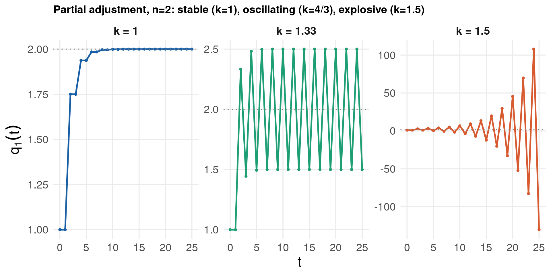
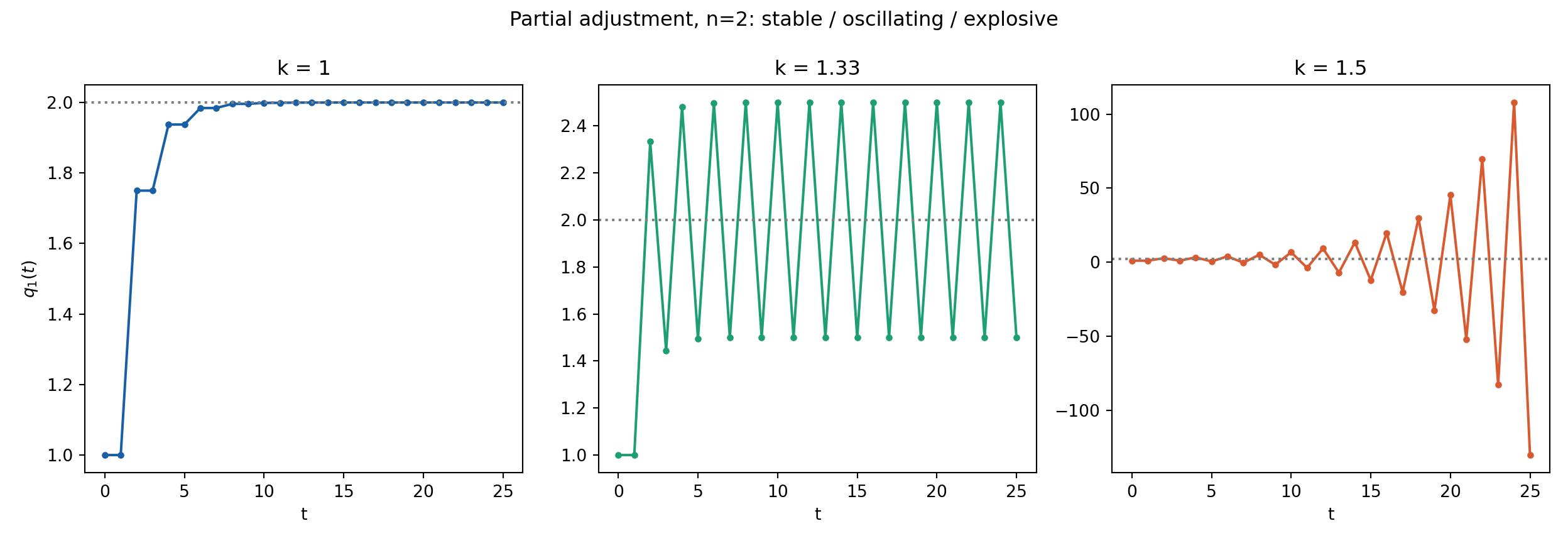
Sweeping the adjustment speed \(k\) — reusing simulate_discrete() with its k argument:
Fix \(n=2\) and pick one initial condition, e.g. \((q_{1,0},q_{2,0})=(1,4)\)
For each candidate speed \(k \in \{1,\; 4/3,\; 1.5\}\) (below, at, and above the threshold \(k^*(2)=4/3\)):
Run the same period loop as before, but replace the complete-adjustment update with the partial-adjustment step \(q_{i,t} = q_{i,t-1} + k\,(x_{i,t} - q_{i,t-1})\)
Everything else — computing rival sums, the reaction function \(x_{i,t}\) — is unchanged
Collect the three trajectories, tag each by its \(k\)
Plot on separate y-axes (facets), since the \(k=1.5\) path grows without bound while \(k=1\) and \(k=4/3\) stay bounded
Confirm: \(k=1\) converges monotonically, \(k=4/3=k^*\) locks into an exact 2-cycle, \(k=1.5>k^*\) diverges — matching \(\mu_1(k)\) crossing \(-1\)
Code
ks <-c(1, 4/3, 1.5)df_k <-tibble()for (k in ks) { res <-simulate_discrete(2, 25, q0 =c(1, 4), k = k) df_this_k <-tibble(t =0:25, q1 = res[, 1], k =glue("k = {round(k, 2)}")) df_k <-bind_rows(df_k, df_this_k)}ggplot(df_k) +aes(x = t, y = q1, color = k) +geom_line(linewidth =1) +geom_point(size =1) +geom_hline(yintercept =2, linetype ="dotted", color ="grey55") +facet_wrap(~k, scales ="free_y", nrow =1) +# k=1.5 explodes: needs its own y-axisscale_color_manual(values =c("#185FA5", "#1D9E75", "#D85A30"), name =NULL, guide ="none") +labs(x ="t", y =expression(q[1](t)),title ="Partial adjustment, n=2: stable (k=1), oscillating (k=4/3), explosive (k=1.5)") + theme_lecture
Code
import numpy as npimport matplotlib.pyplot as pltfig, axes = plt.subplots(1, 3, figsize=(13, 4.5)) # k=1.5 explodes: needs its own y-axisfor ax, (k, c) inzip(axes, zip([1, 4/3, 1.5], ["#185FA5", "#1D9E75", "#D85A30"])): res = simulate_discrete(2, 25, np.array([1.0, 4.0]), k=k) ax.plot(range(26), res[:, 0], color=c, marker="o", markersize=3) ax.axhline(2, linestyle=":", color="grey") ax.set_title(f"k = {round(k, 2)}"); ax.set_xlabel("t")axes[0].set_ylabel(r"$q_1(t)$")fig.suptitle("Partial adjustment, n=2: stable / oscillating / explosive")plt.tight_layout(); plt.show()
For \(n\) symmetric firms with common speed \(k\), in matrix form \(\dot{\mathbf{q}} = 3k\mathbf{1} - A\mathbf{q}\) with
\[A = kI + \frac{k}{2}(J - I)\]
For increasing MC (\(TC_i=3q_i^2\)), the same argument with self-coefficient \(8\) instead of \(2\) gives \(A = kI + \tfrac{k}{8}(J-I)\).
Isoclines: setting \(\dot q_1=0\) and \(\dot q_2=0\) for \(n=2\) recovers exactly the two static reaction functions from the very first duopoly slide, \(q_1=3-\tfrac12q_2\) and \(q_2=3-\tfrac12q_1\) — the reaction curves are not just a static best-response device, they are literally the zero-motion isoclines of the continuous dynamic system, and their intersection is the fixed point \((2,2)\).
Eigenvalues of \(A\): on \(\mathbf{1}\), \(\;k + \tfrac{k}{2}(n-1) = k\dfrac{n+1}{2} > 0\); on any vector orthogonal to \(\mathbf{1}\), \(\;k - \tfrac{k}{2} = \tfrac{k}{2} > 0\). Both eigenvalues of \(A\) are positive for every \(n\) and every \(k>0\), so the Jacobian \(-A\) has both eigenvalues strictly negative — the equilibrium \(q_i^*=6/(n+1)\) is a stable node for any number of firms.
Discrete vs. continuous — the key contrast
This is the central lesson of the chapter: the Theocharis instability (\(n\ge 3\)) is a purely discrete-time phenomenon. It arises because a discrete lag can overshoot the equilibrium once the coefficient magnitude exceeds 1. Continuous adjustment has no “period,” so there is nothing to overshoot — for this linear-demand, linear-cost model the continuous-time equilibrium is unconditionally stable, and \(k\) only sets the speed, never the stability, of convergence. (For \(n=3,5,7,\dots\) the determinant of \(-A\) is negative simply because the product of an odd number of negative eigenvalues is negative — this is not evidence of a saddle point, since a saddle requires eigenvalues of mixed sign, and here every eigenvalue of \(-A\) is negative.) This is not a new result: McManus & Quandt (1961) first proved that replacing Theocharis’s discrete tâtonnement with continuous, imperfect adjustment restores unconditional stability for any \(n\) — our eigenvalue derivation reconstructs their result from first principles.
Since \(k/8 < k/2\), increasing MC also converges faster than constant MC, exactly as in the discrete case.
Simulating the continuous-time system — the logic behind oligopoly_ode():
Define a right-hand-side function rhs(t, q, parms) that, given the current state vector \(\mathbf{q}\), computes \(\dot q_i\) for every firm \(i\): sum the rivals’ current outputs, form the reaction-function target \(x_i\), and return \(k(x_i - q_i)\)
Pass rhs to an ODE solver (deSolve::ode in R, scipy.integrate.solve_ivp in Python) together with the initial condition \(\mathbf{q}(0)\) and a time grid (here \(t \in [0, 8]\))
The solver integrates the system internally — there is no explicit period-by-period loop to write, unlike the discrete case
Repeat step 2 for each of the four starting points \((q_1(0), q_2(0))\)
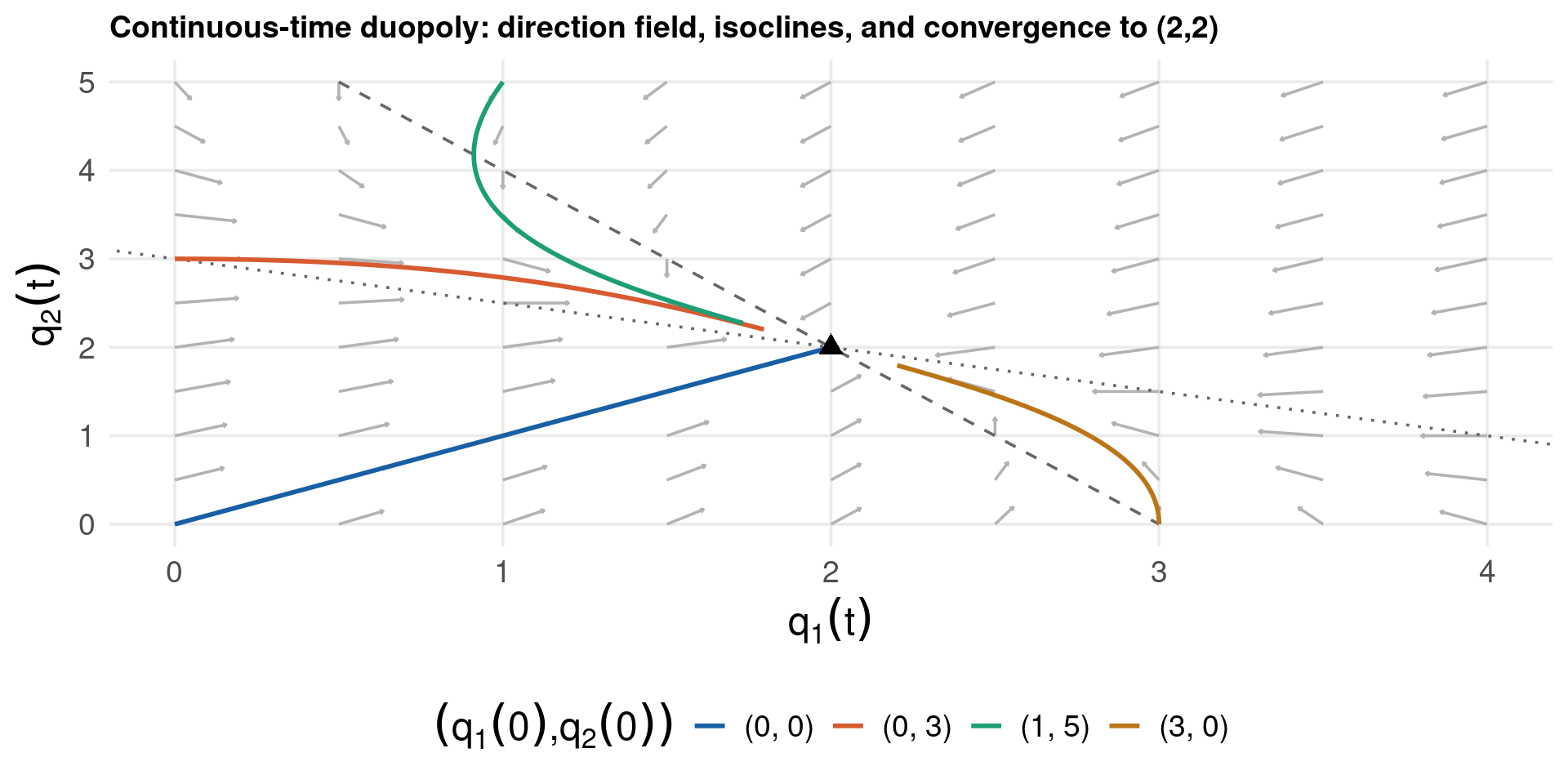
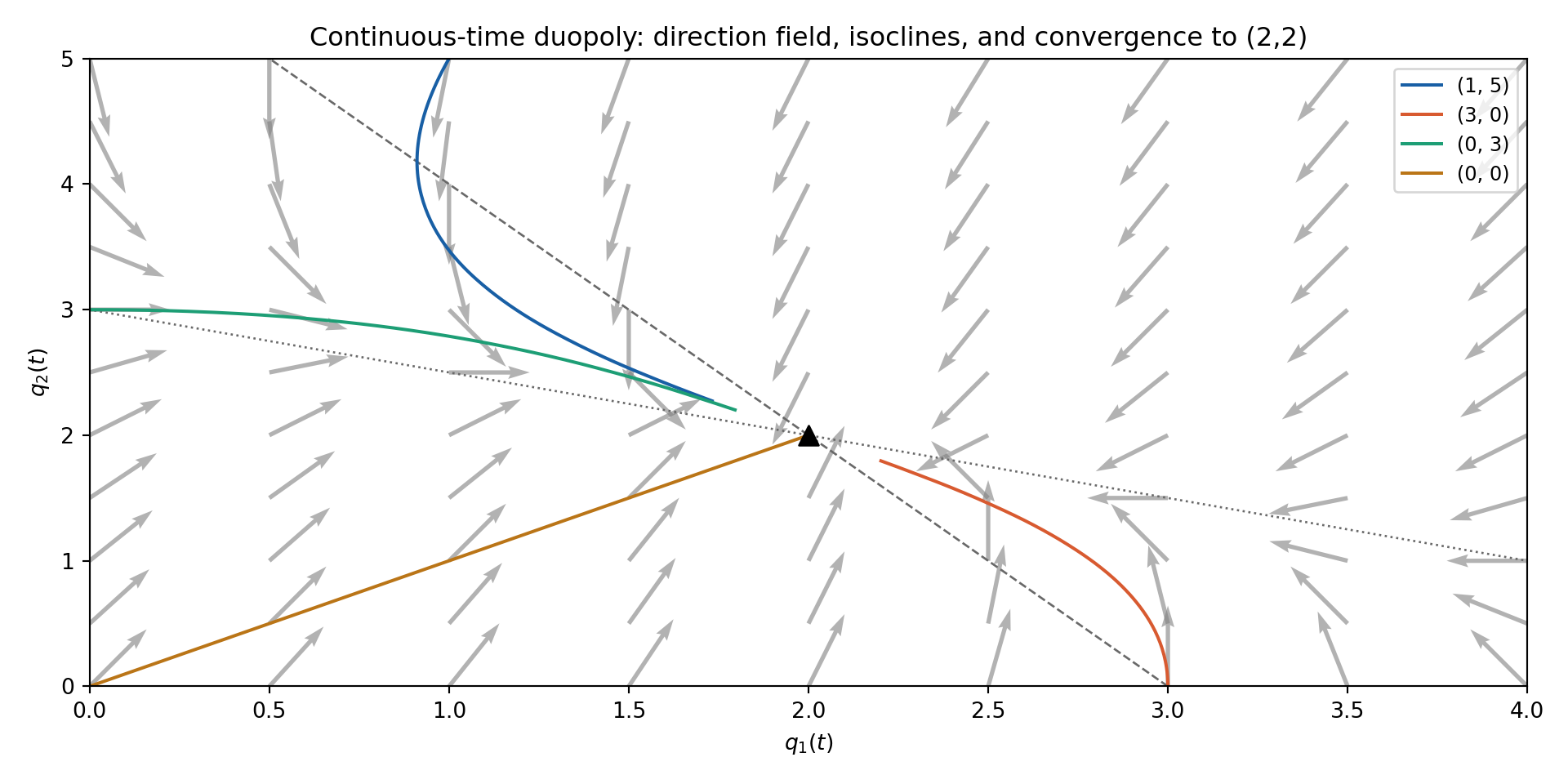
Plot the resulting trajectories in \((q_1, q_2)\) space: unlike the discrete phase diagram, these are smooth curves, not zig-zag step paths, and none of them overshoot \((2,2)\)
Add the direction field: evaluate \((\dot q_1,\dot q_2)\) on a grid of \((q_1,q_2)\) points, normalise each vector’s length for legibility, and draw it as a short arrow (geom_segment/ax.quiver) — every trajectory should follow the local arrow direction at each point it passes through
Overlay the two isoclines\(q_1=3-\tfrac12q_2\) and \(q_2=3-\tfrac12q_1\) (the reaction functions) — every arrow should point purely vertically when crossing the \(\dot q_1=0\) line and purely horizontally when crossing the \(\dot q_2=0\) line
Code
oligopoly_ode <-function(n, k, cost =c("constant", "increasing")) { cost <-match.arg(cost)function(t, q, parms) { dq <-numeric(n)for (i inseq_len(n)) { rival_sum <-sum(q[-i]) x <-if (cost =="constant") 3-0.5* rival_sum else9/8- (1/8) * rival_sum dq[i] <- k * (x - q[i]) }list(dq) }}ics_c <-list(c(1, 5), c(3, 0), c(0, 3), c(0, 0))df_cont <-tibble()for (ic in ics_c) { sol <-ode(y = ic, times =seq(0, 8, by =0.05),func =oligopoly_ode(2, k =0.5), parms =NULL) df_ic <-as_tibble(as.data.frame(sol)) %>%rename(q1 =`1`, q2 =`2`) %>%mutate(ic =glue("({ic[1]}, {ic[2]})")) df_cont <-bind_rows(df_cont, df_ic)}# Direction field: q1-dot = k(3 - 0.5 q2 - q1), q2-dot = k(3 - 0.5 q1 - q2)grid_q <-expand.grid(q1 =seq(0, 4, by =0.5), q2 =seq(0, 5, by =0.5))grid_q$dq1 <-0.5* (3-0.5* grid_q$q2 - grid_q$q1)grid_q$dq2 <-0.5* (3-0.5* grid_q$q1 - grid_q$q2)grid_q$len <-sqrt(grid_q$dq1^2+ grid_q$dq2^2) +1e-6grid_q$dq1 <- grid_q$dq1 / grid_q$len *0.2# normalise arrow length for readabilitygrid_q$dq2 <- grid_q$dq2 / grid_q$len *0.2# Isoclines: q1-dot=0 is q1=3-0.5q2 (the R1 reaction line); q2-dot=0 is q2=3-0.5q1 (R2)q2_grid <-seq(0, 5, by =0.05)df_isoclines <-tibble(q2 = q2_grid, iso1 =3-0.5* q2, iso2 =2* (3- q2))ggplot() +geom_segment(data = grid_q, aes(x = q1, y = q2, xend = q1 + dq1, yend = q2 + dq2),arrow =arrow(length =unit(0.06, "cm")), color ="grey70") +geom_line(data = df_isoclines, aes(x = iso1, y = q2), color ="grey40", linetype ="dashed") +geom_line(data = df_isoclines, aes(x = iso2, y = q2), color ="grey40", linetype ="dotted") +geom_path(data = df_cont, aes(x = q1, y = q2, color = ic), linewidth =1) +annotate("point", x =2, y =2, size =3.5, shape =17, color ="black") +coord_cartesian(xlim =c(0, 4), ylim =c(0, 5)) +scale_color_manual(values =c("#185FA5", "#D85A30", "#1D9E75", "#BA7517"), name =expression((q[1](0)*","*q[2](0)))) +labs(x =expression(q[1](t)), y =expression(q[2](t)),title ="Continuous-time duopoly: direction field, isoclines, and convergence to (2,2)") + theme_lecture
ax.set_xlabel(r"$q_1(t)$"); ax.set_ylabel(r"$q_2(t)$")ax.set_title("Continuous-time duopoly: direction field, isoclines, and convergence to (2,2)")ax.legend(fontsize=9); plt.tight_layout(); plt.show()
Extending oligopoly_ode() across \(n\) and cost regimes:
For each \(n \in \{2,3,4\}\), build the monopoly initial condition \((3,0,\dots,0)\)
Solve the ODE system twice from that initial condition: once with cost = "constant", once with cost = "increasing" — the oligopoly_ode() factory from the previous slide already supports both via its cost argument
Extract firm 1’s continuous path \(q_1(t)\) from each solution object
Stack all six paths (\(3\) values of \(n\)\(\times\)\(2\) cost regimes) into one long data frame / set of arrays
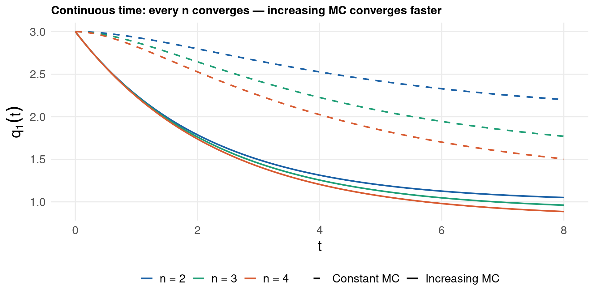
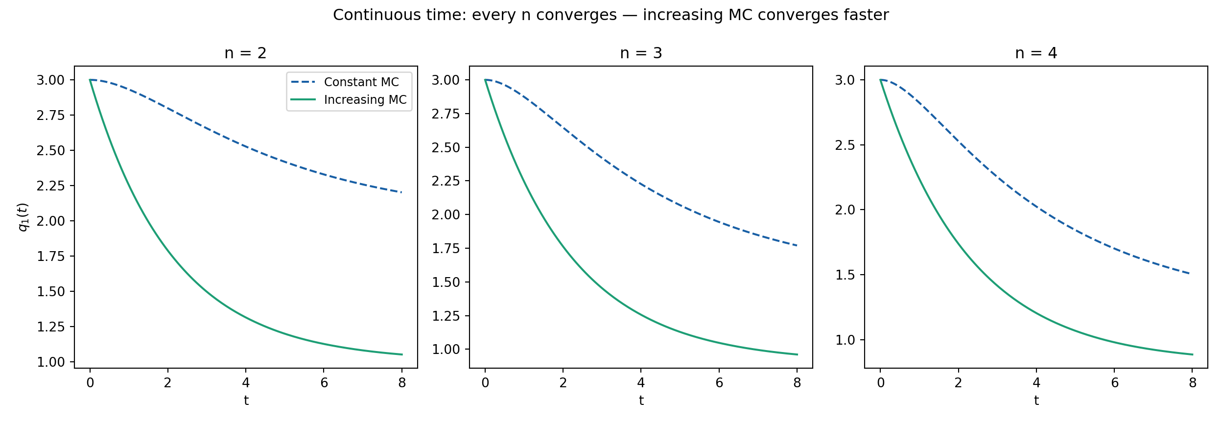
Plot \(q_1(t)\) against \(t\), one panel per \(n\), dashed vs. solid line for the two cost regimes — every curve should settle smoothly with no oscillation or explosion, confirming the “always stable” result for all six cases simultaneously
Code
df_cont_n <-tibble()for (n in2:4) { q0 <-c(3, rep(0, n -1)) df_const <-as_tibble(as.data.frame(ode(y = q0, times =seq(0, 8, 0.05),func =oligopoly_ode(n, k =0.5, cost ="constant"), parms =NULL))) %>%transmute(time, q1 =`1`, n =glue("n = {n}"), cost ="Constant MC") df_incr <-as_tibble(as.data.frame(ode(y = q0, times =seq(0, 8, 0.05),func =oligopoly_ode(n, k =0.5, cost ="increasing"), parms =NULL))) %>%transmute(time, q1 =`1`, n =glue("n = {n}"), cost ="Increasing MC") df_cont_n <-bind_rows(df_cont_n, df_const, df_incr)}ggplot(df_cont_n) +aes(x = time, y = q1, color = n, linetype = cost) +geom_line(linewidth =0.9) +scale_color_manual(values =c("#185FA5", "#1D9E75", "#D85A30"), name =NULL) +scale_linetype_manual(values =c("Constant MC"="dashed", "Increasing MC"="solid"), name =NULL) +labs(x ="t", y =expression(q[1](t)),title ="Continuous time: every n converges — increasing MC converges faster") + theme_lecture
Before leaving linear oligopoly for the nonlinear R&D model, we finish the continuous-time comparison across \(n\) properly: not just simulated trajectories (previous slide) but the actual roots that govern them, exactly as Shone’s Table 9.3 tabulates — and, on the next tab, exactly why those roots take the form they do.
For \(n\) identical firms with partial-adjustment speed \(k\), the continuous-time system is \(\dot{\mathbf q} = c\mathbf 1 + B_n\mathbf q\) with
where \(J\) is the \(n\times n\) matrix of ones (every entry \(=1\)). Both forms are the special structure \(B_n = \alpha I + \beta J\) for scalar constants \(\alpha,\beta\) (functions of \(k\) only, not of \(n\)) — and matrices of this form have eigenvalues that can be read off without ever forming the characteristic polynomial by hand, because \(I\) and \(J\) share the same eigenvectors:
\[B_n\mathbf v = (\alpha I+\beta J)\mathbf v = \alpha\mathbf v + \beta(J\mathbf v) \quad\Longrightarrow\quad \lambda(B_n) = \alpha + \beta\,\lambda(J)\]
So the whole problem reduces to finding the eigenvalues of the plain ones-matrix \(J\), which has an elementary closed form:
\[J\mathbf 1 = n\mathbf 1 \quad(\lambda = n,\text{ eigenvector } \mathbf 1 = (1,\dots,1)^\top), \qquad J\mathbf v = 0 \text{ for any } \mathbf v \perp \mathbf 1 \quad(\lambda = 0,\ \times(n-1))\]
(the second fact holds because every row of \(J\) is \((1,\dots,1)\), so \(J\mathbf v = (\mathbf 1^\top\mathbf v)\mathbf 1 = 0\) whenever \(\mathbf v\)’s entries sum to zero — an \((n-1)\)-dimensional space of such vectors). Substituting \(\lambda(J)\in\{n,0\}\) into \(\lambda(B_n)=\alpha+\beta\lambda(J)\), with \((\alpha,\beta)=(-\tfrac{k}{2},-\tfrac{k}{2})\) for constant MC and \((\alpha,\beta)=(-\tfrac{7k}{8},-\tfrac{k}{8})\) for increasing MC, gives:
This is a genuine derivation, not a lookup: every root in Table 9.3 is \(\alpha + \beta n\) or \(\alpha\) alone, for the \((\alpha,\beta)\) pair appropriate to the cost regime.
\(n\)
Constant MC roots
Increasing MC roots
2
\(-\tfrac{3k}{2},\ -\tfrac{k}{2}\)
\(-\tfrac{9k}{8},\ -\tfrac{7k}{8}\)
3
\(-2k,\ -\tfrac{k}{2}\)
\(-\tfrac{5k}{4},\ -\tfrac{7k}{8}\)
4
\(-\tfrac{5k}{2},\ -\tfrac{k}{2}\)
\(-\tfrac{11k}{8},\ -\tfrac{7k}{8}\)
All roots are negative (stable) for every \(n\) shown — the continuous-time model never loses stability the way the discrete model does. Two patterns matter:
Increasing MC always dominates less negative than it looks — but always beats constant MC: compare each row’s dominant (least negative) root; increasing MC’s is always closer to zero, i.e. still stabilising, but the gap between the two regimes narrows as \(n\) grows
Both dominant roots grow more negative in magnitude as \(n\) rises, meaning convergence actually gets faster, not slower, as more firms are added — the discrete-time instability result (\(n\geq 3\) unstable) has no continuous-time counterpart
Computing Table 9.3 two ways — numerically and symbolically, not just looked up:
Numeric check (R and Python): for each \(n \in \{2,3,4\}\), build \(J\), form \(B_n\) at \(k=1\), and call eigen() / np.linalg.eig() — fast, but only ever gives you a decimal number for one specific \(k\)
Exact rational check (R): compute eigen(J) on the plain ones-matrix — this returns the exact integers \(n\) and \(0\) with no \(k\) involved at all — then apply \(\lambda(B_n)=\alpha+\beta\lambda(J)\) by hand with the exact fractions \((\alpha,\beta)\), displayed via MASS::fractions(), to recover each root as a clean fraction of \(k\)
True symbolic solve (Python, sympy): build \(B_n\) as a sympy.Matrix with \(k\) left as an actual symbol (sympy.Symbol), then call .eigenvals() — this solves the characteristic polynomial \(\det(B_n-\lambda I)=0\)algebraically, returning exact expressions like \(-3k/2\) together with their multiplicities, valid for every\(k\) simultaneously
Confirm all three routes — numeric, exact-fraction, and symbolic — agree with Table 9.3 for every one of the six \((n,\text{cost})\) combinations
Code
# --- Step 1: numeric check at k = 1 ---k <-1build_B <-function(n, cost =c("constant", "increasing")) { cost <-match.arg(cost) J <-matrix(1, n, n) I <-diag(n)if (cost =="constant") -k /2* (J + I) else-(7* k /8) * I - (k /8) * J}roots_tbl <-tibble()for (n in2:4) { ev_const <-sort(round(eigen(build_B(n, "constant"))$values, 3)) ev_incr <-sort(round(eigen(build_B(n, "increasing"))$values, 3)) roots_tbl <-bind_rows(roots_tbl, tibble(n = n,root_constant_dominant = ev_const[1], root_constant_other = ev_const[2],root_increasing_dominant = ev_incr[1], root_increasing_other = ev_incr[length(ev_incr)] ))}cat("Numeric check (k = 1):\n"); print(roots_tbl)# --- Step 2: WHERE the roots come from -- exact fractions via eigen(J) + the affine rule lambda(B) = alpha + beta*lambda(J) ---# alpha, beta are the two EXACT rational coefficients read straight off B_n = alpha*I + beta*Jcoef_const <-c(alpha =-1/2, beta =-1/2) # constant MC: B = -k/2 I - k/2 Jcoef_incr <-c(alpha =-7/8, beta =-1/8) # increasing MC: B = -7k/8 I - k/8 Jfrac_str <-function(x) unique(attr(MASS::fractions(x), "fracs")) # pull the "-3/2"-style stringscat("\nExact fractions of k, derived from eigen(J) (not from eigen(B) at k=1):\n")for (n in2:4) { lambda_J <-round(eigen(matrix(1, n, n))$values) # exact: n once, 0 (n-1) times -- no k involved root_const <-frac_str(coef_const["alpha"] + coef_const["beta"] * lambda_J) root_incr <-frac_str(coef_incr["alpha"] + coef_incr["beta"] * lambda_J)cat("n =", n, " constant MC roots (x k):", root_const," | increasing MC roots (x k):", root_incr, "\n")}
Parker, Whitby & Tobias (2000) replace price/quantity competition with competition through product quality, built up by investment in R&D. Two firms, \(A\) and \(B\), choose how many resources to devote to research:
\(\bar S_t = k^A_t S^A_t + k^B_t S^B_t\) is the market-share-weighted industry-average quality standard. The market-share rows are Shone’s own extension — Parker et al.’s original model stops at resources and quality.
Figure 9.15’s structure is genuinely a time \(t\) vs. time \(t+1\) comparison, not a single-period flow: resources devoted to R&D in period \(t\) determine that same period’s quality standard; the competitive advantage this reveals in period \(t\) is what then alters the market share for period \(t+1\) — and, via Table 9.4’s resource equation, also feeds directly into next period’s R&D resources \(R^i_{t+1}\).
Time t
R&D resources \(R^i_t\)
↓
Quality standard \(S^i_t=\frac{2m^i}{\pi}\arctan(R^i_t)-n^i\)
↓
Competitive advantage in period t: \(S^i_t \gt S^{-i}_t\)?
↳ next period, \(R^i_{t+1}\) becomes the new “time \(t\)” box, and the whole comparison repeats
Notice the asymmetry in timing: \(R^i_t \to S^i_t\) and the advantage check all happen within period \(t\); only the consequences of that period-\(t\) advantage — the new market share and the new resource budget — are dated \(t+1\)
\(\bar S_t = k^A_tS^A_t+k^B_tS^B_t\), the industry-average quality standard, is itself computed from period-\(t\) quantities, then used to update period-\((t+1)\) market shares
The S-shaped\(\arctan\) curve captures diminishing returns: low R&D buys little quality, mid-range R&D buys a lot, high R&D runs into diminishing returns
\(m\) controls the steepness of the S-curve; \(n\) shifts its inflexion point
Because the quality function is bounded and \(\max[0,\cdot]\) clips resources at zero, trajectories can never explode the way linear Cournot models do — they can only converge, cycle, or wander chaotically within a bounded region (the two “No Learning” outcomes on the next slides)
Shone’s §9.5.1 considers two fixed policy stances (no adaptation yet — that comes next):
Reinforcing (\(a,b>0\)): a firm increases its R&D budget when it is already ahead — success breeds more investment
Counteracting (\(a,b<0\)): a firm increases its R&D budget when it is behind — a catch-up policy
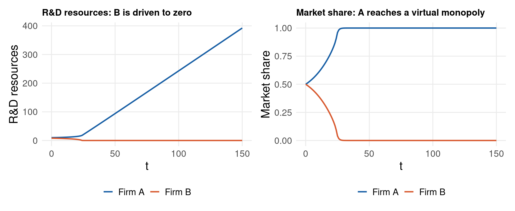
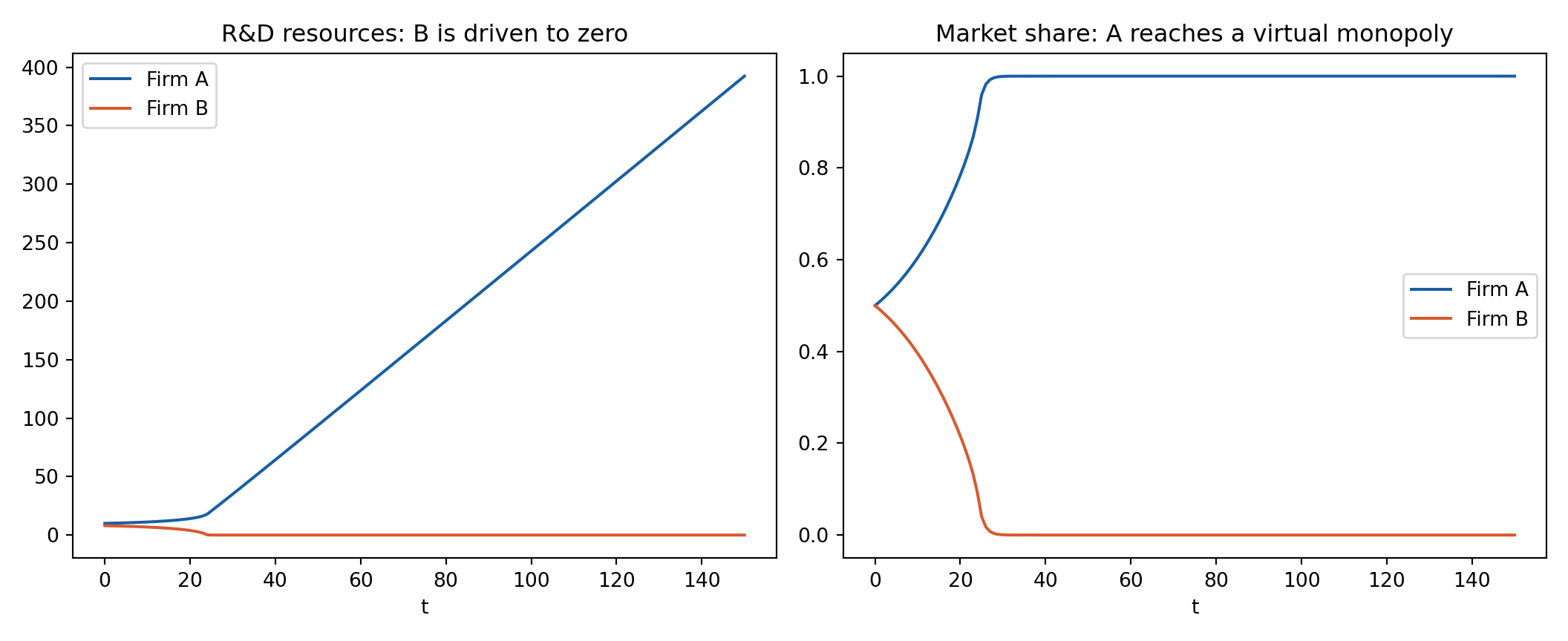
Example 9.1 (Shone): both firms reinforce (\(a,b>0\)), starting from a small resource head-start for firm \(A\): \(R^A_0=10 > R^B_0=8\), \(m^A=m^B=100\), \(n^A=n^B=40\), equal initial market shares \(k^A_0=k^B_0=0.5\), share-adjustment speed \(\gamma=0.01\).
With both firms reinforcing, whichever firm starts even slightly ahead in quality keeps widening its lead: a higher \(S^A_t\) raises \(R^A_{t+1}\) (reinforcing), which raises \(S^A_{t+1}\) further, while the same gap simultaneously shrinks firm \(B\)’s reinforcement term \(b(S^B_t-S^A_t)<0\). This is a self-reinforcing (positive-feedback) mechanism with no counteracting force — Shone’s simulation shows firm \(A\)’s market share converging to \(1\) and firm \(B\)’s R&D resources being driven to (and held at) zero.
\[\boxed{\text{Both reinforcing} \;\Rightarrow\; k^A_t \to 1,\; k^B_t \to 0 \;\Rightarrow\; \text{firm B exits the market}}\]
Only a symmetric start (\(R^A_0=R^B_0\)) avoids this outcome — any asymmetry, however small, is amplified over time.
Simulating market dominance under mutual reinforcement:
For each period \(t\): compute quality standards \(S^A_t, S^B_t\) (floored at zero, matching Shone’s spreadsheet constraint), then the industry average \(\bar S_t = k^A_tS^A_t+k^B_tS^B_t\)
Substituting the quality equations into the resource equations gives a genuinely nonlinear two-dimensional map \(R^i_{t+1} = f^i(R^A_t, R^B_t)\) — the \(\arctan\) term rules out any closed-form solution of the kind used throughout this chapter (no eigenvalues, no explicit \(\lambda^t\) terms).
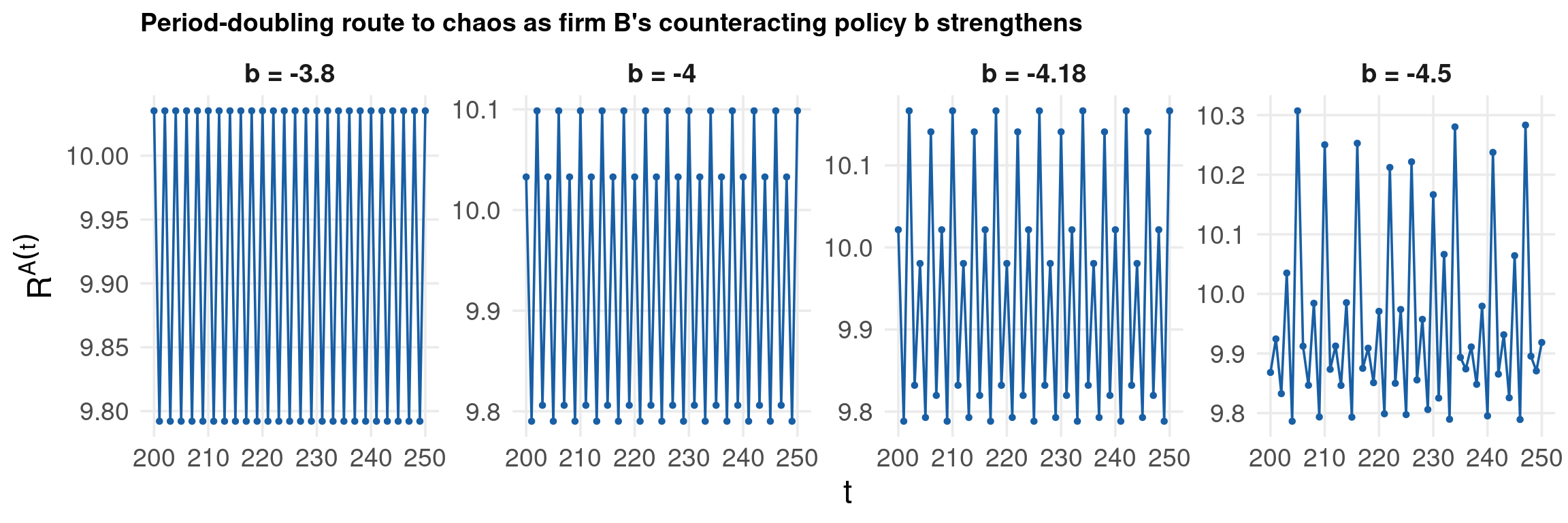
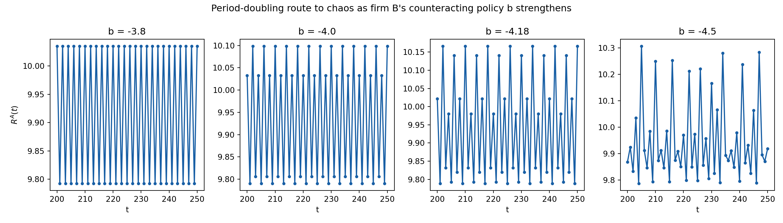
If one firm reinforces while the other counteracts (mixed policy, e.g. \(a>0, b<0\)), the system has no fixed steady state to converge to: it settles into a limit cycle or wanders chaotically instead. Holding \(a=0.1\) fixed and varying \(b\) traces out a period-doubling route to chaos — exactly the same qualitative route as the logistic map \(x_{t+1}=\lambda x_t(1-x_t)\) (Parts III & VII of the theory deck), but generated here by an economic mechanism (competing R&D policies) rather than a population-growth equation:
Every model earlier in this chapter was linear, so instability always meant monotone or oscillatory divergence to \(\pm\infty\). Here, the nonlinearity (\(\arctan\) is bounded and the \(\max[0,\cdot]\) clips at zero) keeps trajectories bounded even when they never settle down — the hallmark of deterministic chaos rather than simple explosive instability.
Simulating the R&D competition and revealing the period-doubling cascade:
For each candidate value of firm \(B\)’s policy \(b \in \{-3.8,\,-4.0,\,-4.18,\,-4.5\}\) (all counteracting, \(b<0\)):
Iterate the two-equation map for \(T_{\max}=250\) periods: at each \(t\) compute \(S^A_t, S^B_t\) from the current resources, then update \(R^A_{t+1}, R^B_{t+1}\) via the \(\max[0,\cdot]\) rule
Discard the transient: keep only \(t=200,\dots,250\), since the interesting long-run behaviour only emerges after the initial adjustment dies out
Plot \(R^A_t\) against \(t\) over the retained window, one panel per \(b\)
Read the qualitative regime directly off the shape: a clean up-down zig-zag (period-2), a slower-repeating wiggle (period-4 or higher), or a trace that never repeats (chaos) — precisely as with the logistic-map bifurcation cascade
Code
simulate_rd <-function(a, b, mA =100, mB =100, nA =40, nB =40,RA0 =10, RB0 =15, Tmax =250) { RA <-numeric(Tmax +1); RB <-numeric(Tmax +1) RA[1] <- RA0; RB[1] <- RB0for (t inseq_len(Tmax)) { SA <- (2* mA / pi) *atan(RA[t]) - nA SB <- (2* mB / pi) *atan(RB[t]) - nB RA[t +1] <-max(0, RA[t] + a * (SA - SB)) RB[t +1] <-max(0, RB[t] + b * (SB - SA)) }tibble(t =0:Tmax, RA = RA, RB = RB)}bs <-c(-3.8, -4.0, -4.18, -4.5)df_rd <-tibble()for (b in bs) { df_b <-simulate_rd(a =0.1, b = b) %>%filter(t >=200, t <=250) %>%mutate(b =glue("b = {b}")) df_rd <-bind_rows(df_rd, df_b)}ggplot(df_rd) +aes(x = t, y = RA) +geom_line(color ="#185FA5") +geom_point(color ="#185FA5", size =1) +facet_wrap(~b, scales ="free_y", nrow =1) +labs(x ="t", y =expression(R^A(t)),title ="Period-doubling route to chaos as firm B's counteracting policy b strengthens") + theme_lecture
Code
import numpy as npimport matplotlib.pyplot as pltdef simulate_rd(a, b, mA=100, mB=100, nA=40, nB=40, RA0=10.0, RB0=15.0, Tmax=250): RA = np.zeros(Tmax +1); RB = np.zeros(Tmax +1) RA[0], RB[0] = RA0, RB0for t inrange(Tmax): SA = (2*mA/np.pi)*np.arctan(RA[t]) - nA SB = (2*mB/np.pi)*np.arctan(RB[t]) - nB RA[t +1] =max(0, RA[t] + a*(SA - SB)) RB[t +1] =max(0, RB[t] + b*(SB - SA))return RA, RBbs = [-3.8, -4.0, -4.18, -4.5]fig, axes = plt.subplots(1, 4, figsize=(14, 4))t_full = np.arange(251)mask = (t_full >=200) & (t_full <=250)for ax, b inzip(axes, bs): RA, RB = simulate_rd(0.1, b) ax.plot(t_full[mask], RA[mask], marker="o", markersize=3, color="#185FA5") ax.set_title(f"b = {b}"); ax.set_xlabel("t")axes[0].set_ylabel(r"$R^A(t)$")fig.suptitle("Period-doubling route to chaos as firm B's counteracting policy b strengthens")plt.tight_layout(); plt.show()
Shone’s §9.5.2 lets the policy parameters \(a, b\) themselves adapt. Every \(f\) periods, each firm reviews its recent relative performance:
\[M = \sum_{s=t-f+1}^{t}\big(S^A_s - S^B_s\big)\]
Since a positive \(M\) for firm \(A\) implies a negative \(M\) for firm \(B\) (and vice versa), exactly one firm revises its policy at each decision point — the one that has been losing ground. Two adaptation rules:
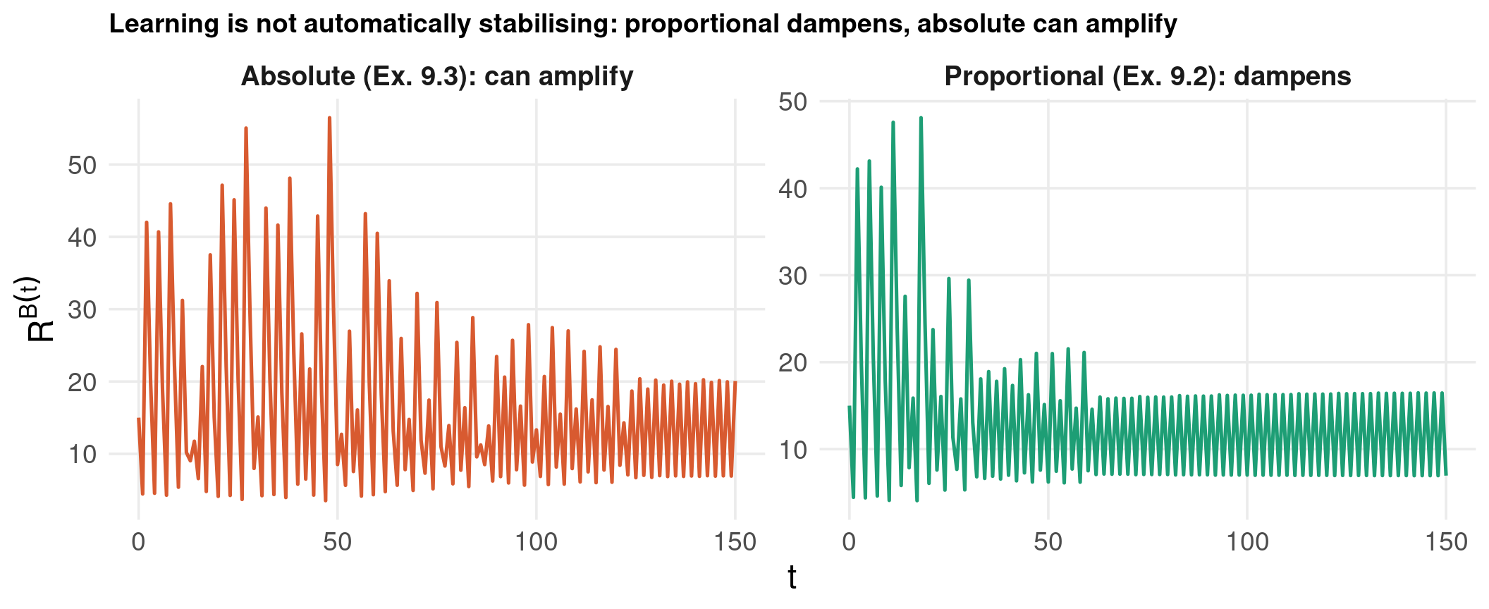
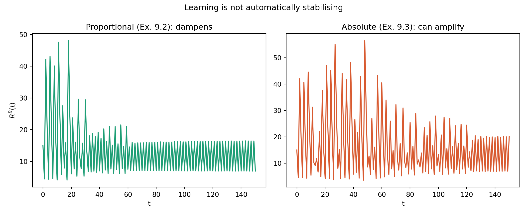
Proportional adaptation only dampens the existing stance (reinforcing stays reinforcing, just weaker); absolute adaptation can flip its sign entirely, turning a reinforcing policy counteracting or vice versa.
Example 9.2 (proportional):\(m^A=m^B=100\), \(n^A=n^B=40\), \(\alpha=0.8\), \(\beta=0.9\), \(a_0=0.1\), \(b_0=-5.0\), \(f=10\). After an early erratic period, the system settles down: each policy revision shrinks \(|a|\) and \(|b|\) a little further, so the oscillation amplitude shrinks in stages.
Example 9.3 (absolute):\(\alpha=-0.05\), \(\beta=0.2\), \(a_0=0.13\), \(b_0=-5.0\), \(f=10\) (otherwise identical). Here adaptation can overshoot past zero and reverse the policy’s sign at an unlucky moment — Shone finds the resource path becomes more erratic over time, not less.
\[\boxed{\text{Learning is not automatically stabilising — it depends entirely on } \textit{how} \text{ the policy adapts}}\]
Simulating both adaptation rules side by side:
Run the base R&D recursion (as in the previous slide) but track a current policy pair \((a_s, b_s)\) that starts at \((a_0, b_0)\)
Every \(f=10\) periods, compute \(M=\sum(S^A-S^B)\) over the just-completed window
If \(M<0\): revise firm \(A\)’s policy; if \(M>0\): revise firm \(B\)’s policy — proportionally (\(a_s=\alpha a_{s-1}\)) or absolutely (\(a_s=a_{s-1}+\alpha\)), depending on which example is being run
Iterate \(T=150\) periods for each rule and plot \(R^B_t\) (the series where the contrast is clearest) — proportional adaptation should visibly narrow its swings over time; absolute adaptation should widen them
Code
simulate_learning <-function(a0, b0, alpha, beta, mode =c("proportional", "absolute"),mA =100, mB =100, nA =40, nB =40,RA0 =10, RB0 =15, f =10, Tmax =150) { mode <-match.arg(mode) RA <-numeric(Tmax +1); RB <-numeric(Tmax +1) RA[1] <- RA0; RB[1] <- RB0 a_cur <- a0; b_cur <- b0 SA_hist <-numeric(Tmax +1); SB_hist <-numeric(Tmax +1)for (t inseq_len(Tmax)) { SA <- (2* mA / pi) *atan(RA[t]) - nA SB <- (2* mB / pi) *atan(RB[t]) - nB SA_hist[t] <- SA; SB_hist[t] <- SB RA[t +1] <-max(0, RA[t] + a_cur * (SA - SB)) RB[t +1] <-max(0, RB[t] + b_cur * (SB - SA))if (t %% f ==0) { # decision point every f periods M <-sum(SA_hist[max(1, t - f +1):t] - SB_hist[max(1, t - f +1):t])if (M <0) { # firm A has been losing ground a_cur <-if (mode =="proportional") alpha * a_cur else a_cur + alpha } elseif (M >0) { # firm B has been losing ground b_cur <-if (mode =="proportional") beta * b_cur else b_cur + beta } } }tibble(t =0:Tmax, RA = RA, RB = RB)}df_prop <-simulate_learning(a0 =0.1, b0 =-5.0, alpha =0.8, beta =0.9, mode ="proportional") %>%mutate(rule ="Proportional (Ex. 9.2): dampens")df_abs <-simulate_learning(a0 =0.13, b0 =-5.0, alpha =-0.05, beta =0.2, mode ="absolute") %>%mutate(rule ="Absolute (Ex. 9.3): can amplify")df_learn <-bind_rows(df_prop, df_abs)ggplot(df_learn) +aes(x = t, y = RB, color = rule) +geom_line(linewidth =0.9) +facet_wrap(~rule, scales ="free_y") +scale_color_manual(values =c("Proportional (Ex. 9.2): dampens"="#1D9E75","Absolute (Ex. 9.3): can amplify"="#D85A30"), guide ="none") +labs(x ="t", y =expression(R^B(t)),title ="Learning is not automatically stabilising: proportional dampens, absolute can amplify") + theme_lecture
Code
import numpy as npimport matplotlib.pyplot as pltdef simulate_learning(a0, b0, alpha, beta, mode="proportional", mA=100, mB=100, nA=40, nB=40, RA0=10.0, RB0=15.0, f=10, Tmax=150): RA = np.zeros(Tmax +1); RB = np.zeros(Tmax +1) RA[0], RB[0] = RA0, RB0 a_cur, b_cur = a0, b0 SA_hist = np.zeros(Tmax +1); SB_hist = np.zeros(Tmax +1)for t inrange(1, Tmax +1): SA = (2*mA/np.pi)*np.arctan(RA[t-1]) - nA SB = (2*mB/np.pi)*np.arctan(RB[t-1]) - nB SA_hist[t-1], SB_hist[t-1] = SA, SB RA[t] =max(0, RA[t-1] + a_cur*(SA - SB)) RB[t] =max(0, RB[t-1] + b_cur*(SB - SA))if t % f ==0: M = np.sum(SA_hist[max(0, t-f):t] - SB_hist[max(0, t-f):t])if M <0: a_cur = alpha*a_cur if mode =="proportional"else a_cur + alphaelif M >0: b_cur = beta*b_cur if mode =="proportional"else b_cur + betareturn RA, RBRA_p, RB_p = simulate_learning(0.1, -5.0, 0.8, 0.9, mode="proportional")RA_a, RB_a = simulate_learning(0.13, -5.0, -0.05, 0.2, mode="absolute")t = np.arange(151)fig, axes = plt.subplots(1, 2, figsize=(11, 4.5))axes[0].plot(t, RB_p, color="#1D9E75")axes[0].set_title("Proportional (Ex. 9.2): dampens"); axes[0].set_xlabel("t"); axes[0].set_ylabel(r"$R^B(t)$")axes[1].plot(t, RB_a, color="#D85A30")axes[1].set_title("Absolute (Ex. 9.3): can amplify"); axes[1].set_xlabel("t")fig.suptitle("Learning is not automatically stabilising")plt.tight_layout(); plt.show()
Extension II — Schumpeterian Selection & Imitation (§9.6)
A different evolutionary story: instead of quantities or R&D budgets, firms’ market shares evolve according to relative profitability. Firm \(i\) has unit cost \(c^i_t\), faces a common price \(p\), so its profit margin is \(\pi^i_t = p - c^i_t\). Given market shares \(k^i_t\) (with \(\sum_i k^i_t=1\)), the share-weighted industry average margin is
\[\bar\pi_t = \sum_i k^i_t\, \pi^i_t\]
Selection: a firm’s percentage change in market share is proportional to how far its margin is above or below the industry average:
(the \(\max[\cdot,0]\) and renormalisation keep shares non-negative and summing to 1 for any number of firms). Imitation: laggards close part of the cost gap to the most efficient firm in the industry, \(c^{\min}_t=\min_i c^i_t\):
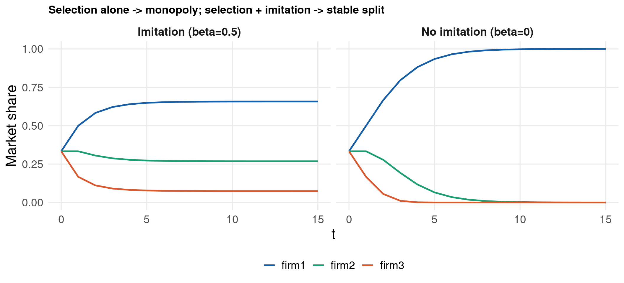
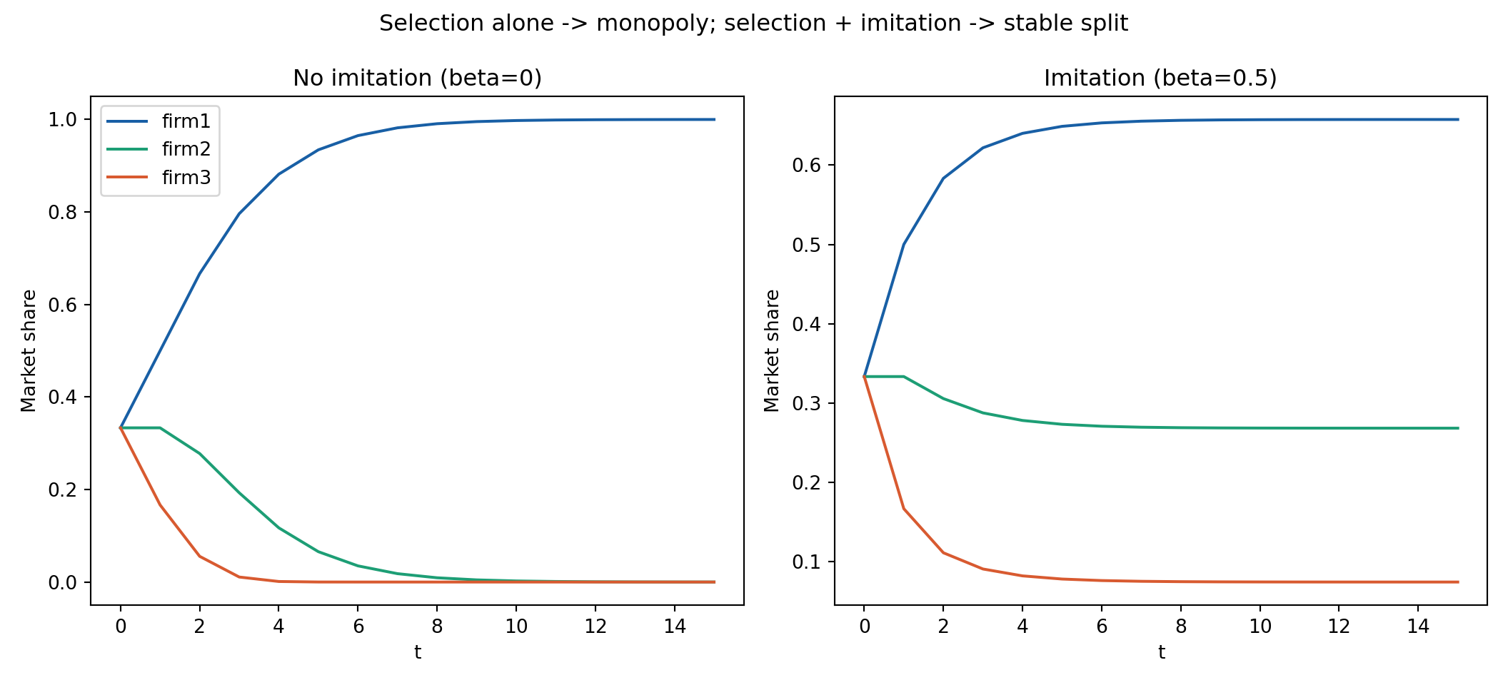
With no imitation (\(\beta=0\)), a fixed cost advantage is self-reinforcing: the low-cost firm’s margin stays above average every period, so \(\hat k^i_t>0\) compounds and its share is driven toward \(1\) — survival of the fittest, ending in a near-monopoly.
With imitation (\(\beta>0\)), laggards’ costs are pulled toward \(c^{\min}_t\) each period, shrinking the margin gap that selection feeds on. The market settles into an interior distribution that reflects the initial cost advantage rather than collapsing to a corner. For \(c_0=(8,10,12)\), \(p=18\), \(\alpha=0.25\):
Unlike every model earlier in this chapter, there is no oscillation possible here at all: \(\alpha,\beta>0\) means selection always reallocates share toward current winners and imitation always pulls costs toward the current leader — both forces are one-directional, so the only long-run possibilities are convergence to a monopoly or to a stable interior mix, never a cycle.
Simulating selection-and-imitation dynamics:
Initialise \(n\) firms’ unit costs \(c^i_0\) and market shares \(k^i_0\) (summing to 1); fix the common price \(p\) and parameters \(\alpha,\beta\)
For each period \(t=1,\dots,T\):
Compute each firm’s margin \(\pi^i_t = p - c^i_t\) and the share-weighted industry average \(\bar\pi_t\)
Compute the raw share growth rate \(\hat k^i_t = \alpha(\pi^i_t-\bar\pi_t)\), apply it multiplicatively to last period’s share, clip at zero, then renormalise so shares sum to 1
Pull each firm’s cost toward the industry’s current minimum: \(c^i_{t+1} = c^i_t-\beta(c^i_t-c^{\min}_t)\)
Repeat for \(T\) periods and record the path of \(k^i_t\) and \(c^i_t\)
Re-run the whole simulation twice — once with \(\beta=0\), once with \(\beta=0.5\) — holding \(\alpha\), \(c_0\), \(k_0\) fixed, to isolate the effect of imitation
Plot market shares over time for both runs side by side: one should collapse to a corner, the other to a stable interior split
Code
simulate_schumpeter <-function(costs0, shares0, price, alpha, beta, T =15) { n <-length(costs0) C <-matrix(0, T +1, n); K <-matrix(0, T +1, n) C[1, ] <- costs0; K[1, ] <- shares0for (t inseq_len(T)) { c <- C[t, ]; k <- K[t, ] margin <- price - c avg_margin <-sum(k * margin) khat <- alpha * (margin - avg_margin) k_raw <-pmax(k * (1+ khat), 0) K[t +1, ] <- k_raw /sum(k_raw) # renormalise to sum to 1 C[t +1, ] <- c - beta * (c -min(c)) # imitate the cheapest firm }tibble(t =0:T, firm1 = K[, 1], firm2 = K[, 2], firm3 = K[, 3])}df_no_imit <-simulate_schumpeter(c(8, 10, 12), rep(1/3, 3), price =18, alpha =0.25, beta =0) %>%pivot_longer(-t, names_to ="firm", values_to ="share") %>%mutate(regime ="No imitation (beta=0)")df_imit <-simulate_schumpeter(c(8, 10, 12), rep(1/3, 3), price =18, alpha =0.25, beta =0.5) %>%pivot_longer(-t, names_to ="firm", values_to ="share") %>%mutate(regime ="Imitation (beta=0.5)")ggplot(bind_rows(df_no_imit, df_imit)) +aes(x = t, y = share, color = firm) +geom_line(linewidth =1) +facet_wrap(~regime) +scale_color_manual(values =c("#185FA5", "#1D9E75", "#D85A30"), name =NULL) +labs(x ="t", y ="Market share",title ="Selection alone -> monopoly; selection + imitation -> stable split") + theme_lecture
Replace quantity competition with price competition on a differentiated good, following the linear demand system of Singh & Vives (1984). Demand for firm \(i\) rises in its rivals’ prices (substitutes) and falls in its own:
This is the key structural difference from Cournot, in the terminology of Bulow, Geanakoplos & Klemperer (1985): the Cournot reaction function has slope \(-\tfrac12\) (quantities are strategic substitutes — if my rival produces more, I produce less). The Bertrand reaction function here has slope \(+r\) (prices are strategic complements — if my rival raises its price, I raise mine too, since my good looks relatively cheaper otherwise).
Exactly the same \(J\)-matrix algebra as the Theocharis theorem applies, with \(-\tfrac12\) replaced by \(+r\): for \(n\) symmetric firms, \(\mathbf{p}_t = \text{intercept}\cdot\mathbf{1} + r(J-I)\mathbf{p}_{t-1}\), eigenvalues
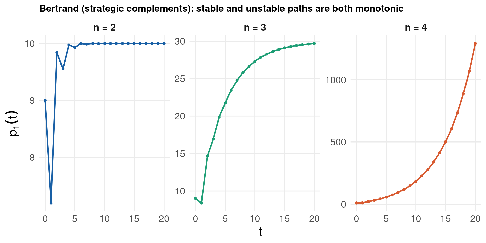
Stability again requires \(|\lambda_1|<1 \iff r(n-1)<1\) — algebraically the same threshold shape as Theocharis. But now \(\lambda_1\) is positive rather than negative. The symmetric mode \(\lambda_1=r(n-1)\) grows with \(n\) while the antisymmetric mode \(\lambda_2=-r\) stays fixed, so as \(n\) increases the positive symmetric mode increasingly dominates the trajectory: for \(n\geq 3\) the path is essentially monotonic, and crossing the threshold produces monotonic, ever-increasing prices (an industry-wide “price bubble”) rather than an alternating spiral. With \(a=9,b=1,c=3,d=0.8\Rightarrow r=0.4\): intercept \(=6\), so \(q_i^*=6/(1-0.4(n-1))\).
What about duopoly (n=2)?
For \(n=2\) specifically, both eigenvalues \(\lambda_1=r\) and \(\lambda_2=-r\) have the same multiplicity (one each), so an asymmetric starting point (e.g. one firm’s price far above the other’s) still excites the negative antisymmetric mode and produces a transient overshoot before settling — visible as a brief dip in the code output below. This is the one case where “strategic complements ⇒ purely monotonic” does not strictly hold; the clean dichotomy with Cournot only fully emerges once \(n\geq3\), where the growing symmetric eigenvalue \(r(n-1)\) dominates.
For Cournot (strategic substitutes), continuous-time adjustment \(\dot q_i=k(x_i-q_i)\) was unconditionally stable for any \(n\) (all eigenvalues of the Jacobian negative regardless of \(n\)). For Bertrand (strategic complements), the same derivation gives Jacobian eigenvalue \(k\big(1-r(n-1)\big)\) on the symmetric mode — positive (unstable) whenever \(r(n-1)>1\), exactly the same threshold as the discrete case. Verified numerically: with \(r=0.4\), continuous-time prices converge for \(n=2,3\) but diverge monotonically for \(n=4\). The sign of the reaction-function slope, not just its magnitude, determines whether continuous time is a stabilising force.
Step 0 — compute the Bertrand equilibrium for any \(n\) by solving, not guessing: the fixed point solves \(\big(I-r(J-I)\big)\mathbf{p}^*=\text{intercept}\cdot\mathbf{1}\) — the same linear-solver pattern as Cournot, just with \(-r\) in place of \(+\tfrac12\) (or \(+\tfrac18\)). We verify \(p^*=6/(1-0.4(n-1))\) this way for \(n=2,3\) before simulating.
Adapting the Theocharis comparison to price competition:
Reuse the exact structure of simulate_discrete(), but replace the Cournot reaction function (\(3 - \tfrac12\,\text{rival\_sum}\)) with the Bertrand one (\(6 + 0.4\,\text{rival\_sum}\)) — same loop, same bookkeeping, only the sign and the coefficient change
For each \(n \in \{2,3,4\}\), start firm 1 “high” (e.g. \(p_1=9\)) and the rest “low” (\(p_j=3\)), and iterate \(T=20\) periods
Plot firm 1’s price path per \(n\) on separate y-axes (facets), exactly as in the Theocharis slide
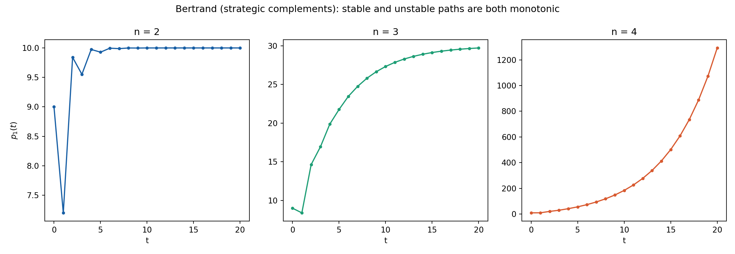
Compare shapes directly against the earlier Cournot comparison figure: the \(n=2\) panel shows a brief overshoot (both eigenvalues \(\pm r\) have equal weight for duopoly), but \(n=3\) and \(n=4\) are cleanly monotonic — steadily rising toward the fixed point or steadily exploding — with no zig-zag at all, unlike the Cournot \(n=3,4\) paths which alternate
Code
# Step 0: solve the Bertrand equilibrium directly (any n), then check against the closed formbertrand_equilibrium <-function(n, r =0.4, intercept =6) { J <-matrix(1, n, n); I <-diag(n)solve(I - r * (J - I), rep(intercept, n))}for (n in2:3) {cat("n =", n, " solved p* =", round(bertrand_equilibrium(n)[1], 4)," | formula intercept/(1-r(n-1)) =", round(6/ (1-0.4* (n -1)), 4), "\n")}simulate_bertrand <-function(n, T, p0, r =0.4, intercept =6) { p <-matrix(0, T +1, n); p[1, ] <- p0for (t inseq_len(T)) { prev <- p[t, ]for (i inseq_len(n)) { rival_sum <-sum(prev[-i]) p[t +1, i] <- intercept + r * rival_sum # positive slope: strategic complements } } p}df_bertrand <-tibble()for (n in2:4) { res <-simulate_bertrand(n, 20, p0 =c(9, rep(3, n -1))) df_this_n <-tibble(t =0:20, p1 = res[, 1], n =glue("n = {n}")) df_bertrand <-bind_rows(df_bertrand, df_this_n)}ggplot(df_bertrand) +aes(x = t, y = p1, color = n) +geom_line(linewidth =1) +geom_point(size =1.2) +facet_wrap(~n, scales ="free_y", nrow =1) +scale_color_manual(values =c("#185FA5", "#1D9E75", "#D85A30"), name =NULL, guide ="none") +labs(x ="t", y =expression(p[1](t)),title ="Bertrand (strategic complements): stable and unstable paths are both monotonic") + theme_lecture
# A tibble: 2 × 3
      n solved formula
  <int>  <dbl>   <dbl>
1     2     10      10
2     3     30      30
Code
import numpy as npimport matplotlib.pyplot as plt# Step 0: solve the Bertrand equilibrium directly (any n), then check against the closed formdef bertrand_equilibrium(n, r=0.4, intercept=6.0): J = np.ones((n, n)); I = np.eye(n)return np.linalg.solve(I - r * (J - I), np.full(n, intercept))for n in [2, 3]: solved = bertrand_equilibrium(n)[0]print(f"n={n} solved p*={solved:.4f} formula intercept/(1-r(n-1))={6/(1-0.4*(n-1)):.4f}")
n=2  solved p*=10.0000  formula intercept/(1-r(n-1))=10.0000
n=3  solved p*=30.0000  formula intercept/(1-r(n-1))=30.0000
Code
def simulate_bertrand(n, T, p0, r=0.4, intercept=6.0): p = np.zeros((T +1, n)); p[0] = p0for t inrange(T): prev = p[t].copy()for i inrange(n): rival_sum = prev.sum() - prev[i] p[t +1, i] = intercept + r * rival_sumreturn pfig, axes = plt.subplots(1, 3, figsize=(13, 4.5))colors = {2: "#185FA5", 3: "#1D9E75", 4: "#D85A30"}for ax, n inzip(axes, [2, 3, 4]): p0 = np.array([9.0] + [3.0]*(n -1)) res = simulate_bertrand(n, 20, p0) ax.plot(range(21), res[:, 0], color=colors[n], marker="o", markersize=3) ax.set_title(f"n = {n}"); ax.set_xlabel("t")axes[0].set_ylabel(r"$p_1(t)$")fig.suptitle("Bertrand (strategic complements): stable and unstable paths are both monotonic")plt.tight_layout(); plt.show()
Return to the baseline duopoly (\(p=9-Q\), \(TC_i=3q_i\)). The Cournot-Nash equilibrium \((2,2)\) is not what maximises the firms’ joint profit. Joint profit maximisation solves
Collusion raises price (\(p=6\) vs. \(p=5\)) and raises joint profit (\(\Pi^c=9\) vs. \(\Pi^{CN}=8\)) by restricting output below the competitive level — the same conclusion as the static duopoly slide, now made dynamic.
Model tacit collusion as a blend: each firm targets a weighted average of its Cournot best response to the rival’s last output and the collusive output, with \(\omega\in[0,1]\) indexing the degree of collusion:
This \(\omega\) is a reduced-form stylisation, not a derived equilibrium object: the rigorous game-theoretic foundation for sustaining \((1.5,1.5)\) as a non-cooperative equilibrium is Friedman’s (1971) trigger-strategy supergame — firms collude as long as both comply, and revert permanently to the (worse, but still self-enforcing) Cournot-Nash punishment the moment either firm deviates. \(\omega\) can be read informally as indexing how close discount factors and detection lags are to sustaining that trigger strategy, without solving the repeated game explicitly.
Since the collusive term is a constant (independent of the rival’s output), it shifts only the intercept, not the matrix — the dynamic system is still \(\mathbf{q}_t = \mathbf{a}(\omega) + (1-\omega)B\,\mathbf{q}_{t-1}\) with the same\(B\) as the pure-Cournot case. Eigenvalues shrink uniformly toward zero:
The blended system is stable for every degree of collusion — more collusion never destabilises it, and in fact speeds up convergence (smaller \(|\lambda|\)). Solving for the fixed point:
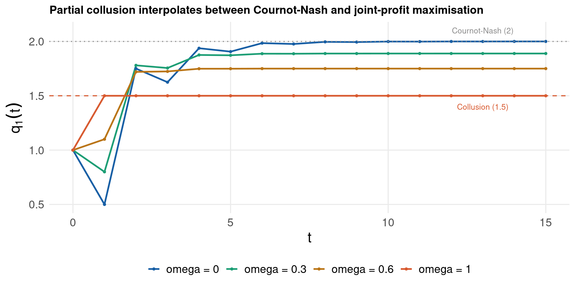
As \(\omega\) rises from 0 to 1, the long-run output smoothly interpolates between the competitive and the collusive outcome — a stylised way of asking “how close to collusion does partial cooperation get us?”
Step 0 — compute both reference points with a solver, not by hand: the Cournot-Nash point reuses the linear solver from the very first duopoly slide (solve() on the two FOCs); the collusive output requires a genuinely different tool — a one-dimensional optimiser (optimize(..., maximum=TRUE) in R, scipy.optimize.minimize_scalar in Python) applied to the joint-profit function \(\Pi(Q)=(9-Q)Q-3Q\), since maximising a sum of profits is not itself a fixed point of any reaction function.
Simulating partial collusion — blending two targets each period:
Solve for the two reference points as above: \(q^{CN}=2\) (linear solve) and \(q^c=1.5\) (scalar optimisation)
Fix an initial condition, e.g. \((q_{1,0},q_{2,0})=(1,5)\)
For each candidate degree of collusion \(\omega \in \{0,\,0.3,\,0.6,\,1\}\):
At each period, compute the ordinary Cournot best response to the rival’s lagged output, then blend it with the fixed collusive target \(1.5\) using weight \(\omega\)
Set this period’s output equal to the blended target (complete adjustment, as in the very first duopoly slide)
Collect all four trajectories and plot them on one panel together with horizontal reference lines at \(q^{CN}=2\) and \(q^c=1.5\)
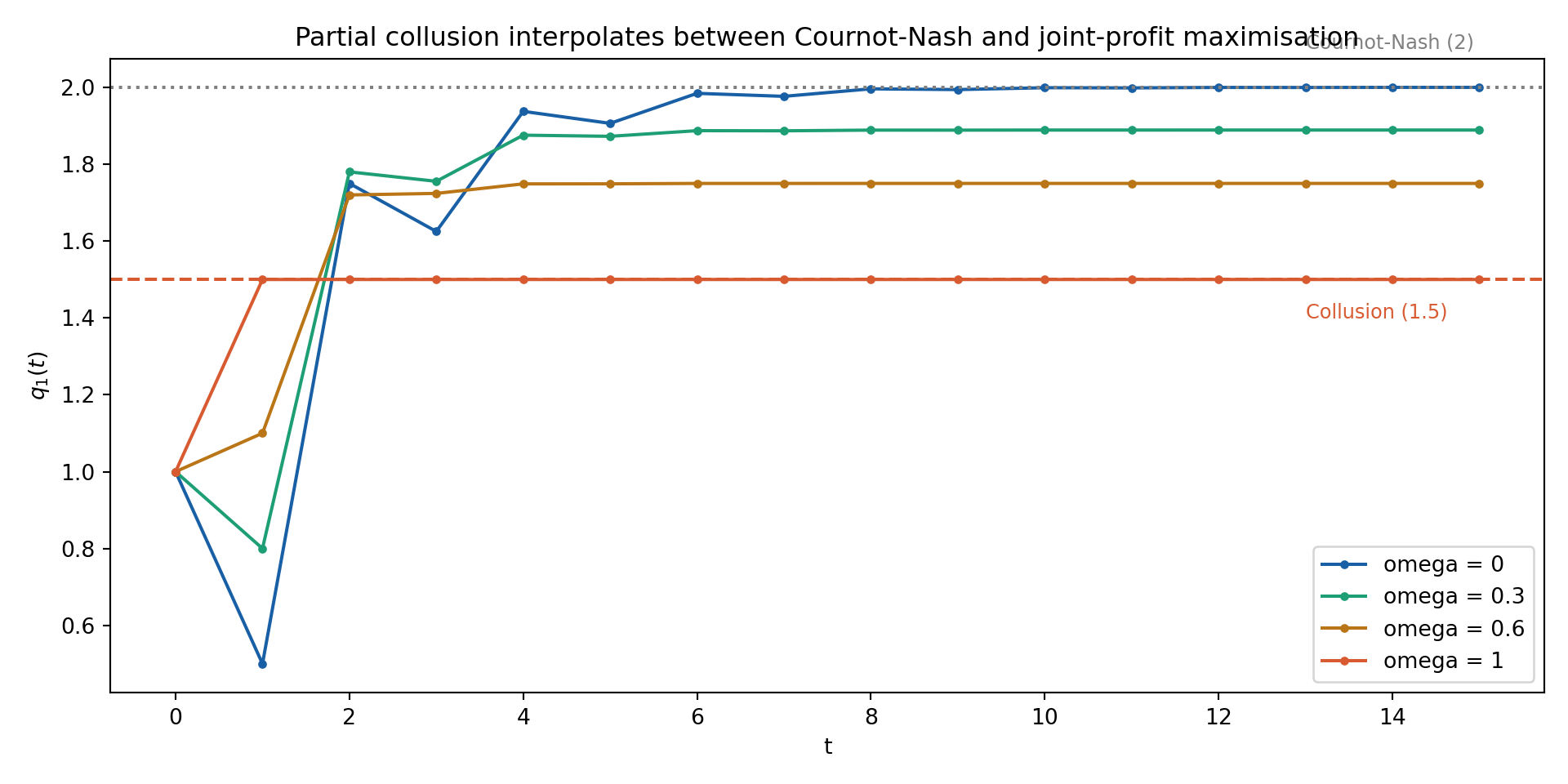
Confirm: every path is stable regardless of \(\omega\), and higher \(\omega\) visibly pulls the long-run level down from 2 toward 1.5 while also converging faster
Code
# Step 0: solve for both reference points instead of quoting them from the theory slideq_cournot <-solve(matrix(c(2, 1, 1, 2), nrow =2), c(6, 6))[1] # linear solve, as beforejoint_profit <-function(Q) (9- Q) * Q -3* Q # Pi(Q), not a firm's own profitopt <-optimize(joint_profit, interval =c(0, 9), maximum =TRUE)q_collusive <- opt$maximum /2# split the optimal Q equallycat("Cournot-Nash q* =", q_cournot, " | Collusive q^c =", q_collusive, "\n")simulate_collusion <-function(omega, T, q0, qc =1.5) { q <-matrix(0, T +1, 2); q[1, ] <- q0for (t inseq_len(T)) { prev <- q[t, ] x1 <- (1- omega) * (3-0.5* prev[2]) + omega * qc x2 <- (1- omega) * (3-0.5* prev[1]) + omega * qc q[t +1, ] <-c(x1, x2) } q}omegas <-c(0, 0.3, 0.6, 1)df_coll <-tibble()for (om in omegas) { res <-simulate_collusion(om, 15, q0 =c(1, 5)) df_this_om <-tibble(t =0:15, q1 = res[, 1], omega =glue("omega = {om}")) df_coll <-bind_rows(df_coll, df_this_om)}ggplot(df_coll) +aes(x = t, y = q1, color = omega) +geom_line(linewidth =1) +geom_point(size =1) +geom_hline(yintercept =2, linetype ="dotted", color ="grey55") +geom_hline(yintercept =1.5, linetype ="dashed", color ="#D85A30") +annotate("text", x =13, y =2.1, label ="Cournot-Nash (2)", color ="grey55", size =3.5) +annotate("text", x =13, y =1.4, label ="Collusion (1.5)", color ="#D85A30", size =3.5) +scale_color_manual(values =c("#185FA5", "#1D9E75", "#BA7517", "#D85A30"), name =NULL) +labs(x ="t", y =expression(q[1](t)),title ="Partial collusion interpolates between Cournot-Nash and joint-profit maximisation") + theme_lecture
Cournot-Nash q* = 2 | Collusive q^c = 1.5
Code
import numpy as npfrom scipy.optimize import minimize_scalarimport matplotlib.pyplot as plt# Step 0: solve for both reference points instead of quoting them from the theory slideq_cournot = np.linalg.solve(np.array([[2, 1], [1, 2]]), np.array([6, 6]))[0]joint_profit =lambda Q: -((9- Q) * Q -3* Q) # negate: minimize_scalar finds a minimumopt = minimize_scalar(joint_profit, bounds=(0, 9), method="bounded")q_collusive = opt.x /2print(f"Cournot-Nash q* = {q_cournot:.4f} | Collusive q^c = {q_collusive:.4f}")
For \(p = A - BQ\), \(TC_i = a_iq_i\), \(n\) firms, show that the reaction functions are \(q_i = \dfrac{(A-a_i) - B\sum_{j\neq i}q_j}{2B}\), that \(q_i^*\) collapses to a common value when all \(a_i\) are equal, and re-derive the Theocharis threshold \(n<3\) for general \(A, B\) (it should not depend on \(A\) or \(B\) at all).
Re-run the discrete \(n=2\) constant-MC simulation with \(TC_1 = 3q_1\), \(TC_2 = 5q_2\) (asymmetric costs). Does the equilibrium still satisfy \(q_1^* > q_2^*\)? Does convergence still hold?
Set \(k = k^*(n) = 4/(n+1)\) exactly for \(n=3\) and confirm numerically that the system enters an undamped two-period oscillation, as predicted by \(\mu_1 = -1\).
Extend the continuous-time R code to \(n=5\) and \(n=6\) firms and confirm that the equilibrium remains a stable node in every case, even though \(\det(-A)\) alternates in sign.
Part II: Dynamics of Inflation and Unemployment
Shone, Ch. 11 — the expectations-augmented Phillips curve
Literature Review — Part II: Inflation & Unemployment Dynamics
Phillips, A. W. (1958). The relation between unemployment and the rate of change of money wage rates in the United Kingdom, 1861–1957. Economica, 25(100), 283–299. DOI: 10.2307/2550759
Phelps, E. S. (1967). Phillips curves, expectations of inflation and optimal unemployment over time. Economica, 34(135), 254–281. DOI: 10.2307/2552025
Friedman, M. (1968). The role of monetary policy. American Economic Review, 58(1), 1–17. JSTOR
Cagan, P. (1956). The monetary dynamics of hyperinflation. In M. Friedman (Ed.), Studies in the Quantity Theory of Money (pp. 25–117). University of Chicago Press.
Lucas, R. E. (1972). Expectations and the neutrality of money. Journal of Economic Theory, 4(2), 103–124. DOI: 10.1016/0022-0531(72)90142-1
Sargent, T. J., & Wallace, N. (1975). “Rational” expectations, the optimal monetary instrument, and the optimal money supply rule. Journal of Political Economy, 83(2), 241–254. DOI: 10.1086/260321
Groth, C. (1993). Some unfamiliar dynamics of a familiar macro model: a note. Journal of Economics, 58(3), 293–305. DOI: 10.1007/BF01235251
McCafferty, S. (1990). Macroeconomic Theory. Harper & Row.
Azariadis, C. (1993). Intertemporal Macroeconomics. Blackwell.
Burmeister, E., & Dobell, A. R. (1970). Mathematical Theories of Economic Growth. Macmillan.
George, D. A. R., & Oxley, L. (1991). Fixed money growth rules and the rate of inflation: global versus local dynamics. Scottish Journal of Political Economy, 38(3), 209–226. DOI: 10.1111/j.1467-9485.1991.tb00312.x
Turnovsky, S. J. (1995). Methods of Macroeconomic Dynamics. MIT Press.
The Inflation-Unemployment Problem
Original Phillips curve: an empirical negative relationship between wage inflation and unemployment
Problem: the relationship broke down in the 1970s (stagflation — high inflation and high unemployment together)
Resolution: expectations of inflation matter, not just the unemployment rate — this is exactly the kind of backward-looking dynamic adjustment studied throughout this course
Following Shone (2002, Ch. 11), we work through the expectations-augmented Phillips curve, the full AD-AS dynamic model (continuous and discrete time), and six further extensions: deflationary liquidity traps, Cagan hyperinflation, rational-expectations policy ineffectiveness, policy rules, money growth and inflation, and wage-price saddle-path dynamics
Expectations adjust adaptively — a continuous first-order lag, exactly the adaptive-expectations mechanism used for the cobweb model earlier in the course:
Suppose the government holds unemployment fixed at some target \(u^*\), so \(f(u^*)\) is a known constant. Differentiate the Phillips curve with \(u=u^*\) and substitute the expectations equation:
Fixed point (\(\dot\pi=0\)): \(\;\pi^* = \dfrac{f(u^*)}{1-\xi}\), which exists only if \(\xi < 1\).
Stability: the coefficient on \(\pi\) is \(-\beta(1-\xi)\), negative whenever \(\xi<1\) — so \(\pi^*\) is globally asymptotically stable for any \(0\le\xi<1\): inflation settles at a constant rate determined by how far \(u^*\) sits from the natural rate\(u_n\) (defined by \(f(u_n)=0\), following Friedman and Phelps — also called the NAIRU).
The special case \(\xi=1\): the fixed point vanishes, and \(\dot\pi = \beta f(u^*)\) is a constant, independent of \(\pi\) itself:
\[\boxed{\text{Trying to hold unemployment permanently below } u_n \text{ produces permanently rising inflation, never a lower } u^*.}\]
This is the accelerationist argument behind the long-run vertical Phillips curve: below \(u_n\), the short-run trade-off is real but temporary — expectations keep catching up, and only ever-accelerating inflation can keep unemployment pinned below \(u_n\).
Simulating the single-equation adaptive-expectations model:
Pick a simple linear \(f(u^*) = -\gamma(u^*-u_n)\) so the constant \(f(u^*)\) has an explicit sign depending on whether \(u^*\) is above or below \(u_n\)
For \(\xi<1\): integrate \(\dot\pi=\beta f(u^*)-\beta(1-\xi)\pi\) forward from \(\pi(0)=0\) and confirm it settles at \(\pi^*=f(u^*)/(1-\xi)\)
For \(\xi=1\): integrate the same ODE with \(\xi=1\) (so the \(\pi\) term vanishes) and confirm \(\pi(t)\) grows linearly without bound whenever \(u^*<u_n\)
Plot both cases on the same time axis to contrast “settles at a constant rate” against “never stops rising”
Code
beta_adj <-0.5; gamma <-1; un <-5; ustar <-4# u* = 4 < un = 5: unemployment held too lowf_ustar <--gamma * (ustar - un) # f(u*) > 0 since u* < unsimulate_phillips <-function(xi, dt =0.5, Tsteps =60) { pi_t <-numeric(Tsteps +1)for (t inseq_len(Tsteps)) { dpi <- beta_adj * f_ustar - beta_adj * (1- xi) * pi_t[t] pi_t[t +1] <- pi_t[t] + dt * dpi }tibble(t = (0:Tsteps) * dt, pi = pi_t, xi =glue("xi = {xi}"))}df_phillips <-bind_rows(simulate_phillips(0.5), simulate_phillips(1))ggplot(df_phillips) +aes(x = t, y = pi, color = xi) +geom_line(linewidth =1) +geom_hline(yintercept = f_ustar / (1-0.5), linetype ="dotted", color ="grey55") +scale_color_manual(values =c("#185FA5", "#D85A30"), name =NULL) +labs(x ="t", y =expression(pi(t)),title ="xi<1: inflation settles at pi*; xi=1: inflation rises forever (u*<un)") + theme_lecture
Combine a standard goods-market/money-market (IS-LM) system with the Phillips curve to get a full aggregate demand/aggregate supply model. Solving the goods and money markets gives the aggregate demand curve:
Inflation follows the output-gap version of the Phillips curve, where \(y_n\) is the natural (flexible-price) level of income:
\[\pi = \alpha(y-y_n) + \pi^e, \qquad \alpha>0\]
Example 11.1 (Shone): with \(\pi^e=0\), \(y = 9+0.4(m-p)\), \(m=5\), and \(\pi=0.2(y-y_n)\), \(y_n=6\): in equilibrium \(y=y_n=6\) (since \(\pi=0\)), and substituting into the AD curve gives \(6=9+0.4(5-p) \Rightarrow p^*=12.5\).
The equilibrium is the solution of two linear equations in \((y,p)\): \(y = 11 - 0.4p\) (AD curve with \(m=5\)) and \(y = 6\) (flexible-price condition). In matrix form \(\begin{pmatrix}1 & 0.4\\ 1 & 0\end{pmatrix}\begin{pmatrix}y\\p\end{pmatrix}=\begin{pmatrix}11\\6\end{pmatrix}\) — solved directly with a linear solver rather than by substitution:
A <-matrix(c(1, 0.4, 1, 0), nrow =2, byrow =TRUE)b <-c(11, 6)solve(A, b) # y* = 6, p* = 12.5
import numpy as npA = np.array([[1, 0.4], [1, 0]])b = np.array([11, 6])np.linalg.solve(A, b) # array([6. , 12.5])
Both return \((y^*, p^*) = (6, 12.5)\), confirming the by-hand result and setting up the discrete price-adjustment dynamics on the next slide.
Away from equilibrium, let prices adjust one period at a time. With \(y_{t-1}=9+0.4(m_{t-1}-p_{t-1})\), constant money stock \(m_t=m=5\), and \(\pi_t = p_t - p_{t-1} = 0.2(y_{t-1}-y_n)\):
Since \(\pi_t = p_t - p_{t-1}\), this gives a single first-order linear difference equation:
\[\boxed{p_t = 1 + 0.92\,p_{t-1}}\]
Fixed point:\(p^* = 1/(1-0.92) = 12.5\) (matching the AD-AS equilibrium above). Stability:\(|0.92|<1\), so \(p_t \to p^*\) from any starting price — but since \(0.92\) is close to \(1\), convergence is slow (many periods needed), unlike the fast-converging duopoly examples in Part I.
Start at an arbitrary initial price \(p_0\) away from equilibrium (e.g. \(p_0=5\))
Iterate \(p_t = 1 + 0.92\,p_{t-1}\) for enough periods that the slow-decaying \((0.92)^t\) term becomes negligible (here \(T\approx 60\), since \(0.92^{60}\approx 0.006\))
Plot \(p_t\) against \(t\) with a horizontal reference line at \(p^*=12.5\)
Code
simulate_price <-function(p0, T =60) { p <-numeric(T +1); p[1] <- p0for (t inseq_len(T)) p[t +1] <-1+0.92* p[t]tibble(t =0:T, p = p)}df_price <-simulate_price(5)ggplot(df_price) +aes(x = t, y = p) +geom_line(color ="#185FA5", linewidth =1) +geom_hline(yintercept =12.5, linetype ="dashed", color ="#D85A30") +annotate("text", x =45, y =12.9, label ="p* = 12.5", color ="#D85A30") +labs(x ="t", y =expression(p[t]), title ="Discrete price adjustment: p[t] = 1 + 0.92 p[t-1]") + theme_lecture
The static AD-AS model has no role for expected inflation adjusting over time. Add the demand-pressure curve (time derivative of the AD curve) and adaptive expectations to get a genuine 2-D dynamic system in \((y,\pi^e)\):
\[\dot y = a_1(\dot m - \pi) + a_2\dot\pi^e, \qquad \pi = \alpha(y-y_n)+\pi^e, \qquad \dot\pi^e = \beta(\pi-\pi^e)\]
Substituting out \(\pi\) and \(\dot\pi^e\) reduces this to two linear ODEs in \(y\) and \(\pi^e\):
\[\dot\pi^e = \alpha\beta(y-y_n), \qquad \dot y = a_1\dot m - \alpha(a_1-a_2\beta)(y-y_n) - a_1\pi^e\]
Example 11.2 (Shone):\(\dot y = 10(15-\pi)+0.5\dot\pi^e\), \(\pi=0.2(y-15)+\pi^e\), \(\dot\pi^e=1.5(\pi-\pi^e)\). Equilibrium is \(y^*=15\), \(\pi^{e*}=15\) (equal to the growth of the money supply). In deviation-from-equilibrium form:
Isoclines:\(\dot\pi^e=0.3(y-15)=0\) gives a vertical isocline at \(y=y_n=15\) — expected inflation only stops moving when output is exactly at its natural level, regardless of \(\pi^e\) itself. \(\dot y=-1.85(y-15)-10(\pi^e-15)=0\) rearranges to the (negatively sloped) demand-pressure curve
\[\pi^e = 17.775 - 0.185y\]
The two isoclines cross at \((y^*,\pi^{e*})=(15,15)\) and divide the plane into four quadrants of counter-clockwise vector forces (Shone’s Fig. 11.9): to the right of the vertical isocline \(\dot\pi^e>0\); above the demand-pressure line \(\dot y<0\).
Note the resulting direction field is almost purely horizontal away from \(y=y_n\): the coefficients on \(\dot y\) (\(-1.85\), \(-10\)) are an order of magnitude larger than the coefficient on \(\dot\pi^e\) (\(0.3\)), so income adjusts far faster than expected inflation — a genuine feature of the model (goods markets clear quickly; expectations revise slowly), not a plotting artefact.
Negative trace, positive determinant, negative discriminant: a stable spiral. The eigenvalues are complex with negative real part:
\[r,s = -0.925 \pm 1.464i\]
Since \(\text{Re}(r)<0\), the system is asymptotically stable — it spirals counter-clockwise onto the equilibrium regardless of the starting point, exactly the qualitative behaviour of the continuous-time oligopoly models in Part I (complex eigenvalues with negative real part = damped oscillation, not explosive).
Encode the two ODEs \(\dot y\) and \(\dot\pi^e\) as a function of the state \((y,\pi^e)\), exactly as oligopoly_ode() did in Part I
Integrate from an off-equilibrium starting point, e.g. \((y_0,\pi^e_0)=(12,12)\), using deSolve::ode() / scipy.integrate.solve_ivp()
Evaluate \((\dot y,\dot\pi^e)\) on a grid of \((y,\pi^e)\) points, normalise each vector, and draw the direction field (short arrows) — the same technique used for the continuous oligopoly phase diagram in Part I
Overlay the vertical isocline \(y=15\) and the demand-pressure line \(\pi^e=17.775-0.185y\)
Plot the trajectory on top: it should spiral inward toward \((15,15)\), rotating counter-clockwise exactly as the four-quadrant vector-force argument predicts
Separately plot \(y(t)\) and \(\pi^e(t)\) against time to see the damped oscillation directly
Code
adas_ode <-function(t, state, parms) { y <- state[1]; pie <- state[2] dy <--1.85* (y -15) -10* (pie -15) dpie <-0.3* (y -15)list(c(dy, dpie))}sol <-ode(y =c(y =12, pie =12), times =seq(0, 15, by =0.05), func = adas_ode, parms =NULL)df_cont_adas <-as_tibble(as.data.frame(sol))# Direction fieldgrid_adas <-expand.grid(y =seq(6, 24, by =1.5), pie =seq(6, 24, by =1.5))grid_adas$dy <--1.85* (grid_adas$y -15) -10* (grid_adas$pie -15)grid_adas$dpie <-0.3* (grid_adas$y -15)grid_adas$len <-sqrt(grid_adas$dy^2+ grid_adas$dpie^2) +1e-6grid_adas$dy <- grid_adas$dy / grid_adas$len *0.6grid_adas$dpie <- grid_adas$dpie / grid_adas$len *0.6# Isoclines: pi^e-dot=0 is vertical at y=15; y-dot=0 is pi^e = 17.775 - 0.185yy_grid <-seq(6, 24, by =0.1)df_iso_adas <-tibble(y = y_grid, demand_pressure =17.775-0.185* y_grid)ggplot() +geom_segment(data = grid_adas, aes(x = y, y = pie, xend = y + dy, yend = pie + dpie),arrow =arrow(length =unit(0.06, "cm")), color ="grey70") +geom_vline(xintercept =15, color ="grey40", linetype ="dashed") +geom_line(data = df_iso_adas, aes(x = y, y = demand_pressure), color ="grey40", linetype ="dotted") +geom_path(data = df_cont_adas, aes(x = y, y = pie), color ="#185FA5", linewidth =1) +annotate("point", x =15, y =15, size =3.5, shape =17, color ="#D85A30") +coord_cartesian(xlim =c(6, 24), ylim =c(6, 24)) +labs(x ="y", y =expression(pi^e),title ="Continuous AD-AS model: direction field, isoclines, and stable spiral onto (15,15)") + theme_lecture
In deviation form the coefficient matrix is \(B=\begin{pmatrix}-0.85 & -10\\ 0.3 & 1\end{pmatrix}\), with \(\text{tr}(B)=0.15\), \(\det(B)=2.15\), and complex eigenvalues
Discrete stability requires \(|r|<1\) — but \(|r|\approx 1.21\), so this system is explosive, even though the continuous version with the same underlying parameters was a stable spiral.
The same lesson, from the other direction
Part I showed that discretising a stable continuous oligopoly can destroy stability for \(n\ge3\) (Theocharis) while the continuous version stays stable for any \(n\) (McManus & Quandt). Here we get the same warning in a completely different model: naively replacing time derivatives with first differences does not preserve the eigenvalues, and a 2-D system that is a damped spiral in continuous time can become an explosive spiral once discretised. There is no general rule for which direction the instability goes — it depends on the specific coefficients — but the warning is general: never assume a discrete-time model inherits the stability properties of its continuous-time counterpart, or vice versa.
Reuse the exact difference equations, iterating \(y_t,\pi^e_t\) period by period from the same starting point \((y_0,\pi^e_0)=(12,12)\) used in the continuous case
Plot the discrete trajectory in \((y,\pi^e)\) space alongside the continuous one
Confirm visually: the discrete path spirals outward, while the continuous path spirals inward — same parameters, opposite conclusion
Code
simulate_adas_discrete <-function(y0, pie0, T =12) { y <-numeric(T +1); pie <-numeric(T +1) y[1] <- y0; pie[1] <- pie0for (t inseq_len(T)) { y[t +1] <-177.75-0.85* y[t] -10* pie[t] pie[t +1] <--4.5+0.3* y[t] + pie[t] }tibble(t =0:T, y = y, pie = pie)}df_disc_adas <-simulate_adas_discrete(12, 12)ggplot(df_disc_adas) +aes(x = y, y = pie) +geom_path(color ="#D85A30", linewidth =1) +geom_point(size =1.3, color ="#D85A30") +annotate("point", x =15, y =15, size =3.5, shape =17, color ="black") +labs(x ="y", y =expression(pi^e),title ="Discrete AD-AS model, same parameters: explosive spiral") + theme_lecture
Code
import numpy as npimport matplotlib.pyplot as pltdef simulate_adas_discrete(y0, pie0, T=12): y = np.zeros(T +1); pie = np.zeros(T +1) y[0], pie[0] = y0, pie0for t inrange(T): y[t +1] =177.75-0.85* y[t] -10* pie[t] pie[t +1] =-4.5+0.3* y[t] + pie[t]return y, piey_path, pie_path = simulate_adas_discrete(12, 12)fig, ax = plt.subplots(figsize=(9, 6))ax.plot(y_path, pie_path, color="#D85A30", marker="o", markersize=3, linewidth=1)ax.scatter([15], [15], color="black", marker="^", s=80, zorder=5)ax.set_xlabel("y"); ax.set_ylabel(r"$\pi^e$")ax.set_title("Discrete AD-AS model, same parameters: explosive spiral")plt.tight_layout(); plt.show()
At the zero lower bound, the nominal interest rate \(r\) cannot fall below zero, even when the model “wants” it to. Following Groth (1993) and Krugman (1999), track the system in \((m_s,\pi^e)\)-space, where \(m_s=m-p\) is real money balances:
both crossing at the fixed point \((m_s^*,\pi^{e*})=(450,0)\). But the nominal rate implied by this system is \(r^* = 41 - 0.08m_s + 0.2\pi^e\), and whenever \(r^*\) would go negative, the actual rate is pinned at \(r=0\) instead — output is then demand-determined from the IS curve alone (money market no longer binds), giving a different, kinked pair of equations in the constrained region:
Unconstrained matrix \(A=\begin{pmatrix}-0.08 & -1.8\\0.0064 & 0.064\end{pmatrix}\): \(\text{tr}(A)=-0.016\), \(\det(A)=0.0064\), discriminant \(<0\) — a stable spiral around \((450,0)\), exactly like the continuous AD-AS model above.
The kink: setting \(r^*=0\) and intersecting with each isocline pins down exactly where the kinks occur:
\[\dot m_s=0 \text{ isocline kinks at } (m_s,\pi^e)=(506.3,-2.48), \qquad \dot\pi^e=0 \text{ isocline kinks at } (500,-5)\]
\[\boxed{\text{Inside the "corridor" the economy returns to equilibrium; once it crosses into the constrained region it can enter a self-reinforcing deflationary spiral it cannot escape.}}\]
Falling output pushes \(\pi^e\) down; since \(r\) cannot fall to compensate, the real rate rises, which worsens the output gap further — a positive feedback loop that ordinary monetary expansion cannot break once the economy is trapped.
Step 0 — locate the kinks by solving, not eyeballing: each kink is the intersection of an isocline with the \(r^*=0\) line — two 2-equation linear systems, solved with uniroot() / analytically, giving \((506.3,-2.48)\) and \((500,-5)\) exactly as above.
Simulating the kinked (regime-switching) system:
At each small time step, first compute the unconstrained implied nominal rate \(r^* = 41-0.08m_s+0.2\pi^e\)
If \(r^*\geq 0\): update \((m_s,\pi^e)\) using the ordinary interior equations
If \(r^*<0\): update using the constrained (floor) equations instead — the economy is “off” the money market and demand-determined
Take a small Euler step (dt small) and repeat, tracking which regime applies at every step
Run this twice from different starting points: one that stays inside the corridor (recovers to \((450,0)\)) and one that crosses into the trapped region (diverges — falling \(\pi^e\), rising \(m_s\), forever)
Code
simulate_death_spiral <-function(ms0, pie0, dt =0.02, Tsteps =3000) { ms <-numeric(Tsteps +1); pie <-numeric(Tsteps +1) ms[1] <- ms0; pie[1] <- pie0for (t inseq_len(Tsteps)) { r_star <-41-0.08* ms[t] +0.2* pie[t]if (r_star >=0) { dms <-36-0.08* ms[t] -1.8* pie[t] dpie <--2.88+0.0064* ms[t] +0.064* pie[t] } else { dms <--5-2* pie[t] # nominal rate pinned at zero dpie <-0.4+0.08* pie[t] } ms[t +1] <- ms[t] + dt * dms pie[t +1] <- pie[t] + dt * dpie }tibble(t = (0:Tsteps) * dt, ms = ms, pie = pie)}df_recover <-simulate_death_spiral(430, -2, Tsteps =3000) %>%mutate(path ="Recovers (T2)")df_trapped <-simulate_death_spiral(400, -8, Tsteps =700) %>%mutate(path ="Falls into trap (T1)")df_ds <-bind_rows(df_recover, df_trapped) %>%mutate(path =factor(path, levels =c("Recovers (T2)", "Falls into trap (T1)")))# Direction field, respecting the same regime switch as the simulationgrid_ds <-expand.grid(ms =seq(380, 700, by =20), pie =seq(-25, 10, by =3))grid_ds$dms <-numeric(nrow(grid_ds))grid_ds$dpie <-numeric(nrow(grid_ds))for (i inseq_len(nrow(grid_ds))) { r_star <-41-0.08* grid_ds$ms[i] +0.2* grid_ds$pie[i]if (r_star >=0) { grid_ds$dms[i] <-36-0.08* grid_ds$ms[i] -1.8* grid_ds$pie[i] grid_ds$dpie[i] <--2.88+0.0064* grid_ds$ms[i] +0.064* grid_ds$pie[i] } else { grid_ds$dms[i] <--5-2* grid_ds$pie[i] grid_ds$dpie[i] <-0.4+0.08* grid_ds$pie[i] }}grid_ds$len <-sqrt(grid_ds$dms^2+ grid_ds$dpie^2) +1e-6grid_ds$dms <- grid_ds$dms / grid_ds$len *10grid_ds$dpie <- grid_ds$dpie / grid_ds$len *1.5# Isoclines and the r*=0 kink linems_grid <-seq(380, 700, by =1)df_iso_ds <-tibble(ms = ms_grid, ms_dot0 =20-0.0444* ms_grid,pie_dot0 =45-0.1* ms_grid, kink_line =-205+0.4* ms_grid)ggplot() +geom_segment(data = grid_ds, aes(x = ms, y = pie, xend = ms + dms, yend = pie + dpie),arrow =arrow(length =unit(0.06, "cm")), color ="grey70") +geom_line(data = df_iso_ds, aes(x = ms, y = ms_dot0), color ="grey40", linetype ="dashed") +geom_line(data = df_iso_ds, aes(x = ms, y = pie_dot0), color ="grey40", linetype ="dotted") +geom_line(data = df_iso_ds, aes(x = ms, y = kink_line), color ="#BA7517", linetype ="solid", linewidth =0.6) +geom_path(data = df_ds, aes(x = ms, y = pie, color = path), linewidth =1) +annotate("point", x =450, y =0, size =3.5, shape =17, color ="black") +annotate("point", x =c(506.3, 500), y =c(-2.48, -5), size =2.5, shape =15, color ="#BA7517") +coord_cartesian(xlim =c(380, 700), ylim =c(-25, 10)) +scale_color_manual(values =c("#1D9E75", "#D85A30"), name =NULL) +labs(x =expression(m[s]), y =expression(pi^e),title ="Death spiral: direction field, isoclines, kink line (r*=0), and both trajectories") + theme_lecture
ax.set_xlabel(r"$m_s$"); ax.set_ylabel(r"$\pi^e$")ax.set_title("Death spiral: direction field, isoclines, kink line (r*=0), and both trajectories")ax.legend(fontsize=9); plt.tight_layout(); plt.show()
Fixed point\(p^*=m\) (inflation equals money growth); stability requires the coefficient of \(p\), \(-\gamma/(1-\alpha\gamma)\), to be negative, i.e. \(\boxed{\alpha\gamma<1}\). A highly sensitive money-demand function (large \(\alpha\)) requires slowly-adjusting expectations (small \(\gamma\)) to remain stable.
Now replace adaptive expectations with perfect foresight, \(\dot\pi^e=\pi\) (i.e. \(\pi^e=\pi\) always). Substituting into money demand:
The coefficient of \(p\) is now \(+1/\alpha\) — always positive, for any \(\alpha>0\). The rational-expectations version of the Cagan model is always unstable: a price level slightly above or below \(p^*=m\) diverges away from it, never back toward it — the same forward-looking instability that makes rational-expectations models qualitatively different from backward-looking adaptive ones.
Simulate the adaptive-expectations ODE twice with the same \(\alpha\): once with \(\gamma\) small enough that \(\alpha\gamma<1\) (stable), once with \(\gamma\) large enough that \(\alpha\gamma>1\) (unstable)
Separately simulate the perfect-foresight ODE \(\dot p = p/\alpha - m/\alpha\) from a price slightly below \(p^*=m\) and from a price slightly above — confirm both diverge, in opposite directions
Plot all cases together, using separate y-axes since the unstable paths grow explosively compared to the stable one
Following Lucas (1972) and Sargent & Wallace (1975), let aggregate demand and the Lucas supply curve both carry random shocks, and solve under rational expectations (correct forecasts on average):
Only the unanticipated part of money growth, \(m_t - E_{t-1}m_t\), affects real output. Any money-supply rule that is systematic and known in advance — active or passive, simple or complex — has \(E_{t-1}m_t=m_t\) by construction (agents can compute it), so it contributes nothing to \(y_t-y_n\). This is the policy-ineffectiveness proposition: anticipated monetary policy cannot systematically move real output, no matter how cleverly designed; only monetary surprises (or genuine random shocks \(\varepsilon_t,\nu_t\)) can.
Demonstrating policy ineffectiveness by simulation:
Construct a deterministic, fully-anticipated money supply path \(m_t\) (constant growth \(\lambda\)) so that \(E_{t-1}m_t=m_t\) exactly — no surprises
Simulate \(y_t\) using the boxed formula: since \(m_t-E_{t-1}m_t=0\) every period, \(y_t-y_n\) should be pure noise from \(\varepsilon_t,\nu_t\) alone
Now construct a second path where the money supply jumps unexpectedly at some date \(t_0\), while the expected path \(E_{t-1}m_t\) still follows the old (no-jump) trend
Re-simulate \(y_t\) with this surprise: \(y_t-y_n\) should show a clear, persistent jump of size \(a_1b_1\times(\text{surprise})/(a_1+b_1)\) exactly at \(t_0\)
Plot both cases together: anticipated policy leaves no visible mark on output; the unannounced surprise does
Code
set.seed(123)a1 <-1; b1 <-1; yn <-100; Tn <-40; lambda <-0.02m_expected <- yn +cumsum(rep(lambda, Tn)) # the trend everyone forecastsm_anticipated <- m_expected # no surprises: policy follows the trendm_surprise <- m_expectedm_surprise[20:Tn] <- m_surprise[20:Tn] +5# unannounced jump at t=20eps <-rnorm(Tn, 0, 0.5); nu <-rnorm(Tn, 0, 0.5)y_anticipated <- yn + (a1 * b1 * (m_anticipated - m_expected) + b1 * eps + a1 * nu) / (a1 + b1)y_surprise <- yn + (a1 * b1 * (m_surprise - m_expected) + b1 * eps + a1 * nu) / (a1 + b1)df_lucas <-tibble(t =rep(1:Tn, 2),y_gap =c(y_anticipated - yn, y_surprise - yn),case =rep(c("Fully anticipated policy", "Unanticipated surprise at t=20"), each = Tn))ggplot(df_lucas) +aes(x = t, y = y_gap, color = case) +geom_line(linewidth =1) +geom_hline(yintercept =0, linetype ="dotted", color ="grey55") +geom_vline(xintercept =20, linetype ="dashed", color ="grey70") +scale_color_manual(values =c("#185FA5", "#D85A30"), name =NULL) +labs(x ="t", y =expression(y[t]-y[n]),title ="Only unanticipated money growth moves real output") + theme_lecture
Section 11.5 makes the policy-ineffectiveness result of Extension III precise. Let \(x\) denote the policy instrument (e.g. the monetary base) and \(q\) a vector of lagged economic variables. Two broad classes of money-supply rule:
where \(f,g\) are nonstochastic — they can be as simple or as elaborate as a policymaker likes (a constant-growth rule, a Taylor-type feedback rule responding to the last output gap, anything). Since both are known functions of lagged (hence already-observed) information,
for both rules, always — so the policy-ineffectiveness formula from Extension III gives zero systematic effect on \(y_t-y_n\) regardless of whether the rule is active or passive, simple or complex. If instead the rule carries its own genuine random component \(w_t\sim N(0,\sigma_w^2)\),
It is not activeness or complexity that gives a policy rule real effects — only genuine randomness (in the rule itself, or in demand/supply) does. A market that has learned the rule (active or passive) prices it in immediately.
Simulate three money-supply rules over the same horizon, using the same underlying \(\varepsilon_t,\nu_t\) draws so only the policy rule differs:
Passive, constant growth:\(m_t = m_{t-1}+\lambda\) (no feedback, no randomness in the rule)
Active, feedback:\(m_t = m_{t-1}+\lambda+\phi(y_{t-1}-y_n)\) (responds to the lagged output gap — “active” and more complex, but still perfectly forecastable from \(t-1\) information)
Passive, but with a random policy shock:\(m_t = m_{t-1}+\lambda+w_t\) (the only rule here that is not perfectly forecastable)
For each rule, compute \(m_t-E_{t-1}m_t\) using the correct expectation for that rule (zero for (a) and (b); \(w_t\) for (c))
Feed the surprise into the boxed formula for \(y_t\)
Compare the standard deviation of \(y_t-y_n\) across the three rules: (a) and (b) should be statistically indistinguishable (both driven only by \(\varepsilon_t,\nu_t\)); (c) should show visibly larger variability, driven by the added policy noise \(w_t\)
Code
set.seed(42)a1 <-1; b1 <-1; yn <-100; Tn <-50; lambda <-0.02; phi <-0.5simulate_policy_rule <-function(rule =c("passive", "active", "passive_shock")) { rule <-match.arg(rule) m <-numeric(Tn); y <-numeric(Tn) m[1] <- yn; y[1] <- yn eps <-rnorm(Tn, 0, 0.4); nu <-rnorm(Tn, 0, 0.4); w <-rnorm(Tn, 0, 0.6)for (t in2:Tn) {if (rule =="passive") { m_expected <- m[t -1] + lambda m[t] <- m_expected # nonstochastic: fully anticipated } elseif (rule =="active") { m_expected <- m[t -1] + lambda + phi * (y[t -1] - yn) m[t] <- m_expected # still nonstochastic, just more complex } else { m_expected <- m[t -1] + lambda # agents cannot forecast w[t] m[t] <- m_expected + w[t] } surprise <- m[t] - m_expected y[t] <- yn + (a1 * b1 * surprise + b1 * eps[t] + a1 * nu[t]) / (a1 + b1) }tibble(t =1:Tn, y_gap = y - yn)}df_rules <-bind_rows(simulate_policy_rule("passive") %>%mutate(rule ="Passive (constant growth)"),simulate_policy_rule("active") %>%mutate(rule ="Active (feedback on y-gap)"),simulate_policy_rule("passive_shock") %>%mutate(rule ="Passive + random policy shock"))ggplot(df_rules) +aes(x = t, y = y_gap, color = rule) +geom_line(linewidth =0.9) +geom_hline(yintercept =0, linetype ="dotted", color ="grey55") +facet_wrap(~rule, nrow =1) +scale_color_manual(values =c("#185FA5", "#1D9E75", "#D85A30"), guide ="none") +labs(x ="t", y =expression(y[t]-y[n]),title ="Active vs. passive rules: same variability; a random rule adds noise") + theme_lecture
Following Burmeister & Dobell (1970) and George & Oxley (1991), embed money into the Solow growth model. Goods-market equilibrium along a continuously-clearing path gives the familiar Solow capital-accumulation equation for capital per worker \(k=K/L\):
\[\dot k = sf(k) - (n+\delta)k\]
Money grows at a constant rate \(\dot M/M=\lambda\) (a Friedman-style fixed money-growth rule). Real money balances per capita \(x=m/P=M/(PL)\) evolve according to
\[\dot x = \big(f'(k) + \lambda - \delta - n - r\big)x, \qquad r = H(y,x) \text{ from money-market equilibrium}\]
where the real rate of interest equals the marginal product of capital net of depreciation in equilibrium: \(r-\pi = f'(k)-\delta\).
Example 11.5 (Shone):\(y=2k^{0.25}\), \(\ln x = \ln y - 0.25\ln r\) (so \(r=16kx^{-4}\)), \(s=0.2,\ \delta=0.03,\ \lambda=0.05,\ n=0.02\). Substituting:
\[\dot k = 0.4k^{0.25} - 0.05k, \qquad \dot x = \big(0.5k^{-0.75} - 16kx^{-4}\big)x\]
(the \(\lambda-\delta-n\) terms cancel exactly to zero for these parameter values). Solving \(\dot k=0\): \(k^*=16\). Solving \(\dot x=0\) (other than the trivial \(x=0\)): \(x=2.3784\,k^{0.4375}\), giving \(x^*=8\) at \(k^*=16\).
Isoclines:\(\dot k=0\) is a vertical line at \(k=16\) (independent of \(x\), since capital accumulation doesn’t depend on real balances); \(\dot x=0\) is the nonlinear curve \(x=2.3784k^{0.4375}\).
The Jacobian at \((k^*,x^*)=(16,8)\) works out (numerically or analytically) to be lower-triangular:
Because \(J\) is triangular, its eigenvalues are just the diagonal entries: \(-0.0375\) and \(+0.25\) — one negative, one positive, so \((16,8)\) is a saddle point. Only initial conditions lying exactly on the one-dimensional stable arm converge to equilibrium; every other starting point diverges (either \(k\to0\) or \(x\to\infty\)).
Finding the stable arm numerically
Shooting forward from a point near, but not exactly on, the stable arm blows up almost immediately (the unstable eigenvalue \(+0.25\) dominates any small error). The robust trick: start infinitesimally close to the equilibrium, displaced along the stable eigenvector, and integrate backward in time. Time-reversal turns the stable direction into the locally repelling direction, so backward integration traces the true nonlinear stable manifold outward in both directions without blowing up.
Encode \(\dot k,\dot x\) as a function of the state \((k,x)\)
Step 0 — solve for the equilibrium:\(k^*=16\) solves \(sf(k)=(n+\delta)k\) directly (uniroot()/root-finding); \(x^*=8\) follows by substitution into the \(\dot x=0\) isocline formula
Compute the Jacobian numerically (finite differences) at \((k^*,x^*)\) and confirm its eigenvalues have opposite signs — a saddle
Extract the stable eigenvector, displace a tiny distance from \((k^*,x^*)\) along it in both directions, and integrate the system backward in time from each — this traces the stable arm without numerical blow-up
Add the direction field and both isoclines exactly as in earlier phase diagrams
Plot a couple of trajectories starting off the stable arm to confirm they diverge, contrasting with the arm itself
Code
moneygrowth_rhs <-function(t, state, parms) { k <- state[1]; x <- state[2] kdot <-0.4* k^0.25-0.05* k xdot <- (0.5* k^-0.75-16* k * x^-4) * xlist(c(kdot, xdot))}# Step 0: solve for k* directly, then x* from the isocline formulak_star <-uniroot(function(k) 0.4* k^0.25-0.05* k, c(1, 100))$rootx_star <-2.3784* k_star^0.4375cat("k* =", round(k_star, 2), " x* =", round(x_star, 2), "\n")# Jacobian via finite differences, then its eigenvalueseps <-1e-5f0 <-unlist(moneygrowth_rhs(0, c(k_star, x_star), NULL))J <-matrix(0, 2, 2)J[, 1] <- (unlist(moneygrowth_rhs(0, c(k_star + eps, x_star), NULL)) - f0) / epsJ[, 2] <- (unlist(moneygrowth_rhs(0, c(k_star, x_star + eps), NULL)) - f0) / epseig <-eigen(J)cat("Eigenvalues:", round(eig$values, 4), "-> saddle point (opposite signs)\n")# Stable arm: perturb along the stable eigenvector, integrate BACKWARD in timestable_vec <- eig$vectors[, which.min(eig$values)]stable_vec <- stable_vec / stable_vec[1] # normalise so the k-component is 1rhs_reversed <-function(t, state, parms) { d <-moneygrowth_rhs(t, state, parms)list(-d[[1]])}arm_hi <-ode(y =c(k = k_star, x = x_star) +0.05* stable_vec,times =seq(0, 100, 0.5), func = rhs_reversed, parms =NULL)arm_lo <-ode(y =c(k = k_star, x = x_star) -0.05* stable_vec,times =seq(0, 100, 0.5), func = rhs_reversed, parms =NULL)df_arm <-bind_rows(as_tibble(as.data.frame(arm_hi)), as_tibble(as.data.frame(arm_lo)))# Direction field and isoclinesgrid_mg <-expand.grid(k =seq(5, 28, by =1.5), x =seq(2, 15, by =1))grid_mg$dk <-0.4* grid_mg$k^0.25-0.05* grid_mg$kgrid_mg$dx <- (0.5* grid_mg$k^-0.75-16* grid_mg$k * grid_mg$x^-4) * grid_mg$xgrid_mg$len <-sqrt(grid_mg$dk^2+ grid_mg$dx^2) +1e-6grid_mg$dk <- grid_mg$dk / grid_mg$len *0.8grid_mg$dx <- grid_mg$dx / grid_mg$len *0.5k_grid <-seq(5, 28, by =0.2)df_iso_mg <-tibble(k = k_grid, x_isocline =2.3784* k_grid^0.4375)ggplot() +geom_segment(data = grid_mg, aes(x = k, y = x, xend = k + dk, yend = x + dx),arrow =arrow(length =unit(0.06, "cm")), color ="grey70") +geom_vline(xintercept = k_star, color ="grey40", linetype ="dashed") +geom_line(data = df_iso_mg, aes(x = k, y = x_isocline), color ="grey40", linetype ="dotted") +geom_path(data = df_arm, aes(x = k, y = x), color ="#D85A30", linewidth =1.1) +annotate("point", x = k_star, y = x_star, size =3.5, shape =17, color ="black") +coord_cartesian(xlim =c(5, 28), ylim =c(2, 15)) +labs(x ="k", y ="x",title ="Money-growth model: saddle point at (16,8) with stable arm (orange)") + theme_lecture
ax.set_xlabel("k"); ax.set_ylabel("x")ax.set_title("Money-growth model: saddle point at (16,8) with stable arm (orange)")plt.tight_layout(); plt.show()
Extension VI — Wage-Price Dynamics: Cagan with Sluggish Wages
Bring the labour market explicitly into the Cagan framework (Shone 2002, §11.7.2, following Turnovsky 1995). Five equations, all in logarithms except inflation:
\[m-p = ky - \alpha\pi^e, \qquad y = c+(1-\theta)n, \qquad w-p = a-\theta n, \qquad \dot w = \beta(n-\bar n), \qquad \pi^e=\pi=\dot p\]
In order: Cagan-style money demand augmented with an income term; a Cobb-Douglas production relation; the real wage equal to the marginal product of labour; a wage Phillips curve (money wages rise when employment \(n\) exceeds its natural level \(\bar n\)); and perfect foresight. Eliminating \(y\) and \(n\) reduces the system to two coupled linear ODEs in \((p,w)\):
\[\dot p = \frac{k}{\alpha}\Big[c+\frac{a(1-\theta)}{\theta}-\frac{m}{\alpha}\Big] + \Big[\frac1\alpha+\frac{k(1-\theta)}{\alpha\theta}\Big]p - \frac{k(1-\theta)}{\alpha\theta}w, \qquad \dot w = \beta\Big[\frac{a}{\theta}-\bar n\Big]+\frac\beta\theta p-\frac\beta\theta w\]
with system matrix \(\det(A)=-\beta/(\alpha\theta)<0\)for any admissible parameter values — this model is always a saddle, unlike every other continuous model in this deck where stability depended on specific coefficients.
Example 11.6 (Shone):\(m-p=0.25y-2\pi^e\), \(y=3+0.75n\), \(w-p=2-0.25n\), \(\dot w=0.3(n-20)\), \(m=20\). Substituting:
\[\dot p = -8.875+0.875p-0.375w, \qquad \dot w = -3.6+1.2p-1.2w\]
Negative determinant \(\Rightarrow\) a saddle. Eigenvalues \(r=-0.954\), \(s=0.629\) (opposite signs, confirming the saddle directly). The corresponding eigenvectors give the stable and unstable arms through the fixed point:
\[S_1: \; p = 12.937+0.205w \;\text{(stable)} \qquad\qquad S_2: \; p = -3.555+1.524w \;\text{(unstable)}\]
The economics of the jump: wages are set by contract and can only move continuously via \(\dot w=\beta(n-\bar n)\) — \(w\) is a predetermined (sticky) variable. Prices, in contrast, are perfectly flexible and set by forward-looking asset-pricing logic — \(p\) is a jump (free) variable. A one-off, unanticipated rise in the money supply (\(m:20\to25\)) shifts the equilibrium to \((p^*,w^*)=(20.5,17.5)\) (with \(dp^*=dw^*=dm=5\)) and shifts the stable arm in parallel. Since \(w\) cannot jump, the economy must jump instantly in \(p\) alone — from the old equilibrium straight up (at the unchanged\(w=12.5\)) onto the new stable arm — and only then glide continuously along it to the new equilibrium as \(w\) rises.
\[\boxed{E_0 \to A \;(\text{instantaneous price jump, } w \text{ fixed}) \to E_1 \;(\text{continuous glide along the new stable arm})}\]
Step 0 — solve for both equilibria with solve()/np.linalg.solve() on the two linear ODEs set to zero, for \(m=20\) and \(m=25\)
Build the system matrix \(A\) and confirm \(\det(A)<0\) and eigenvalues of opposite sign (eigen()/np.linalg.eig()) — this is a saddle for any valid parameters, not just this numerical example
Extract the eigenvector for the negative eigenvalue; its slope \(v_p/v_w\) gives the stable-arm slope, which is the same for the old and new equilibrium (the arm only shifts, it doesn’t rotate, since \(A\) itself doesn’t change with \(m\))
At the instant of the shock, \(w\) is stuck at its old value (\(12.5\)); find the point on the new stable arm with that same \(w\) — this is the landing point \(A\) that \(p\) jumps to
Integrate the system forward in time from \(A\) using the post-shock (\(m=25\)) equations — because \(A\) is exactly on the new stable arm, the path should converge smoothly to the new equilibrium rather than exploding
Plot both equilibria, both stable arms, the vertical jump segment, and the continuous glide path
Code
wage_rhs <-function(t, state, parms) { p <- state[1]; w <- state[2] f_m <--8.875-0.5* (parms$m -20) # -1/alpha = -0.5 is the coefficient on m pdot <- f_m +0.875* p -0.375* w wdot <--3.6+1.2* p -1.2* wlist(c(pdot, wdot))}# Step 0: solve for both equilibria directlyA_mat <-matrix(c(0.875, -0.375, 1.2, -1.2), nrow =2, byrow =TRUE)eq_old <-solve(A_mat, c(8.875, 3.6)) # m = 20eq_new <-solve(A_mat, c(8.875+2.5, 3.6)) # m = 25: intercept shifts by -0.5*(25-20) = -2.5cat("Old equilibrium (p*,w*) =", eq_old, " | New equilibrium (p*,w*) =", eq_new, "\n")eig <-eigen(A_mat)cat("Eigenvalues:", round(eig$values, 3), "-> saddle (opposite signs)\n")stable_slope <- eig$vectors[1, which.min(eig$values)] / eig$vectors[2, which.min(eig$values)]# The jump: w stays at its old value; p jumps onto the NEW stable arm at that ww_old <- eq_old[2]p_jump <- eq_new[1] + stable_slope * (w_old - eq_new[2])cat("Jump point A = (p, w) = (", round(p_jump, 3), ",", round(w_old, 3), ")\n")sol_glide <-ode(y =c(p = p_jump, w = w_old), times =seq(0, 40, 0.2),func = wage_rhs, parms =list(m =25))df_glide <-as_tibble(as.data.frame(sol_glide))w_grid <-seq(8, 20, by =0.1)df_arms <-tibble(w = w_grid,stable_old = eq_old[1] + stable_slope * (w_grid - eq_old[2]),stable_new = eq_new[1] + stable_slope * (w_grid - eq_new[2]))ggplot() +geom_line(data = df_arms, aes(x = w, y = stable_old), color ="#185FA5", linetype ="dashed") +geom_line(data = df_arms, aes(x = w, y = stable_new), color ="#D85A30", linetype ="dashed") +geom_segment(aes(x = w_old, y = eq_old[1], xend = w_old, yend = p_jump),arrow =arrow(length =unit(0.15, "cm")), color ="black", linewidth =0.8) +geom_path(data = df_glide, aes(x = w, y = p), color ="#D85A30", linewidth =1.1) +annotate("point", x = eq_old[2], y = eq_old[1], size =3.5, shape =17, color ="#185FA5") +annotate("point", x = eq_new[2], y = eq_new[1], size =3.5, shape =17, color ="#D85A30") +annotate("text", x = eq_old[2] -0.3, y = eq_old[1] -0.6, label ="E0", hjust =1) +annotate("text", x = eq_new[2] +0.3, y = eq_new[1] +0.4, label ="E1", hjust =0) +annotate("text", x = w_old +0.3, y = p_jump, label ="A", hjust =0) +labs(x ="w", y ="p",title ="Unanticipated money-supply rise: price jumps to A, then glides to E1") + theme_lecture
Old equilibrium (p*,w*) = 15.5 12.5 | New equilibrium (p*,w*) = 20.5 17.5 | Eigenvalues: -0.954 0.629 | Jump point A = ( 19.475 , 12.5 )
Code
import numpy as npimport matplotlib.pyplot as pltfrom scipy.integrate import solve_ivpdef wage_rhs(t, state, m): p, w = state f_m =-8.875-0.5* (m -20) pdot = f_m +0.875* p -0.375* w wdot =-3.6+1.2* p -1.2* wreturn [pdot, wdot]# Step 0: solve for both equilibria directlyA_mat = np.array([[0.875, -0.375], [1.2, -1.2]])eq_old = np.linalg.solve(A_mat, [8.875, 3.6])eq_new = np.linalg.solve(A_mat, [8.875+2.5, 3.6])print("Old equilibrium (p*,w*) =", eq_old, " | New equilibrium (p*,w*) =", eq_new)
Old equilibrium (p*,w*) = [15.5 12.5] | New equilibrium (p*,w*) = [20.5 17.5]
stable_col = np.argmin(eigvals)stable_slope = eigvecs[0, stable_col] / eigvecs[1, stable_col]# The jump: w stays at its old value; p jumps onto the NEW stable arm at that ww_old = eq_old[1]p_jump = eq_new[0] + stable_slope * (w_old - eq_new[1])print(f"Jump point A = (p, w) = ({p_jump:.3f}, {w_old:.3f})")
For the adaptive-expectations model \(\dot\pi=\beta f(u^*)-\beta(1-\xi)\pi\), show that the time to close half the gap to \(\pi^*\) (the “half-life”) is \(\ln(2)/[\beta(1-\xi)]\), and confirm numerically that it shrinks as \(\xi\to0\).
Re-derive the discrete price-adjustment equation \(p_t=1+0.92p_{t-1}\) for a different natural level \(y_n=7\) (keeping all other Example 11.1 parameters), and find the new equilibrium price.
In the continuous AD-AS model, set \(a_2=0\) (expected-inflation feedback into demand pressure is switched off) and recompute \(\text{tr}(A)\), \(\det(A)\), and the eigenvalues. Is the qualitative dynamic behaviour (spiral, node, saddle) unchanged?
In the death-spiral model, find a third starting point that lies almost exactly on the boundary between recovery and the trap — how sensitive is the long-run outcome to small changes in the starting point?
For the Cagan model, find the critical \(\gamma^*(\alpha)=1/\alpha\) exactly at which adaptive expectations switch from stable to unstable, and confirm it numerically for \(\alpha=2\) and \(\alpha=5\).
In the Lucas model, add a second unanticipated shock at a later date and confirm that the output response is proportional to \(a_1b_1/(a_1+b_1)\) regardless of when the surprise occurs.
Friedman, J. W. (1977). Oligopoly and the Theory of Games. North-Holland.
Friedman, J. (1983). Oligopoly Theory. Cambridge University Press.
Theocharis, R. D. (1960). On the stability of the Cournot solution on the oligopoly problem. Review of Economic Studies, 27(2), 133–134. DOI: 10.2307/2296135
McManus, M. and Quandt, R. E. (1961). Comments on the stability of the Cournot oligopoly model. Review of Economic Studies, 28(2), 136–139. DOI: 10.2307/2295711
Gehrig, W. (1981). On the complete solution of the linear Cournot oligopoly model. Review of Economic Studies, 48(4), 667–670. DOI: 10.2307/2297208
McManus, M. (1962). Dynamic Cournot-type oligopoly models: a correction. Review of Economic Studies, 29(4), 337–339. DOI: 10.2307/2296312
Okuguchi, K. (1970). Adaptive expectations in an oligopoly model. Review of Economic Studies, 37(2), 233–237. DOI: 10.2307/2296415
Okuguchi, K. (1976). Expectations and Stability in Oligopoly Models. Springer-Verlag.
Okuguchi, K. and Szidarovsky, F. (1988). A linear oligopoly model with adaptive expectations: stability reconsidered. Journal of Economics, 48(1), 79–82. DOI: 10.1007/BF01226990
Okuguchi, K. and Szidarovsky, F. (1990). The Theory of Oligopoly with Multi-Product Firms. Springer-Verlag.
Parker, D., Whitby, S., & Tobias, A. (2000). Improving our understanding of competitive dynamics: a nonlinear model of duopolistic competition. Economic Issues, 5(3), 27–44. Journal archive. See also the companion paper: Whitby, S., Parker, D., & Tobias, A. (2001). Non-linear dynamics and duopolistic competition: a R&D model and simulation. Journal of Business Research, 51(3), 179–191. DOI: 10.1016/S0148-2963(99)00050-8
Henderson, J. M., & Quandt, R. E. (1971). Microeconomic Theory: A Mathematical Approach, 2nd ed. McGraw-Hill.
Singh, N., & Vives, X. (1984). Price and quantity competition in a differentiated duopoly. RAND Journal of Economics, 15(4), 546–554. DOI: 10.2307/2555525
Bulow, J. I., Geanakoplos, J. D., & Klemperer, P. D. (1985). Multimarket oligopoly: strategic substitutes and complements. Journal of Political Economy, 93(3), 488–511. DOI: 10.1086/261312
Friedman, J. W. (1971). A non-cooperative equilibrium for supergames. Review of Economic Studies, 38(1), 1–12. DOI: 10.2307/2296617
Nelson, R. R., & Winter, S. G. (1982). An Evolutionary Theory of Economic Change. Belknap Press of Harvard University Press.
Metcalfe, J. S. (1998). Evolutionary Economics and Creative Destruction. Routledge. DOI: 10.4324/9780203018927
Friedman, M. (1968). The role of monetary policy. American Economic Review, 58(1), 1–17. JSTOR
Cagan, P. (1956). The monetary dynamics of hyperinflation. In M. Friedman (Ed.), Studies in the Quantity Theory of Money (pp. 25–117). University of Chicago Press.
Lucas, R. E. (1972). Expectations and the neutrality of money. Journal of Economic Theory, 4(2), 103–124. DOI: 10.1016/0022-0531(72)90142-1
Sargent, T. J., & Wallace, N. (1975). “Rational” expectations, the optimal monetary instrument, and the optimal money supply rule. Journal of Political Economy, 83(2), 241–254. DOI: 10.1086/260321
Groth, C. (1993). Some unfamiliar dynamics of a familiar macro model: a note. Journal of Economics, 58(3), 293–305. DOI: 10.1007/BF01235251
McCafferty, S. (1990). Macroeconomic Theory. Harper & Row.
Azariadis, C. (1993). Intertemporal Macroeconomics. Blackwell.
Burmeister, E., & Dobell, A. R. (1970). Mathematical Theories of Economic Growth. Macmillan.
George, D. A. R., & Oxley, L. (1991). Fixed money growth rules and the rate of inflation: global versus local dynamics. Scottish Journal of Political Economy, 38(3), 209–226. DOI: 10.1111/j.1467-9485.1991.tb00312.x
Turnovsky, S. J. (1995). Methods of Macroeconomic Dynamics. MIT Press.
Thank You
Athanassios Stavrakoudis
Applied Informatics and Computational Economics Lab Department of Economics University of Ioannina, Greece