Dynamic Modelling in Economics

Discrete and Continuous Time
using &

Applied Informatics and Computational Economics Lab

10 June 2026

Required Packages

library(deSolve)    # ODE/difference equation solvers
library(tidyverse)  # data wrangling and ggplot2
library(patchwork)  # combining plots
library(glue)       # string interpolation
import numpy as np
import pandas as pd
import matplotlib.pyplot as plt
from scipy.integrate import solve_ivp
from scipy.linalg import eig

Literature Review

  • Shone, R. (2002). Economic Dynamics: Phase Diagrams and their Economic Application, 2nd ed. Cambridge University Press. Chapters 1–7. DOI: 10.1017/CBO9781139165020
  • Shone, R. (2001). An Introduction to Economic Dynamics. Cambridge University Press. Chapter 1 (linear recursion, nonlinear fixed points — the spreadsheet-based treatment). DOI: 10.1017/CBO9781139164733
  • Azariadis, C. (1993). Intertemporal Macroeconomics. Blackwell.
  • Chiang, A. C. (1992). Elements of Dynamic Optimization. McGraw-Hill.
  • Lorenz, H.-W. (1993). Nonlinear Dynamical Economics and Chaotic Motion, 2nd ed. Springer. DOI: 10.1007/978-3-642-78324-1
  • Strogatz, S. H. (2018). Nonlinear Dynamics and Chaos, 2nd ed. CRC Press. DOI: 10.1201/9780429492563
  • Gandolfo, G. (2009). Economic Dynamics, 4th ed. Springer. DOI: 10.1007/978-3-642-03871-6
  • Soetaert, K., Petzoldt, T. & Setzer, R. W. (2010). Solving differential equations in R. Journal of Statistical Software, 33(9). DOI: 10.18637/jss.v033.i09

Part I: Introduction to Economic Dynamics

Foundations — what dynamics is and why it matters

What Is Economic Dynamics?

A dynamic model describes how economic variables change over time, in contrast to a static model where relationships hold at a single point in time.

Two types of dynamic relationship:

\[y_t = f(y_{t-1}) \quad \text{(backward-looking — past determines present)}\]

\[y_t = g(E_t y_{t+1}) \quad \text{(forward-looking — expectations of future)}\]

Examples: - Supply decisions (cobweb model, Cagan’s model) - Asset prices, Ramsey consumption, exchange rates

Type Variable Change operator Example
Discrete \(y_t\) \(\Delta y_t = y_t - y_{t-1}\) cobweb, Solow
Continuous \(y(t)\) \(\dot{y} = dy/dt\) Harrod-Domar, ODE

When to use which: - Continuous: smooth capital accumulation, population growth - Discrete: seasonal data, policy decisions, quarterly/annual models

Stocks, Flows & Dimensionality

  • Stock: level measured at a point in time — units \([Q]\)
  • Flow: rate measured per unit time — units \([QT^{-1}]\)

\[\frac{\Delta x_t}{\Delta t} \in [QT^{-1}]\]

Quantity theory of money:

\[MV = Py\]

\(M \in [M]\) (stock), \(V \in [T^{-1}]\) (flow), \(P \in [M/Q]\), \(y \in [Q/T]\) — dimensionally consistent.

Static equilibrium:

\[q^d = a - bp, \quad q^s = c + dp, \quad p^* = \frac{a-c}{b+d}\]

Dynamic (cobweb) version:

\[q^d_t = a - bp_t, \quad q^s_t = c + dp_{t-1}\]

Supply reacts to last period’s price → price difference equation:

\[p_t = \frac{a-c}{b+d} - \frac{d}{b} p_{t-1}\]

Ratio \(|d/b|\) governs stability (see Part III for full cobweb analysis).

Nonlinearities & Multiple Equilibria

For \(x_{t+1} = f(x_t)\), fixed point \(x^*\) satisfies:

\[x^* = f(x^*), \qquad |f'(x^*)| < 1 \Rightarrow \text{locally stable}\]

With three fixed points: two stable, one unstable (typical nonlinear pattern).

Three discrete macro models (Azariadis 1993): - Solow growth model - OLG (overlapping generations) - Ramsey-Cass-Koopmans

Each can have multiple equilibria — path dependence, history matters.

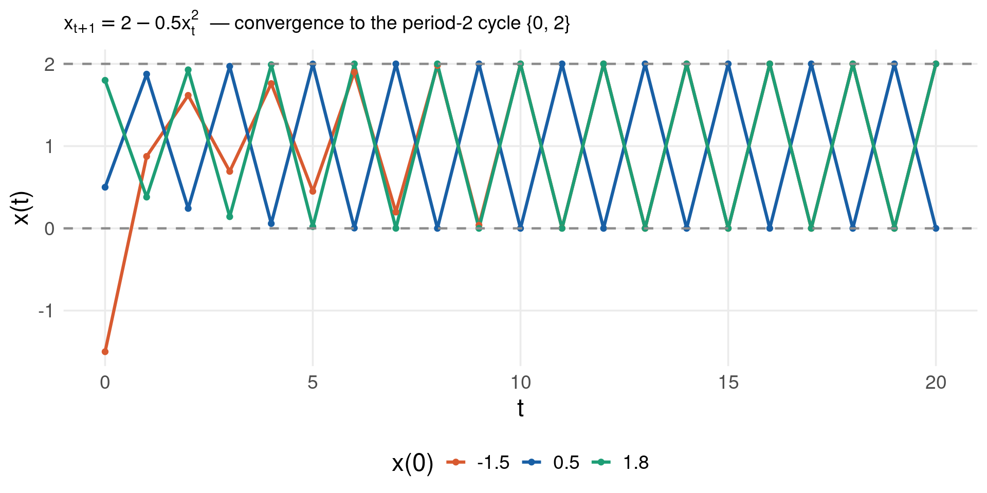
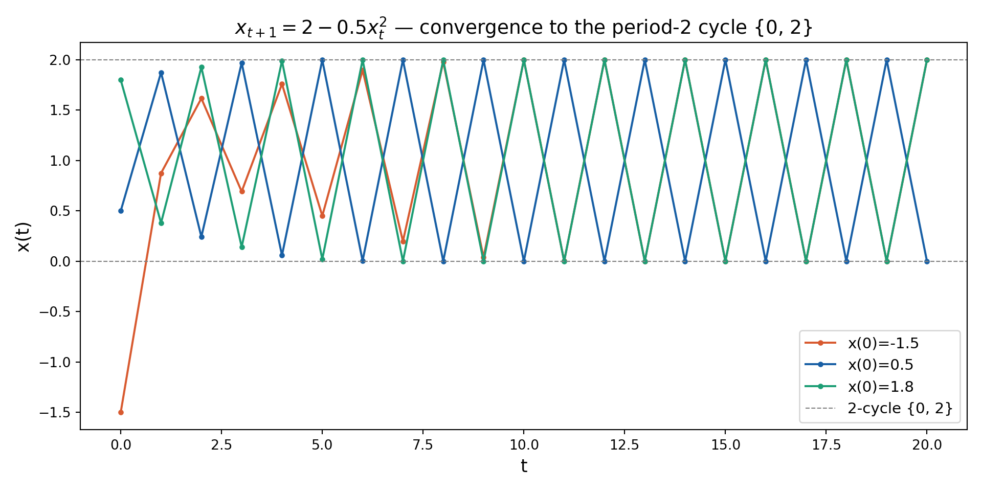
\[x_{t+1} = 2 - 0.5 x_t^2\]

Fixed points: solve \(x^* = 2 - 0.5(x^*)^2\):

\[0.5(x^*)^2 + x^* - 2 = 0 \implies x^* = -1 \pm \sqrt{5}\]

\[x_1^* = -1 + \sqrt{5} \approx 1.236, \qquad x_2^* = -1 - \sqrt{5} \approx -3.236\]

Local stability: \(|f'(x^*)| = |-x^*| = |x^*|\)

  • At \(x_1^* \approx 1.236\): \(|f'| \approx 1.236 > 1\)unstable
  • At \(x_2^* \approx -3.236\): \(|f'| \approx 3.236 > 1\)unstable

Both fixed points repel; trajectories converge instead to the stable period-2 cycle \(\{0, 2\}\), since \(f(0) = 2\) and \(f(2) = 0\) with \(|f'(0)\,f'(2)| = 0 < 1\) (Shone 2001, §1.8).

Nonlinearity & Chaos — The Logistic Map

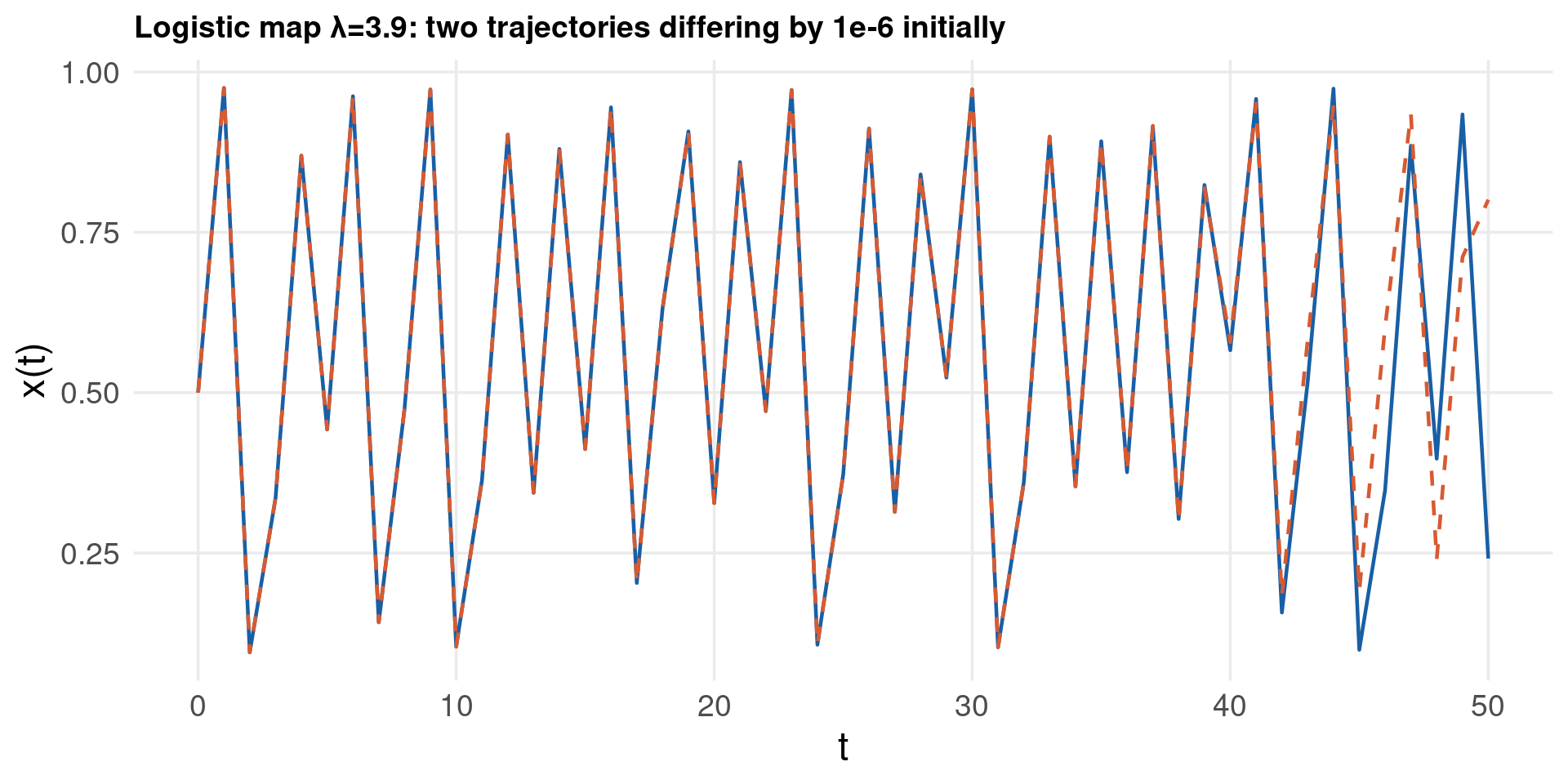
\[x_t = \lambda x_{t-1}(1 - x_{t-1})\]

\(\lambda\) Behaviour
\(0 < \lambda \leq 1\) \(x_t \to 0\)
\(1 < \lambda \leq 3\) converges to \(x^* = 1 - 1/\lambda\)
\(\lambda \approx 3\) period-2 cycle
\(\lambda \approx 3.449\) period-4 cycle
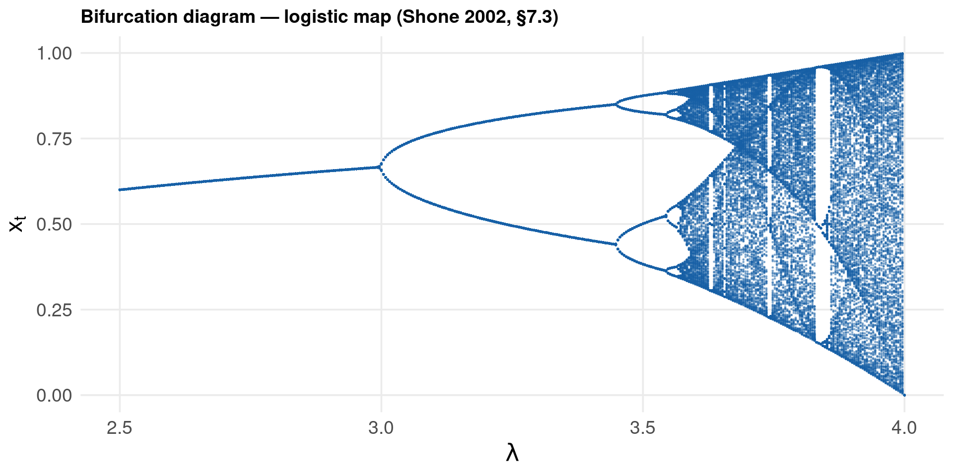
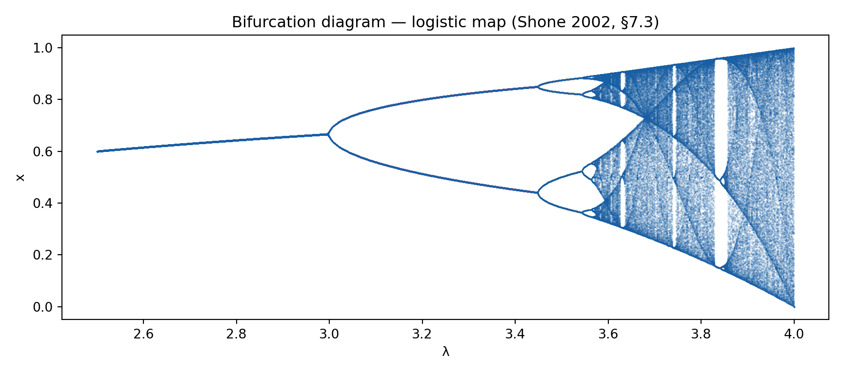
\(\lambda \approx 3.569\) onset of chaos
\(\lambda > 3.57\) chaos

A deterministic equation can produce apparently random behaviour.

\[|f'(x^*)| = |\lambda(1 - 2x^*)| = |2 - \lambda|\]

  • Stable fixed point for \(\lambda \in (1, 3)\): \(|f'| < 1\)
  • Unstable for \(\lambda > 3\): period-doubling begins

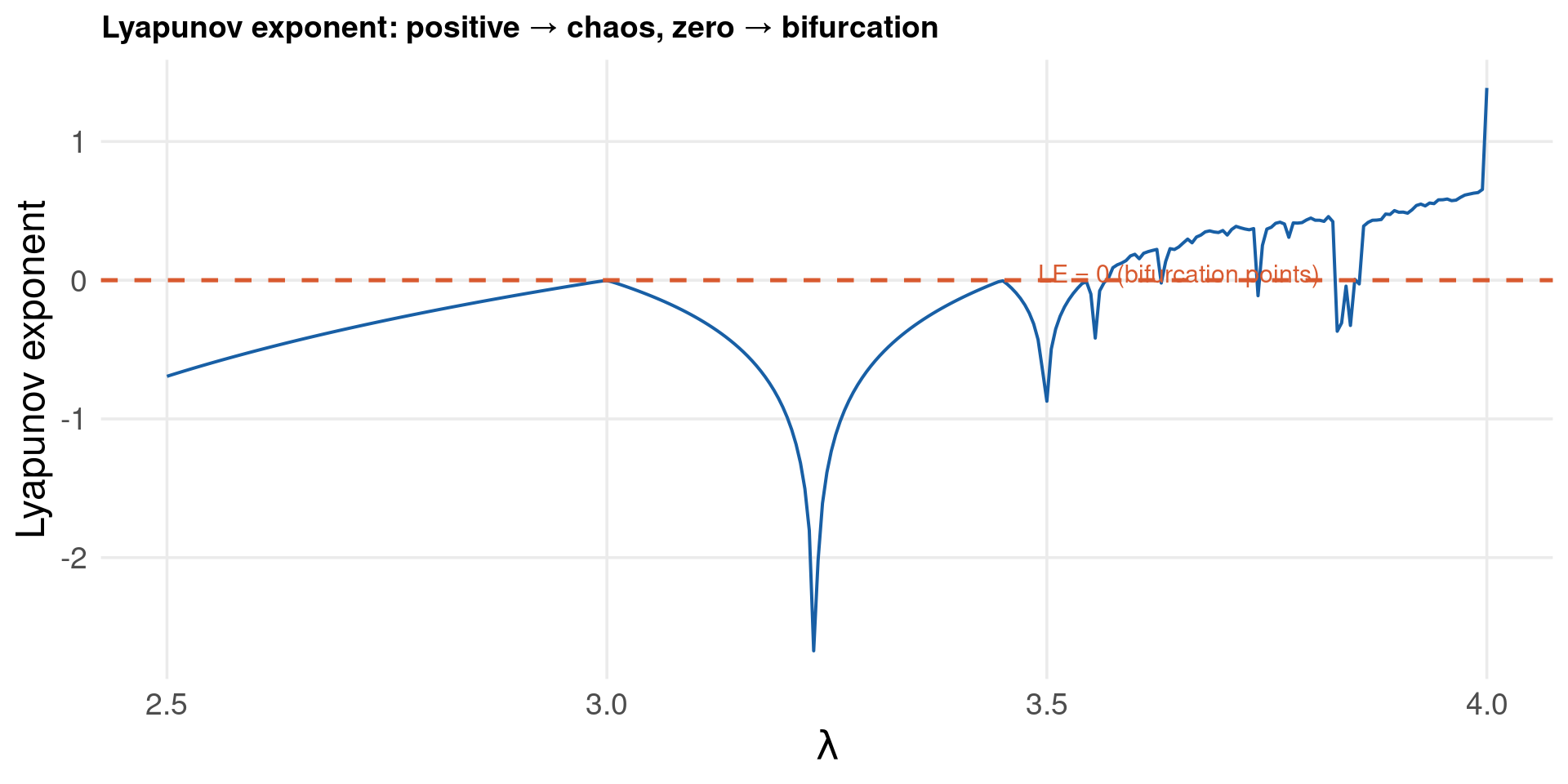
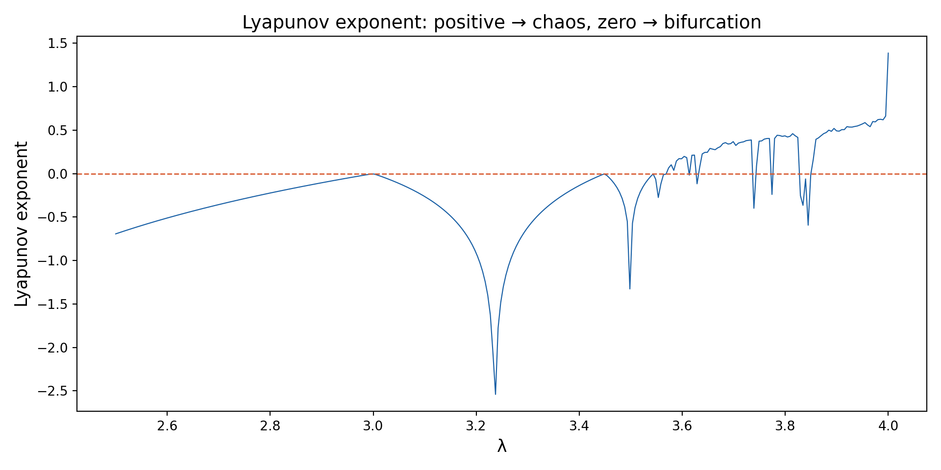
This connects directly to Part VII: Chaos Theory — the full bifurcation diagram shows the complete route from stability to chaos.

First-Order Linear Recursion

First-order linear recursion:

\[x(t+1) = a + b \cdot x(t)\]

Fixed point (set \(x(t+1) = x(t) = x^*\)):

\[x^* = \frac{a}{1-b}, \quad b \neq 1\]

Stability: \(|b| < 1 \Rightarrow x_t \to x^*\)

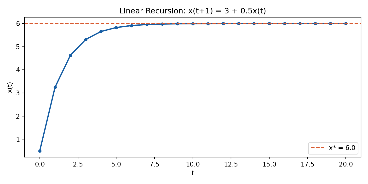
Example: \(x(t+1) = 3 + 0.5 \, x(t)\), so \(x^* = 3/(1-0.5) = 6\)

Code
a <- 3; b <- 0.5
x_star <- a / (1 - b)
T <- 20
x <- numeric(T + 1); x[1] <- 0.5
for (t in seq_len(T)) x[t+1] <- a + b * x[t]

df <- data.frame(t = 0:T, x = x)

ggplot(df) +
  aes(x = t, y = x) +
  geom_line(color = col_main, linewidth = 1) +
  geom_point(color = col_main, size = 2) +
  geom_hline(yintercept = x_star, linetype = "dashed", color = col_accent) +
  annotate("text", x = 15, y = x_star + 0.3,
           label = glue("x* = {x_star}"), color = col_accent, size = 4) +
  labs(x = "t", y = "x(t)", title = "Linear Recursion: x(t+1) = 3 + 0.5x(t)") +
  theme_lecture

Code
import numpy as np
import matplotlib.pyplot as plt

a, b = 3, 0.5
x_star = a / (1 - b)
T = 20
x = np.zeros(T + 1); x[0] = 0.5
for t in range(T):
    x[t+1] = a + b * x[t]

fig, ax = plt.subplots(figsize=(8, 4))
ax.plot(range(T+1), x, color="#185FA5", linewidth=2, marker="o", markersize=4)
ax.axhline(x_star, linestyle="--", color="#D85A30", label=f"x* = {x_star}")
ax.set_xlabel("t"); ax.set_ylabel("x(t)")
ax.set_title("Linear Recursion: x(t+1) = 3 + 0.5x(t)")
ax.legend(); plt.tight_layout(); plt.show()

Nonlinear Recursion Code

Code
f    <- function(x) 2 - 0.5 * x^2
T    <- 20
x    <- numeric(T + 1)

# Three initial conditions
x0s  <- c(-1.5, 0.5, 1.8)
cols <- c(col_accent, col_main, col_ok)

df_list <- lapply(seq_along(x0s), function(i) {
  x[1] <- x0s[i]
  for (t in seq_len(T)) x[t+1] <- f(x[t])
  data.frame(t = 0:T, x = x, x0 = x0s[i])
})

bind_rows(df_list) %>%
  ggplot() +
  aes(x = t, y = x, color = factor(x0)) +
  geom_line(linewidth = 1.1) +
  geom_point(size = 1.5) +
  geom_hline(yintercept = c(0, 2), linetype = "dashed", color = col_muted,
             linewidth = 0.8) +
  scale_color_manual(values = cols, name = "x(0)") +
  labs(x = "t", y = "x(t)", title = expression(x[t+1] == 2 - 0.5*x[t]^2 ~ " — convergence to the period-2 cycle {0, 2}")) +
  theme_lecture

Code
import numpy as np
import matplotlib.pyplot as plt

f = lambda x: 2 - 0.5 * x**2
T = 20
x0s   = [-1.5, 0.5, 1.8]
colors = ["#D85A30", "#185FA5", "#1D9E75"]

fig, ax = plt.subplots(figsize=(10, 5))
for x0, c in zip(x0s, colors):
    x = np.zeros(T + 1); x[0] = x0
    for t in range(T): x[t+1] = f(x[t])
    ax.plot(range(T+1), x, color=c, linewidth=1.5, marker="o",
            markersize=3, label=f"x(0)={x0}")
ax.axhline(0, linestyle="--", color="grey", linewidth=0.8, label="2-cycle {0, 2}")
ax.axhline(2, linestyle="--", color="grey", linewidth=0.8)
ax.set_xlabel("t", fontsize=13); ax.set_ylabel("x(t)", fontsize=13)
ax.set_title(r"$x_{t+1} = 2 - 0.5x_t^2$ — convergence to the period-2 cycle {0, 2}", fontsize=14)
ax.legend(fontsize=11); plt.tight_layout(); plt.show()

Types of Time Paths

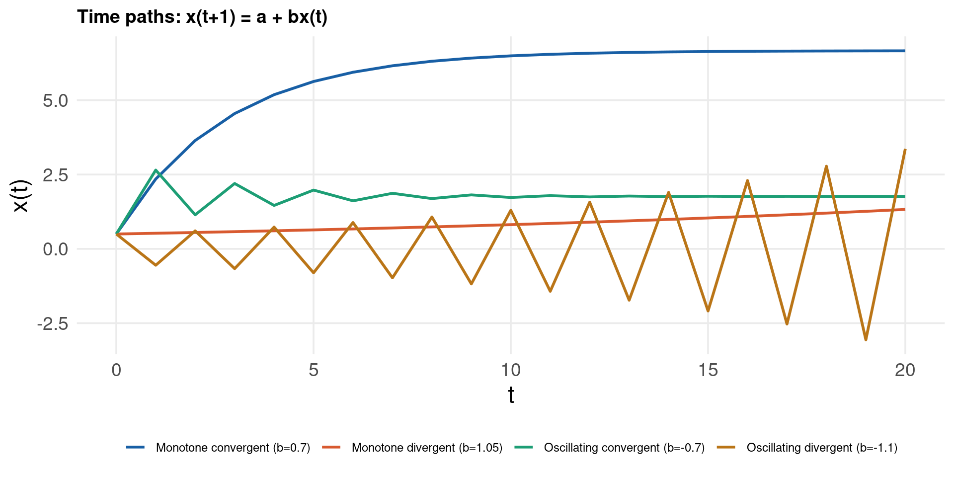
Seven canonical time paths in dynamic models:

Path type Condition Example
Monotone convergent \(0 < b < 1\) savings → steady state
Monotone divergent \(b > 1\) explosive growth
Oscillating convergent \(-1 < b < 0\) converging cobweb
Oscillating divergent \(b < -1\) diverging cobweb
Periodic (period-2) \(b = -1\) perpetual oscillation
Constant \(b = 0\) static
Exponential continuous, \(b>0\) Harrod-Domar
Code
T <- 20
paths <- list(
  list(a=2, b=0.7,  x0=0.5, label="Monotone convergent (b=0.7)"),
  list(a=0, b=1.05, x0=0.5, label="Monotone divergent (b=1.05)"),
  list(a=3, b=-0.7, x0=0.5, label="Oscillating convergent (b=-0.7)"),
  list(a=0, b=-1.1, x0=0.5, label="Oscillating divergent (b=-1.1)")
)
cols_p <- c(col_main, col_accent, col_ok, col_warn)

df_paths <- lapply(seq_along(paths), function(i) {
  p <- paths[[i]]
  x <- numeric(T + 1); x[1] <- p$x0
  for (t in seq_len(T)) x[t+1] <- p$a + p$b * x[t]
  data.frame(t = 0:T, x = x, type = p$label)
})

bind_rows(df_paths) %>%
  ggplot() +
  aes(x = t, y = x, color = type) +
  geom_line(linewidth = 1) +
  scale_color_manual(values = cols_p, name = NULL) +
  labs(x = "t", y = "x(t)", title = "Time paths: x(t+1) = a + bx(t)") +
  theme_lecture + theme(legend.position = "bottom", legend.text = element_text(size = 9))

Part II: Continuous Dynamic Systems

ODEs, phase portraits, and economic growth

First-Order Linear ODEs

Homogeneous: \(\dot{x} = ax\)

\[x(t) = x(0) \, e^{at}, \quad a < 0 \text{ → stable}, \quad a > 0 \text{ → explosive}\]

Non-homogeneous: \(\dot{x} = a + bx\)

Equilibrium: \(x^* = -a/b\)

\[x(t) = x^* + [x(0) - x^*] e^{bt}, \quad \text{stable if } b < 0\]

Harrod-Domar growth:

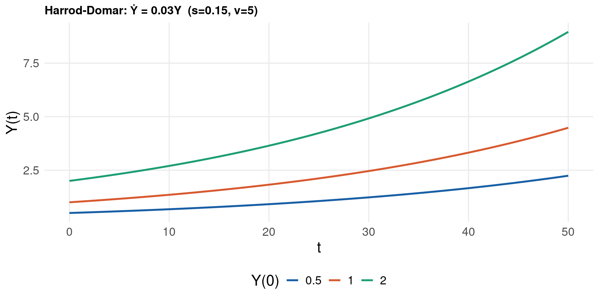
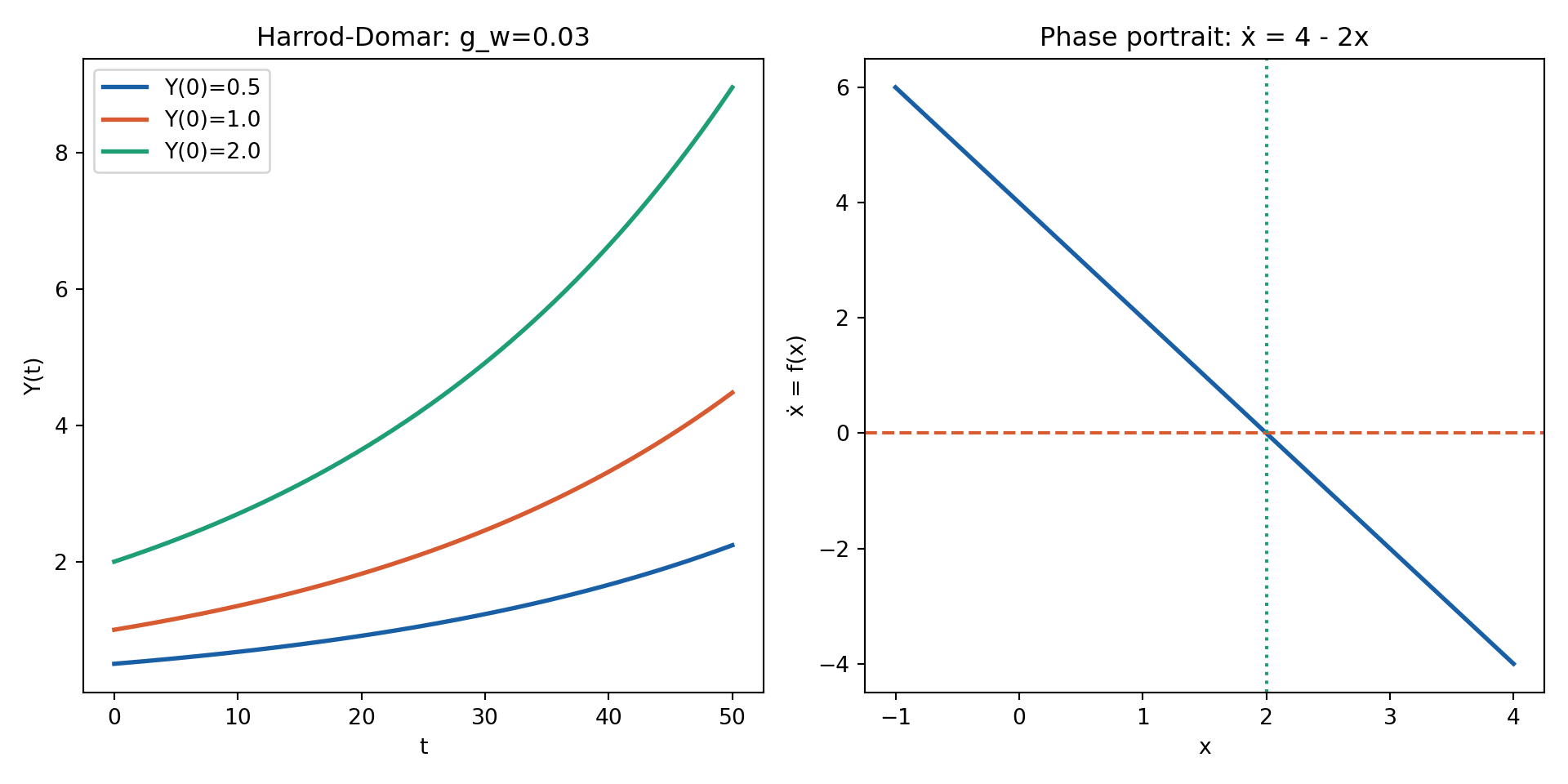
\[\dot{Y} = \frac{s}{v} Y \implies Y(t) = Y(0) \, e^{(s/v)t}, \quad g_w = s/v\]

Growth is explosive — no convergence without diminishing returns.

Phase portrait: plot \(\dot{x} = f(x)\) vs. \(x\); stable equilibrium where \(f'(x^*) < 0\).

Code
rhs <- function(t, y, parms) list(parms$a + parms$b * y[1])
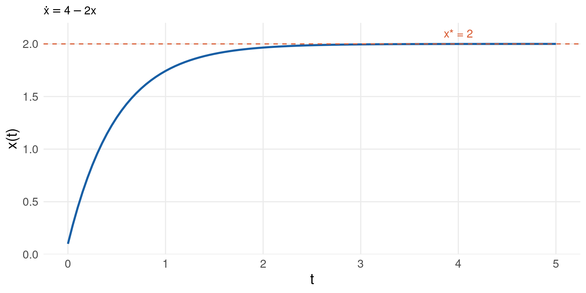
parms <- list(a = 4, b = -2)   # ẋ = 4 - 2x → x* = 2
sol   <- ode(y = c(x = 0.1), times = seq(0, 5, by = 0.05),
             func = rhs, parms = parms)

as.data.frame(sol) %>%
  ggplot() +
  aes(x = time, y = x) +
  geom_line(color = col_main, linewidth = 1.4) +
  geom_hline(yintercept = 2, linetype = "dashed", color = col_accent, linewidth = 1) +
  annotate("text", x = 4, y = 2.15, label = "x* = 2", color = col_accent, size = 5) +
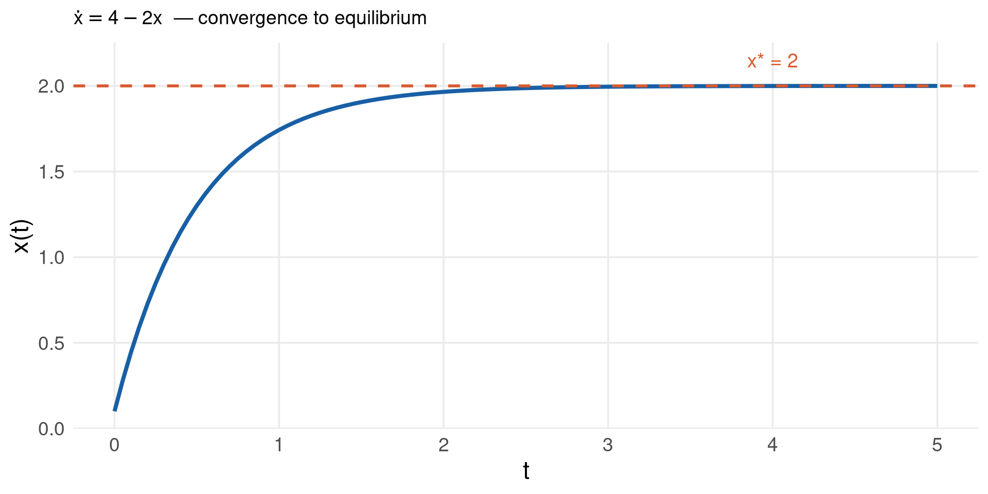
  labs(x = "t", y = "x(t)", title = expression(dot(x) == 4 - 2*x ~ " — convergence to equilibrium")) +
  theme_lecture

Code
import numpy as np
import matplotlib.pyplot as plt
from scipy.integrate import solve_ivp

sol = solve_ivp(lambda t, y: [4 - 2*y[0]], [0, 5], [0.1],
                t_eval=np.linspace(0, 5, 200))

fig, ax = plt.subplots(figsize=(10, 5))
ax.plot(sol.t, sol.y[0], color="#185FA5", linewidth=2, label="x(t)")
ax.axhline(2, linestyle="--", color="#D85A30", linewidth=1.5, label="x* = 2")
ax.set_xlabel("t", fontsize=13); ax.set_ylabel("x(t)", fontsize=13)
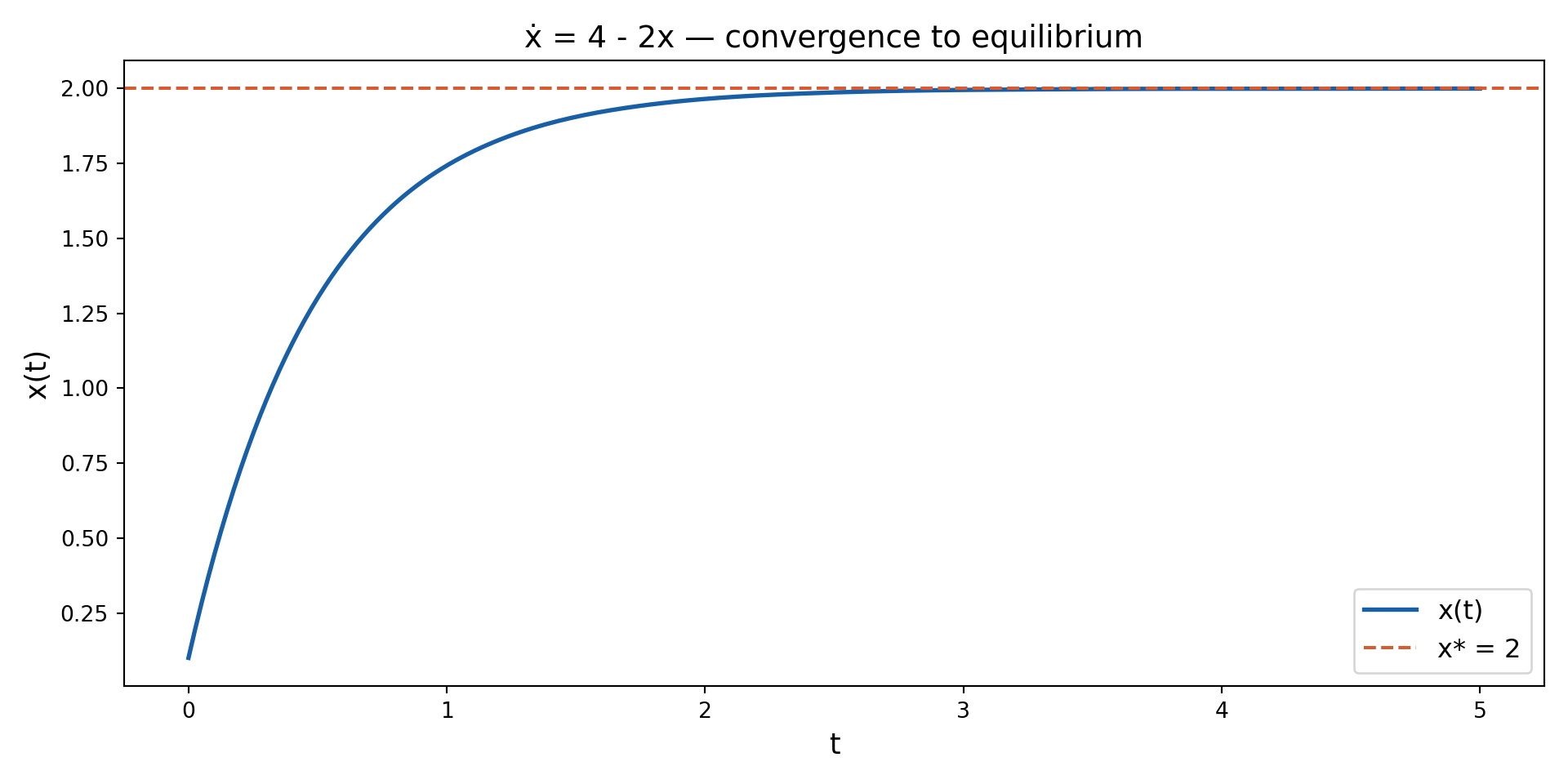
ax.set_title("ẋ = 4 - 2x — convergence to equilibrium", fontsize=14)
ax.legend(fontsize=12); plt.tight_layout(); plt.show()

Solving First-Order ODEs: Integrating Factor

General form: \(\dot{x} = a + bx\), rewrite as

\[\dot{x} - bx = a\]

Step 1 — integrating factor: multiply both sides by \(\mu(t) = e^{-bt}\)

\[e^{-bt}\dot{x} - b\,e^{-bt}x = a\,e^{-bt}\]

Step 2 — recognise the left-hand side as an exact derivative

\[\frac{d}{dt}\!\left[x\,e^{-bt}\right] = a\,e^{-bt}\]

Step 3 — integrate both sides

\[x(t)\,e^{-bt} = -\frac{a}{b}\,e^{-bt} + C\]

Step 4 — solve for \(x(t)\) (multiply through by \(e^{bt}\))

\[x(t) = -\frac{a}{b} + C\,e^{bt} = x^* + C\,e^{bt}, \qquad x^* = -\frac{a}{b}\]

Step 5 — apply initial condition \(x(0) = x_0\)

\[x_0 = x^* + C \implies C = x_0 - x^*\]

\[\boxed{x(t) = x^* + (x_0 - x^*)\,e^{bt}}\]

Code
a_s <- 4; b_s <- -2          # ẋ = 4 - 2x  →  x* = 2
x0_s <- 0.1
x_star_s <- -a_s / b_s       # analytical equilibrium

t_grid <- seq(0, 5, by = 0.05)

# Closed-form solution (Step 5 formula)
x_exact <- x_star_s + (x0_s - x_star_s) * exp(b_s * t_grid)

# Numerical solution via deSolve
rhs_s <- function(t, y, parms) list(parms$a + parms$b * y[1])
sol_s  <- ode(y = c(x = x0_s), times = t_grid,
              func = rhs_s, parms = list(a = a_s, b = b_s))

df_compare <- data.frame(
  t       = t_grid,
  exact   = x_exact,
  numeric = as.data.frame(sol_s)$x
)

df_compare %>%
  ggplot() +
  aes(x = t) +
  geom_line(aes(y = exact),   color = col_main,   linewidth = 1.8, linetype = "solid") +
  geom_line(aes(y = numeric), color = col_accent,  linewidth = 0.8, linetype = "dashed") +
  geom_hline(yintercept = x_star_s, linetype = "dotted", color = col_muted) +
  annotate("text", x = 4, y = x_star_s + 0.12,
           label = paste0("x* = ", x_star_s), color = col_muted, size = 5) +
  labs(x = "t", y = "x(t)",
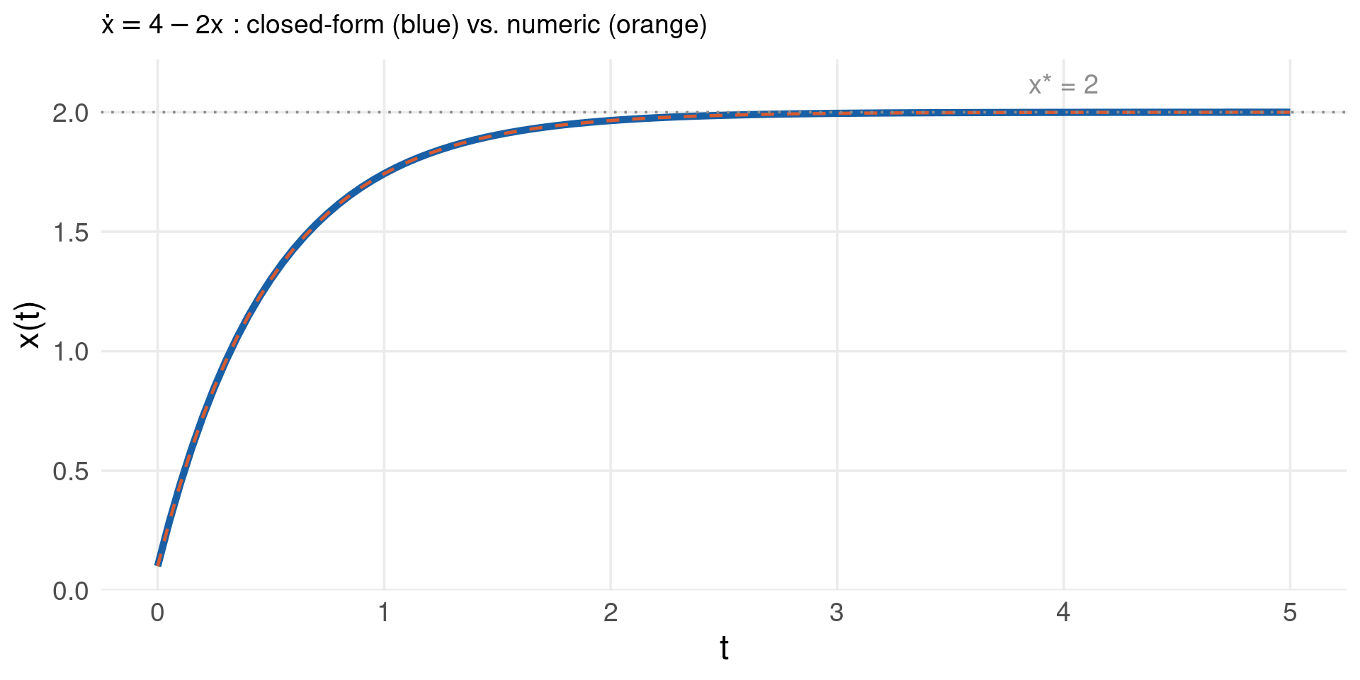
       title = expression(dot(x) == 4 - 2*x ~ ": closed-form (blue) vs. numeric (orange)")) +
  theme_lecture

Code
import sympy as sp
import numpy as np
import matplotlib.pyplot as plt
from scipy.integrate import solve_ivp

# --- Symbolic solution via sympy ---
t, C1 = sp.symbols("t C1")
x = sp.Function("x")

ode_eq = sp.Eq(x(t).diff(t), 4 - 2*x(t))
sol_sym = sp.dsolve(ode_eq, x(t))
print("General solution:")
General solution:
Code
sp.pprint(sol_sym)
           -2*t    
x(t) = C1*e     + 2
Code
# Apply initial condition x(0) = 0.1
C_val = sp.solve(sol_sym.rhs.subs(t, 0) - 0.1, C1)[0]
sol_particular = sol_sym.rhs.subs(C1, C_val)
print(f"\nParticular solution (x0=0.1):  x(t) = {sol_particular}")

Particular solution (x0=0.1):  x(t) = 2 - 1.9*exp(-2*t)
Code
# --- Numerical solution via scipy ---
t_eval = np.linspace(0, 5, 300)
num = solve_ivp(lambda t, y: [4 - 2*y[0]], [0, 5], [0.1], t_eval=t_eval)

# Evaluate closed form
x_exact = float(C_val) * np.exp(-2 * t_eval) + 2.0

fig, ax = plt.subplots(figsize=(10, 5))
ax.plot(t_eval, x_exact,      color="#185FA5", linewidth=2.0, label="Closed form (sympy)")
ax.plot(num.t,  num.y[0],     color="#D85A30", linewidth=0.9,
        linestyle="dashed",   label="Numeric (scipy)")
ax.axhline(2, linestyle="dotted", color="grey", linewidth=1)
ax.text(4, 2.1, "x* = 2", color="grey", fontsize=12)
ax.set_xlabel("t", fontsize=13)
ax.set_ylabel("x(t)", fontsize=13)
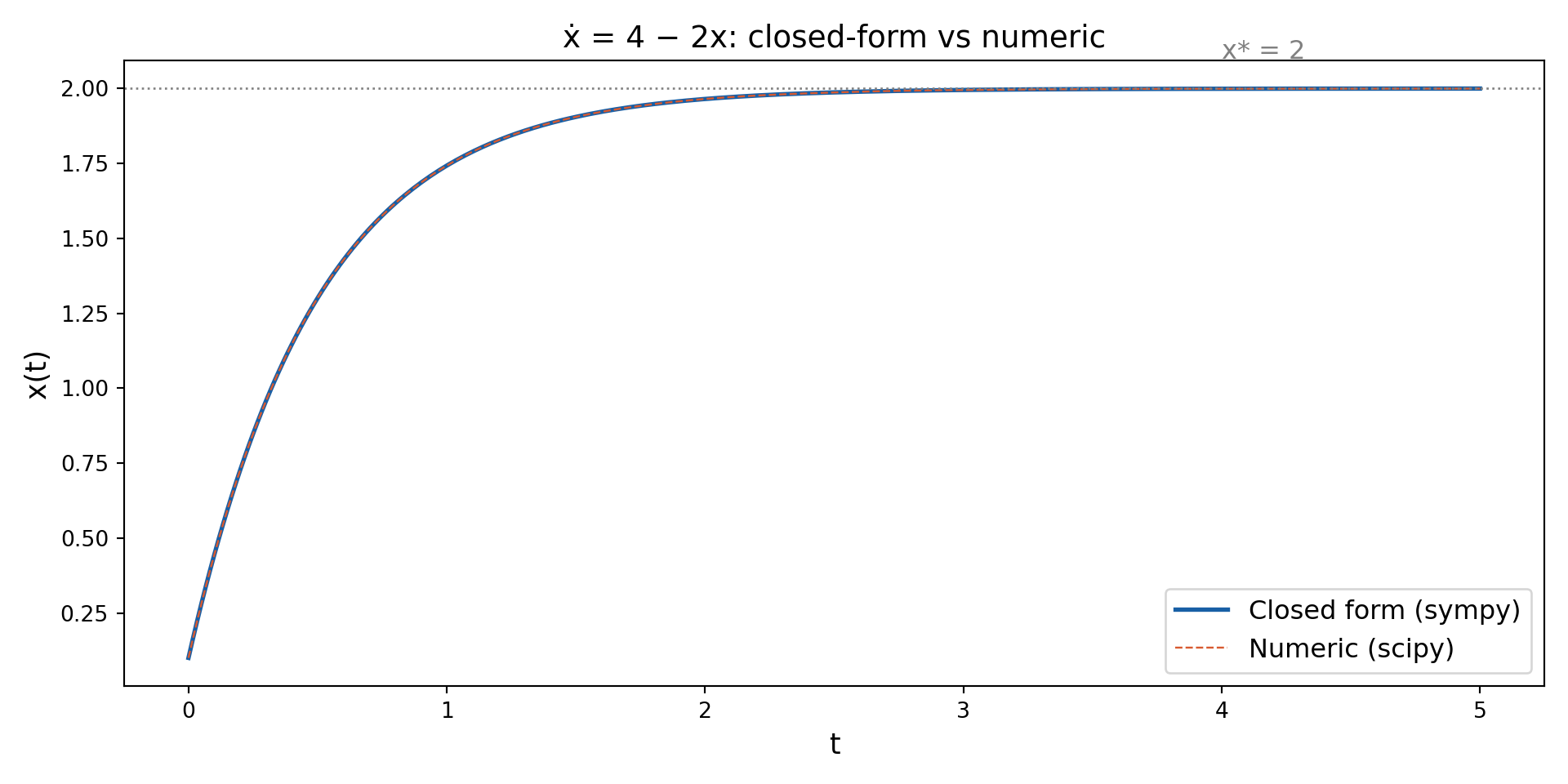
ax.set_title("ẋ = 4 − 2x: closed-form vs numeric", fontsize=14)
ax.legend(fontsize=12)
plt.tight_layout()
plt.show()

Compound Interest & Logistic Growth

Continuous compounding

\[A(t) = A(0) \, e^{rt}\]

Discrete compounding (\(m\) times/year)

\[A_n = A(0)\!\left(1 + \frac{r}{m}\right)^{\!mn} \xrightarrow{m\to\infty} A(0)e^{rt}\]

Separable ODE:

\[\dot{x} = \alpha x \!\left(1 - \frac{x}{K}\right)\]

  • \(K\) = carrying capacity
  • \(x^* = 0\) (unstable), \(x^* = K\) (stable)

Analytical solution (S-curve):

\[x(t) = \frac{K}{1 + \!\left(\dfrac{K - x_0}{x_0}\right)\!e^{-\alpha t}}\]

Economic applications: population growth models, diffusion of new technology, market saturation — any bounded growth process.

Technology/information diffusion (S-curve)

Let \(N\) = total population, \(x(t)\) = adopters:

\[\dot{x} = \beta x(N - x)\]

This is the logistic equation with \(K = N\), \(\alpha = \beta N\).

Solution: \(x(t) = \dfrac{N}{1 + e^{-\beta N(t - t_0)}}\) where \(t_0\) is the inflection point.

Second-Order Linear Homogeneous ODEs

General form:

\[\ddot{x} + a\dot{x} + bx = 0, \qquad x(0) = x_0,\quad \dot{x}(0) = v_0\]

Step 1 — trial solution: assume \(x(t) = e^{rt}\) for some constant \(r\).

Substituting: \(r^2 e^{rt} + a r e^{rt} + b e^{rt} = 0\). Since \(e^{rt} \neq 0\), divide through:

\[r^2 + ar + b = 0 \qquad \text{(characteristic equation)}\]

Step 2 — solve the characteristic equation:

\[r_{1,2} = \frac{-a \pm \sqrt{\Delta}}{2}, \qquad \Delta = a^2 - 4b\]

Step 3 — write general solution according to the sign of \(\Delta\):

\(\Delta\) Roots General solution \(x(t)\) Behaviour
\(> 0\) real distinct \(r_1 \neq r_2\) \(A e^{r_1 t} + B e^{r_2 t}\) monotone
\(= 0\) repeated \(r_1 = r_2 = r\) \((A + Bt)e^{rt}\) monotone with \(t\)-weight
\(< 0\) complex \(\alpha \pm \beta i\) \(e^{\alpha t}(A\cos\beta t + B\sin\beta t)\) oscillatory

Step 4 — apply initial conditions to pin down \(A\) and \(B\) (shown in each case tab).

\[r_1 = \frac{-a + \sqrt{\Delta}}{2}, \quad r_2 = \frac{-a - \sqrt{\Delta}}{2}, \quad r_1 \neq r_2\]

General solution:

\[x(t) = A e^{r_1 t} + B e^{r_2 t}\]

Apply initial conditions \(x(0) = x_0\), \(\dot{x}(0) = v_0\):

\[A + B = x_0, \qquad r_1 A + r_2 B = v_0\]

Solving the \(2 \times 2\) system:

\[A = \frac{v_0 - r_2\, x_0}{r_1 - r_2}, \qquad B = \frac{r_1\, x_0 - v_0}{r_1 - r_2}\]

Stability: both roots must be negative \(\Rightarrow\) \(r_1 < 0\) and \(r_2 < 0\), which requires \(a > 0\) and \(b > 0\).

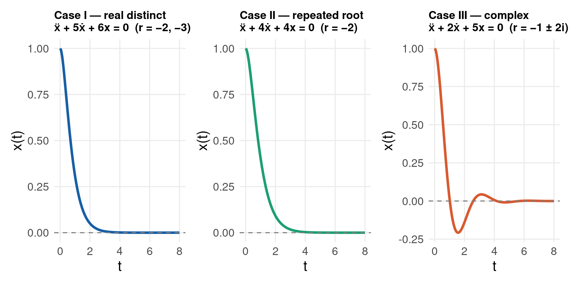
Example: \(\ddot{x} + 5\dot{x} + 6x = 0\) \(\;\Rightarrow\;\) \(r^2 + 5r + 6 = (r+2)(r+3) = 0\) \(\;\Rightarrow\;\) \(r_1 = -2,\; r_2 = -3\).

With \(x_0 = 1\), \(v_0 = 0\): \(A = (0 - (-3)\cdot 1)/(-2-(-3)) = 3\), \(B = (-2\cdot 1 - 0)/(-2-(-3)) = -2\).

\[x(t) = 3e^{-2t} - 2e^{-3t} \xrightarrow{t\to\infty} 0 \quad \checkmark\]

\[r = -\frac{a}{2} \qquad (\text{double root})\]

When \(\Delta = 0\) the two basis functions \(e^{r_1 t}\) and \(e^{r_2 t}\) coincide, so we need a second independent solution. It can be shown by reduction of order that \(t e^{rt}\) is the missing solution.

General solution:

\[x(t) = (A + Bt)\,e^{rt}\]

Apply initial conditions \(x(0) = x_0\), \(\dot{x}(0) = v_0\):

\[\dot{x}(t) = B e^{rt} + (A + Bt) r e^{rt}\]

At \(t = 0\): \(A = x_0\) and \(B + r A = v_0\), so \(B = v_0 - r x_0\).

Stability: \(r < 0 \Leftrightarrow a > 0\) (and \(b = a^2/4 > 0\) automatically).

Example: \(\ddot{x} + 4\dot{x} + 4x = 0\) \(\;\Rightarrow\;\) \(r = -2\).

With \(x_0 = 1\), \(v_0 = 0\): \(A = 1\), \(B = 0 - (-2)(1) = 2\).

\[x(t) = (1 + 2t)\,e^{-2t}\]

\[r_{1,2} = \alpha \pm \beta i, \qquad \alpha = -\frac{a}{2}, \quad \beta = \frac{\sqrt{4b - a^2}}{2}\]

Using Euler’s formula \(e^{i\theta} = \cos\theta + i\sin\theta\), the two complex exponentials combine into:

\[x(t) = e^{\alpha t}(A\cos\beta t + B\sin\beta t)\]

  • \(e^{\alpha t}\): envelope — grows if \(\alpha > 0\), decays if \(\alpha < 0\)
  • \(\cos\beta t,\; \sin\beta t\): oscillation with period \(T = 2\pi/\beta\), frequency \(f = \beta/(2\pi)\)

Apply initial conditions \(x(0) = x_0\), \(\dot{x}(0) = v_0\):

\[A = x_0, \qquad B = \frac{v_0 - \alpha x_0}{\beta}\]

Stability: \(\alpha < 0 \Leftrightarrow a > 0\) (with \(b > 0\) ensuring \(\beta \in \mathbb{R}\)).

Example: \(\ddot{x} + 2\dot{x} + 5x = 0\) \(\;\Rightarrow\;\) \(\alpha = -1\), \(\beta = 2\).

With \(x_0 = 1\), \(v_0 = 0\): \(A = 1\), \(B = (0 - (-1)(1))/2 = 0.5\).

\[x(t) = e^{-t}(\cos 2t + 0.5\sin 2t) \quad \text{— damped oscillation}\]

Routh–Hurwitz conditions for \(r^2 + ar + b = 0\):

\[\boxed{a > 0 \quad \text{and} \quad b > 0} \quad \Longrightarrow \quad \text{Re}(r_{1,2}) < 0 \quad \Longrightarrow \quad x(t) \to 0\]

The conditions are necessary and sufficient — check them without computing the roots.

\(a\) \(b\) Verdict
\(> 0\) \(> 0\) stable — all roots have negative real part
\(> 0\) \(< 0\) unstable — one root positive
\(< 0\) any unstable — roots sum to \(-a > 0\)
\(= 0\) \(> 0\) centre — pure oscillation, \(\text{Re}(r) = 0\)

Economic interpretation: for a second-order economic model (e.g. multiplier-accelerator, inventory cycle), stability requires both a positive damping coefficient (\(a > 0\), friction in adjustment) and a positive restoring force (\(b > 0\), tendency to return to equilibrium).

Second-Order ODE — Code (Three Cases)

Code
library(patchwork)

# Convert ẍ + aẋ + bx = 0  to system: y1=x, y2=ẋ
ode2_rhs <- function(t, y, parms) {
  list(c(y[2], -parms$b * y[1] - parms$a * y[2]))
}
solve2 <- function(a, b, x0 = 1, v0 = 0, tmax = 8) {
  ode(y = c(x = x0, v = v0), times = seq(0, tmax, by = 0.05),
      func = ode2_rhs, parms = list(a = a, b = b)) %>%
    as.data.frame()
}

# Three cases
df1 <- solve2(a = 5, b = 6)         # Case I:  r = -2, -3  (real distinct)
df2 <- solve2(a = 4, b = 4)         # Case II: r = -2, -2  (repeated)
df3 <- solve2(a = 2, b = 5)         # Case III: r = -1±2i  (complex, damped)

make_plot <- function(df, title, col) {
  df %>%
    ggplot() +
    aes(x = time, y = x) +
    geom_line(color = col, linewidth = 1.5) +
    geom_hline(yintercept = 0, linetype = "dashed", color = "grey50") +
    labs(x = "t", y = "x(t)", title = title) +
    theme_lecture
}

p1 <- make_plot(df1, "Case I — real distinct\nẍ + 5ẋ + 6x = 0  (r = −2, −3)", col_main)
p2 <- make_plot(df2, "Case II — repeated root\nẍ + 4ẋ + 4x = 0  (r = −2)",     col_ok)
p3 <- make_plot(df3, "Case III — complex\nẍ + 2ẋ + 5x = 0  (r = −1 ± 2i)",    col_accent)

p1 + p2 + p3

Code
import sympy as sp
import numpy as np
import matplotlib.pyplot as plt
from scipy.integrate import solve_ivp

t = sp.Symbol("t")
x = sp.Function("x")

def solve_ode2_sym(a, b, x0=1, v0=0, label=""):
    ode_eq = sp.Eq(x(t).diff(t, 2) + a*x(t).diff(t) + b*x(t), 0)
    sol = sp.dsolve(ode_eq, x(t),
                    ics={x(0): x0, x(t).diff(t).subs(t, 0): v0})
    print(f"\n{'─'*55}")
    print(f"  {label}:  ẍ + {a}ẋ + {b}x = 0")
    sp.pprint(sol)
    return sp.lambdify(t, sol.rhs, "numpy")

cases = [
    (5, 6, "Case I  — real distinct  r = −2, −3"),
    (4, 4, "Case II — repeated root  r = −2"),
    (2, 5, "Case III — complex       r = −1 ± 2i"),
]
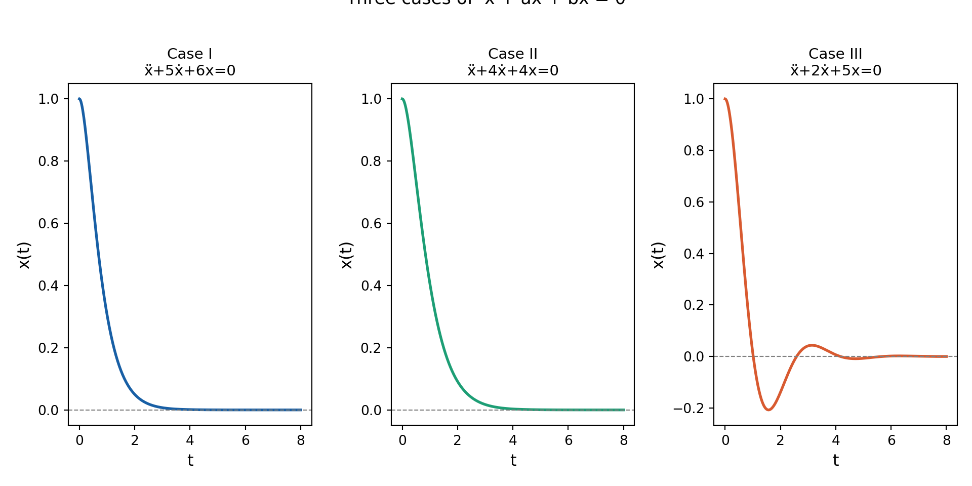
fns = [solve_ode2_sym(a, b, label=lbl) for a, b, lbl in cases]

───────────────────────────────────────────────────────
  Case I  — real distinct  r = −2, −3:  ẍ + 5ẋ + 6x = 0
       /       -t\  -2*t
x(t) = \3 - 2*e  /*e    

───────────────────────────────────────────────────────
  Case II — repeated root  r = −2:  ẍ + 4ẋ + 4x = 0
                  -2*t
x(t) = (2*t + 1)*e    

───────────────────────────────────────────────────────
  Case III — complex       r = −1 ± 2i:  ẍ + 2ẋ + 5x = 0
       /sin(2*t)           \  -t
x(t) = |-------- + cos(2*t)|*e  
       \   2               /    
Code
# Plot all three
t_eval = np.linspace(0, 8, 400)
colors = ["#185FA5", "#1D9E75", "#D85A30"]
labels = ["Case I\nẍ+5ẋ+6x=0", "Case II\nẍ+4ẋ+4x=0", "Case III\nẍ+2ẋ+5x=0"]

fig, axes = plt.subplots(1, 3, figsize=(10, 5), sharey=False)
for ax, fn, col, lbl in zip(axes, fns, colors, labels):
    ax.plot(t_eval, fn(t_eval), color=col, linewidth=2)
    ax.axhline(0, color="grey", linewidth=0.8, linestyle="--")
    ax.set_xlabel("t", fontsize=12)
    ax.set_ylabel("x(t)", fontsize=12)
    ax.set_title(lbl, fontsize=11)
plt.suptitle("Three cases of  ẍ + aẋ + bx = 0", fontsize=13, y=1.02)
plt.tight_layout()
plt.show()

Linearisation near fixed point \(x^*\) — reduction to first order:

For \(\dot{x} = f(x)\) near \(x^*\), let \(z = x - x^*\):

\[\dot{z} \approx f'(x^*)\cdot z \quad \Rightarrow \quad z(t) = z_0\,e^{f'(x^*)t}\]

Stability: \(f'(x^*) < 0\). This converts any smooth nonlinear ODE into a first-order linear system near equilibrium.

Euler approximation — discretise the derivative:

\[x(t + h) \approx x(t) + h\,f\!\bigl(x(t)\bigr)\]

For a second-order system keep both \(x\) and \(\dot{x}\):

\[\begin{bmatrix}x_{n+1}\\\dot{x}_{n+1}\end{bmatrix} \approx \begin{bmatrix}x_n + h\,\dot{x}_n\\\dot{x}_n + h\,\ddot{x}_n\end{bmatrix}, \qquad \ddot{x}_n = -a\,\dot{x}_n - b\,x_n\]

The Euler Method — How It Works

Goal: approximate the solution of \(\dot{x} = f(t, x)\), \(x(t_0) = x_0\) without an analytic formula.

Step 1 — Taylor expansion of \(x(t)\) around \(t_n\):

\[x(t_n + h) = x(t_n) + h\,\dot{x}(t_n) + \frac{h^2}{2}\ddot{x}(t_n) + \mathcal{O}(h^3)\]

Step 2 — truncate after the linear term (drop \(\mathcal{O}(h^2)\) and higher):

\[x(t_n + h) \approx x(t_n) + h\,\dot{x}(t_n)\]

Step 3 — substitute the ODE \(\dot{x}(t_n) = f(t_n, x(t_n))\):

\[\boxed{x_{n+1} = x_n + h\,f(t_n, x_n)}\]

This is the forward Euler update: at each step, walk along the tangent line to the true solution for a distance \(h\).

Step 4 — iterate from \(n = 0\) to build the full trajectory:

\[x_0 \to x_1 \to x_2 \to \cdots \to x_N, \qquad t_n = t_0 + nh\]

Local truncation error (error introduced in one step, assuming the previous point was exact):

\[e_{\text{local}} = x(t_{n+1}) - x_{n+1} = \frac{h^2}{2}\ddot{x}(\xi) = \mathcal{O}(h^2)\]

Global error (accumulated error after \(N = (T-t_0)/h\) steps):

\[e_{\text{global}} = \mathcal{O}(N \cdot h^2) = \mathcal{O}(h)\]

\[\boxed{\text{Euler is a first-order method: halving } h \text{ halves the global error.}}\]

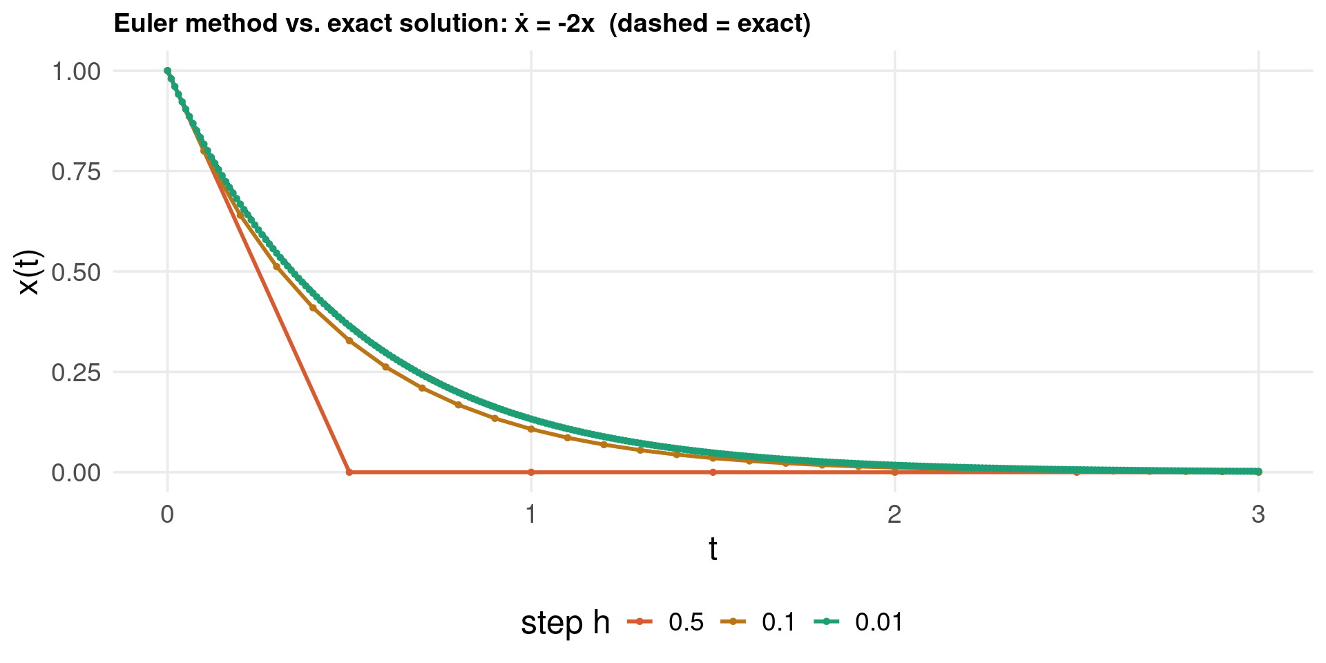
Numerical example: \(\dot{x} = -2x\), \(x_0 = 1\). Exact solution \(x(t) = e^{-2t}\).

Step size \(h\) Euler \(x(1)\) Exact \(x(1)\) Absolute error
\(0.5\) \(0.000\) \(0.1353\) \(0.1353\)
\(0.1\) \(0.1216\) \(0.1353\) \(0.0137\)
\(0.01\) \(0.1340\) \(0.1353\) \(0.0013\)
\(0.001\) \(0.1352\) \(0.1353\) \(0.0001\)

Each ten-fold reduction in \(h\) reduces the error by roughly ten-fold — confirming \(\mathcal{O}(h)\) global convergence.

Code
# Hand-written Euler integrator: dx/dt = f(t, x)
euler_step <- function(f, x, t, h) x + h * f(t, x)

euler_solve <- function(f, x0, t0, tmax, h) {
  n_steps <- floor((tmax - t0) / h)
  t_vec <- t0 + (0:n_steps) * h
  x_vec <- numeric(n_steps + 1); x_vec[1] <- x0
  for (n in seq_len(n_steps)) {
    x_vec[n + 1] <- euler_step(f, x_vec[n], t_vec[n], h)
  }
  data.frame(t = t_vec, x = x_vec)
}

f_decay <- function(t, x) -2 * x     # ẋ = -2x
exact   <- function(t) exp(-2 * t)

# Compare several step sizes against the exact solution
step_sizes <- c(0.5, 0.1, 0.01)
euler_runs <- lapply(step_sizes, function(h) {
  euler_solve(f_decay, x0 = 1, t0 = 0, tmax = 3, h = h) %>%
    mutate(h = factor(h))
})

t_fine <- seq(0, 3, by = 0.01)
df_exact <- data.frame(t = t_fine, x = exact(t_fine))

bind_rows(euler_runs) %>%
  ggplot() +
  aes(x = t, y = x, color = h) +
  geom_line(data = df_exact, aes(x = t, y = x),
            inherit.aes = FALSE, color = "black", linewidth = 1, linetype = "dashed") +
  geom_line(linewidth = 1) +
  geom_point(size = 1) +
  scale_color_manual(values = c(col_accent, col_warn, col_ok), name = "step h") +
  labs(x = "t", y = "x(t)",
       title = "Euler method vs. exact solution: ẋ = -2x  (dashed = exact)") +
  theme_lecture

Code
import numpy as np
import matplotlib.pyplot as plt

def euler_step(f, x, t, h):
    return x + h * f(t, x)

def euler_solve(f, x0, t0, tmax, h):
    n_steps = int(np.floor((tmax - t0) / h))
    t_vec = t0 + np.arange(n_steps + 1) * h
    x_vec = np.zeros(n_steps + 1)
    x_vec[0] = x0
    for n in range(n_steps):
        x_vec[n + 1] = euler_step(f, x_vec[n], t_vec[n], h)
    return t_vec, x_vec

f_decay = lambda t, x: -2 * x
exact   = lambda t: np.exp(-2 * t)

step_sizes = [0.5, 0.1, 0.01]
colors     = ["#D85A30", "#BA7517", "#1D9E75"]

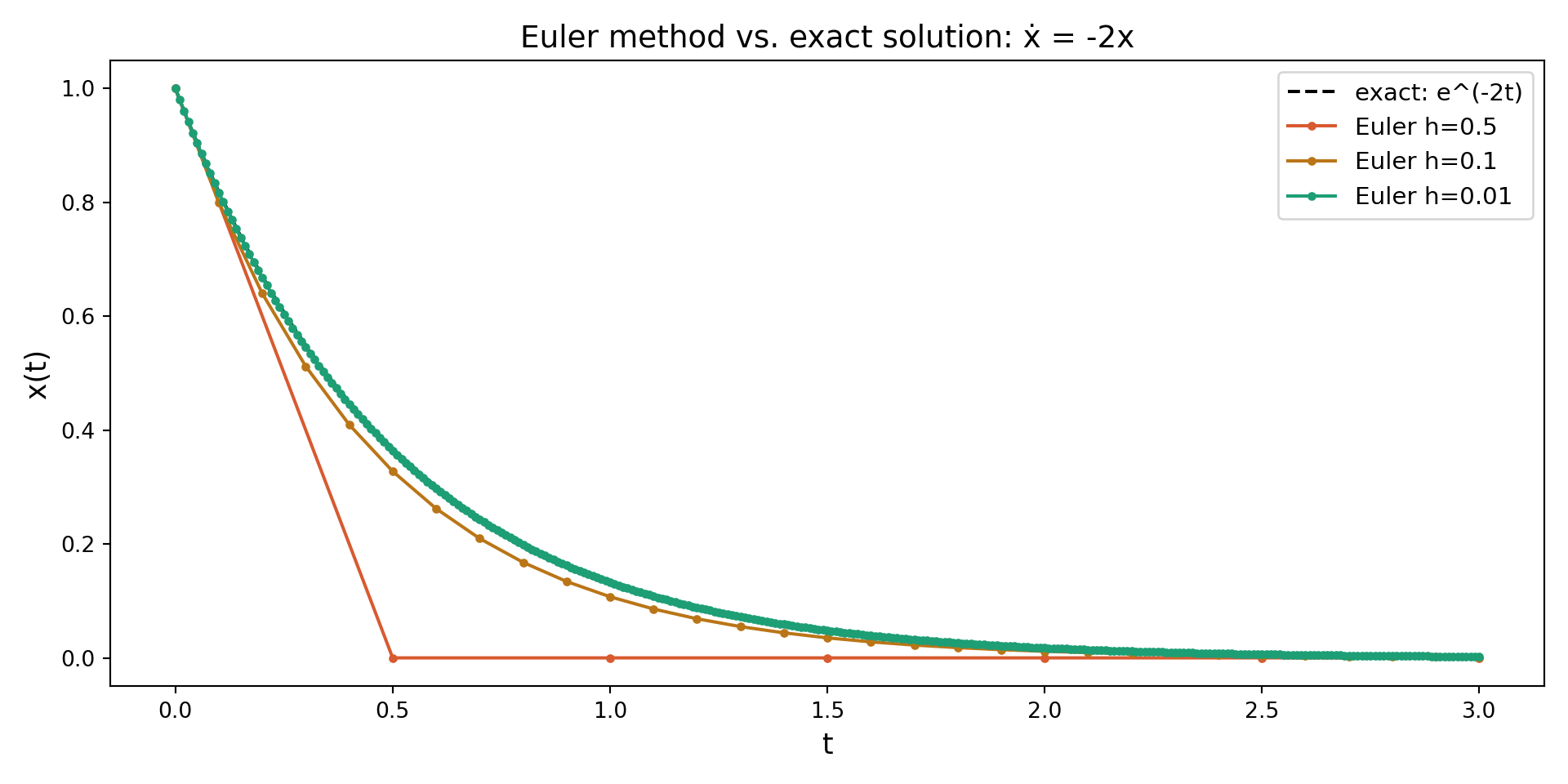
t_fine = np.linspace(0, 3, 300)

fig, ax = plt.subplots(figsize=(10, 5))
ax.plot(t_fine, exact(t_fine), color="black", linewidth=1.5,
        linestyle="dashed", label="exact: e^(-2t)")

for h, c in zip(step_sizes, colors):
    t_vec, x_vec = euler_solve(f_decay, x0=1.0, t0=0.0, tmax=3.0, h=h)
    ax.plot(t_vec, x_vec, color=c, linewidth=1.5, marker="o",
            markersize=3, label=f"Euler h={h}")

ax.set_xlabel("t", fontsize=13)
ax.set_ylabel("x(t)", fontsize=13)
ax.set_title("Euler method vs. exact solution: ẋ = -2x", fontsize=14)
ax.legend(fontsize=11)
plt.tight_layout()
plt.show()

Code
euler_final <- function(f, x0, t0, tmax, h) {
  n_steps <- floor((tmax - t0) / h)
  x <- x0
  t <- t0
  for (n in seq_len(n_steps)) {
    x <- x + h * f(t, x)
    t <- t + h
  }
  x
}

f_decay <- function(t, x) -2 * x
exact_val <- exp(-2 * 1)     # x(1) for ẋ = -2x, x(0)=1

hs <- c(0.5, 0.1, 0.01, 0.001)
results <- sapply(hs, function(h) euler_final(f_decay, 1, 0, 1, h))

data.frame(
  h              = hs,
  euler_estimate = round(results, 4),
  exact          = round(exact_val, 4),
  abs_error      = round(abs(results - exact_val), 4)
)
Step h Euler x(1) Exact x(1) Abs. error
0.500 0.0000 0.1353 0.1353
0.100 0.1074 0.1353 0.0280
0.010 0.1326 0.1353 0.0027
0.001 0.1351 0.1353 0.0003

Second-Order Linear Nonhomogeneous Equations

General form with a forcing term \(g(t)\) on the right-hand side:

\[a\ddot{y} + b\dot{y} + cy = g(t)\]

Write \(L(y) = a\ddot{y} + b\dot{y} + cy\), so the equation is \(L(y) = g(t)\).

Key idea — superposition: if \(y_c\) solves the homogeneous equation \(L(y_c)=0\) (the “complementary solution”, found exactly as in the previous slide) and \(y_p\) solves \(L(y_p) = g(t)\) (a “particular solution”), then their sum also solves the full equation:

\[L(y_c + y_p) = L(y_c) + L(y_p) = 0 + g(t) = g(t)\]

\[\boxed{y(t) = \underbrace{y_c(t)}_{\text{complementary}} + \underbrace{y_p(t)}_{\text{particular}}}\]

Four-step method of undetermined coefficients:

  1. Find \(y_c\) — solve \(L(y)=0\) (real distinct / repeated / complex, as before)
  2. Differentiate the whole equation enough times to turn \(g(t)\) into \(0\), giving a higher-order homogeneous equation \(L_h(y_h) = 0\); solve for \(y_h\)
  3. Subtract \(y_q = y_h - y_c\) — this isolates the new terms introduced by \(g(t)\)
  4. Substitute \(y_q\) back into \(L(y_q) = g(t)\) and match coefficients of like powers of \(t\) to pin down the unknown constants, giving \(y_p\)

Example: \(\ddot{y} + \dot{y} = t\)

Step 1 — complementary solution. Auxiliary equation \(r^2 + r = 0 \Rightarrow r(r+1) = 0 \Rightarrow r = 0, -1\):

\[y_c = c_1 + c_2 e^{-t}\]

Step 2 — raise the order. Differentiate the whole equation once more to eliminate the constant forcing term \(t\): \(y^{(3)} + y^{(2)} = 0\) has auxiliary equation \(r^3 + r^2 = 0\), roots \(0,0,0,-1\) (double root \(r=0\) needs \(t,\,t^2\) terms):

\[y_h = c_1 + c_2 e^{-t} + c_3 t + c_4 t^2\]

Step 3 — isolate the new terms. \(y_q = y_h - y_c = c_3 t + c_4 t^2\)

Step 4 — match coefficients. Substitute \(y_q = c_3 t + c_4 t^2\) into \(\ddot{y}+\dot{y}=t\):

\[\dot y_q = c_3 + 2c_4 t, \qquad \ddot y_q = 2c_4\]

\[2c_4 + (c_3 + 2c_4 t) = t \;\Rightarrow\; \begin{cases}2c_4 + c_3 = 0\\ 2c_4 = 1\end{cases} \;\Rightarrow\; c_4 = \tfrac12,\; c_3 = -1\]

General solution:

\[y(t) = c_1 + c_2 e^{-t} - t + \tfrac{1}{2}t^2\]

\(c_1, c_2\) are then fixed by \(y(0)\) and \(\dot y(0)\), exactly as in the homogeneous case.

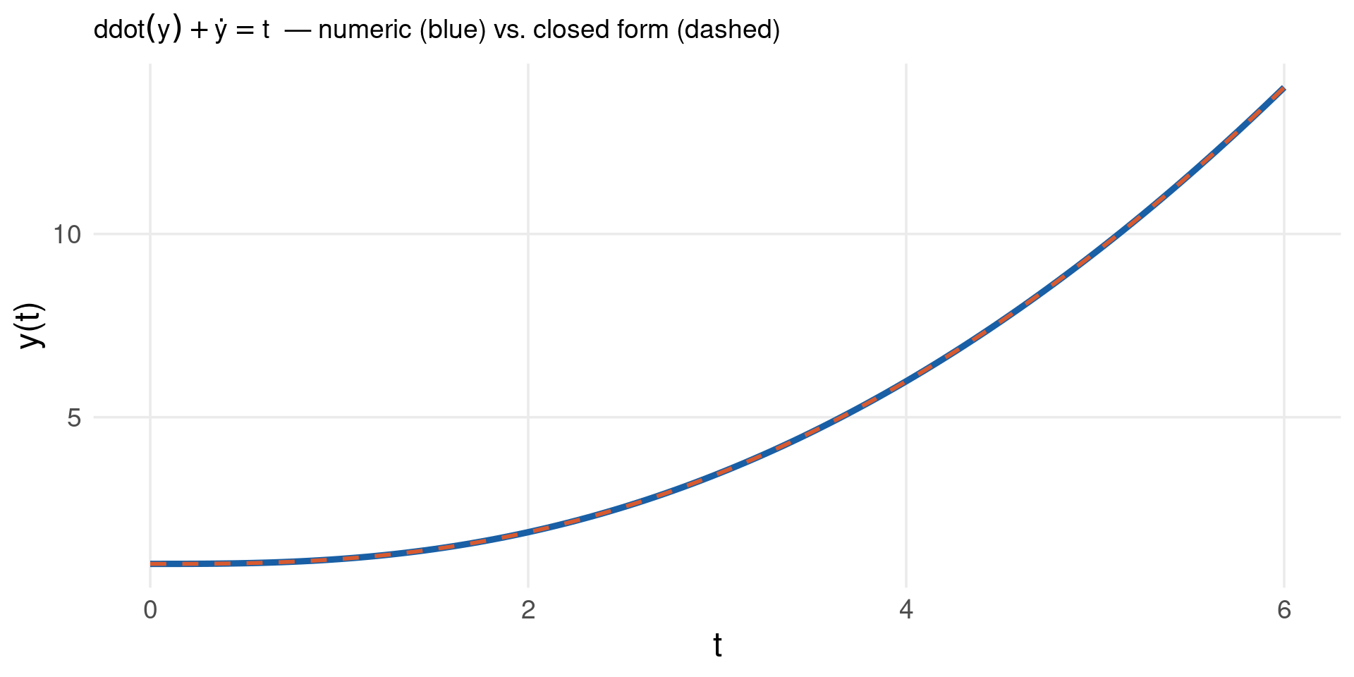
Code
# ÿ + ẏ = t   with y(0) = 1, ẏ(0) = 0
# Convert to first-order system: z1 = y, z2 = ẏ
rhs_nonhom <- function(t, z, parms) {
  list(c(z[2], t - z[2]))     # ż2 = g(t) - z2 = t - ẏ
}
sol_nonhom <- ode(y = c(y = 1, v = 0), times = seq(0, 6, by = 0.05),
                  func = rhs_nonhom, parms = NULL) %>%
  as.data.frame()

# Closed form: y(t) = c1 + c2*exp(-t) - t + 0.5*t^2
# Apply y(0)=1, ẏ(0)=0  ⇒  c1 + c2 = 1,  -c2 - 1 = 0 ⇒ c2 = -1, c1 = 2
exact_nonhom <- function(t) 2 - exp(-t) - t + 0.5 * t^2

sol_nonhom %>%
  ggplot() +
  aes(x = time) +
  geom_line(aes(y = y), color = col_main, linewidth = 1.6) +
  geom_line(data = data.frame(t = sol_nonhom$time, ex = exact_nonhom(sol_nonhom$time)),
            aes(x = t, y = ex), color = col_accent, linewidth = 1, linetype = "dashed") +
  labs(x = "t", y = "y(t)",
       title = expression(ddot(y) + dot(y) == t ~ " — numeric (blue) vs. closed form (dashed)")) +
  theme_lecture

Code
import sympy as sp
import numpy as np
import matplotlib.pyplot as plt

t = sp.Symbol("t")
y = sp.Function("y")

# ÿ + ẏ = t,  y(0)=1, ẏ(0)=0
ode_eq = sp.Eq(y(t).diff(t, 2) + y(t).diff(t), t)
sol = sp.dsolve(ode_eq, y(t), ics={y(0): 1, y(t).diff(t).subs(t, 0): 0})
print("Particular solution with y(0)=1, ẏ(0)=0:")
Particular solution with y(0)=1, ẏ(0)=0:
Code
sp.pprint(sol)
        2              
       t             -t
y(t) = -- - t + 2 - e  
       2               
Code
y_fn = sp.lambdify(t, sol.rhs, "numpy")
t_eval = np.linspace(0, 6, 300)

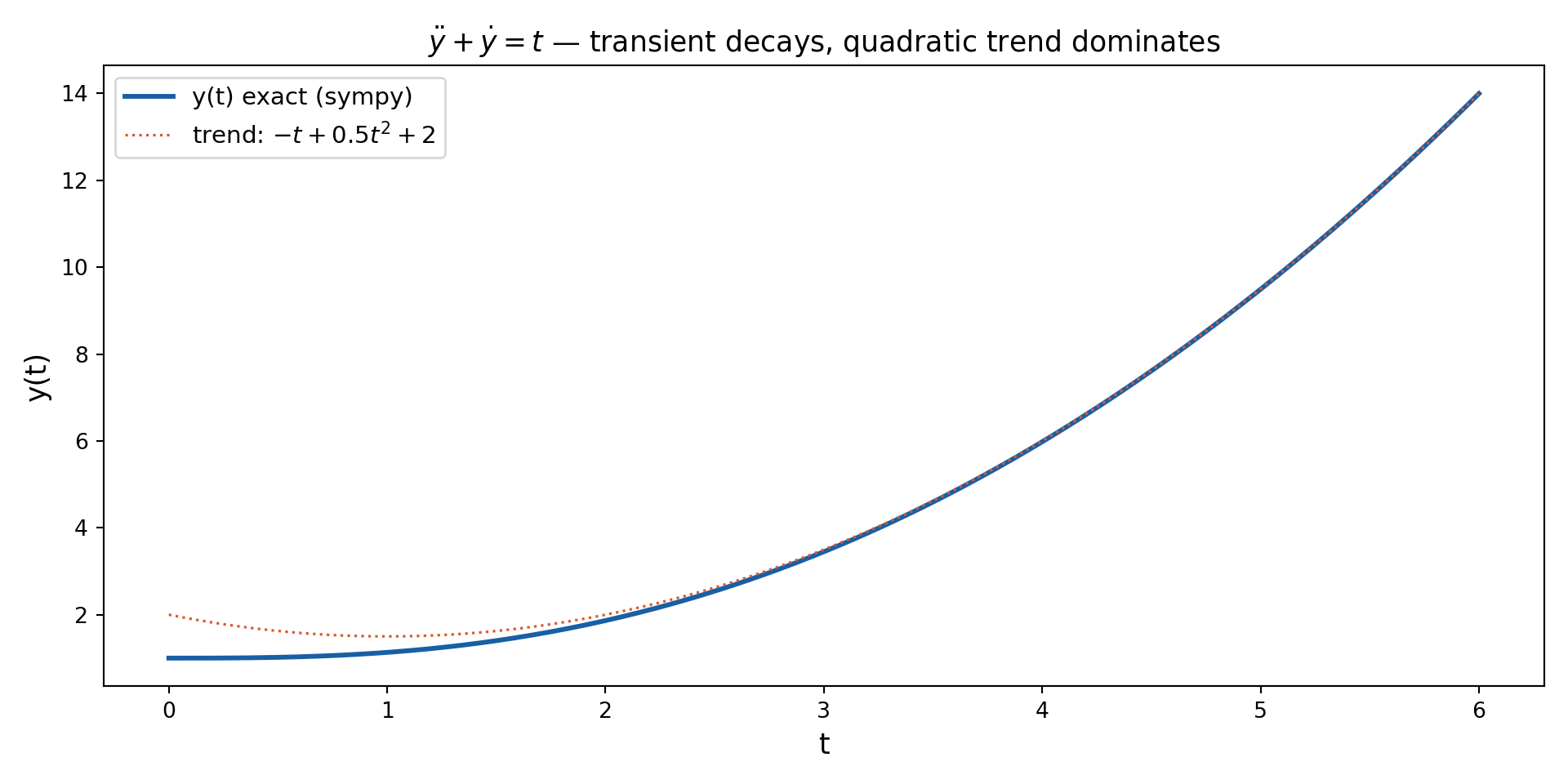
fig, ax = plt.subplots(figsize=(10, 5))
ax.plot(t_eval, y_fn(t_eval), color="#185FA5", linewidth=2.2, label="y(t) exact (sympy)")
ax.plot(t_eval, -t_eval + 0.5*t_eval**2 + 2, color="#D85A30",
        linewidth=1.2, linestyle="dotted", label=r"trend: $-t+0.5t^2+2$")
ax.set_xlabel("t", fontsize=13)
ax.set_ylabel("y(t)", fontsize=13)
ax.set_title(r"$\ddot{y}+\dot{y}=t$ — transient decays, quadratic trend dominates", fontsize=13)
ax.legend(fontsize=11)
plt.tight_layout()
plt.show()

Linearisation of Nonlinear ODEs & Liapunov’s Theorem

Problem: most economically-interesting ODEs \(\dot{x} = f(x)\) are nonlinear and have no closed-form solution. But we can still determine local stability near a fixed point.

Step 1 — find fixed points by solving \(f(x^*) = 0\) (there may be several).

Step 2 — Taylor-expand \(f\) around \(x^*\):

\[f(x) = f(x^*) + f'(x^*)(x-x^*) + \frac{f''(x^*)}{2!}(x-x^*)^2 + \cdots\]

Step 3 — truncate at first order. Since \(f(x^*) = 0\) by construction, and the remainder \(R_2(x,x^*) \approx 0\) when \(x\) is close to \(x^*\):

\[\boxed{f(x) \approx f'(x^*)\,(x - x^*)}\]

Step 4 — read off stability exactly as for a linear ODE \(\dot z = \lambda z\) with \(z = x-x^*\) and \(\lambda = f'(x^*)\):

\[x(t) \approx x^* + \bigl[x(0)-x^*\bigr]\,e^{f'(x^*)t}\]

\[f'(x^*) < 0 \Rightarrow \text{locally stable}, \qquad f'(x^*) > 0 \Rightarrow \text{locally unstable}\]

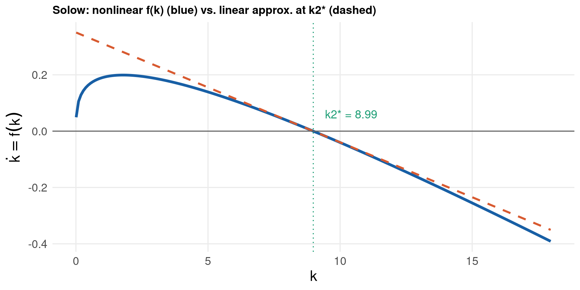
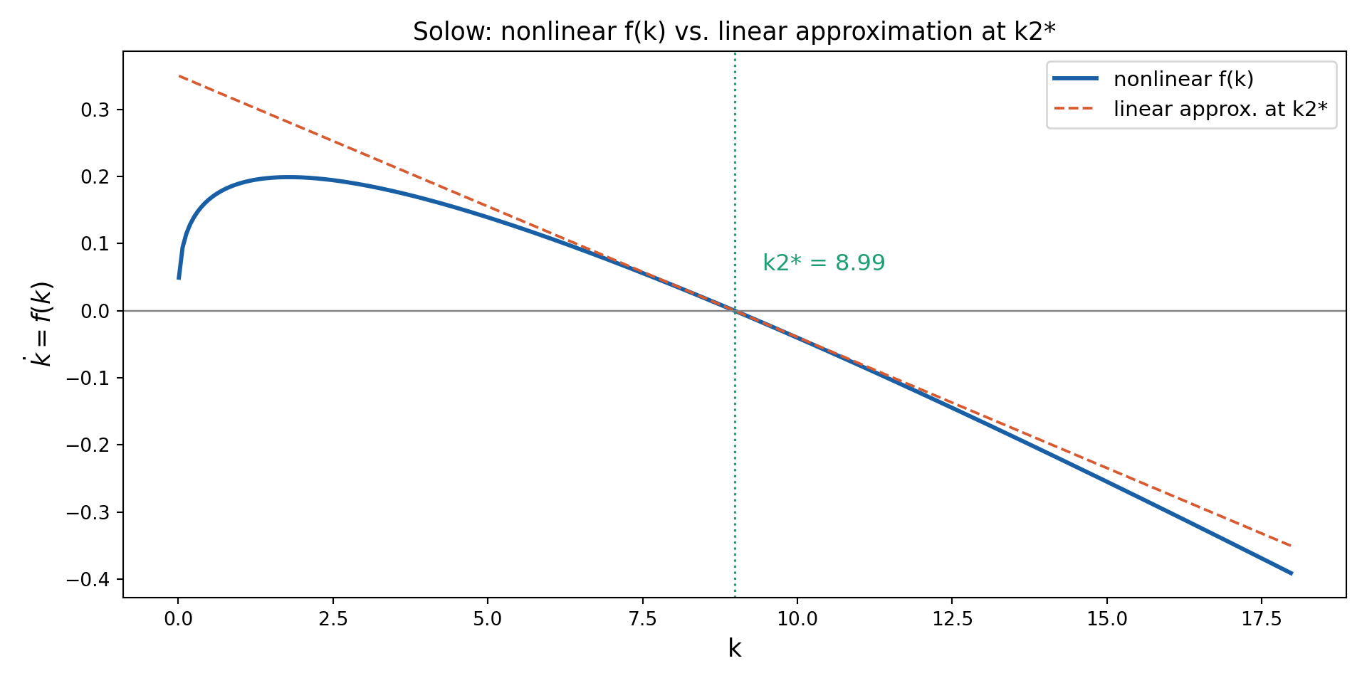
Solow growth model in continuous time:

\[\dot{k} = f(k) = sak^{\alpha} - (n+\delta)k\]

where \(k\) = capital per worker, \(s\) = savings rate, \(a\) = TFP, \(\alpha \in (0,1)\), \(n\) = population growth, \(\delta\) = depreciation.

Fixed points: factor out \(k\): \(k\bigl[sak^{\alpha-1}-(n+\delta)\bigr]=0\)

\[k_1^* = 0 \qquad\qquad k_2^* = \left(\frac{sa}{n+\delta}\right)^{1/(1-\alpha)}\]

Linearise at \(k_1^*=0\): \(f'(k) = \alpha sa\,k^{\alpha-1} - (n+\delta) \to \infty\) as \(k\to 0\) (since \(\alpha - 1 < 0\)) — the linear approximation breaks down at the origin.

Linearise at \(k_2^*>0\):

\[f'(k_2^*) = \alpha sa (k_2^*)^{\alpha-1} - (n+\delta) = \alpha(n+\delta) - (n+\delta) = -(n+\delta)(1-\alpha)\]

Since \(0<\alpha<1\) and \(n,\delta>0\): \(f'(k_2^*) < 0\) \(\Rightarrow\) \(k_2^*\) is locally stable.

Linear approximate solution near \(k_2^*\):

\[k(t) \approx k_2^* + \bigl[k(0)-k_2^*\bigr]\,e^{-(n+\delta)(1-\alpha)t} \xrightarrow{t\to\infty} k_2^*\]

Cautionary example: \(\dot{x} = f(x) = a(x-x^*)^3\), \(a<0\)

The unique fixed point \(x^*\) is globally stable: for \(x<x^*\), \((x-x^*)^3<0\) so \(\dot x = a(x-x^*)^3 > 0\) (moves right, toward \(x^*\)); for \(x>x^*\), \((x-x^*)^3>0\) so \(\dot x<0\) (moves left, toward \(x^*\)). Trajectories converge to \(x^*\) from both sides.

Linearise: \(f'(x) = 3a(x-x^*)^2 \Rightarrow f'(x^*) = 0\)

\[f(x) \approx f(x^*) + f'(x^*)(x-x^*) = 0\]

The linear approximation is \(\dot x = 0\) — a system that does not move at all, which is not stable in the usual asymptotic sense (any \(x_0 \neq x^*\) just stays at \(x_0\) forever under the linearised dynamics).

Code
s_p <- 0.25; a_p <- 1; alpha_p <- 0.35; n_p <- 0.02; delta_p <- 0.04

f_solow  <- function(k) s_p * a_p * k^alpha_p - (n_p + delta_p) * k
k2_star  <- (s_p * a_p / (n_p + delta_p))^(1 / (1 - alpha_p))
slope_at_k2 <- -(n_p + delta_p) * (1 - alpha_p)     # analytical f'(k2*)

k_grid <- seq(0.01, k2_star * 2, length.out = 200)

# True nonlinear ODE vs. its linear approximation around k2*
f_true   <- f_solow(k_grid)
f_linear <- slope_at_k2 * (k_grid - k2_star)

df_lin <- data.frame(k = k_grid, nonlinear = f_true, linear = f_linear)

df_lin %>%
  ggplot() +
  aes(x = k) +
  geom_line(aes(y = nonlinear), color = col_main,   linewidth = 1.6) +
  geom_line(aes(y = linear),    color = col_accent, linewidth = 1.2, linetype = "dashed") +
  geom_hline(yintercept = 0, color = "grey40") +
  geom_vline(xintercept = k2_star, linetype = "dotted", color = col_ok) +
  annotate("text", x = k2_star * 1.05, y = max(f_true) * 0.3,
           label = paste0("k2* = ", round(k2_star, 2)), color = col_ok, size = 5, hjust = 0) +
  labs(x = "k", y = expression(dot(k) == f(k)),
       title = "Solow: nonlinear f(k) (blue) vs. linear approx. at k2* (dashed)") +
  theme_lecture

Code
import numpy as np
import matplotlib.pyplot as plt

s, a, alpha, n, delta = 0.25, 1.0, 0.35, 0.02, 0.04

def f_solow(k):
    return s * a * k**alpha - (n + delta) * k

k2_star = (s * a / (n + delta)) ** (1 / (1 - alpha))
slope_k2 = -(n + delta) * (1 - alpha)          # analytical f'(k2*)

k_grid = np.linspace(0.01, k2_star * 2, 300)
f_true   = f_solow(k_grid)
f_linear = slope_k2 * (k_grid - k2_star)

fig, ax = plt.subplots(figsize=(10, 5))
ax.plot(k_grid, f_true,   color="#185FA5", linewidth=2.2, label="nonlinear f(k)")
ax.plot(k_grid, f_linear, color="#D85A30", linewidth=1.4,
        linestyle="--",  label="linear approx. at k2*")
ax.axhline(0, color="grey", linewidth=0.9)
ax.axvline(k2_star, color="#1D9E75", linestyle=":", linewidth=1.2)
ax.text(k2_star * 1.05, max(f_true) * 0.3, f"k2* = {k2_star:.2f}",
        color="#1D9E75", fontsize=12)
ax.set_xlabel("k", fontsize=13)
ax.set_ylabel(r"$\dot{k} = f(k)$", fontsize=13)
ax.set_title("Solow: nonlinear f(k) vs. linear approximation at k2*", fontsize=13)
ax.legend(fontsize=11)
plt.tight_layout()
plt.show()

Continuous ODE Code

Code
rhs   <- function(t, y, parms) list(parms$a + parms$b * y[1])
parms <- list(a = 4, b = -2)   # ẋ = 4 - 2x → x* = 2
sol   <- ode(y = c(x = 0.1), times = seq(0, 5, by = 0.05),
             func = rhs, parms = parms)

as.data.frame(sol) %>%
  ggplot() +
  aes(x = time, y = x) +
  geom_line(color = col_main, linewidth = 1.2) +
  geom_hline(yintercept = 2, linetype = "dashed", color = col_accent) +
  annotate("text", x = 4, y = 2.1, label = "x* = 2", color = col_accent) +
  labs(x = "t", y = "x(t)", title = expression(dot(x) == 4 - 2*x)) +
  theme_lecture

Code
logistic_rhs <- function(t, y, parms) {
  list(parms$alpha * y[1] * (1 - y[1] / parms$K))
}
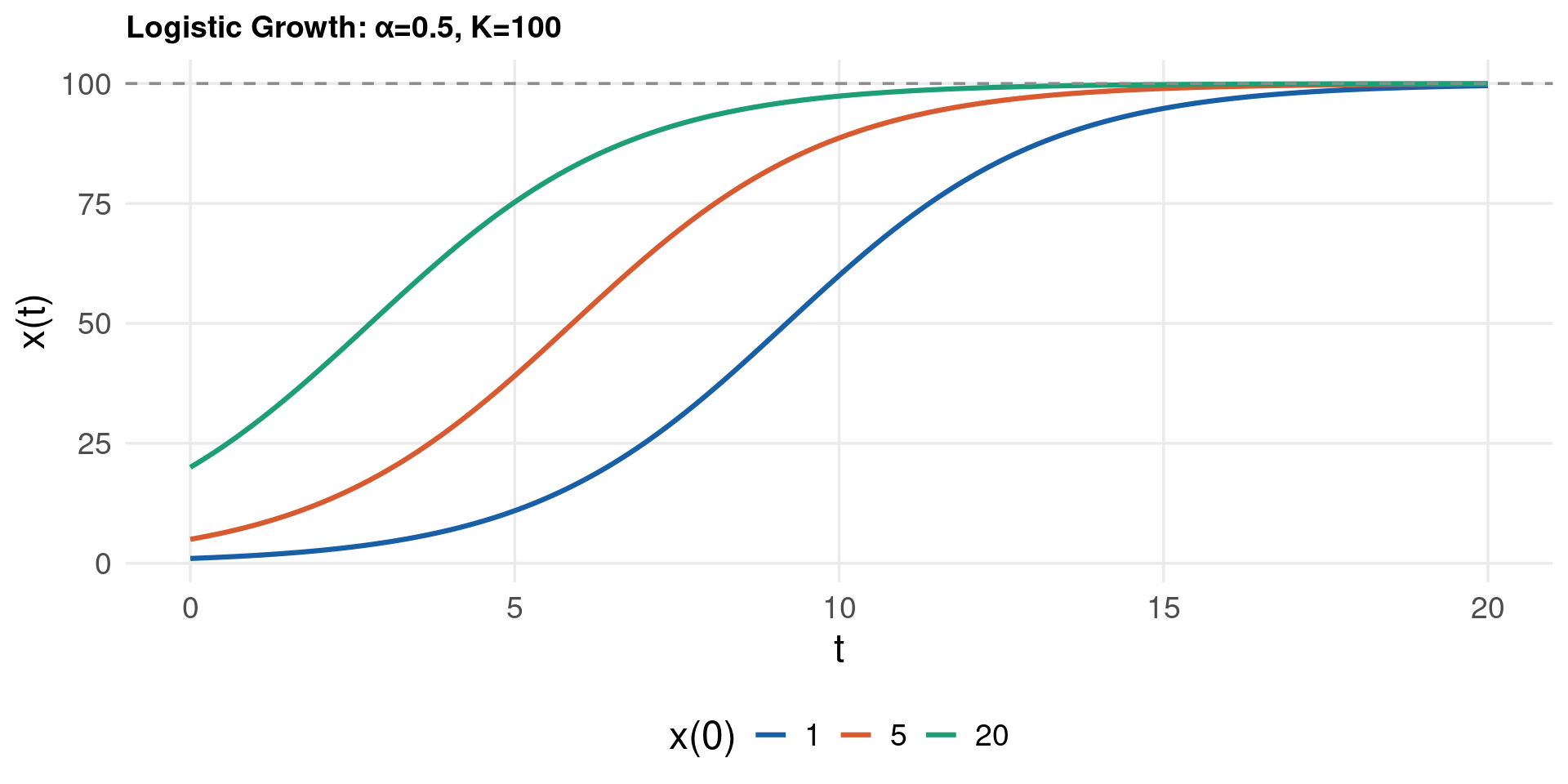
parms <- list(alpha = 0.5, K = 100)
inits <- c(1, 5, 20)
cols  <- c(col_main, col_accent, col_ok)

sols <- lapply(inits, function(x0) {
  ode(y = c(x = x0), times = seq(0, 20, by = 0.1),
      func = logistic_rhs, parms = parms) %>%
    as.data.frame() %>%
    mutate(x0 = x0)
})

bind_rows(sols) %>%
  ggplot() +
  aes(x = time, y = x, color = factor(x0)) +
  geom_line(linewidth = 1.1) +
  geom_hline(yintercept = 100, linetype = "dashed", color = col_muted) +
  scale_color_manual(values = cols, name = "x(0)") +
  labs(x = "t", y = "x(t)", title = "Logistic Growth: α=0.5, K=100") +
  theme_lecture

Code
import numpy as np
import matplotlib.pyplot as plt
from scipy.integrate import solve_ivp

def logistic(t, y, alpha, K):
    return [alpha * y[0] * (1 - y[0] / K)]

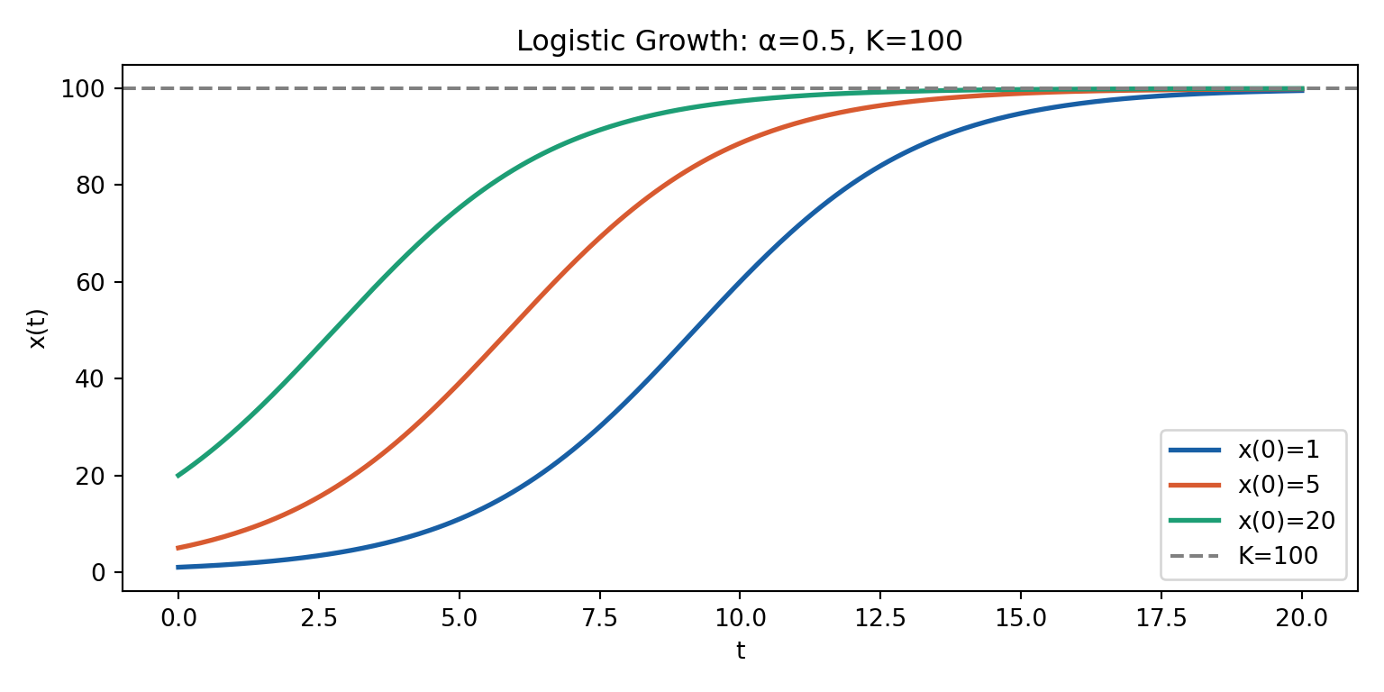
alpha, K = 0.5, 100
t_eval = np.linspace(0, 20, 300)
colors = ["#185FA5", "#D85A30", "#1D9E75"]
inits  = [1, 5, 20]

fig, ax = plt.subplots(figsize=(8, 4))
for x0, c in zip(inits, colors):
    sol = solve_ivp(logistic, (0, 20), [x0], args=(alpha, K), t_eval=t_eval)
    ax.plot(sol.t, sol.y[0], color=c, linewidth=2, label=f"x(0)={x0}")
ax.axhline(K, linestyle="--", color="grey", label="K=100")
ax.set_xlabel("t"); ax.set_ylabel("x(t)")
ax.set_title("Logistic Growth: α=0.5, K=100")
ax.legend(); plt.tight_layout(); plt.show()

Phase Portrait — Concepts & Construction

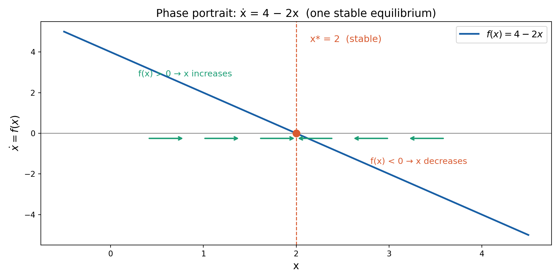
A phase portrait (or phase line for a scalar ODE) answers the question: without solving the ODE, what will \(x(t)\) do?

Construction — three steps:

  1. Draw \(f(x)\) vs \(x\) — horizontal axis is \(x\), vertical axis is \(\dot{x} = f(x)\)
  2. Mark equilibria — where \(f(x^*) = 0\), i.e. the curve crosses the \(x\)-axis
  3. Add direction arrows on the \(x\)-axis:
    • \(f(x) > 0\) (curve above axis) \(\Rightarrow\) \(\dot{x} > 0\) \(\Rightarrow\) \(x\) increases \(\Rightarrow\) arrow right
    • \(f(x) < 0\) (curve below axis) \(\Rightarrow\) \(\dot{x} < 0\) \(\Rightarrow\) \(x\) decreases \(\Rightarrow\) arrow left

Stability directly from the slope of \(f\) at \(x^*\):

\[f'(x^*) < 0 \;\Rightarrow\; \text{arrows point toward } x^* \;\Rightarrow\; \textbf{stable (attractor)}\]

\[f'(x^*) > 0 \;\Rightarrow\; \text{arrows point away from } x^* \;\Rightarrow\; \textbf{unstable (repeller)}\]

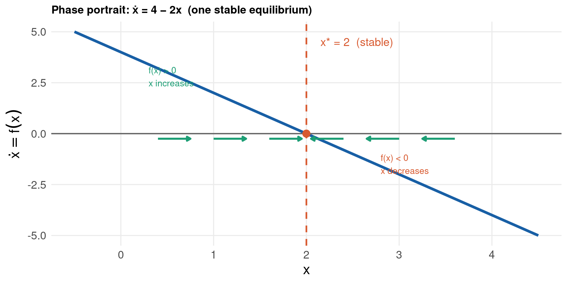
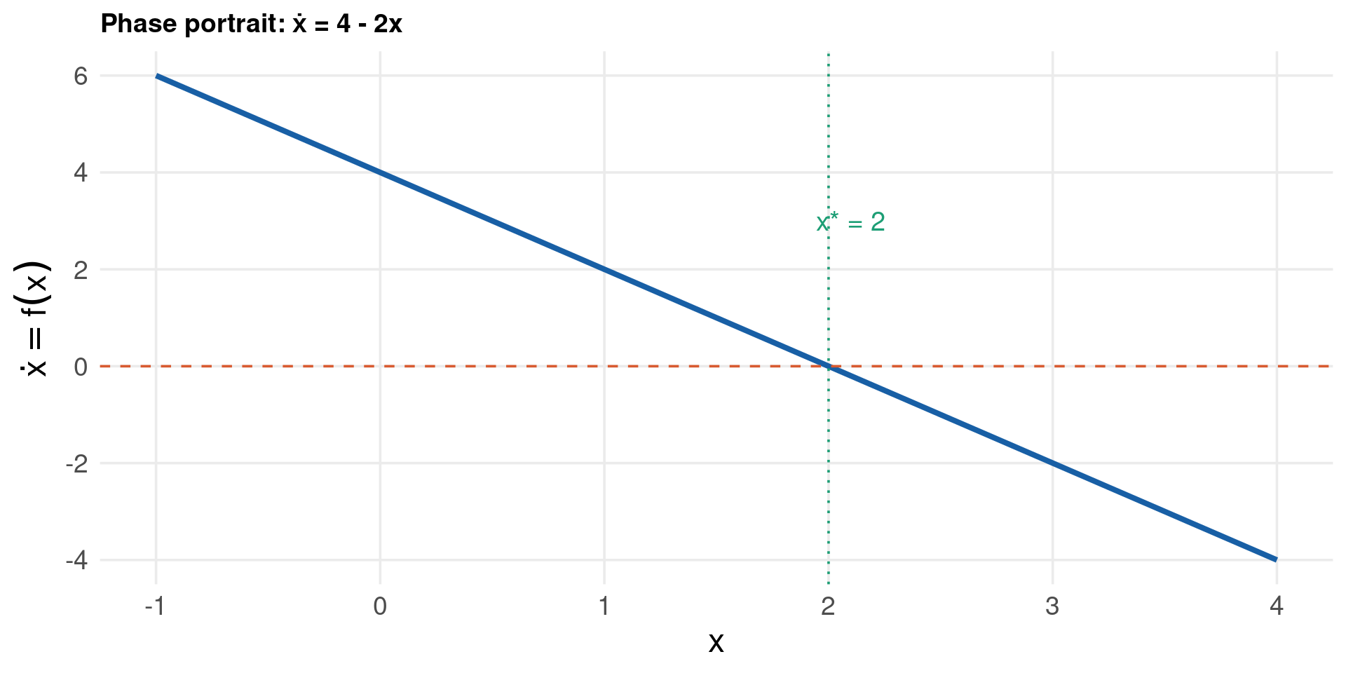
Example: \(\dot{x} = 4 - 2x\), so \(f(x) = 4 - 2x\)

Region \(f(x)\) sign Direction Conclusion
\(x < 2\) \(+\) right moving toward \(x^*\)
\(x = 2\) \(0\) equilibrium \(x^* = 2\)
\(x > 2\) \(-\) left moving toward \(x^*\)

Since arrows converge from both sides, \(x^* = 2\) is globally stable.

Slope at equilibrium: \(f'(x) = -2 < 0\) — confirms stability.

Key read-offs from the phase portrait: - The \(x\)-intercept gives \(x^*\) immediately - The sign of the slope of \(f\) at the crossing tells you stability - The distance of the curve from zero tells you how fast \(x\) moves

Code
xv    <- seq(-0.5, 4.5, by = 0.05)
f_val <- 4 - 2 * xv          # f(x) = 4 - 2x

# Direction arrows on the x-axis
arrow_x <- c(0.4, 1.0, 1.6, 2.4, 3.0, 3.6)
arrow_dx <- ifelse(4 - 2 * arrow_x > 0, 0.35, -0.35)

ggplot() +
  aes(x = xv, y = f_val) +
  geom_line(data = data.frame(xv, f_val),
            color = col_main, linewidth = 1.6) +
  geom_hline(yintercept = 0, color = "grey40", linewidth = 0.8) +
  geom_vline(xintercept = 2, linetype = "dashed", color = col_accent, linewidth = 1) +
  geom_segment(
    data = data.frame(x = arrow_x, xend = arrow_x + arrow_dx, y = -0.25, yend = -0.25),
    aes(x = x, xend = xend, y = y, yend = yend),
    arrow = arrow(type = "closed", length = unit(0.18, "cm")),
    color = col_ok, linewidth = 1.2
  ) +
  geom_point(aes(x = 2, y = 0), color = col_accent, size = 4) +
  annotate("text", x = 2.15, y = 4.5,
           label = "x* = 2  (stable)", color = col_accent, size = 5, hjust = 0) +
  annotate("text", x = 0.3,  y = 2.8,
           label = "f(x) > 0\nx increases", color = col_ok, size = 4, hjust = 0) +
  annotate("text", x = 2.8,  y = -1.5,
           label = "f(x) < 0\nx decreases", color = col_accent, size = 4, hjust = 0) +
  labs(x = "x", y = expression(dot(x) == f(x)),
       title = "Phase portrait: ẋ = 4 − 2x  (one stable equilibrium)") +
  theme_lecture

Code
import numpy as np
import matplotlib.pyplot as plt
import matplotlib.patches as mpatches

x   = np.linspace(-0.5, 4.5, 300)
fx  = 4 - 2 * x

fig, ax = plt.subplots(figsize=(10, 5))
ax.plot(x, fx, color="#185FA5", linewidth=2.2, label=r"$f(x) = 4 - 2x$")
ax.axhline(0,  color="grey",    linewidth=0.9)
ax.axvline(2,  color="#D85A30", linewidth=1.2, linestyle="--")
ax.plot(2, 0, "o", color="#D85A30", markersize=9, zorder=5)

# Direction arrows on the x-axis
for xa in [0.4, 1.0, 1.6, 2.4, 3.0, 3.6]:
    dx = 0.4 if (4 - 2*xa) > 0 else -0.4
    ax.annotate("", xy=(xa + dx, -0.25), xytext=(xa, -0.25),
                arrowprops=dict(arrowstyle="->", color="#1D9E75", lw=1.8))

ax.text(2.15, 4.5, "x* = 2  (stable)", color="#D85A30", fontsize=12)
ax.text(0.3,  2.8, "f(x) > 0 → x increases", color="#1D9E75", fontsize=11)
ax.text(2.8, -1.5, "f(x) < 0 → x decreases", color="#D85A30", fontsize=11)
ax.set_xlabel("x", fontsize=13)
ax.set_ylabel(r"$\dot{x} = f(x)$", fontsize=13)
ax.set_title("Phase portrait: ẋ = 4 − 2x  (one stable equilibrium)", fontsize=14)
ax.legend(fontsize=12)
plt.tight_layout()
plt.show()

Phase Portrait — Multiple Equilibria

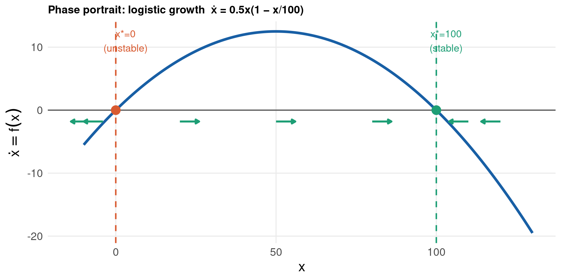
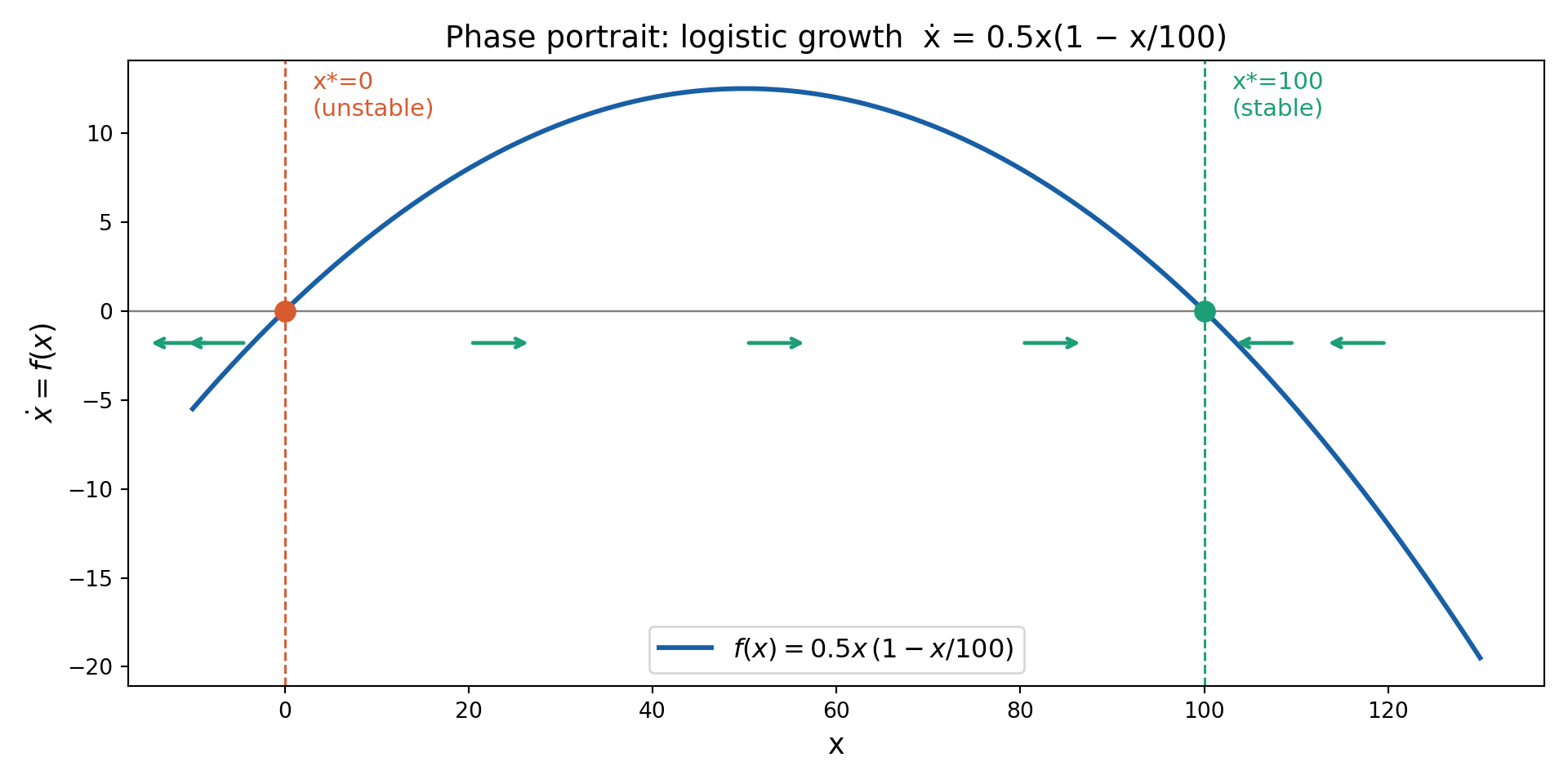
Nonlinear \(f(x)\) can cross zero multiple times — each crossing is an equilibrium. Stability alternates with the sign of the slope.

Example — logistic model: \(\dot{x} = rx\!\left(1 - \dfrac{x}{K}\right)\), \(r = 0.5\), \(K = 100\)

\[f(x) = 0.5\,x\!\left(1 - \frac{x}{100}\right)\]

Two equilibria: \(x^* = 0\) and \(x^* = 100\).

Equilibrium \(f'(x^*)\) Stability Interpretation
\(x^* = 0\) \(+0.5 > 0\) Unstable extinction repeller
\(x^* = 100\) \(-0.5 < 0\) Stable carrying capacity attractor

Basin of attraction: all \(x_0 > 0\) converge to \(K = 100\); \(x_0 < 0\) is infeasible here.

Generalisation: for any smooth \(f\): - zeros alternate between stable and unstable (under generic conditions) - stable equilibria are separated by unstable ones (the unstable ones act as thresholds) - the unstable equilibrium defines the boundary between basins of attraction

Code
r_l <- 0.5; K_l <- 100
xv_m  <- seq(-10, 130, by = 0.5)
fv_m  <- r_l * xv_m * (1 - xv_m / K_l)

# Arrow positions and directions
ax_m  <- c(-8, -4, 20, 50, 80, 110, 120)
adx_m <- ifelse(r_l * ax_m * (1 - ax_m / K_l) > 0, 6, -6)

# Labels for equilibrium stability
eq_pts <- data.frame(
  x     = c(0,         100),
  label = c("x*=0\n(unstable)", "x*=100\n(stable)"),
  col   = c(col_accent, col_ok)
)

ggplot() +
  geom_line(data = data.frame(x = xv_m, y = fv_m),
            aes(x = x, y = y), color = col_main, linewidth = 1.6) +
  geom_hline(yintercept = 0, color = "grey40", linewidth = 0.8) +
  geom_segment(
    data = data.frame(x = ax_m, xend = ax_m + adx_m, y = -1.8, yend = -1.8),
    aes(x = x, xend = xend, y = y, yend = yend),
    arrow = arrow(type = "closed", length = unit(0.18, "cm")),
    color = col_ok, linewidth = 1.2
  ) +
  geom_point(data = eq_pts, aes(x = x, y = 0, color = col), size = 5) +
  scale_color_identity() +
  geom_vline(xintercept = 0,   linetype = "dashed", color = col_accent, linewidth = 0.9) +
  geom_vline(xintercept = 100, linetype = "dashed", color = col_ok,     linewidth = 0.9) +
  annotate("text", x =  3,  y = 11, label = "x*=0\n(unstable)", color = col_accent, size = 4.5) +
  annotate("text", x = 103, y = 11, label = "x*=100\n(stable)",  color = col_ok,     size = 4.5) +
  labs(x = "x", y = expression(dot(x) == f(x)),
       title = "Phase portrait: logistic growth  ẋ = 0.5x(1 − x/100)") +
  theme_lecture

Code
import numpy as np
import matplotlib.pyplot as plt

r_l, K_l = 0.5, 100.0
x   = np.linspace(-10, 130, 400)
fx  = r_l * x * (1 - x / K_l)

fig, ax = plt.subplots(figsize=(10, 5))
ax.plot(x, fx, color="#185FA5", linewidth=2.2,
        label=r"$f(x) = 0.5x\,(1 - x/100)$")
ax.axhline(0, color="grey", linewidth=0.9)

# Equilibrium verticals
ax.axvline(0,   color="#D85A30", linewidth=1.1, linestyle="--")
ax.axvline(100, color="#1D9E75", linewidth=1.1, linestyle="--")
ax.plot([0, 100], [0, 0], "o", color=["#D85A30", "#1D9E75"]
        if False else "#185FA5", markersize=1)   # dummy — draw separately
ax.plot(0,   0, "o", color="#D85A30", markersize=9, zorder=5)
ax.plot(100, 0, "o", color="#1D9E75", markersize=9, zorder=5)

# Direction arrows
for xa in [-8, -4, 20, 50, 80, 110, 120]:
    dval = r_l * xa * (1 - xa / K_l)
    dx   = 7 if dval > 0 else -7
    ax.annotate("", xy=(xa + dx, -1.8), xytext=(xa, -1.8),
                arrowprops=dict(arrowstyle="->", color="#1D9E75", lw=1.8))

ax.text(3,   11, "x*=0\n(unstable)", color="#D85A30", fontsize=11)
ax.text(103, 11, "x*=100\n(stable)", color="#1D9E75", fontsize=11)
ax.set_xlabel("x", fontsize=13)
ax.set_ylabel(r"$\dot{x} = f(x)$", fontsize=13)
ax.set_title("Phase portrait: logistic growth  ẋ = 0.5x(1 − x/100)", fontsize=14)
ax.legend(fontsize=12)
plt.tight_layout()
plt.show()

Harrod-Domar & Phase Portrait Code

Code
hd_rhs <- function(t, y, parms) list(parms$g * y[1])
g_w <- 0.03   # warranted growth rate = s/v = 0.15/5

sols_hd <- lapply(c(0.5, 1.0, 2.0), function(y0) {
  ode(y = c(Y = y0), times = seq(0, 50, by = 0.5),
      func = hd_rhs, parms = list(g = g_w)) %>%
    as.data.frame() %>%
    mutate(Y0 = y0)
})

bind_rows(sols_hd) %>%
  ggplot() +
  aes(x = time, y = Y, color = factor(Y0)) +
  geom_line(linewidth = 1.1) +
  scale_color_manual(values = c(col_main, col_accent, col_ok), name = "Y(0)") +
  labs(x = "t", y = "Y(t)",
       title = glue("Harrod-Domar: Ẏ = {g_w}Y  (s=0.15, v=5)")) +
  theme_lecture

Code
xv     <- seq(-1, 4, by = 0.05)
f_pp   <- function(x) 4 - 2*x   # ẋ = 4 - 2x

p1 <- ggplot(data.frame(x = xv, dx = f_pp(xv))) +
  aes(x = x, y = dx) +
  geom_line(color = col_main, linewidth = 1.4) +
  geom_hline(yintercept = 0, linetype = "dashed", color = col_accent) +
  geom_vline(xintercept = 2, linetype = "dotted", color = col_ok) +
  annotate("text", x = 2.1, y = 3, label = "x* = 2", color = col_ok, size = 5) +
  labs(x = "x", y = expression(dot(x) == f(x)),
       title = "Phase portrait: ẋ = 4 - 2x") +
  theme_lecture

p1

Code
import numpy as np
import matplotlib.pyplot as plt
from scipy.integrate import solve_ivp

g_w = 0.03
t_eval = np.linspace(0, 50, 300)
y0s    = [0.5, 1.0, 2.0]
colors = ["#185FA5", "#D85A30", "#1D9E75"]

fig, axes = plt.subplots(1, 2, figsize=(10, 5))
for y0, c in zip(y0s, colors):
    sol = solve_ivp(lambda t, y: [g_w * y[0]], [0, 50], [y0], t_eval=t_eval)
    axes[0].plot(sol.t, sol.y[0], color=c, linewidth=2, label=f"Y(0)={y0}")
axes[0].set_xlabel("t"); axes[0].set_ylabel("Y(t)")
axes[0].set_title(f"Harrod-Domar: g_w={g_w}")
axes[0].legend()

x = np.linspace(-1, 4, 200)
axes[1].plot(x, 4 - 2*x, color="#185FA5", linewidth=2)
axes[1].axhline(0, linestyle="--", color="#D85A30")
axes[1].axvline(2, linestyle=":", color="#1D9E75")
axes[1].set_xlabel("x"); axes[1].set_ylabel("ẋ = f(x)")
axes[1].set_title("Phase portrait: ẋ = 4 - 2x")
plt.tight_layout(); plt.show()

Part III: Discrete Dynamic Systems

Difference equations, cobweb, Solow, business cycles

The Cobweb Theorem

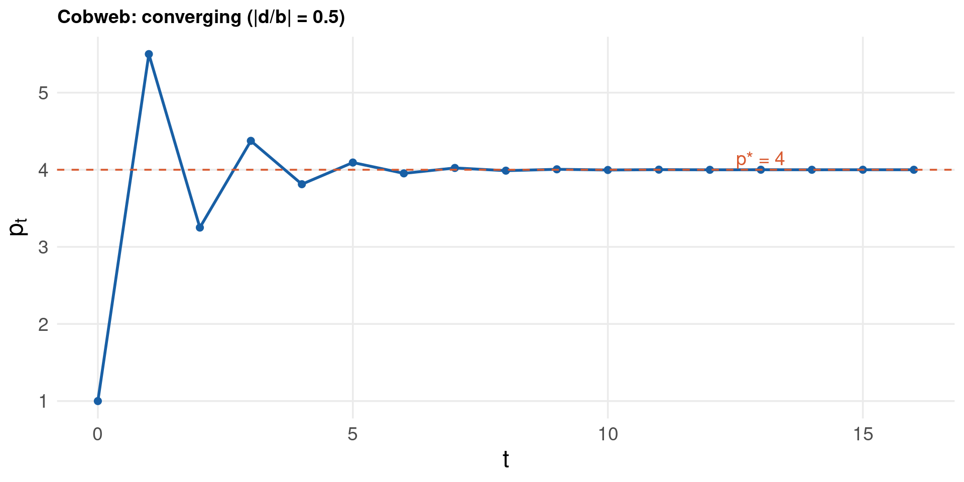
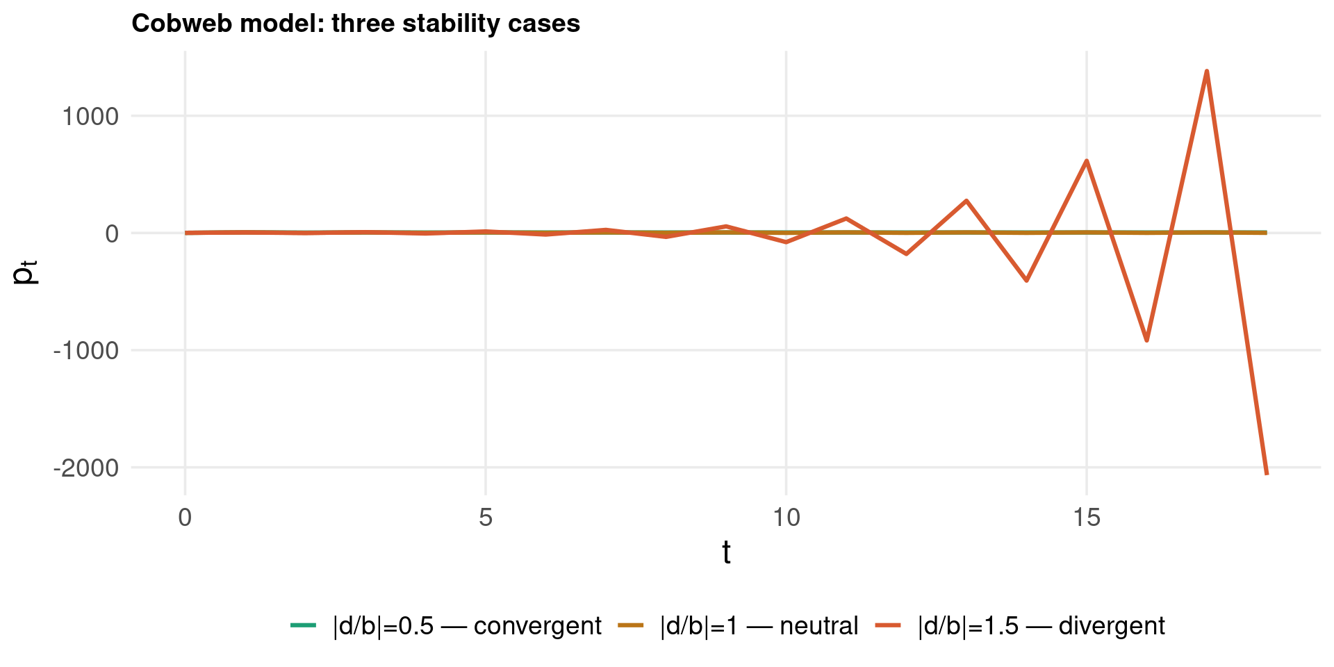
\[q^d_t = a - b p_t \quad \text{(demand, current price)}\] \[q^s_t = c + d p_{t-1} \quad \text{(supply, lagged price)}\]

Market clearing \(q^d_t = q^s_t\):

\[p_t = \frac{a-c}{b+d} - \frac{d}{b} p_{t-1}\]

Fixed point: \(p^* = (a-c)/(b+d)\)

Stability: \(|{-d/b}| < 1\), i.e., \(d < b\)

Producers base supply on last period’s price; demand responds to current price.

\(|d/b|\) Behaviour
\(< 1\) converging cobweb
\(= 1\) perpetual oscillation
\(> 1\) diverging cobweb

Discrete Logistic, Multiplier-Accelerator & Solow

\[x_t = \lambda x_{t-1}(1 - x_{t-1})\]

For \(\lambda = 3.5\): period-4 attractor (see Part VII for full bifurcation diagram).

Compound interest: \(A_n = A_0(1+r)^n\)

Second-order linear: \(x_t = a_1 x_{t-1} + a_2 x_{t-2} + b\); characteristic roots determine oscillations and stability.

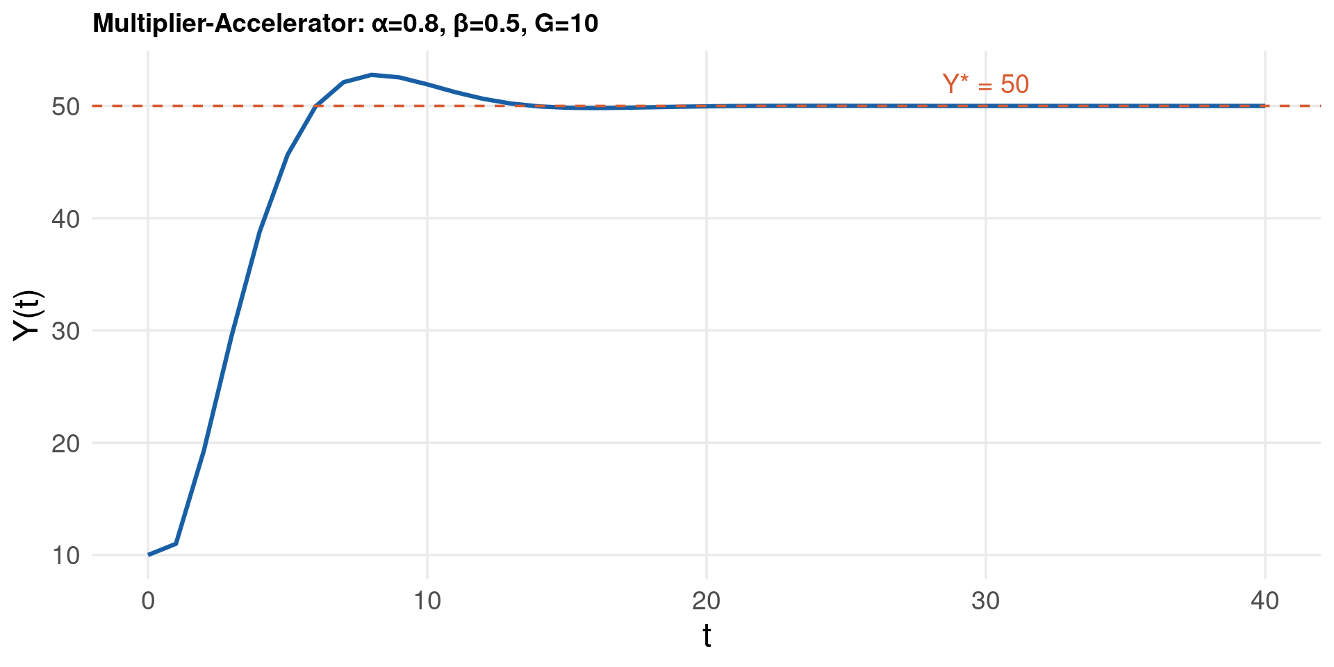
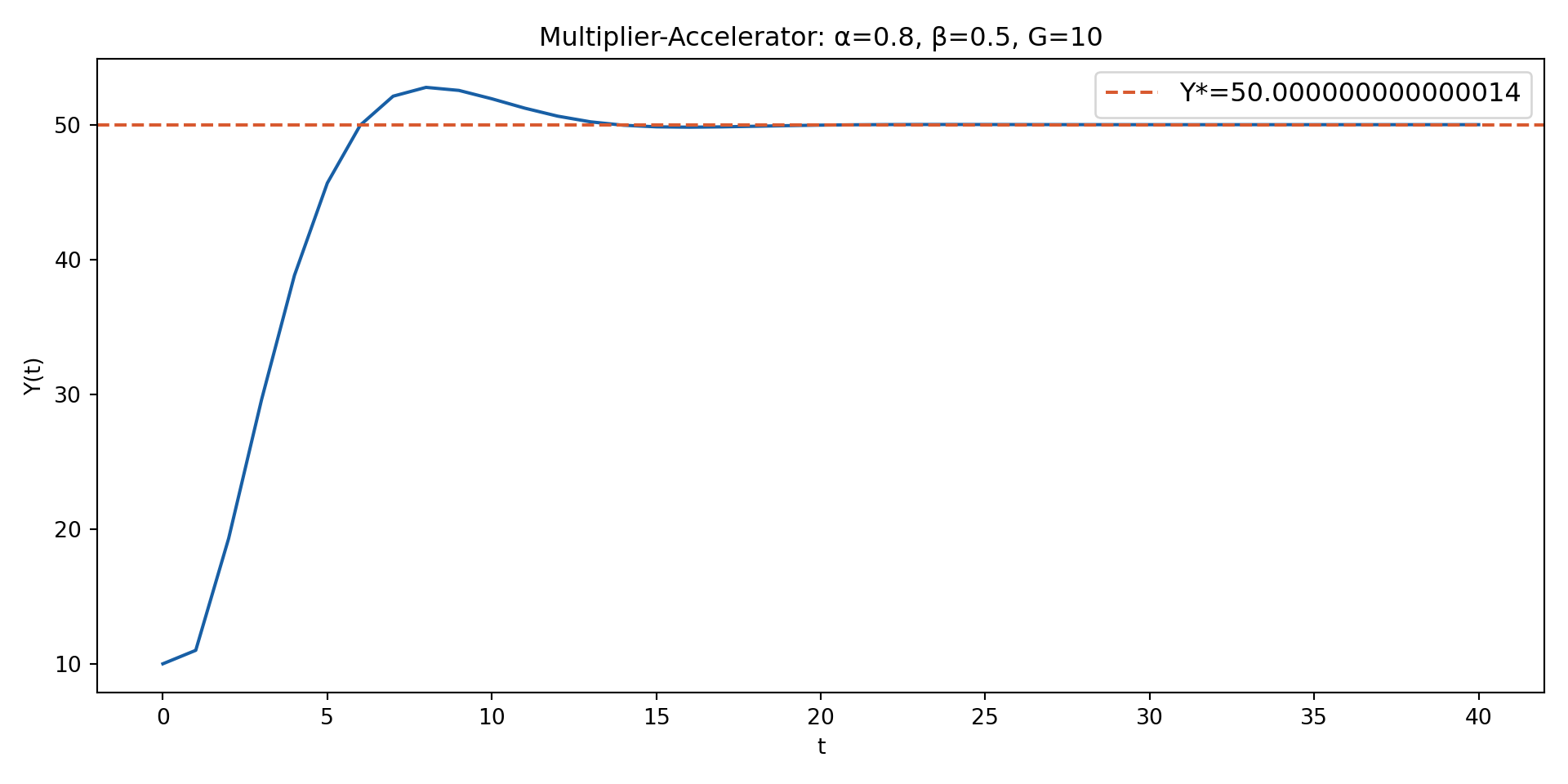
\[Y_t = C_t + I_t + G\]

  • Consumption: \(C_t = \alpha Y_{t-1}\), \(0 < \alpha < 1\)
  • Investment: \(I_t = \beta(Y_{t-1} - Y_{t-2})\), \(\beta > 0\)

\[Y_t = (\alpha + \beta)Y_{t-1} - \beta Y_{t-2} + G\]

Equilibrium: \(Y^* = G/(1-\alpha)\)

Oscillations possible for \(\beta > (1-\alpha)^2/(4\alpha)\).

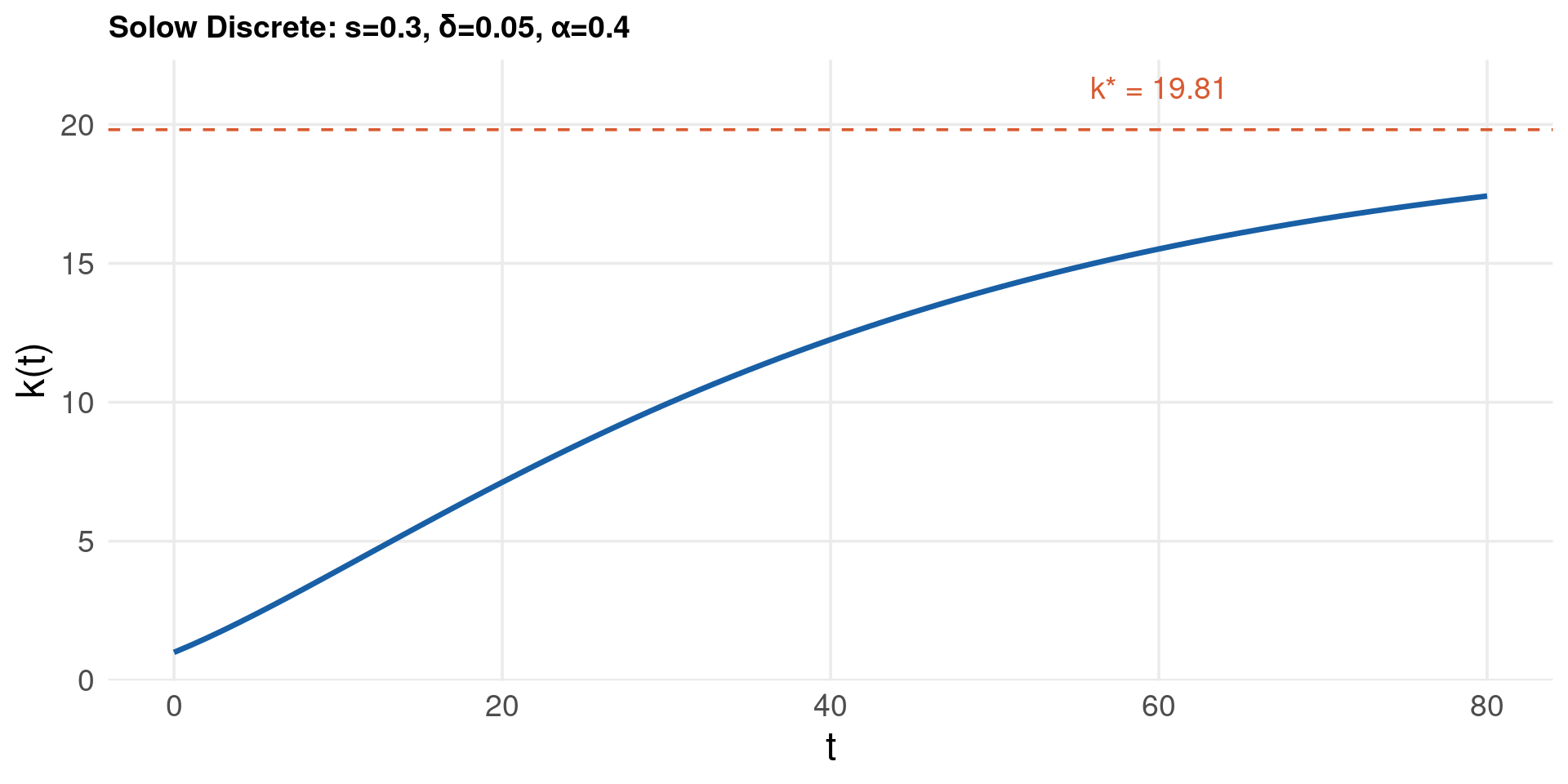
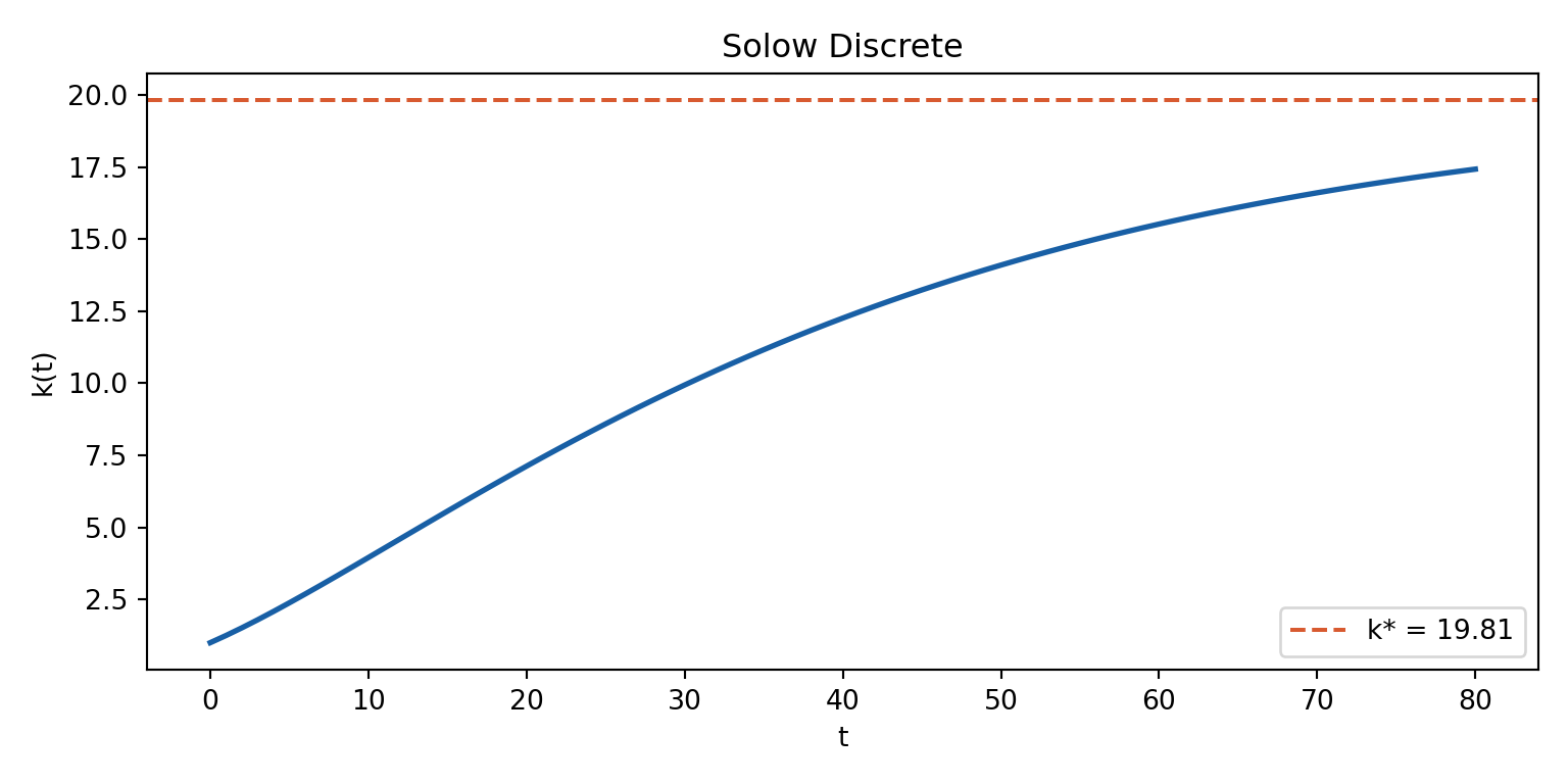
\[k_{t+1} = s k_t^\alpha + (1-\delta) k_t\]

Steady state: \(s(k^*)^\alpha = \delta k^*\)

\[k^* = \left(\frac{s}{\delta}\right)^{1/(1-\alpha)}\]

Global convergence: \(k_t \to k^*\) from any \(k_0 > 0\).

Discrete Dynamics Code

Code
a <- 10; b <- 2; cc <- -2; d <- 1   # |d/b| = 0.5 → converging
p_star <- (a - cc) / (b + d)
T  <- 16
pt <- numeric(T + 1); pt[1] <- 1.0
for (t in seq_len(T)) pt[t+1] <- (a - cc - d * pt[t]) / b

data.frame(t = 0:T, p = pt) %>%
  ggplot() +
  aes(x = t, y = p) +
  geom_line(color = col_main, linewidth = 1) +
  geom_point(color = col_main, size = 2) +
  geom_hline(yintercept = p_star, linetype = "dashed", color = col_accent) +
  annotate("text", x = 13, y = p_star + 0.15,
           label = glue("p* = {round(p_star,2)}"), color = col_accent) +
  labs(x = "t", y = expression(p[t]),
       title = "Cobweb: converging (|d/b| = 0.5)") +
  theme_lecture

Code
s <- 0.3; delta <- 0.05; alpha <- 0.4
k_star <- (s / delta)^(1 / (1 - alpha))
T  <- 80
k  <- numeric(T + 1); k[1] <- 1.0
for (t in seq_len(T)) k[t+1] <- s * k[t]^alpha + (1 - delta) * k[t]

data.frame(t = 0:T, k = k) %>%
  ggplot() +
  aes(x = t, y = k) +
  geom_line(color = col_main, linewidth = 1.2) +
  geom_hline(yintercept = k_star, linetype = "dashed", color = col_accent) +
  annotate("text", x = 60, y = k_star + 1.5,
           label = glue("k* = {round(k_star,2)}"), color = col_accent) +
  labs(x = "t", y = "k(t)",
       title = "Solow Discrete: s=0.3, δ=0.05, α=0.4") +
  theme_lecture

Code
import numpy as np
import matplotlib.pyplot as plt

s, delta, alpha = 0.3, 0.05, 0.4
k_star = (s / delta)**(1 / (1 - alpha))
T = 80
k = np.zeros(T + 1); k[0] = 1.0
for t in range(T):
    k[t+1] = s * k[t]**alpha + (1 - delta) * k[t]

fig, ax = plt.subplots(figsize=(8, 4))
ax.plot(range(T+1), k, color="#185FA5", linewidth=2)
ax.axhline(k_star, linestyle="--", color="#D85A30",
           label=f"k* = {k_star:.2f}")
ax.set_xlabel("t"); ax.set_ylabel("k(t)")
ax.set_title("Solow Discrete")
ax.legend(); plt.tight_layout(); plt.show()

Multiplier-Accelerator & Cobweb Code

Code
alpha_ma <- 0.8; beta_ma <- 0.5; G_ma <- 10
Y_star   <- G_ma / (1 - alpha_ma)
T_ma <- 40
Y_ma <- numeric(T_ma + 1)
Y_ma[1] <- 10; Y_ma[2] <- 11

for (t in 2:T_ma)
  Y_ma[t+1] <- (alpha_ma + beta_ma)*Y_ma[t] - beta_ma*Y_ma[t-1] + G_ma

data.frame(t = 0:T_ma, Y = Y_ma) %>%
  ggplot() +
  aes(x = t, y = Y) +
  geom_line(color = col_main, linewidth = 1.1) +
  geom_hline(yintercept = Y_star, linetype = "dashed", color = col_accent) +
  annotate("text", x = 30, y = Y_star + 2,
           label = glue("Y* = {Y_star}"), color = col_accent, size = 5) +
  labs(x = "t", y = "Y(t)",
       title = glue("Multiplier-Accelerator: α={alpha_ma}, β={beta_ma}, G={G_ma}")) +
  theme_lecture

Code
a_cw <- 10; b_cw <- 2; cc_cw <- -2
T_cw <- 18

sim_cobweb <- function(d, x0 = 1.0) {
  p <- numeric(T_cw + 1); p[1] <- x0
  p_star <- (a_cw - cc_cw) / (b_cw + d)
  for (t in seq_len(T_cw)) p[t+1] <- (a_cw - cc_cw - d * p[t]) / b_cw
  lbl <- paste0("|d/b|=", round(d/b_cw, 1), " — ",
                if (d < b_cw) "convergent" else if (d == b_cw) "neutral" else "divergent")
  data.frame(t = 0:T_cw, p = p, d = d, label = lbl)
}

bind_rows(lapply(c(1, 2, 3), sim_cobweb)) %>%
  ggplot() +
  aes(x = t, y = p, color = label) +
  geom_line(linewidth = 1.1) +
  scale_color_manual(values = c(col_ok, col_warn, col_accent), name = NULL) +
  labs(x = "t", y = expression(p[t]), title = "Cobweb model: three stability cases") +
  theme_lecture + theme(legend.position = "bottom")

Code
import numpy as np
import matplotlib.pyplot as plt

alpha, beta, G = 0.8, 0.5, 10
Y_star = G / (1 - alpha)
T = 40
Y = np.zeros(T + 1); Y[0] = 10; Y[1] = 11

for t in range(1, T):
    Y[t+1] = (alpha + beta)*Y[t] - beta*Y[t-1] + G

fig, ax = plt.subplots(figsize=(10, 5))
ax.plot(range(T+1), Y, color="#185FA5", linewidth=1.5)
ax.axhline(Y_star, linestyle="--", color="#D85A30", label=f"Y*={Y_star}")
ax.set_xlabel("t"); ax.set_ylabel("Y(t)")
ax.set_title(f"Multiplier-Accelerator: α={alpha}, β={beta}, G={G}")
ax.legend(fontsize=12); plt.tight_layout(); plt.show()

Part IV: Systems of First-Order ODEs

Phase planes, stability, limit cycles, and business cycle models

Phase Plane & Fixed Points

Autonomous 2D system:

\[\dot{x} = f(x, y), \qquad \dot{y} = g(x, y)\]

Nullclines (isoclines): - \(\dot{x} = 0\): locus where \(x\) is stationary - \(\dot{y} = 0\): locus where \(y\) is stationary - Intersection: fixed point \((x^*, y^*)\)

Direction of motion: determine sign of \(\dot{x}\), \(\dot{y}\) in each region; arrows define the vector field.

Linear system:

\[\begin{bmatrix} \dot{x} \\ \dot{y} \end{bmatrix} = \mathbf{A} \begin{bmatrix} x \\ y \end{bmatrix} + \mathbf{b}\]

Fixed point: \(\mathbf{u}^* = -\mathbf{A}^{-1}\mathbf{b}\)

Linearisation of nonlinear system near \((x^*, y^*)\):

\[\mathbf{A} = \mathbf{J}|_{(x^*, y^*)} = \begin{bmatrix} \partial f/\partial x & \partial f/\partial y \\ \partial g/\partial x & \partial g/\partial y \end{bmatrix}_{(x^*,y^*)}\]

The Jacobian evaluated at the fixed point determines local stability.

Classification: Nodes, Spirals, Saddles

Eigenvalues of the Jacobian \(\mathbf{A}\) at the fixed point determine the type:

\[|\mathbf{A} - \lambda \mathbf{I}| = 0\]

Eigenvalues Type Stability
Real, \(r < s < 0\) stable node asymptotically stable
Real, \(0 < r < s\) unstable node unstable
Real, \(r < 0 < s\) saddle point unstable
Complex, \(\text{Re} < 0\) stable spiral asymptotically stable
Complex, \(\text{Re} > 0\) unstable spiral unstable
Purely imaginary centre neutrally stable

For 2×2 system with \(\text{tr}(\mathbf{A}) = r+s\) and \(\det(\mathbf{A}) = rs\):

Condition Classification
\(\det < 0\) Saddle
\(\det > 0\), \(\Delta < 0\) Spiral (stable if tr \(< 0\))
\(\det > 0\), \(\Delta > 0\), tr \(< 0\) Stable node
\(\det > 0\), \(\Delta > 0\), tr \(> 0\) Unstable node
tr \(= 0\), \(\det > 0\) Centre

where \(\Delta = (\text{tr})^2 - 4\det\) is the discriminant.

Limit Cycles — Van der Pol Oscillator

Van der Pol equation:

\[\ddot{x} - \mu(1 - x^2)\dot{x} + x = 0, \quad \mu > 0\]

As a first-order system:

\[\dot{x} = y, \qquad \dot{y} = \mu(1 - x^2)y - x\]

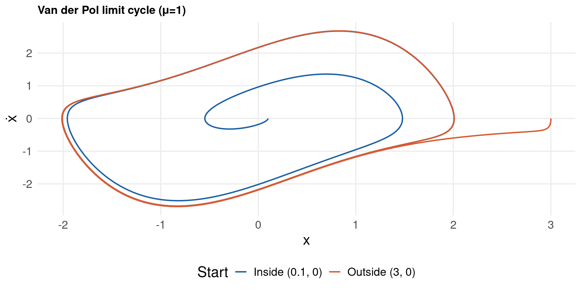
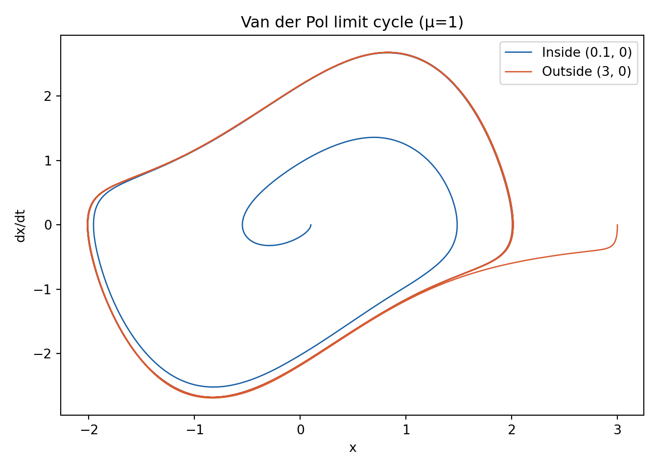
Limit cycle: closed orbit in phase space to which all nearby trajectories converge.

Economic application: endogenous business cycles — persistent oscillations without external shocks.

Energy injection and dissipation: - Near \(|x| < 1\): damping term \(\mu(1-x^2) > 0\) injects energy - For \(|x| > 1\): \(\mu(1-x^2) < 0\) dissipates energy - Net result: stable oscillation of fixed amplitude \(\approx 2\)

For any \(\mu > 0\) and any initial condition (except origin): - Interior trajectories spiral outward to the limit cycle - Exterior trajectories spiral inward to the limit cycle

Phase Plane & Van der Pol

Code
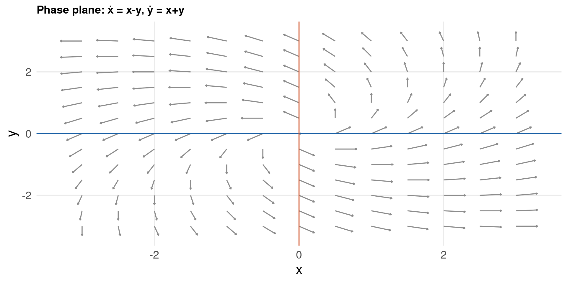
grid <- expand.grid(x = seq(-3, 3, by = 0.5), y = seq(-3, 3, by = 0.5)) %>%
  mutate(
    dx  = x - y,
    dy  = x + y,
    len = sqrt(dx^2 + dy^2) + 1e-6,
    dx  = dx / len * 0.3,
    dy  = dy / len * 0.3
  )

ggplot(grid) +
  aes(x = x, y = y) +
  geom_segment(aes(xend = x + dx, yend = y + dy),
               arrow = arrow(length = unit(0.08, "cm")),
               color = col_muted) +
  geom_hline(yintercept = 0, color = col_main, linewidth = 0.6) +
  geom_vline(xintercept = 0, color = col_accent, linewidth = 0.6) +
  labs(x = "x", y = "y",
       title = "Phase plane: ẋ = x-y (blue), ẏ = x+y (red)") +
  theme_lecture

Code
vdp <- function(t, y, parms) {
  list(c(y[2], parms$mu * (1 - y[1]^2) * y[2] - y[1]))
}
times <- seq(0, 30, by = 0.02)
sol1  <- ode(y = c(x = 0.1, y = 0), times = times,
             func = vdp, parms = list(mu = 1))
sol2  <- ode(y = c(x = 3.0, y = 0), times = times,
             func = vdp, parms = list(mu = 1))

bind_rows(
  as.data.frame(sol1) %>% mutate(ic = "Inside (0.1, 0)"),
  as.data.frame(sol2) %>% mutate(ic = "Outside (3, 0)")
) %>%
  ggplot() +
  aes(x = x, y = y, color = ic) +
  geom_path(linewidth = 0.8) +
  scale_color_manual(values = c(col_main, col_accent), name = "Start") +
  labs(x = "x", y = "ẋ",
       title = "Van der Pol limit cycle (μ=1)") +
  theme_lecture

Code
import numpy as np
import matplotlib.pyplot as plt
from scipy.integrate import solve_ivp

def vdp(t, y, mu):
    return [y[1], mu*(1 - y[0]**2)*y[1] - y[0]]

mu = 1.0
t_span, t_eval = (0, 30), np.linspace(0, 30, 3000)
ics   = [(0.1, 0, "#185FA5", "Inside (0.1, 0)"),
         (3.0, 0, "#D85A30", "Outside (3, 0)")]

fig, ax = plt.subplots(figsize=(7, 5))
for x0, y0, c, lbl in ics:
    sol = solve_ivp(vdp, t_span, [x0, y0], args=(mu,), t_eval=t_eval)
    ax.plot(sol.y[0], sol.y[1], color=c, linewidth=1, label=lbl)
ax.set_xlabel("x"); ax.set_ylabel("dx/dt")
ax.set_title("Van der Pol limit cycle (μ=1)")
ax.legend(); plt.tight_layout(); plt.show()

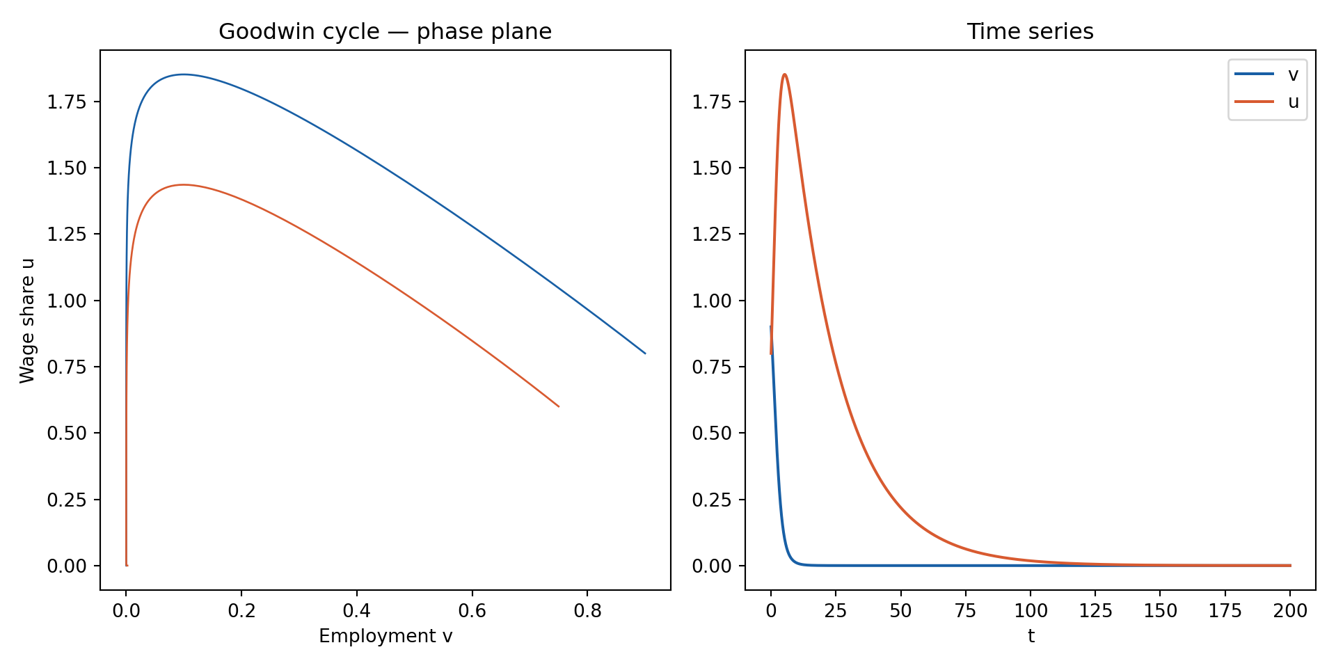
Goodwin Business Cycle Model

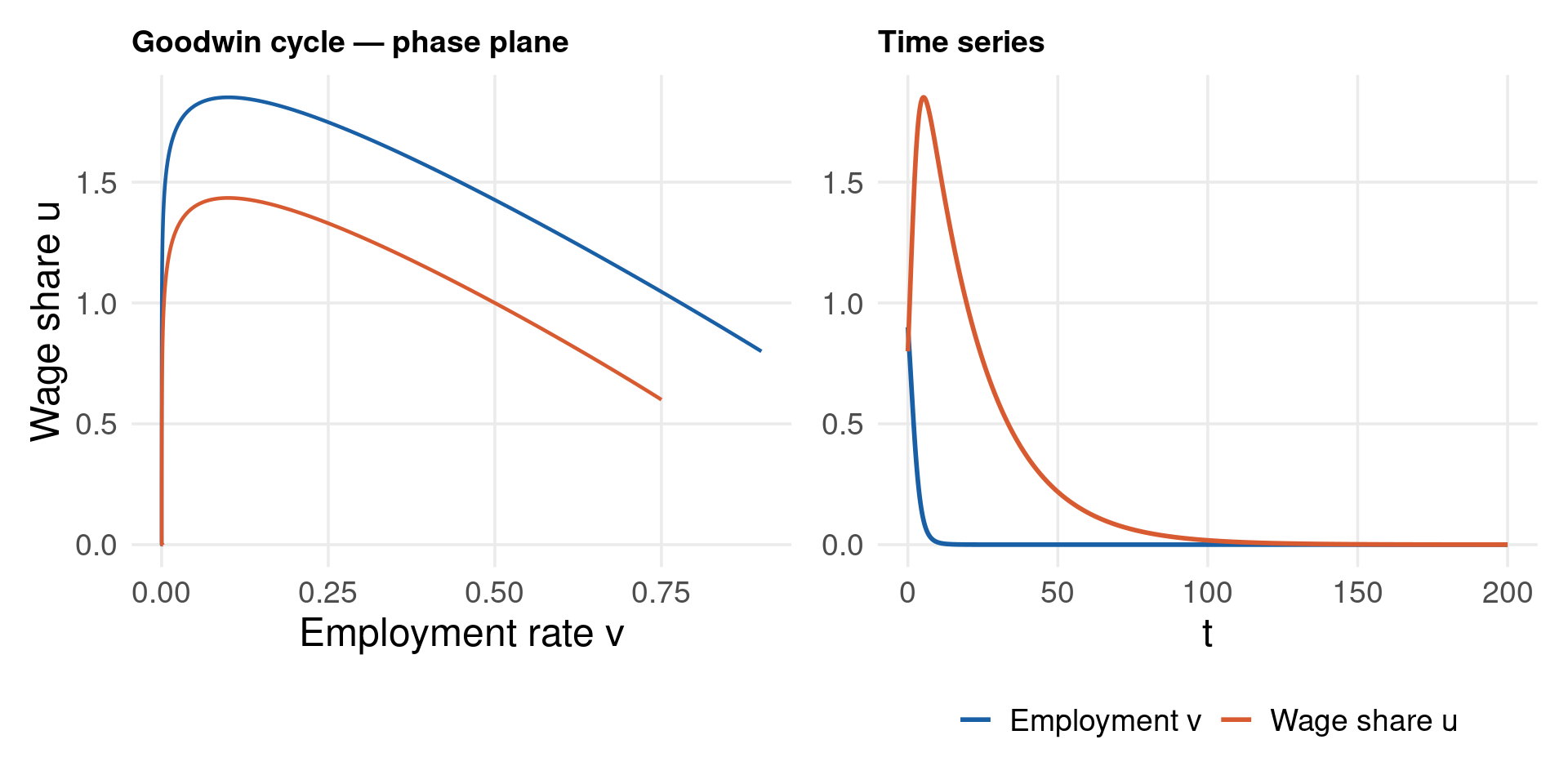
Goodwin (1967) — predator-prey growth cycle:

Let \(u\) = wage share, \(v\) = employment rate:

\[\dot{v} = v(\rho - \alpha u), \qquad \dot{u} = u(\beta v - \gamma)\]

where: - \(\rho\) = labour productivity growth - \(\alpha\) = sensitivity of employment to wage share - \(\beta\) = sensitivity of wage growth to employment - \(\gamma\) = rate of wage adjustment

Fixed point: \(u^* = \rho/\alpha\), \(v^* = \gamma/\beta\)

Trajectories: closed orbits (conservative system, no dissipation) — perpetual cycles.

This reproduces endogenous business cycles with no external shocks — a purely deterministic explanation of fluctuations.

Code
goodwin <- function(t, y, parms) {
  v <- y[1]; u <- y[2]
  list(c(v*(parms$rho - parms$alpha*u),
         u*(parms$beta*v - parms$gamma)))
}
parms_gw <- list(rho=0.03, alpha=0.3, beta=0.5, gamma=0.05)
times_gw  <- seq(0, 200, by = 0.1)
inits_gw  <- list(c(v=0.9, u=0.8), c(v=0.75, u=0.6))
cols_gw   <- c(col_main, col_accent)

traj_gw <- lapply(seq_along(inits_gw), function(i) {
  ode(y = inits_gw[[i]], times = times_gw, func = goodwin, parms = parms_gw) %>%
    as.data.frame() %>%
    mutate(ic = i)
})

p1 <- bind_rows(traj_gw) %>%
  ggplot() +
  aes(x = v, y = u, color = factor(ic)) +
  geom_path(linewidth = 0.8) +
  scale_color_manual(values = cols_gw, guide = "none") +
  labs(x = "Employment rate v", y = "Wage share u",
       title = "Goodwin cycle — phase plane") +
  theme_lecture

p2 <- bind_rows(traj_gw) %>%
  filter(ic == 1) %>%
  ggplot() +
  aes(x = time) +
  geom_line(aes(y = v, color = "Employment v"), linewidth = 1) +
  geom_line(aes(y = u, color = "Wage share u"), linewidth = 1) +
  scale_color_manual(values = c(col_main, col_accent), name = NULL) +
  labs(x = "t", y = NULL, title = "Time series") +
  theme_lecture

p1 + p2

Code
import numpy as np
import matplotlib.pyplot as plt
from scipy.integrate import solve_ivp

def goodwin_rhs(t, y, rho, alpha, beta, gamma):
    v, u = y
    return [v*(rho - alpha*u), u*(beta*v - gamma)]

parms = (0.03, 0.3, 0.5, 0.05)
t_span = (0, 200)
t_eval = np.linspace(0, 200, 2000)
ics = [(0.9, 0.8), (0.75, 0.6)]
colors = ["#185FA5", "#D85A30"]

fig, axes = plt.subplots(1, 2, figsize=(10, 5))
for ic, c in zip(ics, colors):
    sol = solve_ivp(goodwin_rhs, t_span, list(ic), args=parms, t_eval=t_eval)
    axes[0].plot(sol.y[0], sol.y[1], color=c, linewidth=1)
    if c == colors[0]:
        axes[1].plot(sol.t, sol.y[0], color="#185FA5", linewidth=1.5, label="v")
        axes[1].plot(sol.t, sol.y[1], color="#D85A30", linewidth=1.5, label="u")
axes[0].set_xlabel("Employment v"); axes[0].set_ylabel("Wage share u")
axes[0].set_title("Goodwin cycle — phase plane")
axes[1].set_xlabel("t"); axes[1].set_title("Time series")
axes[1].legend()
plt.tight_layout(); plt.show()

Part V: Discrete Systems of Equations

Matrix recursions, eigenvalues, and policy assignment

Linear Discrete Systems

Homogeneous:

\[\mathbf{u}_t = \mathbf{A} \mathbf{u}_{t-1}\]

Non-homogeneous:

\[\mathbf{u}_t = \mathbf{A} \mathbf{u}_{t-1} + \mathbf{b}\]

where \(\mathbf{u}\) is \(n \times 1\), \(\mathbf{A}\) is \(n \times n\), \(\mathbf{b}\) is \(n \times 1\).

2×2 example:

\[x_t = ax_{t-1} + by_{t-1}, \qquad y_t = cx_{t-1} + dy_{t-1}\]

Equilibrium at \(\mathbf{u}^* = \mathbf{A}\mathbf{u}^* + \mathbf{b}\):

\[(\mathbf{I} - \mathbf{A})\mathbf{u}^* = \mathbf{b} \implies \mathbf{u}^* = (\mathbf{I} - \mathbf{A})^{-1}\mathbf{b}\]

provided \((\mathbf{I} - \mathbf{A})\) is non-singular.

Solution by iteration:

\[\mathbf{u}_t = \mathbf{A}^t \mathbf{u}_0\]

Use diagonalisation for efficient computation:

\[\mathbf{u}_t = \mathbf{V}\mathbf{D}^t\mathbf{V}^{-1}\mathbf{u}_0 = ar^t\mathbf{v}^r + bs^t\mathbf{v}^s\]

Eigenvalues & Stability

If \(\mathbf{A}\) has distinct eigenvalues \(r, s\) with eigenvectors \(\mathbf{v}^r, \mathbf{v}^s\), form \(\mathbf{V} = [\mathbf{v}^r \; \mathbf{v}^s]\):

\[\mathbf{D} = \mathbf{V}^{-1}\mathbf{A}\mathbf{V} = \begin{bmatrix} r & 0 \\ 0 & s \end{bmatrix}\]

Solution:

\[\mathbf{u}_t = \mathbf{V}\mathbf{D}^t\mathbf{V}^{-1}\mathbf{u}_0 = ar^t\mathbf{v}^r + bs^t\mathbf{v}^s\]

The system \(\mathbf{u}_t = \mathbf{A}\mathbf{u}_{t-1}\) is asymptotically stable iff:

\[|\lambda_i| < 1 \quad \text{for all eigenvalues}\]

Unit circle criterion: eigenvalues must lie strictly inside the unit circle in the complex plane.

Jordan forms:

Eigenvalues Jordan \(\mathbf{J}\)
Real distinct \(r, s\) \(\text{diag}(r, s)\)
Repeated \(\lambda\) \(\begin{bmatrix}\lambda & 1 \\ 0 & \lambda\end{bmatrix}\)
Complex \(\alpha \pm \beta i\) \(|\alpha + \beta i|^2 = \alpha^2+\beta^2 < 1\)

Trajectories — 2×2 Discrete System

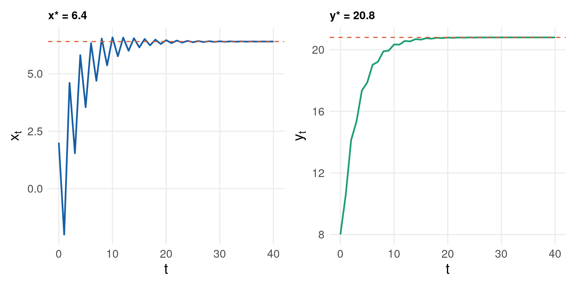
\[x_{t+1} = -8 - x_t + y_t, \qquad y_{t+1} = 4 - 0.3x_t + 0.9y_t\]

Matrix \(\mathbf{A} = \begin{bmatrix}-1 & 1 \\ -0.3 & 0.9\end{bmatrix}\), \(\mathbf{b} = \begin{bmatrix}-8\\4\end{bmatrix}\)

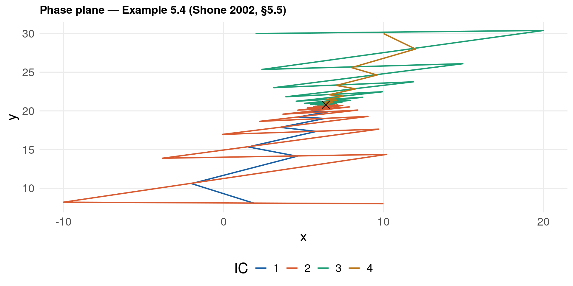
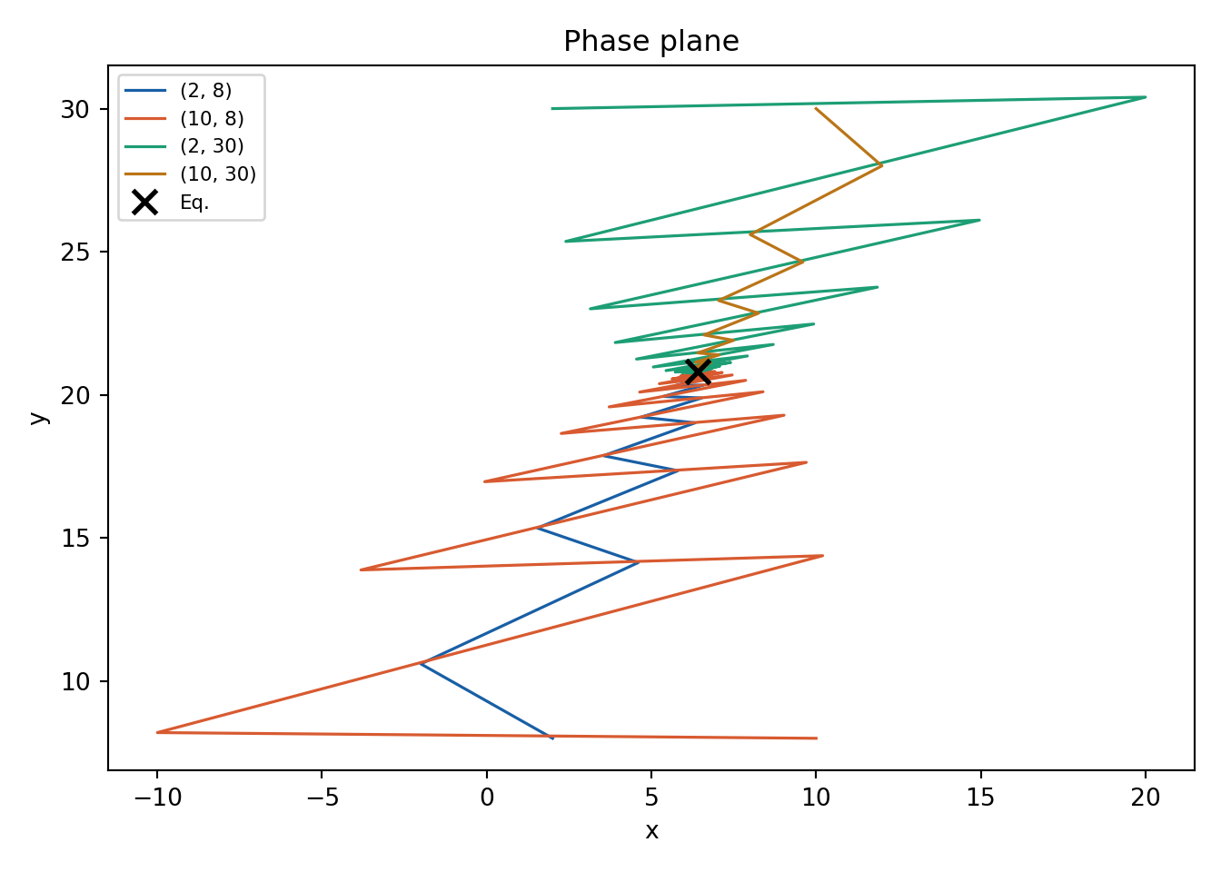
Fixed point: \((x^*, y^*) = (6.4, \; 20.8)\)

Characteristic equation: \(\lambda^2 + 0.1\lambda - 0.6 = 0\)

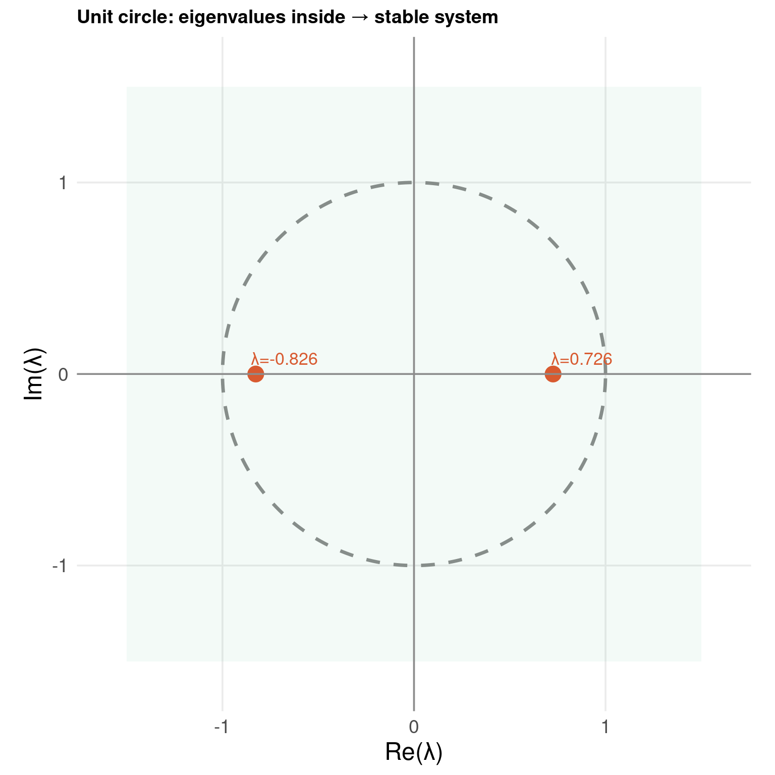
Eigenvalues: \(r = 0.7262\), \(s = -0.8262\)

\[|r| = 0.726 < 1, \quad |s| = 0.826 < 1\]

Both inside unit circle → asymptotically stable.

Negative \(s\) → oscillations (sign alternation) while converging.

Eigenvectors:

For \(r = 0.7262\): \(\mathbf{v}^r = \begin{bmatrix}0.5793\\1\end{bmatrix}\)

For \(s = -0.8262\): \(\mathbf{v}^s = \begin{bmatrix}5.7537\\1\end{bmatrix}\)

Internal & External Balance

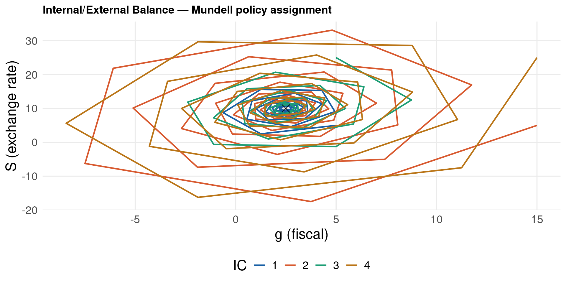
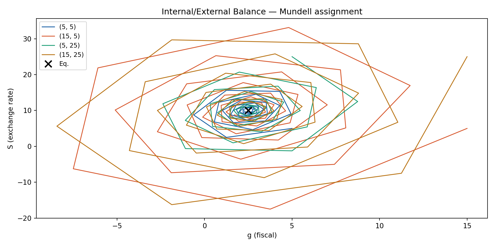
Two targets, two instruments: - \(g_t\): government expenditure (fiscal policy) - \(S_t\): exchange rate (monetary policy) - Internal balance: \(g^*_t = -2.5 + 0.5 S_t\) - External balance: \(S^*_t = 20 - 4 g_t\)

Adjustment dynamics:

\[\Delta g_{t+1} = -0.75(g_t - g^*_t), \qquad \Delta S_{t+1} = -0.5(S_t - S^*_t)\]

\[\begin{bmatrix}g_{t+1}\\S_{t+1}\end{bmatrix} = \begin{bmatrix}0.25 & 0.375\\-2 & 0.5\end{bmatrix}\begin{bmatrix}g_t\\S_t\end{bmatrix} + \begin{bmatrix}-1.875\\10\end{bmatrix}\]

Stability check: eigenvalues of \(\mathbf{A}\) must satisfy \(|\lambda_i| < 1\).

Discrete Systems Code

Code
A_mat  <- matrix(c(-1, -0.3, 1, 0.9), nrow = 2)
b_vec  <- c(-8, 4)
u_star <- solve(diag(2) - A_mat) %*% b_vec

T  <- 40
xy <- matrix(0, nrow = T + 1, ncol = 2); xy[1, ] <- c(2, 8)
for (t in seq_len(T)) xy[t+1, ] <- A_mat %*% xy[t, ] + b_vec

df <- data.frame(t = 0:T, x = xy[, 1], y = xy[, 2])

p1 <- ggplot(df) +
  aes(x = t, y = x) +
  geom_line(color = col_main, linewidth = 1) +
  geom_hline(yintercept = u_star[1], linetype = "dashed", color = col_accent) +
  labs(x = "t", y = expression(x[t]),
       title = glue("x* = {round(u_star[1],1)}")) +
  theme_lecture

p2 <- ggplot(df) +
  aes(x = t, y = y) +
  geom_line(color = col_ok, linewidth = 1) +
  geom_hline(yintercept = u_star[2], linetype = "dashed", color = col_accent) +
  labs(x = "t", y = expression(y[t]),
       title = glue("y* = {round(u_star[2],1)}")) +
  theme_lecture

p1 + p2

Code
ics_v  <- list(c(2, 8), c(10, 8), c(2, 30), c(10, 30))
cols_v <- c(col_main, col_accent, col_ok, col_warn)
T3 <- 60

traj_list <- lapply(seq_along(ics_v), function(i) {
  xy3 <- matrix(0, nrow = T3 + 1, ncol = 2); xy3[1, ] <- ics_v[[i]]
  for (t in seq_len(T3)) xy3[t+1, ] <- A_mat %*% xy3[t, ] + b_vec
  data.frame(x = xy3[, 1], y = xy3[, 2], ic = i)
})

bind_rows(traj_list) %>%
  ggplot() +
  aes(x = x, y = y, color = factor(ic)) +
  geom_path(linewidth = 0.8) +
  geom_point(data = data.frame(x = u_star[1], y = u_star[2]),
             aes(x = x, y = y), inherit.aes = FALSE,
             size = 4, color = "black", shape = 4) +
  scale_color_manual(values = cols_v, name = "IC") +
  labs(x = "x", y = "y",
       title = "Phase plane — Example 5.4 (Shone 2002, §5.5)") +
  theme_lecture

Code
import numpy as np
import matplotlib.pyplot as plt

A_m   = np.array([[-1, 1], [-0.3, 0.9]])
b_v   = np.array([-8.0, 4.0])
u_eq  = np.linalg.solve(np.eye(2) - A_m, b_v)

ics_p  = [(2, 8), (10, 8), (2, 30), (10, 30)]
cols_p = ["#185FA5", "#D85A30", "#1D9E75", "#BA7517"]
T_p    = 60

fig, ax = plt.subplots(figsize=(7, 5))
for ic, c in zip(ics_p, cols_p):
    xy = np.zeros((T_p + 1, 2)); xy[0] = ic
    for t in range(T_p): xy[t+1] = A_m @ xy[t] + b_v
    ax.plot(xy[:, 0], xy[:, 1], color=c, linewidth=1.2, label=str(ic))
ax.plot(*u_eq, "kx", markersize=10, markeredgewidth=2, label="Eq.")
ax.set_xlabel("x"); ax.set_ylabel("y")
ax.set_title("Phase plane")
ax.legend(fontsize=8); plt.tight_layout(); plt.show()

Discrete System Code — Eigenvalue Stability

Code
theta   <- seq(0, 2*pi, length.out = 300)
circle  <- data.frame(x = cos(theta), y = sin(theta))

A_eig   <- matrix(c(-1, -0.3, 1, 0.9), nrow = 2)
evals   <- eigen(A_eig)$values
ev_df   <- data.frame(
  Re  = Re(evals), Im = Im(evals),
  lbl = paste0("λ", seq_along(evals), "=", round(evals, 3))
)

ggplot() +
  geom_path(data = circle, aes(x = x, y = y),
            color = col_muted, linewidth = 1.2, linetype = "dashed") +
  geom_point(data = ev_df, aes(x = Re, y = Im), color = col_accent, size = 4) +
  geom_text(data = ev_df,
    aes(x = Re + 0.12, y = Im + 0.1, label = lbl),
    size = 4, color = col_accent, hjust = 0) +
  geom_hline(yintercept = 0, color = col_muted) +
  geom_vline(xintercept = 0, color = col_muted) +
  coord_fixed() +
  labs(x = "Re(λ)", y = "Im(λ)", title = "Eigenvalues in complex plane — inside unit circle → stable") +
  theme_lecture

Code
A_bal  <- matrix(c(0.25, -2, 0.375, 0.5), nrow = 2)
b_bal  <- c(-1.875, 10)
u_bal  <- solve(diag(2) - A_bal) %*% b_bal

ics_b  <- list(c(5, 5), c(15, 5), c(5, 25), c(15, 25))
T_bal  <- 40
cols_b <- c(col_main, col_accent, col_ok, col_warn)

traj_b <- lapply(seq_along(ics_b), function(i) {
  xy <- matrix(0, T_bal+1, 2); xy[1,] <- ics_b[[i]]
  for (t in seq_len(T_bal)) xy[t+1,] <- A_bal %*% xy[t,] + b_bal
  data.frame(g = xy[,1], S = xy[,2], ic = i)
})

bind_rows(traj_b) %>%
  ggplot() +
  aes(x = g, y = S, color = factor(ic)) +
  geom_path(linewidth = 0.9) +
  geom_point(data = data.frame(g = u_bal[1], S = u_bal[2]),
             aes(x = g, y = S), inherit.aes = FALSE,
             color = "black", size = 4, shape = 4) +
  scale_color_manual(values = cols_b, name = "IC") +
  labs(x = "g (fiscal)", y = "S (exchange rate)",
       title = "Internal/External Balance — Mundell policy assignment") +
  theme_lecture

Code
import numpy as np
import matplotlib.pyplot as plt

A = np.array([[0.25, 0.375], [-2.0, 0.5]])
b = np.array([-1.875, 10.0])
eq = np.linalg.solve(np.eye(2) - A, b)

ics = [(5,5), (15,5), (5,25), (15,25)]
colors = ["#185FA5", "#D85A30", "#1D9E75", "#BA7517"]
T = 40

fig, ax = plt.subplots(figsize=(10, 5))
for ic, c in zip(ics, colors):
    xy = np.zeros((T+1, 2)); xy[0] = ic
    for t in range(T): xy[t+1] = A @ xy[t] + b
    ax.plot(xy[:,0], xy[:,1], color=c, linewidth=1.2, label=str(ic))
ax.plot(*eq, "kx", markersize=10, markeredgewidth=2, label="Eq.")
ax.set_xlabel("g (fiscal)"); ax.set_ylabel("S (exchange rate)")
ax.set_title("Internal/External Balance — Mundell assignment")
ax.legend(fontsize=9); plt.tight_layout(); plt.show()

Part VI: Optimal Control Theory

Pontryagin principle, Hamiltonians, and dynamic optimisation

The Optimal Control Problem

  • \(x(t)\): state variable — describes the system
  • \(u(t)\): control variable — the policy instrument
  • \(J\): objective function — maximise/minimise
  • \(\dot{x} = f(x, u)\): equation of motion

Continuous formulation:

\[\max_{\{u(t)\}} J = \int_0^T V(x, u) \, dt, \qquad \text{s.t.} \quad \dot{x} = f(x, u), \quad x(0) = x^0, \quad x(T) = x^T\]

Three approaches: (1) calculus of variations, (2) dynamic programming, (3) Pontryagin maximum principle.

\[\max_{\{u_t\}} J = \sum_{t=0}^{T-1} V(\mathbf{x}_t, \mathbf{u}_t, t) + F(\mathbf{x}^T, T), \qquad \mathbf{x}_{t+1} - \mathbf{x}_t = f(\mathbf{x}_t, \mathbf{u}_t, t)\]

Pontryagin Maximum Principle — Continuous

Hamiltonian function:

\[H(x, u) = V(x, u) + \lambda f(x, u)\]

\(\lambda(t)\): costate variable (shadow price of \(\dot{x} = f\)).

First-order conditions:

\[\text{(i)}\ \frac{\partial H}{\partial u} = 0, \quad \text{(ii)}\ \dot{\lambda} = -\frac{\partial H}{\partial x}, \quad \text{(iii)}\ \dot{x} = \frac{\partial H}{\partial \lambda} = f(x,u)\]

\[\text{(iv)}\ x(0) = x^0, \quad \text{(v)}\ \lambda(T) = 0 \quad \text{(transversality)}\]

  1. Specify \(H = V + \lambda f\); apply condition (i)
  2. Solve \(\partial H/\partial u = 0\) for \(u = h(\lambda)\)
  3. Substitute \(u^*\) back: obtain two ODEs in \(x\) and \(\lambda\)
  4. Solve for general solutions with constants \(c_1, c_2\)
  5. Apply boundary conditions \(x(0) = x^0\), \(\lambda(T) = 0\) to pin \(c_1, c_2\)
  6. Substitute \(\lambda^*(t)\) to obtain \(u^*(t)\)

Pontryagin: Discrete & Discounting

Discrete Hamiltonian:

\[H(x_t, u_t) = V(x_t, u_t) + \lambda_{t+1} f(x_t, u_t)\]

Costate is forward-dated \(\lambda_{t+1}\).

Conditions:

\[\frac{\partial H}{\partial u_t} = 0, \quad t = 0,\ldots,T-1\]

\[\lambda_{t+1} - \lambda_t = -\frac{\partial H}{\partial x_t}, \quad t = 1,\ldots,T-1\]

\[x_{t+1} - x_t = f(x_t, u_t), \quad \lambda_T = 0, \quad x_0 = a\]

Solve backwards from \(\lambda_T = 0\).

Continuous:

\[\max J = \int_0^T e^{-\delta t} V(x, u) \, dt\]

Current value Hamiltonian: \(H_c = V + \mu f\), where \(\mu = \lambda e^{\delta t}\).

Modified costate: \(\dot{\mu} = -\partial H_c/\partial x + \delta\mu\)

Discrete:

\[\max J = \sum_{t=0}^{T-1} \rho^t V(x_t, u_t), \quad \rho = \frac{1}{1+\delta}\]

Current value Hamiltonian: \(H_c = V + \rho\lambda_{t+1}f\)

Phase Diagram for Optimal Control

After substituting \(u^* = u(x, \lambda)\) from condition (i), the system becomes autonomous in \((x, \lambda)\):

\[\dot{x} = F(x, \lambda), \qquad \dot{\lambda} = G(x, \lambda)\]

Nullclines: - \(\dot{x} = 0\): \(\lambda\) as function of \(x\) when \(x\) stationary - \(\dot{\lambda} = 0\): analogously

Intersection = steady state \((x^{ss}, \lambda^{ss})\).

Optimal control problems typically yield a saddle point in the \((x, \lambda)\) phase plane: - One stable manifold: the saddle path - One unstable manifold

The transversality condition \(\lambda(\infty) = 0\) selects the unique trajectory on the saddle path.

Optimal Control Code

Code
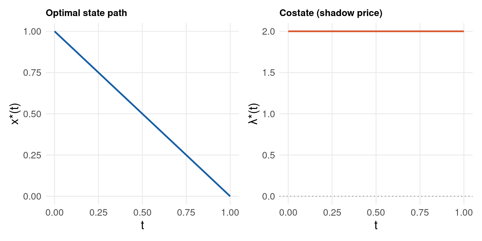
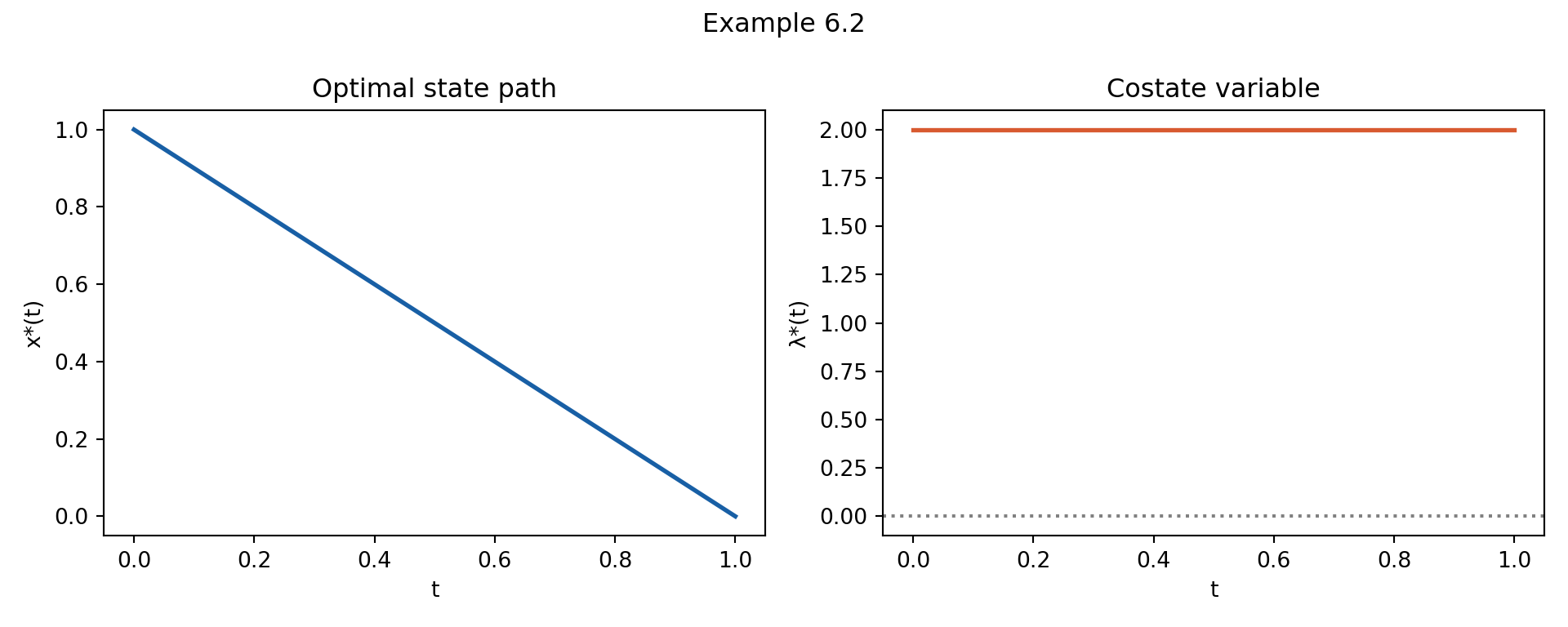
# Example 6.2: max ∫₀¹ u² dt, ẋ = -u, x(0)=1, x(1)=0
# Solution: x*(t) = 1-t, u*(t) = 1, λ*(t) = 2
t_v <- seq(0, 1, by = 0.01)

df_oc <- data.frame(
  t        = t_v,
  x_star   = 1 - t_v,
  u_star   = rep(1, length(t_v)),
  lam_star = rep(2, length(t_v))
)

p1 <- ggplot(df_oc) +
  aes(x = t, y = x_star) +
  geom_line(color = col_main, linewidth = 1.2) +
  labs(x = "t", y = "x*(t)", title = "Optimal state path") +
  theme_lecture

p2 <- ggplot(df_oc) +
  aes(x = t, y = lam_star) +
  geom_line(color = col_accent, linewidth = 1.2) +
  geom_hline(yintercept = 0, linetype = "dotted", color = col_muted) +
  labs(x = "t", y = "λ*(t)", title = "Costate (shadow price)") +
  theme_lecture

p1 + p2

Code
# Example 6.3: ẋ = x+2λ, λ̇ = x/2 - λ
# Eigenvalues: ±√2 → saddle point
saddle_sys <- function(t, y, parms) {
  list(c(y[1] + 2*y[2], 0.5*y[1] - y[2]))
}

# Stable arm: initial conditions near saddle (0,0) on stable eigenvector
eig_stable <- -sqrt(2)   # stable eigenvalue
v_stable   <- c(y1 = 2, y2 = eig_stable - 1)

eps <- 0.3
starts <- list(eps * v_stable, -eps * v_stable)
times  <- seq(0, 3, by = 0.01)

traj <- lapply(starts, function(y0) {
  sol <- ode(y = y0, times = times, func = saddle_sys, parms = list())
  as.data.frame(sol) %>% mutate(arm = "stable")
})

do.call(rbind, traj) %>%
  ggplot() +
  aes(x = y1, y = y2, color = arm) +
  geom_path(linewidth = 1.2, color = col_main) +
  geom_point(aes(x = 0, y = 0), color = "black", size = 3, shape = 4,
             inherit.aes = FALSE) +
  labs(x = "x", y = "λ",
       title = "Saddle path — Example 6.3 (Shone 2002, §6.5)") +
  theme_lecture

Code
import numpy as np
import matplotlib.pyplot as plt

# Example 6.2: x*(t) = 1-t, u*(t) = 1, λ*(t) = 2
t = np.linspace(0, 1, 100)

fig, axes = plt.subplots(1, 2, figsize=(10, 4))
axes[0].plot(t, 1 - t, color="#185FA5", linewidth=2)
axes[0].set_xlabel("t"); axes[0].set_ylabel("x*(t)")
axes[0].set_title("Optimal state path")

axes[1].plot(t, np.full_like(t, 2.0), color="#D85A30", linewidth=2)
axes[1].axhline(0, linestyle=":", color="grey")
axes[1].set_xlabel("t"); axes[1].set_ylabel("λ*(t)")
axes[1].set_title("Costate variable")

plt.suptitle("Example 6.2")
plt.tight_layout(); plt.show()

Ramsey-Cass-Koopmans Model

Social planner maximises discounted utility:

\[\max_{\{c(t)\}} \int_0^\infty e^{-\rho t} u(c) \, dt, \quad u(c) = \frac{c^{1-\sigma}-1}{1-\sigma}\]

Subject to capital accumulation:

\[\dot{k} = f(k) - c - \delta k, \quad f(k) = Ak^\alpha\]

Current value Hamiltonian: \(H_c = u(c) + \mu[f(k) - c - \delta k]\)

First-order conditions:

\[\frac{\partial H_c}{\partial c} = 0 \implies u'(c) = \mu \implies \mu = c^{-\sigma}\]

\[\dot{\mu} = (\rho + \delta)\mu - \mu f'(k) \implies \frac{\dot{c}}{c} = \frac{f'(k) - \delta - \rho}{\sigma}\]

Ramsey-Euler equation (consumption Euler equation):

\[\frac{\dot{c}}{c} = \frac{r(k) - \rho}{\sigma}, \quad r(k) = f'(k) - \delta = \alpha A k^{\alpha-1} - \delta\]

Saddle path: The \((k, c)\) phase plane has a saddle equilibrium. The unique optimal trajectory is the saddle path — the economy jumps to it at \(t=0\) given \(k_0\), then follows it to \((k^*, c^*)\).

Iron ore mine — exhaustible resource:

\[\max \sum_{t=0}^{T-1} \rho^t p \cdot u_t, \qquad x_{t+1} = x_t - u_t, \quad u_t \geq 0, \quad x_T \geq 0\]

Discrete Hamiltonian: \(H_t = \rho^t p \cdot u_t + \lambda_{t+1}(x_t - u_t)\)

FOC: \(\rho^t p = \lambda_{t+1}\) — at optimum, \(\lambda_{t+1}\) grows at rate \(1/\rho = 1+\delta\) per period.

Hotelling rule: \(\lambda_{t+1}/\lambda_t = 1+\delta\) — the royalty (scarcity rent) rises at the interest rate.

Discrete Mine Problem — Code

Code
p_price <- 10; delta <- 0.1; rho <- 1/(1+delta)
T_mine  <- 10; x0_mine <- 100

# Hotelling: u_t = u_0 * (rho)^t, sum(u_t) = x0
# u_0 * sum(rho^t, t=0..T-1) = x0
u0 <- x0_mine / sum(rho^(0:(T_mine-1)))
u_opt  <- u0 * rho^(0:(T_mine-1))
x_opt  <- x0_mine - cumsum(c(0, u_opt))

df_mine <- data.frame(
  t = 0:(T_mine-1),
  u = u_opt,
  x = x_opt[1:T_mine],
  lambda = p_price * rho^(-(0:(T_mine-1)))
)

p1 <- ggplot(df_mine) +
  aes(x = t, y = u) +
  geom_col(fill = col_main, width = 0.6) +
  labs(x = "t", y = "Extraction u(t)", title = "Optimal extraction path") +
  theme_lecture

p2 <- ggplot(df_mine) +
  aes(x = t, y = lambda) +
  geom_line(color = col_accent, linewidth = 1.3) +
  geom_point(color = col_accent, size = 3) +
  labs(x = "t", y = "λ(t) — royalty", title = "Hotelling royalty (rises at rate δ)") +
  theme_lecture

p1 + p2

Code
import numpy as np
import matplotlib.pyplot as plt

p, delta = 10, 0.1
rho = 1 / (1 + delta)
T, x0 = 10, 100

u0 = x0 / sum(rho**t for t in range(T))
u_opt = np.array([u0 * rho**t for t in range(T)])
royalty = np.array([p * rho**(-t) for t in range(T)])

fig, axes = plt.subplots(1, 2, figsize=(10, 5))
axes[0].bar(range(T), u_opt, color="#185FA5", width=0.6)
axes[0].set_xlabel("t"); axes[0].set_ylabel("u(t)")
axes[0].set_title("Optimal extraction path")

axes[1].plot(range(T), royalty, color="#D85A30", linewidth=2, marker="o")
axes[1].set_xlabel("t"); axes[1].set_ylabel("λ(t)")
axes[1].set_title("Hotelling royalty (rises at rate δ)")
plt.tight_layout(); plt.show()

Part VII: Chaos Theory

Bifurcations, strange attractors, and limits of prediction

Bifurcations

A bifurcation occurs when a small smooth change in a parameter causes a sudden qualitative change in system behaviour.

Types relevant to economics: - Pitchfork: one fixed point splits into two stable ones - Transcritical: fixed points exchange stability - Hopf: equilibrium loses stability; limit cycle born (see Part IV) - Period-doubling: period-\(n\) cycle → period-\(2n\) — route to chaos

\[x_t = \lambda x_{t-1}(1-x_{t-1})\]

\(\lambda\) Attractor
\(1 < \lambda \leq 3\) fixed point \(x^* = 1-1/\lambda\)
\(\lambda \approx 3\) 1st bifurcation → period-2
\(\lambda \approx 3.449\) 2nd → period-4
\(\lambda \approx 3.544\) 3rd → period-8
\(\lambda \approx 3.569\) onset of chaos
\(\lambda > 3.57\) chaos (with periodic windows)

Feigenbaum Constant & Sarkovskii

Bifurcation points \(\lambda_n\) converge geometrically:

\[\delta_F = \lim_{n\to\infty} \frac{\lambda_n - \lambda_{n-1}}{\lambda_{n+1} - \lambda_n} \approx 4.6692\ldots\]

Universal: appears in all period-doubling cascades, not just the logistic map.

Accumulation point: \(\lambda_\infty \approx 3.5699\ldots\) (onset of chaos).

From \(\lambda_1 \approx 3.000\), \(\lambda_2 \approx 3.449\), \(\lambda_3 \approx 3.544\):

\[\hat\delta_F \approx \frac{3.449 - 3.000}{3.544 - 3.449} = \frac{0.449}{0.095} \approx 4.73\]

Order the positive integers:

\[3 \triangleright 5 \triangleright 7 \triangleright \cdots \triangleright 2\cdot3 \triangleright 2\cdot5 \triangleright \cdots \triangleright 2^2 \triangleright 2 \triangleright 1\]

If \(f\) has a periodic orbit of period \(m\) and \(m \triangleright n\), then \(f\) also has a periodic orbit of period \(n\).

Corollary: If \(f\) has a period-3 orbit, it has orbits of every period.

“Period 3 implies chaos” — Li & Yorke (1975), doi:10.2307/2318254.

Hopf Bifurcation & Van der Pol

As parameter \(\mu\) crosses critical value \(\mu_c\): - \(\mu < \mu_c\): stable spiral (all trajectories → equilibrium) - \(\mu = \mu_c\): purely imaginary eigenvalues \(\pm\beta i\)centre - \(\mu > \mu_c\): equilibrium unstable; limit cycle born continuously

The equilibrium loses stability and a closed orbit emerges — this is the supercritical Hopf bifurcation.

\[\dot{x} = y, \quad \dot{y} = \mu(1-x^2)y - x\]

  • At \(\mu = 0\): centre (neutral stability, no dissipation)
  • For \(\mu > 0\): limit cycle of amplitude \(\approx 2\) emerges
  • As \(\mu \to \infty\): relaxation oscillations — slow drift punctuated by fast jumps (slow-fast dynamics)

Lorenz Strange Attractor

\[\dot{x} = \sigma(y - x), \qquad \dot{y} = \rho x - y - xz, \qquad \dot{z} = xy - \beta z\]

Standard parameters: \(\sigma=10\), \(\rho=28\), \(\beta=8/3\)

Properties: - Strange attractor: bounded, non-repeating trajectories - Sensitive dependence: “butterfly effect” — nearby paths diverge exponentially - Positive Lyapunov exponent: \(\lambda_1 \approx 0.906\)

Originally atmospheric convection (Lorenz, 1963). Demonstrates: deterministic systems can be fundamentally unpredictable.

Implications for economics: - Fundamental limits on forecasting exchange rates, financial prices, business cycles - Positive Lyapunov exponent → forecasting horizon \(\approx 1/\lambda_1\) - Related phenomena: sunspot equilibria, exchange rate chaos

Phase space structure:

Two “wings” — trajectories circle one wing for a while, then switch unpredictably. The number of loops per wing is irregular and never exactly repeats.

Chaos Code

Code
logistic_orbit <- function(lam, n_burn = 500, n_keep = 300) {
  x <- 0.5
  for (i in seq_len(n_burn)) x <- lam * x * (1 - x)
  xs <- numeric(n_keep)
  for (i in seq_len(n_keep)) { x <- lam * x * (1 - x); xs[i] <- x }
  data.frame(lambda = lam, x = xs)
}

bif <- do.call(rbind, lapply(seq(2.5, 4.0, by = 0.004), logistic_orbit))

ggplot(bif) +
  aes(x = lambda, y = x) +
  geom_point(size = 0.05, color = col_main, alpha = 0.4) +
  labs(x = expression(lambda), y = expression(x[t]),
       title = "Bifurcation diagram — logistic map (Shone 2002, §7.3)") +
  theme_lecture

Code
lorenz <- function(t, y, parms) {
  with(as.list(c(y, parms)), {
    list(c(sigma * (Y - X), rho * X - Y - X * Z, X * Y - beta * Z))
  })
}
parms_lz <- c(sigma = 10, rho = 28, beta = 8/3)
sol_lz   <- ode(y = c(X = 1, Y = 1, Z = 1),
                times = seq(0, 50, by = 0.01),
                func = lorenz, parms = parms_lz)

as.data.frame(sol_lz) %>%
  filter(time > 5) %>%
  ggplot() +
  aes(x = X, y = Z) +
  geom_path(color = col_main, linewidth = 0.3, alpha = 0.7) +
  labs(x = "x(t)", y = "z(t)",
       title = "Lorenz strange attractor (σ=10, ρ=28, β=8/3)") +
  theme_lecture

Code
import numpy as np
import matplotlib.pyplot as plt

lam_vals = np.linspace(2.5, 4.0, 1500)
n_burn, n_keep = 500, 300
xs_b, ls_b = [], []

for lam in lam_vals:
    x = 0.5
    for _ in range(n_burn): x = lam * x * (1 - x)
    for _ in range(n_keep):
        x = lam * x * (1 - x)
        xs_b.append(x); ls_b.append(lam)

fig, ax = plt.subplots(figsize=(9, 4))
ax.scatter(ls_b, xs_b, s=0.02, color="#185FA5", alpha=0.4)
<matplotlib.collections.PathCollection object at 0x75e11c32e5c0>
Code
ax.set_xlabel("λ"); ax.set_ylabel("x")
Text(0.5, 0, 'λ')
Text(0, 0.5, 'x')
Code
ax.set_title("Bifurcation diagram — logistic map (Shone 2002, §7.3)")
Text(0.5, 1.0, 'Bifurcation diagram — logistic map (Shone 2002, §7.3)')
Code
plt.tight_layout(); plt.show()

Code
import numpy as np
import matplotlib.pyplot as plt
from scipy.integrate import solve_ivp

def lorenz_rhs(t, y, sigma, rho, beta):
    x, yy, z = y
    return [sigma*(yy - x), rho*x - yy - x*z, x*yy - beta*z]

sol_lz = solve_ivp(lorenz_rhs, [0, 50], [1, 1, 1],
                   args=(10, 28, 8/3), max_step=0.01,
                   t_eval=np.linspace(0, 50, 5000))
mask = sol_lz.t > 5

fig, ax = plt.subplots(figsize=(8, 5))
ax.plot(sol_lz.y[0][mask], sol_lz.y[2][mask],
        color="#185FA5", linewidth=0.3, alpha=0.7)
[<matplotlib.lines.Line2D object at 0x75e11c3d00d0>]
Code
ax.set_xlabel("x(t)"); ax.set_ylabel("z(t)")
Text(0.5, 0, 'x(t)')
Text(0, 0.5, 'z(t)')
Code
ax.set_title("Lorenz strange attractor")
Text(0.5, 1.0, 'Lorenz strange attractor')
Code
plt.tight_layout(); plt.show()

Sensitivity to Initial Conditions

Sensitivity to initial conditions (SIC) is the hallmark of chaos:

\[|x_t(\epsilon) - x_t(0)| \sim |\epsilon| \, e^{\lambda_1 t}\]

where \(\lambda_1 > 0\) is the maximal Lyapunov exponent.

Prediction horizon: errors grow until they are \(O(1)\) — the “doubling time” is \(\tau \approx \ln(2)/\lambda_1\).

Code
lam_sic <- 3.9; T_sic <- 50
x1 <- numeric(T_sic + 1); x1[1] <- 0.5
x2 <- numeric(T_sic + 1); x2[1] <- 0.5 + 1e-6   # tiny perturbation
for (t in seq_len(T_sic)) {
  x1[t+1] <- lam_sic * x1[t] * (1 - x1[t])
  x2[t+1] <- lam_sic * x2[t] * (1 - x2[t])
}
data.frame(t = 0:T_sic, x1 = x1, x2 = x2, diff = abs(x1 - x2)) %>%
  ggplot() +
  aes(x = t) +
  geom_line(aes(y = x1), color = col_main, linewidth = 0.8, alpha = 0.8) +
  geom_line(aes(y = x2), color = col_accent, linewidth = 0.8, linetype = "dashed") +
  labs(x = "t", y = "x(t)",
       title = glue("Logistic map λ={lam_sic}: two trajectories, |Δx(0)|=1e-6")) +
  theme_lecture

Code
lyapunov <- function(lam, n = 1000) {
  x <- 0.5
  for (i in 1:100) x <- lam * x * (1-x)   # burn-in
  le <- 0
  for (i in 1:n) {
    le <- le + log(abs(lam * (1 - 2*x)))
    x <- lam * x * (1-x)
  }
  le / n
}

lam_v  <- seq(2.5, 4.0, by = 0.005)
le_v   <- sapply(lam_v, lyapunov)
df_le  <- data.frame(lambda = lam_v, LE = le_v)

ggplot(df_le) +
  aes(x = lambda, y = LE) +
  geom_line(color = col_main, linewidth = 0.7) +
  geom_hline(yintercept = 0, linetype = "dashed", color = col_accent, linewidth = 0.9) +
  annotate("text", x = 3.65, y = 0.05, label = "LE = 0 (bifurcation points)",
           color = col_accent, size = 4) +
  labs(x = expression(lambda), y = "Lyapunov exponent",
       title = "Lyapunov exponent: positive → chaos, zero → bifurcation") +
  theme_lecture

Code
import numpy as np
import matplotlib.pyplot as plt

def lyapunov(lam, n=1000):
    x = 0.5
    for _ in range(100): x = lam * x * (1-x)
    le = sum(np.log(abs(lam*(1-2*x))) for _ in range(n)
             if (setattr(lyapunov, '_x', x) or True)
             ) / n
    return le

lam_vals = np.linspace(2.5, 4.0, 300)
les = []
for lam in lam_vals:
    x = 0.5
    for _ in range(100): x = lam * x * (1-x)
    le = 0
    for _ in range(1000):
        le += np.log(abs(lam * (1 - 2*x)))
        x = lam * x * (1-x)
    les.append(le / 1000)

fig, ax = plt.subplots(figsize=(10, 5))
ax.plot(lam_vals, les, color="#185FA5", linewidth=0.8)
[<matplotlib.lines.Line2D object at 0x75e119a9d9f0>]
Code
ax.axhline(0, linestyle="--", color="#D85A30", linewidth=1)
<matplotlib.lines.Line2D object at 0x75e119a9e0e0>
Code
ax.set_xlabel("λ", fontsize=13); ax.set_ylabel("Lyapunov exponent", fontsize=13)
Text(0.5, 0, 'λ')
Text(0, 0.5, 'Lyapunov exponent')
Code
ax.set_title("Lyapunov exponent: positive → chaos, zero → bifurcation", fontsize=14)
Text(0.5, 1.0, 'Lyapunov exponent: positive → chaos, zero → bifurcation')
Code
plt.tight_layout(); plt.show()

Economic Implications of Chaos

If economic dynamics are chaotic: - Short-run forecasts remain feasible (within \(1/\lambda_1\) periods) - Long-run forecasts are fundamentally unreliable — not just statistically uncertain, but physically impossible given finite measurement precision - Observed volatility in financial markets may be deterministic chaos, not random noise

Tests for chaos in economic time series:

Method What it measures
BDS test i.i.d. against nonlinear dependence
Correlation dimension fractal dimension of attractor
Lyapunov exponent divergence rate of nearby trajectories
Recurrence plots structure of the phase portrait

Empirical findings: Some evidence of nonlinearity in exchange rates, commodity prices, business cycles — but distinguishing chaos from stochastic processes remains difficult.

Exercises — Dynamic Modelling

  1. (Part II — Shone §2.2) For \(\dot{x} = -0.5x + 10\): find \(x^*\), determine stability, solve for \(x(t)\) with \(x(0) = 5\), plot over \([0, 10]\).

  2. (Part III — Shone §3.3) Cobweb with \(q^d = 12 - 3p\), \(q^s = -3 + 2p_{t-1}\): (a) find equilibrium; (b) determine stability; (c) simulate 20 periods from \(p_0 = 1\).

  3. (Part III — Shone §3.12) Solow with \(s=0.25\), \(\delta=0.06\), \(\alpha=0.35\): (a) find \(k^*\); (b) simulate from \(k_0 = 2\) and verify convergence.

  4. (Part IV — Shone §4.10) Van der Pol with \(\mu = 0.5\) and \(\mu = 2\): simulate from \((0.1, 0)\) and \((3, 0)\); compare limit cycles in the phase plane.

  5. (Part V — Shone §5.3) For \(x_{t+1} = 0.8x_t - 0.3y_t\), \(y_{t+1} = 0.2x_t + 0.7y_t\): (a) find eigenvalues; (b) check stability; (c) simulate from \((5, 3)\).

  6. (Part VI — Shone §6.2) For \(\max \int_0^2 (x - u^2/2) dt\), \(\dot{x} = u\), \(x(0) = 1\), \(x(2)\) free: derive the Hamiltonian, FOCs, and solve for \(x^*(t)\), \(u^*(t)\), \(\lambda^*(t)\).

Exercises — Stability & Chaos

  1. (Part VII — Shone §7.3) Logistic map with \(x_0 = 0.4\) for \(\lambda = 2.8\), \(3.2\), \(3.5\), \(3.9\): (a) simulate 100 periods; (b) classify the attractor; (c) reproduce the bifurcation diagram.

  2. (Part VII — Shone §7.4) Using \(\lambda_1 \approx 3.000\), \(\lambda_2 \approx 3.449\), \(\lambda_3 \approx 3.544\), \(\lambda_4 \approx 3.5644\): estimate \(\delta_F\) at each step and compare with the true value \(4.6692\).

  3. (Part V — Shone §5.8) Internal/external balance model: (a) find equilibrium \((g^*, S^*)\); (b) compute eigenvalues and check \(|\lambda_i| < 1\); (c) simulate from four initial conditions and plot phase plane trajectories.

  4. (Part VII — Shone §7.7) Lorenz sensitivity: (a) simulate two trajectories from \((1,1,1)\) and \((1.001,1,1)\); (b) plot \(x(t)\) for both; (c) identify when trajectories diverge noticeably.

Further Reading

  • Strogatz, S. H. (2018). Nonlinear Dynamics and Chaos, 2nd ed. CRC Press. DOI: 10.1201/9780429492563
  • Azariadis, C. (1993). Intertemporal Macroeconomics. Blackwell.
  • Gandolfo, G. (2009). Economic Dynamics, 4th ed. Springer. DOI: 10.1007/978-3-642-03871-6
  • Goodwin, R. M. (1967). A growth cycle. In C. H. Feinstein (Ed.), Socialism, Capitalism and Economic Growth: Essays Presented to Maurice Dobb. Cambridge University Press.
  • Lorenz, H.-W. (1993). Nonlinear Dynamical Economics and Chaotic Motion, 2nd ed. Springer. DOI: 10.1007/978-3-642-78324-1
  • Li, T.-Y. & Yorke, J. A. (1975). Period three implies chaos. American Mathematical Monthly, 82(10), 985–992. DOI: 10.2307/2318254
  • Brock, W. A. & Sayers, C. L. (1988). Is the business cycle characterised by deterministic chaos? Journal of Monetary Economics, 22(1), 71–90. DOI: 10.1016/0304-3932(88)90170-5
  • Chiang, A. C. (1992). Elements of Dynamic Optimization. McGraw-Hill.
  • Conrad, J. M. & Clark, C. W. (1987). Natural Resource Economics: Notes and Problems. Cambridge University Press. DOI: 10.1017/CBO9781139173575
  • Elaydi, S. (1996). An Introduction to Difference Equations. Springer. DOI: 10.1007/978-1-4757-9168-6
  • Sandefur, J. T. (1990). Discrete Dynamical Systems. Oxford.
  • Soetaert, K., Petzoldt, T. & Setzer, R. W. (2010). Solving differential equations in R. Journal of Statistical Software, 33(9). DOI: 10.18637/jss.v033.i09

Thank You

Athanassios Stavrakoudis
Applied Informatics and Computational Economics Lab
Department of Economics
University of Ioannina, Greece
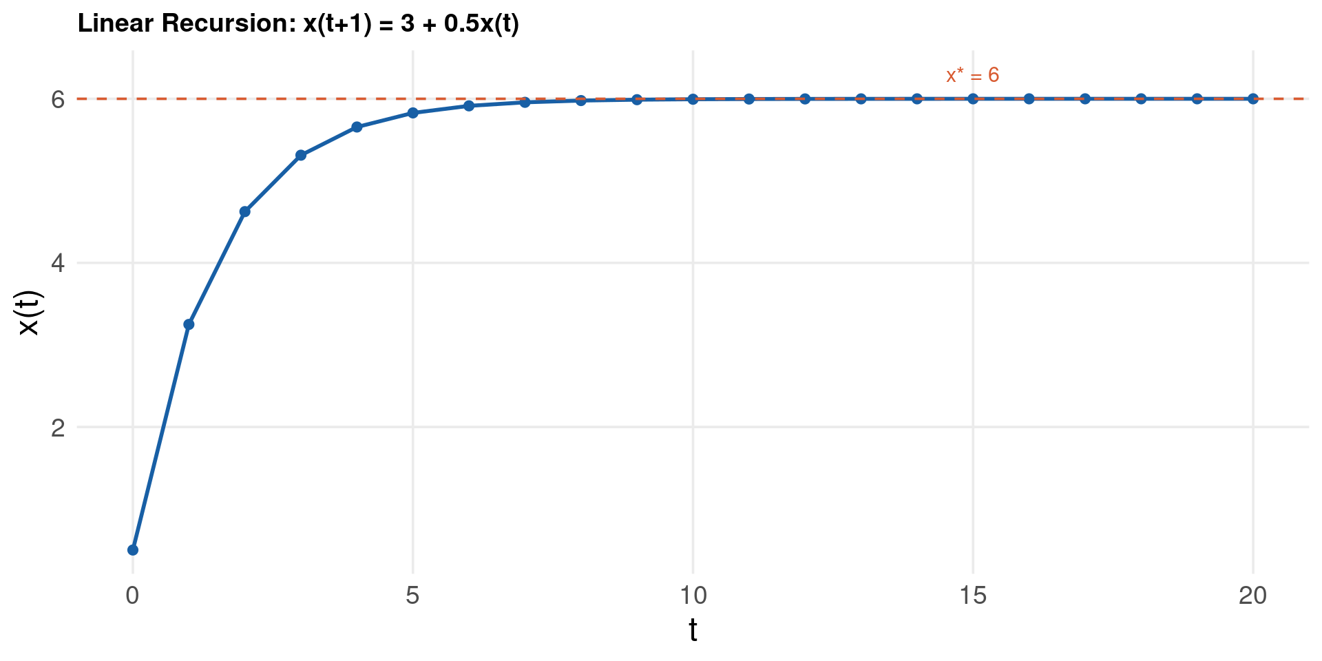
astavrak@uoi.gr · linkedin.com/in/astavrakoudis