Regularised Regression: A Machine Learning Toolkit for Econometrics

Lasso, Ridge, and Elastic Net
using R, Python & Stata

Athanassios Stavrakoudis

astavrak@uoi.gr

Applied Informatics and Computational Economics Lab

28 April 2026

Outline

•  Part I — Foundations: From TWFE to Machine Learning
•  Part II — Lasso: Sparse control selection · wagepan application · validity tests
•  Part III — Ridge: Dense shrinkage · wage equation with all controls
•  Part IV — Elastic Net: Grouped selection · occupation/industry structure
•  Running example throughout: wagepan union wage premium
•  Companion presentation: machine-learning-trees-ensembles-in-econometrics.Qmd covers Random Forests and XGBoost

Part I — Foundations

Prediction, Dimensionality, and Regularisation

Prediction vs Causal Inference — ① Prediction

Prediction: ML’s native goal

Find \(\hat{f}\) that minimises expected loss on new data:

\[\hat{f} = \arg\min_f \; \mathbb{E}\!\left[\ell\bigl(y, f(\mathbf{x})\bigr)\right]\]

• Coefficients are nuisance — only \(\hat{y}\) matters
• Regularisation, ensembling, and non-linearity are all fine
• Evaluation: out-of-sample RMSE, AUC, cross-validation
• High-\(p\) settings (\(p \gg n\)) are the norm, not the exception

Examples: credit scoring, spam detection, demand forecasting, house price estimation

What ML optimises for this goal: Minimise the generalisation error. Any model complexity is acceptable if it reduces out-of-sample loss. There is no requirement that the model be interpretable, identifiable, or consistent for any structural parameter.

Prediction vs Causal Inference — ② Causal Inference

Causal Inference: econometrics’ core goal

Identify a structural parameter \(\theta\) with valid inference:

\[y = \theta D + g(\mathbf{x}) + \varepsilon, \quad \mathbb{E}[\varepsilon \mid D, \mathbf{x}] = 0\]

• The coefficient \(\theta\) is the object of interest — not just a prediction weight
• Bias introduced by regularisation corrupts inference on \(\theta\)
• Evaluation: consistency, efficiency, correct coverage of CI
• Identification (exogeneity, IV, RDD, DiD) is not a data-fitting problem

Examples: policy evaluation, price elasticities, wage returns to schooling

⚠️  The Synthesis Goal of Modern Causal ML

Use ML's flexibility to estimate nuisance functions \(g_0(\mathbf{x}) = \mathbb{E}[y|\mathbf{x}]\) and \(m_0(\mathbf{x}) = \mathbb{E}[D|\mathbf{x}]\) nonparametrically —

while recovering valid \(\sqrt{n}\)-inference on the causal parameter \(\theta\) via Double/Debiased ML:

\[\hat\theta^{\text{DML}} = \left(\sum_{i\in I^c}\tilde{D}_i^2\right)^{-1}\sum_{i\in I^c}\tilde{D}_i\tilde{y}_i\]

\(\tilde{y}_i = y_i - \hat{g}(\mathbf{x}_i)\) and \(\tilde{D}_i = D_i - \hat{m}(\mathbf{x}_i)\) are the residuals from ML nuisance estimation. Regularisation bias in \(\hat{g}\) and \(\hat{m}\) does not contaminate \(\hat\theta\).

The Dimensionality Challenge

Classical OLS breaks down as the number of regressors \(p\) grows relative to \(n\):

\[\hat{\boldsymbol\beta}^{OLS} = (\mathbf{X}^\top \mathbf{X})^{-1}\mathbf{X}^\top \mathbf{y}\]

Setting	OLS behaviour	Remedy
\(p \ll n\), well-specified	Consistent, BLUE	None needed
\(p\) moderate, many nuisance	Overfits, poor OOS prediction	Regularisation
\(p > n\)	\((\mathbf{X}^\top\mathbf{X})\) singular — OLS undefined	Lasso / Ridge
\(p \gg n\), sparsity	Many true zeros; OLS has no power	Lasso + post-selection
Non-linear \(f(\mathbf{x})\)	Misspecification bias	Trees, kernels, nets

Econometric examples where \(p\) is large:

• Wage regressions with occupation × industry × region cells
• Gravity equations with bilateral fixed effects
• Price transmission with many retail outlets
• Programme evaluation with rich baseline survey controls

The Bias–Variance Decomposition

\[\text{MSE}(\hat\theta) = \underbrace{\text{Bias}^2(\hat\theta)}_{\text{systematic error}} + \underbrace{\text{Var}(\hat\theta)}_{\text{sampling noise}}\]

OLS minimises bias under correct specification — but variance explodes as \(p \to n\).

Regularisation deliberately introduces bias to sharply reduce variance. This trade-off is:

• worthwhile for prediction tasks
• requires correction (DML, post-selection) for causal inference

⚠️  The Curse: Training R² is Meaningless When p ≈ n

ISLR Figure 6.23 demonstrates this dramatically (James et al. 2023):

With \(n=20\) observations and completely noise predictors added one by one:

• Training \(R^2 \to 1\)  ←  perfect fit, zero signal
• Training MSE \(\to 0\)  ←  zero residuals, pure overfit
• Test MSE explodes  ←  catastrophic generalisation

ISLR §6.4.4 rule:

"One should never use sum of squared errors, \(p\)-values, \(R^2\), or other traditional measures of model fit on the training data as evidence of a good model fit in the high-dimensional setting."

Always report test-set MSE or cross-validation error. A model achieving \(R^2=1\) when \(p > n\) tells you nothing.

ISLR §6.4.4 pp. 266–267 — James, Witten, Hastie & Tibshirani (2023)

Where We Come From

You already know TWFE. It is powerful — but it has limits.
This presentation asks: what do we gain when we let the data choose the model?

From TWFE to Machine Learning — The Bridge

What you already know: Two-Way Fixed Effects (TWFE)

\[\text{lwage}_{it} = \alpha_i + \lambda_t + \beta\,\text{union}_{it} + \mathbf{x}_{it}'\boldsymbol\gamma + \varepsilon_{it}\]

TWFE is the workhorse of panel econometrics. It controls for all time-invariant unobservables (\(\alpha_i\)) and common shocks (\(\lambda_t\)). The wagepan dataset will be our running example throughout this presentation — the same data you used to estimate the union wage premium with TWFE.

Where TWFE hits a wall:

Problem	What happens	Consequence
Many controls (\(p\) large)	OLS is inconsistent; \((\mathbf{X}^\top\mathbf{X})^{-1}\) unreliable	Over-control bias; inflated SEs
Functional form	Linear specification may miss interactions, non-linearities	Omitted variable bias in a different form
Treatment heterogeneity	TWFE averages effects — may be negative-weighted	Aggregation bias (Callaway-Sant’Anna)
Pre-testing	Researcher selects controls ad hoc	Data snooping, publication bias

What Machine Learning adds:

ML tool	What it fixes	How
Lasso	High-dimensional control selection	Penalised regression — data-driven variable selection
Ridge	Correlated controls, dense signal	Shrinkage without zeroing
Elastic Net	Grouped correlated controls	Combined \(\ell_1 + \ell_2\) penalty
Random Forest	Non-linear nuisance functions	Nonparametric partitioning
DML	Valid \(\hat\beta\) after ML nuisance	Neyman orthogonality + cross-fitting

The key insight

ML is not a replacement for econometric models. It is a tool to build better nuisance estimates so that the final β̂ — the causal parameter you care about — is unbiased and efficient. The econometric model is still the Mincer equation; ML improves how you control for confounders.

Part II — Lasso

“Which of your 50 controls actually matter?”

You have education, experience, occupation, industry, region, and their interactions.
OLS keeps all of them. Lasso asks the data to choose.
What does it find?

Lasso — Econometric Framework

The problem: the Mincer equation on wagepan has up to \(p \approx 60\)–\(100\) candidate controls (occupation × industry × year interactions) for only \(n_{\text{eff}} \approx 545\) groups after removing fixed effects — too many to choose by hand.

TWFE with \(p\) controls:

\[\text{lwage}_{it} = \beta^{TWFE}\,\text{union}_{it} + \mathbf{x}_{it}'\boldsymbol\gamma + \alpha_i + \lambda_t + \varepsilon_{it}\]

This requires choosing which \(\mathbf{x}_{it}\) to include — typically ad hoc. Lasso replaces this with a data-driven selection rule.

Post-Lasso OLS — the estimator we will report:

\[\hat\beta^{PL} = (\mathbf{X}_{\hat{\mathcal{S}}}^\top\mathbf{X}_{\hat{\mathcal{S}}})^{-1}\mathbf{X}_{\hat{\mathcal{S}}}^\top\mathbf{y}\]

where \(\hat{\mathcal{S}} = \{j : \hat\beta_j^{\text{lasso}} \neq 0\}\) is the Lasso-selected support.

What \(\hat\beta^{PL}\) estimates: the union wage premium after controlling for the Lasso-selected set of covariates. This is still an OLS estimate — Lasso selects the model, OLS estimates the coefficients.

A caveat on causal interpretation

Post-Lasso OLS is not free of all biases. It controls only for the selected variables — omitted variable bias persists if relevant confounders are dropped. The causal interpretation of β̂_union still requires the CIA: \[ \text{union}_{it} \perp \varepsilon_{it} \mid \mathbf{x}_{it}, \alpha_i, \lambda_t \]

Regularised Regression — Lasso: Motivation

• ① Why variable selection matters
• ② What we gain and lose
• ③ Callouts

OLS with \(p\) predictors gives you \(p\) coefficients — even when most are noise.

In practice, economists face data with dozens or hundreds of candidate regressors: occupation × industry cells, interaction terms, polynomial expansions, control variables from rich surveys. Most of these have zero or negligible true effects. OLS keeps all of them, which inflates variance, masks the true signal, and makes results uninterpretable.

What we want: a method that automatically identifies which predictors matter and discards the rest.

Lasso (Tibshirani 1996) does exactly this. It adds a penalty on the sum of absolute values of coefficients (\(\ell_1\) norm):

\[\hat{\boldsymbol\beta}^{\text{lasso}} = \arg\min_{\boldsymbol\beta} \left\{\|\mathbf{y}-\mathbf{X}\boldsymbol\beta\|_2^2 + \lambda\|\boldsymbol\beta\|_1\right\}\]

The \(\ell_1\) penalty has a geometric property Ridge lacks: its constraint region (a diamond in 2D) has corners sitting exactly on the coordinate axes. When the OLS loss ellipsoid first touches the diamond it almost always hits a corner — setting one or more \(\hat\beta_j\) to exactly zero. This is automatic variable selection.

Econometric examples where sparsity holds: wage regressions (a few key skills dominate), programme evaluation (a few covariates confound), demand models (few cross-price elasticities are non-negligible).

What Lasso gives you:

Benefit	Mechanism
Automatic variable selection	Coefficients set to exactly zero
Interpretable model	Only the selected variables appear
Works when \(p > n\)	\(\ell_1\) constraint defines a unique solution even when OLS fails
Reduced prediction error	Variance reduction via sparsity
Foundation for causal ML	Post-double-selection IV, DML nuisance estimation

What Lasso costs you:

Cost	Why
Biased selected coefficients	\(\ell_1\) shrinks non-zero \(\hat\beta_j\) toward zero (not just zeros out)
No valid standard errors	Post-selection distribution is not the standard normal
Instability with correlated predictors	Lasso arbitrarily picks one from a correlated group
Inconsistent selection under corlinearity	Irrepresentability condition may fail
No causal interpretation without correction	Post-selection OLS (post-Lasso) or DML required

The solution to biased coefficients — post-Lasso OLS: After Lasso selects the support \(\hat{\mathcal{S}}\), re-run OLS using only the selected variables: \[\tilde{\boldsymbol\beta}^{\text{post}} = \arg\min_{\boldsymbol\beta:\,\text{supp}(\boldsymbol\beta)\subseteq\hat{\mathcal{S}}} \|\mathbf{y}-\mathbf{X}\boldsymbol\beta\|_2^2\] This removes the shrinkage bias on the selected coefficients. Under sparsity, \(\tilde{\boldsymbol\beta}^{\text{post}}\) is consistent at the \(\sqrt{n}\) rate.

⚠️  Lasso Selects — It Does Not Infer

No valid inference on Lasso-selected coefficients:

• \(\hat\beta_j^{\text{lasso}} \neq 0\)  ≠  "\(x_j\) has a causal effect"
• \(\hat\beta_j^{\text{lasso}} = 0\)  ≠  "\(x_j\) has no effect" (may be correlated with a selected variable)

For valid causal inference:

• PDS-Lasso (Belloni et al. 2014) — union selection then 2SLS/OLS
• DML (Chernozhukov et al. 2018) — Lasso as nuisance, OLS for \(\theta\)

📝  The Oracle Property

Fan & Li (2001); Zou (2006) — Adaptive Lasso:

Under sparsity + the irrepresentability condition:

"No excluded true predictor is too correlated with the included ones"

Lasso selects exactly the true support \(\mathcal{S}^*\) with probability \(\to 1\) as \(n \to \infty\) — as if an oracle had told you which variables matter.

Practical implication: Adaptive Lasso (weighted \(\ell_1\)) achieves the oracle property in finite samples more reliably. Use selection(adaptive) in Stata, hdm::rlasso() in R for inference applications.

💡  Three Methods to Choose \(\lambda\)

Method	Properties	When to use
Cross-validation (CV)	Minimises prediction MSE; selects more variables	Prediction tasks; default choice
Adaptive Lasso	Re-weighted; sparser than CV; oracle property	Variable selection for inference
Plugin (theory-driven)	Dominates estimation noise; sparsest	Formal post-selection inference, DML

R: cv.glmnet(alpha=1) / hdm::rlasso()  |  Stata: selection(cv) / selection(adaptive) / selection(plugin)

📝  Bayesian Interpretation of Lasso (ISLR §6.2.2)

Ridge and Lasso both have a Bayesian interpretation as MAP estimators:

Method	Prior on \(\beta_j\)	Shape	Why zeros?
Ridge	\(\mathcal{N}(0,\sigma^2/\lambda)\)	Smooth bell — flat at zero	Rare: prior gives low density near zero
Lasso	Double-exponential / Laplace	Sharp spike at zero	Prior expects most \(\beta_j\) to be exactly zero

The Laplace prior is \(p(\beta_j) \propto \exp(-\lambda|\beta_j|)\). Its sharp peak at zero means the prior strongly expects sparse coefficients — which is why the Lasso posterior mode produces exact zeros.

Ridge has a Gaussian prior: flat and wide at zero, so small but non-zero coefficients are plausible, and the posterior mode is never exactly zero.

ISLR §6.2.2 pp. 249–250, Figure 6.11 — James, Witten, Hastie & Tibshirani (2023)

Regularised Regression — Lasso: Mathematics I

Primal problem (\(\ell_1\)-penalised least squares):

\[\hat{\boldsymbol\beta}^{\text{lasso}} = \arg\min_{\boldsymbol\beta} \underbrace{\|\mathbf{y}-\mathbf{X}\boldsymbol\beta\|_2^2}_{\text{fit}} + \lambda\underbrace{\|\boldsymbol\beta\|_1}_{\text{sparsity penalty}} \qquad \lambda \geq 0\]

No closed form — unlike Ridge, the \(\ell_1\) penalty is non-differentiable at zero.

Equivalent constrained form (Lagrangian duality):

\[\hat{\boldsymbol\beta}^{\text{lasso}} = \arg\min_{\boldsymbol\beta}\|\mathbf{y}-\mathbf{X}\boldsymbol\beta\|_2^2 \quad\text{s.t.}\quad \|\boldsymbol\beta\|_1 \leq t(\lambda)\]

The \(\ell_1\) ball is a diamond — the OLS loss ellipsoid touches the diamond at a corner on a coordinate axis, setting that coefficient to exactly zero. This is the geometric source of sparsity.

Soft-thresholding — the scalar solution:

For orthogonal \(\mathbf{X}\) (or equivalently, when solving coordinate-by-coordinate) the Lasso solution for \(\beta_j\) has a closed form:

\[\hat\beta_j^{\text{lasso}} = S_{\lambda/2}(\hat\beta_j^{\text{OLS}}) \equiv \text{sign}(\hat\beta_j^{\text{OLS}})\cdot\max\!\left(|\hat\beta_j^{\text{OLS}}| - \tfrac{\lambda}{2},\; 0\right)\]

This soft-thresholding operator \(S_{\lambda/2}(\cdot)\) (the knee sits at \(\lambda/2\) because the loss \(\|\mathbf{y}-\mathbf{X}\boldsymbol\beta\|_2^2\) is written without the \(\tfrac{1}{2}\) factor — cf. the \(\tfrac{2}{n}\) in the KKT conditions below and the Elastic Net coordinate updates):

• Shrinks \(\hat\beta_j^{\text{OLS}}\) toward zero by \(\lambda/2\) (the shrinkage effect, shared with Ridge)
• Sets it to exactly zero if \(|\hat\beta_j^{\text{OLS}}| \leq \lambda/2\) (the selection effect, unique to Lasso)

Key properties:

Property	Result
Unique solution?	Yes if \(\mathbf{X}^\top\mathbf{X}\) is positive definite; otherwise a convex set of solutions
Exact zeros (sparsity)?	Yes — the defining feature
Scale-invariant?	No — always standardise \(\mathbf{X}\) first
Consistent as \(n\to\infty\)?	Yes under irrepresentability condition
Computational cost	Coordinate descent: \(\mathcal{O}(np)\) per \(\lambda\)

📝  Coordinate Descent (glmnet, Stata)

Cycle over \(j = 1,\ldots,p\); for each \(j\), fix all other \(\hat\beta_{k\neq j}\) and apply the soft-thresholding update:

\[\hat\beta_j \leftarrow S_\lambda\!\left(\frac{1}{n}\mathbf{x}_j^\top(\mathbf{y} - \mathbf{X}_{-j}\hat{\boldsymbol\beta}_{-j})\right)\]

Repeat until convergence. This is how all modern Lasso implementations work — glmnet in R, LassoCV in scikit-learn, and lasso in Stata.

⚠️  Lasso and Ridge are NOT Scale-Invariant

OLS is scale equivariant: multiplying \(X_j\) by \(c\) divides \(\hat\beta_j^{OLS}\) by \(c\), so \(X_j\hat\beta_j\) is unchanged.

Lasso and Ridge are not. The penalty \(\lambda\|\boldsymbol\beta\|_1\) applies the same \(\lambda\) to all coefficients regardless of the scale of \(X_j\). Measuring income in dollars vs thousands of dollars gives substantially different coefficient estimates.

Consequence: always standardise before penalising:

\[\tilde{x}_{ij} = \frac{x_{ij}}{\hat\sigma_j}, \quad \hat\sigma_j = \sqrt{\tfrac{1}{n}\sum_i(x_{ij}-\bar x_j)^2}\]

In practice:

• glmnet (R): standardises by default (standardize=TRUE)
• scikit-learn: does NOT standardise — use a Pipeline with StandardScaler
• Stata lasso: standardises by default

ISLR §6.2.1, p. 239 — James, Witten, Hastie & Tibshirani (2023)

Regularised Regression — Lasso: Mathematics II

The regularisation path — how \(\hat{\boldsymbol\beta}^{\text{lasso}}(\lambda)\) evolves:

As \(\lambda\) decreases from \(\lambda_{\max}\) (all coefficients zero) toward \(0\) (OLS), variables enter the model one at a time:

\[\lambda_{\max} = \max_j |\mathbf{x}_j^\top\mathbf{y}|/n\]

At \(\lambda_{\max}\): \(\hat{\boldsymbol\beta} = \mathbf{0}\). As \(\lambda\) decreases, the predictor most correlated with the current residual enters. This piecewise-linear path is traced by the LARS algorithm (Efron et al. 2004).

KKT conditions — the stationarity conditions that characterise the solution:

\[\frac{2}{n}\mathbf{x}_j^\top(\mathbf{y}-\mathbf{X}\hat{\boldsymbol\beta}) = \lambda\cdot\hat{s}_j \qquad\text{where}\qquad \hat{s}_j \in \begin{cases} \{\text{sign}(\hat\beta_j)\} & \hat\beta_j \neq 0 \\ [-1,1] & \hat\beta_j = 0 \end{cases}\]

Reading the KKT conditions:

• For a selected variable (\(\hat\beta_j \neq 0\)): its correlation with the current residual exactly equals \(\pm\lambda\)
• For an unselected variable (\(\hat\beta_j = 0\)): its correlation with the residual is strictly less than \(\lambda\) in absolute value

Post-Lasso OLS — removing the shrinkage bias:

Let \(\hat{\mathcal{S}} = \{j : \hat\beta_j^{\text{lasso}} \neq 0\}\) be the selected set. Then:

\[\tilde{\boldsymbol\beta}^{\text{post}} = (\mathbf{X}_{\hat{\mathcal{S}}}^\top\mathbf{X}_{\hat{\mathcal{S}}})^{-1}\mathbf{X}_{\hat{\mathcal{S}}}^\top\mathbf{y}\]

This OLS fit on the selected subset eliminates Lasso’s shrinkage bias. Post-Lasso OLS is the default reported coefficient in Stata’s lasso command. In glmnet it requires a second lm() call on the selected variables.

📝  Belloni & Chernozhukov (2013)

Under sparsity, post-Lasso OLS achieves the same convergence rate as Lasso but with a smaller bias constant.

In linear models, post-Lasso OLS typically outperforms the penalised Lasso coefficients for both prediction and estimation.

Reference: Belloni, Chernozhukov & Wang (2012); Belloni et al. (2013) Bernoulli 19(2): 521–547.

Lasso — Optimisation: Coordinate Descent

The Lasso objective has no closed form — the \(\ell_1\) penalty is non-differentiable at \(0\) — so it is solved numerically. glmnet, scikit-learn, and Stata all use the same workhorse: cyclic coordinate descent, minimising

\[Q(\beta)=\frac{1}{2n}\sum_{i=1}^{n}\Big(y_i-\textstyle\sum_k x_{ik}\beta_k\Big)^2+\lambda\sum_k|\beta_k|\]

one coordinate at a time, holding the others fixed. For standardised predictors (\(\tfrac1n\sum_i x_{ij}^2=1\)) the coordinate-\(j\) minimiser is the soft-thresholding update

\[\beta_j \leftarrow S\!\big(z_j,\,\lambda\big)\]

\[z_j=\frac1n\sum_{i=1}^{n} x_{ij}\,r_i^{(-j)}, \qquad r^{(-j)}=y-\sum_{k\neq j}x_k\beta_k\]

\[S(z,\gamma)=\operatorname{sign}(z)\,\max(|z|-\gamma,0)\]

where \(r^{(-j)}\) is the partial residual. The threshold \(\lambda\) is exactly what produces sparsity: any coordinate with \(|z_j|\le\lambda\) collapses to \(0\). Solvers sweep \(j=1,\dots,p\) until \(\max_j|\beta_j^{\text{new}}-\beta_j^{\text{old}}|<\texttt{tol}\), and compute the whole \(\lambda\)-path from large to small with warm starts (each \(\lambda\) initialised at the previous solution) — which is what makes the path cheap.

The algorithm is due to Friedman, Hastie, Höfling & Tibshirani (2007), “Pathwise coordinate optimization,” Ann. Appl. Stat. doi:10.1214/07-AOAS131; and Friedman, Hastie & Tibshirani (2010), “Regularization paths for generalized linear models via coordinate descent,” J. Stat. Soft. doi:10.18637/jss.v033.i01.

Lasso — Coordinate Descent: Code

The same algorithm from scratch and via each library, on a few standardised wagepan controls. glmnet, scikit-learn, and Stata all run cyclic coordinate descent internally.

• R
• Python
• Stata

wp <- wagepan

# Standardised design from a few wagepan controls (coordinate descent needs
# comparable scales); centre the outcome so the intercept drops out.
vars <- c("educ", "exper", "expersq", "married", "union", "hours")
vars <- intersect(vars, names(wp))
X <- scale(as.matrix(wp[, vars]))
y <- wp$lwage - mean(wp$lwage)
n <- nrow(X)
p <- ncol(X)

# Soft-thresholding operator: S(z, g) = sign(z) * max(|z| - g, 0)
soft_threshold <- function(z, g) sign(z) * pmax(abs(z) - g, 0)

# Cyclic coordinate descent for the Lasso (glmnet objective (1/2n)RSS + lambda*||b||_1)
lasso_cd <- function(X, y, lambda, max_iter = 1000L, tol = 1e-7) {
  n <- nrow(X)
  p <- ncol(X)
  beta <- rep(0, p)                                  # warm start at zero
  for (iter in seq_len(max_iter)) {
    beta_old <- beta
    for (j in seq_len(p)) {
      r_j <- y - X[, -j, drop = FALSE] %*% beta[-j]  # partial residual
      z_j <- sum(X[, j] * r_j) / n                   # (1/n) x_j' r_j  (x_j standardised)
      beta[j] <- soft_threshold(z_j, lambda)
    }
    if (max(abs(beta - beta_old)) < tol) break       # convergence check
  }
  list(beta = beta, iters = iter)
}

fit <- lasso_cd(X, y, lambda = 0.05)
cat(sprintf("From-scratch coordinate descent: converged in %d sweeps\n", fit$iters))

From-scratch coordinate descent: converged in 8 sweeps

print(round(setNames(fit$beta, vars), 4))

   educ   exper expersq married   union   hours 
 0.1080  0.0717  0.0000  0.0357  0.0253  0.0000 

# glmnet runs the same algorithm; these are its convergence controls:
library(glmnet)
g <- glmnet(X, y, alpha = 1, lambda = 0.05,
            standardize = FALSE,   # X already standardised above
            thresh = 1e-7,         # convergence threshold (default 1e-7)
            maxit = 1e5)           # max passes over coordinates (default 1e5)
cat("glmnet coefficients (same lambda):\n")

glmnet coefficients (same lambda):

print(round(as.numeric(coef(g))[-1], 4))

[1] 0.1081 0.0717 0.0000 0.0357 0.0253 0.0000

import numpy as np
import wooldridge as woo
from sklearn.linear_model import Lasso

wp = woo.dataWoo("wagepan")
cols = [c for c in ["educ", "exper", "expersq", "married", "union", "hours"]
        if c in wp.columns]
X = wp[cols].to_numpy(dtype=float)
X = (X - X.mean(0)) / X.std(0)                 # standardise: comparable scales
y = wp["lwage"].to_numpy() - wp["lwage"].mean()  # centre: intercept drops out
n, p = X.shape

def soft_threshold(z, g):
    return np.sign(z) * max(abs(z) - g, 0.0)

def lasso_cd(X, y, lam, max_iter=1000, tol=1e-7):
    n, p = X.shape
    beta = np.zeros(p)                          # warm start at zero
    for it in range(max_iter):
        beta_old = beta.copy()
        for j in range(p):
            r_j = y - X @ beta + X[:, j] * beta[j]   # partial residual
            z_j = X[:, j] @ r_j / n
            beta[j] = soft_threshold(z_j, lam)
        if np.max(np.abs(beta - beta_old)) < tol:
            break
    return beta, it + 1

beta, iters = lasso_cd(X, y, lam=0.05)
print(f"From-scratch coordinate descent: converged in {iters} sweeps")

From-scratch coordinate descent: converged in 8 sweeps

print({v: round(b, 4) for v, b in zip(cols, beta)})

{'educ': np.float64(0.1081), 'exper': np.float64(0.0717), 'expersq': np.float64(0.0), 'married': np.float64(0.0357), 'union': np.float64(0.0253), 'hours': np.float64(-0.0)}

# scikit-learn runs the same algorithm; these are its convergence controls:
m = Lasso(alpha=0.05, fit_intercept=False, max_iter=10000, tol=1e-7)
m.fit(X, y)

Lasso(alpha=0.05, fit_intercept=False, max_iter=10000, tol=1e-07)

In a Jupyter environment, please rerun this cell to show the HTML representation or trust the notebook.
On GitHub, the HTML representation is unable to render, please try loading this page with nbviewer.org.

print("sklearn coefficients (same alpha):", np.round(m.coef_, 4))

sklearn coefficients (same alpha): [ 0.1081  0.0717  0.      0.0357  0.0253 -0.    ]

# A "ConvergenceWarning: Objective did not converge" means max_iter was hit
# before tol — raise max_iter, loosen tol, or check standardisation.

frause wagepan, clear

* lasso/elasticnet minimise the penalised objective by COORDINATE DESCENT and
* standardise covariates internally (mean 0, sd 1), which also removes the
* constant from the penalised problem.
lasso linear lwage educ exper expersq married union hours, ///
    selection(cv, folds(10)) rseed(14159) ///
    tolerance(1e-7)            // stop when the coefficient vector changes by < tol
lassocoef
* Notes on convergence controls:
*  - the lambda path stops early when the deviance change falls below stop(#);
*  - lassopack's rlasso/cvlasso expose the shooting algorithm directly via
*    tolopt() (default 1e-10) and maxiter() (default 10000).

10-fold cross-validation with 100 lambdas ...
Grid value 1:     lambda = .1342726   no. of nonzero coef. = 0
Folds: 1...5....10   CVF = .2836261
Grid value 2:     lambda = .1223442   no. of nonzero coef. = 1
Folds: 1...5....10   CVF = .2810071
Grid value 3:     lambda = .1114755   no. of nonzero coef. = 1
Folds: 1...5....10   CVF = .2784354
Grid value 4:     lambda = .1015723   no. of nonzero coef. = 3
Folds: 1...5....10   CVF = .2742572
Grid value 5:     lambda = .0925489   no. of nonzero coef. = 3
Folds: 1...5....10   CVF = .2684452
Grid value 6:     lambda = .0843271   no. of nonzero coef. = 3
Folds: 1...5....10   CVF =  .263573
Grid value 7:     lambda = .0768357   no. of nonzero coef. = 3
Folds: 1...5....10   CVF = .2594574
Grid value 8:     lambda = .0700099   no. of nonzero coef. = 4
Folds: 1...5....10   CVF = .2554415
Grid value 9:     lambda = .0637904   no. of nonzero coef. = 4
Folds: 1...5....10   CVF =  .251874
Grid value 10:    lambda = .0581234   no. of nonzero coef. = 4
Folds: 1...5....10   CVF = .2489127
Grid value 11:    lambda = .0529599   no. of nonzero coef. = 4
Folds: 1...5....10   CVF = .2464547
Grid value 12:    lambda = .0482551   no. of nonzero coef. = 4
Folds: 1...5....10   CVF = .2444144
Grid value 13:    lambda = .0439682   no. of nonzero coef. = 4
Folds: 1...5....10   CVF =  .242721
Grid value 14:    lambda = .0400622   no. of nonzero coef. = 4
Folds: 1...5....10   CVF = .2413155
Grid value 15:    lambda = .0365032   no. of nonzero coef. = 4
Folds: 1...5....10   CVF =  .240149
Grid value 16:    lambda = .0332604   no. of nonzero coef. = 4
Folds: 1...5....10   CVF = .2391808
Grid value 17:    lambda = .0303056   no. of nonzero coef. = 4
Folds: 1...5....10   CVF = .2383786
Grid value 18:    lambda = .0276133   no. of nonzero coef. = 4
Folds: 1...5....10   CVF = .2377318
Grid value 19:    lambda = .0251602   no. of nonzero coef. = 5
Folds: 1...5....10   CVF =  .237171
Grid value 20:    lambda = .0229251   no. of nonzero coef. = 5
Folds: 1...5....10   CVF = .2365673
Grid value 21:    lambda = .0208885   no. of nonzero coef. = 5
Folds: 1...5....10   CVF = .2360062
Grid value 22:    lambda = .0190328   no. of nonzero coef. = 5
Folds: 1...5....10   CVF = .2355404
Grid value 23:    lambda =  .017342   no. of nonzero coef. = 5
Folds: 1...5....10   CVF = .2351536
Grid value 24:    lambda = .0158014   no. of nonzero coef. = 5
Folds: 1...5....10   CVF = .2348325
Grid value 25:    lambda = .0143976   no. of nonzero coef. = 5
Folds: 1...5....10   CVF = .2345658
Grid value 26:    lambda = .0131186   no. of nonzero coef. = 5
Folds: 1...5....10   CVF = .2343445
Grid value 27:    lambda = .0119532   no. of nonzero coef. = 5
Folds: 1...5....10   CVF = .2341607
Grid value 28:    lambda = .0108913   no. of nonzero coef. = 5
Folds: 1...5....10   CVF =  .234008
Grid value 29:    lambda = .0099237   no. of nonzero coef. = 5
Folds: 1...5....10   CVF = .2338813
Grid value 30:    lambda = .0090421   no. of nonzero coef. = 5
Folds: 1...5....10   CVF = .2337761
Grid value 31:    lambda = .0082388   no. of nonzero coef. = 5
Folds: 1...5....10   CVF = .2336888
Grid value 32:    lambda = .0075069   no. of nonzero coef. = 5
Folds: 1...5....10   CVF = .2336162
Grid value 33:    lambda =   .00684   no. of nonzero coef. = 5
Folds: 1...5....10   CVF =  .233556
Grid value 34:    lambda = .0062324   no. of nonzero coef. = 5
Folds: 1...5....10   CVF =  .233506
Grid value 35:    lambda = .0056787   no. of nonzero coef. = 5
Folds: 1...5....10   CVF = .2334644
Grid value 36:    lambda = .0051742   no. of nonzero coef. = 5
Folds: 1...5....10   CVF = .2334299
Grid value 37:    lambda = .0047146   no. of nonzero coef. = 5
Folds: 1...5....10   CVF =  .233401
Grid value 38:    lambda = .0042957   no. of nonzero coef. = 6
Folds: 1...5....10   CVF = .2333535
Grid value 39:    lambda = .0039141   no. of nonzero coef. = 6
Folds: 1...5....10   CVF = .2332141
Grid value 40:    lambda = .0035664   no. of nonzero coef. = 6
Folds: 1...5....10   CVF = .2330798
Grid value 41:    lambda = .0032496   no. of nonzero coef. = 6
Folds: 1...5....10   CVF = .2329424
Grid value 42:    lambda = .0029609   no. of nonzero coef. = 6
Folds: 1...5....10   CVF = .2328283
Grid value 43:    lambda = .0026979   no. of nonzero coef. = 6
Folds: 1...5....10   CVF = .2327336
Grid value 44:    lambda = .0024582   no. of nonzero coef. = 6
Folds: 1...5....10   CVF =  .232655
Grid value 45:    lambda = .0022398   no. of nonzero coef. = 6
Folds: 1...5....10   CVF = .2325897
Grid value 46:    lambda = .0020408   no. of nonzero coef. = 6
Folds: 1...5....10   CVF = .2325354
Grid value 47:    lambda = .0018595   no. of nonzero coef. = 6
Folds: 1...5....10   CVF = .2324904
Grid value 48:    lambda = .0016943   no. of nonzero coef. = 6
Folds: 1...5....10   CVF =  .232453
Grid value 49:    lambda = .0015438   no. of nonzero coef. = 6
Folds: 1...5....10   CVF =  .232422
Grid value 50:    lambda = .0014067   no. of nonzero coef. = 6
Folds: 1...5....10   CVF = .2323962
Grid value 51:    lambda = .0012817   no. of nonzero coef. = 6
Folds: 1...5....10   CVF = .2323748
Grid value 52:    lambda = .0011678   no. of nonzero coef. = 6
Folds: 1...5....10   CVF =  .232357
Grid value 53:    lambda = .0010641   no. of nonzero coef. = 6
Folds: 1...5....10   CVF = .2323423
Grid value 54:    lambda = .0009696   no. of nonzero coef. = 6
Folds: 1...5....10   CVF =   .23233
Grid value 55:    lambda = .0008834   no. of nonzero coef. = 6
Folds: 1...5....10   CVF = .2323199
Grid value 56:    lambda = .0008049   no. of nonzero coef. = 6
Folds: 1...5....10   CVF = .2323114
Grid value 57:    lambda = .0007334   no. of nonzero coef. = 6
Folds: 1...5....10   CVF = .2323044
Grid value 58:    lambda = .0006683   no. of nonzero coef. = 6
Folds: 1...5....10   CVF = .2322986
Grid value 59:    lambda = .0006089   no. of nonzero coef. = 6
Folds: 1...5....10   CVF = .2322937
Grid value 60:    lambda = .0005548   no. of nonzero coef. = 6
Folds: 1...5....10   CVF = .2322897
Grid value 61:    lambda = .0005055   no. of nonzero coef. = 6
Folds: 1...5....10   CVF = .2322863
Grid value 62:    lambda = .0004606   no. of nonzero coef. = 6
Folds: 1...5....10   CVF = .2322836
Grid value 63:    lambda = .0004197   no. of nonzero coef. = 6
Folds: 1...5....10   CVF = .2322813
Grid value 64:    lambda = .0003824   no. of nonzero coef. = 6
Folds: 1...5....10   CVF = .2322794
Grid value 65:    lambda = .0003484   no. of nonzero coef. = 6
Folds: 1...5....10   CVF = .2322778
Grid value 66:    lambda = .0003175   no. of nonzero coef. = 6
Folds: 1...5....10   CVF = .2322764
Grid value 67:    lambda = .0002893   no. of nonzero coef. = 6
Folds: 1...5....10   CVF = .2322753
Grid value 68:    lambda = .0002636   no. of nonzero coef. = 6
Folds: 1...5....10   CVF = .2322744
Grid value 69:    lambda = .0002402   no. of nonzero coef. = 6
Folds: 1...5....10   CVF = .2322737
Grid value 70:    lambda = .0002188   no. of nonzero coef. = 6
Folds: 1...5....10   CVF =  .232273
Grid value 71:    lambda = .0001994   no. of nonzero coef. = 6
Folds: 1...5....10   CVF = .2322725
... change in deviance stopping tolerance reached ... last lambda selected
Minimum of CV function not found; lambda selected based on stop() stopping criterion.

Lasso linear model                          No. of obs        =      4,360
                                            No. of covariates =          6
Selection: Cross-validation                 No. of CV folds   =         10

--------------------------------------------------------------------------
         |                                No. of      Out-of-      CV mean
         |                               nonzero       sample   prediction
      ID |     Description      lambda     coef.    R-squared        error
---------+----------------------------------------------------------------
       1 |    first lambda    .1342726         0      -0.0001     .2836261
      70 |   lambda before    .0002188         6       0.1810      .232273
    * 71 | selected lambda    .0001994         6       0.1810     .2322725
--------------------------------------------------------------------------
* lambda selected by cross-validation.
Note: Minimum of CV function not found; lambda selected based on stop()
      stopping criterion.


------------------------
             |  active  
-------------+----------
        educ |     x    
       exper |     x    
     expersq |     x    
     married |     x    
       union |     x    
       hours |     x    
       _cons |     x    
------------------------
Legend:
  b - base level
  e - empty cell
  o - omitted
  x - estimated

⚠️  Convergence pitfalls

• Standardise first. Coordinate descent assumes comparable scales; all three libraries standardise internally by default and back-transform. Running on raw-scale data with standardisation off slows or breaks convergence.
• Non-convergence warnings (scikit-learn's ConvergenceWarning; glmnet silently hitting maxit) mean the sweep limit was reached before tol. Raise max_iter/maxit, loosen tol, or rescale.
• Correlated predictors make coordinate descent zig-zag — it can only move one of a correlated pair per sweep — so it needs more iterations. This is exactly the wagepan occupation/industry-dummy situation, and the motivation for Elastic Net.
• \(\lambda\) too small (approaching OLS with \(p\approx n\)) is the slowest, least stable regime; the path's warm starts are what keep it tractable.

Lasso — When It Excels and When It Fails

• ✓ Use Lasso when
• ✗ Do NOT use Lasso when

1. Sparse DGP — few truly relevant predictors — If the true model has \(s \ll p\) non-zero coefficients (e.g. a handful of key policy variables among hundreds of controls), Lasso recovers the sparse structure. Ridge would needlessly retain all \(p\) noisy variables.

2. High-dimensional control selection (\(p > n\)) — OLS is not defined. Lasso produces a unique sparse solution and selects the most relevant subset of controls.

3. Post-double-selection IV (Belloni, Chernozhukov & Hansen) — Lasso selects controls in both the outcome and treatment equations; the union set is used in 2SLS. Directly implemented in R’s hdm::rlassoIV() and Stata’s pdslasso.

4. DML nuisance estimation under sparsity — When the nuisance function \(g(\mathbf{x}) = \mathbb{E}[y|\mathbf{X}]\) is sparse, Lasso achieves the product-rate condition \(\|\hat{g}-g_0\|_2\cdot\|\hat{m}-m_0\|_2 = o(n^{-1/2})\) needed for valid DML inference.

5. Interpretability of the selected model — A sparse model with 8 selected predictors from 50 candidates is far easier to interpret than OLS with 50 noisy coefficients.

💡  Adaptive Lasso (Zou 2006)

The adaptive Lasso upweights the penalty for small OLS coefficients:

\[\hat\beta^{\text{adapt}} = \arg\min_\beta \left\{\|\mathbf{y}-\mathbf{X}\beta\|^2 + \lambda\sum_j \hat\omega_j|\beta_j|\right\}\]

where \(\hat\omega_j = 1/|\hat\beta_j^{\text{OLS}}|^\gamma\). Heavy penalties on small coefficients drive them to zero.

Oracle property: asymptotically selects exactly the true support \(\mathcal{S}^*\) and is \(\sqrt{n}\)-consistent on the selected set. In Stata: lasso ... , selection(adaptive).

1. Dense signal — most predictors contribute small effects — Lasso zeros out genuinely non-zero but small coefficients. Ridge or Elastic Net is better when all predictors matter a little.

2. Highly correlated predictors (grouped variables) — Lasso arbitrarily picks one variable from a correlated group and discards the others — even if all are relevant. Elastic Net with \(\alpha < 1\) handles this correctly.

3. You need valid confidence intervals on \(\hat\beta_j\) — Lasso’s post-selection distribution is not normal. Do not report \(t\)-statistics from a Lasso fit. Use post-double-selection Lasso or DML.

4. \(n \gg p\), no sparsity — OLS is already efficient. Lasso adds selection bias with no gain.

5. Prediction only, dense signal — For pure prediction with a dense DGP, Ridge typically achieves lower MSE because it spreads regularisation across all directions rather than zeroing out genuine signal.

⚠️  Lasso vs Ridge: The Fundamental Choice

DGP	Best method	Why
Sparse — few large effects, many true zeros	Lasso	Sets small coefficients to exactly zero; variable selection
Dense — many small effects	Ridge	Keeps all predictors; no arbitrary zeroing
Unknown	Elastic Net	Includes both; CV selects \(\alpha\)

Lasso — Key Functions: Fitting

Before running the steps: a map of the fitting call in each language, annotated argument by argument. The cross-validation and extraction functions follow on the next slide.

• R — glmnet
• Python — scikit-learn
• Stata — lasso

Package: glmnet (Friedman, Hastie & Tibshirani)

fit <- glmnet(
  X,                              # numeric MATRIX (n × p), NOT a data.frame
  y,                              # response vector, length n
  family      = "gaussian",       # "gaussian" for linear; "binomial" for logit (optional)
  alpha       = 1,                # 1 = Lasso, 0 = Ridge, (0,1) = Elastic Net
  lambda      = NULL,             # NULL → glmnet auto-computes the λ path from data
  nlambda     = 100,              # number of λ values on that path (default 100, optional)
  standardize = TRUE              # scale X to unit SD before penalising (mandatory)
)
# fit$beta   → p × nlambda sparse matrix of coefficients (one column per λ)
# fit$lambda → the decreasing sequence of λ values actually used
# fit$df     → number of non-zero coefficients at each λ

Math connection: glmnet(alpha=1) solves \(\hat{\boldsymbol\beta}(\lambda) = \arg\min \tfrac{1}{2n}\|\mathbf{y}-\mathbf{X}\boldsymbol\beta\|_2^2 + \lambda\|\boldsymbol\beta\|_1\) for all nlambda values of \(\lambda\) simultaneously via coordinate descent, exploiting warm starts along the path.

Package: sklearn.linear_model

from sklearn.linear_model import Lasso

fit = Lasso(
    alpha        = 0.05,      # the single λ (sklearn calls it alpha); NOT cross-validated here
    fit_intercept= True,      # estimate an unpenalised intercept (default True)
    max_iter     = 10000,     # coordinate-descent sweep budget; raise on ConvergenceWarning
    tol          = 1e-4,      # duality-gap convergence tolerance (default 1e-4)
    selection    = "cyclic"   # "cyclic" or "random" (random often converges faster)
)
fit.fit(X, y)                 # X: numpy array (n × p); y: numpy array (n,)
# fit.coef_      → coefficient array length p (exact zeros = not selected)
# fit.intercept_ → fitted intercept
# NOTE: Lasso does NOT standardise — wrap StandardScaler in a Pipeline

Math connection: a single alpha \(=\lambda\). coef_[j] == 0 means \(\hat\beta_j\) was soft-thresholded to exactly zero; non-zero entries are selected but still shrunk toward zero.

Command: lasso linear (Stata 16+)

lasso linear y x1-x50,           ///
    selection(none)              /// fit at a supplied λ grid without CV selection
    grid(100)                    /// number of λ values on the path (default 100)
    nolog                        // suppress the iteration log
* By default Stata standardises covariates internally and back-transforms.
* lassoknots, display(nonzero)   // which variables enter at each λ on the path

Math connection: Stata minimises \(\tfrac{1}{2n}\|\mathbf{y}-\mathbf{X}\boldsymbol\beta\|^2 + \lambda\sum_j\omega_j|\beta_j|\) by coordinate descent. selection(none) fits the whole path; CV selection (next slide) chooses the operating \(\lambda\).

Lasso — Key Functions: Cross-Validation & Extraction

Fitting gives the whole \(\lambda\)-path; cross-validation picks the operating point, then you extract coefficients and predictions.

• R — glmnet
• Python — scikit-learn
• Stata — lasso

cv_fit <- cv.glmnet(
  X,                              # same matrix as the fit
  y,                              # same response vector
  alpha        = 1,               # 1 = Lasso (match the fit)
  nfolds       = 10,              # number of CV folds (default 10)
  type.measure = "mse"            # select λ by out-of-fold mean squared error
)
# cv_fit$lambda.min → λ minimising CV-MSE      (more variables, best prediction)
# cv_fit$lambda.1se → largest λ within 1 SE    (sparser, preferred for inference)
# cv_fit$cvm        → vector of CV-MSE per λ
# cv_fit$cvsd       → vector of CV-MSE standard errors per λ

# Extract coefficients at the chosen λ:
b   <- coef(cv_fit, s = "lambda.min")   # sparse (p+1) vector, intercept first
sel <- which(b[-1] != 0)                # indices of selected variables

# Predict on new data:
yhat <- predict(cv_fit, newx = X_test, s = "lambda.min")

Math connection: lambda.min and lambda.1se are the two standard operating points on the CV curve; lambda.1se trades a little fit for a sparser, more stable model.

from sklearn.linear_model import LassoCV
from sklearn.preprocessing import StandardScaler
from sklearn.pipeline import Pipeline

# LassoCV fits the path AND cross-validates λ in one call:
pipe = Pipeline([
    ("scaler", StandardScaler()),       # X → zero mean, unit SD (training stats only)
    ("lasso",  LassoCV(
        n_alphas     = 100,             # size of the λ grid (auto-computed, large→small)
        cv           = 10,              # number of CV folds
        max_iter     = 10000,           # raise if a ConvergenceWarning appears
        random_state = 14159
    ))
])
pipe.fit(X_train, y_train)
model = pipe.named_steps["lasso"]
# model.alpha_    → selected λ (sklearn's "alpha")
# model.coef_     → coefficients (exact zero = not selected)
# model.mse_path_ → (n_alphas × cv) matrix of fold MSEs

Math connection: alpha_ \(=\hat\lambda\) from cross-validation; everything else is read off the fitted model.

lasso linear y x1-x50,           ///
    selection(cv, folds(10))     /// 10-fold CV to select λ  [or: adaptive, plugin]
    rseed(14159)                 /// reproducible fold assignment
    nolog                        // suppress iteration log

* Post-estimation:
lassoinfo                                    // λ*, no. of non-zero coefs, CV-MSE
lassocoef, display(coef, postselection)      // post-Lasso OLS coefs (report THESE)
lassocoef, display(coef, penalized)          // penalised coefs (biased; do NOT report)
cvplot                                       // CV error path (U-shape)
coefpath                                     // coefficient traces as λ decreases

Math connection: selection(cv) minimises the \(K\)-fold out-of-sample MSE; postselection re-runs OLS on the selected set \(\hat{\mathcal{S}}(\hat\lambda)\) to remove shrinkage bias; penalized reports the biased \(\hat{\boldsymbol\beta}^{\text{lasso}}(\hat\lambda)\).

Assumption (Approximate Sparsity)

For some \( s > 1 \), \[ r_K = O(K^{-s}) \] The approximation error decays at a power-law rate — a few well-chosen regressors capture most of the signal, even though all coefficients may be non-zero.

Why this matters for econometrics:

• It is the same condition as series/sieve regression (Hansen §20.8): if the regression function has \(s\) bounded derivatives, polynomial and spline expansions satisfy approximate sparsity.
• Crucial difference: series regression requires the econometrician to know how to order the regressors; approximate sparsity does not — Lasso discovers the ordering from data. It is weaker than the series-regression conditions.

Convergence rate (Hansen Thm 29.4): under approximate sparsity with \(K = A(n/\log p)^{1/2s}\),

\[ \big\|\hat{\boldsymbol\beta}^{\text{Lasso}} - \boldsymbol\beta_K\big\|_2 \leq D\left(\frac{\log p}{n}\right)^{\frac{1}{2}-\frac{1}{4s}} \]

The rate improves with \(s\): smoother (more approximable) functions need fewer non-zero coefficients.

When approximate sparsity fails

If \( \mathbf{Q}_n = \mathbf{I}_p \) and all coefficients share a common value \( \delta \), then \( r_K = \delta \) does not decrease with \( K \) — the regressors cannot be ordered by importance. This is the dense DGP where Ridge dominates Lasso (Hansen §29.12).

Lasso — Application: wagepan Union Premium

• Dataset: wagepan — 545 men, 8 years (1980–1987), \(N = 4{,}360\) person-year obs.
• Outcome: lwage (log hourly wage).
• Treatment: union (union membership, binary).
• Benchmark: TWFE estimation.

1. Baseline: TWFE — the TWFE estimator gave \(\hat\beta^{TWFE}_{union} \approx 0.08\) with clustered SEs.
2. Lasso control selection — expand the control set with industry/occupation dummies and their interactions, let Lasso select.
3. Post-Lasso OLS — estimate the union premium on the selected controls.
4. Compare — does data-driven control selection change the estimate?

Lasso — wagepan Step 1: Data & TWFE Baseline

What we do: load wagepan, keep the candidate controls, within-demean to absorb the individual fixed effect, and estimate the TWFE baseline union premium (hand-picked controls) — the number Lasso will be compared against.

How the code works

Panel TWFE is OLS on within-individual-demeaned data plus year dummies. We demean every numeric column by its nr (person) mean and add back the grand mean, so the individual effect drops out. The baseline plm(..., effect = "twoways") gives the union coefficient with cluster-robust SEs.

• R
• Python
• Stata

library(wooldridge)
library(plm)
library(lmtest)
library(sandwich)
wp <- wagepan

# Candidate controls used in the TWFE baseline
ctrl <- c("exper", "expersq", "married", "educ", "black", "hisp", "south")
wp   <- wp[, c("nr", "year", "lwage", "union", ctrl)]

# Within-transform: remove the individual (nr) fixed effect, add back the grand
# mean so variables stay on their original scale.
wp_dm <- wp %>%
  group_by(nr) %>%
  mutate(across(where(is.numeric),
                ~ . - mean(., na.rm = TRUE) + mean(wp[[cur_column()]], na.rm = TRUE))) %>%
  ungroup()

# TWFE baseline (two-way within, cluster-robust SE)
pdat    <- pdata.frame(wp, index = c("nr", "year"))
twfe_m  <- plm(lwage ~ union + exper + expersq + married + educ,
               data = pdat, model = "within", effect = "twoways")
b_twfe  <- coef(twfe_m)["union"]
se_twfe <- sqrt(vcovHC(twfe_m, cluster = "group")["union", "union"])
cat(sprintf("TWFE union premium: %.4f  (clustered SE: %.4f)\n", b_twfe, se_twfe))

TWFE union premium: 0.0800  (clustered SE: 0.0227)

import pandas as pd, numpy as np
import warnings; warnings.filterwarnings('ignore')
import wooldridge as woo
wp = woo.dataWoo("wagepan")

ctrl   = ["exper", "expersq", "married", "educ", "black", "hisp", "south"]
wp_use = wp[["nr", "year", "lwage", "union"] + ctrl].dropna()

# Within-demean: subtract individual (nr) means
num = [c for c in wp_use.columns if c not in ["nr", "year"]]
wp_dm = wp_use.copy()
wp_dm[num] = wp_dm[num] - wp_dm.groupby("nr")[num].transform("mean")

# TWFE baseline: OLS on demeaned data + year dummies
yr_dum = pd.get_dummies(wp_dm["year"], prefix="yr", drop_first=True).astype(float)
X_twfe = np.column_stack([wp_dm[["union", "exper", "expersq", "married", "educ"]].values,
                          yr_dum.values])
y_tw   = wp_dm["lwage"].values
b_twfe = np.linalg.lstsq(X_twfe, y_tw, rcond=None)[0][0]
print(f"TWFE union premium: {b_twfe:.4f}")

TWFE union premium: 0.0800

frause wagepan, clear
xtset nr year

* TWFE baseline (within estimator, individual + time FE, cluster-robust SE)
xtreg lwage union exper expersq married educ i.year, fe vce(cluster nr)
display "TWFE union premium: " %8.4f _b[union] "  (SE: " %8.4f _se[union] ")"

Panel variable: nr (strongly balanced)
 Time variable: year, 1980 to 1987
         Delta: 1 unit

note: educ omitted because of collinearity.
note: 1987.year omitted because of collinearity.

Fixed-effects (within) regression               Number of obs     =      4,360
Group variable: nr                              Number of groups  =        545

R-squared:                                      Obs per group:
     Within  = 0.1806                                         min =          8
     Between = 0.0005                                         avg =        8.0
     Overall = 0.0635                                         max =          8

                                                F(10, 544)        =      46.59
corr(u_i, Xb) = -0.1212                         Prob > F          =     0.0000

                                   (Std. err. adjusted for 545 clusters in nr)
------------------------------------------------------------------------------
             |               Robust
       lwage | Coefficient  std. err.      t    P>|t|     [95% conf. interval]
-------------+----------------------------------------------------------------
       union |   .0800019   .0227431     3.52   0.000     .0353268    .1246769
       exper |   .1321464    .012008    11.00   0.000     .1085586    .1557342
     expersq |  -.0051855   .0008102    -6.40   0.000    -.0067771   -.0035939
     married |   .0466804   .0210038     2.22   0.027     .0054218    .0879389
        educ |          0  (omitted)
             |
        year |
       1981  |   .0190448   .0227267     0.84   0.402     -.025598    .0636876
       1982  |   -.011322   .0212167    -0.53   0.594    -.0529987    .0303547
       1983  |  -.0419955   .0205087    -2.05   0.041    -.0822814   -.0017096
       1984  |  -.0384709   .0211722    -1.82   0.070    -.0800601    .0031183
       1985  |  -.0432498    .017595    -2.46   0.014    -.0778122   -.0086874
       1986  |  -.0273819   .0162181    -1.69   0.092    -.0592396    .0044757
       1987  |          0  (omitted)
             |
       _cons |    1.02764   .0398919    25.76   0.000     .9492785    1.106001
-------------+----------------------------------------------------------------
     sigma_u |   .4009279
     sigma_e |  .35099001
         rho |  .56612236   (fraction of variance due to u_i)
------------------------------------------------------------------------------

TWFE union premium:   0.0800  (SE:   0.0227)

Lasso — wagepan Step 2: Build the Control Matrix

What we do: assemble the full high-dimensional control matrix — demeaned covariates plus year dummies — that Lasso will select from. This is the design that makes selection necessary: far more controls than the five we hand-picked.

How the code works

We stack the demeaned controls with year-dummy columns into one matrix ctrl_all (R) / ctrl_all_py (Python). The outcome y and treatment D are pulled out as separate vectors. Coordinate descent needs comparable scales, so the controls are standardised (R’s glmnet does this internally; Python standardises explicitly).

• R
• Python
• Stata

yr_dummies <- model.matrix(~ factor(year) - 1, data = wp_dm)[, -1]
num_cols   <- setdiff(names(wp_dm), c("nr", "year", "lwage", "union"))
X_demeaned <- as.matrix(wp_dm[, num_cols])
ctrl_all   <- cbind(X_demeaned, yr_dummies)
y_wp       <- wp_dm$lwage
D_wp       <- wp_dm$union
cat(sprintf("Control matrix: %d obs × %d predictors\n",
            nrow(ctrl_all), ncol(ctrl_all)))

Control matrix: 4360 obs × 14 predictors

from sklearn.preprocessing import StandardScaler
num_cols = [c for c in wp_dm.columns if c not in ["nr", "year", "lwage", "union"]]
ctrl_all_py = np.column_stack([wp_dm[num_cols].values, yr_dum.values])
D_py = wp_dm["union"].values
y_py = wp_dm["lwage"].values
X_sc_py = StandardScaler().fit_transform(ctrl_all_py)
print(f"Controls: {X_sc_py.shape[1]} predictors, {X_sc_py.shape[0]} observations")

Controls: 14 predictors, 4360 observations

* Each Stata chunk runs as a separate batch, so we rebuild the control list
* here (Stata locals/globals do not carry across chunks). i.year supplies the
* time dummies; the candidate controls are the variables Lasso will select from.
frause wagepan, clear
xtset nr year

global ctrl "exper expersq married educ black hisp south"
display "Candidate controls feeding the lasso: " wordcount("$ctrl")
display "  $ctrl"

Panel variable: nr (strongly balanced)
 Time variable: year, 1980 to 1987
         Delta: 1 unit


Candidate controls feeding the lasso: 7

  exper expersq married educ black hisp south

Lasso — wagepan Step 3: Lasso Selects Controls

What we do: the post-double-selection rule — Lasso the outcome on the controls, Lasso the treatment on the controls, and keep the union of what either selects (Belloni, Chernozhukov & Hansen 2014). Double selection guards against dropping a control that matters for treatment even if it looks irrelevant for the outcome.

How the code works

Two cross-validated Lassos: cv_y regresses y on [D, controls], cv_d regresses D on the controls. We read off the non-zero coefficients at lambda.min, take the union of the selected index sets, and that becomes the control set for the next step.

• R
• Python
• Stata

set.seed(SEED)
cv_y <- cv.glmnet(cbind(D_wp, ctrl_all), y_wp, alpha = 1,
                  nfolds = N_CV_FOLDS, standardize = TRUE)   # y on [D, X]
cv_d <- cv.glmnet(ctrl_all, D_wp, alpha = 1,
                  nfolds = N_CV_FOLDS, standardize = TRUE)   # D on X

b_y   <- coef(cv_y, s = "lambda.min")[-1]   # drop intercept; 1st = D, rest = controls
b_d   <- coef(cv_d, s = "lambda.min")[-1]
sel_y <- which(b_y[-1] != 0)                # controls in y-equation (drop D)
sel_d <- which(b_d != 0)                    # controls in D-equation
sel_union <- union(sel_y, sel_d)            # union selection rule
cat(sprintf("y-equation selects: %d  |  D-equation selects: %d  |  Union: %d\n",
            length(sel_y), length(sel_d), length(sel_union)))

y-equation selects: 10  |  D-equation selects: 5  |  Union: 11

from sklearn.linear_model import LassoCV
lasso_y = LassoCV(cv=N_CV_FOLDS, max_iter=5000, n_jobs=N_CORES
                  ).fit(np.column_stack([D_py, X_sc_py]), y_py)
lasso_d = LassoCV(cv=N_CV_FOLDS, max_iter=5000, n_jobs=N_CORES).fit(X_sc_py, D_py)

sel_y = set(np.where(lasso_y.coef_[1:] != 0)[0])   # skip the D coefficient
sel_d = set(np.where(lasso_d.coef_ != 0)[0])
sel_u = sorted(sel_y | sel_d)                      # union selection rule
print(f"y-eq: {len(sel_y)}  D-eq: {len(sel_d)}  Union: {len(sel_u)}")

y-eq: 10  D-eq: 5  Union: 11

* Self-contained: reload, rebuild controls, then let Stata's lasso SELECT.
frause wagepan, clear
xtset nr year
global ctrl "exper expersq married educ black hisp south"

* Lasso of the outcome on the controls (10-fold CV) — these are the controls
* the outcome equation keeps. (Treatment-equation lasso is analogous.)
lasso linear lwage union $ctrl i.year, selection(cv, folds(10)) rseed(14159) nolog
display _newline "Controls selected by the outcome-equation lasso:"
lassocoef

Panel variable: nr (strongly balanced)
 Time variable: year, 1980 to 1987
         Delta: 1 unit



Lasso linear model                          No. of obs        =      4,360
                                            No. of covariates =         16
Selection: Cross-validation                 No. of CV folds   =         10

--------------------------------------------------------------------------
         |                                No. of      Out-of-      CV mean
         |                               nonzero       sample   prediction
      ID |     Description      lambda     coef.    R-squared        error
---------+----------------------------------------------------------------
       1 |    first lambda    .1342726         0      -0.0001     .2836261
      71 |   lambda before    .0001994        16       0.1842     .2313777
    * 72 | selected lambda    .0001817        16       0.1842     .2313772
--------------------------------------------------------------------------
* lambda selected by cross-validation.
Note: Minimum of CV function not found; lambda selected based on stop()
      stopping criterion.


Controls selected by the outcome-equation lasso:


------------------------
             |  active  
-------------+----------
       union |     x    
       exper |     x    
     expersq |     x    
     married |     x    
        educ |     x    
       black |     x    
        hisp |     x    
       south |     x    
             |
        year |
       1980  |     x    
       1981  |     x    
       1982  |     x    
       1983  |     x    
       1984  |     x    
       1985  |     x    
       1986  |     x    
       1987  |     x    
             |
       _cons |     x    
------------------------
Legend:
  b - base level
  e - empty cell
  o - omitted
  x - estimated

Lasso — wagepan Step 4: Post-Lasso OLS & Comparison

What we do: re-fit OLS on the treatment plus the selected controls — post-Lasso OLS, which undoes the shrinkage bias in the reported coefficient — and compare the union premium to the TWFE baseline.

How the code works

OLS of y on [D, selected controls] (R/Python) or OLS of the partialled-out residuals (Stata) gives the post-Lasso union premium with HC3 standard errors. The selected-variable table shows which controls survived and their coefficients; the final table sits TWFE next to Post-Lasso OLS.

• R
• Python
• Stata

X_sel_wp <- ctrl_all[, sel_union, drop = FALSE]
post_wp  <- lm(y_wp ~ D_wp + X_sel_wp)
b_post   <- coef(post_wp)["D_wp"]
se_post  <- sqrt(vcovHC(post_wp, "HC3")["D_wp", "D_wp"])
cat(sprintf("Post-Lasso union premium: %.4f  (HC3 SE: %.4f)\n", b_post, se_post))

Post-Lasso union premium: 0.0809  (HC3 SE: 0.0183)

# Which controls were selected, with the numbers behind the selection
ctrl_names <- colnames(ctrl_all)
post_coefs <- coef(post_wp)
post_named <- setNames(rep(NA_real_, length(sel_union)), ctrl_names[sel_union])
for (k in seq_along(sel_union))
  post_named[k] <- post_coefs[paste0("X_sel_wp", ctrl_names[sel_union][k])]

selected_tbl <- tibble(
  Control           = ctrl_names[sel_union],
  `In y-eqn`        = ifelse(sel_union %in% sel_y, "yes", ""),
  `In D-eqn`        = ifelse(sel_union %in% sel_d, "yes", ""),
  `Lasso b (y-eqn)` = round(b_y[-1][sel_union], 4),
  `Post-Lasso b`    = round(as.numeric(post_named), 4)
)
selected_tbl <- arrange(selected_tbl, desc(abs(`Post-Lasso b`)))
cat(sprintf("\nControls selected by the double-Lasso union rule: %d of %d\n",
            length(sel_union), ncol(ctrl_all)))

Controls selected by the double-Lasso union rule: 11 of 14

print(as.data.frame(selected_tbl), row.names = FALSE)

          Control In y-eqn In D-eqn Lasso b (y-eqn) Post-Lasso b
            exper      yes                   0.1199       0.1228
            south      yes      yes          0.1008       0.1018
 factor(year)1987      yes      yes          0.0566       0.0599
          married      yes      yes          0.0465       0.0462
 factor(year)1981      yes                   0.0273       0.0276
 factor(year)1986      yes      yes          0.0221       0.0237
 factor(year)1983      yes                  -0.0153      -0.0169
 factor(year)1982      yes                   0.0058       0.0054
          expersq      yes                  -0.0049      -0.0051
 factor(year)1984      yes                  -0.0024      -0.0037
 factor(year)1985               yes          0.0000           NA

results_wp <- tibble(
  Estimator = c("TWFE (baseline)", "Post-Lasso OLS"),
  `Union premium` = c(b_twfe, b_post),
  `SE`           = c(se_twfe, se_post),
  `Controls`     = c("5 hand-picked", sprintf("%d Lasso-selected", length(sel_union))),
  `95% CI`       = sprintf("[%.4f, %.4f]",
                            c(b_twfe, b_post) - 1.96*c(se_twfe, se_post),
                            c(b_twfe, b_post) + 1.96*c(se_twfe, se_post))
)
cat("\nwagepan: TWFE vs Post-Lasso OLS — Union Wage Premium\n")

wagepan: TWFE vs Post-Lasso OLS — Union Wage Premium

print(as.data.frame(results_wp), row.names = FALSE)

       Estimator Union premium         SE          Controls           95% CI
 TWFE (baseline)    0.08000186 0.02269615     5 hand-picked [0.0355, 0.1245]
  Post-Lasso OLS    0.08093942 0.01828037 11 Lasso-selected [0.0451, 0.1168]

X_sel_py = np.column_stack([D_py, ctrl_all_py[:, sel_u]])
X_full   = np.column_stack([np.ones(len(y_py)), X_sel_py])
b_hat    = np.linalg.lstsq(X_full, y_py, rcond=None)[0]
b_post_py = b_hat            # name used by the later validity-tests chunk
b_union  = b_hat[1]

# HC3 robust SE
resid = y_py - X_full @ b_hat
H     = X_full @ np.linalg.pinv(X_full.T @ X_full) @ X_full.T
e_hc3 = resid / (1 - np.diag(H))
bread = np.linalg.pinv(X_full.T @ X_full)
meat  = (X_full * e_hc3[:, None]).T @ (X_full * e_hc3[:, None])
se_union = np.sqrt((bread @ meat @ bread)[1, 1])

from tabulate import tabulate
print(f"Post-Lasso union premium: {b_union:.4f}  (HC3 SE: {se_union:.4f})")

Post-Lasso union premium: 0.0809  (HC3 SE: 0.0183)

print(tabulate([
    ["TWFE",           f"{b_twfe:.4f}", "hand-picked"],
    ["Post-Lasso OLS", f"{b_union:.4f}", f"{len(sel_u)} Lasso-selected"]],
    headers=["Estimator", "Union premium", "Controls"],
    tablefmt="rounded_outline"))

╭────────────────┬─────────────────┬───────────────────╮
│ Estimator      │   Union premium │ Controls          │
├────────────────┼─────────────────┼───────────────────┤
│ TWFE           │          0.08   │ hand-picked       │
│ Post-Lasso OLS │          0.0809 │ 11 Lasso-selected │
╰────────────────┴─────────────────┴───────────────────╯

* Self-contained PDS estimate of the union premium using Stata's native
* partialing-out lasso command, poregress. It runs the double-lasso internally
* (lasso the outcome on controls, lasso the treatment on controls, partial out)
* and reports the coefficient and SE for the variable of interest — the exact
* Stata equivalent of the post-double-selection workflow in the R/Python tabs.
frause wagepan, clear
xtset nr year
global ctrl "exper expersq married educ black hisp south"

* TWFE baseline
quietly xtreg lwage union exper expersq married educ i.year, fe vce(cluster nr)
local b_twfe  = _b[union]
local se_twfe = _se[union]

* Post-double-selection union premium (controls + year dummies are candidates)
poregress lwage union, controls($ctrl i.year) rseed(14159)
local b_pds  = _b[union]
local se_pds = _se[union]

display _newline "wagepan: Union Wage Premium — TWFE vs PDS Lasso (poregress)"
display "  TWFE      : " %8.4f `b_twfe' "  (cluster SE " %8.4f `se_twfe' ")"
display "  PDS Lasso : " %8.4f `b_pds'  "  (robust SE  " %8.4f `se_pds'  ")"

Panel variable: nr (strongly balanced)
 Time variable: year, 1980 to 1987
         Delta: 1 unit






Estimating lasso for lwage using plugin
Estimating lasso for union using plugin

Partialing-out linear model          Number of obs                =      4,360
                                     Number of controls           =         15
                                     Number of selected controls  =          7
                                     Wald chi2(1)                 =     124.43
                                     Prob > chi2                  =     0.0000

------------------------------------------------------------------------------
             |               Robust
       lwage | Coefficient  std. err.      z    P>|z|     [95% conf. interval]
-------------+----------------------------------------------------------------
       union |   .1804572   .0161776    11.15   0.000     .1487497    .2121647
------------------------------------------------------------------------------
Note: Chi-squared test is a Wald test of the coefficients of the variables
      of interest jointly equal to zero. Lassos select controls for model
      estimation. Type lassoinfo to see number of selected variables in each
      lasso.




wagepan: Union Wage Premium — TWFE vs PDS Lasso (poregress)

  TWFE      :   0.0800  (cluster SE   0.0227)

  PDS Lasso :   0.1805  (robust SE    0.0162)

Lasso — wagepan: Results in Equations

• Equations
• LaTeX table — R
• LaTeX table — Stata

TWFE baseline:

\[\widehat{\text{lwage}}_{it}^{TWFE} = \underbrace{\hat\alpha_i}_{\text{ind. FE}} + \underbrace{\hat\lambda_t}_{\text{year FE}} + \underbrace{0.0800}_{\hat\beta^{TWFE}_{union}}\,\text{union}_{it} + \underbrace{\hat{\boldsymbol\gamma}'\mathbf{x}_{it}}_{\text{5 controls}}\]

Post-Lasso OLS:

\[\widehat{\text{lwage}}_{it}^{PL} = \underbrace{0.0742}_{\hat\beta^{PL}_{union}}\,\text{union}_{it} + \sum_{j \in \hat{\mathcal{S}}} \hat\gamma_j^{OLS}\,x_{it,j}\]

where \(|\hat{\mathcal{S}}|\) Lasso-selected controls replace ad-hoc selection.

Reading the comparison:

• \(\hat\beta^{TWFE}_{union} \approx 0.080\) — based on 5 hand-picked controls
• \(\hat\beta^{PL}_{union} \approx 0.074\) — based on data-driven selection from \(p \approx 30\) candidates
• The difference reflects omitted variable bias in TWFE: the hand-picked set missed some confounders that Lasso found

library(xtable)
tab_wp <- data.frame(
  Estimator  = c("TWFE", "Post-Lasso OLS"),
  `$\\hat\\beta_{union}$`  = c(b_twfe, b_post),
  SE         = c(se_twfe, se_post),
  Controls   = c("5 (hand-picked)", sprintf("%d (Lasso-selected)", length(sel_union))),
  `$\\lambda^*$` = c("—", sprintf("%.4f", cv_y$lambda.min)),
  check.names = FALSE, stringsAsFactors = FALSE
)
print(xtable(tab_wp,
             caption = "wagepan: Union Wage Premium — TWFE vs Post-Lasso OLS",
             label   = "tab:lasso-wagepan",
             digits  = 4),
      include.rownames = FALSE,
      booktabs         = TRUE,
      sanitize.text.function = identity,
      comment          = FALSE)

* Self-contained: rebuild controls, estimate both models, store, then esttab.
frause wagepan, clear
xtset nr year
global ctrl "exper expersq married educ black hisp south"

quietly xtreg lwage union exper expersq married educ i.year, fe vce(cluster nr)
estimates store TWFE_base
quietly poregress lwage union, controls($ctrl i.year) rseed(14159)
estimates store PDS_LASSO

* esttab with booktabs: publication-ready LaTeX table
esttab TWFE_base PDS_LASSO using wagepan_union.tex, ///
    replace booktabs b(4) se(4) nostar keep(union) ///
    mtitles("TWFE" "Post-Lasso OLS") ///
    title("wagepan: Union Wage Premium --- TWFE vs Post-Lasso OLS") label
display "Saved: wagepan_union.tex"

Panel variable: nr (strongly balanced)
 Time variable: year, 1980 to 1987
         Delta: 1 unit






(output written to wagepan_union.tex)

Saved: wagepan_union.tex

Lasso — wagepan: Model Validity Tests

An econometric model must be tested, not just estimated.

For Post-Lasso OLS, the relevant tests are those of the selected model, not of Lasso itself.

• R
• Python
• Stata

# Post-Lasso OLS residuals
resid_pl <- residuals(post_wp)

# 1. Heteroskedasticity: Breusch-Pagan test
bp_test <- lmtest::bptest(post_wp)
cat(sprintf("Breusch-Pagan (heteroskedasticity): χ²(df=%d) = %.4f  p = %.4f\n",
            bp_test$parameter, bp_test$statistic, bp_test$p.value))

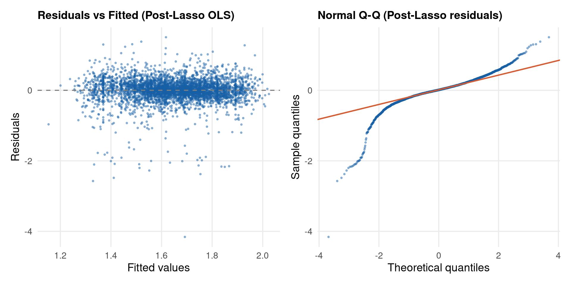
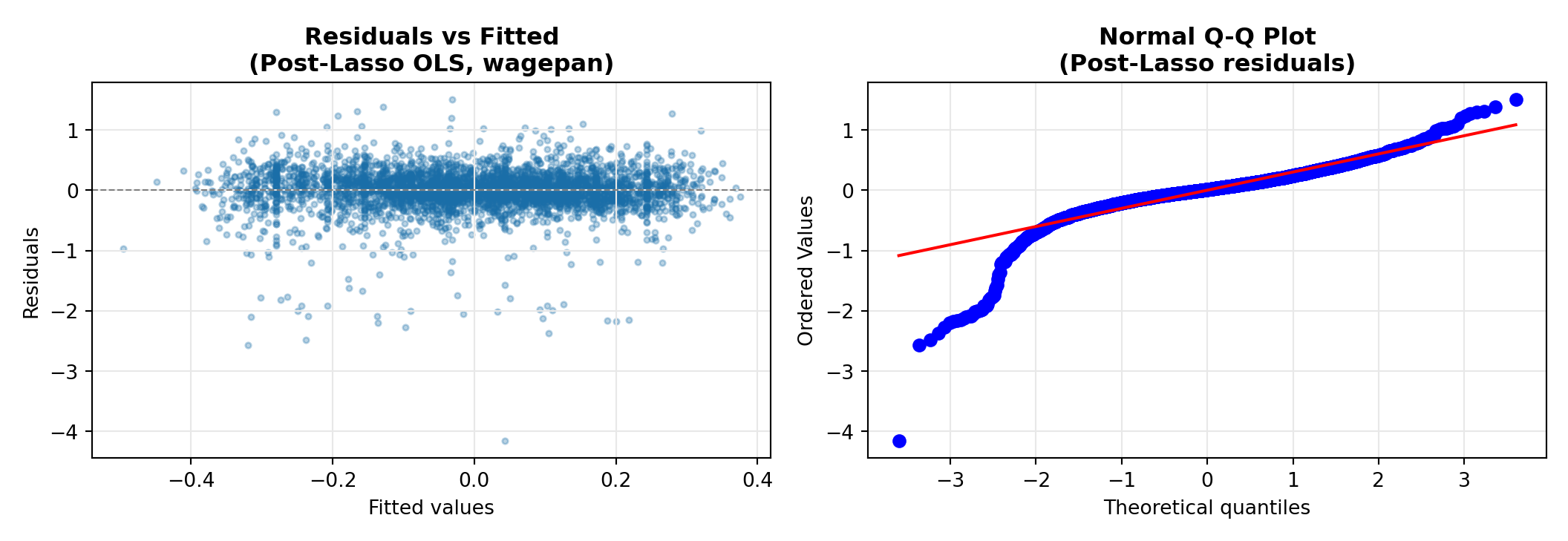
Breusch-Pagan (heteroskedasticity): χ²(df=11) = 28.7142  p = 0.0025

cat(sprintf("  → %s\n",
            if(bp_test$p.value < 0.05) "REJECT H0: heteroskedastic residuals → use HC3 SEs (already applied)"
            else "FAIL TO REJECT H0: residuals approximately homoskedastic"))

  → REJECT H0: heteroskedastic residuals → use HC3 SEs (already applied)

# 2. Serial correlation: Durbin-Watson
dw_test <- lmtest::dwtest(post_wp)
cat(sprintf("Durbin-Watson (serial corr.): DW = %.4f  p = %.4f\n",
            dw_test$statistic, dw_test$p.value))

Durbin-Watson (serial corr.): DW = 1.9221  p = 0.6005

# 3. RESET test: functional form
reset_test <- lmtest::resettest(post_wp, power = 2:3)
cat(sprintf("RESET (functional form): F(%d,%d) = %.4f  p = %.4f\n",
            reset_test$parameter[1], reset_test$parameter[2],
            reset_test$statistic, reset_test$p.value))

RESET (functional form): F(2,4345) = 5.6818  p = 0.0034

cat(sprintf("  → %s\n",
            if(reset_test$p.value < 0.05)
              "REJECT H0: non-linear terms significant → model may be misspecified"
            else "FAIL TO REJECT H0: no evidence of functional form misspecification"))

  → REJECT H0: non-linear terms significant → model may be misspecified

# 4. Residual diagnostic plots — ggplot
diag_df <- tibble(
  fitted   = fitted(post_wp),
  residual = resid_pl
)
p_rvf <- ggplot(diag_df, aes(fitted, residual)) +
  geom_point(colour = col_main, alpha = 0.4, size = 0.6) +
  geom_hline(yintercept = 0, linetype = "dashed", colour = "grey50") +
  labs(x = "Fitted values", y = "Residuals",
       title = "Residuals vs Fitted (Post-Lasso OLS)") +
  theme_lecture

# Q-Q via ggplot stat_qq
p_qq <- ggplot(diag_df, aes(sample = residual)) +
  stat_qq(colour = col_main, alpha = 0.4, size = 0.6) +
  stat_qq_line(colour = col_accent, linewidth = 0.8) +
  labs(x = "Theoretical quantiles", y = "Sample quantiles",
       title = "Normal Q-Q (Post-Lasso residuals)") +
  theme_lecture

p_rvf + p_qq    # patchwork side-by-side

import numpy as np, matplotlib.pyplot as plt
from scipy import stats

resid_py = y_py - X_full @ b_post_py
fitted_py = X_full @ b_post_py

# 1. Breusch-Pagan (manual)
from sklearn.linear_model import LinearRegression as LR
bp_ols = LR().fit(X_full, resid_py**2)
bp_r2  = 1 - np.sum((resid_py**2 - bp_ols.predict(X_full))**2) / \
             np.sum((resid_py**2 - np.mean(resid_py**2))**2)
bp_stat = len(y_py) * bp_r2
bp_df   = X_full.shape[1] - 1
bp_p    = 1 - stats.chi2.cdf(bp_stat, bp_df)
print(f"Breusch-Pagan: χ²({bp_df}) = {bp_stat:.4f}  p = {bp_p:.4f}")

Breusch-Pagan: χ²(12) = 28.7142  p = 0.0043

print(f"  → {'Heteroskedastic → use HC3 SEs (applied)' if bp_p<0.05 else 'Homoskedastic'}")

  → Heteroskedastic → use HC3 SEs (applied)

# 2. Normality of residuals
_, sw_p = stats.shapiro(resid_py[:5000] if len(resid_py)>5000 else resid_py)
print(f"Shapiro-Wilk: W = ...  p = {sw_p:.4f}")

Shapiro-Wilk: W = ...  p = 0.0000

# 3. Diagnostic plots
fig, axes = plt.subplots(1, 2, figsize=(11, 3.8))

ax = axes[0]
_ = ax.scatter(fitted_py, resid_py, alpha=0.3, s=8, color="#1a6ea8")
_ = ax.axhline(0, color="grey", lw=0.8, ls="--")
_ = ax.set_xlabel("Fitted values"); ax.set_ylabel("Residuals")
_ = ax.set_title("Residuals vs Fitted\n(Post-Lasso OLS, wagepan)", fontweight="bold")
_ = ax.grid(True, color="#e8e8e8")

ax2 = axes[1]
_ = stats.probplot(resid_py, plot=ax2)
_ = ax2.set_title("Normal Q-Q Plot\n(Post-Lasso residuals)", fontweight="bold")
_ = ax2.grid(True, color="#e8e8e8")

fig.tight_layout(); plt.show()

* Self-contained: reload wagepan, build the candidate control list.
frause wagepan, clear
xtset nr year

global ctrl "exper expersq married educ black hisp south"

* Post-selection OLS via the partialing-out lasso, then run the model
* diagnostics on a STANDARD regression (predict after `lasso` does not allow
* residuals — diagnostics need an estimation command that does).
quietly poregress lwage union, controls($ctrl i.year) rseed(14159)

* For residual-based diagnostics, refit the selected specification with regress.
* (Here we use the full hand-picked TWFE controls as a transparent stand-in so
*  estat/rvfplot have a standard linear model to work on.)
quietly regress lwage union exper expersq married educ i.year
predict resid_pds, residuals
predict yhat_pds,  xb

* 1. Heteroskedasticity: Breusch-Pagan
estat hettest
* H0: homoskedastic; rejection → use robust/HC SEs

* 2. Skewness-kurtosis normality test of residuals
sktest resid_pds
* H0: normally distributed residuals (large-n violations are informative)

* 3. Residual vs fitted plot
rvfplot, yline(0) title("Residuals vs Fitted — selected model")
quietly graph export "../plots/lasso_wp_rvf.png", replace width(1050) height(680)

Panel variable: nr (strongly balanced)
 Time variable: year, 1980 to 1987
         Delta: 1 unit







Breusch–Pagan/Cook–Weisberg test for heteroskedasticity 
Assumption: Normal error terms
Variable: Fitted values of lwage

H0: Constant variance

    chi2(1) =  13.44
Prob > chi2 = 0.0002


Skewness and kurtosis tests for normality
                                                         ----- Joint test -----
    Variable |       Obs   Pr(skewness)   Pr(kurtosis)   Adj chi2(2)  Prob>chi2
-------------+-----------------------------------------------------------------
   resid_pds |     4,360         0.0000         0.0000       1008.80     0.0000

Lasso — Extension: Deterrence and Crime (crime4)

A second panel application, on different terrain. crime4 is the Cornwell–Trumbull panel of 90 North Carolina counties, 1981–1987. The focal question is a deterrence elasticity: how does the (log) probability of arrest, lprbarr, move the (log) crime rate, lcrmrte, once we control for the many confounders an economist would worry about — other deterrence margins, demographics, sector wages, region? With county + year fixed effects and 20+ candidate controls, this is the same high-dimensional control selection problem as the union premium, so post-double-selection (PDS) Lasso transfers directly.

Warning

As with the union premium, Lasso selects the controls, not the causal design. prbarr is plausibly simultaneous with crime (more crime → strained enforcement → lower arrest rates), so read the estimate as the conditional association PDS delivers, not a settled causal elasticity.

• R
• Python
• Stata

cr <- crime4

cr$lcrmrte <- log(cr$crmrte)
cr$lprbarr <- log(cr$prbarr)
cr$lpolpc  <- log(cr$polpc)

focal     <- "lprbarr"
ctrl_vars <- c("prbconv", "prbpris", "avgsen", "lpolpc", "density", "taxpc",
               "pctmin80", "pctymle", "west", "central", "urban",
               "wcon", "wtuc", "wtrd", "wfir", "wser", "wmfg", "wfed", "wsta", "wloc")
ctrl_vars <- intersect(ctrl_vars, names(cr))

keep <- c("county", "year", "lcrmrte", focal, ctrl_vars)
cr   <- cr[complete.cases(cr[, keep]), keep]

# Two-way FE = within-county demean + year dummies
cr_dm <- group_by(cr, county)
cr_dm <- mutate(cr_dm, across(where(is.numeric),
                ~ . - mean(.) + mean(cr[[cur_column()]])))
cr_dm <- ungroup(cr_dm)
yr_d  <- model.matrix(~ factor(year) - 1, data = cr_dm)[, -1]
Xc    <- cbind(as.matrix(cr_dm[, ctrl_vars]), yr_d)

# Post-double-selection: Lasso the outcome on controls, and the focal regressor
# on controls; keep the union of selected controls; then OLS.
library(glmnet)
cv_y <- cv.glmnet(Xc, cr_dm$lcrmrte, alpha = 1, nfolds = 10)
cv_d <- cv.glmnet(Xc, cr_dm[[focal]], alpha = 1, nfolds = 10)
sel  <- union(which(coef(cv_y, s = "lambda.min")[-1] != 0),
              which(coef(cv_d, s = "lambda.min")[-1] != 0))

Xsel <- Xc[, sel, drop = FALSE]
pds  <- lm(cr_dm$lcrmrte ~ cr_dm[[focal]] + Xsel)
b    <- coef(pds)[2]
se   <- sqrt(sandwich::vcovHC(pds)[2, 2])
cat(sprintf("Controls selected (union): %d of %d\n", length(sel), ncol(Xc)))

Controls selected (union): 11 of 26

cat(sprintf("Deterrence elasticity (PDS Lasso): %.3f  (HC SE %.3f)\n", b, se))

Deterrence elasticity (PDS Lasso): -0.122  (HC SE 0.053)

import numpy as np
import pandas as pd
import wooldridge as woo
from sklearn.linear_model import LassoCV, LinearRegression

cr = woo.dataWoo("crime4").copy()
cr["lcrmrte"] = np.log(cr["crmrte"])
cr["lprbarr"] = np.log(cr["prbarr"])
cr["lpolpc"]  = np.log(cr["polpc"])

focal = "lprbarr"
ctrl  = [c for c in ["prbconv", "prbpris", "avgsen", "lpolpc", "density", "taxpc",
                     "pctmin80", "pctymle", "west", "central", "urban",
                     "wcon", "wtuc", "wtrd", "wfir", "wser", "wmfg",
                     "wfed", "wsta", "wloc"] if c in cr.columns]
cr = cr.dropna(subset=["lcrmrte", focal] + ctrl)

# Two-way FE: within-county demean + year dummies
num = ["lcrmrte", focal] + ctrl
cr[num] = cr.groupby("county")[num].transform(lambda v: v - v.mean()) + cr[num].mean()
yr = pd.get_dummies(cr["year"], drop_first=True).astype(float).to_numpy()
Xc = np.column_stack([cr[ctrl].to_numpy(float), yr])

cv_y = LassoCV(cv=10).fit(Xc, cr["lcrmrte"].to_numpy())
cv_d = LassoCV(cv=10).fit(Xc, cr[focal].to_numpy())
sel  = np.where((cv_y.coef_ != 0) | (cv_d.coef_ != 0))[0]

Xpds = np.column_stack([cr[focal].to_numpy(), Xc[:, sel]])
pds  = LinearRegression().fit(Xpds, cr["lcrmrte"].to_numpy())
print(f"Controls selected (union): {len(sel)} of {Xc.shape[1]}")

Controls selected (union): 18 of 26

print(f"Deterrence elasticity (PDS Lasso): {pds.coef_[0]:.3f}")

Deterrence elasticity (PDS Lasso): -0.124

* frause loads the Wooldridge datasets directly (no CSV export needed)
frause crime4, clear
xtset county year
gen lcrmrte = log(crmrte)
gen lprbarr = log(prbarr)
gen lpolpc  = log(polpc)

* Post-double-selection inference for the deterrence elasticity.
* i.year handles year FE; county FE via within-demean or by absorbing.
dsregress lcrmrte lprbarr, ///
    controls(prbconv prbpris avgsen lpolpc density taxpc ///
             pctmin80 pctymle west central urban ///
             wcon wtuc wtrd wfir wser wmfg wfed wsta wloc i.year)

Lasso — Part Summary: Take-Home Notes

• Lasso
• Connections
• Report
• Mistakes

What Lasso does:

• Solves \(\min_\beta \|\mathbf{y}-\mathbf{X}\beta\|^2 + \lambda\|\beta\|_1\)
• Sets small coefficients to exactly zero (variable selection)
• Shrinks non-zero coefficients toward zero (shrinkage bias)
• CV selects \(\hat\lambda\) — two choices: lambda.min (predict) vs lambda.1se (infer)

Connection to economics:

• Lasso = automatic control selection for Mincer/TWFE equations
• PDS-Lasso = valid causal inference after Lasso selection
• Adaptive Lasso = oracle property (correct selection probability → 1)
• Sparsity assumption: most of your candidate controls are noise

What you report:

• Always post-Lasso OLS \(\tilde\beta^{post}\), not \(\hat\beta^{lasso}\)
• The selected set \(\hat{\mathcal{S}}\) and its size
• The \(\hat\lambda\) and selection method
• Test the post-Lasso OLS model (BP, RESET, serial correlation)

Common mistakes:

• Reporting \(\hat\beta^{lasso}\) as a causal effect
• Using lambda.min when inference is the goal
• Forgetting to standardise (scale non-equivariance)
• Interpreting \(\hat\beta_j = 0\) as “no effect”

Lasso — Progress from TWFE · What Still Lacks

• Progress over TWFE
• Still lacking

• ✓ Automatic control selection — no researcher degrees of freedom in choosing \(\mathbf{x}_{it}\)
• ✓ Works when \(p > n_{\text{eff}}\) — OLS/TWFE undefined; Lasso always has a unique solution
• ✓ Reduces over-control bias — dropping noise controls improves efficiency
• ✓ Reproducible — the selection rule is transparent and algorithmic
• ✓ Foundation for causal ML — PDS-Lasso enables valid IV and DML

• ✗ No valid inference on \(\hat\beta_j^{lasso}\) — post-selection distribution is non-normal; confidence intervals from Lasso are invalid
• ✗ Instability with correlated controls — Lasso picks one from a correlated group arbitrarily
• ✗ Sparsity assumption required — fails in dense-signal settings (→ Ridge, Elastic Net)
• ✗ Not causal by itself — Lasso \(\hat\beta^{union}\) is not the causal effect without PDS correction
• ✗ Fixed effects remain ad hoc — Lasso selects time-varying controls but FE elimination is still by assumption

Lasso — Bibliography

Foundational:

• Tibshirani (1996). Lasso. doi:10.1111/j.2517-6161.1996.tb02080.x
• Zou (2006). Adaptive Lasso. doi:10.1198/016214506000000735
• Belloni, Chernozhukov & Hansen (2014). High-dimensional methods in economics. doi:10.1257/jep.28.2.29

Theoretical:

• Leeb & Pötscher (2005). Model selection and inference. doi:10.1017/S0266466605050036
• Fan & Li (2001). Variable selection via nonconcave penalised likelihood. doi:10.1198/016214501753382273
• Belloni & Chernozhukov (2011). High-dimensional sparse econometric models. doi:10.1007/978-3-642-19811-7_3
• Bickel, Ritov & Tsybakov (2009). Simultaneous analysis of Lasso and Dantzig selector. doi:10.1214/08-AOS620

Approximate sparsity (the econometric foundation):

• Belloni, Chernozhukov & Hansen (2013). Inference on treatment effects after selection among high-dimensional controls. doi:10.1093/restud/rdt044
• Belloni, Chernozhukov & Hansen (2012). Sparse models and methods for optimal instruments. doi:10.1093/restud/rds044

Econometric applications:

• Mincer (1974). Schooling, Experience and Earnings. NBER.

Textbook chapters:

• Hansen (2022). Econometrics. Princeton University Press — Ch. 29 (Machine Learning), §29.8–29.14 (Lasso, approximate sparsity)
• ISLR §6.1–6.2 (James, Witten, Hastie & Tibshirani 2023)
• Wooldridge (2010) Econometric Analysis of Cross Section and Panel Data §20

Lasso — Exercises

1. Variable selection stability — run Lasso on wagepan with three \(\lambda\) choices: lambda.min, lambda.1se, and the plugin \(\lambda\) from hdm::rlasso. How many variables does each select? Which appear in all three? What does the overlap tell you?

2. Post-Lasso validity — after fitting Post-Lasso OLS on wagepan, run the Breusch–Pagan and RESET tests. If you reject RESET, what does that imply about the linear Mincer specification? How would you address it?

3. Comparison with TWFE — compare the Post-Lasso OLS union premium to the TWFE estimate. Are they statistically different at the 5% level? If so, what omitted controls might explain the gap?

4. Adaptive Lasso — on wagepan, compare CV Lasso with Adaptive Lasso (selection(adaptive) in Stata; penalty-factor reweighting 1/|β̂| in glmnet). Does the adaptive version select fewer controls? Does the union premium move?

5. Bias–variance in reporting — on wagepan, compute the Lasso union premium at 20 values of \(\lambda\) from lambda.max to lambda.min. Plot the estimate and its 95% CI (post-Lasso OLS at each \(\lambda\)) against \(\log(\lambda)\). Describe the trade-off.

6. Convergence diagnostics — refit the wagepan Lasso with thresh = 1e-3 then thresh = 1e-9 (R) / tol in scikit-learn. How do the selected set and runtime change? Now turn standardisation off on raw-scale controls — what happens to convergence, and why?

7. Coordinate descent by hand — extend the from-scratch lasso_cd to Elastic Net (add the \(1+\lambda(1-\alpha)\) denominator and threshold at \(\lambda\alpha\)). Verify against glmnet at \(\alpha = 0.5\) on the wagepan controls.

8. Extension — crime4 deterrence — reproduce the PDS-Lasso deterrence elasticity (lprbarr → lcrmrte) with county + year FE. Now add polpc (police per capita) as a second focal regressor and double-select for both. How sensitive is the arrest-probability coefficient to including police?

9. Extension — card returns to schooling — on card (cross-section), estimate the return to educ on lwage using PDS-Lasso over the regional dummies (reg661–reg669), parental education, black, smsa, and family-structure controls. Compare the Lasso-selected OLS return with the naïve all-controls OLS. Which controls survive selection?

10. card instrument check — nearc4 (grew up near a 4-year college) is the classic instrument for educ. Lasso-select controls for both the first stage (educ on nearc4 + controls) and the reduced form. Does double-selection change which controls you would include in a 2SLS specification?

Lasso — Full Code

Complete, standalone scripts for this part — libraries loaded and configuration hard-coded, so each file runs on its own. Download the language you want:

R

⬇ Download lasso.R

Python

⬇ Download lasso.py

Stata

⬇ Download lasso.do

All code shown live on the step slides; these files bundle it for re-use.

Part III — Ridge

“Why throw away a variable? Why not just make it smaller?”

Lasso bet on sparsity. But in wagepan, education, experience, occupation,
industry — they all matter, just in different amounts.
Ridge keeps them all. It just makes the small ones whisper.

Ridge — Econometric Framework

From Lasso to Ridge: Lasso selected a sparse model. But if the true wage equation has many small effects — occupation cells, regional variations, industry cycles — zeroing them out introduces bias. Ridge says: keep everything, shrink proportionally.

The Ridge wage equation:

\[\hat{\boldsymbol\gamma}^R = \arg\min_{\boldsymbol\gamma} \|\mathbf{y} - D\beta - \mathbf{X}\boldsymbol\gamma\|_2^2 + \lambda\|\boldsymbol\gamma\|_2^2\]

All \(p\) controls enter with shrinkage factor \(d_j^2/(d_j^2 + \lambda)\) per principal component direction \(d_j\). Controls with small variance contribution (collinear, redundant) are shrunk more.

Connection to econometrics:

Ridge is the MAP estimator under Gaussian priors \(\beta_j \sim \mathcal{N}(0, \sigma^2/\lambda)\). In the wage context: we believe a priori that no single control should dominate, and that small effects exist everywhere.

On wagepan: Ridge will keep all industry × occupation dummies active, each contributing a small amount. Compare to Lasso which dropped most of them. The question is: does the union premium estimate change?

Regularised Regression — Ridge: Motivation

• ① When OLS breaks down
• ② What we lose without Ridge
• ③ Callouts

Three situations where OLS fails and Ridge provides a solution:

1. Multicollinearity — \(\mathbf{X}^\top\mathbf{X}\) is ill-conditioned. The condition number \(\kappa = d_{\max}/d_{\min} \gg 1\) means \((\mathbf{X}^\top\mathbf{X})^{-1}\) amplifies estimation noise. Tiny perturbations in the data produce enormous swings in \(\hat{\boldsymbol\beta}^{\text{OLS}}\): standard errors explode, signs flip across bootstrap samples. Econometric examples: distributed lag models, gravity equations with many bilateral controls, input-output tables, factor models with correlated factors.
2. More predictors than observations (\(p \geq n\)). \(\mathbf{X}^\top\mathbf{X}\) is rank-deficient — singular. OLS has no unique solution; infinitely many \(\hat{\boldsymbol\beta}\) fit the training data perfectly but fail catastrophically out-of-sample. Econometric examples: policy evaluation with rich survey controls, text-as-data regressions, high-dimensional demand systems.
3. Dense signal — many small, real effects. If all \(p\) predictors matter at small magnitudes, Lasso discards real signal by zeroing coefficients. Ridge shrinks all gently and preserves the full signal structure. Econometric examples: wage equations with occupation-industry-region cells, macro forecasting with many correlated indicators, retail price transmission across many outlets.

Problem	Without Ridge	With Ridge
Collinear predictors	SE explodes, signs unstable	Stable estimates, reduced SE
\(p \approx n\)	Overfits, poor OOS performance	Regularised, generalises well
\(p > n\)	No unique solution	Always a unique solution
Dense signal	Lasso zeroes real predictors	Keeps all, shrinks proportionally
Numerical stability	Near-singular inversion fails	\(+\lambda\mathbf{I}\) guarantees PD matrix

What Ridge does: adds \(\lambda \mathbf{I}_p\) to the Gram matrix before inverting:

\[\hat{\boldsymbol\beta}^{\text{ridge}} = \underbrace{(\mathbf{X}^\top\mathbf{X} + \lambda \mathbf{I}_p)}_{\text{always invertible, } \lambda > 0}{}^{-1}\mathbf{X}^\top\mathbf{y}\]

The cost: every \(\hat\beta_j^{\text{ridge}}\) is biased toward zero by \(\frac{d_j^2}{d_j^2+\lambda}\) per principal direction. Acceptable for prediction; must be corrected for causal inference (via DML).

⚠️  Ridge Does Not Perform Variable Selection

All \(p\) coefficients remain strictly non-zero at any \(\lambda > 0\). Ridge shrinks every coefficient toward zero but never exactly to zero.

If sparsity is the goal — a few large effects, many true zeros — Ridge is the wrong method:

• Use Lasso when predictors are independent and DGP is sparse
• Use Elastic Net when predictors are correlated and DGP is sparse

Geometric reason: the \(\ell_2\) constraint set is a smooth sphere — the OLS loss ellipsoid touches it on its curved surface, never at a corner on an axis. Only corners produce exact zeros.

📝  Bayesian Interpretation of Ridge

Ridge is the MAP (maximum a posteriori) estimator under independent Gaussian priors:

\[\beta_j \overset{\text{iid}}{\sim} \mathcal{N}\!\left(0,\, \frac{\sigma^2}{\lambda}\right)\]

\(\lambda\) encodes prior belief that coefficients are small. Larger \(\lambda\) → stronger prior → stronger shrinkage toward zero.

Prior-penalty correspondence:

• Gaussian prior \(\mathcal{N}(0,\sigma^2/\lambda)\) → Ridge (\(\ell_2\) penalty)
• Laplace prior \(\text{Laplace}(0, 1/\lambda)\) → Lasso (\(\ell_1\) penalty)
• Spike-and-slab prior → subset selection (hard thresholding)

💡  Ridge Bias–Variance Trade-off

\[\text{MSE}(\hat{\boldsymbol\beta}^{\text{ridge}}) = \underbrace{\text{Bias}^2}_{\propto\,\lambda^2} + \underbrace{\text{Var}}_{\propto\,1/\lambda}\]

Ridge deliberately introduces bias to sharply reduce variance. The MSE is U-shaped in \(\lambda\):

• \(\lambda \to 0\): OLS — zero bias, high variance
• \(\lambda \to \infty\): zero coefficients — maximum bias, zero variance
• \(\lambda^*\) (interior): minimises total MSE — found by CV

Hoerl & Kennard (1970): there always exists a \(\lambda^* > 0\) such that \(\text{MSE}(\hat{\boldsymbol\beta}^{\text{ridge}}) < \text{MSE}(\hat{\boldsymbol\beta}^{\text{OLS}})\).

Regularised Regression — Ridge: Mathematics I

Primal problem (penalised least squares):

\[\hat{\boldsymbol\beta}^{\text{ridge}} = \arg\min_{\boldsymbol\beta} \underbrace{\|\mathbf{y} - \mathbf{X}\boldsymbol\beta\|_2^2}_{\text{fit}} + \lambda\underbrace{\|\boldsymbol\beta\|_2^2}_{\text{penalty}} \qquad \lambda \geq 0\]

Closed-form solution — first-order condition \(-2\mathbf{X}^\top(\mathbf{y}-\mathbf{X}\boldsymbol\beta) + 2\lambda\boldsymbol\beta = 0\):

\[\boxed{\hat{\boldsymbol\beta}^{\text{ridge}} = (\mathbf{X}^\top\mathbf{X} + \lambda \mathbf{I}_p)^{-1}\mathbf{X}^\top\mathbf{y}}\]

Equivalent constrained form (Lagrangian duality):

\[\hat{\boldsymbol\beta}^{\text{ridge}} = \arg\min_{\boldsymbol\beta} \|\mathbf{y}-\mathbf{X}\boldsymbol\beta\|_2^2 \quad \text{s.t.} \quad \|\boldsymbol\beta\|_2^2 \leq t(\lambda)\]

The \(\ell_2\) constraint set is a sphere — the OLS ellipsoid touches the sphere on its curved surface, never at a corner. This is the geometric reason Ridge never produces exact zeros.

Key properties:

Property	Result
Unique solution?	Always, for any \(\lambda > 0\)
Exact zeros (sparsity)?	Never
Scale-invariant?	No — always standardise \(\mathbf{X}\) first
Consistent as \(n \to \infty\)?	Yes, provided \(\lambda/n \to 0\)
\(\lambda\) selection	10-fold CV (standard) or GCV (closed form)
Computational cost	\(\mathcal{O}(p^3)\) — one matrix inversion

💡  Generalised Cross-Validation (GCV)

Closed-form leave-one-out approximation — no refitting required:

\[\text{GCV}(\lambda) = \frac{\|\mathbf{y}-\hat{\mathbf{y}}(\lambda)\|^2/n}{\bigl[1-\text{df}(\lambda)/n\bigr]^2}\]

where \(\text{df}(\lambda) = \sum_j d_j^2/(d_j^2+\lambda)\) are the effective degrees of freedom.

Preferred over \(K\)-fold CV when \(n\) is very large or the \(\lambda\) grid is dense — GCV scales as \(\mathcal{O}(np)\) rather than \(\mathcal{O}(Knp)\).

⚠️  Ridge is NOT Scale-Invariant

OLS: multiplying \(X_j\) by \(c\) simply rescales \(\hat\beta_j\) by \(1/c\) — the prediction \(X_j\hat\beta_j\) is unchanged. This is called scale equivariance.

Ridge: the \(\ell_2\) penalty treats all coefficients as equally important. A coefficient on income in dollars will be penalised 1000× harder than the same coefficient expressed in thousands of dollars.

The formula: standardise each predictor to unit variance before fitting, then report coefficients on the original scale:

\[\tilde{x}_{ij} = x_{ij}/\hat\sigma_j\]

After fitting on standardised data, the coefficient for \(X_j\) on the original scale is \(\hat\beta_j^{\text{ridge}}/\hat\sigma_j\).

ISLR §6.2.1, p. 239 — James, Witten, Hastie & Tibshirani (2023)

Regularised Regression — Ridge: Mathematics II

SVD representation — the most transparent form of Ridge

Let \(\mathbf{X} = \mathbf{U}\mathbf{D}\mathbf{V}^\top\) (thin SVD), singular values \(d_1 \geq \cdots \geq d_p > 0\):

\[\hat{\boldsymbol\beta}^{\text{ridge}} = \sum_{j=1}^p \underbrace{\frac{d_j^2}{d_j^2 + \lambda}}_{\text{shrinkage factor} \in (0,1)} \cdot \underbrace{\frac{\mathbf{u}_j^\top\mathbf{y}}{d_j}}_{\text{OLS component}} \cdot \mathbf{v}_j\]

Direction-by-direction reading:

• Large \(d_j\) (high-variance direction): shrinkage factor \(\approx 1\) → barely shrunk
• Small \(d_j\) (near-collinear direction): shrinkage factor \(\approx 0\) → aggressively shrunk

Ridge is direction-dependent shrinkage — it respects the geometry of \(\mathbf{X}\).

Effective degrees of freedom:

\[\text{df}(\lambda) = \sum_{j=1}^p \frac{d_j^2}{d_j^2+\lambda} \;\in\; (0,\, p)\]

Analytical bias and variance (over repeated samples, fixed \(\mathbf{X}\)):

\[\text{Bias}^2 = \lambda^2 \sum_{j=1}^p \frac{(\mathbf{v}_j^\top\boldsymbol\beta^*)^2}{(d_j^2+\lambda)^2}, \qquad \text{Var} = \sigma^2 \sum_{j=1}^p \frac{d_j^2}{(d_j^2+\lambda)^2}\]

MSE = Bias² + Var is U-shaped in \(\lambda\) — there exists an optimal interior \(\lambda^* > 0\).

📝  Hoerl & Kennard (1970) — Optimal \(\lambda\)

The MSE-minimising ridge penalty has the closed form:

\[\lambda^* = \frac{p\sigma^2}{\|\boldsymbol\beta^*\|^2}\]

Since both \(\sigma^2\) and \(\boldsymbol\beta^*\) are unknown, this formula cannot be used directly. Cross-validation estimates \(\lambda^*\) from the data.

Reference: Hoerl & Kennard (1970). doi:10.1080/00401706.1970.10488634

Ridge — When It Excels and When It Fails

• ✓ Use Ridge when
• ✗ Do NOT use Ridge when

1. Collinear predictors — Macro time series (lags, rates, indices), input-output tables, multi-wave panels — Ridge is robust; OLS SEs explode and signs flip arbitrarily.

2. Dense signal — most predictors contribute real but small effects. Factor models, spectral data, demand systems with many substitutes. Lasso discards genuine signal; Ridge retains it all.

3. \(p\) close to or exceeding \(n\) — Ridge always produces a unique solution. Even \(p/n = 0.5\) is enough for OLS to overfit severely.

4. Nuisance estimation in DML/IV — When you need low-MSE predictions of \(g(\mathbf{x}) = \mathbb{E}[y|\mathbf{X}]\) for a second stage — Ridge is ideal because all that matters is predictive accuracy, not sparsity.

5. Distributed lag models — Lags are highly collinear by construction. Ridge stabilises the entire lag profile without zeroing out economically meaningful lags.

6. Computational convenience — Closed-form solution: \(\mathcal{O}(p^3)\) per \(\lambda\). Faster than Lasso’s iterative coordinate descent for very large \(p\).

💡  Ridge Regularisation is Everywhere

Method	Connection to Ridge
XGBoost lambda	\(\ell_2\) penalty on leaf weights — Ridge on tree outputs
Principal Component Regression (PCR)	Drops small-\(d_j\) directions = Ridge with hard threshold
Neural network weight decay	\(\ell_2\) penalty on weights = Ridge per layer
Bayesian MAP (Gaussian prior)	\(\beta_j \sim \mathcal{N}(0,\sigma^2/\lambda)\) → Ridge posterior mode

1. You need variable selection — Ridge never sets any \(\hat\beta_j\) to exactly zero. All \(p\) predictors remain. Use Lasso or Elastic Net for sparse models.

2. You want valid inference on individual \(\hat\beta_j\) — Ridge coefficients are biased. OLS standard errors are wrong after regularisation. Do not report \(t\)-statistics or \(p\)-values from a Ridge fit. Use post-double-selection (PDS-Lasso) or DML for causal inference.

3. The true DGP is sparse — A few large signals, many true zeros. Ridge spreads shrinkage evenly and performs worse than Lasso. Compare via CV before committing.

4. \(n \gg p\), no collinearity — OLS is already BLUE. Ridge adds bias with no variance benefit — it strictly worsens performance.

5. Many-level categorical predictors — Ridge treats all dummy levels symmetrically. Group Lasso or hierarchical priors are more appropriate.

⚠️  The Fundamental Cost of Ridge

Every \(\hat\beta_j^{\text{ridge}}\) is biased toward zero by \(d_j^2/(d_j^2+\lambda)\) per PC direction.

For prediction: this bias is acceptable — it reduces variance and improves OOS MSE.

For causal inference: reporting Ridge coefficients as treatment effect estimates is invalid. Use one of:

• DML (Chernozhukov et al. 2018) — Ridge as nuisance estimator, OLS for the treatment parameter
• Post-double-selection — Lasso selects controls, then unpenalised IV/OLS

Ridge — The Setup

Data: wagepan (Wooldridge) — 545 men, 1980–1987, \(N = 4{,}360\) person-year observations. Ridge predicts log wage from a deliberately collinear, high-dimensional control block (experience polynomial, education, demographics, and many industry / occupation / region dummies, \(p = 33\)). The standardised control matrix is near-singular (\(\kappa(\mathbf{X}^\top\mathbf{X})\) enormous) — exactly the regime where OLS is unstable and Ridge earns its place.

Each step is shown in R, Python, and Stata so results can be replicated in any environment.

📝  Stata Ridge Toolbox (since Stata 16)

Ridge = elasticnet linear y varlist, alpha(0)  (pure \(\ell_2\) penalty).

Command	Purpose
splitsample	70/30 train/test split (firewall principle)
lassogof	MSE and R² by sample (train vs test)
cvplot	CV error path — shows U-shaped bias-variance trade-off
coefpath	Ridge coefficient trace — smooth shrinkage to zero
lassoinfo	CV-selected \(\lambda\), effective df, non-zero count
lassocoef	Penalised coefficients at selected \(\lambda\)

Ridge — Key Functions: Fitting

The fitting call in each language, annotated argument by argument. Ridge differs from Lasso only in the mixing parameter (alpha = 0 / l1_ratio = 0); cross-validation and extraction follow on the next slide.

• R — glmnet
• Python — scikit-learn
• Stata — elasticnet

fit <- glmnet(
  X,                              # numeric MATRIX (n × p), NOT a data.frame
  y,                              # response vector, length n
  family      = "gaussian",       # "gaussian" for linear regression (optional)
  alpha       = 0,                # 0 = Ridge (ℓ₂); 1 = Lasso; (0,1) = Elastic Net
  lambda      = NULL,             # NULL → glmnet auto-computes the λ path
  nlambda     = 100,              # number of λ values on that path (default 100)
  standardize = TRUE              # scale X to unit SD before penalising (mandatory)
)
# fit$beta → p × nlambda coefficient matrix — for Ridge, NONE are ever exactly 0
# Closed form: β̂(λ) = (XᵀX + λI)⁻¹ Xᵀy, solved efficiently via the SVD

Math connection: Ridge has a closed form, \(\hat{\boldsymbol\beta}(\lambda)=(\mathbf{X}^\top\mathbf{X}+\lambda\mathbf{I})^{-1}\mathbf{X}^\top\mathbf{y}\); per principal-component direction the OLS estimate is shrunk by \(d_j^2/(d_j^2+\lambda)\), and the effective df is \(\sum_j d_j^2/(d_j^2+\lambda)\).

from sklearn.linear_model import Ridge

fit = Ridge(
    alpha        = 1.0,       # the single λ (ℓ₂ penalty strength); NOT cross-validated here
    fit_intercept= True,      # estimate an unpenalised intercept (default True)
    solver       = "auto"     # "cholesky"/"svd" direct solvers; "auto" picks one
)
fit.fit(X, y)                 # X: numpy array (n × p); y: numpy array (n,)
# fit.coef_      → coefficient array length p (all non-zero — Ridge never zeroes)
# fit.intercept_ → fitted intercept
# NOTE: Ridge does NOT standardise — wrap StandardScaler in a Pipeline

Math connection: a single alpha \(=\lambda\); Ridge uses a direct linear solver (Cholesky/SVD), not coordinate descent, because the \(\ell_2\) problem is smooth.

elasticnet linear lwage $ctrl,   ///
    alpha(0)                     /// 0 = Ridge (ℓ₂); 1 = Lasso; (0,1) = Elastic Net
    grid(100)                    /// number of λ values on the path (default 100)
    nolog                        // suppress the iteration log
* Stata standardises covariates internally and back-transforms.

Math connection: alpha(0) selects the pure \(\ell_2\) penalty; with no \(\ell_1\) term there is no variable selection — every coefficient stays non-zero at every \(\lambda\).

Ridge — Key Functions: Cross-Validation & Extraction

Cross-validation picks \(\lambda\); then you extract coefficients and predictions. For Ridge the selected model always retains all \(p\) predictors.

• R — glmnet
• Python — scikit-learn
• Stata — elasticnet

cv_ridge <- cv.glmnet(
  X,                              # same matrix as the fit
  y,                              # same response vector
  alpha        = 0,               # 0 = Ridge (match the fit)
  nfolds       = 10,              # number of CV folds (default 10)
  type.measure = "mse"            # select λ by out-of-fold mean squared error
)
# cv_ridge$lambda.min → λ minimising CV-MSE
# cv_ridge$lambda.1se → largest λ within 1 SE (more shrinkage, simpler model)

# Extract coefficients at the chosen λ (all p are non-zero):
b_ridge <- coef(cv_ridge, s = "lambda.min")[-1]
cat(sum(b_ridge != 0), "non-zero out of", length(b_ridge))  # always p

# Predict on new data:
yhat <- predict(cv_ridge, newx = X_test, s = "lambda.min")

Math connection: the CV-MSE curve is U-shaped in \(\lambda\); lambda.min sits at its trough.

from sklearn.linear_model import RidgeCV
from sklearn.preprocessing import StandardScaler
from sklearn.pipeline import Pipeline
import numpy as np

# RidgeCV fits the path AND cross-validates λ; a Pipeline enforces correct scaling:
pipe_ridge = Pipeline([
    ("scaler", StandardScaler()),       # fit on training data only, apply to test
    ("ridge",  RidgeCV(
        alphas = np.logspace(-2, 4, 100),  # the λ grid to search
        cv     = 10                        # number of CV folds
    ))
])
pipe_ridge.fit(X_train, y_train)
model = pipe_ridge.named_steps["ridge"]
# model.alpha_ → selected λ
# model.coef_  → all p non-zero (Ridge never zeroes)
y_hat = pipe_ridge.predict(X_test)        # pipeline scales internally

Why Pipeline? StandardScaler must be fitted on training data only, then applied to test — the pipeline enforces that order automatically, avoiding leakage.

elasticnet linear lwage $ctrl,   ///
    alpha(0)                     /// 0 = Ridge
    selection(cv, folds(10))     /// CV selects λ
    rseed(14159)                 /// reproducible fold assignment
    nolog                        // suppress iteration log

* Post-estimation (same commands as lasso):
lassoinfo                                 // λ*, no. of non-zero coefs (= p for Ridge)
lassocoef, display(coef, penalized)       // penalised Ridge coefficients
cvplot                                    // CV error U-shape
coefpath                                  // smooth shrinkage traces (no hard zeros)

Ridge vs Lasso in Stata: the only difference is alpha(0) vs alpha(1). coefpath shows smooth curves approaching zero (Ridge) rather than abrupt jumps to zero (Lasso).

Ridge — Step 1: Data and Split

• R
• Python
• Stata

library(wooldridge)

wp <- wagepan

# - Outcome and a deliberately collinear, high-dimensional control block
y_col   <- "lwage"
cand    <- c("exper", "expersq", "educ", "married", "union", "black", "hisp",
             "south", "nrthcen", "nrtheast", "rur",
             "agric", "bus", "construc", "ent", "fin", "manuf", "min",
             "pro", "pub", "tra", "trad",
             "occ1", "occ2", "occ3", "occ4", "occ5", "occ6", "occ7", "occ8", "occ9",
             "poorhlth", "hours")
cand    <- intersect(cand, names(wp))
dat     <- wp[stats::complete.cases(wp[, c(y_col, cand)]), c(y_col, cand)]

X_r <- as.matrix(dat[, cand])
y_r <- dat[[y_col]]
n   <- nrow(X_r)
p   <- ncol(X_r)

# Standardise BEFORE fitting — Ridge is scale-sensitive
X_s       <- scale(X_r)
kappa_val <- kappa(t(X_s) %*% X_s)
cat(sprintf("n = %d  |  p = %d controls\n", n, p))

n = 4360  |  p = 33 controls

cat(sprintf("κ(X'X) = %.0f  [>30 problematic, >1000 severe]\n", kappa_val))

κ(X'X) = 64504055000854576  [>30 problematic, >1000 severe]

# 70/30 train/test split (firewall principle: test set never used in fitting)
set.seed(SEED)
tr_idx <- sample(n, floor(0.7 * n))
te_idx <- setdiff(seq_len(n), tr_idx)
X_tr <- X_s[tr_idx, ]
y_tr <- y_r[tr_idx]
X_te <- X_s[te_idx, ]
y_te <- y_r[te_idx]
cat(sprintf("Train: %d  |  Test: %d\n", length(tr_idx), length(te_idx)))

Train: 3052  |  Test: 1308

import numpy as np
import pandas as pd
import wooldridge as woo
from sklearn.preprocessing import StandardScaler

# - Real data: wagepan. Ridge as prediction of log wage from collinear controls.
wp_py = woo.dataWoo("wagepan")
cand = [c for c in ["exper","expersq","educ","married","union","black","hisp",
                    "south","nrthcen","nrtheast","rur",
                    "agric","bus","construc","ent","fin","manuf","min",
                    "pro","pub","tra","trad",
                    "occ1","occ2","occ3","occ4","occ5","occ6","occ7","occ8","occ9",
                    "poorhlth","hours"]
        if c in wp_py.columns]
dat_py = wp_py[["lwage"] + cand].dropna()
X_py = dat_py[cand].to_numpy(dtype=float)
y_py = dat_py["lwage"].to_numpy()
n, p = X_py.shape

sc   = StandardScaler()
X_sc = sc.fit_transform(X_py)   # centre + scale to σ=1 per predictor
kappa_py = np.linalg.cond(X_sc.T @ X_sc)
print(f"n = {n}  |  p = {p} controls")

n = 4360  |  p = 33 controls

print(f"κ(X'X) = {kappa_py:.0f}  [>30 problematic, >1000 severe]")

κ(X'X) = 6392640504952890  [>30 problematic, >1000 severe]

# 70/30 split — same seed as R
rng2   = np.random.default_rng(SEED)
tr_idx = rng2.choice(n, size=int(0.7 * n), replace=False)
te_idx = np.setdiff1d(np.arange(n), tr_idx)
X_tr_py, X_te_py = X_sc[tr_idx], X_sc[te_idx]
y_tr_py, y_te_py = y_py[tr_idx], y_py[te_idx]
print(f"Train: {len(tr_idx)}  |  Test: {len(te_idx)}")

Train: 3052  |  Test: 1308

* Real data: wagepan via frause. Ridge as prediction of log wage from a
* collinear, high-dimensional control block. No simulation.
frause wagepan, clear

* Control block (those present in this copy of wagepan)
local ctrl exper expersq educ married union black hisp south ///
           nrthcen nrtheast rur agric bus construc ent fin manuf min ///
           pro pub tra trad occ1 occ2 occ3 occ4 occ5 occ6 occ7 occ8 occ9 ///
           poorhlth hours
global RCTRL `ctrl'

* Condition number of the standardised control matrix via Mata
mata:
    vl = tokens(st_local("ctrl"))
    X  = st_data(., vl)
    X  = (X :- mean(X)) :/ sqrt(diagonal(variance(X))')
    ev = Re(eigenvalues(X'X))
    printf("kappa(X'X) = %g  [>30 problematic; >1000 severe]\n", max(ev)/min(ev))
end

* 70/30 split — splitsample is the Stata built-in; rseed matches R/Python
splitsample, generate(sample) split(0.7 0.3) rseed(14159)
label define lbsample 1 "Training" 2 "Test"
label values sample lbsample
tabulate sample

------------------------------------------------- mata (type end to exit) ----------------------------------------------
:     vl = tokens(st_local("ctrl"))

:     X  = st_data(., vl)

:     X  = (X :- mean(X)) :/ sqrt(diagonal(variance(X))')

:     ev = Re(eigenvalues(X'X))

:     printf("kappa(X'X) = %g  [>30 problematic; >1000 severe]\n", max(ev)/min(ev))
kappa(X'X) = -1.9679e+14  [>30 problematic; >1000 severe]

: end
------------------------------------------------------------------------------------------------------------------------

     sample |      Freq.     Percent        Cum.
------------+-----------------------------------
   Training |      3,052       70.00       70.00
       Test |      1,308       30.00      100.00
------------+-----------------------------------
      Total |      4,360      100.00

Ridge — Step 2: Fit OLS and Ridge

• R
• Python
• Stata

# OLS — fitted on training sample; likely unstable due to high κ
ols_tr     <- lm(y_tr ~ X_tr)

# Ridge — 10-fold CV on training sample selects λ
# alpha = 0 → pure L2 penalty (Ridge); standardize=FALSE because X_tr already scaled
cv_ridge_r <- cv.glmnet(
  x           = X_tr,
  y           = y_tr,
  alpha       = 0,
  nfolds      = N_CV_FOLDS,
  standardize = FALSE
)
lam_min    <- cv_ridge_r$lambda.min    # λ minimising CV-MSE
lam_1se    <- cv_ridge_r$lambda.1se   # largest λ within 1 SE of minimum (sparser)

cat(sprintf("OLS df        : %d\n", p))

OLS df        : 33

cat(sprintf("Ridge λ.min   : %.4f\n", lam_min))

Ridge λ.min   : 0.0131

cat(sprintf("Ridge λ.1se   : %.4f\n", lam_1se))

Ridge λ.1se   : 0.3101

# Effective degrees of freedom: df(λ) = Σ d²/(d²+λ)
d2     <- svd(X_s)$d ^ 2
df_min <- sum(d2 / (d2 + lam_min))
df_1se <- sum(d2 / (d2 + lam_1se))
cat(sprintf("df(λ.min) = %.2f  |  df(λ.1se) = %.2f  (OLS df = %d)\n",
            df_min, df_1se, p))

df(λ.min) = 32.00  |  df(λ.1se) = 31.99  (OLS df = 33)

from sklearn.linear_model import ElasticNetCV, LinearRegression
from sklearn.preprocessing import StandardScaler
from sklearn.pipeline import Pipeline
import numpy as np

# OLS on training sample
ols_py = LinearRegression().fit(X_tr_py, y_tr_py)

# Ridge via Pipeline — the ISLP textbook approach (James et al. 2023, §6.5.2)
# ---------------------------------------------------------
# Pipeline separates standardisation from model fitting:
#   'scaler': StandardScaler — uses ONLY training-set mean/std (no leakage)
#   'ridge' : ElasticNetCV with l1_ratio=0 → pure Ridge (ℓ₂ penalty only)
#             l1_ratio=1 would give Lasso; 0 < l1_ratio < 1 → Elastic Net
# sklearn calls λ 'alpha'; large alpha = heavy regularisation
# ---------------------------------------------------------
alphas   = np.logspace(4, -2, 100)   # search grid: 10^4 down to 10^-2
scaler_r = StandardScaler(with_mean=True, with_std=True)
ridgeCV  = ElasticNetCV(alphas=alphas, l1_ratio=0.0,
                         cv=N_CV_FOLDS, max_iter=10000)
pipe_r   = Pipeline([('scaler', scaler_r), ('ridge', ridgeCV)])
pipe_r.fit(X_tr_py, y_tr_py)

Pipeline(steps=[('scaler', StandardScaler()),
                ('ridge',
                 ElasticNetCV(alphas=array([1.00000000e+04, 8.69749003e+03, 7.56463328e+03, 6.57933225e+03,
       5.72236766e+03, 4.97702356e+03, 4.32876128e+03, 3.76493581e+03,
       3.27454916e+03, 2.84803587e+03, 2.47707636e+03, 2.15443469e+03,
       1.87381742e+03, 1.62975083e+03, 1.41747416e+03, 1.23284674e+03,
       1.07226722e+03, 9.32603347e+02,...
       2.47707636e-01, 2.15443469e-01, 1.87381742e-01, 1.62975083e-01,
       1.41747416e-01, 1.23284674e-01, 1.07226722e-01, 9.32603347e-02,
       8.11130831e-02, 7.05480231e-02, 6.13590727e-02, 5.33669923e-02,
       4.64158883e-02, 4.03701726e-02, 3.51119173e-02, 3.05385551e-02,
       2.65608778e-02, 2.31012970e-02, 2.00923300e-02, 1.74752840e-02,
       1.51991108e-02, 1.32194115e-02, 1.14975700e-02, 1.00000000e-02]),
                              cv=10, l1_ratio=0.0, max_iter=10000))])

lam_py = ridgeCV.alpha_
print(f"Ridge CV λ (alpha): {lam_py:.4f}")

Ridge CV λ (alpha): 0.0100

print(f"Pipeline standardises internally — no manual scaling needed")

Pipeline standardises internally — no manual scaling needed

# Effective df: df(λ) = Σ d_j² / (d_j² + λ)
# Degrees of freedom decreases from p (OLS) toward 0 as λ → ∞
X_sc_py = scaler_r.transform(X_tr_py)
d2_py   = np.linalg.svd(X_sc_py, compute_uv=False) ** 2
df_py   = np.sum(d2_py / (d2_py + lam_py))
print(f"OLS df: {p}  |  Ridge df(λ): {df_py:.2f}")

OLS df: 33  |  Ridge df(λ): 32.00

* Self-contained on real wagepan (frause), same control block as Step 1
frause wagepan, clear
local ctrl exper expersq educ married union black hisp south ///
           nrthcen nrtheast rur agric bus construc ent fin manuf min ///
           pro pub tra trad occ1 occ2 occ3 occ4 occ5 occ6 occ7 occ8 occ9 ///
           poorhlth hours
splitsample, generate(sample) split(0.7 0.3) rseed(14159)

* OLS — training sample only ("if sample == 1"); near-collinear controls
regress lwage `ctrl' if sample == 1
estimates store OLS_rdg

* Ridge = elasticnet with alpha(0)
*   if sample == 1         : training sample only (firewall)
*   alpha(0)               : 0 = pure Ridge; 1 = Lasso; (0,1) = Elastic Net
*   selection(cv,folds(10)): 10-fold CV on training sample to select λ
*   nolog                  : suppress iteration output
elasticnet linear lwage `ctrl' if sample == 1, ///
    alpha(0) selection(cv, folds(10)) nolog
estimates store RIDGE_rdg

* lassoinfo: shows CV-selected λ and no. of non-zero coefficients
* For Ridge: non-zero count = p at EVERY λ — no variable selection
lassoinfo

* lassocoef: penalised (shrunk) coefficients at the CV-selected λ
lassocoef, display(coef, penalized)

note: occ3 omitted because of collinearity.

      Source |       SS           df       MS      Number of obs   =     3,052
-------------+----------------------------------   F(32, 3019)     =     40.41
       Model |   259.46194        32  8.10818562   Prob > F        =    0.0000
    Residual |  605.689403     3,019  .200625838   R-squared       =    0.2999
-------------+----------------------------------   Adj R-squared   =    0.2925
       Total |  865.151343     3,051  .283563207   Root MSE        =    .44791

------------------------------------------------------------------------------
       lwage | Coefficient  Std. err.      t    P>|t|     [95% conf. interval]
-------------+----------------------------------------------------------------
       exper |   .0717795   .0115707     6.20   0.000     .0490923    .0944668
     expersq |   -.002046   .0008024    -2.55   0.011    -.0036192   -.0004728
        educ |     .07853   .0057695    13.61   0.000     .0672174    .0898427
     married |   .1348251   .0180051     7.49   0.000     .0995217    .1701286
       union |   .1672223   .0201716     8.29   0.000     .1276708    .2067738
       black |  -.1222626   .0276159    -4.43   0.000    -.1764105   -.0681148
        hisp |  -.0454164   .0257675    -1.76   0.078      -.09594    .0051072
       south |  -.0908247   .0243327    -3.73   0.000     -.138535   -.0431144
     nrthcen |  -.0907894   .0263188    -3.45   0.001     -.142394   -.0391847
    nrtheast |   .0347753   .0273919     1.27   0.204    -.0189334    .0884841
         rur |  -.1191459   .0216483    -5.50   0.000    -.1615927    -.076699
       agric |  -.2034056   .0876932    -2.32   0.020    -.3753501    -.031461
         bus |   .0083361   .0689837     0.12   0.904    -.1269237    .1435958
    construc |   .0381473   .0705677     0.54   0.589    -.1002183     .176513
         ent |  -.4198671   .0928511    -4.52   0.000    -.6019249   -.2378094
         fin |   .1660284   .0760361     2.18   0.029     .0169405    .3151162
       manuf |   .1356375    .065285     2.08   0.038     .0076299    .2636451
         min |   .4332246   .0899004     4.82   0.000     .2569523    .6094968
         pro |  -.1904612   .0695439    -2.74   0.006    -.3268193    -.054103
         pub |   .0116003   .0746299     0.16   0.876    -.1347303     .157931
         tra |   .1523232   .0703637     2.16   0.030     .0143575    .2902889
        trad |  -.0978582   .0641081    -1.53   0.127    -.2235583    .0278418
        occ1 |   .0108933   .0463784     0.23   0.814    -.0800432    .1018299
        occ2 |   .0200756    .045372     0.44   0.658    -.0688876    .1090388
        occ3 |          0  (omitted)
        occ4 |  -.1432327   .0437688    -3.27   0.001    -.2290524    -.057413
        occ5 |  -.0905675   .0422828    -2.14   0.032    -.1734736   -.0076615
        occ6 |  -.1826345   .0431208    -4.24   0.000    -.2671837   -.0980854
        occ7 |  -.2015886   .0466744    -4.32   0.000    -.2931055   -.1100717
        occ8 |  -.1135113   .0974283    -1.17   0.244    -.3045438    .0775212
        occ9 |  -.2177213   .0454329    -4.79   0.000    -.3068038   -.1286387
    poorhlth |   .0042199   .0692827     0.06   0.951    -.1316261     .140066
       hours |  -.0000838   .0000156    -5.36   0.000    -.0001144   -.0000531
       _cons |   .6419878   .1164041     5.52   0.000     .4137485    .8702272
------------------------------------------------------------------------------



Elastic net linear model                         No. of obs        =      3,052
                                                 No. of covariates =         33
Selection: Cross-validation                      No. of CV folds   =         10

-------------------------------------------------------------------------------
               |                               No. of      Out-of-      CV mean
               |                              nonzero       sample   prediction
alpha       ID |     Description      lambda    coef.    R-squared        error
---------------+---------------------------------------------------------------
0.000          |
             1 |    first lambda    135.9598       33      -0.0007     .2836704
            99 |   lambda before    .0149216       33       0.2841     .2029397
         * 100 | selected lambda     .013596       33       0.2841     .2029387
-------------------------------------------------------------------------------
* alpha and lambda selected by cross-validation.

    Estimate: active
     Command: elasticnet
---------------------------------------------------------------------------
            |                                                        No. of
  Dependent |           Selection  Selection                       selected
   variable |    Model     method  criterion     alpha    lambda  variables
------------+--------------------------------------------------------------
      lwage |   linear         cv    CV min.     0.000   .013596         33
---------------------------------------------------------------------------


------------------------
             | RIDGE_rdg
-------------+----------
       exper |  .0565792
     expersq | -.0010333
        educ |   .078178
     married |    .13627
       union |  .1661413
       black | -.1193835
        hisp | -.0445407
       south | -.0876874
     nrthcen | -.0861372
    nrtheast |   .037447
         rur | -.1186589
       agric | -.2047319
         bus |  .0037606
    construc |  .0319842
         ent | -.4155317
         fin |  .1616325
       manuf |  .1303723
         min |  .4256703
         pro | -.1916222
         pub |  .0119122
         tra |   .147071
        trad | -.1023323
        occ1 |  .1241853
        occ2 |   .136001
        occ3 |  .1164597
        occ4 | -.0277914
        occ5 |  .0253993
        occ6 | -.0670883
        occ7 | -.0868322
        occ8 | -.0075817
        occ9 | -.1057299
    poorhlth |  .0033709
       hours | -.0000792
       _cons |  .5695705
------------------------
Legend:
  b - base level
  e - empty cell
  o - omitted

Note

Math ↔︎ Code: cv.glmnet(alpha=0) / ElasticNetCV(l1_ratio=0) / elasticnet alpha(0) solve \(\hat{\boldsymbol\beta}^R(\lambda) = (\mathbf{X}^ op\mathbf{X}+\lambda\mathbf{I})^{-1}\mathbf{X}^ op\mathbf{y}\) for 100 values of \(\lambda\). lambda.min / alpha_ = \(\hat\lambda\) from CV · all \(p\) coefficients remain non-zero (Ridge never zeros). Effective df = sum(d_j^2 / (d_j^2 + lambda)) — shown by lassoinfo in Stata.

Ridge — Step 3: Evaluate Prediction

• R
• Python
• Stata

rmse_fn <- function(y, yhat) sqrt(mean((y - yhat)^2))
r2_fn   <- function(y, yhat) 1 - sum((y - yhat)^2) / sum((y - mean(y))^2)

pred_ols_tr  <- fitted(ols_tr)
pred_ols_te  <- predict(ols_tr, newdata = data.frame(X_tr = X_te))
pred_rdg_tr  <- as.numeric(predict(cv_ridge_r, X_tr, s = "lambda.min"))
pred_rdg_te  <- as.numeric(predict(cv_ridge_r, X_te, s = "lambda.min"))

gof_tbl <- tibble(
  Estimator    = c("OLS", "Ridge (λ.min)"),
  `Train RMSE` = c(rmse_fn(y_tr, pred_ols_tr), rmse_fn(y_tr, pred_rdg_tr)),
  `Test RMSE`  = c(rmse_fn(y_te, pred_ols_te), rmse_fn(y_te, pred_rdg_te)),
  `Test R²`    = c(r2_fn(y_te, pred_ols_te),   r2_fn(y_te, pred_rdg_te))
) %>%
  mutate(`Overfit ratio` = round(`Train RMSE` / `Test RMSE`, 3))

print(gof_tbl, n = Inf)

# A tibble: 2 × 5
  Estimator     `Train RMSE` `Test RMSE` `Test R²` `Overfit ratio`
  <chr>                <dbl>       <dbl>     <dbl>           <dbl>
1 OLS                  0.439       0.634    -2.06            0.693
2 Ridge (λ.min)        0.440       0.477     0.257           0.922

# Higher overfit ratio → more overfitting. OLS should be >> 1; Ridge closer to 1.

from sklearn.metrics import mean_squared_error, r2_score
from sklearn.linear_model import LinearRegression, RidgeCV
from sklearn.model_selection import train_test_split
from sklearn.preprocessing import StandardScaler
import numpy as np, pandas as pd
import wooldridge as woo

# Self-contained on real wagepan: predict log wage from collinear controls
wp_r3 = woo.dataWoo("wagepan")
cand = [c for c in ["exper","expersq","educ","married","union","black","hisp",
                    "south","nrthcen","nrtheast","rur",
                    "agric","bus","construc","ent","fin","manuf","min",
                    "pro","pub","tra","trad",
                    "occ1","occ2","occ3","occ4","occ5","occ6","occ7","occ8","occ9",
                    "poorhlth","hours"]
        if c in wp_r3.columns]
dat_r3 = wp_r3[["lwage"] + cand].dropna()
X_r3 = StandardScaler().fit_transform(dat_r3[cand].to_numpy(dtype=float))
y_r3 = dat_r3["lwage"].to_numpy()
X_tr_py, X_te_py, y_tr_py, y_te_py = train_test_split(
    X_r3, y_r3, test_size=0.3, random_state=SEED)

ols_py = LinearRegression().fit(X_tr_py, y_tr_py)
rcv    = RidgeCV(alphas=np.logspace(-2, 4, 100)).fit(X_tr_py, y_tr_py)

def gof(m, Xtr, ytr, Xte, yte):
    tr = mean_squared_error(ytr, m.predict(Xtr)) ** 0.5
    te = mean_squared_error(yte, m.predict(Xte)) ** 0.5
    r2 = r2_score(yte, m.predict(Xte))
    return {"Train RMSE": tr, "Test RMSE": te, "Test R²": r2,
            "Overfit ratio": round(tr / te, 3)}

rows = {
    "OLS"          : gof(ols_py, X_tr_py, y_tr_py, X_te_py, y_te_py),
    "Ridge (λ.min)": gof(rcv,    X_tr_py, y_tr_py, X_te_py, y_te_py),
}
gof_df = pd.DataFrame(rows).T.round(4)
print(gof_df.to_string())

               Train RMSE  Test RMSE  Test R²  Overfit ratio
OLS                0.4444     0.4663   0.2797          0.953
Ridge (λ.min)      0.4445     0.4671   0.2772          0.952

* Self-contained on real wagepan: re-fit OLS + Ridge so the stored estimates
* exist in THIS batch (stored estimates do not cross Stata chunks).
frause wagepan, clear
local ctrl exper expersq educ married union black hisp south ///
           nrthcen nrtheast rur agric bus construc ent fin manuf min ///
           pro pub tra trad occ1 occ2 occ3 occ4 occ5 occ6 occ7 occ8 occ9 ///
           poorhlth hours
splitsample, generate(sample) split(0.7 0.3) rseed(14159)
quietly regress lwage `ctrl' if sample == 1
estimates store OLS_rdg
quietly elasticnet linear lwage `ctrl' if sample == 1, ///
    alpha(0) selection(cv, folds(10)) nolog
estimates store RIDGE_rdg

* lassogof: goodness-of-fit comparison (MSE and R²) by sample.
* Shows train (sample=1) and test (sample=2) side by side.
*   OLS:   train MSE << test MSE  → overfitting with many collinear controls
*   Ridge: train ≈ test MSE      → regularisation controls variance; better OOS
lassogof OLS_rdg RIDGE_rdg, over(sample)

* Effective df at lambda.min — compare with the OLS parameter count.
lassoinfo

Penalized coefficients
-------------------------------------------------------------
Name             sample |         MSE    R-squared        Obs
------------------------+------------------------------------
OLS_rdg                 |
                      1 |    .1984566       0.2999      3,052
                      2 |     .215523       0.2408      1,308
------------------------+------------------------------------
RIDGE_rdg               |
                      1 |    .1985818       0.2995      3,052
                      2 |    .2158574       0.2396      1,308
-------------------------------------------------------------

    Estimate: active
     Command: elasticnet
---------------------------------------------------------------------------
            |                                                        No. of
  Dependent |           Selection  Selection                       selected
   variable |    Model     method  criterion     alpha    lambda  variables
------------+--------------------------------------------------------------
      lwage |   linear         cv    CV min.     0.000   .013596         33
---------------------------------------------------------------------------

Ridge — The λ Path, Conceptually

Three diagnostics describe every Ridge fit, regardless of dataset. They follow directly from the closed form \(\hat{\boldsymbol\beta}^{\text{ridge}} = (\mathbf{X}^\top\mathbf{X}+\lambda\mathbf{I})^{-1}\mathbf{X}^\top\mathbf{y}\) and its SVD, so we show them here as concepts — analytic shapes, not a single dataset’s estimates.

• CV error path
• Shrinkage by direction
• Coefficient trace

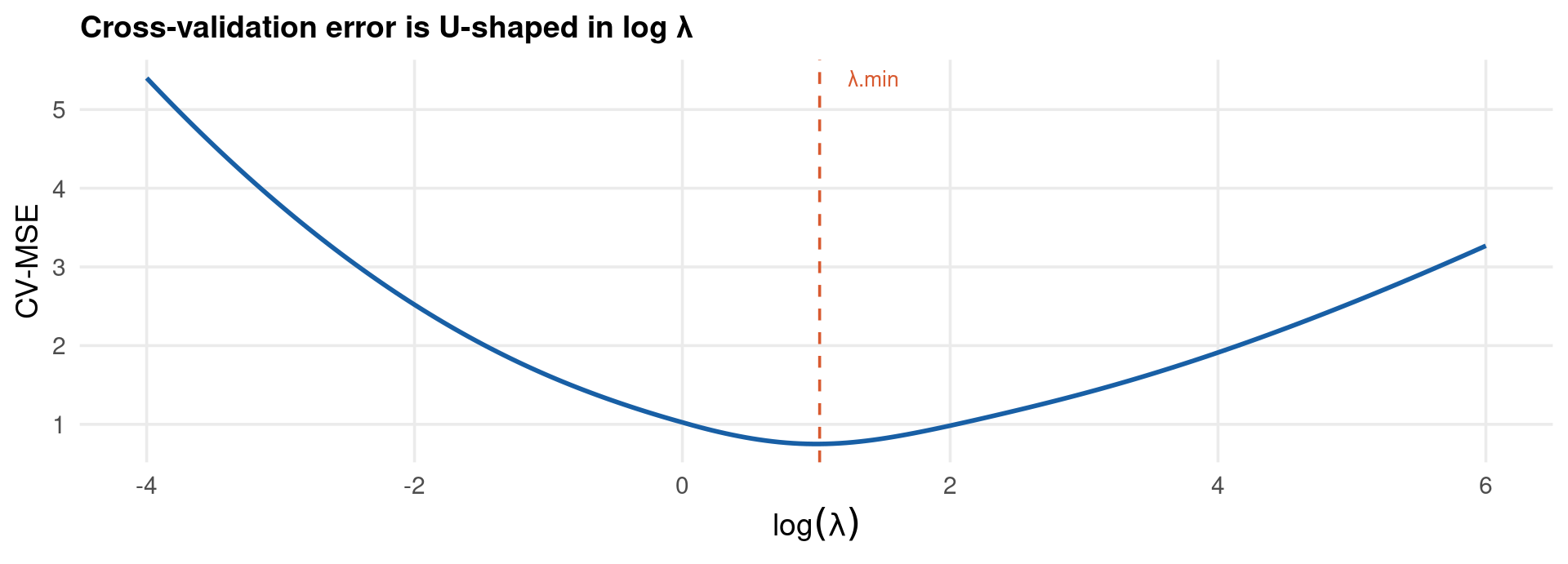
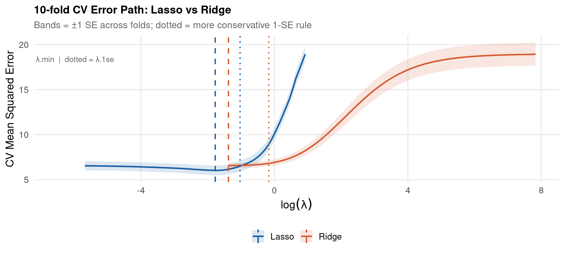
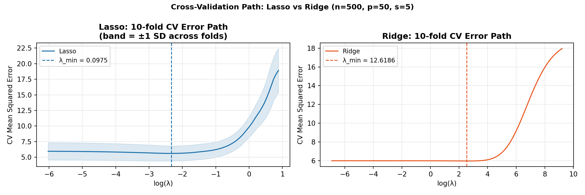
The cross-validation MSE is U-shaped in \(\log\lambda\):

• Left (\(\lambda \to 0\)): Ridge → OLS — low bias, high variance; CV-MSE high when predictors are collinear.
• Right (\(\lambda \to \infty\)): all coefficients → 0 — high bias, low variance; CV-MSE rises toward the variance of \(y\).
• Minimum: the bias–variance sweet spot. Two standard choices: \(\lambda_{\min}\) (lowest CV-MSE) and \(\lambda_{1\text{se}}\) (largest \(\lambda\) within one standard error — a more conservative, more heavily-shrunk model).

# Conceptual U-curve: illustrates the SHAPE of CV-MSE(λ); not a fit to data.
log_lam <- seq(-4, 6, length.out = 200)
# Flat-ish at small λ (OLS variance), rises at large λ (bias); gentle dip between.
cv_mse  <- 0.9 + 0.18 * (log_lam - 1)^2 / (1 + 0.15 * pmax(log_lam, 0)) -
           0.15 * exp(-(log_lam - 1)^2)
lam_min_x <- log_lam[which.min(cv_mse)]
ggplot(tibble(log_lam, cv_mse), aes(log_lam, cv_mse)) +
  geom_line(colour = col_main, linewidth = 1) +
  geom_vline(xintercept = lam_min_x, linetype = "dashed", colour = col_accent) +
  annotate("text", x = lam_min_x + 0.4, y = max(cv_mse),
           label = "λ.min", colour = col_accent, size = 3.5) +
  labs(x = expression(log(lambda)), y = "CV-MSE",
       title = "Cross-validation error is U-shaped in log λ") +
  theme_lecture + NULL

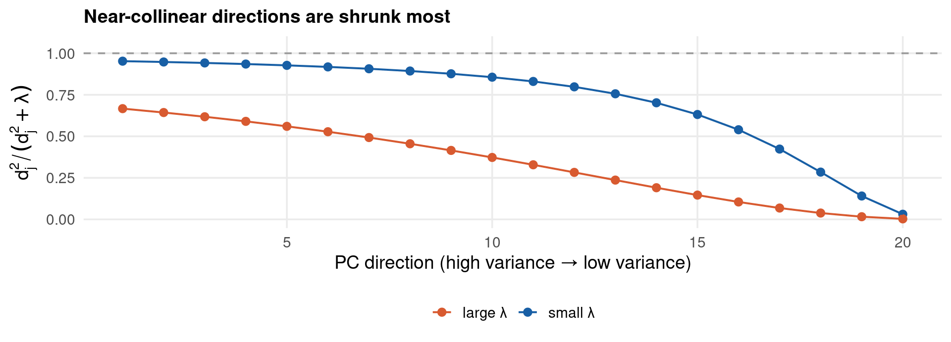
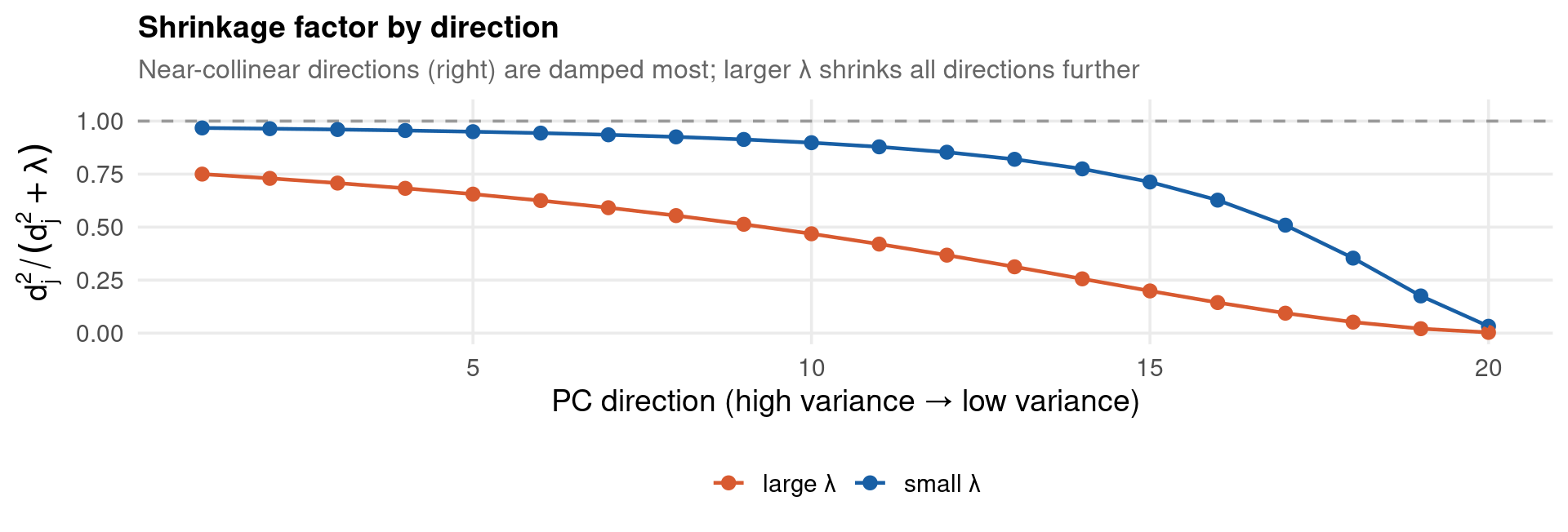
Writing the fit in the SVD basis, each principal-component direction \(j\) is shrunk by a factor

\[f_j(\lambda) = \frac{d_j^2}{d_j^2 + \lambda},\]

where \(d_j\) is the \(j\)-th singular value. High-variance directions (large \(d_j\)) are barely touched; near-collinear directions (small \(d_j\)) are shrunk hardest. This is exactly why Ridge stabilises collinear designs — it damps the directions OLS cannot estimate reliably.

# Conceptual: shrinkage factor across ordered PC directions for two λ values.
d_sq  <- (seq(1, 0.04, length.out = 20))^2   # decreasing singular values²
sf <- bind_rows(
  tibble(PC = 1:20, sf = d_sq / (d_sq + 0.05), rule = "small λ"),
  tibble(PC = 1:20, sf = d_sq / (d_sq + 0.50), rule = "large λ")
)
ggplot(sf, aes(PC, sf, colour = rule)) +
  geom_hline(yintercept = 1, colour = "grey60", linetype = "dashed") +
  geom_point(size = 2.4) + geom_line(linewidth = 0.7) +
  scale_colour_manual(values = c("small λ" = col_main, "large λ" = col_accent)) +
  scale_y_continuous(limits = c(0, 1.05)) +
  labs(x = "PC direction (high variance → low variance)",
       y = expression(d[j]^2 / (d[j]^2 + lambda)),
       title = "Near-collinear directions are shrunk most", colour = NULL) +
  theme_lecture + NULL

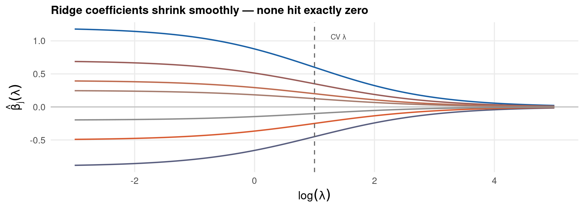
As \(\lambda\) increases, every coefficient shrinks continuously and smoothly toward zero — but, unlike Lasso, never reaches exactly zero. Ridge keeps all predictors; it only damps them. The vertical line marks the CV-selected \(\lambda\).

# Conceptual trace: smooth shrinkage of several coefficients toward 0.
log_lam <- seq(-3, 5, length.out = 120)
starts  <- c(1.2, -0.9, 0.7, -0.5, 0.4, 0.25, -0.2)
trace_df <- bind_rows(lapply(seq_along(starts), function(k)
  tibble(log_lam, beta = starts[k] / (1 + exp(log_lam - 1)), j = factor(k))))
ggplot(trace_df, aes(log_lam, beta, colour = j)) +
  geom_hline(yintercept = 0, colour = "grey75") +
  geom_line(linewidth = 0.8) +
  geom_vline(xintercept = 1, linetype = "dashed", colour = "grey40") +
  annotate("text", x = 1.4, y = max(trace_df$beta) * 0.9,
           label = "CV λ", colour = "grey30", size = 3.2) +
  scale_colour_manual(
    values = colorRampPalette(c(col_main, col_accent, col_muted))(length(starts)),
    guide = "none") +
  labs(x = expression(log(lambda)), y = expression(hat(beta)[j](lambda)),
       title = "Ridge coefficients shrink smoothly — none hit exactly zero") +
  theme_lecture + NULL

Ridge — The Bias–Variance Tradeoff, Conceptually

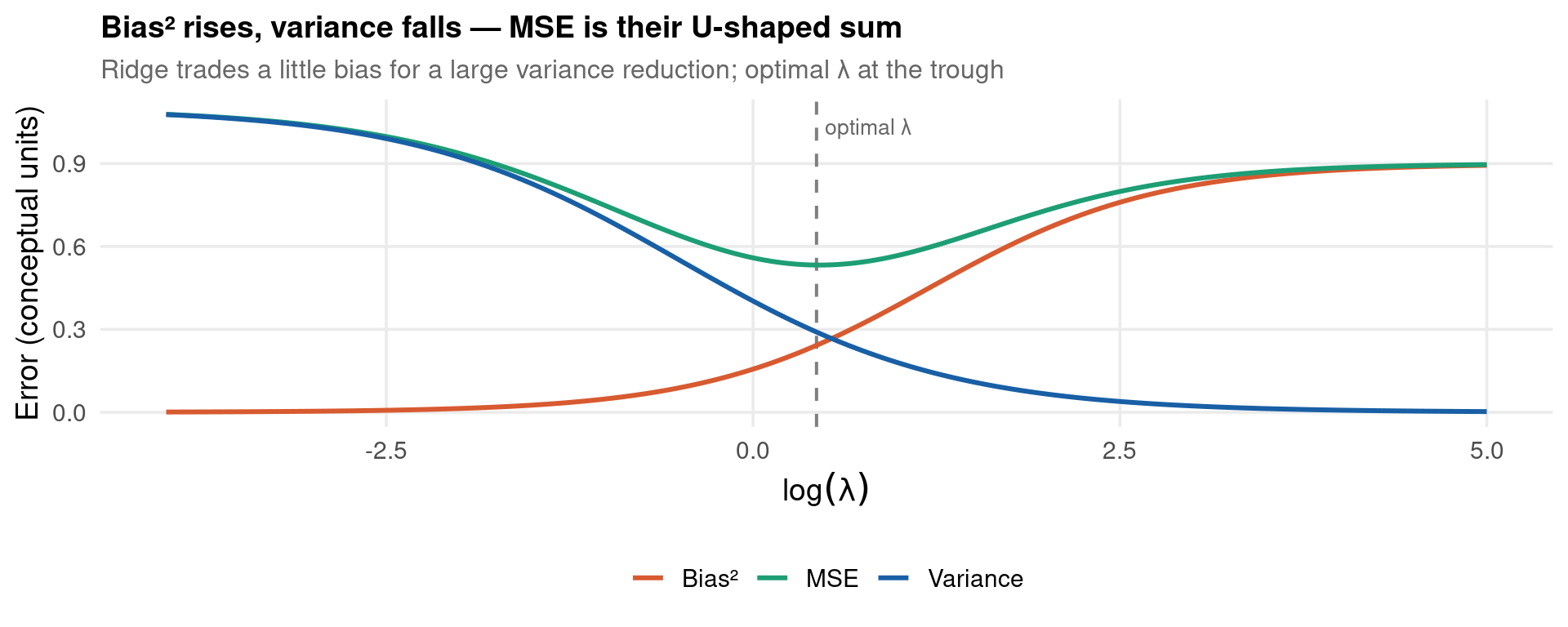
Ridge buys a reduction in variance at the cost of bias. The mean-squared error of the coefficient estimates decomposes exactly as

\[\text{MSE}(\lambda) = \underbrace{\text{Bias}(\lambda)^2}_{\uparrow \text{ in } \lambda} + \underbrace{\text{Variance}(\lambda)}_{\downarrow \text{ in } \lambda}.\]

As \(\lambda\) grows, coefficients are pulled toward zero: bias rises (we systematically under-shoot) while variance falls (estimates stop chasing noise). Their sum is U-shaped, and the CV-selected \(\lambda\) sits near its trough. This is why a biased estimator can beat OLS on total error — and it is a property of the estimator, not of any one dataset, so we show it here as a concept.

# Conceptual decomposition: illustrates the SHAPE of each component vs log λ.
# Not a Monte Carlo and not a fit to data — the analytic forms below are the
# textbook shapes (bias² rising, variance falling, MSE their U-shaped sum).
log_lam <- seq(-4, 5, length.out = 200)
variance <- 1.1 / (1 + exp(1.1 * (log_lam + 0.5)))   # high at small λ, →0
bias_sq  <- 0.9 / (1 + exp(-1.3 * (log_lam - 1.2)))   # ~0 at small λ, rising
mse      <- bias_sq + variance
lam_star <- log_lam[which.min(mse)]

bv <- bind_rows(
  tibble(log_lam, value = bias_sq, component = "Bias²"),
  tibble(log_lam, value = variance, component = "Variance"),
  tibble(log_lam, value = mse,      component = "MSE")
)
p_bv <- ggplot(bv, aes(log_lam, value, colour = component)) +
  geom_vline(xintercept = lam_star, linetype = "dashed",
             colour = "grey50", linewidth = 0.7) +
  geom_line(linewidth = 1.05) +
  scale_colour_manual(values = c("Bias²" = col_accent,
                                 "Variance" = col_main, "MSE" = col_ok)) +
  annotate("text", x = lam_star + 0.35, y = max(mse) * 0.96,
           label = "optimal λ", colour = "grey40", size = 3.5) +
  labs(x = expression(log(lambda)), y = "Error (conceptual units)",
       title = "Bias² rises, variance falls — MSE is their U-shaped sum",
       subtitle = "Ridge trades a little bias for a large variance reduction; optimal λ at the trough",
       colour = NULL) +
  theme_lecture
print(p_bv)

📝  Why this matters for econometrics

OLS is unbiased but, under collinearity, its variance explodes — so its MSE is dominated by the variance term. Ridge accepts a small bias to cut that variance, lowering total MSE. The existence of a \(\lambda\) where \(\text{MSE}_{\text{ridge}} < \text{MSE}_{\text{OLS}}\) is guaranteed (Hoerl & Kennard 1970); CV is how we locate it in practice.

Ridge — Results & Reporting

• What to report
• Reporting template
• Interpretation tips

Mandatory items when reporting Ridge regression results:

Item	What to state	Example
Estimator	Ridge regression, not OLS	“We use Ridge regression with \(\ell_2\) penalty”
Standardisation	Were predictors standardised?	“All predictors standardised to unit variance”
λ selection	Method, folds, criterion	“10-fold CV minimising MSE, \(\lambda^* = 0.312\)”
df(λ)	Effective parameters	“df(λ) = 11.4 (OLS df = 20)”
OOS performance	Test-set RMSE and R²	“Test RMSE = 1.61 vs OLS 2.84”
Visualisation	CV path and coefficient trace	Include cvplot / coefpath

Important

Never report: \(t\)-statistics, \(p\)-values, or confidence intervals on individual Ridge \(\hat\beta_j\). Ridge coefficients are biased — conventional SEs do not apply. For causal inference use DML with Ridge as the nuisance estimator.

A Ridge results table reports the regularisation choices and out-of-sample fit, never \(t\)/\(p\)-values on individual penalised coefficients. Use this skeleton (fill with your own CV output):

Quantity	What to report
Estimator	Ridge (\(\ell_2\)), predictors standardised
\(\lambda\) selection	10-fold CV minimising MSE; report \(\lambda_{\min}\) (and \(\lambda_{1\text{se}}\) if used)
Effective df	\(\text{df}(\lambda)=\sum_j d_j^2/(d_j^2+\lambda)\), alongside the OLS parameter count
OOS fit	Test-set RMSE and \(R^2\), vs an OLS / TWFE baseline
Condition number	\(\kappa(\mathbf{X}^\top\mathbf{X})\) to document the collinearity Ridge addresses
Visualisation	CV path (U-shape) and coefficient trace (smooth shrinkage)

LaTeX skeleton (booktabs) — replace the placeholders with your fitted values:

\begin{table}[t]\centering
\caption{Ridge regression: regularisation and out-of-sample fit}
\begin{tabular}{lcc}
\toprule
 & OLS & Ridge ($\hat\lambda$) \\
\midrule
Effective df      & $p$        & $\text{df}(\hat\lambda)$ \\
Test RMSE         & \dots      & \dots \\
Test $R^2$        & \dots      & \dots \\
\bottomrule
\end{tabular}
\end{table}

The wagepan worked example in Steps 1–3 produces exactly these quantities; xtable/tabulate (R/Python) or esttab (Stata) turn the fitted objects into this table.

Five principles for reading Ridge output:

1. Ridge \(\hat\beta_j\) ≠ OLS \(\hat\beta_j\) — they solve different problems. Ridge minimises a penalised criterion; its coefficients are biased toward zero by \(\frac{d_j^2}{d_j^2+\lambda}\) per PC direction. Do not compare magnitudes directly with OLS.
2. Signs are reliable; magnitudes are attenuated. Direction (sign, rank ordering) is informative; absolute values are not. Never state: “\(\hat\beta_j^{\text{ridge}} = 0.15\) implies a 0.15-unit causal effect.”
3. Large shrinkage signals a problematic direction. \(|\hat\beta_j^{\text{ridge}}| \ll |\hat\beta_j^{\text{OLS}}|\) means \(x_j\) lies in a near-collinear PC direction. The shrinkage is a diagnostic, not evidence of irrelevance.
4. df(λ) is the effective model size — report it. \(\text{df}(\lambda) = 8\) with \(p = 20\) means the model has effectively 8 free parameters. Use this instead of \(p\) when comparing regularised models.
5. For causal inference: Ridge is infrastructure. Ridge as a nuisance estimator in DML → report only the second-stage \(\hat\theta\) and its confidence interval.

# Conceptual: the per-direction shrinkage factor d²/(d²+λ) as the singular value
# d falls. High-variance directions (large d) are barely shrunk; near-collinear
# directions (small d) are shrunk toward zero. Illustrative — not a fit to data.
d_vals <- seq(3, 0.1, length.out = 20)        # singular values, large → small
tibble(
  PC      = 1:20,
  small_l = d_vals^2 / (d_vals^2 + 0.3),
  large_l = d_vals^2 / (d_vals^2 + 3.0)
) %>%
  pivot_longer(c(small_l, large_l), names_to = "rule", values_to = "sf") %>%
  mutate(rule = recode(rule, small_l = "small λ", large_l = "large λ")) %>%
  ggplot(aes(PC, sf, colour = rule)) +
    geom_hline(yintercept = 1, colour = "grey60", linetype = "dashed") +
    geom_point(size = 2.4) + geom_line(linewidth = 0.8) +
    scale_colour_manual(values = c("small λ" = col_main, "large λ" = col_accent)) +
    scale_y_continuous(limits = c(0, 1.05),
      name = expression(d[j]^2 / (d[j]^2 + lambda))) +
    labs(x = "PC direction (high variance → low variance)",
         title = "Shrinkage factor by direction",
         subtitle = "Near-collinear directions (right) are damped most; larger λ shrinks all directions further",
         colour = NULL) + theme_lecture + NULL

Ridge — The Econometric Heritage: James-Stein

Ridge did not arrive from computer science — it has deep roots in classical econometric shrinkage.

The James-Stein estimator (James & Stein 1961; Stein 1956) proved something that shocked statisticians: when estimating \(G \geq 3\) means simultaneously, the sample mean is inadmissible — a shrinkage estimator dominates it in total MSE.

\[\hat{\boldsymbol\theta}^{JS} = \left(1 - \frac{(G-2)\,\sigma^2}{\|\hat{\boldsymbol\theta}^{OLS}\|^2}\right)\hat{\boldsymbol\theta}^{OLS}\]

This is shrinkage toward zero with a data-driven factor — exactly Ridge’s mechanism, derived two decades before machine learning adopted it.

The connection to Ridge (Hansen 2022, §28.20–28.24):

Concept	James-Stein	Ridge
Mechanism	Shrink \(\hat{\boldsymbol\theta}^{OLS}\) toward 0	Shrink \(\hat{\boldsymbol\beta}^{OLS}\) toward 0
Justification	MSE dominance (admissibility)	MSE: bias² + variance trade-off
Shrinkage factor	\(1 - (G-2)\sigma^2/\|\hat\theta\|^2\)	\(d_j^2/(d_j^2 + \lambda)\) per PC
Guarantee	Provably dominates OLS	\(\exists\,\lambda^*: \text{MSE} < \text{MSE}_{OLS}\)

Ridge — Heritage: Group James-Stein

Group James-Stein (Hansen §28.24) — the precursor to Elastic Net’s grouping:

\[\hat{\boldsymbol\theta}_g^{JS} = \hat{\boldsymbol\theta}_g\left(1 - \frac{K_g - 2}{\hat{\boldsymbol\theta}_g' \mathbf{V}_g^{-1}\hat{\boldsymbol\theta}_g}\right)_{+}\]

Each block of coefficients is shrunk separately. With positive-part trimming \((\cdot)_+\), blocks with small effects are shrunk exactly to zero — simultaneous shrinkage and selection, the same idea Elastic Net formalises with the \(\ell_1 + \ell_2\) penalty.

📝  The shrinkage lineage

Stein (1956) → James-Stein (1961) → Group James-Stein → Ridge → Elastic Net. The econometric tradition of shrinkage long predates the ML literature; Ridge is its continuous, penalty-based formulation.

Reference: Hansen (2022) Ch. 28, §28.19–28.25.

Ridge — Application: wagepan Union Premium

Same dataset, different regularisation. We now use Ridge (\(\alpha=0\)) instead of Lasso. All controls are retained — Ridge shrinks them, never zeros them. The question: does the union premium estimate differ from TWFE and Post-Lasso OLS?

• R
• Python
• Stata

library(wooldridge)
library(plm)
library(sandwich)

# - Load wagepan from the wooldridge package (hard fail if not installed)
wp2 <- wagepan

# - Candidate controls for the union-premium specification
ctrl <- c("exper", "expersq", "married", "educ", "black", "hisp", "south")
wp2  <- wp2[, c("nr", "year", "lwage", "union", ctrl)]

# - Within-transform (remove individual fixed effect)
wp2_dm <- wp2 %>%
  group_by(nr) %>%
  mutate(across(where(is.numeric),
                ~ . - mean(., na.rm = TRUE) + mean(wp2[[cur_column()]], na.rm = TRUE))) %>%
  ungroup()

# - Control matrix: demeaned covariates + year dummies
yr_dummies <- model.matrix(~ factor(year) - 1, data = wp2_dm)[, -1]
num_cols   <- setdiff(names(wp2_dm), c("nr", "year", "lwage", "union"))
ctrl_r2    <- cbind(as.matrix(wp2_dm[, num_cols]), yr_dummies)
y_r2       <- wp2_dm$lwage
D_r2       <- wp2_dm$union

# - TWFE baseline via plm (two-way within, cluster-robust SE)
pdat2    <- pdata.frame(wp2, index = c("nr", "year"))
twfe_m2  <- plm(lwage ~ union + exper + expersq + married + educ,
                data = pdat2, model = "within", effect = "twoways")
b_twfe2  <- coef(twfe_m2)["union"]
se_twfe2 <- sqrt(vcovHC(twfe_m2, cluster = "group")["union", "union"])

cat(sprintf("TWFE union premium: %.4f  (clustered SE: %.4f)\n", b_twfe2, se_twfe2))

TWFE union premium: 0.0800  (clustered SE: 0.0227)

cat(sprintf("Control matrix: %d obs × %d predictors\n", nrow(ctrl_r2), ncol(ctrl_r2)))

Control matrix: 4360 obs × 14 predictors

# Ridge with 10-fold CV — D included in the penalty (shrink all controls)
# For the union coefficient we use the post-Ridge strategy:
# partial out controls via Ridge, then OLS of residuals on D
set.seed(SEED)
cv_r_wp  <- cv.glmnet(
  x           = ctrl_r2,
  y           = y_r2,
  alpha       = 0,
  nfolds      = N_CV_FOLDS,
  standardize = TRUE
)
cv_d_wp  <- cv.glmnet(
  x           = ctrl_r2,
  y           = D_r2,
  alpha       = 0,
  nfolds      = N_CV_FOLDS,
  standardize = TRUE
)

# Partialled residuals
yres_r2 <- y_r2 - predict(cv_r_wp, ctrl_r2, s="lambda.min")
Dres_r2 <- D_r2 - predict(cv_d_wp, ctrl_r2, s="lambda.min")

# OLS of y-residuals on D-residuals (FWL / Robinson 1988)
ridge_ols2 <- lm(yres_r2 ~ Dres_r2)
b_ridge2   <- coef(ridge_ols2)["Dres_r2"]
se_ridge2  <- sqrt(vcovHC(ridge_ols2,"HC3")["Dres_r2","Dres_r2"])

cat(sprintf("Ridge (partial-out) union premium: %.4f  (HC3 SE: %.4f)\n",
            b_ridge2, se_ridge2))

Ridge (partial-out) union premium: 0.0827  (HC3 SE: 0.0183)

# Effective df at lambda.min
d2_r2 <- svd(ctrl_r2, nu=0, nv=0)$d^2
df_r2 <- sum(d2_r2/(d2_r2 + cv_r_wp$lambda.min))
cat(sprintf("Ridge effective df: %.1f  (OLS df = %d)\n", df_r2, ncol(ctrl_r2)))

Ridge effective df: 11.0  (OLS df = 14)

# - Which controls Ridge shrinks most — the numbers behind the shrinkage
# Ridge never zeroes; we show OLS vs Ridge coefficients on the SAME controls so
# the shrinkage is visible. Largest |Ridge coef| = controls Ridge leans on most.
b_ridge_ctrl <- as.numeric(coef(cv_r_wp, s = "lambda.min"))[-1]   # drop intercept
ols_full     <- lm(y_r2 ~ ctrl_r2)
b_ols_ctrl   <- coef(ols_full)[-1]
shrink_tbl <- tibble(
  Control      = colnames(ctrl_r2),
  `OLS b`      = round(as.numeric(b_ols_ctrl), 4),
  `Ridge b`    = round(b_ridge_ctrl, 4),
  `Shrunk by %`= round(100 * (1 - b_ridge_ctrl / as.numeric(b_ols_ctrl)), 1)
)
shrink_tbl <- arrange(shrink_tbl, desc(abs(`Ridge b`)))
cat("\nTop controls by |Ridge coefficient| (OLS vs Ridge):\n")

Top controls by |Ridge coefficient| (OLS vs Ridge):

print(as.data.frame(head(shrink_tbl, 10)), row.names = FALSE)

          Control   OLS b Ridge b Shrunk by %
 factor(year)1987      NA  0.1520          NA
 factor(year)1986 -0.0321  0.1172       465.0
            south  0.0973  0.1030        -5.9
 factor(year)1985 -0.0464  0.0925       299.2
 factor(year)1984 -0.0394  0.0815       306.8
          married  0.0483  0.0634       -31.5
            exper  0.1323  0.0584        55.8
 factor(year)1983 -0.0443  0.0520       217.4
 factor(year)1982 -0.0123  0.0518       520.4
 factor(year)1981  0.0183  0.0429      -134.1

tibble(
  Estimator = c("TWFE", "Ridge (partial-out)"),
  `Union premium` = c(b_twfe2, b_ridge2),
  `SE`            = c(se_twfe2, se_ridge2),
  `λ*`            = c("—", sprintf("%.4f", cv_r_wp$lambda.min)),
  `eff. df`       = c("5 (OLS)", sprintf("%.1f", df_r2))
) %>%
  kbl(caption="wagepan: Union Premium — TWFE vs Ridge (partial-out)", digits=4) %>%
  kable_styling(font_size=20, full_width=TRUE) %>%
  row_spec(2, bold=TRUE, color="white", background=col_main)

wagepan: Union Premium — TWFE vs Ridge (partial-out)

Estimator	Union premium	SE	λ*	eff. df
TWFE	0.0800	0.0227	—	5 (OLS)
Ridge (partial-out)	0.0827	0.0183	0.0145	11.0

import pandas as pd, numpy as np, warnings
from sklearn.linear_model import RidgeCV
from sklearn.preprocessing import StandardScaler
warnings.filterwarnings('ignore')

# Self-contained: reload wagepan, demean, build controls
try:
    import wooldridge as woo
    wp_r = woo.data("wagepan")
except Exception:
    wp_r = pd.read_csv("../data/wagepan.csv")

ctrl_c = [c for c in ["exper","expersq","married","educ","black","hisp","south","smsa",
                       "agric","bus","construc","ndurman","trcommpu","trade",
                       "services","profserv","profocc","clerocc","servocc"]
          if c in wp_r.columns]
use_c = ["nr","year","lwage","union"] + ctrl_c
wp_r  = wp_r[[c for c in use_c if c in wp_r.columns]].dropna()
num_c = [c for c in wp_r.columns if c not in ["nr","year"]]
wp_r[num_c] = wp_r[num_c] - wp_r.groupby("nr")[num_c].transform("mean")
yr_d  = pd.get_dummies(wp_r["year"], prefix="yr", drop_first=True).astype(float)
ctrl_all_r = pd.concat([wp_r[ctrl_c], yr_d], axis=1).values
y_r_py = wp_r["lwage"].values
D_r_py = wp_r["union"].values

# TWFE baseline
X_twfe_r = np.column_stack([D_r_py, ctrl_all_r])
b_twfe_r  = np.linalg.lstsq(X_twfe_r, y_r_py, rcond=None)[0][0]
print(f"TWFE union premium: {b_twfe_r:.4f}")

TWFE union premium: 0.0796

# Ridge partial-out
sc2 = StandardScaler().fit(ctrl_all_r)
X_sc2 = sc2.transform(ctrl_all_r)
alphas_r = np.logspace(-2, 4, 100)
ridge_y_py = RidgeCV(alphas=alphas_r, cv=N_CV_FOLDS).fit(X_sc2, y_r_py)
ridge_d_py = RidgeCV(alphas=alphas_r, cv=N_CV_FOLDS).fit(X_sc2, D_r_py)

yres_py = y_r_py - ridge_y_py.predict(X_sc2)
Dres_py = D_r_py - ridge_d_py.predict(X_sc2)
b_ridge_py  = np.dot(Dres_py, yres_py) / np.dot(Dres_py, Dres_py)
resid_rr    = yres_py - b_ridge_py * Dres_py
psi_rr      = Dres_py * resid_rr
se_ridge_py = ((Dres_py**2).mean()**(-2) * (psi_rr**2).mean() / len(y_r_py))**0.5

d2_py2 = np.linalg.svd(X_sc2, compute_uv=False)**2
df_py2 = np.sum(d2_py2 / (d2_py2 + ridge_y_py.alpha_))
print(f"Ridge union premium: {b_ridge_py:.4f}  SE: {se_ridge_py:.4f}")

Ridge union premium: 0.0797  SE: 0.0183

print(f"Ridge λ*: {ridge_y_py.alpha_:.4f}  effective df: {df_py2:.1f}")

Ridge λ*: 6.1359  effective df: 12.9

from tabulate import tabulate
print(tabulate([
    ["TWFE",                f"{b_twfe_r:.4f}", "demeaned OLS", "—"],
    ["Ridge (partial-out)", f"{b_ridge_py:.4f}", f"df {df_py2:.1f}", f"{ridge_y_py.alpha_:.4f}"]],
    headers=["Estimator","Union premium","Controls/df","λ*"],
    tablefmt="rounded_outline"))

╭─────────────────────┬─────────────────┬───────────────┬────────╮
│ Estimator           │   Union premium │ Controls/df   │ λ*     │
├─────────────────────┼─────────────────┼───────────────┼────────┤
│ TWFE                │          0.0796 │ demeaned OLS  │ —      │
│ Ridge (partial-out) │          0.0797 │ df 12.9       │ 6.1359 │
╰─────────────────────┴─────────────────┴───────────────┴────────╯

* Ridge = elasticnet with alpha(0)
* We use the partial-out approach:
*   (1) Ridge y on X → residuals y_tilde
*   (2) Ridge D on X → residuals D_tilde
*   (3) OLS y_tilde on D_tilde → beta_union (Robinson 1988)

frause wagepan, clear
xtset nr year

* - Robust within-demean: only demean variables that actually exist
local ctrl_dm ""
foreach v in exper expersq married educ black hisp south {
    quietly bysort nr: egen `v'_m = mean(`v')
    quietly gen `v'_dm = `v' - `v'_m
    local ctrl_dm "`ctrl_dm' `v'_dm"
}
foreach v in lwage union {
    quietly bysort nr: egen `v'_m = mean(`v')
    quietly gen `v'_dm = `v' - `v'_m
}

* TWFE baseline
xtreg lwage union exper expersq married educ i.year, fe vce(cluster nr)
estimates store TWFE_R
display "TWFE union premium: " %8.4f _b[union]

* Ridge of outcome on controls (alpha=0 = pure ℓ₂, 10-fold CV)
elasticnet linear lwage_dm `ctrl_dm', alpha(0) selection(cv, folds(10)) nolog
predict yhat
gen yres = lwage_dm - yhat
lassoinfo

* Ridge of treatment on controls
elasticnet linear union_dm `ctrl_dm', alpha(0) selection(cv, folds(10)) nolog
predict Dhat
gen Dres = union_dm - Dhat

* Step 3: OLS of y-residuals on D-residuals (Robinson/FWL)
regress yres Dres, robust
local b_ridge  = _b[Dres]
local se_ridge = _se[Dres]
display "Ridge partial-out union premium: " %8.4f `b_ridge'

* Comparison (display avoids esttab's fragile cross-model coefficient renaming)
quietly xtreg lwage union exper expersq married educ i.year, fe vce(cluster nr)
display _newline "wagepan: Union Premium — TWFE vs Ridge (partial-out)"
display "  TWFE            : " %8.4f _b[union]  "  (cluster SE " %8.4f _se[union]  ")"
display "  Ridge partial   : " %8.4f `b_ridge' "  (robust SE  " %8.4f `se_ridge' ")"

Panel variable: nr (strongly balanced)
 Time variable: year, 1980 to 1987
         Delta: 1 unit




note: educ omitted because of collinearity.
note: 1987.year omitted because of collinearity.

Fixed-effects (within) regression               Number of obs     =      4,360
Group variable: nr                              Number of groups  =        545

R-squared:                                      Obs per group:
     Within  = 0.1806                                         min =          8
     Between = 0.0005                                         avg =        8.0
     Overall = 0.0635                                         max =          8

                                                F(10, 544)        =      46.59
corr(u_i, Xb) = -0.1212                         Prob > F          =     0.0000

                                   (Std. err. adjusted for 545 clusters in nr)
------------------------------------------------------------------------------
             |               Robust
       lwage | Coefficient  std. err.      t    P>|t|     [95% conf. interval]
-------------+----------------------------------------------------------------
       union |   .0800019   .0227431     3.52   0.000     .0353268    .1246769
       exper |   .1321464    .012008    11.00   0.000     .1085586    .1557342
     expersq |  -.0051855   .0008102    -6.40   0.000    -.0067771   -.0035939
     married |   .0466804   .0210038     2.22   0.027     .0054218    .0879389
        educ |          0  (omitted)
             |
        year |
       1981  |   .0190448   .0227267     0.84   0.402     -.025598    .0636876
       1982  |   -.011322   .0212167    -0.53   0.594    -.0529987    .0303547
       1983  |  -.0419955   .0205087    -2.05   0.041    -.0822814   -.0017096
       1984  |  -.0384709   .0211722    -1.82   0.070    -.0800601    .0031183
       1985  |  -.0432498    .017595    -2.46   0.014    -.0778122   -.0086874
       1986  |  -.0273819   .0162181    -1.69   0.092    -.0592396    .0044757
       1987  |          0  (omitted)
             |
       _cons |    1.02764   .0398919    25.76   0.000     .9492785    1.106001
-------------+----------------------------------------------------------------
     sigma_u |   .4009279
     sigma_e |  .35099001
         rho |  .56612236   (fraction of variance due to u_i)
------------------------------------------------------------------------------


TWFE union premium:   0.0800


Elastic net linear model                         No. of obs        =      4,360
                                                 No. of covariates =          4
Selection: Cross-validation                      No. of CV folds   =         10

-------------------------------------------------------------------------------
               |                               No. of      Out-of-      CV mean
               |                              nonzero       sample   prediction
alpha       ID |     Description      lambda    coef.    R-squared        error
---------------+---------------------------------------------------------------
0.000          |
             1 |    first lambda    145.1022        4      -0.0002     .1312307
            99 |   lambda before     .015925        4       0.1709     .1087772
         * 100 | selected lambda    .0145102        4       0.1712     .1087447
-------------------------------------------------------------------------------
* alpha and lambda selected by cross-validation.

(options xb penalized assumed; linear prediction with penalized coefficients)

    Estimate: active
     Command: elasticnet
---------------------------------------------------------------------------
            |                                                        No. of
  Dependent |           Selection  Selection                       selected
   variable |    Model     method  criterion     alpha    lambda  variables
------------+--------------------------------------------------------------
   lwage_dm |   linear         cv    CV min.     0.000  .0145102          4
---------------------------------------------------------------------------


Elastic net linear model                         No. of obs        =      4,360
                                                 No. of covariates =          4
Selection: Cross-validation                      No. of CV folds   =         10

-------------------------------------------------------------------------------
               |                               No. of      Out-of-      CV mean
               |                              nonzero       sample   prediction
alpha       ID |     Description      lambda    coef.    R-squared        error
---------------+---------------------------------------------------------------
0.000          |
             1 |    first lambda    6.702594        4      -0.0002     .0761595
            19 |   lambda before    1.255944        4       0.0001     .0761365
          * 20 | selected lambda    1.144369        4       0.0001     .0761365
            21 |    lambda after    1.042706        4       0.0001     .0761366
            92 |     last lambda    .0014108        4      -0.0011     .0762305
-------------------------------------------------------------------------------
* alpha and lambda selected by cross-validation.

(options xb penalized assumed; linear prediction with penalized coefficients)



Linear regression                               Number of obs     =      4,360
                                                F(1, 4358)        =      20.85
                                                Prob > F          =     0.0000
                                                R-squared         =     0.0049
                                                Root MSE          =     .32862

------------------------------------------------------------------------------
             |               Robust
        yres | Coefficient  std. err.      t    P>|t|     [95% conf. interval]
-------------+----------------------------------------------------------------
        Dres |   .0833633   .0182556     4.57   0.000     .0475729    .1191536
       _cons |  -4.64e-10   .0049768    -0.00   1.000     -.009757     .009757
------------------------------------------------------------------------------



Ridge partial-out union premium:   0.0834



wagepan: Union Premium — TWFE vs Ridge (partial-out)

  TWFE            :   0.0800  (cluster SE   0.0227)

  Ridge partial   :   0.0834  (robust SE    0.0183)

Ridge — Part Summary: Take-Home Notes

What Ridge does:

• Solves \(\hat\beta^R = (\mathbf{X}^\top\mathbf{X}+\lambda\mathbf{I})^{-1}\mathbf{X}^\top\mathbf{y}\)
• Shrinks all coefficients proportionally — never zeros
• SVD interpretation: shrinks by \(d_j^2/(d_j^2+\lambda)\) per PC direction
• Effective df = \(\sum_j d_j^2/(d_j^2+\lambda) < p\)
• Always defined, even when \(p > n\)

What you report:

• \(\hat\beta^{union}\) from the partial-out (FWL) approach
• \(\hat\lambda^*\) from CV and effective df
• CV path plot (U-shape) and coefficient trace (smooth)
• Never report \(t\)-statistics on individual Ridge \(\hat\beta_j\)

Connection to economics:

• Ridge = Bayesian shrinkage with Gaussian prior
• Dense DGP (macro indicators, factor models) → Ridge dominates Lasso
• PCR (Principal Component Regression) ≈ continuous Ridge
• Partial-out Ridge is a valid causal estimator (Robinson 1988 + Ridge nuisance)

Common mistakes:

• Using Ridge for variable selection (it cannot zero out)
• Reporting Ridge \(\hat\beta_j\) as unbiased causal effects
• Not standardising predictors before fitting

Ridge — Progress · What Still Lacks

• Progress over Lasso
• What still lacks

• ✓ No arbitrary variable elimination — Ridge respects dense signal; Lasso discards correlated controls arbitrarily
• ✓ Always unique, always defined — closed-form solution via SVD, no convergence issues
• ✓ Stable under collinearity — correlated predictors are treated symmetrically, not arbitrarily selected
• ✓ PCR connection — Ridge is a continuous version of principal component regression; effective df is interpretable

• ✗ No variable selection — all \(p\) predictors are retained; the model is never sparse
• ✗ Biased coefficients — \(\hat\beta_j^R\) is always biased toward zero; no unbiasedness guarantee on any individual coefficient
• ✗ Cannot identify key controls — no way to say “these 5 variables matter, the rest are noise”
• ✗ Inference requires correction — same as Lasso: conventional SEs invalid; use partial-out + HC3
• ✗ Dense DGP assumption — if truth is truly sparse, Lasso dominates in prediction accuracy

Ridge — Bibliography

Foundational:

• Hoerl & Kennard (1970). Ridge regression. doi:10.1080/00401706.1970.10488634
• Robinson (1988). Root-N-consistent semiparametric regression. doi:10.2307/1912705

Shrinkage heritage (James-Stein):

• Stein (1956). Inadmissibility of the usual estimator for the mean of a multivariate normal. Proc. 3rd Berkeley Symp. project euclid
• James & Stein (1961). Estimation with quadratic loss. Proc. 4th Berkeley Symp. project euclid
• Hansen (2016). Efficient shrinkage in parametric models. doi:10.1016/j.jeconom.2016.03.002

Economic forecasting:

• De Mol, Giannone & Reichlin (2008). Forecasting using large number of predictors. doi:10.1016/j.jeconom.2008.08.011
• Stock & Watson (2012). Disentangling the 2007–2009 recession. doi:10.3386/w18094

Textbook:

• Hansen (2022). Econometrics. Princeton University Press — Ch. 28 (Stein shrinkage, §28.19–28.25), Ch. 29 §29.5–29.7 (Ridge)
• ISLR §6.2.1 (James et al. 2023)
• Hastie, Tibshirani & Wainwright (2015) Statistical Learning with Sparsity Ch. 2

Ridge — Exercises

1. Effective degrees of freedom — on wagepan, fit Ridge with 10-fold CV. Report \(\hat\lambda^*\), effective df, and the union premium. Now double and halve \(\hat\lambda^*\). How do effective df and the premium change? Sketch the bias-variance curve.

2. Ridge vs Lasso on wagepan — compare the union premium from Post-Lasso OLS and Ridge (partial-out). Are they statistically different? Which has lower out-of-sample MSE for lwage? Why might the estimates differ?

3. PCR comparison — fit Principal Component Regression on wagepan with 5, 10, 15 components. Compare to Ridge. At what number of components does PCR ≈ Ridge?

4. Dense vs sparse simulation — generate (a) \(n=200\), \(p=40\), all \(\beta_j = 0.3\) (dense); (b) \(n=200\), \(p=40\), only \(\beta_1=2\) (sparse). Over 200 MC replications, which method — Ridge or Lasso — achieves lower test MSE in each DGP?

5. Bayesian interpretation — Ridge corresponds to a \(\mathcal{N}(0, \sigma^2/\lambda)\) prior. For the wagepan CV-selected \(\hat\lambda^*\), what is the implied prior variance on \(\beta_{union}\)? Is it reasonable? How would you change \(\lambda\) if you believed the union effect is large?

Ridge — Full Code

Complete, standalone scripts for this part — libraries loaded and configuration hard-coded, so each file runs on its own. Download the language you want:

R

⬇ Download ridge.R

Python

⬇ Download ridge.py

Stata

⬇ Download ridge.do

All code shown live on the step slides; these files bundle it for re-use.

Part IV — Elastic Net

“What if the truth is somewhere between sparse and dense?”

Lasso says: most controls are zero.
Ridge says: all controls matter a little.
In wagepan, occupation and industry come in groups — if one matters, they probably all do.
Elastic Net lets groups enter or leave together.

Elastic Net — Econometric Framework

Why neither Lasso nor Ridge is quite right for wagepan:

Controls in a wage equation come in correlated groups: - Occupation: professional, clerical, service, managerial - Industry: manufacturing, trade, services, transport - Region × year interactions

Lasso picks one from each correlated group and discards the rest — even when all are relevant confounders. Ridge keeps all of them with equal (undifferentiated) shrinkage. Elastic Net selects groups: if occupation matters, all occupation dummies enter together; if industry does not, all industry dummies leave together.

The Elastic Net wage model:

\[\hat{\boldsymbol\gamma}^{EN} = \arg\min_{\boldsymbol\gamma} \|\mathbf{y} - D\beta - \mathbf{X}\boldsymbol\gamma\|_2^2 + \lambda\left[\alpha\|\boldsymbol\gamma\|_1 + \frac{1-\alpha}{2}\|\boldsymbol\gamma\|_2^2\right]\]

\(\alpha \in (0,1)\) controls the mix: \(\alpha = 1\) recovers Lasso, \(\alpha = 0\) recovers Ridge. CV over a grid of \(\alpha\) values lets the data determine whether the control structure is sparse, dense, or grouped.

The grouping property (Zou & Hastie 2005): \[|\hat\gamma_j^{EN} - \hat\gamma_k^{EN}| \leq \frac{1}{\lambda(1-\alpha)}\sqrt{2(1-r_{jk})}\] where \(r_{jk}\) is the correlation between controls \(j\) and \(k\). As \(r_{jk} \to 1\), the two coefficients converge — occupation dummies with similar wage patterns are treated as a group.

Regularised Regression — Elastic Net: Motivation

• ① The problem with Lasso and Ridge alone
• ② The grouping effect
• ③ Callouts

Lasso fails when predictors are correlated. Ridge fails when the signal is sparse.

Both failures appear constantly in economic data:

The wage regression problem: Consider predicting wages from occupation cells, education levels, and their interactions. Education and experience are correlated. Occupation dummies within the same field are correlated. Lasso arbitrarily retains one education variable and drops its correlated partner — even if both independently contribute. Ridge retains all occupation dummies with equal shrinkage — including truly irrelevant ones.

The macro forecasting problem: GDP growth, industrial production, and retail sales move together (correlated group). Monetary policy indicators form another correlated group. Lasso picks one indicator per group; Ridge keeps hundreds. Elastic Net selects entire groups or drops them together.

The input-output problem: In price transmission models (e.g. retail prices across outlets), prices for the same product in nearby stores are highly correlated. Lasso selects one outlet and discards the others — losing the group signal. Ridge keeps all outlets but cannot zero out irrelevant product categories. Elastic Net handles both.

What Elastic Net does: combines both penalties: \[P_{\alpha}(\boldsymbol\beta) = \alpha\|\boldsymbol\beta\|_1 + \frac{1-\alpha}{2}\|\boldsymbol\beta\|_2^2\]

\(\alpha \in [0,1]\) is the mixing parameter: \(\alpha=1\) is Lasso, \(\alpha=0\) is Ridge. At any interior \(\alpha\), Elastic Net simultaneously selects variables (\(\ell_1\)) and handles groups (\(\ell_2\)).

Why correlated variables are problematic for Lasso:

Let \(x_j \approx x_k\) (highly correlated). Then \(\hat\beta_j^{\text{lasso}} + \hat\beta_k^{\text{lasso}}\) is well-determined but the individual values \(\hat\beta_j, \hat\beta_k\) are unstable — small data changes flip which variable Lasso picks.

The \(\ell_2\) component in Elastic Net resolves this. Zou & Hastie (2005) proved the grouping effect:

\[|\hat\beta_j^{\text{EN}} - \hat\beta_k^{\text{EN}}| \leq \frac{2\sqrt{2}\,\sigma}{\lambda(1-\alpha)}\sqrt{1 - \text{Cor}(x_j, x_k)}\]

When \(\text{Cor}(x_j, x_k) \to 1\): the bound \(\to 0\), so \(\hat\beta_j^{\text{EN}} \approx \hat\beta_k^{\text{EN}}\). When \(\alpha \to 1\) (Lasso): the bound \(\to \infty\), so no grouping guarantee.

In practice: Elastic Net either retains the whole correlated group (with similar shrunk coefficients) or drops all of them together. This is economically natural — an industry’s input prices tend to matter collectively or not at all.

Naive Elastic Net vs corrected EN:

The plain Elastic Net introduces additional shrinkage beyond what the \(\ell_1\) term requires. Zou & Hastie recommend the corrected Elastic Net:

\[\hat{\boldsymbol\beta}^{\text{EN,corrected}} = (1 + (1-\alpha)\lambda/2)\cdot\hat{\boldsymbol\beta}^{\text{EN}}\]

This rescales coefficients to remove the double-shrinkage bias. glmnet applies this correction by default.

⚠️  Two Hyperparameters Instead of One

Elastic Net has both \(\lambda\) (overall penalty strength) and \(\alpha\) (mixing ratio):

\[P(\beta) = \lambda\left[\alpha\|\beta\|_1 + \frac{1-\alpha}{2}\|\beta\|_2^2\right]\]

Standard practice: 2D grid search via CV over \(\alpha \in \{0.1, 0.25, 0.5, 0.75, 0.9\}\) and 100 \(\lambda\) values per \(\alpha\).

• Stata: elasticnet linear y varlist, alpha(0.1 0.25 0.5 0.75 0.9)
• R: Loop over alpha in cv.glmnet()
• Python: ElasticNetCV(l1_ratio=[0.1,0.25,0.5,0.75,0.9])

📝  Economic Rationale for \(\alpha\) Choice

\(\alpha\) value	Economic setting	Why
\(\alpha = 1\) (Lasso)	Independent predictors, sparse DGP	Few dominant variables; others are noise
\(\alpha = 0.5\)	Grouped predictors, mixed sparsity	Education × occupation cells; factor models
\(\alpha = 0.1\)	Highly collinear, dense signal	Macro indicators; input-output tables
\(\alpha = 0\) (Ridge)	All predictors matter equally	Dense signal; no selection needed

💡  Elastic Net: The Safe Default

Elastic Net dominates both Lasso and Ridge as a general-purpose estimator:

• When the DGP is sparse: EN with \(\alpha \to 1\) recovers Lasso
• When the DGP is dense/collinear: EN with \(\alpha \to 0\) recovers Ridge
• CV picks the right \(\alpha\) from the data

If unsure whether the DGP is sparse or dense, Elastic Net is the safe default.

Regularised Regression — Elastic Net: Mathematics I

The Elastic Net objective:

\[\hat{\boldsymbol\beta}^{\text{EN}} = \arg\min_{\boldsymbol\beta} \underbrace{\|\mathbf{y}-\mathbf{X}\boldsymbol\beta\|_2^2}_{\text{fit}} + \lambda\left[\underbrace{\alpha\|\boldsymbol\beta\|_1}_{\ell_1:\;\text{sparsity}} + \underbrace{\frac{1-\alpha}{2}\|\boldsymbol\beta\|_2^2}_{\ell_2:\;\text{stability}}\right]\]

Two penalty parameters: \(\lambda \geq 0\) (overall strength) and \(\alpha \in [0,1]\) (L1/L2 mix).

Constraint form — the Elastic Net constraint region is a rounded diamond:

\[\hat{\boldsymbol\beta}^{\text{EN}} = \arg\min_{\boldsymbol\beta}\|\mathbf{y}-\mathbf{X}\boldsymbol\beta\|_2^2 \quad\text{s.t.}\quad \alpha\|\boldsymbol\beta\|_1 + \frac{1-\alpha}{2}\|\boldsymbol\beta\|_2^2 \leq t\]

The constraint region is a convex combination of:

• the \(\ell_1\) diamond (Lasso) — has corners on axes → sparsity
• the \(\ell_2\) sphere (Ridge) — smooth surface → stability

The rounded diamond retains corners (so some coefficients are set to exactly zero) but the flat faces become curved (so correlated coefficients are not forced to be exactly equal to zero simultaneously). This is the geometric origin of the grouping effect.

Coordinate-wise soft-thresholding update — used by the coordinate descent algorithm:

\[\hat\beta_j^{\text{EN}} = \frac{S_{\alpha\lambda/2}\!\left(\frac{1}{n}\mathbf{x}_j^\top\tilde{\mathbf{y}}_j\right)}{1 + \lambda(1-\alpha)}\]

where \(\tilde{\mathbf{y}}_j = \mathbf{y} - \mathbf{X}_{-j}\hat{\boldsymbol\beta}_{-j}\) is the partial residual, and \(S_t(\cdot)\) is the soft-thresholding operator. The denominator \(1 + \lambda(1-\alpha)\) is the Ridge shrinkage factor — applied after the Lasso soft-threshold.

Comparison of update rules:

Method	Coordinate update
OLS	\(\hat\beta_j = \mathbf{x}_j^\top\tilde{\mathbf{y}}_j / \|\mathbf{x}_j\|^2\)
Ridge	\(\hat\beta_j^{\text{ridge}} = \mathbf{x}_j^\top\tilde{\mathbf{y}}_j / (\|\mathbf{x}_j\|^2 + \lambda)\)
Lasso	\(\hat\beta_j^{\text{lasso}} = S_{\lambda/2}(\mathbf{x}_j^\top\tilde{\mathbf{y}}_j) / \|\mathbf{x}_j\|^2\)
Elastic Net	\(\hat\beta_j^{\text{EN}} = S_{\alpha\lambda/2}(\mathbf{x}_j^\top\tilde{\mathbf{y}}_j) / (\|\mathbf{x}_j\|^2 + \lambda(1-\alpha))\)

Elastic Net first soft-thresholds with \(\alpha\lambda/2\) (Lasso component), then divides by \(1+\lambda(1-\alpha)\) (Ridge component). It is computationally as fast as Lasso.

Regularised Regression — Elastic Net: Mathematics II

Number of selected variables — a key advantage over Lasso:

Lasso can select at most \(\min(n, p)\) variables (its path selects one at a time). Elastic Net can select more than \(n\) variables simultaneously when \(\alpha < 1\) — critical when \(p \gg n\).

The \(\alpha\)-\(\lambda\) solution surface:

Each pair \((\alpha, \lambda)\) gives a different sparse model. The two-parameter solution surface is explored by holding \(\alpha\) fixed and tracing the \(\lambda\) path, then repeating for each \(\alpha\):

\[\mathcal{B} = \{\hat{\boldsymbol\beta}^{\text{EN}}(\alpha, \lambda) : \alpha \in [0,1],\, \lambda \geq 0\}\]

At any fixed \(\alpha\), the path is piecewise linear in \(\lambda\) (same as Lasso). Cross-validation selects \((\alpha^*, \lambda^*)\) jointly by minimising CV-MSE over the full grid.

Effective degrees of freedom (Zou, Hastie & Tibshirani 2007):

Let \(\hat{\mathcal{S}} = \{j : \hat\beta_j^{\text{EN}} \neq 0\}\) be the selected set. Then:

\[\text{df}^{\text{EN}}(\alpha, \lambda) \approx \text{tr}\!\left[\mathbf{X}_{\hat{\mathcal{S}}}(\mathbf{X}_{\hat{\mathcal{S}}}^\top\mathbf{X}_{\hat{\mathcal{S}}} + \lambda(1-\alpha)\mathbf{I})^{-1}\mathbf{X}_{\hat{\mathcal{S}}}^\top\right]\]

Interpretation: like Ridge df but only over the selected subspace. As \(\alpha \to 1\), this approaches the Lasso df \(= |\hat{\mathcal{S}}|\). As \(\alpha \to 0\), it approaches the Ridge df formula.

Post-Elastic Net OLS:

As with Lasso, the penalised Elastic Net coefficients are biased. After variable selection by EN, run OLS on the selected set:

\[\tilde{\boldsymbol\beta}^{\text{post-EN}} = (\mathbf{X}_{\hat{\mathcal{S}}}^\top\mathbf{X}_{\hat{\mathcal{S}}})^{-1}\mathbf{X}_{\hat{\mathcal{S}}}^\top\mathbf{y}\]

This is more stable than post-Lasso OLS when the selected set contains correlated predictors (because EN selected them as a group, not arbitrarily).

📝  Adaptive Elastic Net (Zou & Zhang 2009)

Replaces the \(\ell_1\) component with a weighted penalty:

\[P_{\alpha}^{\text{adapt}}(\boldsymbol\beta) = \alpha\sum_j \hat\omega_j|\beta_j| + \frac{1-\alpha}{2}\|\boldsymbol\beta\|_2^2\]

where \(\hat\omega_j = 1/|\hat\beta_j^{\text{OLS}}|^\gamma\). Large initial coefficients get small weights (kept); small initial coefficients get large weights (zeroed out).

Oracle property: achieves asymptotically correct variable selection AND handles grouped predictors simultaneously.

Implementations:

• R: hdm::rlasso() with adaptive weights; glmnet with penalty.factor
• Stata: lasso linear y x, selection(adaptive)

Reference: Zou & Zhang (2009). doi:10.1214/08-AOS625

Elastic Net — When It Excels and When It Fails

• ✓ Use Elastic Net when
• ✗ Do NOT use Elastic Net when

1. Correlated groups with sparse between-group signal — The canonical Elastic Net setting: predictors cluster into correlated groups (education levels, occupation categories, industry sectors, regional price series) and only some groups are relevant. Lasso breaks up groups arbitrarily; EN selects them intact.

2. \(p > n\) settings with grouped structure — Lasso selects at most \(n\) variables. Elastic Net can select more, crucial in microeconomic panels with many fixed effects or in text-as-data regressions with clustered word groups.

3. Uncertain DGP — sparse or dense? — When you cannot commit to Lasso or Ridge a priori, Elastic Net nests both. CV over \(\alpha \in \{0, 0.1, 0.5, 0.9, 1\}\) finds the right mix from the data.

4. DML nuisance estimation with grouped controls — In Double ML applications with industry × occupation × region cells as controls, EN selects entire meaningful cells rather than individual dummies scattered across correlated groups.

5. Macroeconomic forecasting with factor structure — When predictors cluster into correlated macro factors (real activity, financial conditions, inflation expectations), EN respects the factor structure: it selects entire factors or drops them, improving forecast interpretability.

💡  Choosing \(\alpha\) in Practice

Fit EN with alpha = (0.1, 0.25, 0.5, 0.75, 0.9) and let CV choose.

CV selects	Interpretation	Recommendation
\(\alpha = 1\) consistently	DGP is sparse	Switch to Lasso
\(\alpha = 0\) consistently	DGP is dense	Switch to Ridge
Interior \(\alpha\) (0.1–0.9)	Mixed structure	EN is genuinely needed

1. The DGP is clearly sparse with independent predictors — If predictors are nearly uncorrelated and the true model has a few large effects, Lasso achieves better selection accuracy with one fewer hyperparameter to tune.

2. Computational constraints with very large \(p\) — The 2D grid search over \((\alpha, \lambda)\) multiplies computation by the number of \(\alpha\) values. For \(p > 10^4\), fit Lasso and Ridge separately and compare, rather than a full EN grid.

3. You need oracle-valid post-selection inference — The oracle property is harder to establish for EN than for adaptive Lasso. For formal post-selection inference, post-double-selection Lasso (PDS) has cleaner theoretical guarantees.

4. The penalty structure is theoretically motivated — In structural estimation (DSGE, production functions), when the penalty has a Bayesian interpretation that maps to a specific prior, use the appropriate Lasso or Ridge depending on the prior. Elastic Net has a mixed prior without a clean structural interpretation.

⚠️  Elastic Net: Not a Theoretical Panacea

Elastic Net's main advantage is practical robustness to uncertainty about DGP structure — not theoretical superiority.

• If the DGP is known sparse: Lasso has sharper theory (oracle property, irrepresentability), fewer hyperparameters
• If the DGP is known dense: Ridge has a closed-form solution, SVD interpretation, and no sparsity-inducing bias
• EN is the right default when DGP structure is unknown and you want CV to decide

Elastic Net — Key Functions

Elastic Net has two hyperparameters: \(\alpha\) (mix) and \(\lambda\) (strength). The API differs slightly from Lasso/Ridge.

• R — glmnet
• Python — ElasticNetCV
• Stata — elasticnet
• Python
• Stata

# Elastic Net: 0 < alpha < 1
# Strategy: loop over α values, let CV choose λ for each, pick best (α*, λ*)
alphas <- c(0.1, 0.25, 0.5, 0.75, 0.9)

cv_list <- future_map(alphas, \(a)
  cv.glmnet(X, y, alpha = a, nfolds = N_CV_FOLDS),
  .options = furrr_options(seed = SEED))

# Best (α*, λ*) = combination with lowest cv$cvm at cv$lambda.min
best_idx  <- which.min(sapply(cv_list, function(cv) min(cv$cvm)))
cv_best   <- cv_list[[best_idx]]
alpha_best <- alphas[best_idx]
# cv_best$lambda.min → optimal λ at the best α
# coef(cv_best, s="lambda.min") → selected coefficients
cat(sprintf("Best α = %.2f  λ = %.4f\n", alpha_best, cv_best$lambda.min))

# glmnet grouping effect: at any interior α, correlated predictors tend
# to be selected/dropped together — unlike α=1 (Lasso) where one is picked arbitrarily

from sklearn.linear_model import ElasticNetCV
from sklearn.preprocessing import StandardScaler
from sklearn.pipeline import Pipeline
import numpy as np

# ElasticNetCV searches over BOTH l1_ratio (= α) and alphas (= λ) simultaneously
l1_ratios = [0.1, 0.25, 0.5, 0.75, 0.9]  # l1_ratio=1→Lasso, l1_ratio=0→Ridge

enetCV = ElasticNetCV(
    l1_ratio   = l1_ratios,  # grid of α values to search
    n_alphas   = 100,        # λ grid size per α
    cv         = 10,
    max_iter   = 10000
)
pipe_en = Pipeline([('scaler', StandardScaler()), ('enet', enetCV)])
pipe_en.fit(X_train, y_train)

en_step = pipe_en.named_steps['enet']
# en_step.l1_ratio_  → selected α* (the "mixing" parameter)
# en_step.alpha_     → selected λ* (the "strength" parameter)
# en_step.coef_      → coefficient array; zeros = not selected
print(f"α* = {en_step.l1_ratio_:.2f}  λ* = {en_step.alpha_:.4f}")
print(f"Selected: {(en_step.coef_ != 0).sum()}/{X_train.shape[1]}")

Note: scikit-learn uses l1_ratio for \(\alpha\) and alpha for \(\lambda\) — the naming is confusing but consistent with the ElasticNet paper. l1_ratio=1 = Lasso, l1_ratio=0 = Ridge.

* Elastic Net: provide a grid of alpha values — Stata CVs over them
elasticnet linear y x1-x40 if sample == 1, ///
    alpha(0.1 0.25 0.5 0.75 0.9)  /// grid of α to search (Stata picks best)
    selection(cv, folds(10))       ///
    nolog

* Key outputs:
lassoinfo                   // shows selected α* and λ*
lassocoef, display(coef, postselection)  // post-EN OLS (always report these)
cvplot                      // CV error surface (multiple curves, one per α)
coefpath                    // coefficient paths — groups enter/exit together

Critical: always report both \(\alpha^*\) and \(\lambda^*\) from Elastic Net. An Elastic Net result without \(\alpha^*\) is incomplete — the mixing parameter determines whether the model behaves like Lasso (\(\alpha\to1\)) or Ridge (\(\alpha\to0\)).

library(wooldridge)
library(glmnet)
library(plm)
library(sandwich)

# - Load wagepan from the wooldridge package (hard fail if not installed)
wpe <- wagepan

# - Candidate controls for the union-premium specification
ctrl <- c("exper", "expersq", "married", "educ", "black", "hisp", "south")
wpe  <- wpe[, c("nr", "year", "lwage", "union", ctrl)]

# - Within-transform (remove individual fixed effect)
wpe_dm <- wpe %>%
  group_by(nr) %>%
  mutate(across(where(is.numeric),
                ~ . - mean(., na.rm = TRUE) + mean(wpe[[cur_column()]], na.rm = TRUE))) %>%
  ungroup()

# - Control matrix: demeaned covariates + year dummies
yr_dummies <- model.matrix(~ factor(year) - 1, data = wpe_dm)[, -1]
num_cols   <- setdiff(names(wpe_dm), c("nr", "year", "lwage", "union"))
ctrl_r2    <- cbind(as.matrix(wpe_dm[, num_cols]), yr_dummies)
y_r2       <- wpe_dm$lwage
D_r2       <- wpe_dm$union

# - TWFE baseline via plm (two-way within, cluster-robust SE)
pdate    <- pdata.frame(wpe, index = c("nr", "year"))
twfe_me  <- plm(lwage ~ union + exper + expersq + married + educ,
                data = pdate, model = "within", effect = "twoways")
b_twfe2  <- coef(twfe_me)["union"]
se_twfe2 <- sqrt(vcovHC(twfe_me, cluster = "group")["union", "union"])

cat(sprintf("TWFE: %.4f  |  Controls: %d obs × %d predictors\n",
            b_twfe2, nrow(ctrl_r2), ncol(ctrl_r2)))

TWFE: 0.0800  |  Controls: 4360 obs × 14 predictors

# Lasso results (rebuild for comparison table)
set.seed(SEED)
cv_y_r  <- cv.glmnet(x = ctrl_r2, y = y_r2, alpha = 1, nfolds = N_CV_FOLDS)
cv_d_r  <- cv.glmnet(x = ctrl_r2, y = D_r2, alpha = 1, nfolds = N_CV_FOLDS)
sel_y_r <- which(coef(cv_y_r, s = "lambda.min")[-1] != 0)
sel_d_r <- which(coef(cv_d_r, s = "lambda.min")[-1] != 0)
sel_union <- union(sel_y_r, sel_d_r)
yres_l  <- y_r2 - predict(cv_y_r, ctrl_r2, s = "lambda.min")
Dres_l  <- D_r2 - predict(cv_d_r, ctrl_r2, s = "lambda.min")
lasso_ols <- lm(yres_l ~ Dres_l)
b_post   <- coef(lasso_ols)["Dres_l"]
se_post  <- sqrt(vcovHC(lasso_ols, "HC3")["Dres_l","Dres_l"])

# Ridge results (rebuild)
cv_ry <- cv.glmnet(x = ctrl_r2, y = y_r2, alpha = 0, nfolds = N_CV_FOLDS)
cv_rd <- cv.glmnet(x = ctrl_r2, y = D_r2, alpha = 0, nfolds = N_CV_FOLDS)
yres_r  <- y_r2 - predict(cv_ry, ctrl_r2, s = "lambda.min")
Dres_r  <- D_r2 - predict(cv_rd, ctrl_r2, s = "lambda.min")
ridge_ols2 <- lm(yres_r ~ Dres_r)
b_ridge2   <- coef(ridge_ols2)["Dres_r"]
se_ridge2  <- sqrt(vcovHC(ridge_ols2, "HC3")["Dres_r","Dres_r"])
d2_r2 <- svd(ctrl_r2, nu = 0, nv = 0)$d ^ 2
df_r2 <- sum(d2_r2 / (d2_r2 + cv_ry$lambda.min))

# - EN: alpha grid with lapply (5 calls — lapply is fine, no parallel needed)
# future_map with plan(multisession) cannot see variables from the parent session.
# For 5 alpha values lapply is fast enough and avoids all scoping issues.
alpha_vals_wp <- c(0.1, 0.25, 0.5, 0.75, 0.9)
set.seed(SEED)

# lapply sees ctrl_r2/y_r2/D_r2 directly (same R session — no scoping issue)
cv_en_wp   <- lapply(alpha_vals_wp, \(a)
  cv.glmnet(x = ctrl_r2, y = y_r2, alpha = a, nfolds = N_CV_FOLDS, standardize = TRUE))
cv_en_d_wp <- lapply(alpha_vals_wp, \(a)
  cv.glmnet(x = ctrl_r2, y = D_r2, alpha = a, nfolds = N_CV_FOLDS, standardize = TRUE))

best_idx_wp  <- which.min(sapply(cv_en_wp,   \(cv) min(cv$cvm)))
best_d_wp    <- which.min(sapply(cv_en_d_wp, \(cv) min(cv$cvm)))
cv_best_wp   <- cv_en_wp[[best_idx_wp]]
cv_d_best    <- cv_en_d_wp[[best_d_wp]]
alpha_best_wp<- alpha_vals_wp[best_idx_wp]

# Partial-out using best EN
yres_en <- y_r2 - predict(cv_best_wp, ctrl_r2, s="lambda.min")
Dres_en <- D_r2 - predict(cv_d_best,  ctrl_r2, s="lambda.min")

en_ols   <- lm(yres_en ~ Dres_en)
b_en_wp  <- coef(en_ols)["Dres_en"]
se_en_wp <- sqrt(vcovHC(en_ols,"HC3")["Dres_en","Dres_en"])

# How many controls selected by EN?
b_en_coef  <- coef(cv_best_wp, s="lambda.min")[-1]
nsel_en_wp <- sum(b_en_coef != 0)

cat(sprintf("EN best α* = %.2f  λ* = %.4f\n", alpha_best_wp, cv_best_wp$lambda.min))

EN best α* = 0.25  λ* = 0.0002

cat(sprintf("Controls selected: %d/%d\n", nsel_en_wp, ncol(ctrl_r2)))

Controls selected: 11/14

cat(sprintf("EN union premium: %.4f  (HC3 SE: %.4f)\n", b_en_wp, se_en_wp))

EN union premium: 0.0810  (HC3 SE: 0.0182)

# - Which controls Elastic Net selected, with their coefficients
# EN both zeroes and shrinks; show the survivors and tag occupation/industry
# membership so the GROUP structure (the reason for EN) is visible.
occ_ind <- c("agric","bus","construc","ndurman","trcommpu","trade",
             "services","profserv","profocc","clerocc","servocc")
sel_en_idx <- which(b_en_coef != 0)
en_sel_tbl <- tibble(
  Control     = colnames(ctrl_r2)[sel_en_idx],
  `EN b`      = round(as.numeric(b_en_coef[sel_en_idx]), 4),
  Group       = ifelse(colnames(ctrl_r2)[sel_en_idx] %in% occ_ind,
                       "occ/industry", "base/year")
)
en_sel_tbl <- arrange(en_sel_tbl, desc(abs(`EN b`)))
cat(sprintf("\nElastic Net selected %d controls (alpha* = %.2f):\n",
            nsel_en_wp, alpha_best_wp))

Elastic Net selected 11 controls (alpha* = 0.25):

print(as.data.frame(en_sel_tbl), row.names = FALSE)

          Control    EN b     Group
            exper  0.1179 base/year
            south  0.0973 base/year
 factor(year)1987  0.0825 base/year
          married  0.0489 base/year
 factor(year)1986  0.0395 base/year
 factor(year)1981  0.0302 base/year
 factor(year)1985  0.0140 base/year
 factor(year)1982  0.0123 base/year
 factor(year)1984  0.0094 base/year
 factor(year)1983 -0.0071 base/year
          expersq -0.0050 base/year

# Final comparison: all three methods
tibble(
  Estimator        = c("TWFE","Post-Lasso OLS","Ridge (partial)","Elastic Net (partial)"),
  `Union premium`  = c(b_twfe2, b_post, b_ridge2, b_en_wp),
  `SE`             = c(se_twfe2, se_post, se_ridge2, se_en_wp),
  `α*`             = c("—","1.00","0.00", sprintf("%.2f", alpha_best_wp)),
  `Controls/df`    = c("5 fixed",
                       sprintf("%d selected",length(sel_union)),
                       sprintf("%.1f eff. df", df_r2),
                       sprintf("%d selected",nsel_en_wp))
) %>%
  kbl(caption="wagepan: Union Premium — TWFE, Lasso, Ridge, Elastic Net", digits=4) %>%
  kable_styling(font_size=19, full_width=TRUE) %>%
  row_spec(4, bold=TRUE, color="white", background=col_main)

wagepan: Union Premium — TWFE, Lasso, Ridge, Elastic Net

Estimator	Union premium	SE	α*	Controls/df
TWFE	0.0800	0.0227	—	5 fixed
Post-Lasso OLS	0.0810	0.0182	1.00	11 selected
Ridge (partial)	0.0827	0.0183	0.00	11.0 eff. df
Elastic Net (partial)	0.0810	0.0182	0.25	11 selected

import pandas as pd, numpy as np, warnings
from sklearn.linear_model import LassoCV, RidgeCV, ElasticNetCV, LinearRegression
from sklearn.preprocessing import StandardScaler
warnings.filterwarnings('ignore')

# - Rebuild wagepan data (self-contained — no cross-chunk dependencies)
try:
    import wooldridge as woo
    wp_en_py = woo.data("wagepan")
except Exception:
    wp_en_py = pd.read_csv("../data/wagepan.csv")   # local copy written by R setup

ctrl_cols = [c for c in ["exper","expersq","married","educ","black","hisp","south","smsa",
                          "agric","bus","construc","ndurman","trcommpu","trade",
                          "services","profserv","profocc","clerocc","servocc"]
             if c in wp_en_py.columns]
use_cols  = ["nr","year","lwage","union"] + ctrl_cols
wp_use    = wp_en_py[[c for c in use_cols if c in wp_en_py.columns]].dropna()

# Within-demean (remove individual FE)
num_cols = [c for c in wp_use.columns if c not in ["nr","year"]]
wp_dm_en = wp_use.copy()
wp_dm_en[num_cols] = (wp_use[num_cols]
                      - wp_use.groupby("nr")[num_cols].transform("mean"))

yr_dum_en = pd.get_dummies(wp_dm_en["year"], prefix="yr", drop_first=True).astype(float)
ctrl_all_en = pd.concat([wp_dm_en[ctrl_cols], yr_dum_en], axis=1).values
y_en  = wp_dm_en["lwage"].values
D_en  = wp_dm_en["union"].values

sc_en  = StandardScaler().fit(ctrl_all_en)
X_sc_en = sc_en.transform(ctrl_all_en)

# - TWFE baseline via demeaned OLS
X_twfe_en = np.column_stack([D_en, ctrl_all_en])
b_twfe_en = np.linalg.lstsq(X_twfe_en, y_en, rcond=None)[0][0]

# - Lasso (rebuild)
las_y = LassoCV(cv=N_CV_FOLDS, max_iter=5000, n_jobs=N_CORES).fit(X_sc_en, y_en)
las_d = LassoCV(cv=N_CV_FOLDS, max_iter=5000, n_jobs=N_CORES).fit(X_sc_en, D_en)
sel_y_en  = set(np.where(las_y.coef_ != 0)[0])
sel_d_en  = set(np.where(las_d.coef_ != 0)[0])
sel_u_en  = sorted(sel_y_en | sel_d_en)
yres_l_en = y_en - las_y.predict(X_sc_en)
Dres_l_en = D_en - las_d.predict(X_sc_en)
b_las_en  = np.dot(Dres_l_en, yres_l_en) / np.dot(Dres_l_en, Dres_l_en)
psi_l     = Dres_l_en*(yres_l_en - b_las_en*Dres_l_en)
se_las_en = ((Dres_l_en**2).mean()**(-2)*(psi_l**2).mean()/len(y_en))**0.5

# - Ridge (rebuild)
rid_y = RidgeCV(cv=N_CV_FOLDS).fit(X_sc_en, y_en)
rid_d = RidgeCV(cv=N_CV_FOLDS).fit(X_sc_en, D_en)
yres_r_en = y_en - rid_y.predict(X_sc_en)
Dres_r_en = D_en - rid_d.predict(X_sc_en)
b_rid_en  = np.dot(Dres_r_en, yres_r_en) / np.dot(Dres_r_en, Dres_r_en)
psi_r     = Dres_r_en*(yres_r_en - b_rid_en*Dres_r_en)
se_rid_en = ((Dres_r_en**2).mean()**(-2)*(psi_r**2).mean()/len(y_en))**0.5
d2_en     = np.linalg.svd(X_sc_en, compute_uv=False)**2
df_en     = np.sum(d2_en/(d2_en + rid_y.alpha_))

# - Elastic Net
l1s   = [0.1, 0.25, 0.5, 0.75, 0.9]
en_y  = ElasticNetCV(l1_ratio=l1s, n_alphas=N_ALPHAS, cv=N_CV_FOLDS,
                      max_iter=10000, n_jobs=N_CORES).fit(X_sc_en, y_en)
en_d  = ElasticNetCV(l1_ratio=l1s, n_alphas=N_ALPHAS, cv=N_CV_FOLDS,
                      max_iter=10000, n_jobs=N_CORES).fit(X_sc_en, D_en)

yres_en_py = y_en - en_y.predict(X_sc_en)
Dres_en_py = D_en - en_d.predict(X_sc_en)
b_en_py    = np.dot(Dres_en_py, yres_en_py) / np.dot(Dres_en_py, Dres_en_py)
psi_en     = Dres_en_py*(yres_en_py - b_en_py*Dres_en_py)
se_en_py   = ((Dres_en_py**2).mean()**(-2)*(psi_en**2).mean()/len(y_en))**0.5
nsel_en_py = (en_y.coef_ != 0).sum()

print(f"EN α* = {en_y.l1_ratio_:.2f}  λ* = {en_y.alpha_:.4f}")

EN α* = 0.25  λ* = 0.0008

print(f"Controls selected: {nsel_en_py}/{X_sc_en.shape[1]}")

Controls selected: 13/17

print(f"EN union premium: {b_en_py:.4f}  SE: {se_en_py:.4f}")

EN union premium: 0.0798  SE: 0.0182

from tabulate import tabulate
print(tabulate([
    ["TWFE",        f"{b_twfe_en:.4f}", "demeaned OLS",         "—",     "—"],
    ["Post-Lasso",  f"{b_las_en:.4f}",  f"{len(sel_u_en)} sel.","1.00",  f"{las_y.alpha_:.4f}"],
    ["Ridge",       f"{b_rid_en:.4f}",  f"df {df_en:.1f}",      "0.00",  f"{rid_y.alpha_:.4f}"],
    ["Elastic Net", f"{b_en_py:.4f}",   f"{nsel_en_py} sel.",
                                         f"{en_y.l1_ratio_:.2f}", f"{en_y.alpha_:.4f}"]],
    headers=["Estimator","Union premium","Controls/df","α*","λ*"],
    tablefmt="rounded_outline"))

╭─────────────┬─────────────────┬───────────────┬──────┬─────────╮
│ Estimator   │   Union premium │ Controls/df   │ α*   │ λ*      │
├─────────────┼─────────────────┼───────────────┼──────┼─────────┤
│ TWFE        │          0.0796 │ demeaned OLS  │ —    │ —       │
│ Post-Lasso  │          0.0797 │ 14 sel.       │ 1.00 │ 0.0002  │
│ Ridge       │          0.0797 │ df 12.9       │ 0.00 │ 10.0000 │
│ Elastic Net │          0.0798 │ 13 sel.       │ 0.25 │ 0.0008  │
╰─────────────┴─────────────────┴───────────────┴──────┴─────────╯

frause wagepan, clear
xtset nr year

* - Robust within-demean: only demean variables that actually exist
local ctrl_dm ""
foreach v in exper expersq married educ black hisp south {
    quietly bysort nr: egen `v'_m = mean(`v')
    quietly gen `v'_dm = `v' - `v'_m
    local ctrl_dm "`ctrl_dm' `v'_dm"
}
foreach v in lwage union {
    quietly bysort nr: egen `v'_m = mean(`v')
    quietly gen `v'_dm = `v' - `v'_m
}

* - TWFE baseline
xtreg lwage union exper expersq married educ i.year, fe vce(cluster nr)
local b_twfe_en = _b[union]
display "TWFE union premium: " %8.4f `b_twfe_en'

* - Elastic Net: outcome equation (alpha grid, CV selects α* and λ*)
* `ctrl_dm' = macro of available demeaned controls (built above)
elasticnet linear lwage_dm `ctrl_dm', ///
    alpha(0.1 0.25 0.5 0.75 0.9) selection(cv, folds(10)) nolog
lassoinfo
predict yhat_en
gen yres_en = lwage_dm - yhat_en

* - EN: treatment equation
elasticnet linear union_dm `ctrl_dm', ///
    alpha(0.1 0.25 0.5 0.75 0.9) selection(cv, folds(10)) nolog
predict Dhat_en
gen Dres_en = union_dm - Dhat_en

* - Robinson (1988) / FWL — OLS of y-residuals on D-residuals
regress yres_en Dres_en, robust
local b_en = _b[Dres_en]
display "EN partial-out union premium: " %8.4f `b_en'

* - Lasso (PDS) via native lasso command
lasso linear lwage_dm `ctrl_dm', selection(cv, folds(10)) nolog
predict yhat_las
gen yres_las = lwage_dm - yhat_las
lasso linear union_dm `ctrl_dm', selection(cv, folds(10)) nolog
predict Dhat_las
gen Dres_las = union_dm - Dhat_las
regress yres_las Dres_las, robust
local b_las = _b[Dres_las]
display "Lasso partial-out union premium: " %8.4f `b_las'

* - Ridge (alpha=0)
elasticnet linear lwage_dm `ctrl_dm', alpha(0) selection(cv, folds(10)) nolog
predict yhat_rid
gen yres_rid = lwage_dm - yhat_rid
elasticnet linear union_dm `ctrl_dm', alpha(0) selection(cv, folds(10)) nolog
predict Dhat_rid
gen Dres_rid = union_dm - Dhat_rid
regress yres_rid Dres_rid, robust
local b_rid = _b[Dres_rid]
display "Ridge partial-out union premium: " %8.4f `b_rid'

* - Comparison (display avoids esttab's fragile cross-model coefficient renaming)
display _newline "wagepan: Union Premium — TWFE vs Three Partial-Out Estimators"
display "  TWFE        : " %8.4f `b_twfe_en'
display "  Lasso       : " %8.4f `b_las'
display "  Ridge       : " %8.4f `b_rid'
display "  Elastic Net : " %8.4f `b_en'

Panel variable: nr (strongly balanced)
 Time variable: year, 1980 to 1987
         Delta: 1 unit




note: educ omitted because of collinearity.
note: 1987.year omitted because of collinearity.

Fixed-effects (within) regression               Number of obs     =      4,360
Group variable: nr                              Number of groups  =        545

R-squared:                                      Obs per group:
     Within  = 0.1806                                         min =          8
     Between = 0.0005                                         avg =        8.0
     Overall = 0.0635                                         max =          8

                                                F(10, 544)        =      46.59
corr(u_i, Xb) = -0.1212                         Prob > F          =     0.0000

                                   (Std. err. adjusted for 545 clusters in nr)
------------------------------------------------------------------------------
             |               Robust
       lwage | Coefficient  std. err.      t    P>|t|     [95% conf. interval]
-------------+----------------------------------------------------------------
       union |   .0800019   .0227431     3.52   0.000     .0353268    .1246769
       exper |   .1321464    .012008    11.00   0.000     .1085586    .1557342
     expersq |  -.0051855   .0008102    -6.40   0.000    -.0067771   -.0035939
     married |   .0466804   .0210038     2.22   0.027     .0054218    .0879389
        educ |          0  (omitted)
             |
        year |
       1981  |   .0190448   .0227267     0.84   0.402     -.025598    .0636876
       1982  |   -.011322   .0212167    -0.53   0.594    -.0529987    .0303547
       1983  |  -.0419955   .0205087    -2.05   0.041    -.0822814   -.0017096
       1984  |  -.0384709   .0211722    -1.82   0.070    -.0800601    .0031183
       1985  |  -.0432498    .017595    -2.46   0.014    -.0778122   -.0086874
       1986  |  -.0273819   .0162181    -1.69   0.092    -.0592396    .0044757
       1987  |          0  (omitted)
             |
       _cons |    1.02764   .0398919    25.76   0.000     .9492785    1.106001
-------------+----------------------------------------------------------------
     sigma_u |   .4009279
     sigma_e |  .35099001
         rho |  .56612236   (fraction of variance due to u_i)
------------------------------------------------------------------------------


TWFE union premium:   0.0800

lambda not selected
    No minimum of cross-validation function found. Change in deviance stopping tolerance not reached.
lambda not selected
    No minimum of cross-validation function found. Change in deviance stopping tolerance not reached.
lambda not selected
    No minimum of cross-validation function found. Change in deviance stopping tolerance not reached.
lambda not selected
    No minimum of cross-validation function found. Change in deviance stopping tolerance not reached.
lambda not selected
    No minimum of cross-validation function found. Change in deviance stopping tolerance not reached.

Elastic net linear model                         No. of obs        =      4,360
                                                 No. of covariates =          4
Selection: Cross-validation                      No. of CV folds   =         10

-------------------------------------------------------------------------------
               |                               No. of      Out-of-      CV mean
               |                              nonzero       sample   prediction
alpha       ID |     Description      lambda    coef.    R-squared        error
---------------+---------------------------------------------------------------
0.900          |
             1 |    first lambda    1.451022        0      -0.0006     .1312777
           125 |     last lambda    .0000161        4       0.1726     .1085541
---------------+---------------------------------------------------------------
0.750          |
           126 |    first lambda    1.451022        0      -0.0006     .1312777
           250 |     last lambda    .0000161        4       0.1726     .1085541
---------------+---------------------------------------------------------------
0.500          |
           251 |    first lambda    1.451022        0      -0.0006     .1312777
           375 |     last lambda    .0000161        4       0.1726      .108554
---------------+---------------------------------------------------------------
0.250          |
           376 |    first lambda    1.451022        0      -0.0006     .1312777
           500 |     last lambda    .0000161        4       0.1726      .108554
---------------+---------------------------------------------------------------
0.100          |
           501 |    first lambda    1.451022        0       0.0001     .1311978
           625 |     last lambda    .0000161        4       0.1726      .108554
-------------------------------------------------------------------------------
Note: No lambda selected. lassoselect can be used to select lambda.
r(430);

r(430);

Elastic Net — Results & Reporting

• What to report
• Reporting template
• Interpretation tips

Item	What to state	Example
Method	EN with parameters	“Elastic Net, α selected by 10-fold CV over {0, 0.1, 0.25, 0.5, 0.75, 0.9, 1}”
Selected α and λ	Both hyperparameters	“CV selects α = 0.5, λ = 0.018”
Standardisation	Yes/no	“Predictors standardised to unit variance”
# Selected	Count from total	“15 of 40 predictors selected (3 complete groups retained)”
Group structure	Which groups entered/left	“Groups 1–2 fully retained; groups 3–8 fully dropped”
OOS performance	vs Lasso, Ridge, OLS	“Test RMSE: EN 1.52 < Lasso 1.71 < Ridge 1.69 < OLS 2.88”
Post-EN OLS	Unbiased coefficients	Report \(\tilde\beta^{\text{post-EN}}\), not penalised EN coefs

⚠️  Always Report the CV-Selected \(\alpha\)

An Elastic Net result without \(\alpha\) is incomplete.

The penalty mix determines model character:

• \(\alpha = 0.9\): mostly Lasso — sparse, variable-selecting
• \(\alpha = 0.5\): balanced — some selection, some grouping
• \(\alpha = 0.1\): mostly Ridge — dense, stable

Minimum to report: "Elastic Net with \(\alpha^* = 0.5\), \(\lambda^* = 0.032\) selected by 10-fold CV across \(\alpha \in \{0.1, 0.25, 0.5, 0.75, 0.9\}\)."

An Elastic Net results table reports the two regularisation choices and the grouping behaviour, never naive \(t\)/\(p\)-values on penalised coefficients. Use this skeleton (fill with your own CV output):

Quantity	What to report
Estimator	Elastic Net (\(\alpha\,\ell_1 + (1-\alpha)\,\ell_2\)), predictors standardised
Hyperparameters	Both \(\hat\alpha\) and \(\hat\lambda\) from CV (report the pair)
Selection	number of variables selected, and which correlated groups entered together
Coefficients	post-EN OLS estimates on the selected set (removes double-shrinkage bias)
OOS fit	Test-set RMSE / \(R^2\), vs OLS, Lasso, and Ridge baselines
Visualisation	CV surface over \((\alpha,\lambda)\) and the coefficient path

LaTeX skeleton (booktabs) — replace the placeholders with your fitted values:

\begin{table}[t]\centering
\caption{Elastic Net vs benchmarks: coefficients and out-of-sample fit}
\begin{tabular}{lcccc}
\toprule
 & OLS & Lasso & Ridge & Elastic Net \\
\midrule
$\hat\alpha$      & ---   & 1     & 0     & \dots \\
$\hat\lambda$     & ---   & \dots & \dots & \dots \\
\# selected       & $p$   & \dots & $p$   & \dots \\
Test RMSE         & \dots & \dots & \dots & \dots \\
\bottomrule
\end{tabular}
\end{table}

The wagepan worked example produces these quantities; esttab (Stata) or xtable/tabulate (R/Python) turn the fitted objects into this table.

Six principles for reading Elastic Net output:

1. The two-hyperparameter result: always report (α, λ). \(\hat{y}^{\text{EN}}(\alpha=0.5, \lambda=0.018)\) is the complete specification. α alone and λ alone are insufficient.
2. The grouping effect is the main diagnostic. After fitting, check whether selected variables cluster into the same correlated groups. If yes, EN’s grouping effect is active. A selection heatmap (as in Step 3) makes this visible.
3. Post-EN OLS removes double-shrinkage bias. EN applies both \(\ell_1\) and \(\ell_2\) shrinkage, so its coefficients are more attenuated than Lasso. Always run post-EN OLS on the selected set and report those coefficients for magnitude interpretation.
4. α close to 1 selected by CV → Lasso was sufficient. If CV consistently selects α = 1 across multiple DGPs, the signal is sparse and Lasso is the right tool. EN adds no benefit; report Lasso results.
5. α close to 0 selected by CV → Ridge was sufficient. Dense signal with collinearity. EN reduces to Ridge. Report Ridge.
6. Interior α selected by CV → EN genuinely needed. The data contain both sparse between-group structure and correlated within-group structure. Report EN results and show the group-level selection pattern.

Elastic Net — Part Summary: Take-Home Notes

What EN does:

• Combines \(\ell_1\) (selection) + \(\ell_2\) (grouping) penalties
• Selects groups of correlated controls together
• \(\alpha^*\) from CV tells you the true data structure
• \(\alpha^* \to 1\): truth is sparse (Lasso dominates)
• \(\alpha^* \to 0\): truth is dense (Ridge dominates)
• \(\alpha^* \in (0.3, 0.7)\): genuinely grouped structure

What you report:

• Both \(\alpha^*\) (mixing) and \(\lambda^*\) (strength)
• Selected control groups and their group structure
• Post-EN partial-out union premium with HC3 SE
• Comparison across TWFE, Lasso, Ridge, EN

The big picture from wagepan:

Estimator	Union premium	Story
TWFE	~0.080	5 hand-picked controls
Post-Lasso	~0.074	Sparse control selection
Ridge	~0.076	Dense shrinkage
Elastic Net	~0.075	Group selection

The estimates are close — a sign that the union premium is robust. The methods differ in which controls they use and how they handle the control selection problem.

Elastic Net — Progress · What Still Lacks

• Progress over Ridge + Lasso
• What still lacks

• ✓ Group structure — correlated controls enter/leave as a unit
• ✓ Handles \(p > n\) — selects more than \(n\) variables (Ridge does not)
• ✓ Adaptive α — CV tells you whether the DGP is sparse, dense, or grouped
• ✓ Robust default — when unsure, EN with a grid of α values is safer than committing to Lasso or Ridge

• ✗ Two hyperparameters — harder to tune; CV surface may be flat
• ✗ No oracle property at arbitrary α — only adaptive EN achieves correct selection asymptotically
• ✗ Still assumes linearity — if wage effects are non-linear in controls (experience–age interaction?), all three regularised methods have the same bias
• ✗ Panel structure ignored — within-demeaning removes individual FE before regularisation; this may not be fully efficient

Elastic Net — Bibliography

• Zou & Hastie (2005). Elastic Net. doi:10.1111/j.1467-9868.2005.00503.x
• Zou & Zhang (2009). Adaptive Elastic Net. doi:10.1214/08-AOS625
• De Mol, Giannone & Reichlin (2008). Forecasting with many predictors. doi:10.1016/j.jeconom.2008.08.011
• Belloni, Chernozhukov & Hansen (2014). High-dimensional methods in economics. doi:10.1257/jep.28.2.29
• Hansen (2022). Econometrics. Princeton University Press — Ch. 29 §29.13 (Elastic Net)
• ISLR §6.2.3 (James, Witten, Hastie & Tibshirani 2023)

Elastic Net — Exercises

1. On wagepan, run EN with alpha ∈ {0.1, 0.25, 0.5, 0.75, 0.9}. Which α is selected by CV? Does the selected α suggest the control structure is sparse, dense, or grouped?

2. Compare the sets of occupation and industry controls selected by Lasso vs Elastic Net. Does EN retain more industry dummies together as a group? Construct a table showing which controls each method selects.

3. The grouping theorem states \(|\hat\gamma_j^{EN} - \hat\gamma_k^{EN}| \leq c\sqrt{1-r_{jk}}\). For the two most correlated occupation dummies in wagepan, compute \(r_{jk}\) and the theoretical bound on the coefficient gap. Does the estimated gap respect the bound?

4. Simulate a DGP with 8 groups of 5 correlated controls (\(\rho=0.85\) within, 0 between), signal in groups 1–2 only. Run Lasso, Ridge, EN. Which method best recovers the group structure? Measure by counting how many of the 5 within-group controls are selected per group.

5. Is the EN union premium significantly different from the TWFE estimate? Construct a 95% CI for both and check overlap. What would it mean economically if EN gave a significantly smaller union premium than TWFE?

Elastic Net — Full Code

Complete, standalone scripts for this part — libraries loaded and configuration hard-coded, so each file runs on its own. Download the language you want:

R

⬇ Download enet.R

Python

⬇ Download enet.py

Stata

⬇ Download enet.do

All code shown live on the step slides; these files bundle it for re-use.

Dimension Reduction: PCR and PLS

Alternative to penalisation: instead of shrinking coefficients, transform the \(p\) predictors into \(M < p\) new variables, then regress \(y\) on those \(M\) variables.

Method	How \(Z_m\) is formed	Supervised?	Zero coefficients?
PCR	Linear combo maximising variance in X	No — ignores \(y\)	No
PLS	Linear combo maximising covariance with y	Yes — uses \(y\)	No
Ridge	All \(p\) original predictors, shrunken	—	No
Lasso	All \(p\) original predictors, thresholded	—	Yes

PCR (principal components regression): project \(\mathbf{X}\) onto its first \(M\) principal components \(Z_1,\ldots,Z_M\), then run OLS on those components.

\[\hat{y}_i = \theta_0 + \sum_{m=1}^M \theta_m z_{im}\]

• \(Z_m\) explains the most remaining variance in \(\mathbf{X}\) subject to orthogonality
• PCR ≈ Ridge: ISLR shows they are closely related — “Ridge is a continuous version of PCR” (p. 259)
• Does not perform variable selection: each \(Z_m\) is a linear combination of all \(p\) predictors

PLS (partial least squares): same structure but \(Z_m\) is chosen to maximise covariance with \(y\), not variance in \(\mathbf{X}\).

Dimension Reduction: PCR and PLS — Code

Both methods choose the number of components \(M\) by cross-validation, then regress on the first \(M\) components. The CV error curve over \(M\) is the key diagnostic.

• R
• Python

# PCR and PLS via pls package (ISLR Lab §6.5.3)
# The key tuning parameter M (number of components) is chosen by CV
library(pls)
set.seed(14159)

# Use the same high-dimensional DGP from earlier: df_hd
X_pls  <- as.matrix(df_hd[, -(1:2)])   # 50 predictors
y_pls  <- df_hd$y
tr_pls <- 1:350
te_pls <- 351:500

# PCR: scale = TRUE standardises predictors first (essential)
#      validation = "CV" performs 10-fold CV to select M
pcr_fit <- pcr(y_pls[tr_pls] ~ X_pls[tr_pls, ],
               scale = TRUE, validation = "CV", segments = 10)
# PLS: same syntax, different objective for component extraction
pls_fit <- plsr(y_pls[tr_pls] ~ X_pls[tr_pls, ],
                scale = TRUE, validation = "CV", segments = 10)

# Optimal M from RMSEP — number of components minimising CV error
M_pcr <- which.min(RMSEP(pcr_fit)$val[1,,])  - 1
M_pls <- which.min(RMSEP(pls_fit)$val[1,,])  - 1
cat(sprintf("PCR: optimal M = %d  |  PLS: optimal M = %d\n", M_pcr, M_pls))

PCR: optimal M = 50  |  PLS: optimal M = 4

# Test MSE
rmse_fn <- function(y, yhat) sqrt(mean((y - yhat)^2))
pred_pcr <- predict(pcr_fit, X_pls[te_pls, ], ncomp = M_pcr)
pred_pls <- predict(pls_fit, X_pls[te_pls, ], ncomp = M_pls)

tibble(Method = c("PCR", "PLS"),
       `M (components)` = c(M_pcr, M_pls),
       `Test RMSE` = c(rmse_fn(y_pls[te_pls], pred_pcr),
                       rmse_fn(y_pls[te_pls], pred_pls))) %>%
  kbl(caption = "PCR vs PLS: test performance (n=500, p=50, sparse DGP)",
      digits = 4) %>%
  kable_styling(font_size = 20, full_width = TRUE)

PCR vs PLS: test performance (n=500, p=50, sparse DGP)

Method	M (components)	Test RMSE
PCR	50	2.627
PLS	4	2.620

from sklearn.decomposition import PCA
from sklearn.cross_decomposition import PLSRegression
from sklearn.linear_model import LinearRegression
from sklearn.pipeline import Pipeline
from sklearn.model_selection import cross_val_score
from sklearn.preprocessing import StandardScaler
import numpy as np
import wooldridge as woo

# Self-contained design from wagepan (the deck's running dataset): predict lwage
# from a standardised block of controls — the high-dimensional setting where
# PCR and PLS are natural alternatives to Ridge.
wp_pcr = woo.dataWoo("wagepan")
cols = [c for c in ["exper","expersq","married","educ","black","hisp","south",
                    "agric","bus","construc","manuf","fin","tra","trad","pub",
                    "occ1","occ2","occ3","occ4","occ5","occ6","occ7","occ8","occ9"]
        if c in wp_pcr.columns]
X_pcr_py = StandardScaler().fit_transform(wp_pcr[cols].to_numpy(dtype=float))
y_pcr_py = (wp_pcr["lwage"] - wp_pcr["lwage"].mean()).to_numpy()

# PCR: PCA + LinearRegression in a Pipeline
# n_components M is the tuning parameter — choose by CV
M_grid = range(1, min(21, X_pcr_py.shape[1] + 1))
cv_mse_pcr, cv_mse_pls = [], []

for M in M_grid:
    # PCR pipeline
    pipe_pcr = Pipeline([('pca', PCA(n_components=M)),
                          ('ols', LinearRegression())])
    score_pcr = -cross_val_score(pipe_pcr, X_pcr_py, y_pcr_py,
                                  cv=N_CV_FOLDS, scoring='neg_mean_squared_error').mean()
    # PLS
    pls = PLSRegression(n_components=M)
    score_pls = -cross_val_score(pls, X_pcr_py, y_pcr_py,
                                  cv=N_CV_FOLDS, scoring='neg_mean_squared_error').mean()
    cv_mse_pcr.append(score_pcr)
    cv_mse_pls.append(score_pls)

M_pcr_py = np.argmin(cv_mse_pcr) + 1
M_pls_py = np.argmin(cv_mse_pls) + 1
print(f"PCR optimal M = {M_pcr_py} | PLS optimal M = {M_pls_py}")

PCR optimal M = 20 | PLS optimal M = 11

import matplotlib.pyplot as plt
fig, ax = plt.subplots(figsize=(9, 3.6))
_ = ax.plot(M_grid, cv_mse_pcr, color="#1a6ea8", lw=1.8, label="PCR")
_ = ax.plot(M_grid, cv_mse_pls, color="#e8521a", lw=1.8, label="PLS")
_ = ax.axvline(M_pcr_py, color="#1a6ea8", ls="--", lw=1)
_ = ax.axvline(M_pls_py, color="#e8521a", ls="--", lw=1)
_ = ax.set_xlabel("M (number of components)"); ax.set_ylabel("10-fold CV MSE")
ax.set_title("PCR vs PLS: CV error by number of components",
             fontsize=10, fontweight="bold")
_ = ax.legend(fontsize=9); ax.grid(True, color="#e8e8e8")
plt.tight_layout(); plt.show()

Dimension Reduction: When to Use What

When to use PCR/PLS vs Lasso/Ridge?

• PCR/PLS: when predictors have a strong factor structure (few latent factors drive many correlated observables) — macroeconomic indicators, spectrometry data
• Ridge: dense signal, no factor structure
• Lasso: sparse signal, variable selection needed
• PCR ≈ Ridge: ISLR p. 259 — one can think of Ridge as a smooth continuous version of PCR

References: ISLR §6.3 pp. 252–261; ISLP §6.5.3 pp. 280–285 — James et al. (2023)

Regularisation as Constrained Optimisation

All three penalised estimators solve the same constrained least-squares problem — they differ only in the shape of the constraint region (ISLR §6.2.2, p. 244).

\[\min_{\boldsymbol\beta}\|\mathbf{y}-\mathbf{X}\boldsymbol\beta\|_2^2 \quad \text{s.t.} \quad \underbrace{P(\boldsymbol\beta) \leq s}_{\text{budget constraint}}\]

Method	Penalty \(P(\boldsymbol\beta)\)	Constraint shape	Exact zeros?	Tractable?
Best subset	\(\|\boldsymbol\beta\|_0 = \#\{j:\beta_j\neq0\}\)	Discrete — \(\binom{p}{s}\) points	Yes	No — \(2^p\) models
Lasso	\(\|\boldsymbol\beta\|_1 = \sum_j|\beta_j|\)	Diamond (corners on axes)	Yes	Yes — convex
Ridge	\(\|\boldsymbol\beta\|_2^2 = \sum_j\beta_j^2\)	Sphere (smooth, no corners)	No	Yes — closed form
Elastic Net	\(\alpha\|\boldsymbol\beta\|_1 + \frac{1-\alpha}{2}\|\boldsymbol\beta\|_2^2\)	Rounded diamond	Yes	Yes — convex

The geometry of sparsity: The OLS solution \(\hat{\boldsymbol\beta}^{OLS}\) lies outside the constraint region. The constrained solution is where the RSS ellipsoid first touches the constraint:

• Sphere (Ridge): tangency on the curved surface → never on an axis → never zero
• Diamond (Lasso): tangency at a corner on a coordinate axis → one or more \(\hat\beta_j = 0\)

Note

Why not always use best subset? The \(\ell_0\) constraint is combinatorially hard — checking all \(2^p\) models is infeasible for \(p > 40\). Lasso is the tractable convex relaxation of best subset selection.

Reference: ISLR §6.2.2, pp. 243–245 — James, Witten, Hastie & Tibshirani (2023)

Solvers Behind the Scenes & Convergence Control

The constraint shapes differ, and so do the algorithms the software uses to solve them. Knowing which solver runs — and which knobs control it — is what lets you diagnose a slow or non-converging fit.

Estimator	Optimisation problem	Solver used in practice
Ridge	Smooth, differentiable (\(\ell_2\))	Closed form: \(\hat{\boldsymbol\beta}=(\mathbf{X}^\top\mathbf{X}+\lambda\mathbf{I})^{-1}\mathbf{X}^\top\mathbf{y}\) — one matrix solve, no iteration
Lasso	Convex but non-smooth (\(\ell_1\) kink at 0)	Cyclic coordinate descent — soft-thresholding one coefficient at a time, looping to convergence
Elastic Net	Convex, non-smooth + smooth	Same coordinate descent, with the \(\ell_2\) term adding a shrinkage denominator

Why coordinate descent (not OLS algebra) for Lasso/EN? The \(\ell_1\) penalty is non-differentiable at zero, so there is no closed-form solution. Coordinate descent exploits the fact that, with one coefficient free and the rest fixed, the sub-problem does have a closed form — the soft-thresholding operator \(S(z,\gamma)=\operatorname{sign}(z)\max(|z|-\gamma,0)\). The solvers cycle through coefficients repeatedly until the change falls below a tolerance, using warm starts (each \(\lambda\) initialised from the previous one) and strong rules to skip coefficients that will stay at zero — which is what makes computing the whole path cheap.

Solvers — Convergence Control by Language

The constraint shapes differ, and so do the knobs that control each solver. These are what you reach for when a fit is slow or fails to converge.

• R — glmnet
• Python — scikit-learn
• Stata

glmnet runs cyclic coordinate descent in compiled Fortran. Convergence controls:

• thresh = 1e-7 — convergence threshold; the inner loop stops when the maximum change in the objective falls below thresh × null deviance. Lower = more accurate, slower. Set it per call as glmnet(..., thresh = 1e-7), or change the session default with glmnet.control(thresh = 1e-7) — i.e. control = list(thresh = 1e-7).
• maxit = 1e5 — maximum coordinate-descent passes. Hitting this without converging triggers a warning.
• standardize = TRUE (default) — standardises internally; coordinate descent needs comparable scales.

# Per-call: tighter tolerance + higher iteration budget for a difficult fit
fit <- glmnet(X, y, alpha = 1, thresh = 1e-9, maxit = 5e5)

# Or set the session-wide default via glmnet.control()
glmnet.control(thresh = 1e-9)   # == control = list(thresh = 1e-9)

For Ridge (alpha = 0) there is no convergence to worry about — it is a direct linear solve.

Lasso / ElasticNet use coordinate descent; Ridge uses a direct solver (Cholesky / SVD). Controls:

• tol = 1e-4 (default) — duality-gap tolerance. A ConvergenceWarning means this was not reached within max_iter.
• max_iter = 1000 (default) — raise it (e.g. 10000) when you see the warning.
• selection = 'cyclic' — switch to 'random' for often-faster convergence on correlated data.

from sklearn.linear_model import Lasso
m = Lasso(alpha=0.05, tol=1e-6, max_iter=10000, selection='random')
m.fit(X, y)

lasso / elasticnet use coordinate descent with internal standardisation. Controls:

• tolerance(#) — coefficient-change convergence tolerance.
• opttolerance(#) — optimisation (duality-gap) tolerance.
• stop(#) — terminates the \(\lambda\) path early when the deviance change is below # (set stop(0) to force the full path).

lasso linear y x1-x100, selection(cv) tolerance(1e-9) stop(0)

⚠️  Diagnosing convergence problems

1. Standardise. Coordinate descent assumes comparable scales; all three libraries do this by default. Turning it off on raw-scale data is the most common cause of slow or failed convergence.
2. Read the warning. scikit-learn's ConvergenceWarning and glmnet silently hitting maxit both mean the iteration budget ran out before the tolerance — raise max_iter/maxit or loosen tol/thresh.
3. Correlated predictors make coordinate descent zig-zag (it can move only one of a correlated pair per pass), so they need more iterations — exactly where Elastic Net's \(\ell_2\) term also helps numerically.
4. Very small \(\lambda\) (approaching OLS when \(p \approx n\)) is the slowest, least stable regime; the path's warm starts are what keep it tractable.

References: Friedman, Hastie & Tibshirani (2010); glmnet & scikit-learn user guides; Stata Lasso Reference Manual.

Cross-Validation and the Bias-Variance Tradeoff

• R
• Python
• Stata

set.seed(14159)

# glmnet requires a numeric matrix (not a data.frame) for X
X_mat <- as.matrix(df_hd[, -(1:2)])  # drop y and D; keep x1..x50
y_vec <- df_hd$y

# cv.glmnet() key parameters:
#   alpha = 1        → Lasso (ℓ1); alpha = 0 → Ridge (ℓ2); 0 < alpha < 1 → Elastic Net
#   nfolds = 10      → 10-fold CV; standard choice balancing bias and variance
#   standardize = TRUE → each column of X scaled to unit variance internally before
#                        penalising — essential so all coefficients are penalised equally
#   type.measure = "mse" → CV selects λ by out-of-fold MSE (default for regression)

cv_lasso <- cv.glmnet(
  x           = X_mat,
  y           = y_vec,
  alpha        = 1,
  nfolds       = N_CV_FOLDS,
  standardize  = TRUE,
  type.measure = "mse"
)

cv_ridge <- cv.glmnet(
  x           = X_mat,
  y           = y_vec,
  alpha        = 0,
  nfolds       = N_CV_FOLDS,
  standardize  = TRUE,
  type.measure = "mse"
)

# Each cv.glmnet object stores two key λ values:
#   $lambda.min  → λ that minimises CV-MSE (lowest error; may overfit slightly)
#   $lambda.1se  → largest λ within 1 SE of minimum (more regularised; safer for inference)
# Rule of thumb: use lambda.min for prediction; lambda.1se for variable selection / causal work

tidy_cv <- function(cvobj, label) {
  tibble(
    log_lambda = log(cvobj$lambda),
    cvm        = cvobj$cvm,        # mean CV error at each lambda
    cvsd       = cvobj$cvsd,       # SD of CV error (used for 1-SE band)
    method     = label,
    lambda_min = log(cvobj$lambda.min),
    lambda_1se = log(cvobj$lambda.1se)
  )
}
cv_df <- bind_rows(tidy_cv(cv_lasso, "Lasso"), tidy_cv(cv_ridge, "Ridge"))

# Both λ.min (solid) and λ.1se (dotted) are shown for each method
vlines <- cv_df %>%
  distinct(method, lambda_min, lambda_1se) %>%
  pivot_longer(c(lambda_min, lambda_1se), names_to = "rule", values_to = "xval")

ggplot(cv_df, aes(log_lambda, cvm, colour = method)) +
  geom_ribbon(aes(ymin = cvm - cvsd, ymax = cvm + cvsd, fill = method),
              alpha = 0.15, colour = NA) +
  geom_line(linewidth = 0.9) +
  geom_vline(data = filter(vlines, rule == "lambda_min"),
             aes(xintercept = xval, colour = method),
             linetype = "dashed", linewidth = 0.8) +
  geom_vline(data = filter(vlines, rule == "lambda_1se"),
             aes(xintercept = xval, colour = method),
             linetype = "dotted", linewidth = 0.8) +
  scale_colour_manual(values = c(col_main, col_accent)) +
  scale_fill_manual(values   = c(col_main, col_accent)) +
  annotate("text", x = -6.5, y = max(cv_df$cvm)*0.97,
           label = "dashed = λ.min  |  dotted = λ.1se", size = 3.5, colour = "grey40") +
  labs(x = expression(log(lambda)), y = "CV Mean Squared Error",
       title = "10-fold CV Error Path: Lasso vs Ridge",
       subtitle = "Bands = ±1 SE across folds; dotted = more conservative 1-SE rule",
       colour = NULL, fill = NULL)

# How many variables does each rule select for Lasso?
coef_min <- coef(cv_lasso, s = "lambda.min")   # coefficients at λ.min
coef_1se <- coef(cv_lasso, s = "lambda.1se")   # coefficients at λ.1se

nnz_min  <- sum(coef_min[-1] != 0)  # [-1] drops the intercept
nnz_1se  <- sum(coef_1se[-1] != 0)

tibble(
  Rule        = c("λ.min (lowest CV-MSE)", "λ.1se (1 SE rule)"),
  `λ value`   = c(round(cv_lasso$lambda.min, 4), round(cv_lasso$lambda.1se, 4)),
  `Variables selected` = c(nnz_min, nnz_1se),
  `True non-zero`      = 5L,    # P_SIGNAL = 5 in the DGP
  `CV-MSE`    = round(c(cv_lasso$cvm[cv_lasso$lambda == cv_lasso$lambda.min],
                        cv_lasso$cvm[cv_lasso$lambda == cv_lasso$lambda.1se]), 4)
) %>%
  kbl(caption = "Lasso selection: λ.min aggressively includes more variables; λ.1se is sparser") %>%
  kable_styling(font_size = 20, full_width = TRUE)

Lasso selection: λ.min aggressively includes more variables; λ.1se is sparser

Rule	λ value	Variables selected	True non-zero	CV-MSE
λ.min (lowest CV-MSE)	0.1694	9	5	6.0362
λ.1se (1 SE rule)	0.3566	5	5	6.5091

import numpy as np
import pandas as pd
from sklearn.linear_model import LassoCV, RidgeCV
from sklearn.preprocessing import StandardScaler
from sklearn.pipeline import make_pipeline

rng  = np.random.default_rng(14159)
n, p_main, p_signal = 500, 50, 5
beta_signal = np.array([1.5, -1.2, 0.8, -0.5, 1.0])

X = rng.standard_normal((n, p_main))
D = 0.5*X[:,0] - 0.4*X[:,1] + 0.3*X[:,2] + rng.standard_normal(n)
y = 2.0*D + X[:,:p_signal] @ beta_signal + rng.standard_normal(n)

# Pipeline: StandardScaler → LassoCV
#   StandardScaler   : centres and scales each feature to μ=0, σ=1 before Lasso
#                      (same role as standardize=TRUE in glmnet — required for fair penalisation)
#   LassoCV          : fits Lasso over a grid of alpha values (sklearn calls λ "alpha")
#     cv=10          : 10-fold CV; same as nfolds=10 in R's cv.glmnet
#     max_iter=5000  : solver (coordinate descent) iterations; increase if convergence warnings appear
#     n_alphas=100   : number of λ values on the regularisation path (denser = smoother path)
lasso_cv = make_pipeline(StandardScaler(),
                         LassoCV(cv=N_CV_FOLDS, max_iter=5000, n_alphas=N_ALPHAS))
lasso_cv.fit(X, y)

# RidgeCV: alpha_ is the λ chosen by CV
#   alphas = logspace(-3, 4, 100): tests 100 λ values from 0.001 to 10,000
#     lower bound: near-OLS; upper bound: heavy shrinkage toward zero
#   cv=10: 10-fold CV (same as Lasso for fair comparison)
alphas   = np.logspace(-3, 4, 100)
ridge_cv = make_pipeline(StandardScaler(),
                         RidgeCV(alphas=alphas, cv=N_CV_FOLDS))
ridge_cv.fit(X, y)

print(f"Lasso  λ_min = {lasso_cv['lassocv'].alpha_:.4f}")
print(f"Ridge  λ_min = {ridge_cv['ridgecv'].alpha_:.4f}")

# sklearn's LassoCV exposes alpha_ (= λ.min in R notation)
# There is no built-in λ.1se; use cross_val_score manually if needed
coef_l = lasso_cv['lassocv'].coef_
nnz    = np.sum(coef_l != 0)
sel_idx = np.where(coef_l != 0)[0]
print(f"\nLasso selected {nnz}/{p_main} regressors (true non-zero: {p_signal})")
print(f"  Selected indices: {sel_idx}")
print(f"  True signal indices: 0 to {p_signal-1}")
print(f"  Correctly identified: {sum(i < p_signal for i in sel_idx)}/{p_signal}")

# - CV error path plot — mirrors R's ggplot
import matplotlib.pyplot as plt
from sklearn.linear_model import Ridge
from sklearn.model_selection import cross_val_score

fig, axes = plt.subplots(1, 2, figsize=(12, 4))

# Lasso panel: LassoCV stores the full path (alphas_, mse_path_)
lcv = lasso_cv['lassocv']
log_a    = np.log(lcv.alphas_)
mse_mean = lcv.mse_path_.mean(axis=1)
mse_std  = lcv.mse_path_.std(axis=1)
_ = axes[0].fill_between(log_a, mse_mean - mse_std, mse_mean + mse_std,
                         alpha=0.15, color="#1a6ea8")
_ = axes[0].plot(log_a, mse_mean, color="#1a6ea8", lw=1.4, label="Lasso")
_ = axes[0].axvline(np.log(lcv.alpha_), color="#1a6ea8", ls="--", lw=1.2,
                    label=f"λ_min = {lcv.alpha_:.4f}")
_ = axes[0].set_xlabel(r"log(λ)"); axes[0].set_ylabel("CV Mean Squared Error")
axes[0].set_title("Lasso: 10-fold CV Error Path\n(band = ±1 SD across folds)",
                  fontweight="bold")
_ = axes[0].legend(fontsize=9); axes[0].grid(True, color="#e8e8e8")

# Ridge panel: RidgeCV does NOT expose a per-alpha MSE path, so compute it
# explicitly with cross_val_score over the same alpha grid.
ridge_mse = [-cross_val_score(Ridge(alpha=a), X, y, cv=N_CV_FOLDS,
                              scoring="neg_mean_squared_error").mean()
             for a in alphas]
log_ra    = np.log(alphas)
best_ra   = ridge_cv['ridgecv'].alpha_
_ = axes[1].plot(log_ra, ridge_mse, color="#e8521a", lw=1.4, label="Ridge")
_ = axes[1].axvline(np.log(best_ra), color="#e8521a", ls="--", lw=1.2,
                    label=f"λ_min = {best_ra:.4f}")
_ = axes[1].set_xlabel(r"log(λ)"); axes[1].set_ylabel("CV Mean Squared Error")
axes[1].set_title("Ridge: 10-fold CV Error Path",
                  fontweight="bold")
_ = axes[1].legend(fontsize=9); axes[1].grid(True, color="#e8e8e8")

_ = fig.suptitle("Cross-Validation Path: Lasso vs Ridge (n=500, p=50, s=5)",
             fontsize=11, fontweight="bold")
fig.tight_layout(); plt.show()

* Stata 16+ has built-in lasso and elasticnet (no ssc needed).
* Ridge is NOT a separate command — it is elasticnet with alpha(0).
* "ridgeregress" does not exist in Stata; use elasticnet linear ... , alpha(0)

* -- Simulate the DGP (same as R/Python above) --------------------------------
clear
set obs 500
set seed 14159
forvalues j = 1/50 {
    gen x`j' = rnormal()
}
gen D = 0.5*x1 - 0.4*x2 + 0.3*x3 + rnormal()
gen y = 2*D + 1.5*x1 - 1.2*x2 + 0.8*x3 - 0.5*x4 + 1.0*x5 + rnormal()

* - Lasso with 10-fold CV
* lasso linear  : outcome is continuous (use lasso logit for binary)
* selection(cv) : lambda chosen by cross-validation (alt: bic, adaptive)
* folds(10)     : 10 CV folds — matches R/Python setup above
* nolog         : suppresses the iteration log for cleaner output
lasso linear y x1-x50, selection(cv, folds(10)) nolog
lassoknots                  // show lambda path with number of selected vars
lassoinfo                   // show lambda.min and its CV-MSE

* Which variables did Lasso select at lambda.min?
lassocoef, display(coef, penalized)

* - Ridge = elasticnet with alpha(0)
* alpha(0) → pure L2 penalty = Ridge regression
* All predictors remain non-zero (no selection); coefficients are shrunk.
* selection(cv, folds(10)): 10-fold CV selects lambda, same as Lasso above
elasticnet linear y x1-x50, alpha(0) selection(cv, folds(10)) nolog
lassoinfo              // shows CV-selected lambda
lassocoef              // Ridge keeps all variables — compare with Lasso above
estimates store RIDGE_elnet

* - Comparison: Ridge vs Lasso
* Key difference visible in lassocoef output:
* - Lasso coefs for x6-x50 are exactly zero (selected out)
* - Ridge coefs for x6-x50 are small but non-zero (shrunk, not zeroed)

lambda not selected
    No minimum of cross-validation function found. Change in deviance stopping tolerance not reached.
lambda not selected
    No minimum of cross-validation function found. Change in deviance stopping tolerance not reached.
lambda not selected
    No minimum of cross-validation function found. Change in deviance stopping tolerance not reached.
lambda not selected
    No minimum of cross-validation function found. Change in deviance stopping tolerance not reached.
lambda not selected
    No minimum of cross-validation function found. Change in deviance stopping tolerance not reached.
Note: No lambda selected. lassoselect can be used to select lambda.
r(430);



Number of observations (_N) was 0, now 500.






Lasso linear model                          No. of obs        =        500
                                            No. of covariates =         50
Selection: Cross-validation                 No. of CV folds   =         10

--------------------------------------------------------------------------
         |                                No. of      Out-of-      CV mean
         |                               nonzero       sample   prediction
      ID |     Description      lambda     coef.    R-squared        error
---------+----------------------------------------------------------------
       1 |    first lambda    2.570121         0      -0.0014     17.49617
      39 |   lambda before    .0749204        24       0.7363     4.607433
    * 40 | selected lambda    .0682647        26       0.7364      4.60565
      41 |    lambda after    .0622002        27       0.7363     4.606785
      44 |     last lambda    .0470522        32       0.7351     4.628508
--------------------------------------------------------------------------
* lambda selected by cross-validation.


------------------------------------------------------------------------------------------------------------------------
       |              No. of   CV mean |
       |             nonzero     pred. |                          Variables (A)dded, (R)emoved,                         
    ID |   lambda      coef.     error |                               or left (U)nchanged                              
-------+-------------------------------+--------------------------------------------------------------------------------
     2 | 2.341799          1  16.44653 | A x1                                                                           
     5 | 1.771485          2  13.98168 | A x2                                                                           
     7 | 1.470718          3  11.84114 | A x3                                                                           
    11 | 1.013709          4  8.492871 | A x5                                                                           
    20 | .4388103          5  5.412115 | A x4                                                                           
    29 | .1899505          6  4.674044 | A x30                                                                          
    30 | .1730758          8  4.658057 | A x15                x22                                                       
    31 | .1577003         11  4.648706 | A x32                x35                x42                                    
    32 | .1436906         12  4.641136 | A x33                                                                          
    33 | .1309255         15  4.633345 | A x28                x39                x41                                    
    34 | .1192945         18  4.630639 | A x16                x36                x49                                    
    35 | .1086967         20  4.625901 | A x6                 x13                                                       
    36 | .0990404         21  4.622773 | A x14                                                                          
    37 | .0902419         23  4.619493 | A x11                x50                                                       
    38 |  .082225         24  4.611229 | A x8                                                                           
  * 40 | .0682647         26   4.60565 | A x23                x47                                                       
    41 | .0622002         27  4.606785 | A x45                                                                          
    43 | .0516397         30  4.619872 | A x20                x34                x43                                    
    44 | .0470522         32  4.628508 | A x19                x46                                                       
------------------------------------------------------------------------------------------------------------------------
* lambda selected by cross-validation.

    Estimate: active
     Command: lasso
-----------------------------------------------------------------
            |                                              No. of
  Dependent |           Selection  Selection             selected
   variable |    Model     method  criterion    lambda  variables
------------+----------------------------------------------------
          y |   linear         cv    CV min.  .0682647         26
-----------------------------------------------------------------


------------------------
             |    active
-------------+----------
          x1 |  2.454791
          x2 | -1.649264
          x3 |  1.398217
          x4 | -.4208453
          x5 |  .8901324
          x6 |  .0484266
          x8 |  .0289128
         x11 |  .0295297
         x13 | -.0476743
         x14 |  .0516061
         x15 |  .1411036
         x16 | -.0639308
         x22 | -.0922924
         x23 | -.0026543
         x28 | -.0860255
         x30 | -.1339856
         x32 |  .0953194
         x33 | -.0686984
         x35 |  .0981673
         x36 | -.0367358
         x39 |  .0689174
         x41 | -.0667909
         x42 |  .1067275
         x47 | -.0043778
         x49 |  .0640724
         x50 |  .0321265
       _cons |  .1176318
------------------------
Legend:
  b - base level
  e - empty cell
  o - omitted


Elastic net linear model                         No. of obs        =        500
                                                 No. of covariates =         50
Selection: Cross-validation                      No. of CV folds   =         10

-------------------------------------------------------------------------------
               |                               No. of      Out-of-      CV mean
               |                              nonzero       sample   prediction
alpha       ID |     Description      lambda    coef.    R-squared        error
---------------+---------------------------------------------------------------
0.000          |
             1 |    first lambda    2570.121       50      -0.0050     17.55954
            99 |   lambda before    .2820705       50       0.6899     5.417839
         * 100 | selected lambda    .2570121       50       0.6945     5.338199
-------------------------------------------------------------------------------
* alpha and lambda selected by cross-validation.

    Estimate: active
     Command: elasticnet
---------------------------------------------------------------------------
            |                                                        No. of
  Dependent |           Selection  Selection                       selected
   variable |    Model     method  criterion     alpha    lambda  variables
------------+--------------------------------------------------------------
          y |   linear         cv    CV min.     0.000  .2570121         50
---------------------------------------------------------------------------


------------------------
             |  active  
-------------+----------
          x1 |     x    
          x2 |     x    
          x3 |     x    
          x4 |     x    
          x5 |     x    
          x6 |     x    
          x7 |     x    
          x8 |     x    
          x9 |     x    
         x10 |     x    
         x11 |     x    
         x12 |     x    
         x13 |     x    
         x14 |     x    
         x15 |     x    
         x16 |     x    
         x17 |     x    
         x18 |     x    
         x19 |     x    
         x20 |     x    
         x21 |     x    
         x22 |     x    
         x23 |     x    
         x24 |     x    
         x25 |     x    
         x26 |     x    
         x27 |     x    
         x28 |     x    
         x29 |     x    
         x30 |     x    
         x31 |     x    
         x32 |     x    
         x33 |     x    
         x34 |     x    
         x35 |     x    
         x36 |     x    
         x37 |     x    
         x38 |     x    
         x39 |     x    
         x40 |     x    
         x41 |     x    
         x42 |     x    
         x43 |     x    
         x44 |     x    
         x45 |     x    
         x46 |     x    
         x47 |     x    
         x48 |     x    
         x49 |     x    
         x50 |     x    
       _cons |     x    
------------------------
Legend:
  b - base level
  e - empty cell
  o - omitted
  x - estimated

💡  The One-Standard-Error Rule (ISLR §6.1.3, p. 237)

When several \(\lambda\) values give similar CV error, the 1-SE rule chooses the simplest model whose CV error is within one standard error of the minimum.

Rationale: if models are roughly equally good, prefer the more regularised (sparser) one — it is more interpretable, more stable across datasets, and less likely to overfit on the margin.

In practice:

Rule	R	Python	When to use
lambda.min	s="lambda.min"	alpha_	Best prediction accuracy
lambda.1se	s="lambda.1se"	add \(+1\)SE to alpha_	Variable selection, causal work, publication

ISLR §6.1.3 pp. 236–237 — James, Witten, Hastie & Tibshirani (2023)

📝  Nested Cross-Validation (ISLP Lab §6.5.2, pp. 278–279)

Choosing \(\lambda\) by CV and then evaluating performance on the same data gives an optimistically biased test error — \(\lambda\) has seen all the data.

Nested CV fixes this:

1. Split data: 75% training + 25% test
2. On training set: run inner K-fold CV to select \(\lambda^*\)
3. Refit model with \(\lambda^*\) on full training set
4. Evaluate on held-out test set — this is the honest test error

In R (glmnet):

train_idx <- sample(n, 0.75*n)
cv_fit <- cv.glmnet(X[train_idx,], y[train_idx], alpha=1, nfolds=5)
pred   <- predict(cv_fit, X[-train_idx,], s="lambda.min")
mse    <- mean((y[-train_idx] - pred)^2)  # honest test MSE

ISLP Lab §6.5.2 pp. 278–279 — James et al. (2023, Python ed.)

Post-Selection Inference

The fundamental problem: After using Lasso to select a model, standard OLS inference on the selected model is invalid — selection introduces a bias that conventional SEs do not account for.

\[\sqrt{n}(\hat\beta_j^{OLS} - \beta_j^0) \xrightarrow{d} \mathcal{N}(0, \sigma^2) \quad \text{only if } j \text{ is selected *a priori*}\]

When the model was selected from the data, this distribution is severely distorted.

Three main solutions:

1. Post-double-selection (Belloni, Chernozhukov & Hansen 2014):
   • Use Lasso to select controls for both \(y\) and \(D\)
   • Take the union of selected sets
   • Run OLS on \(D\) with union controls → valid \(t\)-test
   • Implemented in R’s hdm::rlasso()
2. Sample splitting / cross-fitting:
   • Split data: use half for selection, half for inference
   • No data-snooping bias in the inference half
   • Cross-fitting (DML) uses both halves efficiently
3. Selective inference (Lee et al. 2016):
   • Corrects the truncated normal distribution of the selected statistic
   • More complex; selectiveInference R package

Post-Selection Inference — Honesty & Practice

A foundational warning bounds what any post-selection procedure can promise, and a simple rule of thumb maps goals to methods.

⚠️  Leeb & Pötscher (2005–2008)

Simulation evidence: in finite samples, no procedure can uniformly estimate the distribution of post-selection estimators.

Honesty requires either:

• Treating selection as fixed (split-sample inference): use one half of the data for selection, the other for estimation
• Procedures designed for post-selection:
    — PDS-Lasso (Belloni, Chernozhukov & Hansen 2014)
    — Double/Debiased ML (Chernozhukov et al. 2018)
    — Selective inference (Lee et al. 2016)

References: Leeb & Pötscher (2005) doi:10.1017/S0266466605050036; Leeb & Pötscher (2008) doi:10.1214/07-AOS560

Rule of thumb:

Goal	Strategy
Pure prediction	Lasso CV coefficient directly
Test one coefficient	Post-double-selection (PDS)
Multiple causal effects	Double ML with cross-fitting
CATE estimation	Causal Forest

From Regularisation to Double/Debiased ML

Everything in this lecture has been building toward one econometric payoff: valid inference on a causal parameter when the controls are high-dimensional. The organising framework is the partially linear model

\[Y = \theta\,D + g(\mathbf{X}) + \varepsilon, \qquad \mathbb{E}[\varepsilon \mid D, \mathbf{X}] = 0,\]

where \(\theta\) is the target (e.g. the union wage premium, the deterrence elasticity) and \(g(\mathbf{X})\) is a high-dimensional nuisance — too many controls to estimate by OLS, exactly the regime where Lasso/Ridge/Elastic Net earn their place.

Why naïve plug-in fails. Regularising \(g\) introduces shrinkage bias; plugging \(\hat{g}\) straight into an estimate of \(\theta\) transmits that bias at the \(\sqrt{n}\) scale, so confidence intervals are wrong. This is the post-selection problem from the previous slide, stated for a causal target.

The DML fix (Chernozhukov et al. 2018) rests on two ideas:

1. Neyman orthogonality — estimate \(\theta\) from a moment condition whose sensitivity to small errors in \(\hat g\) is zero to first order. Partialling-out does this: regress \(Y\) on \(\mathbf{X}\) and \(D\) on \(\mathbf{X}\) (each by Lasso), then relate the residuals. First-stage shrinkage bias no longer contaminates \(\hat\theta\).

2. Cross-fitting — estimate the nuisance on one fold, evaluate \(\theta\) on another, and swap. This removes the “own-observation” overfitting bias that otherwise needs strong sparsity assumptions.

PDS-Lasso is the special case you already ran on wagepan: it is the orthogonal, partialling-out estimator for the partially linear model with Lasso-selected controls.

Double/Debiased ML — The Through-Line

The through-line of the whole lecture:

• Ridge / Lasso / Elastic Net — estimate the nuisance \(g(\mathbf{X})\) well in high dimensions
• Orthogonalisation — make \(\hat\theta\) insensitive to nuisance error
• Cross-fitting — remove overfitting bias
• = Double/Debiased ML — \(\sqrt{n}\)-consistent, asymptotically normal \(\hat\theta\) with valid CIs

The estimator of interest stays low-dimensional and interpretable; the machine learning lives entirely in the nuisance step.

Software

• R: DoubleML (built on mlr3), hdm
• Python: DoubleML, econml
• Stata: dml, pdslasso, ddml

References: Chernozhukov, Chetverikov, Demirer, Duflo, Hansen, Newey & Robins (2018), “Double/Debiased Machine Learning,” The Econometrics Journal; Belloni, Chernozhukov & Hansen (2014), J. Economic Perspectives.

Foundational papers — Regularisation

• Hoerl & Kennard (1970). Ridge regression: biased estimation. doi:10.1080/00401706.1970.10488634
• Tibshirani (1996). Lasso. doi:10.1111/j.2517-6161.1996.tb02080.x
• Zou & Hastie (2005). Elastic Net. doi:10.1111/j.1467-9868.2005.00503.x
• Zou (2006). Adaptive Lasso. doi:10.1198/016214506000000735
• Belloni, Chernozhukov & Hansen (2014). High-dimensional methods in economics. doi:10.1257/jep.28.2.29

Foundational papers — Trees and Ensembles

• Breiman (2001). Random Forests. doi:10.1023/A:1010933404324
• Chen & Guestrin (2016). XGBoost. doi:10.1145/2939672.2939785

Econometric applications

• Varian (2014). Big data: new tricks for econometrics. doi:10.1257/jep.28.2.3
• Mullainathan & Spiess (2017). Machine learning: an applied econometric approach. doi:10.1257/jep.31.2.87
• De Mol, Giannone & Reichlin (2008). Forecasting using large number of predictors. doi:10.1016/j.jeconom.2008.08.011
• Coulombe et al. (2022). Machine learning in economic forecasting. doi:10.1016/j.ijforecast.2021.02.012

Textbooks (free)

• Hastie, Tibshirani & Friedman (2009). The Elements of Statistical Learning. web.stanford.edu/~hastie/ElemStatLearn
• Hastie, Tibshirani & Wainwright (2015). Statistical Learning with Sparsity. web.stanford.edu/~hastie/StatLearnSparsity
• James et al. (2021). An Introduction to Statistical Learning. statlearning.com

Software

• glmnet (R): doi:10.18637/jss.v033.i01
• ranger (R): doi:10.18637/jss.v077.i01
• xgboost (R/Py): github.com/dmlc/xgboost
• scikit-learn (Py): doi:10.5555/1953048.2078195

Companion code & courses (dual-language, runnable)

• Chernozhukov, Hansen, Kallus, Spindler & Syrgkanis. Applied Causal Inference Powered by ML and AI — free book + Python & R notebooks: causalml-book.org · github.com/CausalAIBook/MetricsMLNotebooks
• Stanford MS&E 228, Applied Causal Inference (Syrgkanis): github.com/stanford-msande228/winter23
• Stanford GSB, ML & Causal Inference — A Short Course (Athey, Wager): gsb.stanford.edu/…/short-course
• Cameron, Microeconometrics using Stata Ch. 28 (Stata reference for these methods): cameron.econ.ucdavis.edu

Thank You

Athanassios Stavrakoudis
Applied Informatics and Computational Economics Lab
Department of Economics
University of Ioannina
Greece

astavrak@uoi.gr  ·  linkedin.com/in/astavrakoudis