Trees and Ensembles: A Machine Learning Toolkit for Econometrics

Decision Trees, Random Forests & Gradient Boosting
using R, Python & Stata

Applied Informatics and Computational Economics Lab

28 April 2026

Outline

  •  Part I — Foundations: from regularisation & TWFE to non-parametric ML; the three coding environments
  •  Part II — Decision Trees: recursive partitioning, splitting, pruning · Hitters
  •  Part III — Bagging & Random Forests: bootstrap aggregation, OOB, importance · Boston
  •  Part IV — Gradient Boosting & XGBoost: sequential learning, SHAP, tuning · Boston
  •  Part V — Trees for Econometrics: partial-out nuisance & the union premium · wagepan
  •  Part VI — Forecasting Time Series: lag features, time-respecting splits · US unemployment

How to read this deck. Every method is shown in R, Python, and Stata. For each application we walk the same five stepslook at the data → prepare it → estimate → read the output → plot — and we tie each equation to the line of code that implements it. Code is folded by default; click Code to expand.

The Three Coding Environments

We use three ecosystems so you can work in whichever your co-authors and journals expect. The mapping between them is stable — once you know the workflow in one, the others are a translation.

Task R Python Stata
Single tree (CART) rpart sklearn.tree pystacked (sklearn back-end)
Random forest / bagging ranger sklearn.ensemble pystacked
Gradient boosting xgboost xgboost pystacked
Interpretation (SHAP, PDP) SHAPforxgboost, pdp shap
Causal partial-out (DML) DoubleML / manual econml / doubleml ddml

Packages to install once (do not run these every render).

# run once in the console
install.packages(c("rpart","rpart.plot","ranger","xgboost","vip","pdp",
                   "SHAPforxgboost","glmnet","ISLR2","wooldridge","plm",
                   "sandwich","tidyverse","cowplot","scales","forecast"))
# run once in the terminal (not inside the document)
pip install numpy pandas scikit-learn xgboost shap matplotlib tabulate ISLP
* run once; the tree back-ends call Python through Stata's PyStata link
ssc install pystacked      // forests, boosting via scikit-learn
ssc install ddml           // double/debiased ML (partial-out)
ssc install frause         // loads Wooldridge datasets (frause wagepan)
python query               // check that Stata sees a Python with sklearn+xgboost

The R and Python chunks read the same cached CSV files, and Stata reads the same data, so all three back-ends produce comparable numbers. Seeds are shared through parallel.txt.

Part I — Foundations

From Linear Regularisation to Non-Parametric Trees

The Linearity Assumption — What We Have Been Doing

In the companion presentation, Lasso, Ridge, and Elastic Net all estimate the same linear conditional mean,

\[\mathbb{E}[y \mid \mathbf{x}] = \mathbf{x}'\boldsymbol\beta = \beta_0 + \beta_1 x_1 + \dots + \beta_p x_p.\]

The penalty decides which \(\beta_j\) survive and how much each shrinks — but the functional form is always a hyperplane. On wagepan we estimated the union wage premium by selecting controls with Lasso and then running OLS on the selected set.

In one line of code, that conditional mean is just a linear predictor:

Linear E[y|x] on Boston — coefficients (R)
fit <- lm(medv ~ lstat + rm + age, data = boston)   # E[y|x] = b0 + b1 lstat + ...
coef(fit)                                            # the fitted slope on each column
 (Intercept)        lstat           rm          age 
-1.175311495 -0.668513052  5.019133481  0.009091327 
Linear E[y|x] on Boston — coefficients (Python)
import pandas as pd, statsmodels.formula.api as smf
boston = pd.read_csv("../data/boston.csv")
fit = smf.ols("medv ~ lstat + rm + age", data=boston).fit()
print(fit.params.round(4))
Intercept   -1.1753
lstat       -0.6685
rm           5.0191
age          0.0091
dtype: float64
Linear E[y|x] on Boston — coefficients (Stata)
import delimited "../data/boston.csv", clear
regress medv lstat rm age
(encoding automatically selected: ISO-8859-1)
(13 vars, 506 obs)

      Source |       SS           df       MS      Number of obs   =       506
-------------+----------------------------------   F(3, 502)       =    296.24
       Model |  27297.1705         3  9099.05682   Prob > F        =    0.0000
    Residual |  15419.1251       502  30.7153887   R-squared       =    0.6390
-------------+----------------------------------   Adj R-squared   =    0.6369
       Total |  42716.2956       505   84.586724   Root MSE        =    5.5421

------------------------------------------------------------------------------
        medv | Coefficient  Std. err.      t    P>|t|     [95% conf. interval]
-------------+----------------------------------------------------------------
       lstat |  -.6685131   .0543575   -12.30   0.000    -.7753092   -.5617169
          rm |   5.019133   .4543064    11.05   0.000     4.126557    5.911709
         age |   .0090913    .011215     0.81   0.418    -.0129428    .0311255
       _cons |   -1.17531   3.181924    -0.37   0.712    -7.426839     5.07622
------------------------------------------------------------------------------

Everything in this lecture replaces that straight line with something the data shapes itself.

The Linearity Assumption — The Question This Lecture Asks

What if the conditional mean is not linear? Three economic examples where a hyperplane is the wrong shape:

  • Experience may have diminishing returns that differ by occupation — a curve, not a slope.
  • The union effect may depend on industry in a non-monotone way — up in some sectors, down in others.
  • House prices respond to neighbourhood wealth and dwelling size through interactions, not a simple sum of separate effects.

A linear model can approximate these only if the researcher knows to add the right squares, logs, and interaction terms in advance. Miss one, and the estimate is biased.

The recurring problem: linearity forces you to pre-specify the shape of \(\mathbb{E}[y\mid\mathbf{x}]\). The next slide gives the alternative — let the data choose the shape.

The Linearity Assumption — Relaxing It With Trees

Trees relax linearity entirely. A regression tree estimates \(m(\mathbf{x}) = \mathbb{E}[y\mid\mathbf{x}]\) by partitioning the covariate space into rectangles and fitting a constant in each — capturing interactions, thresholds, and non-linearities without the researcher pre-specifying them.

\[\hat{m}(\mathbf{x}) = \sum_{j=1}^{J} \bar{y}_{R_j}\,\mathbf{1}\{\mathbf{x}\in R_j\}.\]

The picture below shows the idea on two Hitters variables: the plane is cut into boxes, and the prediction is the average outcome inside each box.

Hansen (2022, §29.15) calls a regression tree a “0th-order spline with free knots” — a step function whose break-points are chosen by the data.

From TWFE to Tree-Based ML — The Estimand

What you already know: the two-way fixed-effects (TWFE) union premium on wagepan,

\[\text{lwage}_{it} = \beta^{TWFE}\,\text{union}_{it} + \mathbf{x}_{it}'\boldsymbol\gamma + \alpha_i + \lambda_t + \varepsilon_{it}.\]

This requires (i) choosing the controls \(\mathbf{x}_{it}\) by hand and (ii) assuming they enter linearly. Tree-based methods relax assumption (ii) while keeping the estimand fixed.

Method Nuisance function \(g(\mathbf{x})=\mathbb{E}[y\mid\mathbf{x}]\)
TWFE (baseline) Linear, hand-picked controls
Lasso / Ridge / Elastic Net Linear with data-driven selection (companion deck)
Random Forest Non-parametric — interactions & non-linearity (this deck)
XGBoost Boosted non-parametric (this deck)

The target — the union premium \(\hat\beta^{\text{union}}\) — never changes. Only the nuisance does. Robinson’s (1988) partialling-out result guarantees valid inference on \(\hat\beta^{\text{union}}\) provided the nuisance is consistent at a fast enough rate — it need not be linear.

From TWFE to Tree-Based ML — The Key Idea

Trees and forests are prediction machines. On their own they return a fitted value \(\hat y\), not a coefficient with a standard error. Their econometric value is as flexible nuisance estimators.

# The whole lecture in three lines (schematically):
g_hat <- forest(y ~ controls)      # predict E[y | x] flexibly
m_hat <- forest(D ~ controls)      # predict E[D | x] flexibly
beta  <- lm( (y - g_hat) ~ (D - m_hat) )   # FWL on the residuals -> the coefficient
g_hat = forest.fit(controls, y).predict(controls)   # E[y | x]
m_hat = forest.fit(controls, D).predict(controls)   # E[D | x]
beta  = sm.OLS(y - g_hat, sm.add_constant(D - m_hat)).fit().params[1]
* ddml wraps these three steps; conceptually:
pystacked y controls, type(reg) methods(rf)   // E[y | x]
pystacked d controls, type(reg) methods(rf)   // E[D | x]
regress y_resid d_resid                        // FWL on the residuals

So the workflow is:

  1. Learn trees for prediction — Parts II–IV.
  2. Use them as nuisance estimators for inference — Part V.

This is the first step of Double/Debiased ML (Chernozhukov et al. 2018). We predict \(\mathbb{E}[y\mid\mathbf{x}]\) and \(\mathbb{E}[D\mid\mathbf{x}]\) well, then recover the low-dimensional causal parameter from the residuals.

The Datasets — Real Data Throughout

This lecture uses no simulated data. Every result is computed on a published dataset, so you can reproduce each slide and compare against textbook benchmarks.

Dataset Source Used for Target
Hitters ISLR2 (James et al. 2021) Single decision tree log(Salary) of a baseball player
Boston ISLR2 / MASS Bagging, RF, boosting, shoot-out medv — median home value ($000s)
wagepan Wooldridge (wooldridge) Econometric partial-out lwage — union wage premium

Credit: Hitters and Boston are distributed with An Introduction to Statistical Learning (James, Witten, Hastie & Tibshirani); we follow the analyses in ISLR Chapter 8. wagepan is from Wooldridge’s Introductory Econometrics.

A First Look — What Does the Data Look Like?

Before any model, inspect the data: how many rows and columns, what types, what the target looks like. This is step zero of every analysis.

Inspect structure (R) — glimpse() and summary()
# glimpse() prints one line per column: name, type, first values.
hit <- Hitters %>% filter(!is.na(Salary)) %>% mutate(lsalary = log(Salary))
glimpse(hit[, c("Salary", "lsalary", "Years", "Hits", "Runs", "Walks")])
Rows: 263
Columns: 6
$ Salary  <dbl> 475.000, 480.000, 500.000, 91.500, 750.000, 70.000, 100.000, 7…
$ lsalary <dbl> 6.163315, 6.173786, 6.214608, 4.516339, 6.620073, 4.248495, 4.…
$ Years   <int> 14, 3, 11, 2, 11, 2, 3, 2, 13, 10, 9, 4, 6, 13, 15, 5, 8, 1, 1…
$ Hits    <int> 81, 130, 141, 87, 169, 37, 73, 81, 92, 159, 53, 113, 60, 43, 1…
$ Runs    <int> 24, 66, 65, 39, 74, 23, 24, 26, 49, 107, 31, 48, 30, 29, 89, 2…
$ Walks   <int> 39, 76, 37, 30, 35, 21, 7, 8, 65, 59, 27, 47, 22, 30, 73, 15, …
Inspect structure (R) — glimpse() and summary()
# summary() of the target — its centre and spread tell us what "good" RMSE means
summary(hit$lsalary)
   Min. 1st Qu.  Median    Mean 3rd Qu.    Max. 
  4.212   5.247   6.052   5.927   6.620   7.808 

What to look at: glimpse() gives the column types (<dbl>, <int>, <fct>); summary() gives the range of the target. A tree predicts the mean in each leaf, so the spread of lsalary sets the scale of the errors.

Inspect structure (Python) — .info() and .describe()
import pandas as pd
hit = pd.read_csv("../data/hitters.csv")
# .info() = column names, non-null counts, dtypes; .describe() = numeric summary
hit[["Salary", "lsalary", "Years", "Hits", "Runs", "Walks"]].info()
<class 'pandas.core.frame.DataFrame'>
RangeIndex: 263 entries, 0 to 262
Data columns (total 6 columns):
 #   Column   Non-Null Count  Dtype  
---  ------   --------------  -----  
 0   Salary   263 non-null    float64
 1   lsalary  263 non-null    float64
 2   Years    263 non-null    int64  
 3   Hits     263 non-null    int64  
 4   Runs     263 non-null    int64  
 5   Walks    263 non-null    int64  
dtypes: float64(2), int64(4)
memory usage: 12.5 KB
Inspect structure (Python) — .info() and .describe()
print(hit[["lsalary", "Years", "Hits"]].describe().round(2))
       lsalary   Years    Hits
count   263.00  263.00  263.00
mean      5.93    7.31  107.83
std       0.89    4.79   45.13
min       4.21    1.00    1.00
25%       5.25    4.00   71.50
50%       6.05    6.00  103.00
75%       6.62   10.00  141.50
max       7.81   24.00  238.00

.info() is the Python analogue of glimpse(); .describe() is the analogue of summary().

Inspect structure (Stata) — describe and summarize
* case(lower) forces lowercase names; the CSV keeps R's capitalised headers
import delimited "../data/hitters.csv", clear case(lower)
* `describe` lists variables, types, and storage; `summarize` gives the numeric summary
describe salary lsalary years hits runs walks
summarize lsalary years hits
(encoding automatically selected: ISO-8859-1)
(21 vars, 263 obs)


Variable      Storage   Display    Value
    name         type    format    label      Variable label
------------------------------------------------------------------------------------------------------------------------
salary          float   %9.0g                 Salary
lsalary         float   %9.0g                 
years           byte    %8.0g                 Years
hits            int     %8.0g                 Hits
runs            int     %8.0g                 Runs
walks           int     %8.0g                 Walks

    Variable |        Obs        Mean    Std. dev.       Min        Max
-------------+---------------------------------------------------------
     lsalary |        263    5.927222    .8891924   4.212128   7.807917
       years |        263    7.311787    4.793616          1         24
        hits |        263    107.8289    45.12533          1        238

describe ↔︎ glimpse()/.info(); summarize ↔︎ summary()/.describe().

The three commands answer the same three questions: how big is the data, what are the column types, and what is the spread of the target?

Part II — Decision Trees

“Where in the feature space does the outcome change most?”

Recursive Partitioning — How Would You Estimate \(\mathbb{E}[y\mid\mathbf{x}]\)?

Suppose you may not assume a functional form. How would you estimate the conditional mean? A kernel or series estimator is one answer you have met. A tree is another: split the covariate space \(\mathcal{X}\) into \(J\) non-overlapping rectangles \(R_1,\dots,R_J\) and predict the region mean in each:

\[\hat{m}(\mathbf{x}) = \sum_{j=1}^{J} \bar{y}_{R_j}\,\mathbf{1}\{\mathbf{x}\in R_j\}, \qquad \bar{y}_{R_j} = \frac{1}{|R_j|}\sum_{i:\,\mathbf{x}_i\in R_j} y_i.\]

The formula, in code. “Average \(y\) within each region, then assign that mean to every row in the region” is one grouped line in each language:

Region means from a small tree on Boston (R)
set.seed(SEED)
t0 <- rpart(medv ~ lstat + rm, data = boston, method = "anova",
            control = rpart.control(maxdepth = 2))
boston %>%
  mutate(leaf = t0$where) %>%                       # which region each row falls in
  summarise(n = n(), mean_medv = mean(medv), .by = leaf) %>%   # bar y_Rj per region
  arrange(mean_medv)
  leaf   n mean_medv
1    3 175  14.95600
2    4 255  23.34980
3    6  46  32.11304
4    7  30  45.09667
Region means from a small tree on Boston (Python)
import pandas as pd
from sklearn.tree import DecisionTreeRegressor
boston = pd.read_csv("../data/boston.csv")
X = boston[["lstat", "rm"]].to_numpy(float); y = boston["medv"].to_numpy(float)
t0 = DecisionTreeRegressor(max_depth=2, random_state=SEED).fit(X, y)
boston = boston.assign(leaf=t0.apply(X))            # leaf id per row
print(boston.groupby("leaf")["medv"].agg(["size", "mean"]).round(2))
      size   mean
leaf             
2      255  23.35
3      175  14.96
5       46  32.11
6       30  45.10
Region means by group (Stata)
import delimited "../data/boston.csv", clear
* emulate a 4-region partition on lstat x rm, then average medv within each region
generate byte leaf = 1 + (lstat >= 10) + 2*(rm >= 6.5)
table leaf, statistic(frequency) statistic(mean medv)
(encoding automatically selected: ISO-8859-1)
(13 vars, 506 obs)


-------------------------------
        |  Frequency       Mean
--------+----------------------
leaf    |                      
  1     |         91   23.67582
  2     |        263   17.20837
  3     |        128   33.59688
  4     |         24    17.5375
  Total |        506   22.53281
-------------------------------

A tree is therefore nothing exotic: it is a rule for choosing the regions, after which prediction is just a group average.

Recursive Partitioning — CART Growth

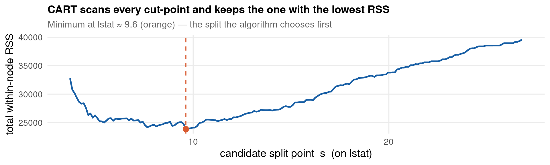
How are the regions chosen? Searching all partitions jointly is infeasible, so CART (Breiman et al. 1984) grows the tree greedily by recursive binary splitting. At each node it picks the variable \(v\) and cut-point \(s\) that most reduce the within-node sum of squares:

\[\min_{v,\,s}\;\Big[\underbrace{\sum_{i:\,x_{iv}\le s}(y_i-\bar y_L)^2}_{\text{left RSS}} \;+\; \underbrace{\sum_{i:\,x_{iv}> s}(y_i-\bar y_R)^2}_{\text{right RSS}}\Big].\]

The objective, in code. A single candidate split’s score is a few lines — this is exactly what rpart/sklearn evaluate internally for every \((v,s)\):

RSS of a candidate split, evaluated on Boston (R)
# RSS if we split variable x at cut-point s (smaller = better split)
split_rss <- function(x, y, s) {
  left  <- y[x <= s];  right <- y[x > s]
  sum((left - mean(left))^2) + sum((right - mean(right))^2)
}
# compare two candidate cut-points on lstat — the lower RSS is the better split
c(split_at_10 = split_rss(boston$lstat, boston$medv, 10),
  split_at_15 = split_rss(boston$lstat, boston$medv, 15))
split_at_10 split_at_15 
   24111.08    27797.71 
RSS of a candidate split, evaluated on Boston (Python)
import pandas as pd
boston = pd.read_csv("../data/boston.csv")
def split_rss(x, y, s):
    left, right = y[x <= s], y[x > s]
    return ((left - left.mean())**2).sum() + ((right - right.mean())**2).sum()
x, y = boston["lstat"], boston["medv"]
print({f"split_at_{s}": round(split_rss(x, y, s), 1) for s in (10, 15)})
{'split_at_10': np.float64(24111.1), 'split_at_15': np.float64(27797.7)}
RSS of a candidate split on Boston (Stata)
import delimited "../data/boston.csv", clear
* RSS at lstat <= 10 : Var*(N-1) is the sum of squared deviations within each side
summarize medv if lstat <= 10
scalar rss = r(Var) * (r(N) - 1)
summarize medv if lstat >  10
scalar rss = rss + r(Var) * (r(N) - 1)
display as text "total within-node RSS at split lstat=10: " as result %9.0f rss
(encoding automatically selected: ISO-8859-1)
(13 vars, 506 obs)

    Variable |        Obs        Mean    Std. dev.       Min        Max
-------------+---------------------------------------------------------
        medv |        219    29.47443    8.910574       11.9         50

    Variable |        Obs        Mean    Std. dev.       Min        Max
-------------+---------------------------------------------------------
        medv |        287    17.23589     4.87689          5         31


total within-node RSS at split lstat=10:     24111

Each split is a two-regime sample-split regression (Hansen 2022, §29.15): \(y = \mu_L\,\mathbf{1}\{x_v\le s\} + \mu_R\,\mathbf{1}\{x_v> s\} + e\). The tree is a step function whose break-points are chosen by the data.

Recursive Partitioning — Why Trees Appeal to Economists

A tree’s mechanics map onto things you already value:

  • Fully non-parametric — captures interactions (\(\text{experience}\times\text{occupation}\)), thresholds, and non-monotonicities with no functional form imposed.
  • No scaling of regressors required; mixed continuous / binary / categorical inputs are handled natively (unlike Lasso, which needs standardised columns).
  • A small tree is interpretable — a sequence of yes/no questions a policy audience can read directly.

Wage example (Causal ML book, Ch. 8). A wage tree first splits on education, then on experience: for college graduates the MSE-minimising experience split is at 9.5 years, for non-graduates at 14 years. The split locations are discovered, and they encode an interaction (the experience cut depends on the education branch) that a linear Mincer equation would have to be told about in advance.

The catch, previewed: this flexibility makes a single tree unstable — a few resampled observations can flip an early split. That instability is what motivates the ensembles of Parts III–IV.

Growing and Pruning — Why Prune at All?

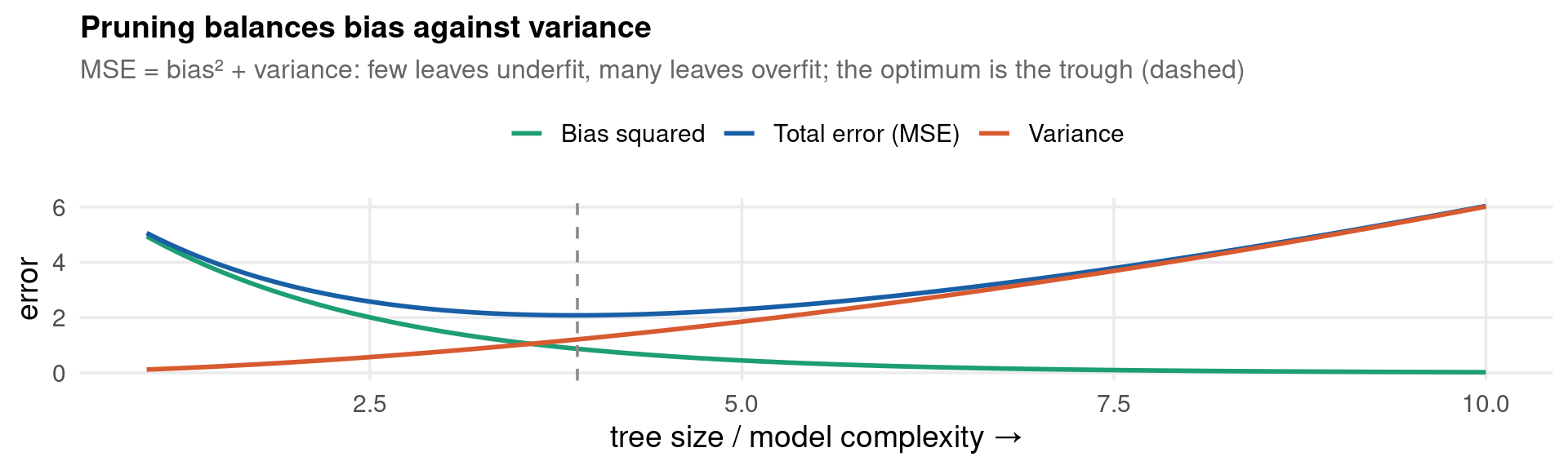
A fully grown tree keeps splitting until each leaf is almost pure. It fits the training data nearly perfectly — and therefore overfits: it has memorised noise that will not repeat out of sample.

The remedy is the same bias–variance trade-off you know from Lasso’s \(\lambda\): grow a large tree, then prune it back to the size that predicts best on held-out data.

  • Too few leaves → high bias (underfit), the step function is too coarse.
  • Too many leaves → high variance (overfit), the steps chase noise.
  • The right size sits at the trough of the cross-validation curve.

The next slide writes this trade-off as a penalised objective; the slide after estimates it on real data.

Growing and Pruning — The Cost-Complexity Objective

Cost-complexity pruning (ISLR §8.1.2; Causal ML Ch. 8) indexes subtrees \(T\) by a penalty \(\alpha\ge 0\) and keeps the subtree minimising training fit plus a per-leaf penalty:

\[R_\alpha(T) = \underbrace{\sum_{\ell\in L(T)}\sum_{i:\,\mathbf{x}_i\in R_\ell}(y_i-\bar y_\ell)^2}_{\text{training RSS } R(T)} \;+\; \alpha\,\lvert L(T)\rvert,\]

where \(\lvert L(T)\rvert\) is the number of leaves. Larger \(\alpha\) ⇒ smaller, more interpretable trees. This is the same shape as a Lasso/Mallows penalty — fit plus a price on complexity. Hansen (2022, §29.16) writes it as \(C = \sum_i \hat e_i^2 + \alpha N\) with \(N\) leaves.

The penalty maps directly onto one argument. In rpart, \(\alpha\) is the complexity parameter cp (scaled by the root error); in sklearn it is ccp_alpha:

Bigger cp = smaller tree (R)
# count leaves at a light vs heavy complexity penalty (cp <-> alpha)
leaves <- function(cp) {
  t <- rpart(medv ~ ., data = boston, method = "anova",
             control = rpart.control(cp = cp, minsplit = 10))
  sum(t$frame$var == "<leaf>")
}
c(cp_0.005 = leaves(0.005), cp_0.05 = leaves(0.05))   # heavier penalty -> fewer leaves
cp_0.005  cp_0.05 
      13        5 
Bigger ccp_alpha = smaller tree (Python)
import pandas as pd
from sklearn.tree import DecisionTreeRegressor
boston = pd.read_csv("../data/boston.csv")
feat = [c for c in boston.columns if c != "medv"]
X = boston[feat].to_numpy(float); y = boston["medv"].to_numpy(float)
for a in (0.0, 2.0):                                   # ccp_alpha <-> alpha
    t = DecisionTreeRegressor(ccp_alpha=a, random_state=SEED).fit(X, y)
    print(f"ccp_alpha={a}: {t.get_n_leaves()} leaves")
ccp_alpha=0.0: 474 leaves
ccp_alpha=2.0: 7 leaves
Forest depth knob via pystacked (Stata)
* Stata has no native CART; the scikit-learn tree behind pystacked carries the same
* complexity knob. Here we just confirm a forest fits and reports its training score.
import delimited "../data/boston.csv", clear
pystacked medv crim zn indus chas nox rm age dis rad tax ptratio lstat, ///
    type(reg) methods(rf) pyseed(14159)
(encoding automatically selected: ISO-8859-1)
(13 vars, 506 obs)

Error loading Python Script for pystacked.
unrecognized command
r(199);

r(199);

Bigger cp/ccp_alpha = heavier penalty = smaller tree. The next slide chooses it by cross-validation.

Growing and Pruning — Choosing \(\alpha\) by Cross-Validation

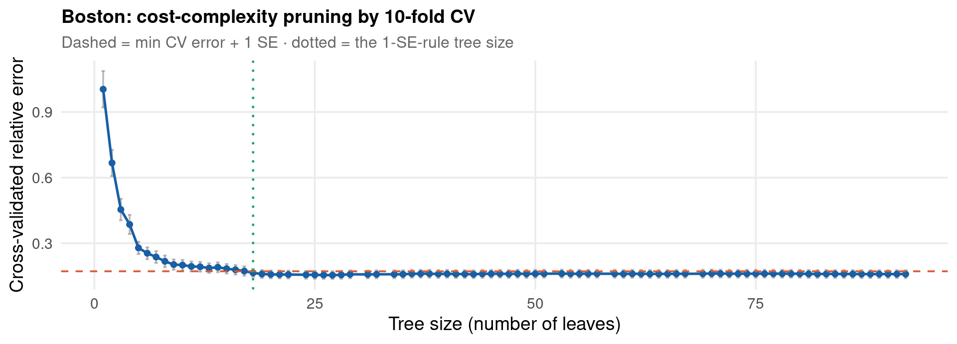
There is no reliable plug-in for \(\alpha\) (unlike some Lasso rules) — cross-validation is the workhorse. We follow the five steps below on Boston.

  1. Data: Boston, 506 tracts, target medv, 12 predictors (all numeric).
  2. Prepare: none needed — trees handle raw scales.
  3. Estimate: grow a deliberately large tree with cp = 0, asking rpart for a 10-fold CV path (xval = 10).
  4. Read: rpart returns a cptable with, per tree size, the CV error xerror and its SE xstd. The 1-SE rule picks the smallest tree within one SE of the minimum.
  5. Plot: CV error against tree size — a U-shape.
Code — cost-complexity pruning on Boston (R)
set.seed(SEED)
# STEP 3 — grow a large tree and read its 10-fold CV pruning path
big_tree <- rpart(medv ~ ., data = boston, method = "anova",
                  control = rpart.control(cp = 0, minsplit = 10, xval = 10))
cpt  <- as_tibble(big_tree$cptable)          # columns: CP, nsplit, rel error, xerror, xstd
# STEP 4 — locate the minimum-CV tree and the 1-SE tree
imin <- which.min(cpt$xerror)
thr  <- cpt$xerror[imin] + cpt$xstd[imin]    # min CV error + 1 SE
i1se <- which(cpt$xerror <= thr)[1]          # smallest tree under that threshold

# STEP 5 — plot CV error vs tree size
ggplot(cpt) +
  aes(nsplit + 1L, xerror) +
  geom_errorbar(aes(ymin = xerror - xstd, ymax = xerror + xstd),
                width = 0.4, colour = col_muted, alpha = 0.6) +
  geom_line(colour = col_main, linewidth = 0.9) +
  geom_point(colour = col_main, size = 1.6) +
  geom_hline(yintercept = thr, linetype = "dashed", colour = col_accent) +
  geom_vline(xintercept = cpt$nsplit[i1se] + 1L, linetype = "dotted",
             colour = col_ok, linewidth = 0.8) +
  labs(x = "Tree size (number of leaves)", y = "Cross-validated relative error",
       title = "Boston: cost-complexity pruning by 10-fold CV",
       subtitle = "Dashed = min CV error + 1 SE · dotted = the 1-SE-rule tree size") +
  theme_lecture

Reading the figure: the curve is U-shaped in tree size. The 1-SE rule (dotted line) picks a parsimonious tree near the trough — the same logic that governed \(\lambda\) for Lasso and Ridge. xerror is relative error (1.0 = a root-only tree), so a value of 0.3 means the tree cut CV error to 30% of the no-split baseline.

Application: the Hitters Tree — Step 1, The Data

We now build the canonical ISLR Figure 8.1 tree: predict a player’s log(Salary) from Years in the majors and Hits last season. First, look at the raw data.

Step 1 — inspect the relevant columns (R)
# How the data looks: 263 players (after dropping missing salaries), salary in $000s
Hitters %>%
  select(Salary, Years, Hits) %>%
  head(6)
                  Salary Years Hits
-Andy Allanson        NA     1   66
-Alan Ashby        475.0    14   81
-Alvin Davis       480.0     3  130
-Andre Dawson      500.0    11  141
-Andres Galarraga   91.5     2   87
-Alfredo Griffin   750.0    11  169
Step 1 — inspect the relevant columns (R)
cat(sprintf("Rows with a salary: %d  |  missing salaries dropped: %d\n",
            sum(!is.na(Hitters$Salary)), sum(is.na(Hitters$Salary))))
Rows with a salary: 263  |  missing salaries dropped: 59

What we see. Salary is in thousands of dollars and is right-skewed (a few stars earn far more) — which is why ISLR models log(Salary). Years and Hits are counts. There are 59 players with a missing salary that we must drop.

Application: the Hitters Tree — Step 2, Prepare

Two preparation steps: drop missing salaries and log-transform the target so the leaves are symmetric in proportional terms.

Step 2 — filter + log-transform (R, tidyverse)
# filter() drops rows; mutate() adds the new log column (never use $ <- here)
hit <- Hitters %>%
  filter(!is.na(Salary)) %>%
  mutate(lsalary = log(Salary))
nrow(hit)
[1] 263

filter(!is.na(Salary)) keeps complete cases; mutate(lsalary = log(Salary)) adds the modelling target.

Step 2 — filter + log-transform (Python, pandas)
import numpy as np, pandas as pd
hit = pd.read_csv("../data/hitters.csv")
hit = hit.dropna(subset=["Salary"]).assign(lsalary=lambda d: np.log(d["Salary"]))
print(len(hit))
263

.dropna(subset=...) ↔︎ filter(!is.na()); .assign(lsalary=...) ↔︎ mutate().

Step 2 — filter + log-transform (Stata)
import delimited "../data/hitters.csv", clear case(lower)
capture drop lsalary
drop if missing(salary)
generate double lsalary = ln(salary)
count
(encoding automatically selected: ISO-8859-1)
(21 vars, 263 obs)


(0 observations deleted)


  263

drop if missing() ↔︎ filter(); generate ↔︎ mutate().

All three end with 263 players and a new lsalary column.

Application: the Hitters Tree — Step 3, Estimate

Now fit the tree. The arguments below are the ones you will tune most often.

Step 3 — fit a small CART tree (R)
set.seed(SEED)
tree_hit <- rpart(lsalary ~ Years + Hits, data = hit, method = "anova",
                  control = rpart.control(maxdepth = 2, cp = 0.01, minbucket = 10))
tree_hit          # printed: the split rules and leaf predictions
n= 263 

node), split, n, deviance, yval
      * denotes terminal node

1) root 263 207.15370 5.927222  
  2) Years< 4.5 90  42.35317 5.106790  
    4) Years< 3.5 62  23.00867 4.891812 *
    5) Years>=3.5 28  10.13439 5.582812 *
  3) Years>=4.5 173  72.70531 6.354036  
    6) Hits< 117.5 90  28.09371 5.998380 *
    7) Hits>=117.5 83  20.88307 6.739687 *
Step 3 — fit a small CART tree (Python)
from sklearn.tree import DecisionTreeRegressor, export_text
Xh = hit[["Years", "Hits"]].to_numpy(dtype=float)
yh = hit["lsalary"].to_numpy(dtype=float)
tree = DecisionTreeRegressor(max_depth=2, min_samples_leaf=10, random_state=SEED).fit(Xh, yh)
print(export_text(tree, feature_names=["Years", "Hits"]))
|--- Years <= 4.50
|   |--- Years <= 3.50
|   |   |--- value: [4.89]
|   |--- Years >  3.50
|   |   |--- value: [5.58]
|--- Years >  4.50
|   |--- Hits <= 117.50
|   |   |--- value: [6.00]
|   |--- Hits >  117.50
|   |   |--- value: [6.74]

Parameters that matter (same idea, three names):

Concept rpart sklearn Effect
Tree depth maxdepth max_depth Caps interaction order; small = readable
Complexity penalty \(\alpha\) cp ccp_alpha Larger ⇒ fewer splits
Min. obs per leaf minbucket min_samples_leaf Larger ⇒ smoother, more regularised
Method method="anova" (regressor) “anova” = regression (RSS) splits

Application: the Hitters Tree — Step 4, Read the Results

A tree’s “coefficients” are its leaf means. Each leaf predicts the average log(Salary) of the players who land in it — the formula \(\bar y_{R_j}\) made concrete.

Step 4 — leaf summaries (R)
# tree_hit$where gives each player's leaf id; group and average within leaf
hit %>%
  mutate(leaf = tree_hit$where) %>%
  group_by(leaf) %>%
  summarise(players       = n(),
            mean_lsalary  = mean(lsalary),
            mean_salary_k = mean(Salary), .groups = "drop") %>%
  arrange(mean_lsalary) %>%
  kbl(caption = "Hitters: terminal-node (leaf) summaries",
      col.names = c("Leaf", "Players", "mean log(Salary)", "mean Salary ($000s)"),
      digits = 2) %>%
  kable_styling(font_size = 20, full_width = TRUE)
Hitters: terminal-node (leaf) summaries
Leaf Players mean log(Salary) mean Salary ($000s)
3 62 4.89 181.37
4 28 5.58 324.29
6 90 6.00 464.92
7 83 6.74 949.17

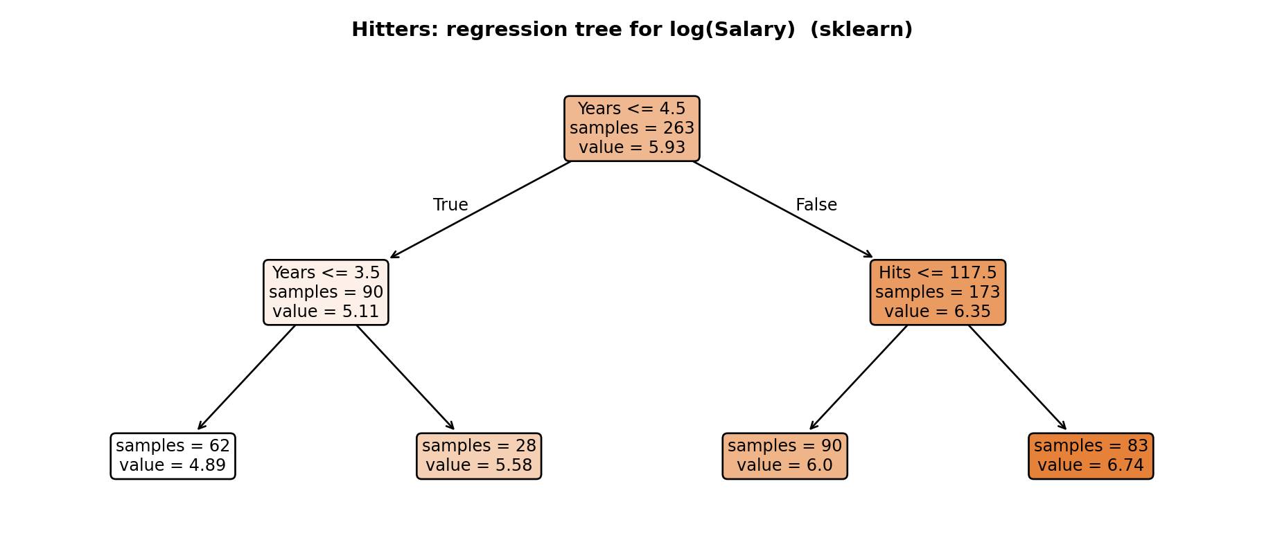
How to read it. Each row is a leaf. The lowest-salary leaf holds inexperienced players (Years < 4.5); among experienced players, more Hits raises predicted salary. The tree has recovered, automatically, that experience matters first and productivity matters mainly once a player is established — an interaction.

Application: the Hitters Tree — Step 5, Plot

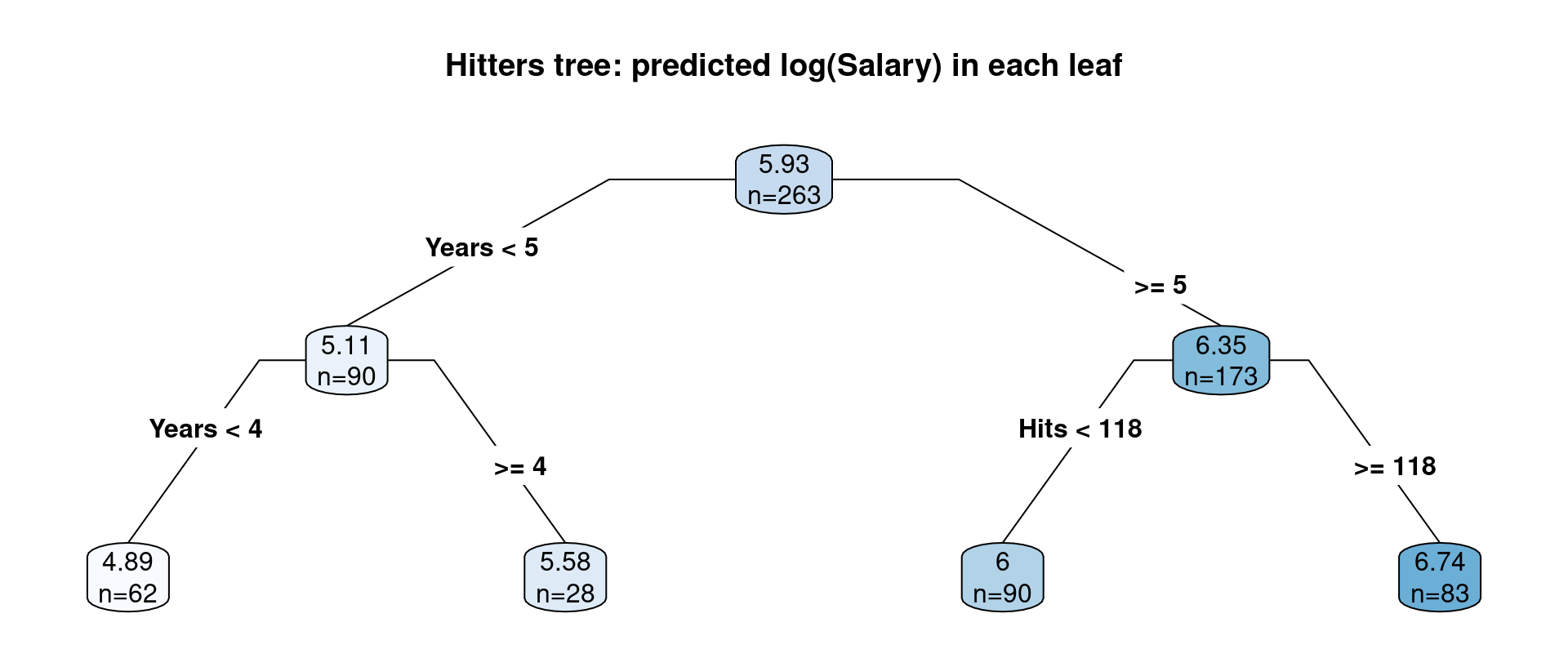
Finally, draw the tree. A tree diagram is the model — the splits are the rules, the leaves are the predictions.

Step 5 — plot the tree (R, rpart.plot)
# type=4 draws split labels on every branch; extra=1 shows n per node
rpart.plot(tree_hit, type = 4, extra = 1, digits = 3, branch = 0.4,
           box.palette = "Blues", fallen.leaves = TRUE,
           main = "Hitters tree: predicted log(Salary) in each leaf")

Step 5 — plot the tree (Python, sklearn)
import matplotlib.pyplot as plt
from sklearn.tree import plot_tree
fig, ax = plt.subplots(figsize=(9.5, 4.2))
# assign the return value to _ so the list of artists is NOT printed
_ = plot_tree(tree, feature_names=["Years", "Hits"], filled=True, rounded=True,
              precision=2, fontsize=9, impurity=False, ax=ax)
_ = ax.set_title("Hitters: regression tree for log(Salary)  (sklearn)",
                 fontsize=11, fontweight="bold")
plt.tight_layout(); plt.show()
Step 5 — a readable tree in Stata
* Stata has no native CART plot. Fit through pystacked and read the rules, or use
* the community command -crtrees-. Here we show the leaf means directly.
import delimited "../data/hitters.csv", clear case(lower)
capture drop lsalary
drop if missing(salary)
generate double lsalary = ln(salary)
* Reproduce the ISLR leaves by hand from the discovered split points:
generate byte leaf = 1 if years < 4.5
replace     leaf = 2 if years >= 4.5 & hits <  117.5
replace     leaf = 3 if years >= 4.5 & hits >= 117.5
table leaf, statistic(mean lsalary) statistic(frequency)
(encoding automatically selected: ISO-8859-1)
(21 vars, 263 obs)


(0 observations deleted)


(173 missing values generated)

(90 real changes made)

(83 real changes made)


-------------------------------
        |      Mean   Frequency
--------+----------------------
leaf    |                      
  1     |   5.10679          90
  2     |   5.99838          90
  3     |  6.739687          83
  Total |  5.927222         263
-------------------------------

Reading the tree (ISLR §8.1.1). Read top to bottom: the first split is Years < 4.5; experienced players are then split at Hits ≈ 117.5. Each leaf box shows its predicted log(Salary).

Decision Trees — The Catch: High Variance

A single tree is interpretable but unstable. Because each split is chosen greedily, a small change in the data can flip an early split and produce a completely different tree below it. In bias–variance terms, a deep tree is low-bias, high-variance.

Property Single decision tree
Bias Low (flexible, non-parametric)
Variance High — unstable to data perturbations
Interpretability High (small trees)
Out-of-sample accuracy Mediocre — variance dominates the error

On Boston, ISLR (§8.3.2) reports a single pruned tree with a test MSE of about 35.3 (\(\text{RMSE}\approx\$5{,}940\)). Part III will cut that by roughly a third — without raising bias.

Two structural disadvantages (Hansen 2022, §29.15). (1) The fit is a discrete step function — crude when the true \(m(\mathbf{x})\) is smooth, so a good fit may need many leaves and high variance. (2) There are no coefficients — nothing to put a standard error on. Ensembles fix (1)’s variance but make interpretability worse; Part V returns to partialling-out to recover an interpretable coefficient.

The cure is aggregation: average many low-bias trees so their variance cancels while their bias stays put — bagging, random forests (Part III), and boosting (Part IV).

Part III — Bagging & Random Forests

“Average many unstable trees, and the noise cancels out.”

Bagging — One Dataset, Many Trees

A single deep tree is (almost) unbiased but high-variance — the regime where, in \(\text{MSE}=\text{bias}^2+\text{variance}\), the variance term dominates.

How do you average many trees when you only have one dataset? You resample it. Bagging (bootstrap aggregating; Breiman 1996) grows \(B\) trees on \(B\) bootstrap resamples and averages their predictions:

\[\hat{f}^{\text{bag}}(\mathbf{x}) = \frac{1}{B}\sum_{b=1}^{B} T_b(\mathbf{x}),\qquad T_b \text{ grown on a size-}n\text{ resample drawn with replacement.}\]

The formula, in code. Bagging by hand is a loop — fit on a resample, store the prediction, average:

Bagging by hand on Boston — average B trees (R)
set.seed(SEED)
n <- nrow(boston); tr <- sample(n, n %/% 2); te <- setdiff(seq_len(n), tr)
B <- 50
preds <- matrix(0, length(te), B)
for (b in seq_len(B)) {
  idx        <- sample(tr, length(tr), replace = TRUE)        # bootstrap resample
  tb         <- rpart(medv ~ ., data = boston[idx, ], method = "anova")
  preds[, b] <- predict(tb, boston[te, ])                     # store its predictions
}
single <- predict(rpart(medv ~ ., data = boston[tr, ]), boston[te, ])
c(one_tree_MSE   = mean((single          - boston$medv[te])^2),
  bagged_B50_MSE = mean((rowMeans(preds) - boston$medv[te])^2))   # averaging cuts variance
  one_tree_MSE bagged_B50_MSE 
      26.53701       22.19169 
Bagging by hand on Boston (Python)
import pandas as pd, numpy as np
from sklearn.tree import DecisionTreeRegressor
from sklearn.model_selection import train_test_split
from sklearn.metrics import mean_squared_error
boston = pd.read_csv("../data/boston.csv")
feat = [c for c in boston.columns if c != "medv"]
X = boston[feat].to_numpy(float); y = boston["medv"].to_numpy(float)
Xtr, Xte, ytr, yte = train_test_split(X, y, test_size=0.5, random_state=SEED)
B = 50; rng = np.random.default_rng(SEED)
preds = np.zeros((len(Xte), B))
for b in range(B):
    idx = rng.integers(0, len(Xtr), len(Xtr))                # bootstrap resample
    preds[:, b] = DecisionTreeRegressor(random_state=b).fit(Xtr[idx], ytr[idx]).predict(Xte)
single = DecisionTreeRegressor(random_state=SEED).fit(Xtr, ytr).predict(Xte)
print(f"one tree MSE: {mean_squared_error(yte, single):.2f} | "
      f"bagged (B=50) MSE: {mean_squared_error(yte, preds.mean(1)):.2f}")
The bagging loop, done for you by pystacked (Stata)
* `bsample` is Stata's bootstrap-resample primitive; a random forest IS bagged trees,
* so pystacked wraps the whole loop into one call:
import delimited "../data/boston.csv", clear
pystacked medv crim zn indus chas nox rm age dis rad tax ptratio lstat, ///
    type(reg) methods(rf) pyseed(14159)
(encoding automatically selected: ISO-8859-1)
(13 vars, 506 obs)

Error loading Python Script for pystacked.
unrecognized command
r(199);

r(199);

In practice ranger (R), RandomForestRegressor (Python), or pystacked (Stata) does this loop for you, in parallel and in C++.

Bagging — Out-of-Bag Error for Free

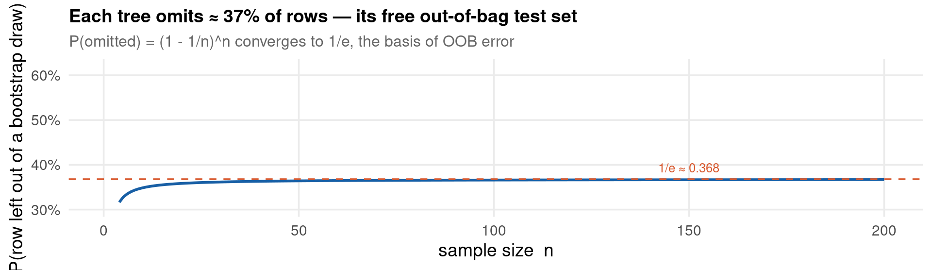
How do you estimate test error without a test set? Use the observations each tree did not see. A bootstrap resample omits on average \(\approx 1/e \approx 37\%\) of the rows — the out-of-bag (OOB) sample. Predict each \(\mathbf{x}_i\) using only the trees that excluded it:

\[\hat{f}^{\text{OOB}}(\mathbf{x}_i)=\frac{1}{|\{b:\,i\notin b\}|}\sum_{b:\,i\notin b} T_b(\mathbf{x}_i).\]

The OOB MSE approximates leave-one-out cross-validation at no extra cost. In code it is a single argument or attribute:

OOB error on Boston, computed automatically (R)
set.seed(SEED)
rf <- ranger(medv ~ ., data = boston, num.trees = N_TREES,
             num.threads = N_THREADS, seed = SEED)
rf$prediction.error              # OOB MSE — a free held-out estimate, no test split
[1] 10.61716
OOB error on Boston (Python)
import pandas as pd
from sklearn.ensemble import RandomForestRegressor
from sklearn.metrics import mean_squared_error
boston = pd.read_csv("../data/boston.csv")
feat = [c for c in boston.columns if c != "medv"]
X = boston[feat].to_numpy(float); y = boston["medv"].to_numpy(float)
rf = RandomForestRegressor(n_estimators=N_TREES, oob_score=True,
                           n_jobs=N_CORES, random_state=SEED).fit(X, y)
print(f"OOB MSE: {mean_squared_error(y, rf.oob_prediction_):.2f}")
OOB scoring requested from pystacked (Stata)
import delimited "../data/boston.csv", clear
* the scikit-learn forest behind pystacked computes the out-of-bag fit
pystacked medv crim zn indus chas nox rm age dis rad tax ptratio lstat, ///
    type(reg) methods(rf) cmdopt1(oob_score(True)) pyseed(14159)
(encoding automatically selected: ISO-8859-1)
(13 vars, 506 obs)

Error loading Python Script for pystacked.
unrecognized command
r(199);

r(199);

We exploit exactly these OOB predictions as a cheap cross-fitting device in Part V — the bridge from prediction to inference. References: Breiman (1996, 2001); Hansen §29.16; Causal ML Ch. 8.

Random Forests — Why Bagging Is Not Enough

If averaging is so powerful, why not stop at bagging? Because the trees are correlated. If one predictor dominates — lstat in Boston — almost every bootstrapped tree splits on it first, so the trees look alike and their errors do not cancel.

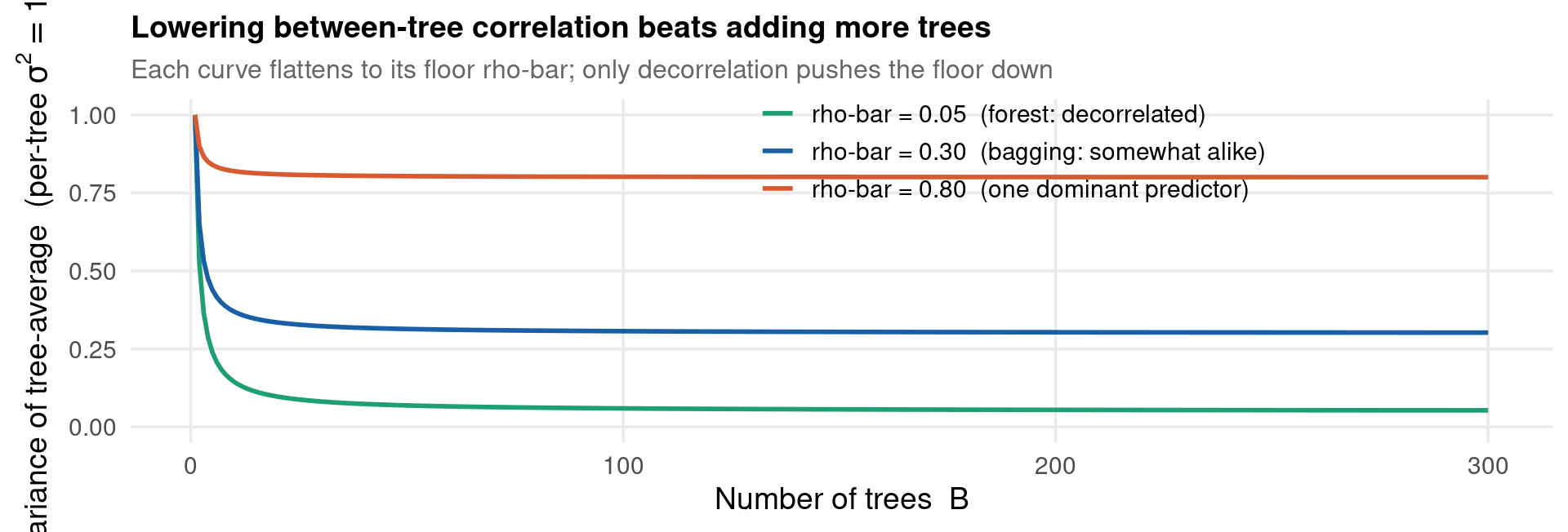
Write the variance of the average via the per-tree variance \(\sigma^2\) and the average pairwise correlation \(\bar\rho\):

\[\operatorname{Var}\!\Big(\tfrac{1}{B}\textstyle\sum_{b=1}^B T_b\Big) = \bar\rho\,\sigma^2 + \frac{1-\bar\rho}{B}\,\sigma^2 \;\xrightarrow{\;B\to\infty\;}\;\bar\rho\,\sigma^2.\]

The second term vanishes as \(B\) grows — but the first does not. The variance floor is \(\bar\rho\,\sigma^2\). Adding trees buys you only the second term; to break through the floor you must lower \(\bar\rho\).

Code — the variance formula, plotted (not a simulation)
# This plots the algebra Var = rho + (1-rho)/B (with sigma^2 = 1), NOT data.
var_curve <- function(rho) tibble(B = 1:300, variance = rho + (1 - rho) / (1:300), rho = rho)
var_df <- bind_rows(var_curve(0.05), var_curve(0.30), var_curve(0.80)) %>%
  mutate(label = factor(rho, levels = c(0.05, 0.30, 0.80),
                        labels = c("rho-bar = 0.05  (forest: decorrelated)",
                                   "rho-bar = 0.30  (bagging: somewhat alike)",
                                   "rho-bar = 0.80  (one dominant predictor)")))
ggplot(var_df) +
  aes(B, variance, colour = label) +
  geom_line(linewidth = 1) +
  scale_colour_manual(values = c(col_ok, col_main, col_accent)) +
  scale_y_continuous(limits = c(0, 1)) +
  labs(x = "Number of trees  B", colour = NULL,
       y = expression("Variance of tree-average  (per-tree "*sigma^2 == 1*")"),
       title = "Lowering between-tree correlation beats adding more trees",
       subtitle = "Each curve flattens to its floor rho-bar; only decorrelation pushes the floor down") +
  theme_lecture +
  theme(legend.position = c(0.62, 0.85))

Past a few hundred trees, more trees barely help — what helps is making the trees different from each other.

Random Forests — The Second Randomisation

How does a forest make its trees different? It restricts the competition at every split: a random subset of \(m\le p\) predictors is considered as candidates at each node (Breiman 2001).

Source of randomness What it reduces Mechanism
Bootstrap resampling (bagging) Variance across observations Each tree fits a different resample
Feature subsampling (\(m<p\)) Correlation \(\bar\rho\) between trees Each split sees a different feature subset

With \(m<p\), a tree is sometimes forced to ignore the dominant predictor and find structure elsewhere — so the trees disagree, \(\bar\rho\) falls, and the variance floor drops.

The one knob worth tuning is \(m\) (mtry / max_features). Conventional defaults (ISLR §8.2.2):

Setting Regression Classification
Default \(m\) \(\lfloor p/3 \rfloor\) \(\lfloor \sqrt{p} \rfloor\)
Bagging \(m=p\) (all predictors) \(m=p\)
Forest (m = p/3) vs bagging (m = p) by OOB error (R)
set.seed(SEED)
p <- ncol(boston) - 1L
forest <- ranger(medv ~ ., data = boston, mtry = floor(p / 3),
                 num.trees = N_TREES, num.threads = N_THREADS, seed = SEED)
bagging <- ranger(medv ~ ., data = boston, mtry = p,
                  num.trees = N_TREES, num.threads = N_THREADS, seed = SEED)
c(forest_mtry_p3 = forest$prediction.error, bagging_mtry_p = bagging$prediction.error)
forest_mtry_p3 bagging_mtry_p 
      9.952539      10.589796 
Forest vs bagging by OOB error (Python)
import pandas as pd
from sklearn.ensemble import RandomForestRegressor
from sklearn.metrics import mean_squared_error
boston = pd.read_csv("../data/boston.csv")
feat = [c for c in boston.columns if c != "medv"]
X = boston[feat].to_numpy(float); y = boston["medv"].to_numpy(float); p = X.shape[1]
for m, name in [(max(1, p // 3), "forest (m=p/3)"), (p, "bagging (m=p)")]:
    rf = RandomForestRegressor(n_estimators=N_TREES, max_features=m, oob_score=True,
                               n_jobs=N_CORES, random_state=SEED).fit(X, y)
    print(f"{name}: OOB MSE = {mean_squared_error(y, rf.oob_prediction_):.2f}")
Set max_features via pystacked (Stata)
import delimited "../data/boston.csv", clear
* forest restricts the per-split feature subset; bagging uses all 12
pystacked medv crim zn indus chas nox rm age dis rad tax ptratio lstat, ///
    type(reg) methods(rf) cmdopt1(max_features(4)) pyseed(14159)
(encoding automatically selected: ISO-8859-1)
(13 vars, 506 obs)

Error loading Python Script for pystacked.
unrecognized command
r(199);

r(199);

What to tune (and what not to). num.trees/n_estimators: set it large (500–1000) — more is never worse, only slower; do not “tune” it. mtry: the key knob, tune by OOB error around \(p/3\). min.node.size/min_samples_leaf: larger = more regularisation (5 is a common regression default). A forest is far more forgiving than the boosting of Part IV.

Random Forests — Which Variables Matter?

A forest is hundreds of trees. Can it still tell us which predictors it used? Yes — via variable importance, with two measures.

① Impurity (mean decrease in node impurity). Sum, over all splits on \(x_j\), the reduction in within-node RSS. Cheap (a by-product of fitting) but biased toward continuous / high-cardinality predictors — they offer more candidate split points, so they can rank high even as noise. Treat with suspicion.

② Permutation (mean decrease in accuracy) — preferred. Permute \(x_j\) in the OOB sample, breaking its link with \(y\), and measure how much OOB error rises:

\[\text{VI}_j^{\text{perm}} = \overline{\text{err}}_{\text{OOB, }x_j\text{ permuted}} - \overline{\text{err}}_{\text{OOB}}.\]

Because it is computed out-of-bag, it is an honest out-of-sample measure. In code it is one argument (R) or one function (Python):

Permutation importance on Boston, top predictors (R)
set.seed(SEED)
rf <- ranger(medv ~ ., data = boston, num.trees = N_TREES, importance = "permutation",
             num.threads = N_THREADS, seed = SEED)
sort(rf$variable.importance, decreasing = TRUE)[1:5]   # the predictors the forest leans on
    lstat        rm     indus       nox      crim 
54.317300 31.004658 11.500527  9.683462  9.167599 
Permutation importance on Boston (Python)
import pandas as pd, numpy as np
from sklearn.ensemble import RandomForestRegressor
from sklearn.inspection import permutation_importance
boston = pd.read_csv("../data/boston.csv")
feat = [c for c in boston.columns if c != "medv"]
X = boston[feat].to_numpy(float); y = boston["medv"].to_numpy(float)
rf = RandomForestRegressor(n_estimators=N_TREES, n_jobs=N_CORES,
                           random_state=SEED).fit(X, y)
imp = permutation_importance(rf, X, y, n_repeats=10, random_state=SEED).importances_mean
print(pd.Series(imp, index=feat).sort_values(ascending=False).head(5).round(2))
Fit the forest; importances live in the sklearn object (Stata)
* No native permutation-importance command; fit with pystacked, then read
* feature_importances_ from the underlying scikit-learn object via the Python link.
import delimited "../data/boston.csv", clear
pystacked medv crim zn indus chas nox rm age dis rad tax ptratio lstat, ///
    type(reg) methods(rf) pyseed(14159)
(encoding automatically selected: ISO-8859-1)
(13 vars, 506 obs)

Error loading Python Script for pystacked.
unrecognized command
r(199);

r(199);

A high-importance variable is not a causal effect. A variable can rank high because it is correlated with a true driver; with two correlated predictors a forest may split the credit arbitrarily. Use importance for screening — which controls deserve a structural look — never as evidence of a causal effect. For causal targets, go to Part V.

Application: Boston — Step 1–2, Data and the Train/Test Split

Does decorrelating the trees actually lower test error? We answer on Boston, reproducing ISLR Lab §8.3.3: predict medv from all 12 predictors.

  • Data: 506 census tracts; target medv (median home value, $000s); 12 numeric predictors. Two dominate: lstat (% lower-status population) and rm (rooms/dwelling).
  • Prepare: trees need no scaling. The only step is an honest train/test split — fit on one half, measure error on the other, so we never grade the model on data it has seen.
set.seed(SEED)                          # reproducible split
train <- sample(nrow(boston), nrow(boston) / 2)   # half the row indices
# boston[train, ] -> fit;  boston[-train, ] -> evaluate
from sklearn.model_selection import train_test_split
Xtr, Xte, ytr, yte = train_test_split(X, y, test_size=0.5, random_state=SEED)
set seed 14159
generate byte train = runiform() < 0.5     // ~half the rows flagged for fitting
* estimate "if train", evaluate "if !train"

The seed makes the split reproducible; sharing it across R/Python/Stata keeps the numbers comparable. ISLR’s benchmark on this split: single tree \(\approx 35.3\), bagging \(\approx 23.4\), forest lower still.

Application: Boston — Step 3–4, Estimate and Read

Fit three models that differ only in mtry: a single tree, bagging (\(m=p\)), and a forest (\(m=p/3\)). Reading the test-MSE column shows the variance-floor argument made concrete.

Estimate tree / bagging / forest + read test MSE (R)
set.seed(SEED)
n      <- nrow(boston)
train  <- sample(n, floor(n / 2))
y_test <- boston$medv[-train]
p      <- ncol(boston) - 1L                        # 12 predictors

fit_tree <- rpart(medv ~ ., data = boston[train, ], method = "anova",
                  control = rpart.control(cp = 0.01, xval = 10))
mse_tree <- mean((predict(fit_tree, boston[-train, ]) - y_test)^2)

fit_bag <- ranger(medv ~ ., data = boston[train, ], num.trees = N_TREES,
                  mtry = p, num.threads = N_THREADS, seed = SEED)              # bagging: mtry = p
mse_bag <- mean((predict(fit_bag, boston[-train, ])$predictions - y_test)^2)

fit_rf <- ranger(medv ~ ., data = boston[train, ], num.trees = N_TREES,
                 mtry = floor(p / 3), importance = "permutation",
                 num.threads = N_THREADS, seed = SEED)                         # forest: mtry = p/3
mse_rf <- mean((predict(fit_rf, boston[-train, ])$predictions - y_test)^2)

tibble(Method      = c("Single pruned tree", "Bagging  (mtry = p)", "Random forest  (mtry = p/3)"),
       `Test MSE`  = c(mse_tree, mse_bag, mse_rf),
       `Test RMSE` = sqrt(c(mse_tree, mse_bag, mse_rf)),
       mtry        = c(NA_integer_, p, as.integer(floor(p / 3)))) %>%
  kbl(caption = "Boston: test error, 50/50 split (ISLR §8.3: tree ~35.3, bagging ~23.4, RF lower)",
      digits = 2) %>%
  kable_styling(font_size = 19, full_width = TRUE) %>%
  row_spec(3, bold = TRUE, color = "white", background = col_main)
Boston: test error, 50/50 split (ISLR §8.3: tree ~35.3, bagging ~23.4, RF lower)
Method Test MSE Test RMSE mtry
Single pruned tree 26.54 5.15 NA
Bagging (mtry = p) 15.49 3.94 12
Random forest (mtry = p/3) 16.07 4.01 4
Estimate tree / bagging / forest + read test MSE (Python)
import pandas as pd, numpy as np
from sklearn.tree import DecisionTreeRegressor
from sklearn.ensemble import RandomForestRegressor
from sklearn.model_selection import train_test_split
from sklearn.metrics import mean_squared_error

boston = pd.read_csv("../data/boston.csv")
feat = [c for c in boston.columns if c != "medv"]
X = boston[feat].to_numpy(dtype=float)
y = boston["medv"].to_numpy(dtype=float)
p = X.shape[1]
Xtr, Xte, ytr, yte = train_test_split(X, y, test_size=0.5, random_state=SEED)

tree = DecisionTreeRegressor(min_samples_leaf=5, random_state=SEED).fit(Xtr, ytr)
bag  = RandomForestRegressor(n_estimators=N_TREES, max_features=p,
                             n_jobs=N_CORES, random_state=SEED).fit(Xtr, ytr)   # bagging
rf   = RandomForestRegressor(n_estimators=N_TREES, max_features=max(1, p // 3),
                             n_jobs=N_CORES, random_state=SEED).fit(Xtr, ytr)   # forest

mse = lambda m: mean_squared_error(yte, m.predict(Xte))
print(f"Test MSE  — single tree: {mse(tree):.2f} | bagging: {mse(bag):.2f} "
      f"| random forest: {mse(rf):.2f}")
Random forest via pystacked (Stata)
* pystacked (Ahrens, Hansen & Schaffer 2023) wraps scikit-learn, so the numbers
* track the Python tab. Needs: ssc install pystacked  (+ Stata's Python link)
import delimited "../data/boston.csv", clear
set seed 14159
generate byte train = runiform() < 0.5            // 50/50 split, as in R/Python

pystacked medv crim zn indus chas nox rm age dis rad tax ptratio lstat ///
    if train, type(reg) methods(rf) pyseed(14159)

predict double mhat
generate double sq_err = (medv - mhat)^2 if !train
quietly summarize sq_err if !train
display as text "Random-forest test MSE (Stata/pystacked): " as result %6.2f r(mean)
(encoding automatically selected: ISO-8859-1)
(13 vars, 506 obs)


Error loading Python Script for pystacked.
unrecognized command
r(199);

r(199);

Reading the result. Bagging cuts the single-tree MSE by roughly a third; the forest (\(m=p/3\)) lowers it further by decorrelating the trees — precisely the variance-floor argument. The only thing that changed between bagging and the forest is mtry.

Application: Boston — Step 5, Variable Importance Plot

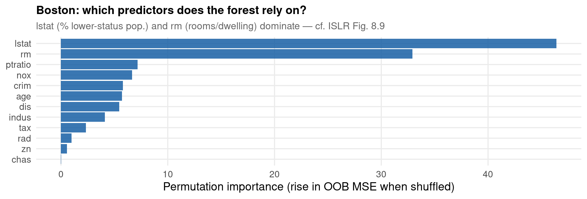
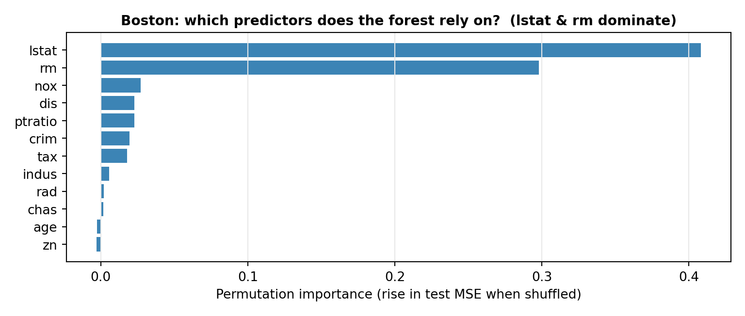
Which predictors does the forest lean on? We plot permutation importance (the honest measure).

Plot permutation importance (R)
tibble(Variable   = names(fit_rf$variable.importance),
       Importance = fit_rf$variable.importance) %>%
  ggplot() +
    aes(reorder(Variable, Importance), Importance) +
  geom_col(fill = col_main, alpha = 0.85) +
  coord_flip() +
  labs(x = NULL, y = "Permutation importance (rise in OOB MSE when shuffled)",
       title = "Boston: which predictors does the forest rely on?",
       subtitle = "lstat (% lower-status pop.) and rm (rooms/dwelling) dominate — cf. ISLR Fig. 8.9") +
  theme_lecture
Plot permutation importance (Python)
import matplotlib.pyplot as plt
from sklearn.inspection import permutation_importance

perm  = permutation_importance(rf, Xte, yte, n_repeats=10,
                               random_state=SEED, n_jobs=N_CORES)
order = np.argsort(perm.importances_mean)[::-1]
fig, ax = plt.subplots(figsize=(8, 3.4))
_ = ax.barh([feat[i] for i in order[::-1]], perm.importances_mean[order[::-1]],
            color="#1a6ea8", alpha=0.85)
_ = ax.set_xlabel("Permutation importance (rise in test MSE when shuffled)")
_ = ax.set_title("Boston: which predictors does the forest rely on?  (lstat & rm dominate)",
                 fontsize=10.5, fontweight="bold")
ax.grid(True, axis="x", color="#e8e8e8")
plt.tight_layout(); plt.show()
Drop-column importance (Stata, pystacked)
* No native permutation importance in Stata. A clean, runnable analogue is
* leave-one-covariate-out (drop-column) importance: refit without each predictor
* and measure the rise in held-out MSE. Needs: ssc install pystacked
import delimited "../data/boston.csv", clear
set seed 14159
generate byte train = runiform() < 0.5
local X crim zn indus chas nox rm age dis rad tax ptratio lstat

* baseline forest and its held-out MSE
quietly pystacked medv `X' if train, type(reg) methods(rf) pyseed(14159)
predict double f_all
quietly generate double e_all = (medv - f_all)^2 if !train
quietly summarize e_all if !train
scalar mse_all = r(mean)

* refit dropping each predictor in turn; a larger MSE rise = more important
foreach v of local X {
    local rest : list X - v
    quietly pystacked medv `rest' if train, type(reg) methods(rf) pyseed(14159)
    quietly predict double f_`v'
    quietly generate double e_`v' = (medv - f_`v')^2 if !train
    quietly summarize e_`v' if !train
    display as text "`v': drop-column importance = " as result %6.3f (r(mean) - mse_all)
}
(encoding automatically selected: ISO-8859-1)
(13 vars, 506 obs)


unrecognized command
r(199);

r(199);

Across all three languages, lstat and rm are the two predictors the forest leans on most — consistent with economic intuition (neighbourhood wealth and dwelling size). The Stata tab uses a drop-column measure (refit-without-each-variable) rather than permutation, so with correlated predictors the two can disagree on the smaller variables — but the top of the ranking is robust.

Part IV — Gradient Boosting & XGBoost

“Each new tree fixes what the last one got wrong.”

Gradient Boosting — Learning From Mistakes

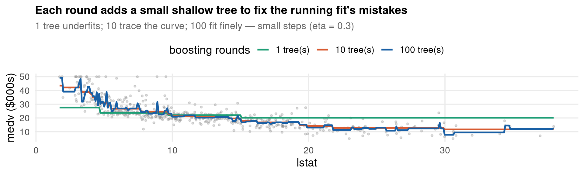
A forest grows trees independently and averages them. What if, instead, each new tree focused on the errors the current model still makes? That is boosting (Friedman 2001): an additive model built sequentially,

\[\hat{f}^{(m)}(\mathbf{x}) = \hat{f}^{(m-1)}(\mathbf{x}) + \nu\,T_m(\mathbf{x}),\]

where \(T_m\) is a shallow tree fit to the negative gradient of the loss (for squared error, the current residuals) and \(\nu\in(0,1)\) is a learning rate taking small steps so no single tree dominates.

The formula, in code. Plain gradient boosting for squared-error loss is a short loop — fit a stump to the residuals, take a small step, update:

Gradient boosting by hand on Boston (R)
y     <- boston$medv
preds <- boston %>% select(-medv)              # the predictor columns
f_hat <- rep(mean(y), length(y)); nu <- 0.1    # start at the mean; small learning rate
for (m in 1:50) {
  d     <- preds %>% mutate(r = y - f_hat)     # current residuals = neg. gradient
  stump <- rpart(r ~ ., data = d, control = rpart.control(maxdepth = 2))
  f_hat <- f_hat + nu * predict(stump, d)      # small step in the residual's direction
}
c(start_RMSE   = sqrt(mean((y - mean(y))^2)),
  boosted_RMSE = sqrt(mean((y - f_hat)^2)))    # training error falls as trees are added
  start_RMSE boosted_RMSE 
    9.188012     2.779872 
Gradient boosting by hand on Boston (Python)
import pandas as pd, numpy as np
from sklearn.tree import DecisionTreeRegressor
boston = pd.read_csv("../data/boston.csv")
feat = [c for c in boston.columns if c != "medv"]
X = boston[feat].to_numpy(float); y = boston["medv"].to_numpy(float)
f_hat = np.full(len(y), y.mean()); nu = 0.1    # start at the mean; small learning rate
for m in range(50):
    r = y - f_hat                              # current residuals = neg. gradient
    stump = DecisionTreeRegressor(max_depth=2).fit(X, r)
    f_hat += nu * stump.predict(X)             # small step in the residual's direction
print(f"start RMSE: {np.sqrt(((y - y.mean())**2).mean()):.2f} | "
      f"boosted RMSE: {np.sqrt(((y - f_hat)**2).mean()):.2f}")
The same loop, done for you by pystacked’s gradient boosting (Stata)
import delimited "../data/boston.csv", clear
pystacked medv crim zn indus chas nox rm age dis rad tax ptratio lstat, ///
    type(reg) methods(gradboost) cmdopt1(learning_rate(0.1) max_depth(2) n_estimators(50)) ///
    pyseed(14159)
(encoding automatically selected: ISO-8859-1)
(13 vars, 506 obs)

Error loading Python Script for pystacked.
unrecognized command
r(199);

r(199);

xgboost (R/Python) and pystacked’s gradboost (Stata) do this loop with a second-order step and regularisation — but the skeleton above is the algorithm.

Gradient Boosting — Forest vs Boosting

Why does sequential fitting work where a single tree fails? A single deep tree is low-bias/high-variance. Boosting goes the other way: it combines many high-bias, low-variance stumps, each chipping at the remaining bias, with variance held down by the small step \(\nu\) and shallow depth.

Random forest Gradient boosting
Trees built In parallel, independently Sequentially, each on the last residual
Each tree Deep (low bias, high variance) Shallow (high bias, low variance)
Variance controlled by Averaging decorrelated trees Small learning rate \(\nu\), shallow depth
Bias controlled by Deep trees Adding more rounds
Overfits if you add trees? No (averaging is safe) Yes — must stop early
Hyperparameters Few, forgiving Many, interacting

The critical contrast. More trees never hurt a forest, but they will eventually overfit a boosted model. Boosting trades robustness for accuracy — and demands more care (early stopping, next slides).

XGBoost — Boosting Meets Regularisation

XGBoost (Chen & Guestrin 2016) dominates applied prediction on tabular data. At each round it minimises a regularised objective:

\[\mathcal{L}^{(m)} = \sum_{i=1}^{n}\ell\!\big(y_i,\,\hat f^{(m-1)}(\mathbf{x}_i)+T_m(\mathbf{x}_i)\big) + \Omega(T_m), \qquad \Omega(T) = \gamma\,\lvert L(T)\rvert + \tfrac{\lambda}{2}\lVert \mathbf{w}\rVert_2^2 + \alpha\lVert \mathbf{w}\rVert_1.\]

Where have you seen \(\lVert\mathbf{w}\rVert_2^2\) and \(\lVert\mathbf{w}\rVert_1\) before? In Ridge and Lasso. XGBoost puts exactly those penalties on the leaf weights \(\mathbf{w}\). The companion deck’s penalties reappear here, one level down — and they map straight onto arguments:

Penalty term Role xgboost argument Companion-deck analogue
\(\tfrac{\lambda}{2}\lVert\mathbf{w}\rVert_2^2\) \(\ell_2\) shrinkage of leaf values lambda (R) / reg_lambda (Py) Ridge
\(\alpha\lVert\mathbf{w}\rVert_1\) \(\ell_1\) sparsity of leaf values alpha / reg_alpha Lasso
\(\gamma\lvert L(T)\rvert\) price per leaf gamma cost-complexity pruning

What XGBoost adds beyond textbook boosting: a second-order (Newton) step; row/column subsampling (subsample, colsample_bytree) borrowing the forest’s decorrelation trick; and efficient handling of missing/sparse inputs. In one object: boosting + Ridge + Lasso + forest-style subsampling — powerful, and easy to overfit.

XGBoost — Hyperparameters and Early Stopping

With so many knobs, how do you avoid overfitting? The single most important discipline is early stopping: watch a validation metric and stop when it stops improving.

Parameter Role Typical range Guidance
eta / learning_rate \(\nu\) Step size per round 0.01–0.3 Smaller is safer; compensate with more rounds
nrounds / n_estimators Max rounds 100–5000 Do not tune by hand — let early stopping choose
max_depth Tree depth 3–6 Start at 3; deeper = more interactions, more overfit
subsample Row subsampling 0.5–1.0 0.8 is a sensible default
colsample_bytree Feature subsampling 0.3–1.0 Mirrors a forest’s mtry
lambda / alpha \(\ell_2\) / \(\ell_1\) leaf penalties 0–10 / 0–1 Ridge/Lasso shrinkage on leaves

Early stopping, in code. Hold out a validation set, watch its RMSE, halt after it fails to improve for, say, 30 rounds — this simultaneously prevents overfitting and selects n_estimators:

xgb.train(params, dtrain, nrounds = 1000,
          evals = list(train = dtrain, test = dtest),   # 'evals' (xgboost >= 2.1; was 'watchlist')
          early_stopping_rounds = 30)        # stop if test RMSE stalls for 30 rounds
XGBRegressor(n_estimators=1000, early_stopping_rounds=30, eval_metric="rmse")
# then: model.fit(Xtr, ytr, eval_set=[(Xte, yte)])
* pystacked passes early stopping straight to the scikit-learn back-end:
pystacked y x*, type(reg) methods(gradboost) ///
    cmdopt1(n_iter_no_change(30) validation_fraction(0.2) learning_rate(0.05))

Application: Boston XGBoost — Estimate With Early Stopping

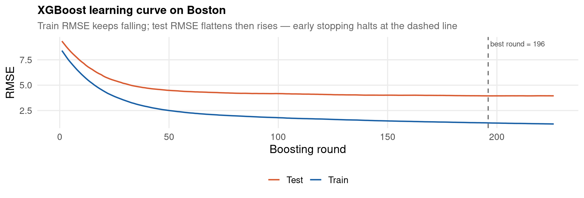
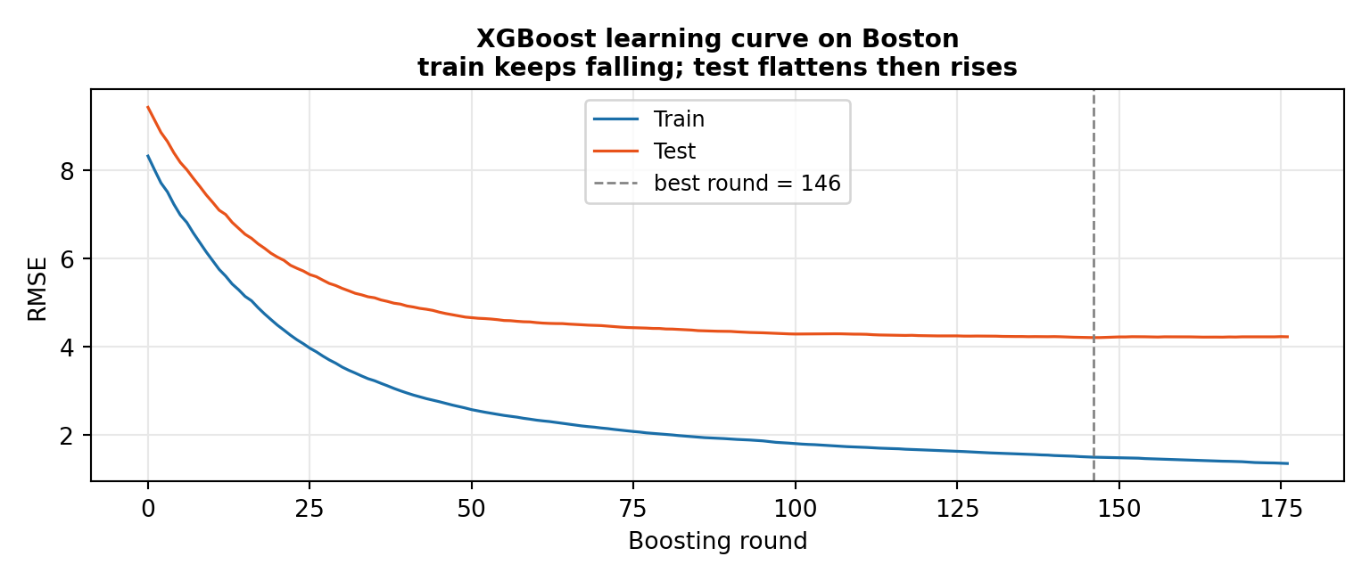
Same Boston train/test split. We fit XGBoost with a small eta, a depth-3 base learner, and early stopping, then read the round at which the held-out error stopped improving.

Fit XGBoost + read best round (R)
set.seed(SEED)
xvars  <- setdiff(names(boston), "medv")
n      <- nrow(boston); train <- sample(n, floor(n / 2))
Xtr    <- as.matrix(boston[train,  xvars]); ytr <- boston$medv[train]
Xte    <- as.matrix(boston[-train, xvars]); yte <- boston$medv[-train]
dtrain <- xgb.DMatrix(Xtr, label = ytr)            # XGBoost's native data container
dtest  <- xgb.DMatrix(Xte, label = yte)

params <- list(objective = "reg:squarederror", max_depth = 3, eta = 0.05,
               subsample = 0.8, colsample_bytree = 0.8, lambda = 1)
fit_xgb <- xgb.train(params, dtrain, nrounds = 1000,
                     evals = list(train = dtrain, test = dtest),  # 'evals' replaces 'watchlist' (xgboost >= 2.1)
                     early_stopping_rounds = 30, verbose = 0)
mse_xgb <- mean((predict(fit_xgb, dtest) - yte)^2)
# In xgboost >= 2.1 the booster is an altrep object; read the log from R attributes
# and take the best round from the log itself (robust to API changes).
elog    <- as_tibble(attributes(fit_xgb)$evaluation_log)
best_it <- elog$iter[which.min(elog$test_rmse)]     # round with the lowest held-out RMSE
cat(sprintf("XGBoost: test MSE %.2f (RMSE %.2f) at %d rounds\n",
            mse_xgb, sqrt(mse_xgb), best_it))
XGBoost: test MSE 15.55 (RMSE 3.94) at 196 rounds
Fit XGBoost + read best round (R)
# Learning curve: train vs test RMSE per round (tidy reshape, no $ assigns)
eval_long <- elog %>%
  pivot_longer(c(train_rmse, test_rmse), names_to = "set", values_to = "rmse") %>%
  mutate(set = recode(set, train_rmse = "Train", test_rmse = "Test"))
ggplot(eval_long) +
  aes(x = iter, y = rmse, colour = set) +
  geom_line(linewidth = 0.8) +
  geom_vline(xintercept = best_it, linetype = "dashed", colour = "grey40") +
  annotate("text", x = best_it, y = max(eval_long$rmse),
           label = paste0(" best round = ", best_it),
           hjust = 0, vjust = 1, size = 3.2, colour = "grey30") +
  scale_colour_manual(values = c(Train = col_main, Test = col_accent)) +
  labs(x = "Boosting round", y = "RMSE", colour = NULL,
       title = "XGBoost learning curve on Boston",
       subtitle = "Train RMSE keeps falling; test RMSE flattens then rises — early stopping halts at the dashed line") +
  theme_lecture
Fit XGBoost + read best round (Python)
import pandas as pd, numpy as np, matplotlib.pyplot as plt
import xgboost as xgb
from sklearn.model_selection import train_test_split

boston = pd.read_csv("../data/boston.csv")
feat = [c for c in boston.columns if c != "medv"]
X = boston[feat].to_numpy(dtype=float); y = boston["medv"].to_numpy(dtype=float)
Xtr, Xte, ytr, yte = train_test_split(X, y, test_size=0.5, random_state=SEED)

# early_stopping_rounds + eval_metric live in the constructor (xgboost >= 1.6)
model = xgb.XGBRegressor(objective="reg:squarederror", max_depth=3, learning_rate=0.05,
                         subsample=0.8, colsample_bytree=0.8, reg_lambda=1.0,
                         n_estimators=1000, early_stopping_rounds=30, eval_metric="rmse",
                         random_state=SEED, n_jobs=N_CORES)
model.fit(Xtr, ytr, eval_set=[(Xtr, ytr), (Xte, yte)], verbose=False)
print(f"XGBoost test MSE: {np.mean((model.predict(Xte) - yte)**2):.2f}  "
      f"(best round {model.best_iteration})")

res = model.evals_result()
fig, ax = plt.subplots(figsize=(8, 3.4))
# assign every artist-returning call to _ so no <Line2D ...> repr leaks to output
_ = ax.plot(res["validation_0"]["rmse"], color="#1a6ea8", lw=1.2, label="Train")
_ = ax.plot(res["validation_1"]["rmse"], color="#e8521a", lw=1.2, label="Test")
_ = ax.axvline(model.best_iteration, color="grey", ls="--", lw=1.0,
               label=f"best round = {model.best_iteration}")
_ = ax.set_xlabel("Boosting round"); _ = ax.set_ylabel("RMSE")
_ = ax.set_title("XGBoost learning curve on Boston\ntrain keeps falling; test flattens then rises",
                 fontsize=10.5, fontweight="bold")
_ = ax.legend(fontsize=9); ax.grid(True, color="#e8e8e8")
plt.tight_layout(); plt.show()
Gradient boosting via pystacked (Stata)
* pystacked wraps scikit-learn's gradient boosting. Needs: ssc install pystacked
import delimited "../data/boston.csv", clear
set seed 14159
generate byte train = runiform() < 0.5
pystacked medv crim zn indus chas nox rm age dis rad tax ptratio lstat ///
    if train, type(reg) methods(gradboost) pyseed(14159)
predict double mhat
generate double sq_err = (medv - mhat)^2 if !train
quietly summarize sq_err if !train
display as text "Gradient-boosting test MSE (Stata/pystacked): " as result %6.2f r(mean)
> ked
(encoding automatically selected: ISO-8859-1)
(13 vars, 506 obs)


Error loading Python Script for pystacked.
unrecognized command
r(199);

r(199);

Reading the learning curve. The gap between train and test RMSE is overfitting. Train RMSE keeps falling; test RMSE flattens then rises. Early stopping halts at the trough (best_iteration) — that round is the chosen n_estimators.

XGBoost — Interpreting the Black Box

XGBoost has no coefficients. So how do we explain its predictions to a referee or policymaker? Two tools, each the non-parametric analogue of something you know.

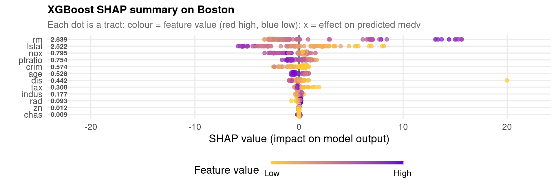
SHAP values (Lundberg & Lee 2017) decompose each individual prediction additively into feature contributions:

\[\hat f(\mathbf{x}_i) = \phi_0 + \sum_{j=1}^{p}\phi_{ij},\]

where \(\phi_{ij}\) is feature \(j\)’s contribution to observation \(i\)’s prediction — the closest thing XGBoost has to a “coefficient”, but local and additive by construction.

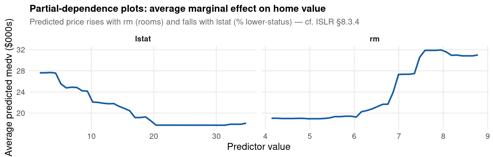
Partial-dependence plots (PDP) show the average marginal effect of one feature, integrating over the others — the non-parametric analogue of a coefficient plot.

PDP, as a formula, is an averaging operation — fix feature \(j\) at a grid value, average the predictions over all rows, repeat:

\[\text{PDP}_j(v) = \frac{1}{n}\sum_{i=1}^{n}\hat f\big(\dots, x_{ij}=v, \dots\big) \quad\Longleftrightarrow\quad \texttt{mean(predict(model, X\_with\_col\_j\_set\_to\_v))}.\]

XGBoost — SHAP and Partial Dependence on Boston

The plot code implements the PDP formula directly: a loop over a grid, setting one column to each grid value and averaging the predictions (no map_ helpers — a plain loop, so the operation is transparent).

SHAP summary (R) — reuses fit_xgb, Xtr
shap_long <- shap.prep(xgb_model = fit_xgb, X_train = Xtr)   # reuse fit from earlier slide
shap.plot.summary(shap_long, dilute = 2) +
  labs(title = "XGBoost SHAP summary on Boston",
       subtitle = "Each dot is a tract; colour = feature value (red high, blue low); x = effect on predicted medv") +
  theme_lecture
Partial dependence for rm and lstat (R)
# Implements PDP_j(v) = mean over rows of f(x with column j set to v)
pdp_curve <- function(model, X, var, grid_n = 40) {
  vals <- seq(min(X[, var]), max(X[, var]), length.out = grid_n)
  yhat <- numeric(grid_n); Xtmp <- X
  for (k in seq_along(vals)) {
    Xtmp[, var] <- vals[k]                                # set column j to v
    yhat[k] <- mean(predict(model, xgb.DMatrix(Xtmp)))    # average prediction
  }
  tibble(value = vals, yhat = yhat, variable = var)
}
bind_rows(pdp_curve(fit_xgb, Xtr, "rm"), pdp_curve(fit_xgb, Xtr, "lstat")) %>%
  ggplot() +
    aes(value, yhat) +
  geom_line(colour = col_main, linewidth = 1.1) +
  facet_wrap(~ variable, scales = "free_x") +
  labs(x = "Predictor value", y = "Average predicted medv ($000s)",
       title = "Partial-dependence plots: average marginal effect on home value",
       subtitle = "Predicted price rises with rm (rooms) and falls with lstat (% lower-status) — cf. ISLR §8.3.4") +
  theme_lecture
SHAP + partial dependence (Python) — reuses model, Xtr, Xte, feat
import numpy as np, matplotlib.pyplot as plt, shap

explainer = shap.TreeExplainer(model)        # reuse fitted model from earlier slide
sv        = explainer(Xte)
mean_abs  = np.abs(sv.values).mean(axis=0)
order     = np.argsort(mean_abs)[::-1]

def pdp_curve(mdl, Xbg, j, grid_n=40):                    # PDP_j(v): set col j to v, average
    grid = np.linspace(Xbg[:, j].min(), Xbg[:, j].max(), grid_n)
    out  = np.empty(grid_n); Xtmp = Xbg.copy()
    for k, v in enumerate(grid):
        Xtmp[:, j] = v
        out[k] = mdl.predict(Xtmp).mean()
    return grid, out

fig, axes = plt.subplots(1, 2, figsize=(11, 3.4))
_ = axes[0].barh([feat[i] for i in order[::-1]], mean_abs[order[::-1]],
                 color="#1a6ea8", alpha=0.85)
_ = axes[0].set_xlabel("Mean |SHAP value|")
_ = axes[0].set_title("Feature importance by SHAP", fontsize=10.5, fontweight="bold")
axes[0].grid(True, axis="x", color="#e8e8e8")
for name, col in [("rm", "#1a6ea8"), ("lstat", "#e8521a")]:
    g, yh = pdp_curve(model, Xtr, feat.index(name))
    _ = axes[1].plot(g, yh, lw=1.6, color=col, label=name)
_ = axes[1].set_xlabel("Predictor value"); _ = axes[1].set_ylabel("Avg predicted medv")
_ = axes[1].set_title("Partial dependence: rm up, lstat down", fontsize=10.5, fontweight="bold")
_ = axes[1].legend(fontsize=9); axes[1].grid(True, color="#e8e8e8")
plt.tight_layout(); plt.show()
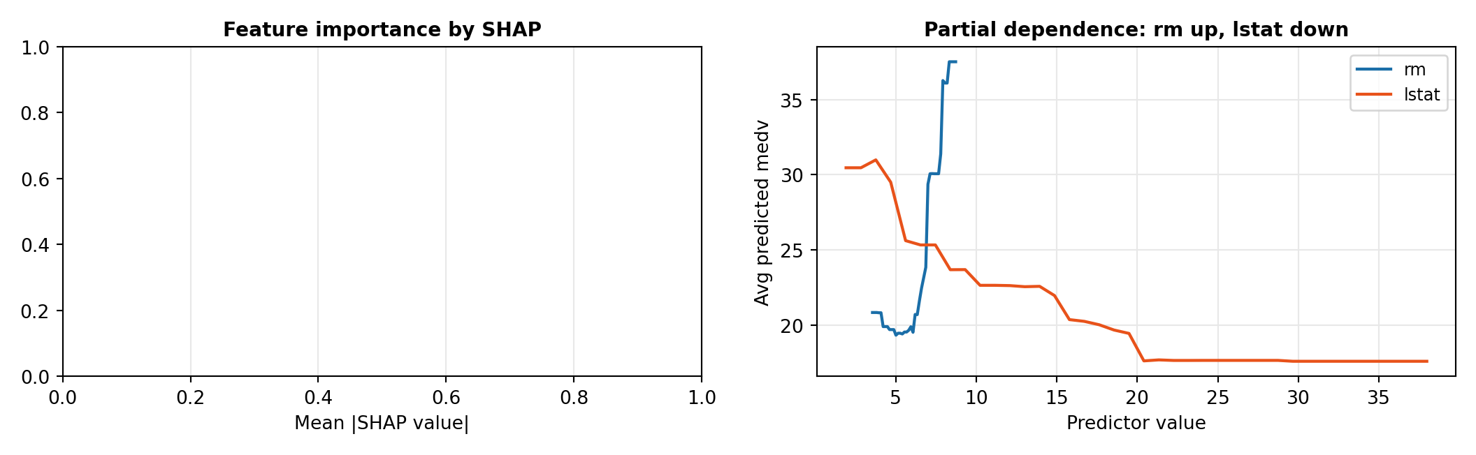
Critical reading. SHAP and PDP describe how the model predicts, not how the world works. A PDP that slopes up for rm says the fitted function increases in rooms holding other features at their observed values — not a causal “effect of adding a room.” For causal questions we need the econometrics of Part V.

Beyond the Average — Individual Conditional Expectation (ICE)

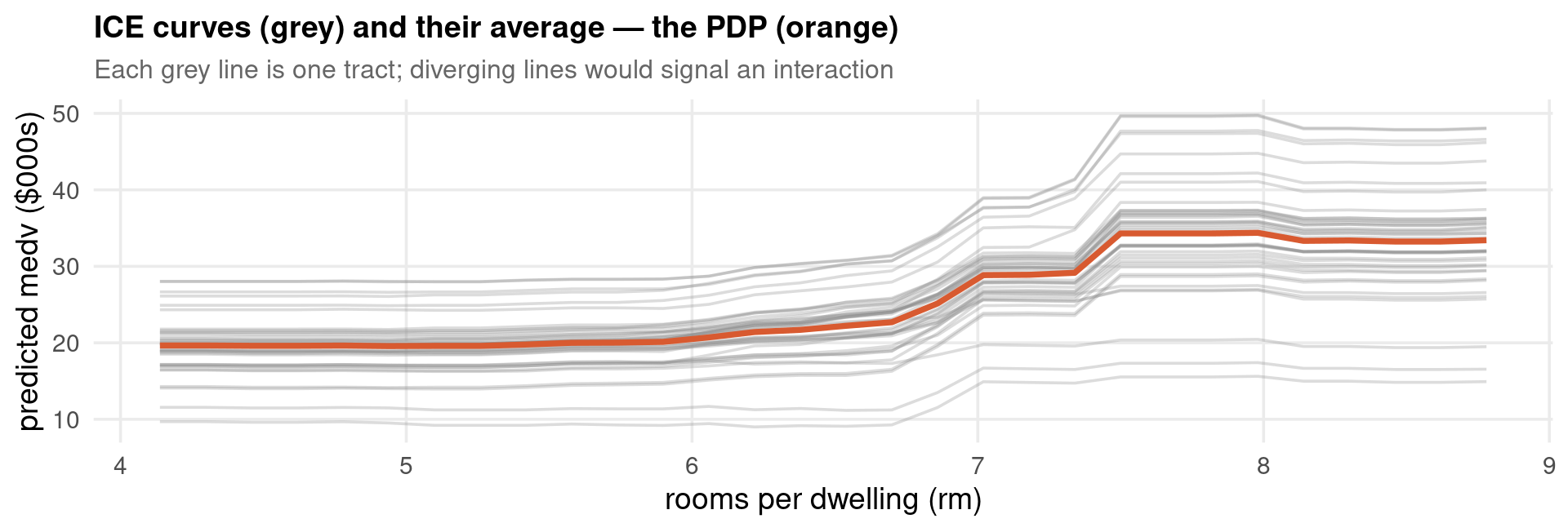
A PDP shows the average marginal effect — but averaging can hide heterogeneity. If rm matters steeply for some tracts and barely for others, the PDP shows only the mean and looks deceptively smooth. ICE curves (Goldstein et al. 2015) disaggregate the PDP into one curve per observation:

\[\text{ICE}_i(v) = \hat f\big(x_{i1},\dots,x_{ij}=v,\dots,x_{ip}\big), \qquad \text{PDP}_j(v) = \frac{1}{n}\sum_{i=1}^{n}\text{ICE}_i(v).\]

The PDP is literally the average of the ICE curves. When the ICE curves are parallel, the effect is homogeneous and the PDP tells the whole story; when they fan out or cross, the feature interacts with the others — the same heterogeneity that motivates causal forests in Part V.

ICE + PDP for rooms (R) — reuses fit_xgb, Xtr
set.seed(SEED)
# ICE: vary one feature over a grid for a sample of rows, keep EACH row's curve
ice_curves <- function(model, X, var, n_ice = 40, grid_n = 30) {
  rows  <- sample(nrow(X), min(n_ice, nrow(X)))
  vals  <- seq(min(X[, var]), max(X[, var]), length.out = grid_n)
  Xsub  <- X[rows, , drop = FALSE]
  parts <- vector("list", length(vals))            # explicit loop, no map_
  for (k in seq_along(vals)) {
    Xtmp <- Xsub; Xtmp[, var] <- vals[k]
    parts[[k]] <- tibble(id = rows, value = vals[k],
                         yhat = predict(model, xgb.DMatrix(Xtmp)))
  }
  bind_rows(parts)
}
ice_df <- ice_curves(fit_xgb, Xtr, "rm")
pdp_df <- ice_df %>% summarise(yhat = mean(yhat), .by = value)   # PDP = mean of ICE
ggplot(ice_df) +
  aes(value, yhat, group = id) +
  geom_line(colour = col_muted, alpha = 0.30) +
  geom_line(data = pdp_df, aes(value, yhat), inherit.aes = FALSE,
            colour = col_accent, linewidth = 1.3) +
  labs(x = "rooms per dwelling (rm)", y = "predicted medv ($000s)",
       title = "ICE curves (grey) and their average — the PDP (orange)",
       subtitle = "Each grey line is one tract; diverging lines would signal an interaction") +
  theme_lecture
ICE + PDP for rooms (Python) — reuses model, Xtr, feat
import matplotlib.pyplot as plt
from sklearn.inspection import PartialDependenceDisplay
fig, ax = plt.subplots(figsize=(7.5, 3.4))
# kind="both" overlays the individual ICE curves and their average (the PDP)
_ = PartialDependenceDisplay.from_estimator(
        model, Xtr, [feat.index("rm")], kind="both",
        subsample=40, random_state=SEED, ax=ax)
_ = ax.set_title("ICE curves and their average (PDP) for rooms (rm)",
                 fontsize=10.5, fontweight="bold")
plt.tight_layout(); plt.show()
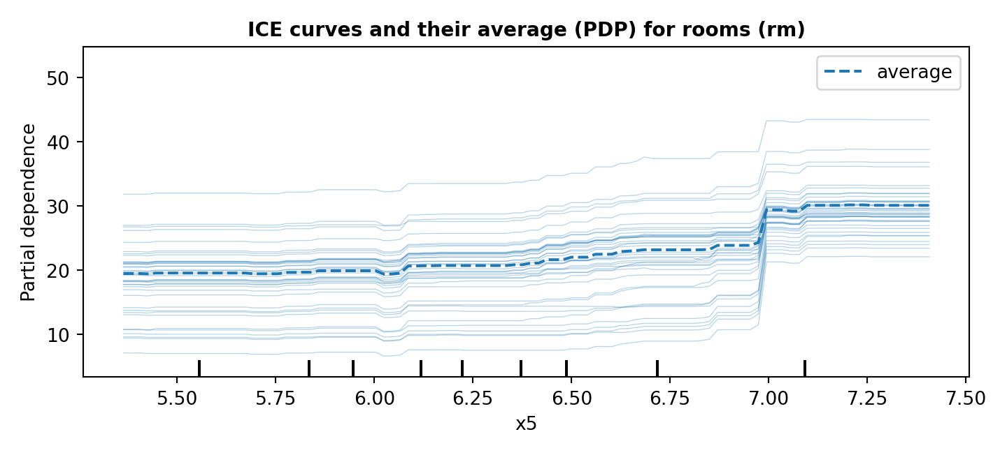
Reading note: parallel ICE curves ⇒ a homogeneous effect; curves that fan out or cross ⇒ an interaction the PDP conceals. ICE is the bridge from average description to the heterogeneous causal effects of Part V.

Part V — Trees for Econometrics

“Great predictions — but where is the coefficient?”

A Prediction Shoot-out — Setup

Before the econometrics, one honest question: on real data, do trees actually beat the linear methods you already use? We race five methods on the Boston test set: OLS, Lasso, Ridge, a random forest, and XGBoost.

  • Data / split: the same 50/50 Boston split as before.
  • Metric: out-of-sample RMSE (lower is better), plus the % change versus OLS.
  • Fair comparison: every method sees the same training rows and is scored on the same held-out rows.

The next slide runs all five and sorts them. Watch whether the non-linear methods (forest, XGBoost) win — if they do, the conditional mean really is non-linear with interactions.

A Prediction Shoot-out — Estimate and Read

Five methods, one held-out test set (R)
set.seed(SEED)
xvars <- setdiff(names(boston), "medv")
n     <- nrow(boston); train <- sample(n, floor(n / 2))
Xtr   <- as.matrix(boston[train,  xvars]); ytr <- boston$medv[train]
Xte   <- as.matrix(boston[-train, xvars]); yte <- boston$medv[-train]
rmse  <- function(a, b) sqrt(mean((a - b)^2))

fit_ols   <- lm(medv ~ ., data = boston[train, ])
fit_lasso <- cv.glmnet(Xtr, ytr, alpha = 1, nfolds = N_CV_FOLDS)   # alpha=1 -> Lasso
fit_ridge <- cv.glmnet(Xtr, ytr, alpha = 0, nfolds = N_CV_FOLDS)   # alpha=0 -> Ridge
fit_forest<- ranger(medv ~ ., data = boston[train, ], num.trees = N_TREES,
                    mtry = floor(length(xvars) / 3), num.threads = N_THREADS, seed = SEED)
fit_boost <- xgb.train(list(objective = "reg:squarederror", max_depth = 3, eta = 0.05,
                            subsample = 0.8, colsample_bytree = 0.8, lambda = 1),
                       xgb.DMatrix(Xtr, label = ytr), nrounds = 1000,
                       evals = list(train = xgb.DMatrix(Xtr, label = ytr),
                                        test  = xgb.DMatrix(Xte, label = yte)),
                       early_stopping_rounds = 30, verbose = 0)

tibble(Method = c("OLS", "Lasso", "Ridge", "Random forest", "XGBoost"),
       `Test RMSE` = c(rmse(yte, predict(fit_ols, boston[-train, ])),
                       rmse(yte, as.numeric(predict(fit_lasso, Xte, s = "lambda.min"))),
                       rmse(yte, as.numeric(predict(fit_ridge, Xte, s = "lambda.min"))),
                       rmse(yte, predict(fit_forest, boston[-train, ])$predictions),
                       rmse(yte, predict(fit_boost,  xgb.DMatrix(Xte))))) %>%
  arrange(`Test RMSE`) %>%
  mutate(`vs OLS` = sprintf("%+.1f%%", 100 * (`Test RMSE` / `Test RMSE`[Method == "OLS"] - 1))) %>%
  kbl(caption = "Boston: out-of-sample RMSE, 50/50 split (lower is better)", digits = 3) %>%
  kable_styling(font_size = 20, full_width = TRUE) %>%
  row_spec(1, bold = TRUE, color = "white", background = col_main)
Boston: out-of-sample RMSE, 50/50 split (lower is better)
Method Test RMSE vs OLS
XGBoost 3.889 -26.8%
Random forest 4.009 -24.6%
OLS 5.314 +0.0%
Lasso 5.348 +0.7%
Ridge 5.439 +2.4%
Five methods, one held-out test set (Python)
import pandas as pd, numpy as np
from sklearn.linear_model import LinearRegression, LassoCV, RidgeCV
from sklearn.ensemble import RandomForestRegressor
from sklearn.model_selection import train_test_split
from sklearn.metrics import mean_squared_error
import xgboost as xgb

boston = pd.read_csv("../data/boston.csv")
feat = [c for c in boston.columns if c != "medv"]
X = boston[feat].to_numpy(dtype=float); y = boston["medv"].to_numpy(dtype=float)
Xtr, Xte, ytr, yte = train_test_split(X, y, test_size=0.5, random_state=SEED)
rmse = lambda a, b: mean_squared_error(a, b) ** 0.5

ols = LinearRegression().fit(Xtr, ytr)
las = LassoCV(cv=N_CV_FOLDS, max_iter=10000, random_state=SEED).fit(Xtr, ytr)
rid = RidgeCV(alphas=np.logspace(-3, 3, 50)).fit(Xtr, ytr)
rf  = RandomForestRegressor(n_estimators=N_TREES, max_features=max(1, X.shape[1] // 3),
                            n_jobs=N_CORES, random_state=SEED).fit(Xtr, ytr)
xgm = xgb.XGBRegressor(objective="reg:squarederror", max_depth=3, learning_rate=0.05,
                       subsample=0.8, colsample_bytree=0.8, reg_lambda=1.0,
                       n_estimators=1000, early_stopping_rounds=30, eval_metric="rmse",
                       random_state=SEED, n_jobs=N_CORES)
xgm.fit(Xtr, ytr, eval_set=[(Xte, yte)], verbose=False)

rows = [("OLS", rmse(yte, ols.predict(Xte))), ("Lasso", rmse(yte, las.predict(Xte))),
        ("Ridge", rmse(yte, rid.predict(Xte))), ("Random forest", rmse(yte, rf.predict(Xte))),
        ("XGBoost", rmse(yte, xgm.predict(Xte)))]
rows.sort(key=lambda r: r[1])
from tabulate import tabulate
print(tabulate([(m, f"{r:.3f}") for m, r in rows],
               headers=["Method", "Test RMSE"], tablefmt="rounded_outline"))
Five methods, one held-out test set (Stata, pystacked)
* pystacked fits all base learners in one call; gradboost is scikit-learn's gradient
* boosting (close cousin of XGBoost). Needs: ssc install pystacked
import delimited "../data/boston.csv", clear
set seed 14159
generate byte train = runiform() < 0.5
pystacked medv crim zn indus chas nox rm age dis rad tax ptratio lstat ///
    if train, type(reg) methods(ols lassocv ridgecv rf gradboost) pyseed(14159)
* `transform` returns one prediction column per base learner, in the order listed
predict double yh, transform
local names OLS Lasso Ridge RF GradBoost
local k = 1
foreach nm of local names {
    quietly generate double se`k' = (medv - yh`k')^2 if !train
    quietly summarize se`k' if !train
    display as text "`nm' test RMSE: " as result %6.3f sqrt(r(mean))
    local ++k
}
> radient
(encoding automatically selected: ISO-8859-1)
(13 vars, 506 obs)


Error loading Python Script for pystacked.
unrecognized command
r(199);

r(199);

What this shows — and what it does not. On Boston the tree ensembles typically win on pure prediction: the conditional mean is non-linear with interactions, so flexibility pays. But a low RMSE is not an economic finding. None of these is a coefficient with a standard error. To answer “what is the union wage premium?” we must convert prediction power into valid inference.

From Prediction to Inference — FWL, the Linear Case

You already know how to isolate one coefficient from many controls: the Frisch–Waugh–Lovell (FWL) theorem. To get \(\beta\) in \(y = D\beta + \mathbf{X}\boldsymbol\gamma + \varepsilon\) you may

  1. regress \(y\) on \(\mathbf{X}\), keep residuals \(\tilde y\);
  2. regress \(D\) on \(\mathbf{X}\), keep residuals \(\tilde D\);
  3. regress \(\tilde y\) on \(\tilde D\) — the slope is exactly \(\hat\beta\).

FWL, in code — three regressions, and the third gives the coefficient:

FWL on Boston: residual slope = direct coefficient (R)
ctrl <- "rm + age + dis + tax + ptratio"          # controls X; treat lstat as D
yres <- residuals(lm(as.formula(paste("medv  ~", ctrl)), data = boston))
Dres <- residuals(lm(as.formula(paste("lstat ~", ctrl)), data = boston))
beta_fwl    <- coef(lm(yres ~ Dres))[[2]]
beta_direct <- coef(lm(as.formula(paste("medv ~ lstat +", ctrl)), data = boston))[["lstat"]]
c(FWL_residual_slope = beta_fwl, direct_coefficient = beta_direct)   # identical
FWL_residual_slope direct_coefficient 
        -0.5951328         -0.5951328 
FWL on Boston (Python)
import pandas as pd, statsmodels.api as sm, statsmodels.formula.api as smf
boston = pd.read_csv("../data/boston.csv")
ctrl = "rm + age + dis + tax + ptratio"
yres = smf.ols(f"medv  ~ {ctrl}", boston).fit().resid
Dres = smf.ols(f"lstat ~ {ctrl}", boston).fit().resid
beta_fwl    = sm.OLS(yres, sm.add_constant(Dres)).fit().params.iloc[1]
beta_direct = smf.ols(f"medv ~ lstat + {ctrl}", boston).fit().params["lstat"]
print(f"FWL residual slope: {beta_fwl:.4f}   direct coefficient: {beta_direct:.4f}")
FWL on Boston: residual slope = direct coefficient (Stata)
import delimited "../data/boston.csv", clear
quietly regress medv  rm age dis tax ptratio
predict y_res, residuals
quietly regress lstat rm age dis tax ptratio
predict d_res, residuals
regress y_res d_res                       // slope on d_res = FWL beta
regress medv lstat rm age dis tax ptratio // compare: coefficient on lstat matches
(encoding automatically selected: ISO-8859-1)
(13 vars, 506 obs)

      Source |       SS           df       MS      Number of obs   =       506
-------------+----------------------------------   F(1, 504)       =    131.56
       Model |   3376.2126         1   3376.2126   Prob > F        =    0.0000
    Residual |  12934.5032       504  25.6636969   R-squared       =    0.2070
-------------+----------------------------------   Adj R-squared   =    0.2054
       Total |  16310.7158       505  32.2984472   Root MSE        =    5.0659

------------------------------------------------------------------------------
       y_res | Coefficient  Std. err.      t    P>|t|     [95% conf. interval]
-------------+----------------------------------------------------------------
       d_res |  -.5951328    .051887   -11.47   0.000    -.6970743   -.4931914
       _cons |  -1.05e-08   .2252083    -0.00   1.000    -.4424627    .4424626
------------------------------------------------------------------------------

      Source |       SS           df       MS      Number of obs   =       506
-------------+----------------------------------   F(6, 499)       =    191.49
       Model |  29781.7923         6  4963.63205   Prob > F        =    0.0000
    Residual |  12934.5033       499  25.9208483   R-squared       =    0.6972
-------------+----------------------------------   Adj R-squared   =    0.6936
       Total |  42716.2956       505   84.586724   Root MSE        =    5.0913

------------------------------------------------------------------------------
        medv | Coefficient  Std. err.      t    P>|t|     [95% conf. interval]
-------------+----------------------------------------------------------------
       lstat |  -.5951328   .0521463   -11.41   0.000    -.6975862   -.4926794
          rm |   4.415709   .4260045    10.37   0.000     3.578725    5.252692
         age |  -.0193475   .0133963    -1.44   0.149    -.0456675    .0069726
         dis |  -.8430649   .1686935    -5.00   0.000    -1.174502   -.5116279
         tax |  -.0054857   .0018295    -3.00   0.003    -.0090802   -.0018912
     ptratio |  -.8414776   .1223353    -6.88   0.000    -1.081833   -.6011219
       _cons |   24.60754   4.086002     6.02   0.000     16.57966    32.63543
------------------------------------------------------------------------------

This “partials out” \(\mathbf{X}\)linearly. The next slide asks what happens when the controls do not enter linearly.

From Prediction to Inference — Robinson’s Partially Linear Model

What if the controls do not enter linearly? Robinson (1988) gives the answer with the partially linear model

\[y = D\,\beta + g(\mathbf{X}) + \varepsilon,\qquad \mathbb{E}[\varepsilon\mid D,\mathbf{X}]=0,\]

where \(g(\cdot)\) is an unknown, possibly highly non-linear function. The same three steps work — but the partialling-out now uses non-parametric predictions:

\[\tilde y_i = y_i - \hat{\mathbb{E}}[y\mid\mathbf{X}_i],\qquad \tilde D_i = D_i - \hat{\mathbb{E}}[D\mid\mathbf{X}_i],\qquad \hat\beta = \frac{\sum_i \tilde D_i\,\tilde y_i}{\sum_i \tilde D_i^2}.\]

The only change from the previous slide is how we predict \(\mathbb{E}[y\mid\mathbf{X}]\) and \(\mathbb{E}[D\mid\mathbf{X}]\) — swap lm() for a forest:

y_res <- y - ranger(y ~ X, data = df)$predictions   # OOB predictions = E[y|X], non-parametric
D_res <- D - ranger(D ~ X, data = df)$predictions    # OOB predictions = E[D|X]
beta  <- coef(lm(y_res ~ D_res))[2]                   # same FWL slope, flexible nuisance
y_res = y - RandomForestRegressor(oob_score=True).fit(X, y).oob_prediction_   # E[y|X]
D_res = D - RandomForestRegressor(oob_score=True).fit(X, D).oob_prediction_   # E[D|X]
beta  = sm.OLS(y_res, sm.add_constant(D_res)).fit().params[1]                 # FWL slope
* ddml does the forest partialling-out and the FWL step together:
ddml init partial, kfolds(5)
ddml E[Y|X]: pystacked y x*, type(reg) methods(rf)
ddml E[D|X]: pystacked d x*, type(reg) methods(rf)
ddml crossfit
ddml estimate, robust         // beta on the residualised treatment

This is the whole point of the lecture. A random forest or XGBoost is simply a flexible estimator of the two conditional expectations. Plug them into FWL and you recover a single, interpretable \(\hat\beta\) with a standard error — even though the controls were handled by a black box.

From Prediction to Inference — Why Out-of-Sample Predictions?

One subtlety separates a valid estimate from a biased one.

If the same observation is used both to fit the nuisance and to form its residual, the flexible learner partly fits the noise in that point — its overfitting bias leaks into \(\hat\beta\) and pulls it toward zero. The cure is to predict each \(\mathbf{X}_i\) with a model that did not see observation \(i\):

  • Random forest: use the out-of-bag prediction — free, and effectively leave-one-out.
  • XGBoost: use K-fold cross-fitting — predict each fold from a model trained on the others.

Cross-fitting, in code — loop over folds, train on the rest, predict the held-out fold:

pred <- numeric(length(y))
for (k in unique(folds)) {
  m            <- xgb.train(params, xgb.DMatrix(X[folds != k, ], label = y[folds != k]), nrounds = 300)
  pred[folds == k] <- predict(m, xgb.DMatrix(X[folds == k, ]))   # predict the unseen fold
}
from sklearn.model_selection import KFold
pred = np.zeros(len(y))
for tr, te in KFold(5, shuffle=True, random_state=SEED).split(X):
    m = xgb.XGBRegressor(n_estimators=300).fit(X[tr], y[tr])
    pred[te] = m.predict(X[te])                                  # predict the unseen fold
ddml crossfit        // K-fold out-of-fold nuisance predictions, generated automatically

This is exactly the cross-fitting step of Double/Debiased ML (Chernozhukov et al. 2018), developed in full in the companion deck. Here we take its first step with tree nuisance.

Application: The Union Premium — Step 1–2, Data and Prep

We now answer the running question: does replacing TWFE’s linear controls with a forest or XGBoost move the union wage premium?

  • Data: wagepan — 545 young men, 1980–1987 (a balanced panel). Outcome lwage, treatment union, plus demographics and industry/occupation dummies.
  • Prepare (two steps): (1) within-demean every variable by individual (nr) to remove the person fixed effect — the panel analogue of FWL’s first partialling; (2) build clean year dummies for the time effect. The demeaned outcome/treatment and the controls then feed the tree partial-out.
# Within-individual demeaning = remove the nr fixed effect (tidyverse style)
wp_dm <- wp %>%
  group_by(nr) %>%
  mutate(across(c(lwage, union, all_of(ctrl_vars)),
                ~ . - mean(.))) %>%   # subtract each person's own mean
  ungroup()

The benchmark is the linear TWFE union premium, \(\hat\beta^{\text{union}}\approx 0.08\). The question is whether a flexible nuisance moves it.

Application: The Union Premium — Step 3, Estimate

We estimate three ways: linear TWFE (benchmark), RF partial-out using OOB residuals, and XGBoost partial-out using K-fold cross-fitting.

RF (OOB) and XGBoost (cross-fit) partial-out (R)
.wpt    <- wp_prep()                       # prepared in the setup: demeaned y, D, controls + TWFE
ctrl_w  <- .wpt$ctrl;  y_w <- .wpt$y;  D_w <- .wpt$D
b_twfe  <- .wpt$twfe$b; se_twfe <- .wpt$twfe$se

# One frame per nuisance regression (controls only on the RHS); using `y ~ .` on a
# frame that excludes the other target avoids ranger's fragile `. - var` handling.
df_y <- data.frame(y = y_w, ctrl_w, check.names = TRUE)
df_d <- data.frame(D = D_w, ctrl_w, check.names = TRUE)

set.seed(SEED)
rf_y <- ranger(y ~ ., data = df_y, num.trees = N_TREES, min.node.size = 5,
               num.threads = N_THREADS, seed = SEED)   # $predictions are OOB (free cross-fit)
rf_d <- ranger(D ~ ., data = df_d, num.trees = N_TREES, min.node.size = 5,
               num.threads = N_THREADS, seed = SEED)
ols_rf <- lm((y_w - rf_y$predictions) ~ I(D_w - rf_d$predictions))   # FWL on residuals
b_rf   <- coef(ols_rf)[[2]]
se_rf  <- sqrt(sandwich::vcovHC(ols_rf, type = "HC3")[2, 2])         # robust SE

# XGBoost nuisance — honest K-fold cross-fitting (out-of-fold predictions)
Xw   <- as.matrix(ctrl_w)
xpar <- list(objective = "reg:squarederror", max_depth = 4, eta = 0.05,
             subsample = 0.8, colsample_bytree = 0.8, lambda = 1)
crossfit_xgb <- function(X, target, folds) {
  pred <- numeric(length(target))
  for (k in sort(unique(folds))) {
    in_tr <- folds != k
    m <- xgb.train(xpar, xgb.DMatrix(X[in_tr, , drop = FALSE], label = target[in_tr]),
                   nrounds = 300, verbose = 0)
    pred[!in_tr] <- predict(m, xgb.DMatrix(X[!in_tr, , drop = FALSE]))
  }
  pred
}
set.seed(SEED)
folds  <- sample(rep_len(seq_len(N_CV_FOLDS), length(y_w)))
ols_xg <- lm((y_w - crossfit_xgb(Xw, y_w, folds)) ~ I(D_w - crossfit_xgb(Xw, D_w, folds)))
b_xgb  <- coef(ols_xg)[[2]]
se_xgb <- sqrt(sandwich::vcovHC(ols_xg, type = "HC3")[2, 2])

tibble(Estimator = c("TWFE (linear, hand-picked)", "RF partial-out (OOB)",
                     "XGBoost partial-out (cross-fit)"),
       `Union premium` = c(b_twfe, b_rf, b_xgb),
       SE = c(se_twfe, se_rf, se_xgb),
       Nuisance = c("Linear FE", "Random forest", "XGBoost")) %>%
  mutate(`95% CI` = sprintf("[%.3f, %.3f]", `Union premium` - 1.96 * SE,
                            `Union premium` + 1.96 * SE)) %>%
  kbl(caption = "wagepan: union wage premium — linear vs tree-based nuisance", digits = 4) %>%
  kable_styling(font_size = 19, full_width = TRUE) %>%
  row_spec(2:3, bold = TRUE, color = "white", background = col_main)
wagepan: union wage premium — linear vs tree-based nuisance
Estimator Union premium SE Nuisance 95% CI
TWFE (linear, hand-picked) 0.0800 0.0227 Linear FE [0.036, 0.124]
RF partial-out (OOB) 0.0831 0.0180 Random forest [0.048, 0.118]
XGBoost partial-out (cross-fit) 0.0872 0.0184 XGBoost [0.051, 0.123]
RF (OOB) and XGBoost (cross-fit) partial-out (Python)
import pandas as pd, numpy as np, warnings
warnings.filterwarnings("ignore")
from sklearn.ensemble import RandomForestRegressor
from sklearn.model_selection import KFold
import xgboost as xgb

try:
    import wooldridge as woo; wp = woo.data("wagepan")
except Exception:
    wp = pd.read_csv("../data/wagepan.csv")

base = [c for c in ["exper","expersq","married","educ","black","hisp","south","smsa"] if c in wp.columns]
ind  = [c for c in ["agric","bus","construc","ndurman","trcommpu","trade",
                    "services","profserv","profocc","clerocc","servocc"] if c in wp.columns]
ctrl = base + ind
wp   = wp[["nr","year","lwage","union"] + ctrl].dropna()

num = ["lwage","union"] + ctrl                                   # within-demean by nr
wp_dm = wp.copy()
wp_dm[num] = wp_dm[num] - wp_dm.groupby("nr")[num].transform("mean")
yr = pd.get_dummies(wp_dm["year"], prefix="yr", drop_first=True).astype(float)
X = np.column_stack([wp_dm[ctrl].to_numpy(dtype=float), yr.to_numpy(dtype=float)])
y = wp_dm["lwage"].to_numpy(dtype=float); D = wp_dm["union"].to_numpy(dtype=float)

b_twfe = np.linalg.lstsq(np.column_stack([D, X]), y, rcond=None)[0][0]

def partial_out(yres, Dres):                                     # FWL slope + HC0 robust SE
    b = (Dres @ yres) / (Dres @ Dres)
    resid = yres - b * Dres
    se = np.sqrt(np.sum(Dres**2 * resid**2)) / (Dres @ Dres)
    return b, se

rf_y = RandomForestRegressor(n_estimators=N_TREES, min_samples_leaf=5, oob_score=True,
                             bootstrap=True, n_jobs=N_CORES, random_state=SEED).fit(X, y)
rf_d = RandomForestRegressor(n_estimators=N_TREES, min_samples_leaf=5, oob_score=True,
                             bootstrap=True, n_jobs=N_CORES, random_state=SEED).fit(X, D)
b_rf, se_rf = partial_out(y - rf_y.oob_prediction_, D - rf_d.oob_prediction_)

def crossfit_xgb(X, target):
    pred = np.zeros_like(target, dtype=float)
    for tr, te in KFold(n_splits=N_CV_FOLDS, shuffle=True, random_state=SEED).split(X):
        m = xgb.XGBRegressor(objective="reg:squarederror", max_depth=4, learning_rate=0.05,
                             subsample=0.8, colsample_bytree=0.8, reg_lambda=1.0,
                             n_estimators=300, random_state=SEED, n_jobs=N_CORES)
        m.fit(X[tr], target[tr]); pred[te] = m.predict(X[te])
    return pred
b_xgb, se_xgb = partial_out(y - crossfit_xgb(X, y), D - crossfit_xgb(X, D))

from tabulate import tabulate
print(tabulate([["TWFE (linear)", f"{b_twfe:.4f}", "—"],
                ["RF partial-out (OOB)", f"{b_rf:.4f}", f"{se_rf:.4f}"],
                ["XGBoost partial-out (cross-fit)", f"{b_xgb:.4f}", f"{se_xgb:.4f}"]],
               headers=["Estimator", "Union premium", "Robust SE"], tablefmt="rounded_outline"))
TWFE + DML partial-out (ddml + pystacked, Stata)
frause wagepan, clear
xtset nr year

* TWFE benchmark (same specification as the companion deck)
xtreg lwage union exper expersq married educ i.year, fe vce(cluster nr)
display as text "TWFE union premium: " as result %7.4f _b[union]

* To match the R/Python tabs, FIRST remove the nr fixed effect by within-demeaning,
* THEN partial out the demeaned controls + year dummies with a forest.
* One-time: ssc install ddml ; ssc install pystacked
local ctrls exper expersq married educ black hisp south smsa
foreach v of varlist lwage union `ctrls' {
    bysort nr (year): egen double m_`v' = mean(`v')
    generate double dm_`v' = `v' - m_`v'
}
local dmctrls
foreach v of local ctrls {
    local dmctrls `dmctrls' dm_`v'
}
ddml init partial, kfolds(5)
ddml E[Y|X]: pystacked dm_lwage `dmctrls' i.year, type(reg) methods(rf) pyseed(14159)
ddml E[D|X]: pystacked dm_union `dmctrls' i.year, type(reg) methods(rf) pyseed(14159)
ddml crossfit
ddml estimate, robust
Panel variable: nr (strongly balanced)
 Time variable: year, 1980 to 1987
         Delta: 1 unit

note: educ omitted because of collinearity.
note: 1987.year omitted because of collinearity.

Fixed-effects (within) regression               Number of obs     =      4,360
Group variable: nr                              Number of groups  =        545

R-squared:                                      Obs per group:
     Within  = 0.1806                                         min =          8
     Between = 0.0005                                         avg =        8.0
     Overall = 0.0635                                         max =          8

                                                F(10, 544)        =      46.59
corr(u_i, Xb) = -0.1212                         Prob > F          =     0.0000

                                   (Std. err. adjusted for 545 clusters in nr)
------------------------------------------------------------------------------
             |               Robust
       lwage | Coefficient  std. err.      t    P>|t|     [95% conf. interval]
-------------+----------------------------------------------------------------
       union |   .0800019   .0227431     3.52   0.000     .0353268    .1246769
       exper |   .1321464    .012008    11.00   0.000     .1085586    .1557342
     expersq |  -.0051855   .0008102    -6.40   0.000    -.0067771   -.0035939
     married |   .0466804   .0210038     2.22   0.027     .0054218    .0879389
        educ |          0  (omitted)
             |
        year |
       1981  |   .0190448   .0227267     0.84   0.402     -.025598    .0636876
       1982  |   -.011322   .0212167    -0.53   0.594    -.0529987    .0303547
       1983  |  -.0419955   .0205087    -2.05   0.041    -.0822814   -.0017096
       1984  |  -.0384709   .0211722    -1.82   0.070    -.0800601    .0031183
       1985  |  -.0432498    .017595    -2.46   0.014    -.0778122   -.0086874
       1986  |  -.0273819   .0162181    -1.69   0.092    -.0592396    .0044757
       1987  |          0  (omitted)
             |
       _cons |    1.02764   .0398919    25.76   0.000     .9492785    1.106001
-------------+----------------------------------------------------------------
     sigma_u |   .4009279
     sigma_e |  .35099001
         rho |  .56612236   (fraction of variance due to u_i)
------------------------------------------------------------------------------

TWFE union premium:  0.0800


variable smsa not found
r(111);

r(111);

Parameters worth noting. min.node.size/min_samples_leaf = 5 regularises each tree; kfolds(5) / N_CV_FOLDS sets the cross-fitting folds; vcovHC(., "HC3") and the HC0 formula give heteroskedasticity-robust SEs on the final FWL regression.

Application: The Union Premium — Step 4, Read the Table

How should you read this table? Compare the tree-based premia to the TWFE benchmark of \(\approx 0.08\):

  • If RF/XGBoost partial-out land close to TWFE, the linear, hand-picked control set was already adequate — the non-linearities are modest, and the simpler estimator is preferable for transparency.
  • If they diverge, non-linear confounding matters: the flexible nuisance is correcting bias the linear specification could not. That is the case for using trees.

Either way, the honest comparison required OOB / cross-fitted nuisance — in-sample tree fits would have biased \(\hat\beta\) toward zero through overfitting (you verify this in Exercise 5).

The discipline to report: the estimand (\(\hat\beta^{\text{union}}\)), the nuisance learner, the cross-fitting scheme, the robust SE, and the seed. A reader should be able to reproduce the number exactly.

Beyond One Number — Causal Forests

The partial-out estimator returns a single average premium. But what if the union effect differs across workers — larger for low-tenure workers, smaller in some industries? Averaging hides that heterogeneity.

Causal forests (Wager & Athey 2018) adapt the random forest to estimate the conditional average treatment effect

\[\tau(\mathbf{x}) = \mathbb{E}[\,Y(1)-Y(0)\mid \mathbf{X}=\mathbf{x}\,],\]

by growing trees whose splits maximise treatment-effect heterogeneity rather than predictive fit, with honest sample-splitting so each leaf’s estimate is valid. The forest then delivers a personalised \(\hat\tau(\mathbf{x})\) with pointwise confidence intervals.

Goal Estimator Software
One average effect, flexible controls Partial-out / DML R DoubleML, Stata ddml, Py econml
Heterogeneous effect \(\tau(\mathbf{x})\) Causal forest R grf::causal_forest, Py econml.CausalForestDML
# The estimand changes from a scalar beta to a function tau(x):
library(grf)
cf  <- causal_forest(X, Y, W)        # W = treatment, X = covariates
tau <- predict(cf)$predictions       # one estimated effect PER observation
from econml.dml import CausalForestDML
cf  = CausalForestDML().fit(Y, W, X=X)   # W = treatment, X = covariates
tau = cf.effect(X)                       # one estimated effect PER observation
* No native causal forest; estimate the heterogeneous effect through ddml's
* interactive model, or call econml/grf via Stata's Python integration.
ddml init interactive, kfolds(5)

This is the bridge from prediction (Parts II–IV) through one causal number (Part V) to causal heterogeneity. The full treatment — orthogonal moments, cross-fitting, inference on \(\tau(\mathbf{x})\) — is the subject of the companion deck and Chapter 14 of the Causal ML book.

From Effects to Decisions — Policy Learning

Estimating \(\tau(\mathbf{x})\) answers “for whom is the effect large?” The next question is a decision: whom should we treat? This is policy learning (Athey & Wager 2021), the payoff of the Stanford ML-CI tutorial.

The building block is the doubly-robust (AIPW) score — combining the outcome model \(\hat g\) and the propensity \(\hat e(\mathbf{x})=\mathbb{P}(D=1\mid\mathbf{x})\) so the estimate stays valid if either is consistent:

\[\hat\Gamma_i = \hat\tau(\mathbf{x}_i) + \frac{D_i-\hat e(\mathbf{x}_i)}{\hat e(\mathbf{x}_i)\,(1-\hat e(\mathbf{x}_i))}\Big(Y_i - \hat g(\mathbf{x}_i, D_i)\Big).\]

A policy \(\pi:\mathcal{X}\to\{0,1\}\) is then chosen to maximise estimated value \(\frac{1}{n}\sum_i \pi(\mathbf{x}_i)\hat\Gamma_i\). Restricting \(\pi\) to a shallow policy tree yields an interpretable, deployable targeting rule — a few yes/no questions a programme administrator can follow.

library(policytree)
dr  <- double_robust_scores(cf)          # AIPW scores from the causal forest cf
tree <- policy_tree(X, dr, depth = 2)    # shallow, interpretable assignment rule
predict(tree, X)                         # whom to treat: 1 = treat, 0 = do not
from econml.policy import PolicyTree
pol = PolicyTree(max_depth=2).fit(X, dr_scores)   # dr_scores = AIPW scores
pol.predict(X)                                    # 1 = treat, 0 = do not
* No native policy-tree command; build AIPW scores with ddml/teffects, then call
* policytree (R) or econml (Python) through Stata's language bridge.

Why doubly robust? The AIPW score gives valid policy evaluation if either the outcome model or the propensity is right — exactly the robustness Double/Debiased ML buys. References: Athey & Wager (2021); the Stanford ML-CI tutorial, Ch. 5–6.

Part VI — Forecasting Time Series

Where XGBoost wins on tabular data of any kind — including the temporal kind

Why Trees for Time Series?

Trees do not model time. We reframe forecasting as supervised learning: regress \(y_t\) on its own recent past.

\[\hat y_t = f\!\left(y_{t-1},\,y_{t-2},\dots,y_{t-p},\ \text{season}_t,\ \mathbf{x}_t\right).\]

Where XGBoost beats ARIMA:

  • Non-linear dynamics — thresholds, regime shifts, asymmetric responses.
  • Many predictors — dozens of lags plus exogenous series, regularised automatically.
  • No order to specify — no \((p,d,q)\), no stationarity diagnostics by hand.
  • Seasonality — a calendar feature lets one model split on the month.

Under the Hood — What XGBoost Fits

With lag features the model is a non-linear, non-parametric AR(\(p\)):

\[\Delta y_t = f(\Delta y_{t-1},\dots,\Delta y_{t-p},\,\text{month}_t) + \varepsilon_t, \qquad f(\mathbf{x}) = \sum_{m=1}^{M} f_m(\mathbf{x}),\quad f_m \in \text{trees}.\]

Each round \(m\) adds the tree minimising the second-order objective

\[\mathcal{L}^{(m)} = \sum_t \left[ g_t\, f_m(\mathbf{x}_t) + \tfrac12 h_t\, f_m(\mathbf{x}_t)^2 \right] + \gamma T + \tfrac{\lambda}{2}\sum_{j=1}^{T} w_j^2,\]

with \(g_t = \partial_{\hat y} \ell\), \(h_t = \partial^2_{\hat y} \ell\); the optimal leaf value and split gain are

\[w_j^\ast = -\frac{\sum_{t\in R_j} g_t}{\sum_{t\in R_j} h_t + \lambda}, \qquad \text{Gain} = \tfrac12\!\left[\frac{G_L^2}{H_L+\lambda} + \frac{G_R^2}{H_R+\lambda} - \frac{G^2}{H+\lambda}\right] - \gamma.\]

Reading. Replace the linear \(\sum_k \phi_k \Delta y_{t-k}\) of an AR with a sum of step functions: thresholds, interactions, and seasonal asymmetries enter automatically; \(\lambda,\gamma,\eta\) shrink them like Ridge shrinks coefficients.

Two Rules You Cannot Break

  • Train on the past, test on the future. Never shuffle rows — a random split leaks the future into training.
  • Tune with rolling-origin CV, not \(k\)-fold.
  • A tree predicts the mean of seen values — it cannot extrapolate a trend beyond the training range.
  • So model a stationary transform (the change), then rebuild the level:

\[\Delta y_t = y_t - y_{t-1},\qquad \hat y_t = y_{t-1} + \widehat{\Delta y_t}.\]

Forecasting = Supervised Learning

The one trick: build a lag matrix, then it is an ordinary regression problem.

Lag features (R)
econ <- ggplot2::economics %>%
  transmute(date, dy = log(unemploy) - lag(log(unemploy)),
            month = as.integer(format(date, "%m")))
for (k in 1:3) econ[[paste0("dy_l", k)]] <- lag(econ$dy, k)
head(econ, 5)
# A tibble: 5 × 6
  date              dy month     dy_l1     dy_l2     dy_l3
  <date>         <dbl> <int>     <dbl>     <dbl>     <dbl>
1 1967-07-01 NA            7 NA        NA        NA       
2 1967-08-01  0.000340     8 NA        NA        NA       
3 1967-09-01  0.00440      9  0.000340 NA        NA       
4 1967-10-01  0.0607      10  0.00440   0.000340 NA       
5 1967-11-01 -0.0248      11  0.0607    0.00440   0.000340
Lag features (Python)
import pandas as pd, numpy as np
econ = pd.read_csv("../data/economics.csv", parse_dates=["date"])
econ["dy"] = np.log(econ["unemploy"]).diff()
econ["month"] = econ["date"].dt.month
for k in range(1, 4):
    econ[f"dy_l{k}"] = econ["dy"].shift(k)
print(econ[["date", "dy", "dy_l1", "dy_l2", "dy_l3"]].head())
Lag features (Stata)
import delimited "../data/economics.csv", clear
generate t = _n
tsset t
generate double dy = log(unemploy) - log(L.unemploy)
forvalues k = 1/3 {
    generate double dy_l`k' = L`k'.dy
}
list dy dy_l1 dy_l2 dy_l3 in 1/5
(encoding automatically selected: ISO-8859-1)
(6 vars, 574 obs)


Time variable: t, 1 to 574
        Delta: 1 unit

(1 missing value generated)

(2 missing values generated)
(3 missing values generated)
(4 missing values generated)

     +------------------------------------------------+
     |         dy       dy_l1       dy_l2       dy_l3 |
     |------------------------------------------------|
  1. |          .           .           .           . |
  2. |  .00033962           .           .           . |
  3. |  .00440455   .00033962           .           . |
  4. |  .06066439   .00440455   .00033962           . |
  5. | -.02480398   .06066439   .00440455   .00033962 |
     +------------------------------------------------+

Classical Baselines — ARIMA, GARCH, VAR

Never report an ML forecast without a classical benchmark. Know what each one models:

Model Equation Targets
ARIMA(\(p,d,q\)) \(\phi(L)\,(1-L)^d y_t = \theta(L)\,\varepsilon_t\) linear conditional mean
GARCH(1,1) \(\sigma_t^2 = \omega + \alpha\,\varepsilon_{t-1}^2 + \beta\,\sigma_{t-1}^2\) conditional variance
VAR(\(p\)) \(\mathbf{y}_t = A_1\mathbf{y}_{t-1} + \cdots + A_p\mathbf{y}_{t-p} + \boldsymbol{\varepsilon}_t\) several means jointly
  • XGBoost with lags is the non-linear generalisation of AR/VAR — same information set, free functional form. That is the fair fight, so ARIMA is our benchmark below.
  • GARCH is a complement, not a competitor: it models the variance. (Boosting squared residuals can approximate it, but without the likelihood-based inference.)
  • If XGBoost cannot beat ARIMA out of sample, the dynamics are (near-)linear — report that and keep ARIMA.

Application: Forecasting US Unemployment

Twelve lags of the monthly log-change plus the calendar month; train on the first 80%, forecast the rest one step ahead; benchmark against a random walk.

XGBoost forecast vs random walk (R)
econ <- ggplot2::economics %>%
  transmute(date, y = log(unemploy), dy = y - lag(y),
            month = as.integer(format(date, "%m")))
for (k in 1:12) econ[[paste0("dy_l", k)]] <- lag(econ$dy, k)
econ <- drop_na(econ)
feats <- c(paste0("dy_l", 1:12), "month")
n <- nrow(econ); cut <- floor(0.8 * n); te <- (cut + 1):n
fit_ts <- xgb.train(list(objective = "reg:squarederror", max_depth = 3, eta = 0.05),
                    xgb.DMatrix(as.matrix(econ[1:cut, feats]), label = econ$dy[1:cut]),
                    nrounds = 300, verbose = 0)
dy_hat    <- predict(fit_ts, xgb.DMatrix(as.matrix(econ[te, feats])))
y_prev    <- econ$y[te] - econ$dy[te]
fc_level  <- exp(y_prev + dy_hat)
act_level <- exp(econ$y[te])
rw_level  <- exp(y_prev)
c(XGBoost_RMSE = sqrt(mean((fc_level - act_level)^2)),
  RandomWalk_RMSE = sqrt(mean((rw_level - act_level)^2)))
   XGBoost_RMSE RandomWalk_RMSE 
       247.5140        294.4275 
XGBoost forecast vs random walk (Python)
import pandas as pd, numpy as np, xgboost as xgb
econ = pd.read_csv("../data/economics.csv", parse_dates=["date"])
econ["y"] = np.log(econ["unemploy"]); econ["dy"] = econ["y"].diff()
econ["month"] = econ["date"].dt.month
for k in range(1, 13):
    econ[f"dy_l{k}"] = econ["dy"].shift(k)
econ = econ.dropna().reset_index(drop=True)
feats = [f"dy_l{k}" for k in range(1, 13)] + ["month"]
n = len(econ); cut = int(0.8 * n)
m = xgb.XGBRegressor(objective="reg:squarederror", max_depth=3, learning_rate=0.05,
                     n_estimators=300, random_state=SEED, n_jobs=N_CORES)
m.fit(econ[feats].iloc[:cut], econ["dy"].iloc[:cut])
dy_hat = m.predict(econ[feats].iloc[cut:])
y_prev = (econ["y"] - econ["dy"]).iloc[cut:].to_numpy()
fc, act, rw = np.exp(y_prev + dy_hat), np.exp(econ["y"].iloc[cut:].to_numpy()), np.exp(y_prev)
print(f"XGBoost RMSE: {np.sqrt(((fc-act)**2).mean()):.0f} | "
      f"random-walk RMSE: {np.sqrt(((rw-act)**2).mean()):.0f}")
Gradient-boosting forecast via pystacked (Stata)
import delimited "../data/economics.csv", clear
generate t = _n
tsset t
generate double dy = log(unemploy) - log(L.unemploy)
generate int month = month(date(date, "YMD"))
forvalues k = 1/12 {
    generate double dy_l`k' = L`k'.dy
}
quietly count
scalar cut = floor(0.8 * r(N))
pystacked dy dy_l1-dy_l12 month if t <= cut, type(reg) methods(gradboost) pyseed(14159)
predict double dy_hat
generate double sq = (dy - dy_hat)^2 if t > cut
quietly summarize sq if t > cut
display as text "XGBoost-style RMSE on the change: " as result %6.4f sqrt(r(mean))
(encoding automatically selected: ISO-8859-1)
(6 vars, 574 obs)


Time variable: t, 1 to 574
        Delta: 1 unit

(1 missing value generated)


(2 missing values generated)
(3 missing values generated)
(4 missing values generated)
(5 missing values generated)
(6 missing values generated)
(7 missing values generated)
(8 missing values generated)
(9 missing values generated)
(10 missing values generated)
(11 missing values generated)
(12 missing values generated)
(13 missing values generated)


Error loading Python Script for pystacked.
unrecognized command
r(199);

r(199);

Baseline: ARIMA on the Same Data

Same series, same split, same one-step-ahead protocol — only the model changes.

auto.arima, then one-step-ahead on the test window (R)
fit_ar <- auto.arima(ts(econ$y[1:cut], frequency = 12))   # order chosen by AICc
summary(fit_ar)
Series: ts(econ$y[1:cut], frequency = 12) 
ARIMA(1,1,2)(2,0,0)[12] 

Coefficients:
         ar1      ma1     ma2     sar1     sar2
      0.8929  -0.9002  0.1850  -0.1307  -0.2195
s.e.  0.0391   0.0592  0.0488   0.0480   0.0479

sigma^2 = 0.0006573:  log likelihood = 1005.16
AIC=-1998.31   AICc=-1998.12   BIC=-1973.7

Training set error measures:
                     ME       RMSE        MAE       MPE      MAPE      MASE
Training set 0.00118576 0.02546544 0.01922357 0.0140486 0.2185712 0.1600653
                    ACF1
Training set 0.002059743
auto.arima, then one-step-ahead on the test window (R)
# refit-free trick: apply the trained model to the full series; fitted() on the
# test window is then a sequence of true one-step-ahead forecasts
fit_full <- Arima(ts(econ$y, frequency = 12), model = fit_ar)
ar_level <- exp(as.numeric(fitted(fit_full))[te])
c(ARIMA_RMSE = sqrt(mean((ar_level - act_level)^2)),
  XGBoost_RMSE = sqrt(mean((fc_level - act_level)^2)),
  RandomWalk_RMSE = sqrt(mean((rw_level - act_level)^2)))
     ARIMA_RMSE    XGBoost_RMSE RandomWalk_RMSE 
       244.3091        247.5140        294.4275 
ARIMA baseline (Python)
from statsmodels.tsa.arima.model import ARIMA
fit_ar = ARIMA(econ["y"].iloc[:cut], order=(2, 1, 2)).fit()
res_full = fit_ar.apply(econ["y"])          # same parameters, full sample
ar_level = np.exp(res_full.fittedvalues.iloc[cut:].to_numpy())
print(f"ARIMA RMSE: {np.sqrt(((ar_level - act)**2).mean()):.0f} | "
      f"XGBoost RMSE: {np.sqrt(((fc - act)**2).mean()):.0f}")
ARIMA baseline, native command (Stata)
import delimited "../data/economics.csv", clear
generate t = _n
tsset t
generate double dy = log(unemploy) - log(L.unemploy)
quietly count
scalar cut = floor(0.8 * r(N))
arima dy if t <= cut, ar(1/2) ma(1)
predict double dy_ar, xb                  // one-step-ahead, parameters frozen
generate double sq = (dy - dy_ar)^2 if t > cut
quietly summarize sq if t > cut
display as text "ARIMA RMSE on the change: " as result %6.4f sqrt(r(mean))
(encoding automatically selected: ISO-8859-1)
(6 vars, 574 obs)


Time variable: t, 1 to 574
        Delta: 1 unit

(1 missing value generated)


(setting optimization to BHHH)
Iteration 0:  Log likelihood =  997.50864  
Iteration 1:  Log likelihood =   1002.782  
Iteration 2:  Log likelihood =   1004.096  
Iteration 3:  Log likelihood =  1004.5364  
Iteration 4:  Log likelihood =  1004.6212  
(switching optimization to BFGS)
Iteration 5:  Log likelihood =   1004.659  
Iteration 6:  Log likelihood =  1004.6806  
Iteration 7:  Log likelihood =  1004.6819  
Iteration 8:  Log likelihood =   1004.682  

ARIMA regression

Sample: 2 thru 459                              Number of obs     =        458
                                                Wald chi2(3)      =     385.75
Log likelihood = 1004.682                       Prob > chi2       =     0.0000

------------------------------------------------------------------------------
             |                 OPG
          dy | Coefficient  std. err.      z    P>|z|     [95% conf. interval]
-------------+----------------------------------------------------------------
dy           |
       _cons |   .0020473   .0029498     0.69   0.488    -.0037341    .0078288
-------------+----------------------------------------------------------------
ARMA         |
          ar |
         L1. |   .6991125   .0933425     7.49   0.000     .5161645    .8820604
         L2. |   .1608933   .0484591     3.32   0.001     .0659152    .2558714
             |
          ma |
         L1. |  -.6831027    .088832    -7.69   0.000    -.8572101   -.5089952
-------------+----------------------------------------------------------------
      /sigma |   .0269759   .0007608    35.46   0.000     .0254847    .0284671
------------------------------------------------------------------------------
Note: The test of the variance against zero is one sided, and the two-sided
      confidence interval is truncated at zero.


(459 missing values generated)


ARIMA RMSE on the change: 0.0244

Head-to-Head — Is the Gain Real?

Eyeballing two RMSEs is not a test. The Diebold–Mariano test asks whether the loss differential \(d_t = e_{1t}^2 - e_{2t}^2\) has mean zero, with HAC-robust inference:

\[\text{DM} = \frac{\bar d}{\sqrt{\widehat{\text{Var}}(\bar d)}} \;\xrightarrow{d}\; N(0,1).\]

Diebold–Mariano: XGBoost vs ARIMA (R)
e_xgb <- act_level - fc_level
e_ar  <- act_level - ar_level
dm.test(e_xgb, e_ar, h = 1, power = 2)    # H0: equal predictive accuracy

    Diebold-Mariano Test

data:  e_xgbe_ar
DM = 0.27165, Forecast horizon = 1, Loss function power = 2, p-value =
0.7864
alternative hypothesis: two.sided
  • \(p < 0.05\) with negative DM → XGBoost’s squared errors are significantly smaller.
  • A large \(p\) → the gap could be noise: report both models, keep the simpler one.

The Forecast

The model tracks turning points it has never seen — because the patterns in the lagged changes recur, even when the levels do not.

How to Evaluate — Rolling-Origin CV

One train/test split is one draw. The honest protocol re-fits at successive origins and averages the forecast errors — \(k\)-fold’s time-respecting cousin:

\[\text{CV} = \frac{1}{H}\sum_{h=1}^{H} L\!\left(y_{t_h+1},\ \hat y_{t_h+1\mid t_h}\right), \qquad t_1 < t_2 < \cdots < t_H.\]

  • Tune hyperparameters (\(\eta\), depth, lags \(p\)) on rolling-origin error, never on the final test window.
  • Then one DM test on the held-out period settles XGBoost vs the baseline.

Why XGBoost Here — and What For

What it is for. Prediction: nowcasting, demand and revenue forecasting, risk inputs, gap-filling — tasks judged purely by out-of-sample loss.

  • Proceed with XGBoost when the rolling-origin error beats ARIMA and the DM test confirms it — evidence of non-linearity or usable extra predictors.
  • Stay classical when the gap is insignificant: ARIMA gives interpretable dynamics, prediction intervals, and a likelihood.
  • What XGBoost does not give: coefficients, impulse responses, or causal effects. For those, one more step —

After the Forecast — Inference via DML

To attach a standard error to one economic parameter while trees absorb the dynamics, partial-out — exactly Part V, with time-series care:

\[\Delta y_t = \beta\, D_t + g(\mathbf{x}_t) + u_t, \qquad \mathbf{x}_t = (\Delta y_{t-1},\dots,\Delta y_{t-12}),\]

cross-fitting in contiguous blocks (not shuffled folds) and Newey–West (HAC) errors for the residual regression.

Block cross-fit partial-out with HAC SE (R)
ec <- ggplot2::economics %>%
  transmute(dy = log(unemploy) - lag(log(unemploy)),
            dx = log(pce) - lag(log(pce)))          # D_t: consumption growth
for (k in 1:12) ec[[paste0("dy_l", k)]] <- lag(ec$dy, k)
ec <- drop_na(ec)
Xc <- as.matrix(ec %>% select(starts_with("dy_l")))
blocks <- cut(seq_len(nrow(ec)), 5, labels = FALSE)  # contiguous time blocks
res_y <- res_d <- rep(NA_real_, nrow(ec))
for (b in 1:5) {
  inb <- blocks == b
  fy  <- xgb.train(list(objective = "reg:squarederror", max_depth = 3, eta = 0.05),
                   xgb.DMatrix(Xc[!inb, ], label = ec$dy[!inb]), nrounds = 200, verbose = 0)
  fd  <- xgb.train(list(objective = "reg:squarederror", max_depth = 3, eta = 0.05),
                   xgb.DMatrix(Xc[!inb, ], label = ec$dx[!inb]), nrounds = 200, verbose = 0)
  res_y[inb] <- ec$dy[inb] - predict(fy, xgb.DMatrix(Xc[inb, ]))
  res_d[inb] <- ec$dx[inb] - predict(fd, xgb.DMatrix(Xc[inb, ]))
}
fit_dml <- lm(res_y ~ res_d)
V  <- NeweyWest(fit_dml, lag = 12, prewhite = FALSE)
b  <- coef(fit_dml)[["res_d"]]; se <- sqrt(diag(V))[["res_d"]]
c(beta = b, HAC_se = se, t = b / se)
      beta     HAC_se          t 
-0.2272494  0.2303415 -0.9865760 
  • \(\beta\): the same-month association of consumption growth with the unemployment change, net of 12 lags of flexible dynamics — a predictive partial effect, causal only under exogeneity of \(D_t\).
  • Theory: DML extends to dependent data with block cross-fitting (Chernozhukov et al., 2018, §5).

A Second Example — NYSE Trading Volume

Daily NYSE, 1962–1986 (ISLR2). Predict log_volume from five lags each of volume, return, and volatility, plus day of week. Already near-stationary, so we model the level directly. Benchmark: lag-1 persistence.

XGBoost on NYSE volume (R)
nyse <- ISLR2::NYSE %>% arrange(date) %>%
  mutate(dow = as.integer(factor(day_of_week)))
for (k in 1:5) {
  nyse[[paste0("vol_l", k)]] <- lag(nyse$log_volume, k)
  nyse[[paste0("ret_l", k)]] <- lag(nyse$DJ_return, k)
  nyse[[paste0("vlt_l", k)]] <- lag(nyse$log_volatility, k)
}
nyse <- drop_na(nyse)
feats <- c(paste0("vol_l", 1:5), paste0("ret_l", 1:5), paste0("vlt_l", 1:5), "dow")
tr <- nyse$train; te <- !nyse$train      # ISLR2's own train/test split
fit_ny <- xgb.train(list(objective = "reg:squarederror", max_depth = 4, eta = 0.05),
                    xgb.DMatrix(as.matrix(nyse[tr, feats]), label = nyse$log_volume[tr]),
                    nrounds = 400, verbose = 0)
pred_ny <- predict(fit_ny, xgb.DMatrix(as.matrix(nyse[te, feats])))
act_ny  <- nyse$log_volume[te]
r2 <- function(a, p) 1 - sum((a - p)^2) / sum((a - mean(a))^2)
c(XGBoost_R2 = r2(act_ny, pred_ny), Lag1_R2 = r2(act_ny, nyse$vol_l1[te]),
  XGBoost_RMSE = sqrt(mean((act_ny - pred_ny)^2)))
  XGBoost_R2      Lag1_R2 XGBoost_RMSE 
   0.4332468    0.1802629    0.1805704 
XGBoost on NYSE volume (Python)
import pandas as pd, numpy as np, xgboost as xgb
nyse = pd.read_csv("../data/nyse.csv")
nyse["dow"] = nyse["day_of_week"].astype("category").cat.codes
for k in range(1, 6):
    nyse[f"vol_l{k}"] = nyse["log_volume"].shift(k)
    nyse[f"ret_l{k}"] = nyse["DJ_return"].shift(k)
    nyse[f"vlt_l{k}"] = nyse["log_volatility"].shift(k)
nyse = nyse.dropna().reset_index(drop=True)
feats = ([f"vol_l{k}" for k in range(1, 6)] + [f"ret_l{k}" for k in range(1, 6)] +
         [f"vlt_l{k}" for k in range(1, 6)] + ["dow"])
tr = nyse["train"].astype(str).str.upper() == "TRUE"      # ISLR2's split; logical writes as text
te = ~tr
m = xgb.XGBRegressor(objective="reg:squarederror", max_depth=4, learning_rate=0.05,
                     n_estimators=400, random_state=SEED, n_jobs=N_CORES)
m.fit(nyse.loc[tr, feats], nyse.loc[tr, "log_volume"])
pred = m.predict(nyse.loc[te, feats]); act = nyse.loc[te, "log_volume"].to_numpy()
r2 = lambda a, p: 1 - ((a - p) ** 2).sum() / ((a - a.mean()) ** 2).sum()
print(f"XGBoost R2: {r2(act, pred):.3f} | lag-1 R2: {r2(act, nyse.loc[te, 'vol_l1'].to_numpy()):.3f}"
      f" | RMSE: {np.sqrt(((act - pred) ** 2).mean()):.3f}")
Gradient boosting on NYSE volume (Stata)
import delimited "../data/nyse.csv", clear case(lower)
generate t = _n
tsset t
encode day_of_week, generate(dow)
forvalues k = 1/5 {
    generate double vol_l`k' = L`k'.log_volume
    generate double ret_l`k' = L`k'.dj_return
    generate double vlt_l`k' = L`k'.log_volatility
}
pystacked log_volume vol_l1-vol_l5 ret_l1-ret_l5 vlt_l1-vlt_l5 i.dow ///
    if train == "TRUE", type(reg) methods(gradboost) pyseed(14159)
predict double vhat
generate double sq = (log_volume - vhat)^2 if train != "TRUE"
quietly summarize sq if train != "TRUE"
display as text "NYSE test RMSE (log volume): " as result %6.4f sqrt(r(mean))
(encoding automatically selected: ISO-8859-1)
(6 vars, 6,051 obs)


Time variable: t, 1 to 6051
        Delta: 1 unit


(1 missing value generated)
(2 missing values generated)
(3 missing values generated)
(4 missing values generated)
(5 missing values generated)

varlist not allowed
r(101);

r(101);

NYSE — Predicted vs Actual

Volume is highly persistent, so lag-1 is already a tough benchmark; XGBoost adds the non-linear lag interactions and the day-of-week effect on top.
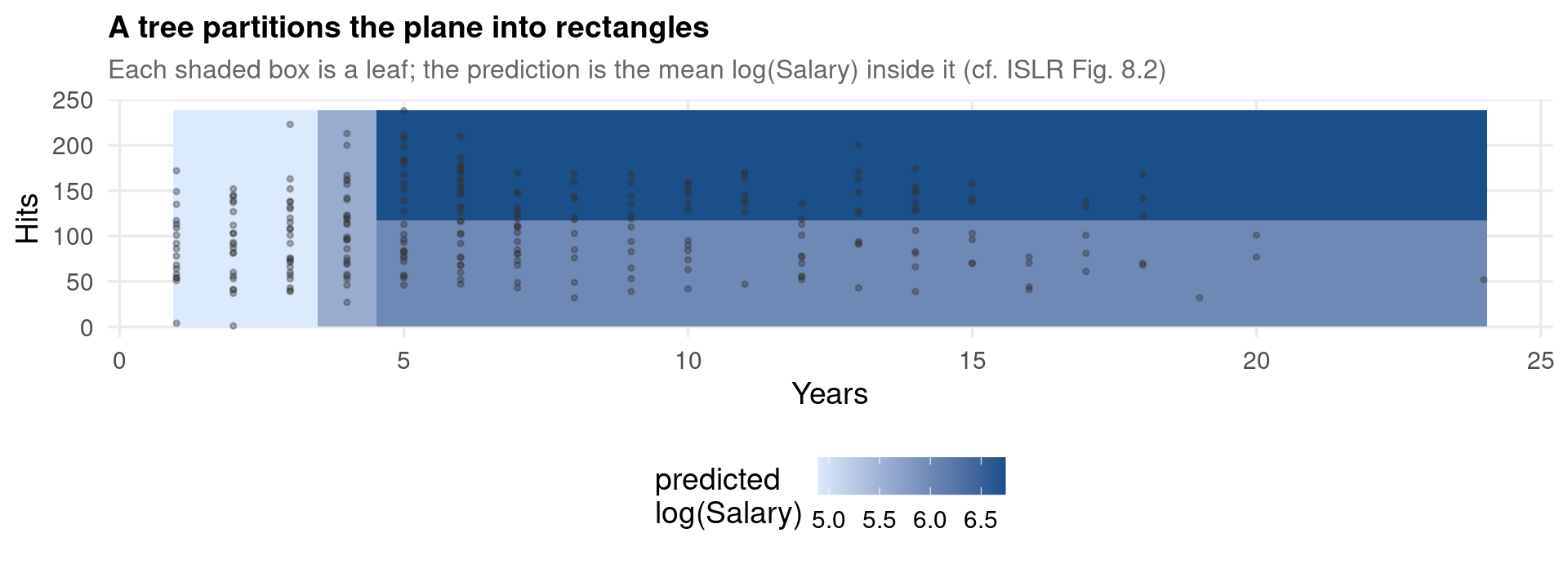
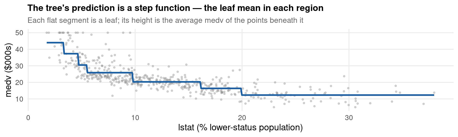
Time Series — What to Watch

  • One-step vs multi-step. Recursive forecasts feed predictions back as inputs; errors compound. Or train a separate model per horizon (direct).
  • Leakage hides everywhere. Rolling means, scalers, and feature selection must be fit on the training window only.
  • Trees don’t extrapolate. Difference or detrend; never feed a raw trending level as the target.
  • Beat a real benchmark. Random walk and a simple AR are hard to beat — report them.

What Trees Add — and What They Still Lack

Over regularised (linear) regression, trees and ensembles give us:

  • No linearity assumption\(g(\mathbf{x})\) can be arbitrarily non-linear.
  • Automatic interactions — experience × occupation, rooms × neighbourhood, found without pre-specification.
  • Mixed inputs, no scaling — continuous, binary, and categorical predictors handled natively.
  • Honest accuracy for free — OOB error estimates test error at no extra cost.
  • Built-in regularisation (XGBoost) — the \(\ell_1+\ell_2\) leaf penalties are the Lasso/Ridge ideas, one level down.
  • No coefficients — a tree predicts; it does not estimate a structural parameter. Inference needs the partial-out wrapper.
  • No causal guarantee — a better nuisance does not by itself deliver a causal \(\hat\beta\); conditional independence is still required.
  • Interpretability cost — the nuisance is a black box; SHAP and PDP describe the fit, not the world.
  • Heterogeneity averaged away — one \(\hat\beta^{\text{union}}\) hides variation (→ causal forests).
  • Tuning burden (boosting) — XGBoost can overfit and needs early stopping a forest does not.

The honest summary. Trees do not replace econometrics — they upgrade its nuisance step. The estimator of interest stays low-dimensional and interpretable; the machine learning lives entirely in \(\hat g(\mathbf{x})\) and \(\hat m(\mathbf{x})\).

Pitfalls — What to Report

There is no coefficient table — so what do you report? A credible tree-based write-up states:

Item What to report
Task Prediction, screening, or DML nuisance — say which
Validation Held-out test set or \(K\)-fold CV; the seed; the split
Accuracy Out-of-sample RMSE/\(R^2\) vs OLS / Lasso / Ridge benchmarks
Importance Permutation importance (not impurity); SHAP for direction
Tuning mtry (forest); eta, max_depth, early-stopping round (XGBoost)
Causal target Partial-out \(\hat\beta\) with robust SE, and the cross-fitting scheme

Match the tool to the goal. Best prediction → XGBoost (or a forest, more robustly). Screening controls → forest permutation importance / SHAP. One causal coefficient → tree partial-out / DML with cross-fitting. Heterogeneous effects → causal forest. An interpretable policy model → a small pruned tree or a sparse Lasso.

Pitfalls — The Recurring Mistakes

  1. Reading a raw tree prediction, importance, or SHAP value as a causal effect. They rank and describe prediction; causation needs the partial-out / DML step and an identification argument.
  2. Forming residuals from in-sample tree fits. Overfitting bias leaks into \(\hat\beta\) and pulls it toward zero. Always use OOB or cross-fitted predictions.
  3. Running XGBoost with a fixed number of rounds. Without early stopping it overfits — and a forest would have been the safer default.
  4. Reporting training \(R^2\). As with high-dimensional regression, training fit is meaningless; only out-of-sample error counts.
  5. Tuning on the test set. Choose hyperparameters by inner CV, then touch the test set exactly once.

A coding pitfall, too. In Python, a bare plotting call (e.g. ax.plot(...)) returns artist objects that print as [<matplotlib.lines.Line2D ...>]. Suppress them: assign to _ (_ = ax.plot(...)) and end the chunk with plt.show(). Every Python chunk in this deck follows that rule.

References — Methods

Foundational — trees and ensembles

Trees for causal inference

Econometric perspective

References — Textbooks, Tutorials & Multi-Language Resources

Core textbooks

Hands-on, across the three environments

  • Boehmke & Greenwell (2020). Hands-On Machine Learning with R. Chapman & Hall/CRC — trees, bagging, RF, GBM/XGBoost, stacking, and interpretability (PDP, ICE, SHAP). bradleyboehmke.github.io/HOML
  • Géron (2022). Hands-On Machine Learning with Scikit-Learn, Keras & TensorFlow, 3rd ed. O’Reilly — the Python counterpart.
  • Cerulli (2023). Fundamentals of Supervised Machine Learning: With Applications in Python, R, and Stata. Springer — trees & ensembles side-by-side in all three languages. doi:10.1007/978-3-031-41337-7
  • Molnar (2022). Interpretable Machine Learning, 2nd ed. — concept reference for permutation importance, PDP, ICE, LIME, SHAP. christophm.github.io/interpretable-ml-book

Causal ML — tutorials & software

  • Golub Capital Social Impact Lab (2023). Machine Learning-based Causal Inference Tutorial (R; AIPW, RATE, policy learning). bookdown.org/stanfordgsbsilab/ml-ci-tutorial
  • Facure (2023). Causal Inference in Python. O’Reilly — Python DML/CATE. matheusfacure.github.io/python-causality-handbook
  • R: grf, policytree (Athey, Tibshirani, Wager, Sverdrup). Python: EconML (Microsoft Research / PyWhy), doubleml. Stata: ddml, pystacked (Ahrens, Hansen, Schaffer & Wiemann 2023).

Packages & data used here

  • ranger (doi:10.18637/jss.v077.i01), rpart, xgboost, SHAPforxgboost. Datasets Hitters, Boston (ISLR2); wagepan (wooldridge).
  • Companion deck: machine-learning-regularisation-in-econometrics.Qmd (Lasso, Ridge, Elastic Net, full DML).

Exercises

  1. Pruning (Hitters). Grow a depth-4 tree of log(Salary) on all predictors, then prune it by 10-fold CV and the 1-SE rule. Does it keep Years and Hits on top? Compare its test RMSE to the depth-2 tree from the slide.
  2. Tuning mtry (Boston). Fit forests with mtry \(\in\{2,4,6,8,12\}\) and record the OOB MSE. Which value minimises it, and how does it compare to the default \(p/3=4\)? Plot OOB MSE against mtry.
  3. Forest vs boosting (Boston). On a fixed 50/50 split, compare the test RMSE of a forest and an early-stopped XGBoost. At which round does the XGBoost test error stop improving?
  4. Importance agreement (Boston). Compute permutation importance and mean \(|\)SHAP\(|\) for the same model. Do both rank lstat and rm on top? Where do they disagree, and why might impurity importance differ again?
  5. Overfitting bias (wagepan). Re-estimate the RF partial-out premium twice: once with in-sample forest predictions, once with OOB predictions. How much does \(\hat\beta^{\text{union}}\) move, and in which direction? Explain the bias.
  6. Stability in \(B\) (wagepan). Re-run the RF and XGBoost partial-out with num.trees / n_estimators \(\in\{100, 500, 1000\}\). At what ensemble size does the premium stabilise to three decimals?
  7. ICE vs PDP (Boston). Plot ICE curves for lstat from the boosted model. Are they parallel (homogeneous effect) or do they fan out (interaction)? Centre the curves at their left end (c-ICE) and re-examine. What does this imply for trusting the PDP?
  8. Policy learning (any treatment dataset). From a causal forest, build doubly-robust (AIPW) scores and fit a depth-2 policy_tree (R) or PolicyTree (Python). Write out the resulting treatment rule in words, and compare its estimated value to “treat everyone” and “treat no one”.

Thank You

Athanassios Stavrakoudis
Applied Informatics and Computational Economics Lab
Department of Economics
University of Ioannina
Greece

astavrak@uoi.gr  ·  linkedin.com/in/astavrakoudis