Part 1 — Why simulate macro-finance? the equity premium puzzle on 2026 data, the SDF, Hansen–Jagannathan bounds
Part 2 — The simulation toolkit Tauchen & Rouwenhorst, SDE discretisation, variance reduction
Part 3 — Consumption-based asset pricing Lucas tree, Epstein–Zin, long-run risk, habit, rare disasters
Part 4 — Solving & simulating a DSGE Blanchard–Kahn, perturbation, risk premia, the financial accelerator
Part 5 — Term structure simulation Vasicek, CIR, Nelson–Siegel, the GSW curve, bond scenarios
Part 6 — Macro-financial risk Growth-at-Risk, regime switching, scenario and tail simulation
Part 7 — Estimation by simulation SMM, indirect inference, weak identification, small samples
Part 8 — Practice & exercises reporting checklist, pitfalls, exercises, further reading
Every part runs the same loop:
Write the model down solve it simulate it compute the moments it implies put those beside the same moments in 2026-vintage US data say where the model wins and where it does not.
Two deliberate departures from the standard slide order used in this lecture series. Both are choices, not drift.
1. The motivating puzzle comes before the literature review. Nobody cares which papers solved the equity premium puzzle until they have watched it happen on data that ends this year. Required Packages still comes first.
2. The tests are distributed, not collected in one section. This deck uses seven of them — Ljung–Box on simulated against actual series, the Blanchard–Kahn rank condition, the Feller condition, Hansen’s \(J\), the Hamilton likelihood-ratio test for regimes, a quantile-crossing check, and Diebold–Mariano on Growth-at-Risk densities. Each belongs beside the stage it validates.
This deck is about simulation as the engine: solving stochastic macro-finance models, simulating them, and holding the simulations to account against data.
Owned by another deck
Where the boundary is touched here
Monte Carlo Methods — MC as an estimator and test-design tool
Part 2 recaps the \(1/\sqrt{B}\) law in one slide, then covers variance reduction, which that deck does not
Part 5 uses a Kalman filter for dynamic Nelson–Siegel; it is cited, not re-derived
DCC-GARCH-Copula — conditional volatility, dependence, VaR backtesting, CoVaR
Part 6 does macro-financial risk; systemic risk is one cross-reference
Structural Estimation — GMM, SMM and indirect inference theory
Part 7 applies both to a macro-finance model
Numerical Applications — floating point, decompositions, optimisation, ODEs
Part 2 uses those tools; SDE simulation is new
VAR & Local Projections — VAR, SVAR, LP as estimators
Part 4 uses lpirf to confront model IRFs with empirical ones
68 content slides is three to four sittings, not one. The core path below is 55 of them, in order, grouped into four sessions. The other 13 are reference depth: they earn their place, but they are scrollable deep dives that read better after class than during it. Seven of those carry a visible reference depth tag on the slide itself.
Session 1 — Parts 1 & 2 · the puzzle and the toolkit Core (12). Equity Premium Puzzle on 2026 Data → Puzzle Code → Puzzle Results & Interpretation → SDF and the Hansen–Jagannathan Bound → The Data → DGP Mathematical Specification → DGP Code Implementation → Discretising a Persistent AR(1) → Tauchen & Rouwenhorst Code → Simulating in Continuous Time → Discretisation Bias → Monte Carlo Error, Burn-in & Variance Reduction Reference (4). Four Stylised Facts · DGP Diagnostics · Accuracy vs Persistence · Variance Reduction Code
Session 2 — Part 3 · consumption-based asset pricing Core (9). The Lucas Tree → Lucas Tree Code → Lucas Tree Results → Epstein–Zin → Long-Run Risks → Long-Run Risks Results & Fragility → Habit Formation → Rare Disasters & the Peso Problem → Model Horse Race Reference (1). Long-Run Risks Code
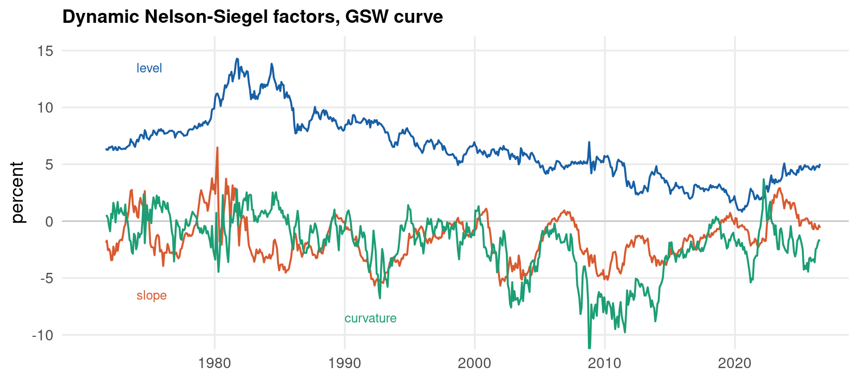
Session 3 — Parts 4 & 5 · solving models, pricing bonds Core (14). The Model → Log-Linearisation & Blanchard–Kahn → First-Order Perturbation Code → Simulating the Solved Model → Stochastic Simulation & Model Moments → Why First Order Kills the Risk Premium → Second Order: the Risk Correction → Financial Frictions → Affine Term Structure Models → Vasicek & CIR → Simulated vs Actual GSW Curves → Estimating the Short-Rate Process → Nelson–Siegel–Svensson & the GSW Parameters → Scenario Simulation for a Bond Portfolio Reference (4). Financial Accelerator vs BAA-10Y · Model IRFs vs Local Projections · From Short Rate to Yield Curve · Dynamic Nelson–Siegel
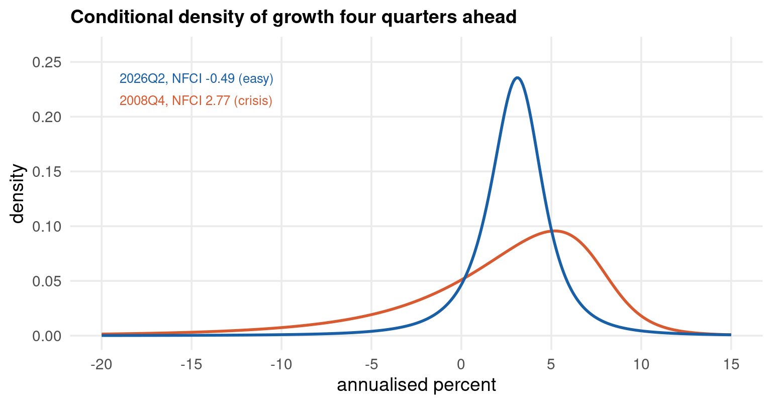
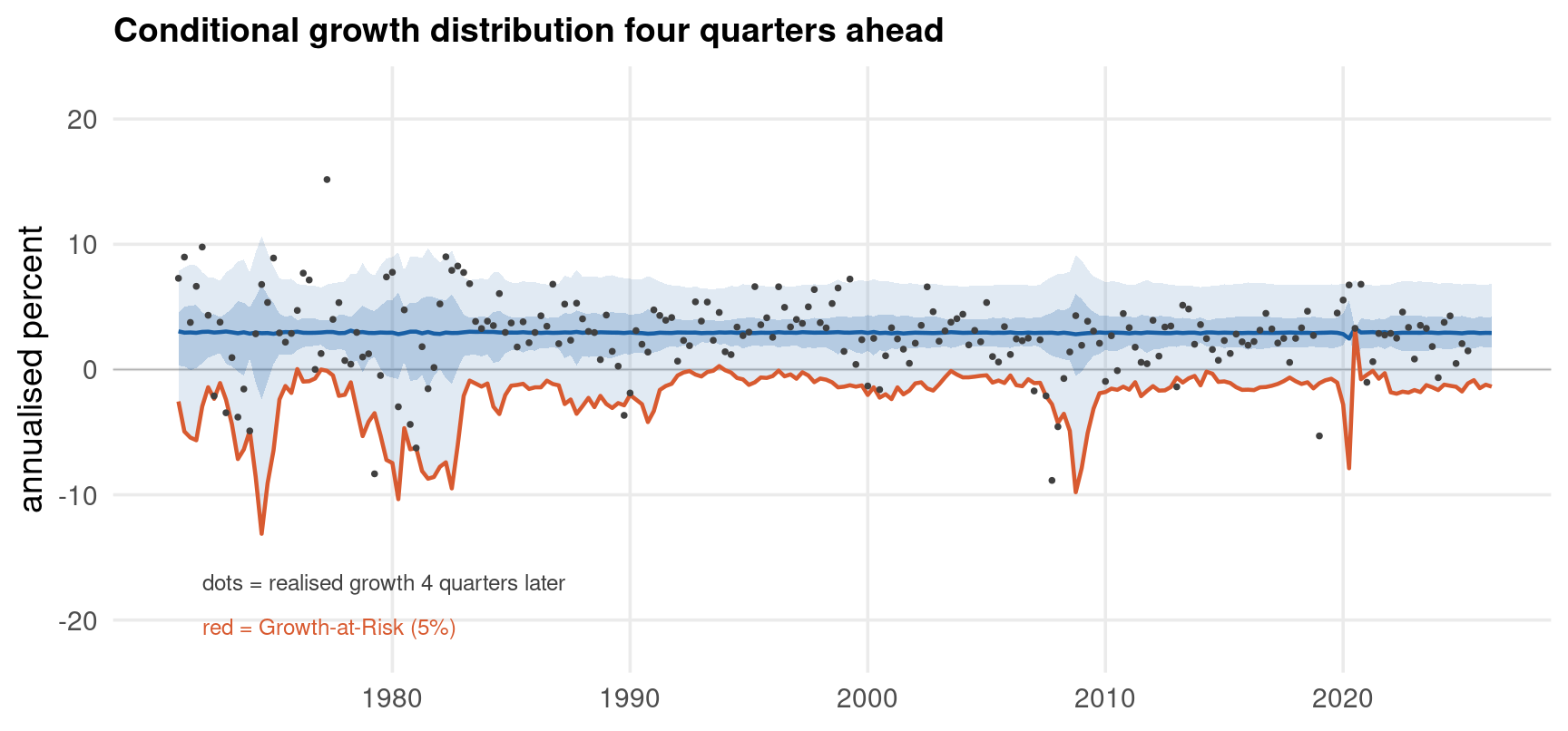
Session 4 — Parts 6, 7 & 8 · risk, estimation, practice Core (20). Growth-at-Risk → GaR Quantile Regression → The Predictive Density → GaR Fan Chart → Regime Switching → Simulating Macro Scenarios → Simulated Method of Moments → SMM Recovering Known Truth → SMM Does It Recover the Truth? → SMM on a Noisy Objective (CRN) → Indirect Inference → Weak Identification → A Century Is Not Enough → Model Comparison → What This Deck Found → What to Report → Common Pitfalls → Exercises (Simulation & Estimation) → Exercises (Testing & Diagnostics) → Further Reading Reference (4). Regime Switching Code · Tail Simulation & Importance Sampling · Reproducibility & Computation · Variations & Method Chooser
Required Packages
library(QZ) # qz.dgges() — generalized Schur; the Blanchard-Kahn solutionlibrary(sn) # dst(), rst() — skew-t densities for Growth-at-Risklibrary(quantreg) # rq() — quantile regressionlibrary(randtoolbox) # sobol() — quasi-Monte Carlo sequenceslibrary(vars) # VAR(), irf() — scenario simulation, auxiliary modelslibrary(tseries) # adf.test(), jarque.bera.test()library(expm) # %^% — matrix powers for Markov chains and IRFslibrary(future.apply) # future_lapply() — parallel Monte Carlolibrary(tidyverse) # data wrangling & ggplot2library(png) # readPNG() — reload Stata-exported graphs
import numpy as np # arrays, linear algebraimport pandas as pd # data frames, CSV inputimport scipy.stats as st # distributions, skew-t, KDEfrom scipy.linalg import ordqz # generalized Schur — DSGE solutionfrom scipy.optimize import minimize # SMM, indirect inference, MLEfrom scipy.stats import qmc # Sobol sequencesimport statsmodels.api as sm # quantile regression, VAR, state spacefrom statsmodels.tsa.regime_switching.markov_regression import MarkovRegressionimport matplotlib.pyplot as plt # all figures
* Nothing to install: every command used here ships with Stata SE 19.dsge // linear DSGE: solve, simulate, estimatedsgenl // nonlinear DSGE, log-linearised around the steady statesspace // state-space models — dynamic Nelson-Siegelmswitch // Markov-switching mean and varianceqreg// quantile regression — Growth-at-Riskvar, irf// scenario simulation, auxiliary modelslpirf // Jorda local projections — Part 4mata// Tauchen, SDE paths, bond pricing, SMM via optimize()
Three routines have no Stata counterpart and the relevant tab says so rather than being dropped: Sobol sequences (Part 2), Epstein–Zin and habit preferences (Part 3), and the skew-t predictive density (Part 6).
Part 1 — Why Simulate Macro-Finance?
The equity premium puzzle on 2026 data, the stochastic discount factor, Hansen-Jagannathan bounds, and the five simulated laboratories.
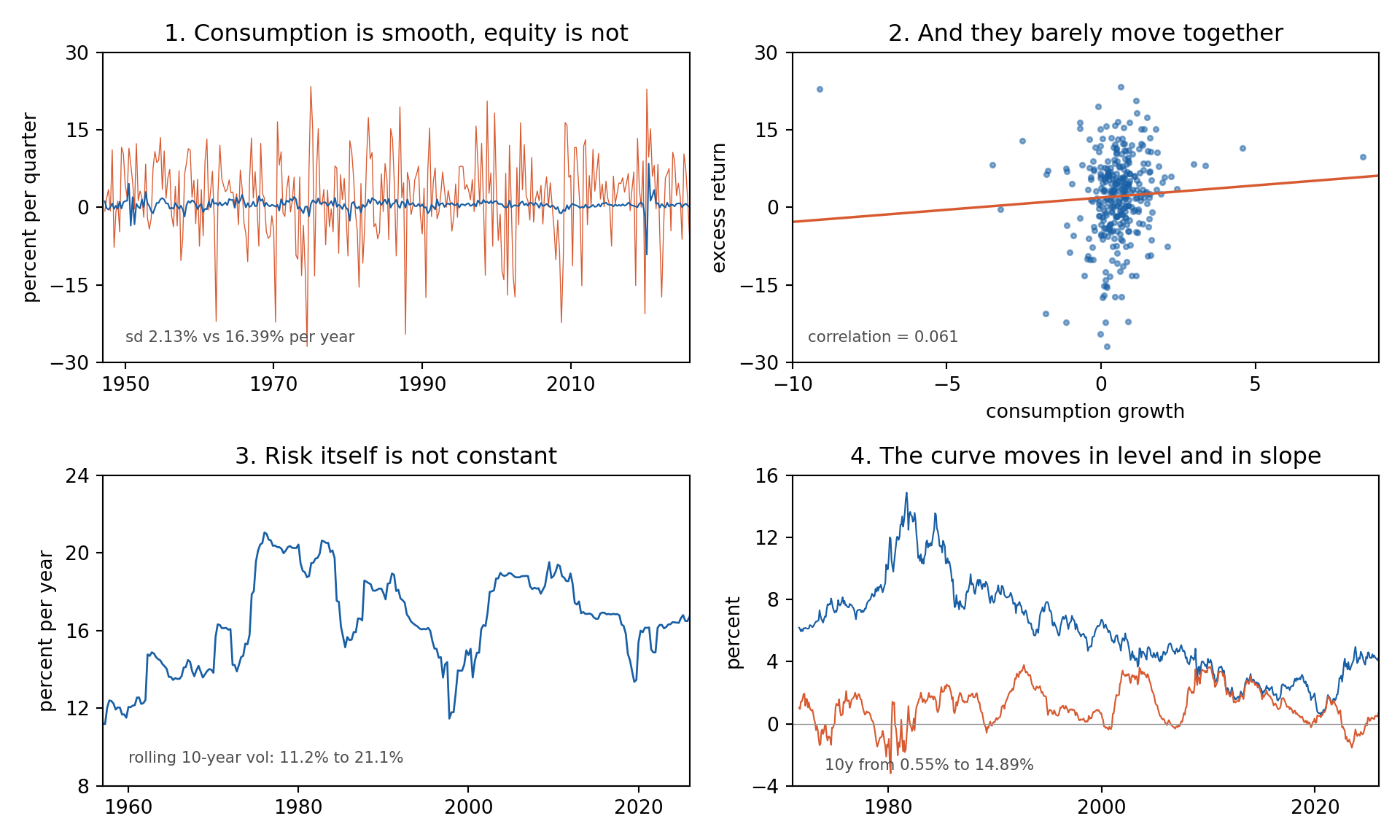
Two facts about the United States, measured on data that ends this year:
holding the market rather than a Treasury bill has paid about 8.6% a year, with a standard deviation of 16.4%
aggregate consumption per head has grown at 2.1% a year, with a standard deviation of 2.1%
Consumption is eight times smoother than the asset whose risk it is supposed to price. Worse, the two barely move together — their correlation is \(0.06\).
A representative investor with standard preferences buys stocks only to the extent that stocks pay badly when consumption is low. If stocks and consumption are almost unrelated, stocks are almost riskless to that investor, and she should demand almost no premium for holding them.
The market pays 8.6% a year for a risk that, measured through consumption, is barely there. That gap is the equity premium puzzle — and it is the reason the rest of this deck simulates models rather than estimating regressions.
The consumer’s first-order condition for any gross return \(R_{t+1}\):
Everything on the left and the covariance on the right are measured. Only \(\gamma\) is free. The slide after next solves for it.
The Equity Premium Puzzle — Code
Monthly market factors are compounded to quarterly and merged with quarterly consumption growth, so returns and consumption are measured over the same interval. Common sample: 1947Q2 to 2026Q2, 317 quarters.
Code
eq <-read.csv("../data/mfsim-equity.csv")ma <-read.csv("../data/mfsim-macro.csv")# Monthly returns compound to quarterly through the sum of their logseq <- eq |>mutate(qtr =sprintf("%sQ%d", substr(date, 1, 4), (as.integer(substr(date, 6, 7)) -1) %/%3+1),lm =log(1+ (mktrf + rf) /100),lf =log(1+ rf /100))agg <-aggregate(cbind(lm, lf) ~ qtr, data = eq, FUN = sum) |>mutate(re =exp(lm) -exp(lf))d <-merge(agg, ma[, c("qtr", "dcons")], by ="qtr") |>mutate(dc = dcons /400) # dcons is 400 x log-difference# Annualised moments: means x 4, volatilities x sqrt(4)mre <-mean(d$re); sre <-sd(d$re)mdc <-mean(d$dc); sdc <-sd(d$dc)gamma_euler <- mre /cov(d$dc, d$re)
Sample: 1947Q2 to 2026Q2 n = 317 quarters
                 Quantity       Value
      Excess return, mean  8.61% / yr
        Excess return, sd 16.39% / yr
             Sharpe ratio       0.525
 Consumption growth, mean  2.08% / yr
   Consumption growth, sd  2.13% / yr
      Correlation(dc, Re)       0.061
       Covariance(dc, Re)   5.352e-05
    Implied risk aversion         402
Code
import numpy as npimport pandas as pdeq = pd.read_csv("../data/mfsim-equity.csv")ma = pd.read_csv("../data/mfsim-macro.csv")# Monthly returns compound to quarterly through the sum of their logseq["qtr"] = (eq["date"].str[:4] +"Q"+ (((eq["date"].str[5:7].astype(int) -1) //3) +1).astype(str))eq["lm"] = np.log(1+ (eq["mktrf"] + eq["rf"]) /100)eq["lf"] = np.log(1+ eq["rf"] /100)agg = eq.groupby("qtr", as_index=False)[["lm", "lf"]].sum()agg["re"] = np.exp(agg["lm"]) - np.exp(agg["lf"])d = agg.merge(ma[["qtr", "dcons"]], on="qtr")d["dc"] = d["dcons"] /400# dcons is 400 x log-differencemre, sre = d["re"].mean(), d["re"].std(ddof=1)mdc, sdc = d["dc"].mean(), d["dc"].std(ddof=1)cv = np.cov(d["dc"], d["re"], ddof=1)[0, 1]gamma_euler = mre / cvout = (f"Sample: {d['qtr'].min()} to {d['qtr'].max()} n = {len(d)} quarters\n\n"f"Excess return, mean {400*mre:10.2f}% / yr\n"f"Excess return, sd {200*sre:10.2f}% / yr\n"f"Sharpe ratio {2*mre/sre:10.3f}\n"f"Consumption growth, mean {400*mdc:10.2f}% / yr\n"f"Consumption growth, sd {200*sdc:10.2f}% / yr\n"f"Correlation(dc, Re) {np.corrcoef(d['dc'], d['re'])[0,1]:10.3f}\n"f"Covariance(dc, Re) {cv:10.3e}\n"f"Implied risk aversion {gamma_euler:10.0f}")import sys; nchars = sys.stdout.write(out +"\n"); sys.stdout.flush()
Sample: 1947Q2 to 2026Q2   n = 317 quarters

Excess return, mean              8.61% / yr
Excess return, sd               16.39% / yr
Sharpe ratio                    0.525
Consumption growth, mean         2.08% / yr
Consumption growth, sd           2.13% / yr
Correlation(dc, Re)             0.061
Covariance(dc, Re)          5.352e-05
Implied risk aversion             402
Code
quietly import delimited "../data/mfsim-equity.csv", clear stringcols(2)* Monthly returns compound to quarterly through the sumof their logsgenerate qtr = substr(date,1,4) + "Q" + string(int((real(substr(date,6,2))-1)/3) + 1, "%1.0f")generate lm = ln(1 + (mktrf + rf)/100)generate lf = ln(1 + rf/100)collapse (sum) lm lf, by(qtr)generate re = exp(lm) - exp(lf)tempfileeqquietlysave`eq'quietly import delimited "../data/mfsim-macro.csv", clear stringcols(3)keep qtr dconsquietlymerge 1:1 qtr using`eq', keep(match) nogenerategenerate dc = dcons/400quietlysummarize rescalar mre = r(mean)scalar sre = r(sd)quietlysummarize dcscalar mdc = r(mean)scalar sdc = r(sd)quietly correlate dc re, covariancescalar cv = r(cov_12)quietly correlate dc rescalar rho = r(rho)* One display command, so the table prints as one blockdisplay"n = " _N " quarters"_newline///_newline///"Excess return, mean " %10.2f 400*mre " % / yr"_newline///"Excess return, sd " %10.2f 200*sre " % / yr"_newline///"Sharpe ratio " %10.3f 2*mre/sre _newline///"Consumption growth, mean " %10.2f 400*mdc " % / yr"_newline///"Consumption growth, sd " %10.2f 200*sdc " % / yr"_newline///"Correlation(dc, Re) " %10.3f rho _newline///"Covariance(dc, Re) " %10.3e cv _newline///"Implied risk aversion " %10.0f mre/cv
n = 317 quarters

Excess return, mean             8.61 % / yr
Excess return, sd              16.39 % / yr
Sharpe ratio                   0.525
Consumption growth, mean        2.08 % / yr
Consumption growth, sd          2.13 % / yr
Correlation(dc, Re)            0.061
Covariance(dc, Re)         5.352e-05
Implied risk aversion            402
Sample 1947Q2–2026Q2, 317 quarters. Over the full 1926–2026 monthly sample the premium is 8.36% with a Sharpe ratio of 0.455 — the puzzle is not an artefact of the postwar window.
\(\gamma = 402\) is not a preference parameter, it is a rejection. Survey and experimental evidence puts risk aversion in the low single digits. Values above about 10 imply behaviour nobody displays: at \(\gamma = 402\) an agent would pay almost any premium to avoid a coin flip over 1% of consumption.
The arithmetic is driven by the correlation of 0.061, not by the premium. Because
a near-zero \(\rho\) makes the covariance vanish, and \(\gamma\) must explode to keep \(E[R^e] = \gamma \, \mathrm{Cov}(\Delta c, R^e)\) in balance. Equities are not risky in the consumption metric. Any model that solves the puzzle has to make them risky some other way — that is what Part 3 is for.
Raising \(\gamma\) to rescue the premium breaks a second equation. For lognormal consumption growth the model’s own risk-free rate is
With \(\beta = 0.99\) per quarter, at the values just measured:
\(\gamma\)
model \(r^f\)
2
8.09% / yr
16.6
32.27% / yr
402
\(-2837\%\) / yr
The actual ex-post real policy rate over the same sample is 1.42% / yr.
Even \(\gamma = 2\) — far too low for the premium — already predicts a risk-free rate six times too high. This is Weil’s risk-free rate puzzle, and it means the two puzzles cannot be traded off against each other.
The previous slide assumed a particular discount factor and asked what \(\gamma\) would have to be. Hansen and Jagannathan (1991) turn the question around and ask something far more useful for a simulator:
Forget preferences. What must be true of any discount factor that prices these returns, whatever model produced it?
The answer is a lower bound on how volatile the discount factor has to be, set entirely by the Sharpe ratio of the assets:
A high Sharpe ratio in the data is a demand for a volatile \(M\) — and \(M\) is the one object every model in Parts 3 to 5 produces. That makes this the cheapest validation check a simulated model will ever face: simulate, compute two moments of \(M\), plot the point, see whether it clears the line. No estimation, no standard errors, no auxiliary assumptions.
For CRRA preferences under lognormal consumption growth the left-hand side is approximately \(\gamma \sigma_{\Delta c}\), which yields the textbook rule of thumb
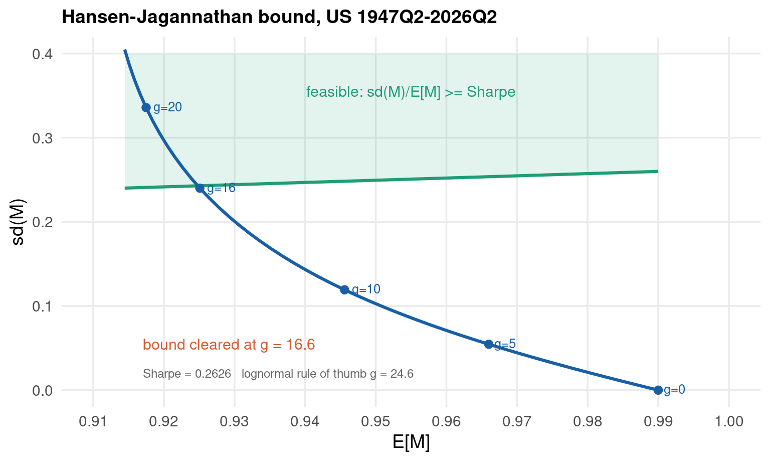
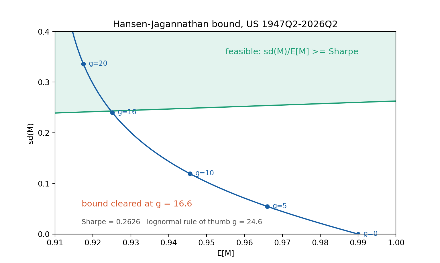
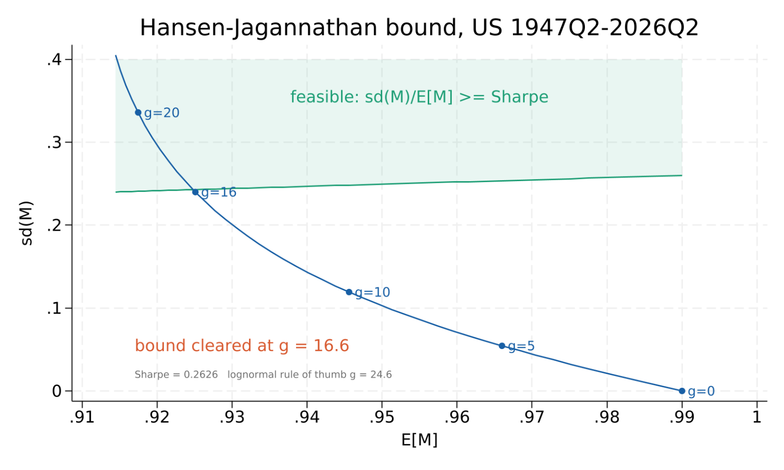
Two ways to compute it, and they disagree. The lognormal rule of thumb demands \(\gamma \ge 24.6\); the exact bound, computed on the consumption data as it actually is, is cleared at \(\gamma = 16.6\). Consumption growth has fatter tails than a lognormal — 2020Q2 alone is \(-36.5\%\) at an annual rate — and those tails make \(\exp(-\gamma \Delta c)\) more volatile than the approximation allows. Neither number is remotely defensible as a preference parameter, but a model builder should quote the one computed from the data.
The code tabs compute both. The feasible region is everything on or above the ray of slope \(\text{Sharpe} = 0.2626\) (quarterly); the curve traces CRRA discount factors \(M = \beta \exp(-\gamma \Delta c)\) built from the actual consumption data, for \(\gamma\) from 0 to 22.
Where the bound comes from
Expanding \(E[MR^e] = 0\) and applying Cauchy–Schwarz to the covariance it leaves behind gives
\[\mathrm{Cov}\!\left( M, R^e \right) = -E[M]\,E\!\left[ R^e \right], \qquad \left| \mathrm{Cov}\!\left( M, R^e \right) \right| \le \sigma(M)\,\sigma\!\left( R^e \right)\]
Divide the second by the first and the bound falls out, with no preference parameter anywhere in the argument.
Code
beta_q <-0.99sharpe <-mean(d$re) /sd(d$re) # quarterly Sharpe ratio# CRRA locus: one (E[M], sd(M)) point per level of risk aversiongammas <-seq(0, 22, by =0.5)locus <-data.frame(gamma = gammas) |>mutate(EM =sapply(gamma, \(g) mean(beta_q *exp(-g * d$dc))),sdM =sapply(gamma, \(g) sd(beta_q *exp(-g * d$dc))))# Where does the locus first clear the bound?gap <- \(g) sd(beta_q *exp(-g * d$dc)) /mean(beta_q *exp(-g * d$dc)) - sharpegamma_hj <-uniroot(gap, c(1, 25))$rootgamma_ln <- sharpe /sd(d$dc) # the lognormal rule of thumbggplot(locus) +aes(x = EM, y = sdM) +geom_ribbon(aes(ymin = sharpe * EM, ymax =0.40), fill ="#1D9E75", alpha =0.12) +geom_line(aes(y = sharpe * EM), colour ="#1D9E75", linewidth =1.1) +geom_line(colour ="#185FA5", linewidth =1.1) +geom_point(data =subset(locus, gamma %in%c(0, 5, 10, 16.5, 20)),colour ="#185FA5", size =2.4) +coord_cartesian(xlim =c(0.91, 1.00), ylim =c(0, 0.40))
quarterly Sharpe 0.2626
exact bound cleared at gamma = 16.6
lognormal rule of thumb gamma = 24.6
Code
import matplotlib.pyplot as pltfrom scipy.optimize import brentqbeta_q =0.99sharpe = d["re"].mean() / d["re"].std(ddof=1)dc = d["dc"].to_numpy()def moments(g): m = beta_q * np.exp(-g * dc)return m.mean(), m.std(ddof=1)gammas = np.arange(0, 22.5, 0.5)EM = np.array([moments(g)[0] for g in gammas])sdM = np.array([moments(g)[1] for g in gammas])gamma_hj = brentq(lambda g: moments(g)[1] / moments(g)[0] - sharpe, 1, 25)gamma_ln = sharpe / dc.std(ddof=1)fig, ax = plt.subplots(figsize=(8, 4.8))xs = np.linspace(0.91, 1.00, 50)ax.fill_between(xs, sharpe * xs, 0.40, color="#1D9E75", alpha=0.12)ax.plot(xs, sharpe * xs, color="#1D9E75", lw=1.6)ax.plot(EM, sdM, color="#185FA5", lw=1.6)for g in [0, 5, 10, 16.5, 20]: e, s = moments(g) ax.plot(e, s, "o", color="#185FA5", ms=5) ax.annotate(f"g={g:.0f}", (e, s), textcoords="offset points", xytext=(7, -2), color="#185FA5", fontsize=9)ax.text(0.955, 0.355, "feasible: sd(M)/E[M] >= Sharpe", color="#1D9E75", fontsize=11)ax.text(0.917, 0.055, f"bound cleared at g = {gamma_hj:.1f}", color="#D85A30", fontsize=11)ax.text(0.917, 0.020,f"Sharpe = {sharpe:.4f} lognormal rule of thumb g = {gamma_ln:.1f}", color="#555555", fontsize=9)axopts = ax.set(xlim=(0.91, 1.00), ylim=(0, 0.40), xticks=np.arange(0.91, 1.001, 0.01), yticks=np.arange(0, 0.41, 0.10), xlabel="E[M]", ylabel="sd(M)", title="Hansen-Jagannathan bound, US 1947Q2-2026Q2")plt.show()
Code
quietly import delimited "../data/mfsim-equity.csv", clear stringcols(2)generate qtr = substr(date,1,4) + "Q" + string(int((real(substr(date,6,2))-1)/3) + 1, "%1.0f")generate lm = ln(1 + (mktrf + rf)/100)generate lf = ln(1 + rf/100)collapse (sum) lm lf, by(qtr)generate re = exp(lm) - exp(lf)tempfileeqquietlysave`eq'quietly import delimited "../data/mfsim-macro.csv", clear stringcols(3)keep qtr dconsquietlymerge 1:1 qtr using`eq', keep(match) nogenerategenerate dc = dcons/400quietlysummarize rescalar sharpe = r(mean)/r(sd)quietlysummarize dcscalar sdc = r(sd)scalar gamma_ln = sharpe/sdc* Bisection for the exact crossing -- the same root R finds with uniroot()scalar lo = 1scalar hi = 25forvalues it = 1/60 {scalar mid = (lo + hi)/2quietlygeneratedouble mtmp = 0.99*exp(-mid*dc)quietlysummarize mtmpscalarratio = r(sd)/r(mean)quietlydrop mtmpif (ratio < sharpe) scalar lo = midelsescalar hi = mid}scalar gamma_hj = (lo + hi)/2* One (E[M], sd(M)) point per levelof risk aversiontempfile locustempname locpostfile`loc'gamma em sdm using`locus'forvalues j = 0/44 {local g = `j' * 0.5quietlygeneratedouble mtmp = 0.99*exp(-`g'*dc)quietlysummarize mtmppost`loc' (`g') (r(mean)) (r(sd))quietlydrop mtmp}postclose`loc'quietlyuse`locus', cleargenerate bound = sharpe * emgenerate top = 0.40* Markers at a few levelsof risk aversion, asin the R and Python tabsgeneratebyte mark = abs(gamma-0) < 0.01 | abs(gamma-5) < 0.01 | ///abs(gamma-10) < 0.01 | abs(gamma-16.5) < 0.01 | ///abs(gamma-20) < 0.01generate mem = em if markgenerate msd = sdm if markgenerate str8 glab = "g=" + string(gamma, "%2.0f") if marklocal t1 "feasible: sd(M)/E[M] >= Sharpe"local t2 = "bound cleared at g = " + string(gamma_hj, "%3.1f")local t3 = "Sharpe = " + string(sharpe, "%5.4f") + ///" lognormal rule of thumb g = " + string(gamma_ln, "%3.1f")twoway (rarea top bound em, color("29 158 117%12") lwidth(none)) /// (line bound em, sort lcolor("29 158 117") lwidth(medium)) /// (line sdm em, sort lcolor("24 95 165") lwidth(medium)) /// (scatter msd mem, mcolor("24 95 165") msymbol(circle) ///mlabel(glab) mlabcolor("24 95 165") mlabposition(3) ///mlabsize(small)), ///xscale(range(0.91 1.00)) yscale(range(0 0.40)) ///xlabel(0.91(0.01)1.00) ylabel(0(0.10)0.40) ///xtitle("E[M]") ytitle("sd(M)") ///title("Hansen-Jagannathan bound, US 1947Q2-2026Q2") ///text(0.355 0.955 "`t1'", color("29 158 117") size(medsmall)) ///text(0.055 0.917 "`t2'", color("216 90 48") size(medsmall) /// placement(e) justification(left)) ///text(0.020 0.917 "`t3'", color(gs7) size(vsmall) /// placement(e) justification(left)) ///legend(off) graphregion(color(white))graphexport"../plots/mfsim-hj-stata.png", replacewidth(1600)
Part 5 — a curve to fit, and the Nelson–Siegel–Svensson parameters behind it
mfsim-daily.csv
S&P 500, VIX, 10-year yield, credit spread
Part 6 — daily risk measures and scenario inputs
mfsim-lucas.csv
Lucas tree endowment economy
Part 3 — a model whose answer is known in closed form
mfsim-lrr.csv
Bansal–Yaron long-run risk
Parts 3 and 7 — a latent state nobody observes
mfsim-dsge.csv
log-linear RBC with a finance premium
Parts 4 and 7 — known deep parameters to recover
mfsim-term.csv
Vasicek and CIR paths + implied curves
Parts 2 and 5 — exact transitions, so discretisation error is measurable
mfsim-regime.csv
two-state Markov-switching growth
Part 6 — a regime the filter has to find
            Dataset  Obs       From         To                       Headline
   equity (monthly) 1199    1926-07    2026-05 excess ret 8.36%/yr, sd 18.39%
  macro (quarterly)  317     1947Q2     2026Q2 cons growth 2.08%/yr, sd 2.13%
 yields (month-end)  660    1971-08    2026-07       10y from 0.55% to 14.89%
              daily 2492 2016-08-02 2026-07-30           VIX from 9.1 to 82.7
The consumption number is the one people misread. The column dcons is \(400 \times\) the log difference — an annualised growth rate, not a level. Its own standard deviation (4.27) is therefore not a volatility. Divide by 400 for quarterly log growth, then annualise the standard deviation by \(\sqrt{4}\):
Everything here ends in 2026. That is the point of rebuilding rather than reusing a textbook table.
Source
Latest observation
Note
Ken French factors
2026-05
built from the 202605 CRSP database
GSW zero-coupon curve
2026-07-24
daily since 1961; the Fed Board revises it as new data arrive
FRED macro
2026Q2
GDP and consumption are revised for years after first release
FRED daily
2026-07-30
Three honest warnings:
Revisions. Real GDP and consumption for recent quarters will change. A rendered deck is stable because it reads a CSV; the re-download is not bit-identical. Anyone rerunning mfsim-data.R next year gets slightly different numbers, and should.
Yahoo Finance is not used. It rate-limited every request while this deck was built. Nothing here depends on it.
Real data cannot answer the question this deck asks. To say this model explains the premium, you need a case where the right answer is known before you start — otherwise a good fit and a lucky bug are indistinguishable.
So five of the nine files are simulated from models whose parameters are written down in mfsim-data.R and carried as columns in the CSV. Every estimator in Parts 3 to 7 is scored against those columns, so a slide can say recovered 0.9773 against a true 0.979 rather than the estimate looks reasonable.
Random-number streams differ across R, Python and Stata: the same seed does not give the same draws. So any simulated path the three tabs must agree on lives in a CSV, and all three read that one file. Simulations run live inside a tab are labelled as illustrative, and their low-order digits will differ.
Four Stylised Facts
reference depth — scrollable, read after class
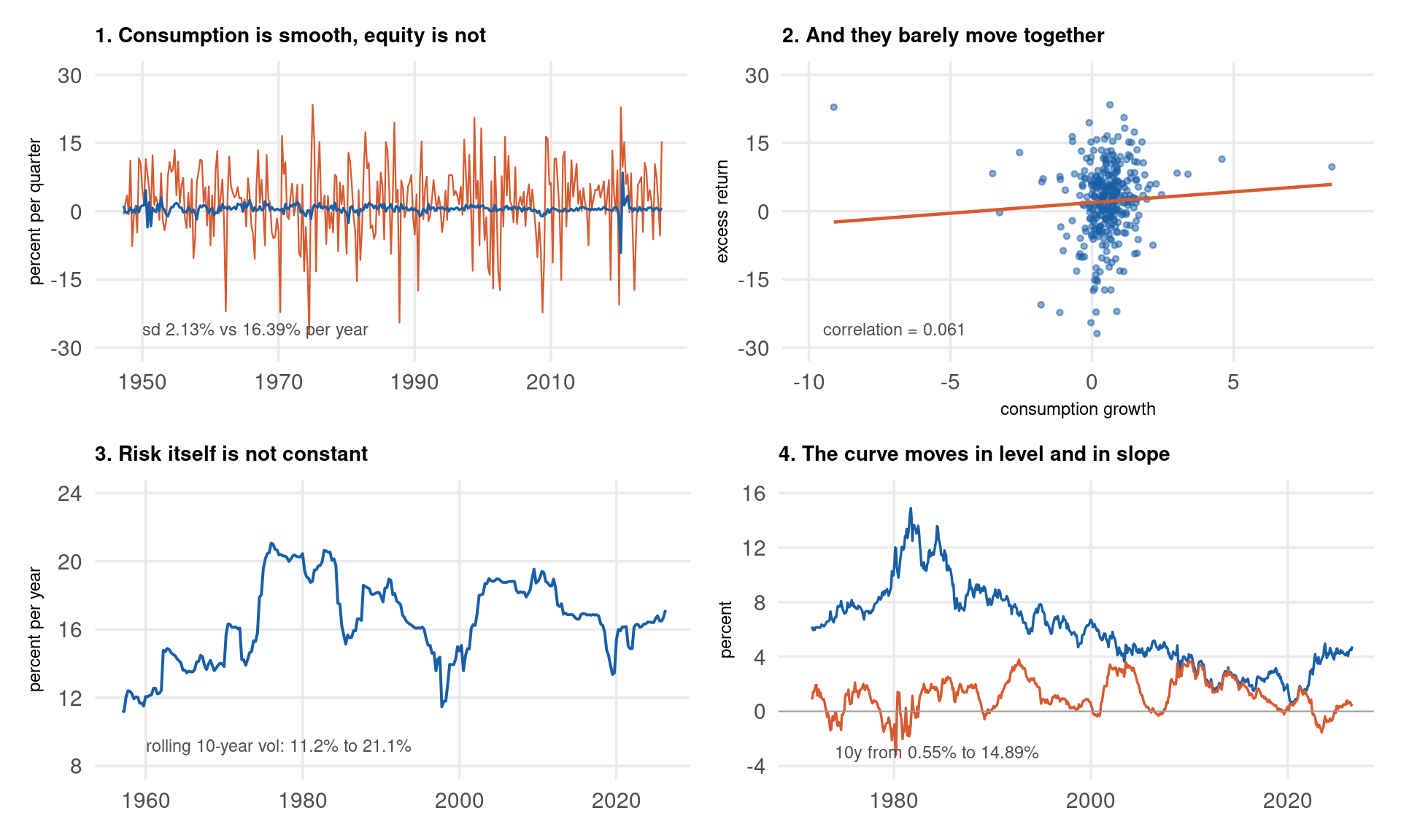
The four facts the rest of the deck is built to confront. Each panel carries the number that makes it a fact rather than an impression.
quietly import delimited "../data/mfsim-equity.csv", clear stringcols(2)generate qtr = substr(date,1,4) + "Q" + string(int((real(substr(date,6,2))-1)/3) + 1, "%1.0f")generate lm = ln(1 + (mktrf + rf)/100)generate lf = ln(1 + rf/100)collapse (sum) lm lf, by(qtr)generate re = 100*(exp(lm) - exp(lf))tempfileeqquietlysave`eq'quietly import delimited "../data/mfsim-macro.csv", clear stringcols(3)keep qtr year dconsquietlymerge 1:1 qtr using`eq', keep(match) nogenerategenerate dc = dcons/4sortyear* Rolling ten-year volatility of the excess return, annualisedgenerate rvol = .forvalues i = 40/`=_N' {quietlysummarize re in`=`i'-39'/`i'quietlyreplace rvol = 2*r(sd) in`i'}twoway (line re year, lcolor("216 90 48") lwidth(vthin)) /// (line dc year, lcolor("24 95 165") lwidth(thin)), ///xscale(range(1947 2026)) yscale(range(-30 30)) ///xlabel(1950(20)2020) ylabel(-30(15)30) ///xtitle("") ytitle("percent per quarter") ///title("1. Consumption is smooth, equity is not", size(medsmall)) ///text(-26 1950 "sd 2.13% vs 16.39% per year", color(gs6) size(vsmall) /// placement(e) justification(left)) ///legend(off) graphregion(color(white)) name(pA, replace)twoway (scatter re dc, mcolor("24 95 165%50") msize(vsmall)) /// (lfit re dc, lcolor("216 90 48") lwidth(medthin)), ///xscale(range(-10 9)) yscale(range(-30 30)) ///xlabel(-10(5)5) ylabel(-30(15)30) ///xtitle("consumption growth") ytitle("excess return") ///title("2. And they barely move together", size(medsmall)) ///text(-26 -9.5 "correlation = 0.061", color(gs6) size(vsmall) /// placement(e) justification(left)) ///legend(off) graphregion(color(white)) name(pB, replace)twoway (line rvol year, lcolor("24 95 165") lwidth(medthin)), ///xscale(range(1957 2026)) yscale(range(8 24)) ///xlabel(1960(20)2020) ylabel(8(4)24) ///xtitle("") ytitle("percent per year") ///title("3. Risk itself is not constant", size(medsmall)) ///text(9.2 1960 "rolling 10-year vol: 11.2% to 21.1%", color(gs6) ///size(vsmall) placement(e) justification(left)) ///legend(off) graphregion(color(white)) name(pC, replace)quietly import delimited "../data/mfsim-yields.csv", clear stringcols(2 3)generate slope = y10 - y01twoway (line y10 year, lcolor("24 95 165") lwidth(thin)) /// (line slope year, lcolor("216 90 48") lwidth(thin)) /// (functiony = 0, range(1971 2026) lcolor(gs10) lwidth(vthin)), ///xscale(range(1971 2026)) yscale(range(-4 16)) ///xlabel(1980(20)2020) ylabel(-4(4)16) ///xtitle("") ytitle("percent") ///title("4. The curve moves in level and in slope", size(medsmall)) ///text(-3 1974 "10y from 0.55% to 14.89%", color(gs6) size(vsmall) /// placement(e) justification(left)) ///legend(off) graphregion(color(white)) name(pD, replace)graphcombine pA pB pC pD, cols(2) graphregion(color(white)) ysize(6) xsize(10)graphexport"../plots/mfsim-facts-stata.png", replacewidth(1900)
Facts 1 and 2 are the puzzle: the asset is volatile, the risk measure is not, and they barely co-move. Fact 3 says a model with constant risk cannot be right — Parts 2 and 6. Fact 4 says the same about a single interest rate — Part 5.
DGP — Mathematical Specification
Five laboratories. Each is simulated once by mfsim-data.R with the seed 14159, and each carries its true parameters as columns in its CSV, so every estimator later in the deck can be scored rather than admired.
I.i.d. lognormal endowment growth with CRRA preferences — the one case where every asset-pricing quantity is closed form, so simulation error can be measured against an exact answer.
\(x_t\) and \(\sigma_t\) are latent — the CSV carries them as x_true and sigma_true so Part 7 can ask whether SMM finds a state nobody observes.
Log-linear real business cycle with fixed labour and log utility. States are capital \(k_t\) and technology \(a_t\); consumption is the forward-looking variable.
Implied: \(g_k = 0.6182\), \(g_a = 0.3052\), \(A_k = 0.9653\). Part 4 solves this same model from scratch with a generalized Schur decomposition and has to land on these three numbers.
The credit spread is a reduced-form accelerator overlay, not a micro-founded contract, and the deck says so rather than dressing it up:
Two affine short-rate models, both simulated by their exact transition laws rather than an Euler step — so Part 2 can measure discretisation bias against a path that has none.
Feller for CIR: \(2(0.35)(0.045) = 0.0315 > 0.0036 = \sigma^2\). Vasicek has no such guarantee and does go negative in this sample — a difference Part 5 uses.
Two states with different means and different variances — the minimum model in which risk is itself a state variable.
The realised path visits state 2 for 12.8% of the sample — close to the share of postwar quarters the NBER dates as recessions. state_true is carried so the three filters in Part 6 are scored on the same answer.
The parity rule. Random-number streams differ across R, Python and Stata, so the same seed does not give the same draws. Every path above is therefore generated once, in mfsim-data.R, and written to a CSV that all three languages read. Where a slide simulates live inside a tab, its numbers will differ in the low-order digits between languages, and the slide says so. The next slide demonstrates exactly that.
DGP — Code Implementation
The Lucas tree, generated live in each language from the parameters on the previous slide. The other four laboratories are generated the same way by mfsim-data.R; only this one is short enough to run on a slide.
Watch the two blocks of output. The closed-form quantities are functions of the parameters alone and agree to every digit printed. The simulated moments come from each language’s own random-number generator and do not.
closed form (parameters only -- identical in every language)
  price-dividend ratio         68.098503
  risk-free rate, % per yr      7.975134
  premium, % per yr             0.036000

simulated (own draws -- differs across languages)
  sd(dc)                        0.007562
  sd(dd)                        0.030416
  E[M R]                        1.000326
Code
import numpy as nprng = np.random.default_rng(14159)n =3000beta, gamma =0.99, 2mu_c, sig_c =0.005, 0.0075mu_d, sig_d, rho =0.005, 0.03, 0.20z1 = rng.normal(size=n)z2 = rng.normal(size=n)dc = mu_c + sig_c * z1dd = mu_d + sig_d * (rho * z1 + np.sqrt(1- rho**2) * z2)# Closed form: a constant price-dividend ratio and a constant risk-free ratek = beta * np.exp(-gamma * mu_c + mu_d+0.5* (gamma**2* sig_c**2+ sig_d**2)- gamma * rho * sig_c * sig_d)pd_ = k / (1- k)rf =1/ (beta * np.exp(-gamma * mu_c +0.5* gamma**2* sig_c**2))sdf = beta * np.exp(-gamma * dc)ret = (1+ pd_) / pd_ * np.exp(dd)out = ("closed form (parameters only -- identical in every language)\n"f" price-dividend ratio {pd_:12.6f}\n"f" risk-free rate, % per yr {400*np.log(rf):12.6f}\n"f" premium, % per yr {400*gamma*rho*sig_c*sig_d:12.6f}\n""\nsimulated (own draws -- differs across languages)\n"f" sd(dc) {dc.std(ddof=1):12.6f}\n"f" sd(dd) {dd.std(ddof=1):12.6f}\n"f" E[M R] {(sdf*ret).mean():12.6f}")import sys; nchars = sys.stdout.write(out +"\n"); sys.stdout.flush()
closed form (parameters only -- identical in every language)
  price-dividend ratio         68.098503
  risk-free rate, % per yr      7.975134
  premium, % per yr             0.036000

simulated (own draws -- differs across languages)
  sd(dc)                        0.007319
  sd(dd)                        0.030084
  E[M R]                        1.000024
Code
* The whole build is silent: only the two blocks at the endprintquietly {clearsetseed 14159setobs 3000scalar beta = 0.99scalargamma = 2scalar mu_c = 0.005scalar sig_c = 0.0075scalar mu_d = 0.005scalar sig_d = 0.03scalar rho = 0.20generatedouble z1 = rnormal()generatedouble z2 = rnormal()generatedouble dc = mu_c + sig_c*z1generatedouble dd = mu_d + sig_d*(rho*z1 + sqrt(1 - rho^2)*z2) * Closed form: a constant price-dividend ratio and a constant risk-free ratescalark = beta*exp(-gamma*mu_c + mu_d /// + 0.5*(gamma^2*sig_c^2 + sig_d^2) - gamma*rho*sig_c*sig_d)scalar pd = k/(1 - k)scalar rf = 1/(beta*exp(-gamma*mu_c + 0.5*gamma^2*sig_c^2))generatedouble sdf = beta*exp(-gamma*dc)generatedouble ret = (1 + pd)/pd*exp(dd)generatedouble mr = sdf*retsummarize dcscalar sdc = r(sd)summarize ddscalar sdd = r(sd)summarize mrscalar emr = r(mean)}display"closed form (parameters only -- identical in every language)"_newline///" price-dividend ratio " %12.6f pd _newline///" risk-free rate, % per yr " %12.6f 400*ln(rf) _newline///" premium, % per yr " %12.6f 400*gamma*rho*sig_c*sig_d _newline///_newline///"simulated (own draws -- differs across languages)"_newline///" sd(dc) " %12.6f sdc _newline///" sd(dd) " %12.6f sdd _newline///" E[M R] " %12.6f emr
closed form (parameters only -- identical in every language)
  price-dividend ratio         68.098503
  risk-free rate, % per yr      7.975134
  premium, % per yr             0.036000

simulated (own draws -- differs across languages)
  sd(dc)                        0.007460
  sd(dd)                        0.029889
  E[M R]                        1.000122
DGP — Diagnostics
reference depth — scrollable, read after class
Now the opposite test. Every tab below reads the same CSVs, so every number must agree to the last printed digit in all three languages. Each row scores a laboratory against the truth columns it carries.
Code
lu <-read.csv("../data/mfsim-lucas.csv")lr <-read.csv("../data/mfsim-lrr.csv")ds <-read.csv("../data/mfsim-dsge.csv")tm <-read.csv("../data/mfsim-term.csv")rg <-read.csv("../data/mfsim-regime.csv")ac1 <-function(x) cor(x[-1], x[-length(x)])# The RBC policy rule is deterministic, so OLS must return it exactlynd <-nrow(ds)fit <-lm(ds$k[-1] ~ ds$k[-nd] + ds$a[-nd])# Transition probabilities from the realised regime pathnr <-nrow(rg)s0 <- rg$state_true[-nr]; s1 <- rg$state_true[-1]p11 <-sum(s0 ==1& s1 ==1) /sum(s0 ==1)p22 <-sum(s0 ==2& s1 ==2) /sum(s0 ==2)
    Lab     Diagnostic Recovered    Truth       Gap
  lucas         E[M R]  1.000326 1.000000  0.000326
  lucas         sd(dc)  0.007562 0.007500  0.000062
    lrr         ac1(x)  0.977298 0.979000 -0.001702
    lrr   ac1(sigma^2)  0.977554 0.987000 -0.009446
    rbc     A_k by OLS  0.965276 0.965276  0.000000
    rbc     B_a by OLS  0.075372 0.075372  0.000000
   term ac1(r Vasicek)  0.976910 0.975310  0.001600
   term    mean(r CIR)  0.041399 0.045000 -0.003601
   term     min(r CIR)  0.011946 0.000000  0.011946
 regime            p11  0.968481 0.950000  0.018481
 regime            p22  0.792079 0.750000  0.042079
policy rule check: max |c - (g_k k + g_a a)| = 1.07e-14
(1 missing value generated)


(1 missing value generated)


(1 missing value generated)

(1 missing value generated)


(1 missing value generated)


(1 missing value generated)

    Lab      Diagnostic    Recovered        Truth          Gap


  5. }
  lucas          E[M R]     1.000326     1.000000     0.000326
  lucas          sd(dc)     0.007562     0.007500     0.000062
    lrr          ac1(x)     0.977298     0.979000    -0.001702
    lrr    ac1(sigma^2)     0.977554     0.987000    -0.009446
    rbc      A_k by OLS     0.965276     0.965276     0.000000
    rbc      B_a by OLS     0.075372     0.075372    -0.000000
   term  ac1(r Vasicek)     0.976910     0.975310     0.001600
   term     mean(r CIR)     0.041399     0.045000    -0.003601
   term      min(r CIR)     0.011946     0.000000     0.011946
 regime             p11     0.968481     0.950000     0.018481
 regime             p22     0.792079     0.750000     0.042079


policy rule check: max |c - (g_k k + g_a a)| =  1.1e-14
How to read the gaps
Two rows are exact — A_k and B_a come back to six decimals with \(R^2 = 1\), because the RBC policy rule is deterministic and OLS is simply inverting it.
Every other row carries sampling error, and the persistent ones carry the most: ac1(sigma^2) lands at 0.978 against a true 0.987, because the AR(1) coefficient of a near-unit-root process is biased downward in finite samples by roughly
\[\text{bias} \;\approx\; \frac{1 + 3\nu}{T}\]
That bias is a fact about the estimator, not a flaw in the data — and Part 7 returns to it when a century of observations turns out not to be many.
Part 2 — The Simulation Toolkit
Discretising persistent processes, simulating stochastic differential equations, Monte Carlo error, and variance reduction.
Almost every model in this deck contains a continuous state that follows an AR(1): technology in the RBC model, the long-run risk component \(x_t\), the short rate. To solve such a model on a computer you usually have to replace that continuous state with a finite Markov chain — a handful of grid points and a transition matrix.
The obvious question is how many points you need. The more interesting question, and the one that decides whether Part 3 works at all, is which method.
The long-run risk calibration has \(\rho = 0.979\). That is exactly where the textbook method stops working — and where the method almost nobody teaches first is still exact.
Two candidates:
Tauchen (1986) — put evenly spaced points on the grid, then integrate the normal density over the cell around each one. Intuitive, and the standard choice.
Rouwenhorst — forget the density; build the chain recursively from a two-state binomial so that its mean, variance and autocorrelation match the AR(1) by construction, for any \(N\) and any \(\rho\).
Tauchen. Place \(N\) evenly spaced points on \([-m\sigma_z,\; m\sigma_z]\) with spacing \(w\), then assign each cell the normal probability of landing in it:
halving every interior row so each sums to one. The grid spans
\[\pm \, \psi = \pm \, \sigma_z \sqrt{N-1}\]
and it is a theorem, not an approximation, that the resulting chain reproduces \(\rho\) and \(\sigma_z\) exactly.
Tauchen & Rouwenhorst — Code
Both methods are deterministic functions of \((N, \rho, \sigma)\), so all three languages must return the same transition matrix. Here \(N = 9\), \(\rho = 0.9\), \(\sigma = 0.01\).
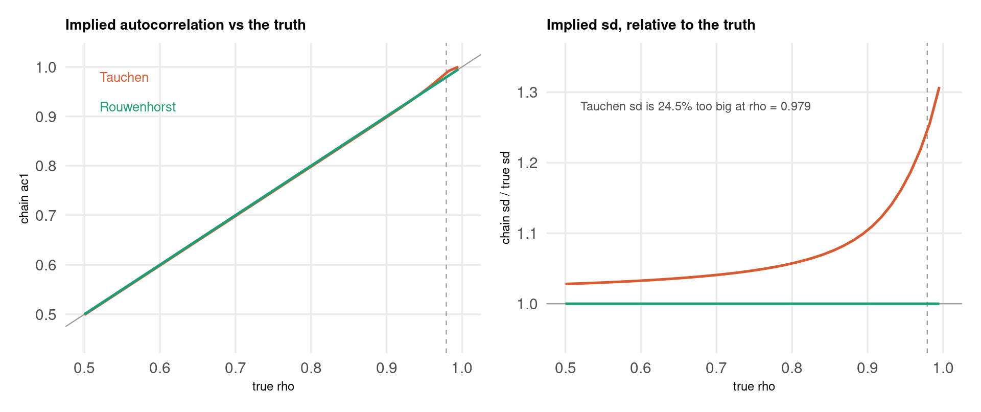
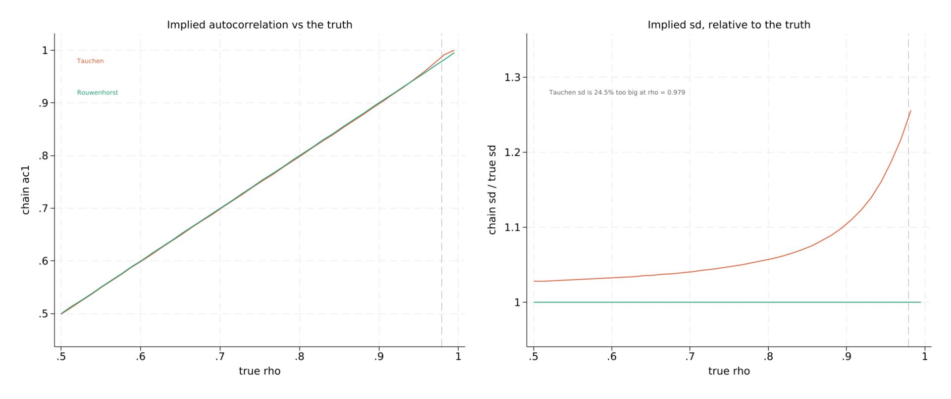
For each \(\rho\), build a 9-state chain, compute its stationary standard deviation and first autocorrelation, and compare them with the AR(1) they are supposed to represent. The dashed line marks \(\rho = 0.979\) — the long-run risk calibration from Part 1.
Code
# Stationary distribution: the left eigenvector of P with eigenvalue 1stat_dist <-function(P) { e <-eigen(t(P)) v <-Re(e$vectors[, which.max(Re(e$values))]) v /sum(v)}# Implied sd and first autocorrelation of a finite chainchain_moments <-function(g) { pr <-stat_dist(g$P) m <-sum(pr * g$z) v <-sum(pr * (g$z - m)^2) ez <-0for (i inseq_along(g$z)) ez <- ez + pr[i] * g$z[i] *sum(g$P[i, ] * g$z)c(sd =sqrt(v), ac1 = (ez - m^2) / v)}rhos <-seq(0.50, 0.995, length.out =40)acc <-data.frame(rho = rhos, t_ac1 =NA, r_ac1 =NA, t_sd =NA, r_sd =NA)for (i inseq_along(rhos)) { mt <-chain_moments(tauchen(9, rhos[i], 0.01)) mr <-chain_moments(rouwenhorst(9, rhos[i], 0.01)) true_sd <-0.01/sqrt(1- rhos[i]^2) acc[i, 2:5] <-c(mt["ac1"], mr["ac1"], mt["sd"] / true_sd, mr["sd"] / true_sd)}
Code
import matplotlib.pyplot as pltdef stat_dist(P): w, v = np.linalg.eig(P.T) x = np.real(v[:, np.argmax(np.real(w))])return x / x.sum()def chain_moments(z, P): pr = stat_dist(P) m = (pr * z).sum() v = (pr * (z - m)**2).sum() ez =sum(pr[i] * z[i] * (P[i, :] * z).sum() for i inrange(len(z)))return np.sqrt(v), (ez - m**2) / vrhos = np.linspace(0.50, 0.995, 40)t_ac1, r_ac1, t_sd, r_sd = [], [], [], []for r in rhos: zt, Pt = tauchen(9, r, 0.01) zr, Pr = rouwenhorst(9, r, 0.01) st, at = chain_moments(zt, Pt) sr, ar = chain_moments(zr, Pr) true_sd =0.01/ np.sqrt(1- r**2) t_ac1.append(at); r_ac1.append(ar) t_sd.append(st / true_sd); r_sd.append(sr / true_sd)fig, ax = plt.subplots(1, 2, figsize=(10, 4.2))ax[0].plot([0.5, 1.0], [0.5, 1.0], color="#999999", lw=0.7)ax[0].axvline(0.979, color="#999999", ls="--", lw=0.7)ax[0].plot(rhos, t_ac1, color="#D85A30", lw=1.5)ax[0].plot(rhos, r_ac1, color="#1D9E75", lw=1.5)ax[0].text(0.52, 0.98, "Tauchen", color="#D85A30", fontsize=9)ax[0].text(0.52, 0.92, "Rouwenhorst", color="#1D9E75", fontsize=9)a1 = ax[0].set(xlim=(0.50, 1.00), ylim=(0.45, 1.02), xticks=np.arange(0.5, 1.01, 0.1), yticks=np.arange(0.5, 1.01, 0.1), xlabel="true rho", ylabel="chain ac1", title="Implied autocorrelation vs the truth")ax[1].axhline(1, color="#999999", lw=0.7)ax[1].axvline(0.979, color="#999999", ls="--", lw=0.7)ax[1].plot(rhos, t_sd, color="#D85A30", lw=1.5)ax[1].plot(rhos, r_sd, color="#1D9E75", lw=1.5)ax[1].text(0.52, 1.28, "Tauchen sd is 24.5% too big at rho = 0.979", color="#4d4d4d", fontsize=8)a2 = ax[1].set(xlim=(0.50, 1.00), ylim=(0.95, 1.35), xticks=np.arange(0.5, 1.01, 0.1), yticks=np.arange(1.0, 1.36, 0.1), xlabel="true rho", ylabel="chain sd / true sd", title="Implied sd, relative to the truth")fig.tight_layout()plt.show()
Rouwenhorst is exact everywhere; Tauchen is not. The green lines sit on the truth at every persistence, because matching \(\rho\) and \(\sigma_z\) is built into the construction rather than approximated. Tauchen’s chain is 10% too volatile at \(\rho = 0.9\), 24.5% too volatile at \(\rho = 0.979\), and its autocorrelation overshoots to 0.9999 by \(\rho = 0.995\): a fixed grid of nine points spanning \(\pm 3\sigma_z\) simply cannot represent a process that spends most of its time far from the mean. Use Rouwenhorst for anything persistent, which in macro-finance is nearly everything.
Asset-pricing models are written in continuous time; computers work in discrete steps. Bridging that gap is a modelling decision, not a technicality, and it has three answers.
Exact simulation. For a few processes the transition law is known in closed form, so you can jump from \(t\) to \(t+\Delta\) with no error at all, however large the step. The Vasicek and CIR paths in Part 1 were built this way.
Euler–Maruyama. Replace \(dW\) with \(\sqrt{\Delta}\,z\). Always available, always biased.
Milstein. Add the term in the derivative of the diffusion coefficient. It buys nothing when the diffusion is constant, and helps when it is not.
Euler’s error is not only a matter of accuracy. Applied to CIR it puts positive probability on a negative interest rate — a state the true process can never reach. Some errors shrink with \(\Delta\); some break the model.
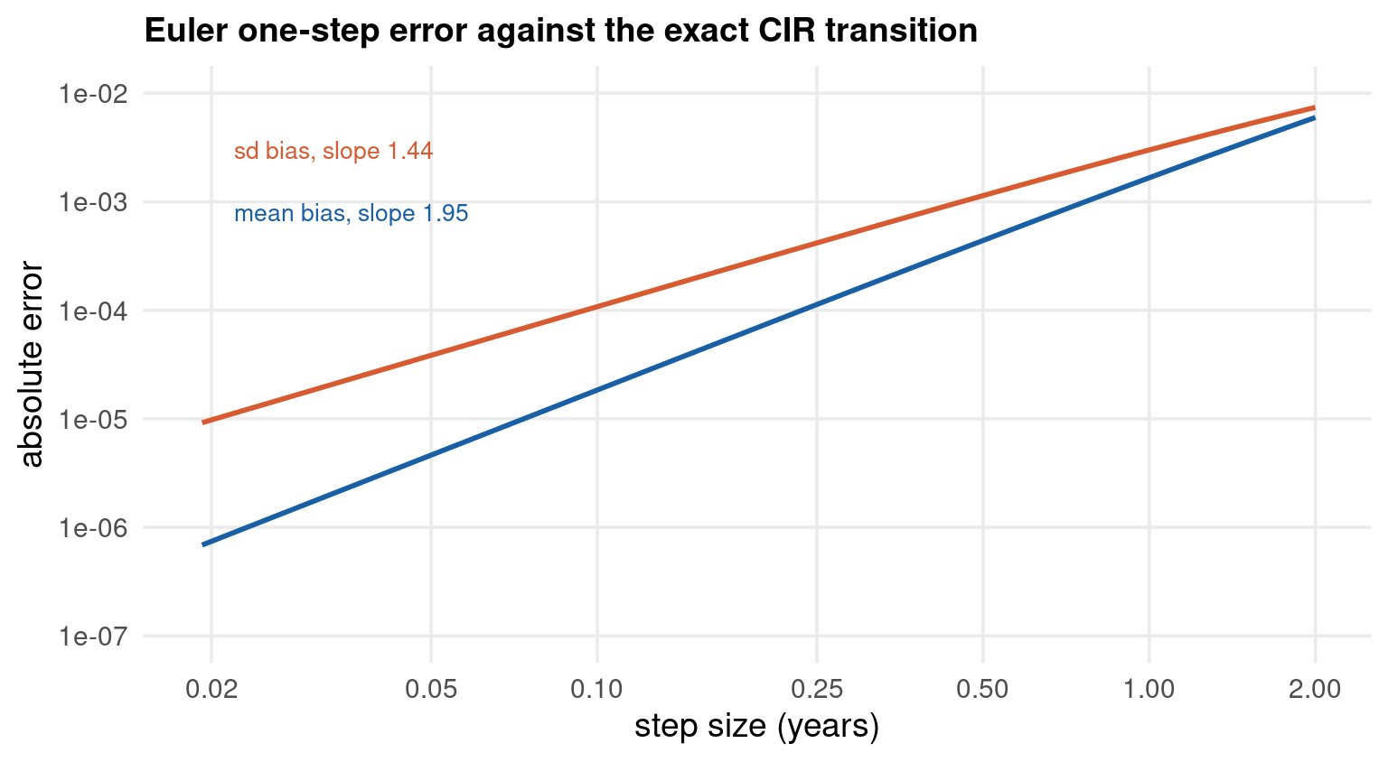
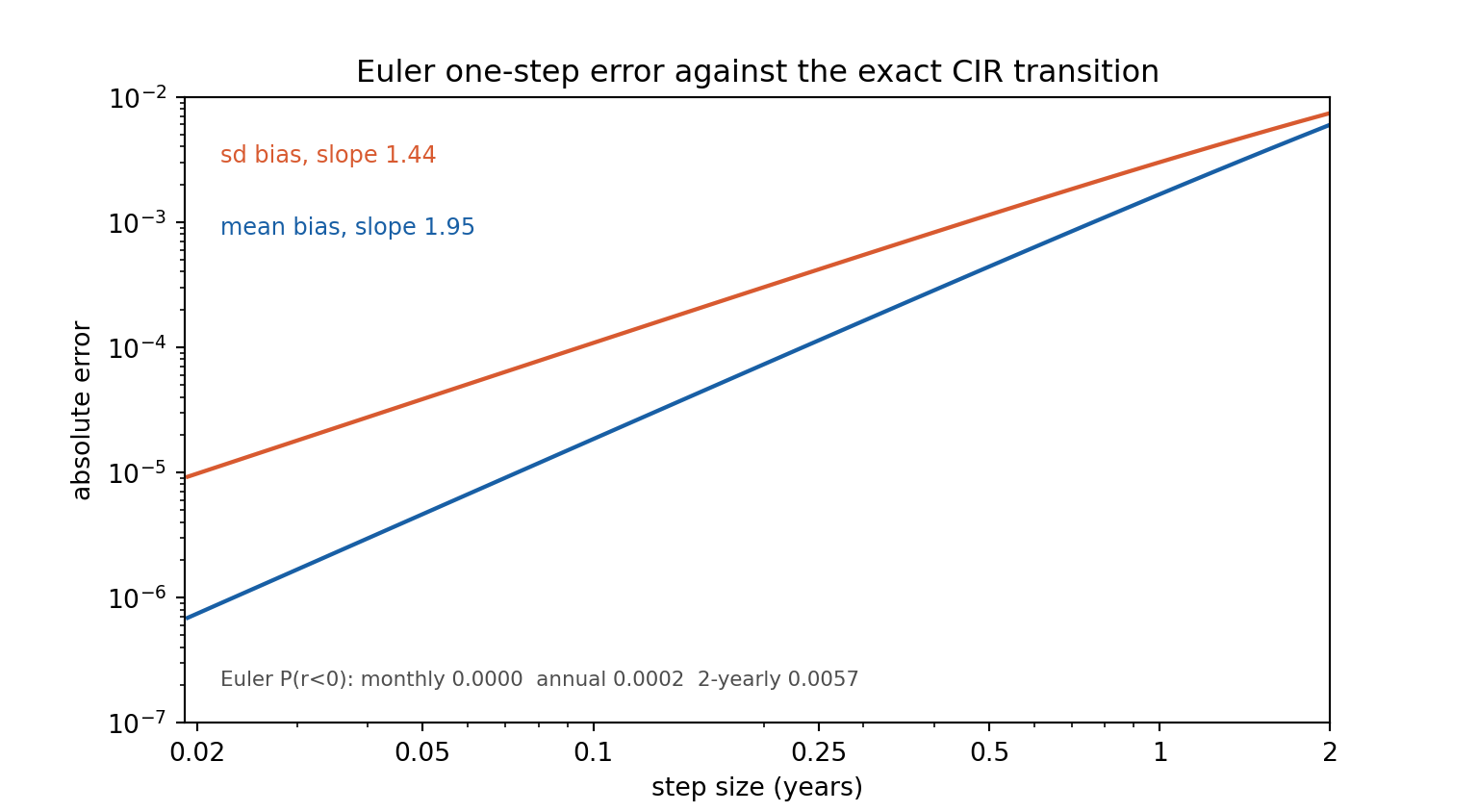
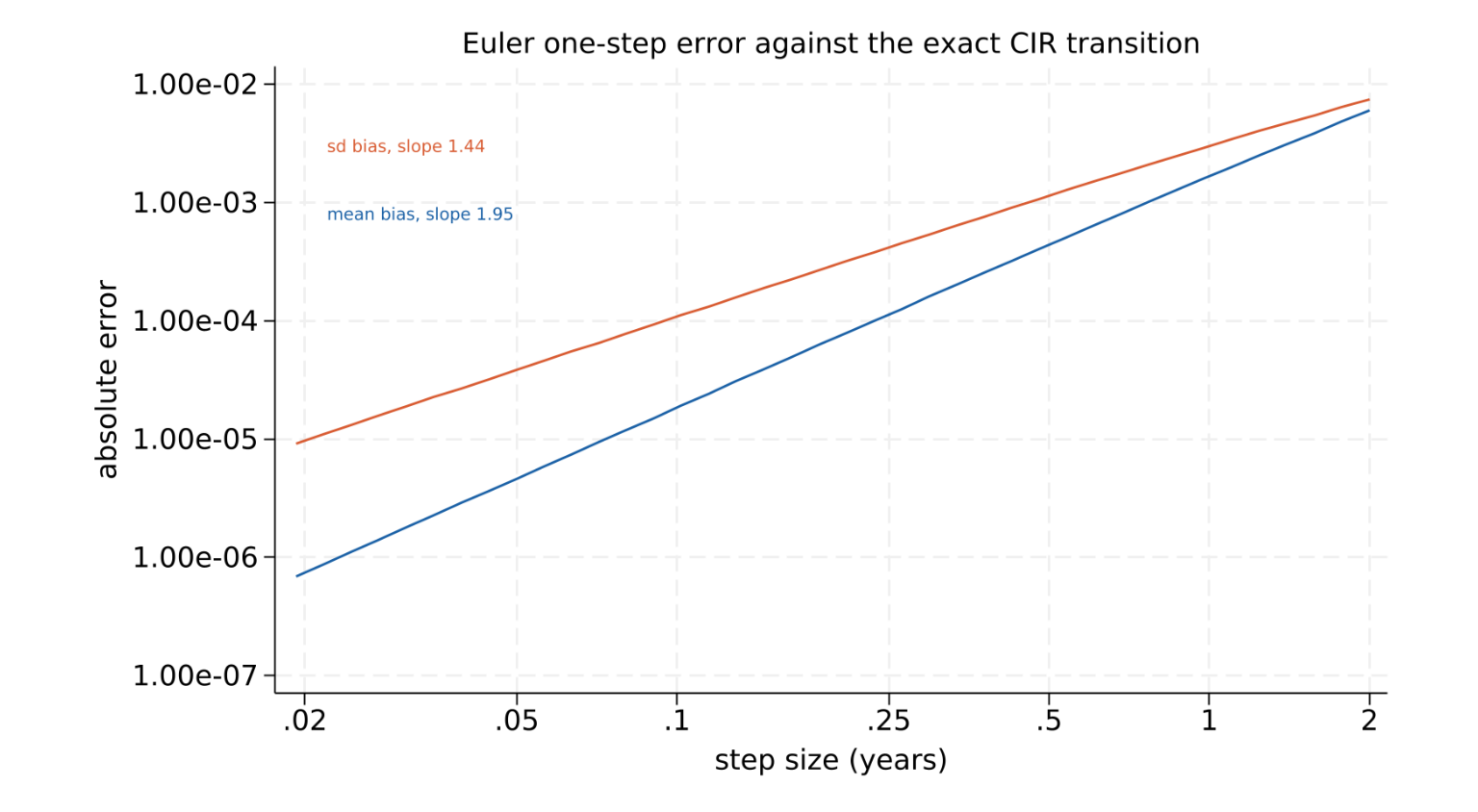
Euler’s conditional moments are \(r_t + \kappa(\theta - r_t)\Delta\) and \(\sigma^2 r_t \Delta\). Expanding the exponentials gives the local, one-step error orders:
\[\left| \text{bias in mean} \right| = O(\Delta^2), \qquad \left| \text{bias in sd} \right| = O(\Delta^{3/2})\]
which accumulate over \(T/\Delta\) steps to the familiar global weak order one.
Discretisation Bias — Code & Plot
The two curves are the analytic one-step errors of the Euler scheme against the exact CIR transition, evaluated at \(r_t = \theta + 2\sigma_{\text{stat}}\). They contain no simulation at all, so all three languages trace the same lines. Printed underneath is the one thing only simulation can show: how often Euler sends the rate below zero.
Code
kap <-0.35; th <-0.045; sig <-0.06sd_stat <-sqrt(sig^2* th / (2* kap))rt <- th +2* sd_statdts <-exp(seq(log(1/52), log(2), length.out =40))bias <-data.frame(dt = dts) |>mutate(mean_bias =abs((rt - th) * (exp(-kap * dt) - (1- kap * dt))),var_exact = rt * sig^2* (exp(-kap*dt) -exp(-2*kap*dt)) / kap + th * sig^2* (1-exp(-kap*dt))^2/ (2*kap),sd_bias =abs(sqrt(var_exact) -sqrt(sig^2* rt * dt)))# How often does Euler leave the state space the true process never leaves?set.seed(14159)n <-200000euler_neg <-function(dt) { e <-numeric(n); e[1] <- th z <-rnorm(n)for (i in2:n) { rp <-max(e[i-1], 0) e[i] <- e[i-1] + kap * (th - rp) * dt + sig *sqrt(rp * dt) * z[i] }mean(e <0)}
Feller condition 2*kappa*theta > sigma^2:  0.0315 > 0.0036  -- the exact process never goes negative

Euler P(r < 0):  monthly 0.0000   annual 0.0002   two-yearly 0.0057
Code
import numpy as npimport matplotlib.pyplot as pltkap, th, sig =0.35, 0.045, 0.06sd_stat = np.sqrt(sig**2* th / (2* kap))rt = th +2* sd_statdts = np.exp(np.linspace(np.log(1/52), np.log(2), 40))mean_bias = np.abs((rt - th) * (np.exp(-kap*dts) - (1- kap*dts)))var_exact = (rt * sig**2* (np.exp(-kap*dts) - np.exp(-2*kap*dts)) / kap+ th * sig**2* (1- np.exp(-kap*dts))**2/ (2*kap))sd_bias = np.abs(np.sqrt(var_exact) - np.sqrt(sig**2* rt * dts))sm = np.log(mean_bias[-1]/mean_bias[0]) / np.log(dts[-1]/dts[0])ss = np.log(sd_bias[-1]/sd_bias[0]) / np.log(dts[-1]/dts[0])# How often does Euler leave the state space the true process never leaves?rng = np.random.default_rng(14159)n =200000def euler_neg(dt): e = np.empty(n); e[0] = th z = rng.normal(size=n)for i inrange(1, n): rp =max(e[i-1], 0.0) e[i] = e[i-1] + kap*(th - rp)*dt + sig*np.sqrt(rp*dt)*z[i]return (e <0).mean()pn = [euler_neg(1/12), euler_neg(1.0), euler_neg(2.0)]fig, ax = plt.subplots(figsize=(8, 4.4))ax.plot(dts, mean_bias, color="#185FA5", lw=1.6)ax.plot(dts, sd_bias, color="#D85A30", lw=1.6)ax.text(0.022, 3e-3, f"sd bias, slope {ss:.2f}", color="#D85A30", fontsize=9)ax.text(0.022, 8e-4, f"mean bias, slope {sm:.2f}", color="#185FA5", fontsize=9)ax.text(0.022, 2e-7,f"Euler P(r<0): monthly {pn[0]:.4f} annual {pn[1]:.4f} 2-yearly {pn[2]:.4f}", color="#4d4d4d", fontsize=8)axopts = ax.set(xscale="log", yscale="log", xlim=(0.019, 2), ylim=(1e-7, 1e-2), xlabel="step size (years)", ylabel="absolute error", title="Euler one-step error against the exact CIR transition")ax.set_xticks([0.02, 0.05, 0.1, 0.25, 0.5, 1, 2])ax.set_xticklabels(["0.02","0.05","0.1","0.25","0.5","1","2"])plt.show()
A simulated answer is an estimate, and it comes with a standard error you are obliged to report. Three practical consequences run through the rest of the deck.
The \(1/\sqrt{B}\) wall. Halving the Monte Carlo error costs four times the paths. Beyond a point, buying accuracy with raw draws stops being sensible and you change the estimator instead.
Burn-in. A simulation started away from the ergodic distribution carries its initial condition for a while. Every simulated laboratory in this deck discards a burn-in — 500 to 600 draws — and the DGP script says how many.
Variance reduction. Three cheap tricks routinely buy what a hundredfold increase in paths would: exploit symmetry, exploit something whose answer you already know, or stop drawing at random altogether.
For an estimator \(\hat\mu_B\) built from \(B\) independent draws:
Quasi-Monte Carlo. Replace pseudo-random draws by a low-discrepancy (Sobol) net. The error becomes \(O\!\left( (\log B)^d / B \right)\) rather than \(O(B^{-1/2})\); a random shift restores an honest variance estimate.
Each method uses 2000 paths, repeated 50 times, so the spread across runs is the estimator’s own standard error.
Code
kap <-0.30; th <-0.045; sig <-0.015; r0 <-0.045Tm <-5; m <-60; dt <- Tm / me1 <-exp(-kap * dt)s1 <- sig *sqrt((1-exp(-2* kap * dt)) / (2* kap))B <- (1-exp(-kap * Tm)) / kapAa <- (B - Tm) * (kap^2* th - sig^2/2) / kap^2- sig^2* B^2/ (4* kap)truth <-exp(Aa - B * r0)Eint <- th * Tm + (r0 - th) * (1-exp(-kap * Tm)) / kap# One vectorised sweep: every path advances together, step by stepsim_int <-function(Z) { r <-rep(r0, nrow(Z)); s <-rep(0, nrow(Z))for (k in1:ncol(Z)) { r <- th + (r - th) * e1 + s1 * Z[, k] s <- s + r * dt } s}set.seed(14159)M <-2000; R <-50Us <-sobol(M, m) # one Sobol net, shifted each runres <-matrix(NA, R, 4)for (rep in1:R) { Z <-matrix(rnorm(M * m), M, m) I <-sim_int(Z); y <-exp(-I) res[rep, 1] <-mean(y) # plain h <- M /2; Zh <- Z[1:h, , drop =FALSE] res[rep, 2] <-mean(c(exp(-sim_int(Zh)), exp(-sim_int(-Zh)))) # antithetic b <-cov(y, I) /var(I) res[rep, 3] <-mean(y - b * (I - Eint)) # control variate sh <-matrix(runif(m), M, m, byrow =TRUE) # random shift Zq <-qnorm(pmin(pmax((Us + sh) %%1, 1e-12), 1-1e-12)) res[rep, 4] <-mean(exp(-sim_int(Zq))) # quasi-Monte Carlo}
closed-form P(0,5) = 0.79991940     M = 2000 paths, R = 50 runs

          Method        Bias          SE   VarRatio
        plain MC    1.90e-05    1.10e-03        1.0
      antithetic    3.21e-05    6.57e-05      280.9
 control variate    2.22e-05    5.26e-05      438.1
       Sobol QMC    1.01e-05    9.73e-05      128.2
Code
import numpy as npfrom scipy.stats import qmc, normkap, th, sig, r0 =0.30, 0.045, 0.015, 0.045Tm, m =5, 60dt = Tm / me1 = np.exp(-kap * dt)s1 = sig * np.sqrt((1- np.exp(-2* kap * dt)) / (2* kap))Bv = (1- np.exp(-kap * Tm)) / kapAa = (Bv - Tm) * (kap**2* th - sig**2/2) / kap**2- sig**2* Bv**2/ (4*kap)truth = np.exp(Aa - Bv * r0)Eint = th * Tm + (r0 - th) * (1- np.exp(-kap * Tm)) / kap# One vectorised sweep: every path advances together, step by stepdef sim_int(Z): r = np.full(Z.shape[0], r0) s = np.zeros(Z.shape[0])for k inrange(Z.shape[1]): r = th + (r - th) * e1 + s1 * Z[:, k] s = s + r * dtreturn srng = np.random.default_rng(14159)M, R =2000, 50Us = qmc.Sobol(d=m, scramble=False).random(M) # one Sobol net, shifted each runres = np.zeros((R, 4))for rep inrange(R): Z = rng.normal(size=(M, m)) I = sim_int(Z); y = np.exp(-I) res[rep, 0] = y.mean() h = M //2; Zh = Z[:h, :] res[rep, 1] = np.concatenate([np.exp(-sim_int(Zh)), np.exp(-sim_int(-Zh))]).mean() b = np.cov(y, I, ddof=1)[0, 1] / I.var(ddof=1) res[rep, 2] = (y - b * (I - Eint)).mean() sh = rng.random(m) # random shift Zq = norm.ppf(np.clip((Us + sh) %1, 1e-12, 1-1e-12)) res[rep, 3] = np.exp(-sim_int(Zq)).mean()nm = ["plain MC", "antithetic", "control variate", "Sobol QMC"]v1 = res[:, 0].var(ddof=1)lines = [f"closed-form P(0,5) = {truth:.8f} M = 2000 paths, R = 50 runs", "",f"{'Method':>16}{'Bias':>11}{'SE':>11}{'VarRatio':>10}"]for j, nmj inenumerate(nm): lines.append(f"{nmj:>16}{res[:,j].mean()-truth:11.2e} "f"{res[:,j].std(ddof=1):11.2e}{v1/res[:,j].var(ddof=1):10.1f}")import sys; nchars = sys.stdout.write("\n".join(lines) +"\n"); sys.stdout.flush()
closed-form P(0,5) = 0.79991940     M = 2000 paths, R = 50 runs

          Method        Bias          SE   VarRatio
        plain MC    2.47e-04    1.15e-03        1.0
      antithetic    2.44e-05    7.25e-05      253.0
 control variate    2.51e-05    4.56e-05      638.2
       Sobol QMC    1.32e-05    7.50e-05      236.2
Code
quietly {scalarkap = 0.30scalar th = 0.045scalar sig = 0.015scalar r0 = 0.045scalar Tm = 5scalarm = 60scalar dt = Tm/mscalar e1 = exp(-kap*dt)scalar s1 = sig*sqrt((1 - exp(-2*kap*dt))/(2*kap))scalar Bv = (1 - exp(-kap*Tm))/kapscalar Aa = (Bv - Tm)*(kap^2*th - sig^2/2)/kap^2 - sig^2*Bv^2/(4*kap)scalar truth = exp(Aa - Bv*r0)scalar Eint = th*Tm + (r0 - th)*(1 - exp(-kap*Tm))/kapclearsetseed 14159setobs 2000generatedoubley = .generatedouble ya = .generatedouble yc = .generatedouble ii = .tempname pftempfile runspostfile`pf' m1 m2 m3 using`runs'forvalues rep = 1/50 { * plain and antithetic share one setof shocks; the integral is the * control variate, and its mean is known in closed formreplace ii = 0generatedoubler = r0generatedouble ra = r0generatedouble ia = 0forvaluesk = 1/60 {generatedouble z = rnormal()replacer = th + (r - th)*e1 + s1*zreplace ra = th + (ra - th)*e1 - s1*zreplace ii = ii + r*dtreplace ia = ia + ra*dtdrop z }replacey = exp(-ii)replace ya = exp(-ia)summarize ii, meanonlyscalarmi = r(mean) correlate y ii, covariancescalar bb = r(cov_12)/r(Var_2)replace yc = y - bb*(ii - Eint)summarizey, meanonlyscalar s_plain = r(mean)generatedouble ymid = (y + ya)/2summarize ymid, meanonlyscalar s_anti = r(mean)summarize yc, meanonlyscalar s_cv = r(mean)post`pf' (s_plain) (s_anti) (s_cv)dropr ra ia ymid }postclose`pf'use`runs', clearsummarize m1scalar b1 = r(mean) - truthscalar e_1 = r(sd)summarize m2scalar b2 = r(mean) - truthscalar e_2 = r(sd)summarize m3scalar b3 = r(mean) - truthscalar e_3 = r(sd)}display"closed-form P(0,5) = " %10.8f truth ///" M = 2000 paths, R = 50 runs"_newline///_newline///" Method Bias SE VarRatio"_newline///" plain MC " %10.2e b1 " " %10.2e e_1 " " %9.1f 1 _newline///" antithetic " %10.2e b2 " " %10.2e e_2 " " %9.1f (e_1/e_2)^2 _newline///" control variate " %10.2e b3 " " %10.2e e_3 " " %9.1f (e_1/e_3)^2
closed-form P(0,5) = 0.79991940     M = 2000 paths, R = 50 runs

          Method        Bias          SE   VarRatio
        plain MC   -2.44e-05    1.25e-03        1.0
      antithetic    2.59e-05    5.24e-05      573.4
 control variate    2.42e-05    5.30e-05      561.7
Stata has no Sobol generator — neither built in nor on SSC — so the quasi-Monte Carlo row has no Stata counterpart. The other three methods are implemented in full.
All three tricks pay
None of them costs an extra path. Antithetic sampling works here because \(\exp(-\int r)\) is monotone in the shocks, so a draw and its mirror image land on opposite sides of the answer. The control variate does better still, because the integral it corrects with is almost perfectly correlated with the payoff. Quasi-Monte Carlo wins by filling the 60-dimensional cube more evenly than randomness manages. The lesson is the one the \(1/\sqrt{B}\) law forces: past a point, change the estimator, not the number of draws.
Part 3 — Consumption-Based Asset Pricing
The Lucas tree, Epstein-Zin preferences, long-run risk, habit formation, rare disasters, and a horse race against the data.
The simplest complete asset-pricing model there is. One representative consumer, one tree, and the tree’s fruit is aggregate consumption — so there is nothing to save and nothing to invest. In equilibrium the consumer eats the endowment and prices adjust until she is content to do so.
That sounds too simple to be interesting. It is exactly the point: with i.i.d. lognormal growth and CRRA preferences every quantity is closed form, so when the model fails we know it is the economics failing, not the numerics.
Where this model sits in the literature
This is the model Mehra and Prescott put to the data in 1985. Everything in the rest of Part 3 — recursive utility, long-run risk, habit, disasters — is an attempt to repair what the next two slides break.
Three small numbers multiplied together, scaled by \(\gamma\). Nothing else is available to make it large.
value
source
\(\beta\)
0.99 per quarter
conventional; implies a 4% annual discount rate
\(\gamma\)
2
the range experimental evidence supports
\(\mu_c\)
0.005
2% per year, matching the 2.08% measured in Part 1
\(\sigma_c\)
0.0075
1.5% per year, the smoother pre-COVID reading
\(\mu_d\)
0.005
dividends grow with consumption
\(\sigma_d\)
0.03
6% per year — dividends are four times more volatile
\(\rho\)
0.20
generous: the measured value in Part 1 is 0.061
Every one of these is chosen to give the model its best shot. The correlation in particular is set more than three times the value in the data.
Lucas Tree — Code: Simulate and Price
Reading ../data/mfsim-lucas.csv, written once by mfsim-data.R — so all three tabs price the identical 3000-quarter path.
Code
lu <-read.csv("../data/mfsim-lucas.csv")# Everything below is already implied by the parameters; the simulated path is# used only to confirm the closed forms and to show the Euler equation holds.beta <- lu$beta_true[1]; gamma <- lu$gamma_true[1]pd <- lu$pd[1]rf <- lu$rf[1]ER <-mean(lu$ret)prem <- ER - rfeuler <-mean(lu$sdf * lu$ret)# The same premium from the covariance formula, as a cross-checkprem_cov <--cov(lu$sdf, lu$ret) /mean(lu$sdf)
Lucas tree, 3000 quarters, beta = 0.99, gamma = 2

  price-dividend ratio           68.0985
  risk-free rate                  7.9751 % per year
  E[R]                            8.0838 % per year
  equity premium                  0.0286 % per year
  same, from -cov(M,R)/E[M]       0.0399 % per year

  Euler equation E[M R]        1.000326  (must be 1)
Code
import numpy as npimport pandas as pdlu = pd.read_csv("../data/mfsim-lucas.csv")# Everything below is already implied by the parameters; the simulated path is# used only to confirm the closed forms and to show the Euler equation holds.beta, gamma = lu["beta_true"][0], lu["gamma_true"][0]pd_ = lu["pd"][0]rf = lu["rf"][0]ER = lu["ret"].mean()prem = ER - rfeuler = (lu["sdf"] * lu["ret"]).mean()# The same premium from the covariance formula, as a cross-checkprem_cov =-np.cov(lu["sdf"], lu["ret"], ddof=1)[0, 1] / lu["sdf"].mean()out = (f"Lucas tree, {len(lu)} quarters, beta = {beta:.2f}, gamma = {gamma:.0f}\n\n"f" price-dividend ratio {pd_:10.4f}\n"f" risk-free rate {400*np.log(rf):10.4f} % per year\n"f" E[R] {400*(ER-1):10.4f} % per year\n"f" equity premium {400*prem:10.4f} % per year\n"f" same, from -cov(M,R)/E[M] {400*prem_cov:10.4f} % per year\n"f"\n Euler equation E[M R] {euler:10.6f} (must be 1)\n")import sys; nchars = sys.stdout.write(out); sys.stdout.flush()
Lucas tree, 3000 quarters, beta = 0.99, gamma = 2

  price-dividend ratio           68.0985
  risk-free rate                  7.9751 % per year
  E[R]                            8.0838 % per year
  equity premium                  0.0286 % per year
  same, from -cov(M,R)/E[M]       0.0399 % per year

  Euler equation E[M R]        1.000326  (must be 1)
Code
quietly { import delimited "../data/mfsim-lucas.csv", clearscalar beta = beta_true[1]scalargamma = gamma_true[1]scalar pd = pd[1]scalar rf = rf[1]scalar nq = _Nsummarize ret, meanonlyscalar ER = r(mean)scalar prem = ER - rfgeneratedouble mr = sdf*retsummarize mr, meanonlyscalar euler = r(mean) * The same premium from the covariance formula, as a cross-check correlate sdf ret, covariancescalar cmr = r(cov_12)summarize sdf, meanonlyscalar prem_cov = -cmr/r(mean)}display"Lucas tree, " %4.0f nq " quarters, beta = " %4.2f beta ///", gamma = " %2.0f gamma_newline///_newline///" price-dividend ratio " %10.4f pd _newline///" risk-free rate " %10.4f 400*ln(rf) " % per year"_newline///" E[R] " %10.4f 400*(ER-1) " % per year"_newline///" equity premium " %10.4f 400*prem " % per year"_newline///" same, from -cov(M,R)/E[M] " %10.4f 400*prem_cov " % per year"_newline///_newline///" Euler equation E[M R] " %10.6f euler " (must be 1)"
Lucas tree, 3000 quarters, beta = 0.99, gamma =  2

  price-dividend ratio           68.0985
  risk-free rate                  7.9751 % per year
  E[R]                            8.0838 % per year
  equity premium                  0.0286 % per year
  same, from -cov(M,R)/E[M]       0.0399 % per year

  Euler equation E[M R]        1.000326  (must be 1)
Lucas Tree — Results: the Premium It Cannot Produce
The population premium is \(\gamma\rho\sigma_c\sigma_d = 0.036\%\); the 3000-quarter simulated sample gives 0.029%. The gap between them is Monte Carlo error, and it is larger than the premium itself — a warning worth carrying into Part 7.
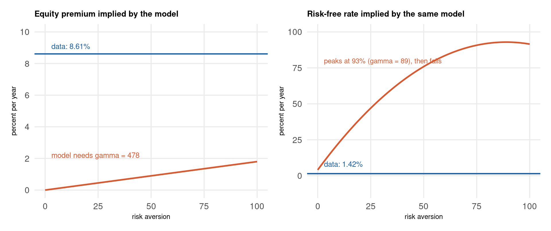
The model premium is 0.036% a year against 8.61% in the data — smaller by a factor of 239, more than two orders of magnitude. And it produces that failure while simultaneously setting a risk-free rate almost six times too high.
This is not a calibration accident. Every parameter on the previous slide was chosen to flatter the model, including a consumption-return correlation of 0.20 when the data say 0.061.
Look at the two panels together — that is the whole argument.
The premium is linear in risk aversion with a tiny slope, because it is \(\gamma\rho\sigma_c\sigma_d\) and the last three terms multiply to almost nothing. To reach the data’s 8.61% you need \(\gamma = 478\).
The risk-free rate is quadratic in risk aversion, and rises far faster. At \(\gamma = 478\) the same model implies a risk-free rate of \(-1613\%\) per year. Long before that it has passed through absurdity: at \(\gamma = 50\) the premium is still only 0.9% while the risk-free rate is already 76%.
There is no value of \(\gamma\) that fixes both. The failure is structural, not numerical: one parameter is being asked to set the price of risk and the level of rates, and those two jobs pull in opposite directions.
The rest of Part 3 is a catalogue of ways out. Epstein–Zin unties the two jobs by giving the model a second preference parameter. Long-run risk and habit make consumption riskier than it looks. Disasters argue the sample never showed us the risk that was actually being priced.
The previous slide ended on a structural complaint: one parameter is doing two jobs. Under CRRA, \(\gamma\) measures both how much you dislike risk across states and how much you dislike variation across time. They are forced to be reciprocals:
\[\psi = \frac{1}{\gamma}\]
There is no reason for that. A consumer might hate gambles yet be happy to substitute consumption between this year and next. Epstein and Zin (1989) build a recursive utility that separates the two, and it costs exactly one extra parameter.
The price of that parameter is structural, not just numerical: utility becomes recursive, so the continuation value enters the pricing kernel. That is the whole novelty — and it is the door long-run risk walks through two slides from now.
It also introduces something CRRA does not have: a preference over when uncertainty is resolved. That turns out to matter enormously — but, as the tabs opposite show, only once consumption growth is predictable.
The one line of algebra that explains the result
Write
\[\theta = \frac{1-\gamma}{1-1/\psi}\]
so that \(\psi = 1/\gamma\) gives \(\theta = 1\) and collapses everything back to CRRA. In the i.i.d. Lucas world the wealth-consumption ratio is a constant, and the log kernel reduces to
\[m_{t+1} = A - \gamma \, \Delta c_{t+1}\]
The slope on consumption growth is still \(-\gamma\), so the premium cannot move. Only the intercept \(A\) — and hence the risk-free rate — responds to \(\psi\).
Everything is closed form here, so both code tabs print the same numbers to every digit. The two rows to compare are the CRRA benchmark\(\psi = 1/\gamma\) and anything else.
Recursive utility has no Stata implementation — nothing built in, nothing on SSC — so Stata rejoins the deck at the long-run risk slides, where the object being solved is a finite Markov chain it handles natively.
Read down the premium column: it does not move. At \(\gamma = 10\) the premium is 0.1800% whether \(\psi\) is 0.1 or 2.0, while the risk-free rate falls from 22.90% to 4.86%. Epstein–Zin solves the risk-free rate puzzle outright and contributes nothing whatsoever to the equity premium puzzle.
That is not a disappointment — it is a signpost. The kernel’s slope on consumption growth is still \(-\gamma\) because, with i.i.d. growth, next period’s continuation value carries no information. Give consumption growth a persistent component and that stops being true.
Bansal and Yaron (2004) take the signpost from the last slide seriously. Suppose consumption growth contains a small, highly persistent, barely visible component:
\(x_t\) explains almost none of the one-period variance of consumption growth — it is nearly undetectable in a century of data. But with \(\rho = 0.979\) monthly, a shock to \(x\) moves expected consumption for decades.
An Epstein–Zin consumer with \(\psi > 1\) cares about that, because bad news about the distant future lowers her continuation value today. Assets that fall when \(x\) falls are therefore genuinely risky, and command a premium — even though their correlation with current consumption growth is negligible, exactly as measured in Part 1.
The full system, monthly, with a levered dividend claim:
with \(\eta, e, u\) independent. Instead of log-linearising, we discretise \(x\) with Rouwenhorst — the method Part 2 showed is exact at this persistence — and solve two fixed points on the resulting 9-state chain.
The kernel then takes the convenient form \(M_{t+1} = \beta \, G^{-\gamma} \, v_j^{1/\psi-\gamma} X_i^{\gamma-1/\psi}\), where \(G\) is consumption growth and \(X_i\) the certainty equivalent. The price-dividend ratio is linear in itself:
The \(v\) fixed point is iterated a fixed 2000 times in all three languages rather than to a tolerance, so the algorithm is deterministic and every tab prints the same digits. The price-dividend ratio is then solved exactly as a linear system.
Code
gamma <-10; psi <-1.5; beta <-0.998mu <-0.0015; sig <-0.0078; rho <-0.979; phie <-0.044mud <-0.0015; phi <-3.0; phid <-4.5g <-rouwenhorst(9, rho, phie * sig) # from Part 2 -- exact at this rhox <- g$z; P <- g$P# 1. utility-consumption ratio, by fixed pointv <-rep(1, 9)sup <-numeric(2000) # sup-norm of each update -- the convergence profilefor (it in1:2000) { inner <-exp((1- gamma) * (mu + x) +0.5* (1- gamma)^2* sig^2) *as.vector(P %*% (v^(1- gamma))) vnew <- ((1- beta) + beta * inner^((1-1/psi) / (1- gamma)))^(1/ (1-1/psi)) sup[it] <-max(abs(vnew - v)) v <- vnew}X <- (exp((1- gamma) * (mu + x) +0.5* (1- gamma)^2* sig^2) *as.vector(P %*% (v^(1- gamma))))^(1/ (1- gamma))EG <-exp(-gamma * (mu + x) +0.5* gamma^2* sig^2)EDg <-exp(mud + phi * x +0.5* phid^2* sig^2)w <- v^(1/psi - gamma)# 2. price-dividend ratio, solved exactly as a linear systemcc <- beta * X^(gamma -1/psi) * EG * EDgA <-outer(cc, rep(1, 9)) * P *outer(rep(1, 9), w)p <-solve(diag(9) - A, A %*%rep(1, 9))Rf <-1/ (beta * X^(gamma -1/psi) * EG *as.vector(P %*% w))ER <-as.vector(P %*% (1+ p)) /as.vector(p) * EDg
Long-run risk, 9-state Rouwenhorst chain, 2000 iterations

  equity premium          5.0397 % per year
  risk-free rate          2.6052 % per year
  price-dividend          269.73

  P/D across states   176.5 (worst x) to 408.0 (best x)

  convergence profile, sup-norm |v(k+1) - v(k)|
    k =   100    9.348e-04
    k =   500    7.014e-05
    k =  1000    2.648e-05
    k =  2000    3.717e-06
Code
import numpy as npgamma, psi, beta =10.0, 1.5, 0.998mu, sig, rho, phie =0.0015, 0.0078, 0.979, 0.044mud, phi, phid =0.0015, 3.0, 4.5x, P = rouwenhorst(9, rho, phie * sig) # from Part 2 -- exact at this rho# 1. utility-consumption ratio, by fixed pointv = np.ones(9)sup = np.zeros(2000) # sup-norm of each update -- the convergence profilefor it inrange(2000): inner = (np.exp((1-gamma)*(mu + x) +0.5*(1-gamma)**2*sig**2)* (P @ v**(1-gamma))) vnew = ((1-beta) + beta*inner**((1-1/psi)/(1-gamma)))**(1/(1-1/psi)) sup[it] = np.abs(vnew - v).max() v = vnewX = (np.exp((1-gamma)*(mu + x) +0.5*(1-gamma)**2*sig**2)* (P @ v**(1-gamma)))**(1/(1-gamma))EG = np.exp(-gamma*(mu + x) +0.5*gamma**2*sig**2)EDg = np.exp(mud + phi*x +0.5*phid**2*sig**2)w = v**(1/psi - gamma)# 2. price-dividend ratio, solved exactly as a linear systemcc = beta * X**(gamma -1/psi) * EG * EDgA = cc[:, None] * P * w[None, :]p = np.linalg.solve(np.eye(9) - A, A @ np.ones(9))Rf =1/ (beta * X**(gamma -1/psi) * EG * (P @ w))ER = (P @ (1+ p)) / p * EDgev, evec = np.linalg.eig(P.T)pr = np.real(evec[:, np.argmax(np.real(ev))]); pr = pr / pr.sum()out = ("Long-run risk, 9-state Rouwenhorst chain, 2000 iterations\n\n"f" equity premium {1200*(pr*(ER-Rf)).sum():10.4f} % per year\n"f" risk-free rate {1200*(pr*np.log(Rf)).sum():10.4f} % per year\n"f" price-dividend {(pr*p).sum():10.2f}\n"f"\n P/D across states {p.min():.1f} (worst x) to {p.max():.1f} (best x)\n""\n convergence profile, sup-norm |v(k+1) - v(k)|\n")for k in (100, 500, 1000, 2000): out +=f" k = {k:5d}{sup[k-1]:10.3e}\n"import sys; nchars = sys.stdout.write(out); sys.stdout.flush()
Long-run risk, 9-state Rouwenhorst chain, 2000 iterations

  equity premium          5.0397 % per year
  risk-free rate          2.6052 % per year
  price-dividend          269.73

  P/D across states   176.5 (worst x) to 408.0 (best x)

  convergence profile, sup-norm |v(k+1) - v(k)|
    k =   100    9.348e-04
    k =   500    7.014e-05
    k =  1000    2.648e-05
    k =  2000    3.717e-06
Long-run risk, 9-state Rouwenhorst chain, 2000 iterations

  equity premium          5.0397 % per year
  risk-free rate          2.6052 % per year
  price-dividend          269.73

  P/D across states   176.5 (worst x) to 408.0 (best x)

  convergence profile, sup-norm |v(k+1) - v(k)|
    k =   100    9.348e-04
    k =   500    7.014e-05
    k =  1000    2.648e-05
    k =  2000    3.717e-06
A fixed iteration count is a parity choice, not a convergence criterion — and this one has not converged. In real work you stop on a tolerance: iterate until \(\lVert v^{(k+1)} - v^{(k)} \rVert_\infty\) falls below something you chose, and report the \(k\) it took. The profile printed above is what that rule would have seen, and it is sobering: the update is still moving by \(3.7 \times 10^{-6}\) at \(k = 2000\), and the sup-norm does not fall below \(10^{-12}\) until \(k = 9684\) — nearly five times the iteration count this slide uses.
It costs almost nothing here. Running to \(10^{-12}\) moves the equity premium from \(5.0397\) to \(5.0399\) and the price-dividend ratio from \(269.73\) to \(269.72\) — the fourth significant digit, invisible at the precision the results slide quotes. But that is a fact discovered by measuring, not a fact anyone should assume.
Fixed iteration counts buy cross-language determinism; tolerances buy a correctness guarantee. Know which one you are using, and never let a fixed count stand in for a convergence check you did not run.
From a factor of 239 away to a factor of 1.7. The same model simultaneously brings the risk-free rate down from 7.98% to 2.61%, against 1.42% in the data. Both puzzles move in the right direction at once — which is exactly what no amount of raising \(\gamma\) in the Lucas tree could achieve.
And it does so with a persistent component that is nearly invisible: \(x_t\) accounts for well under 1% of the one-month variance of consumption growth.
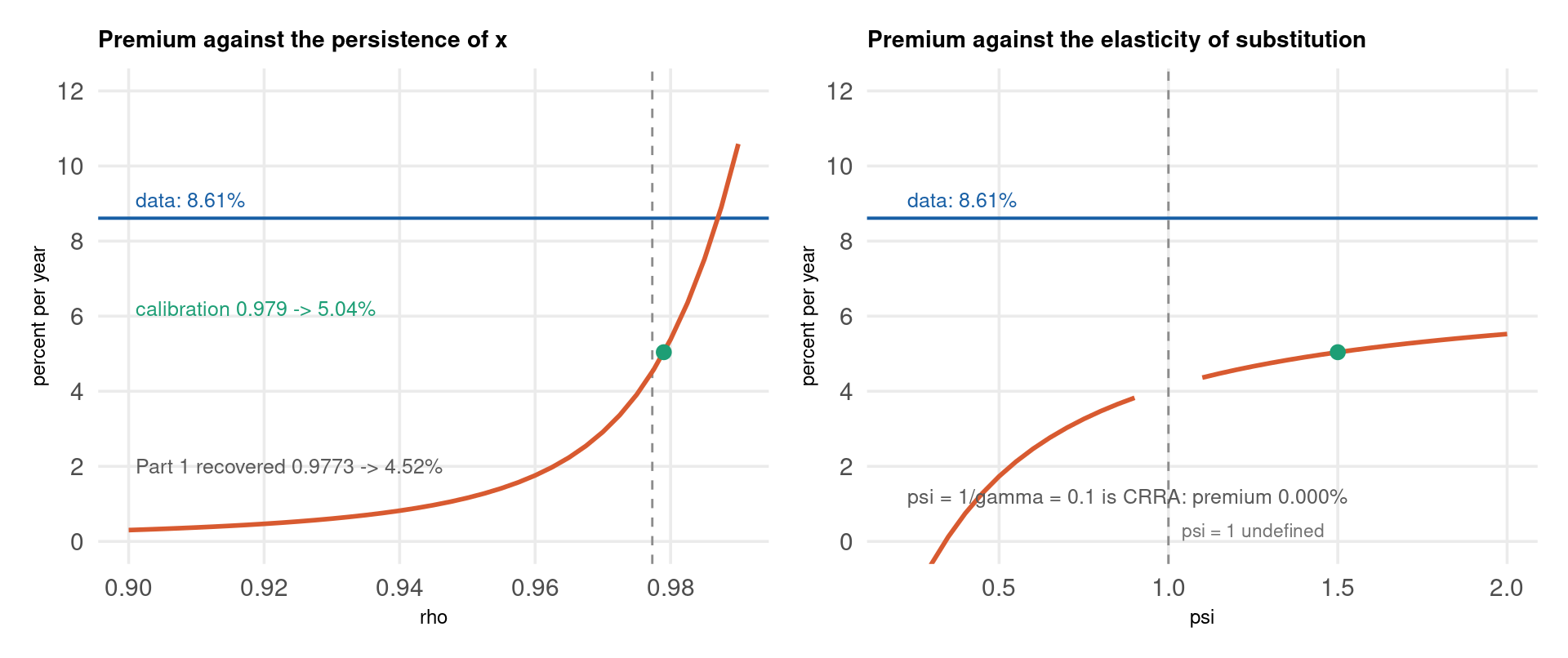
change
premium
what it means
\(\rho = 0.979\) (calibration)
5.04%
the headline result
\(\rho = 0.9773\)
4.52%
the value Part 1’s own diagnostics recovered from 3000 simulated months
\(\rho = 0.95\)
1.16%
still “highly persistent” by any normal standard
\(\rho = 0.90\)
0.30%
back to the Lucas tree
\(\psi = 1/\gamma = 0.1\) (CRRA)
0.000%
long-run risk prices nothing at all under expected utility
\(\psi = 0.5\)
1.73%
\(\psi < 1\) guts the mechanism
\(\gamma = 5\)
2.69%
still needs high risk aversion
Two things here deserve to be said plainly.
(\(\psi = 1\) itself is left out of the figure: \(\theta = (1-\gamma)/(1-1/\psi)\) is undefined there, and the log-utility case has to be taken as a limit.)
First, \(\psi\) must exceed 1. At \(\psi = 1/\gamma\) the model is CRRA, and the premium is exactly zero — long-run risk contributes nothing without a preference for early resolution of uncertainty. The mechanism is Epstein–Zin’s, not the persistence’s; persistence only gives it something to bite on.
Second, and more uncomfortable: the answer hinges on a parameter nobody can measure. Moving \(\rho\) from 0.979 to 0.95 cuts the premium by a factor of four. And Part 1’s diagnostics, run on 3000 months simulated from a process with \(\rho = 0.979\), recovered 0.9773 — because the AR(1) coefficient is biased downward near a unit root. That estimate alone costs half a percentage point of premium.
This is the Beeler–Campbell (2012) critique in one figure: the model works, but the parameter it works through is estimated with an uncertainty far wider than the range over which the answer changes completely. Part 7 returns to this as a weak identification problem rather than a calibration quibble.
Long-run risk made consumption riskier than it looks. Campbell and Cochrane (1999) take the other route: leave consumption alone and make the consumer’s attitude to risk move with the cycle.
The consumer cares about consumption relative to a slow-moving habit \(X_t\). What matters is the surplus
\[S_t = \frac{C_t - X_t}{C_t}\]
In good times \(C\) is far above habit, \(S\) is large, and a given consumption shock barely matters. In bad times \(C\) is close to habit, \(S\) is small, and the same shock is nearly catastrophic. Effective risk aversion is \(\gamma / S_t\) — it rises exactly when the economy is weak.
This delivers something neither previous model does: a time-varying price of risk. Part 1’s stylised fact 3 said risk is not constant. Habit is the first model in this deck that agrees.
The surplus is the fraction of consumption that sits above habit,
\[S_t = \frac{C_t - X_t}{C_t}\]
and effective risk aversion is \(\gamma / S_t\), so it rises exactly when the economy is weak. Log surplus follows a heteroskedastic AR(1) — the whole model, computationally:
The sensitivity function \(\lambda(s_t)\) is not a free choice. Campbell and Cochrane (1999) pick the one shape that holds the risk-free rate constant, so that every bit of the model’s action sits in the price of risk rather than in the interest rate; the code tab carries the resulting formula.
The discount factor is CRRA in the surplus-scaled growth rate,
Annual calibration: \(g = 0.0189\), \(\sigma = 0.0150\), \(\varphi = 0.87\), \(\gamma = 2\). So the thing to compute is a state-dependent heteroskedastic AR(1), simulated for 100 000 periods, and the number to score is \(\sqrt{2 \times 0.13}\) against the annual Sharpe ratio of \(0.525\) measured in Part 1.
Campbell-Cochrane habit, annual calibration

  steady-state surplus S-bar          0.0588
  max Sharpe at steady state          0.5099   = sqrt(gamma(1-phi))
  US data, annual Sharpe (Part 1)     0.5250

  simulated Sharpe: mean 0.455   10th pct 0.170   90th pct 0.774
  surplus S_t:      mean 0.0644  10th pct 0.0306  90th pct 0.0918
Code
import numpy as npg, sg, phi_h, gam =0.0189, 0.0150, 0.87, 2.00Sbar = sg * np.sqrt(gam / (1- phi_h))sbar = np.log(Sbar)smax = sbar + (1- Sbar**2) /2def lam(s): inside =max(1-2* (s - sbar), 0.0)return (1/ Sbar) * np.sqrt(inside) -1if s <= smax else0.0rng = np.random.default_rng(14159)n =100000s = np.empty(n); s[0] = sbarfor i inrange(1, n): e = rng.normal(0, sg) s[i] = (1- phi_h) * sbar + phi_h * s[i-1] + lam(s[i-1]) * esharpe = gam * sg * (1+ np.array([lam(si) for si in s]))out = ("Campbell-Cochrane habit, annual calibration\n\n"f" steady-state surplus S-bar {Sbar:8.4f}\n"f" max Sharpe at steady state {np.sqrt(gam*(1-phi_h)):8.4f}"" = sqrt(gamma(1-phi))\n"f" US data, annual Sharpe (Part 1) {0.525:8.4f}\n\n"f" simulated Sharpe: mean {sharpe.mean():.3f} "f"10th pct {np.quantile(sharpe,0.10):.3f} "f"90th pct {np.quantile(sharpe,0.90):.3f}\n"f" surplus S_t: mean {np.exp(s).mean():.4f} "f"10th pct {np.quantile(np.exp(s),0.10):.4f} "f"90th pct {np.quantile(np.exp(s),0.90):.4f}\n")import sys; nchars = sys.stdout.write(out); sys.stdout.flush()
Campbell-Cochrane habit, annual calibration

  steady-state surplus S-bar          0.0588
  max Sharpe at steady state          0.5099   = sqrt(gamma(1-phi))
  US data, annual Sharpe (Part 1)     0.5250

  simulated Sharpe: mean 0.452   10th pct 0.169   90th pct 0.766
  surplus S_t:      mean 0.0647  10th pct 0.0314  90th pct 0.0918
\(\sqrt{\gamma(1-\varphi)} = \sqrt{2 \times 0.13} = 0.510\), against a measured annual Sharpe ratio of 0.525. Habit clears the Hansen–Jagannathan bound of Part 1 at \(\gamma = 2\) — the value the Lucas tree needed 478 of. And it does so with a price of risk that ranges from 0.17 in good times to 0.77 in bad, which is the countercyclical variation Part 1’s third stylised fact demanded.
Rietz (1988) and Barro (2006) make a different objection: the sample is the problem, not the model. Suppose consumption is normally smooth but occasionally collapses — war, depression, financial ruin — by 10 to 70%, with probability about 1.7% a year. Investors price that risk continuously. A researcher looking at 79 years of US data mostly does not see it.
A disaster raises \(M\) enormously — \((1-b)^{-\gamma}\) with \(b = 0.3\) and \(\gamma = 4\) is a factor of 4 — precisely when the levered claim collapses. That covariance is the premium, and it needs no implausible risk aversion at all.
Rare disasters, gamma = 4, p = 0.017

  population premium                  4.303 % per year
  risk-free rate                      4.992 % per year

  79-year samples with NO disaster     26.6 %
  measured premium, all samples       4.301 %
  measured premium, disaster-free     5.410 %
  measured premium, with disaster     3.899 %
  sd of the measured premium          1.236 %
Code
import numpy as nprng = np.random.default_rng(14159)p_d, gam_d, beta_d, mu_d, sc_d =0.017, 4, 0.99, 0.025, 0.02NB =2000000J = rng.binomial(1, p_d, NB)b = np.zeros(NB)b[J ==1] = rng.beta(2, 5, J.sum()) *0.6+0.10dc = mu_d + sc_d * rng.normal(size=NB) + np.log(1- b)sdf = beta_d * np.exp(-gam_d * dc)Rf =1/ sdf.mean()dd = mu_d +3* sc_d * rng.normal(size=NB) +3* np.log(1- b)Rm = np.exp(dd) / (sdf * np.exp(dd)).mean()# The peso problem: what does a 79-year sample actually measure?Ns, R =79, 20000idx = rng.integers(0, NB, size=(R, Ns))est = Rm[idx].mean(axis=1) - Rfnodis = (J[idx] ==0).all(axis=1)out = (f"Rare disasters, gamma = {gam_d}, p = {p_d:.3f}\n\n"f" population premium {100*(Rm.mean()-Rf):8.3f} % per year\n"f" risk-free rate {100*np.log(Rf):8.3f} % per year\n"f"\n 79-year samples with NO disaster {100*nodis.mean():8.1f} %\n"f" measured premium, all samples {100*est.mean():8.3f} %\n"f" measured premium, disaster-free {100*est[nodis].mean():8.3f} %\n"f" measured premium, with disaster {100*est[~nodis].mean():8.3f} %\n"f" sd of the measured premium {100*est.std(ddof=1):8.3f} %\n")import sys; nchars = sys.stdout.write(out); sys.stdout.flush()
Rare disasters, gamma = 4, p = 0.017

  population premium                  4.284 % per year
  risk-free rate                      5.015 % per year

  79-year samples with NO disaster     26.1 %
  measured premium, all samples       4.290 %
  measured premium, disaster-free     5.397 %
  measured premium, with disaster     3.899 %
  sd of the measured premium          1.233 %
A premium of 4.3% at \(\gamma = 4\) — from a model in which nothing about preferences is strange. But look at the last three lines: 27% of 79-year samples contain no disaster at all, and in those the measured premium is 5.4% against a population value of 4.3%. The sample overstates by a quarter, purely because the risk being priced never showed up.
That is the peso problem, and it cuts both ways. The disaster story explains the premium and explains why the premium looks even larger than it is — but it does so with a parameter, \(p\), that the data by construction can barely identify. Part 7 asks what that does to estimation.
Model Horse Race
Every number below was computed on a slide in this part. None is quoted from a paper.
Habit is scored on the maximum Sharpe ratio rather than a premium: the model delivers the price of risk analytically, and pinning down a premium would require solving the price-dividend ratio over the surplus state.
No model wins outright, and the two that come closest do so for opposite reasons. Long-run risk and disasters both say the data understate the risk — one because it is too persistent to see in a short sample, the other because it is too rare. Habit says the risk is visible enough; it is the price that moves. All three are consistent with Part 1’s measurements. That is precisely why distinguishing them is a Part 7 problem, not a Part 3 one.
          model gamma premium   rf sharpe   gap
        US data    NA    8.61 1.42  0.525  0.00
     Lucas tree     2    0.04 7.98  0.020 -8.57
    Epstein-Zin    10    0.18 5.17  0.080 -8.43
  Long-run risk    10    5.04 2.61     NA -3.57
          Habit     2      NA   NA  0.510    NA
 Rare disasters     4    4.30 4.99     NA -4.31
         model  gamma  premium   rf  sharpe   gap
       US data    NaN     8.61 1.42   0.525  0.00
    Lucas tree    2.0     0.04 7.98   0.020 -8.57
   Epstein-Zin   10.0     0.18 5.17   0.080 -8.43
 Long-run risk   10.0     5.04 2.61     NaN -3.57
         Habit    2.0      NaN  NaN   0.510   NaN
Rare disasters    4.0     4.30 4.99     NaN -4.31
Parts 1 to 3 priced assets in an endowment economy: consumption fell from the sky and the only question was what it was worth. That is the right laboratory for the equity premium, and the wrong one for almost everything a central bank cares about.
Now production returns. Output is made with capital, capital is accumulated by forgoing consumption, and a technology shock propagates through the whole system because today’s saving is tomorrow’s capital. The model becomes dynamic in a second sense: not just expectations of the future, but a physical state that carries the past forward.
This is the model that generated mfsim-dsge.csv in Part 1. Its policy coefficients were published there — \(g_k = 0.618247\), \(g_a = 0.305243\), \(A_k = 0.965276\). This part has to rediscover them from scratch, by a completely different route, in three languages. If the numbers come back, both the data script and the solver are right.
A real business cycle model with fixed labour and log utility. In log deviations from steady state, with \(k\) capital, \(a\) technology and \(c\) consumption:
The three equations above are not a recursion you can simulate. Two of them involve \(\mathbb{E}_t[\,\cdot_{t+1}]\), and there are infinitely many paths satisfying them — most of which explode. Choosing among them is the entire content of “solving” a rational expectations model.
The rule that picks the right one is due to Blanchard and Kahn: a unique non-explosive solution exists iff the number of unstable roots equals the number of forward-looking variables. Here there are two predetermined variables (\(k\), \(a\)) and one jump variable (\(c\)), so we need exactly one root outside the unit circle.
What happens when the count is wrong
Too few unstable roots and the model has many solutions — indeterminacy, with sunspots. Too many and it has none.
The count is not a technicality to be assumed; it is a property of the calibration, and the code on the next slide reports it rather than trusting it.
Stack \(x_t = (k_t, a_t, c_t)'\) and write the system as a linear pencil:
\(\mathbf{A}\) is singular in general, so ordinary eigenvalues will not do. The generalized Schur (QZ) decomposition finds unitary \(Q, Z\) with
\[Q \mathbf{B} Z = S, \qquad Q \mathbf{A} Z = T\]
both upper triangular, and the generalized eigenvalues are \(\lambda_i = S_{ii}/T_{ii}\), reordered so the stable ones come first. Partitioning \(Z\) conformably with the \(n_k = 2\) states, Klein’s (2000) solution is
Three genuinely different routes to the same object: R and Python build the pencil and call a generalized Schur routine directly; Stata states the model in dsge syntax and reads the answer off estat policy.
Generalized eigenvalues (stable first): 0.965276  0.950000  1.046437
Blanchard-Kahn: 1 unstable root(s), 1 jump variable(s)  -> unique stable solution

  policy    g_k = 0.618247    truth 0.618247
            g_a = 0.305243    truth 0.305243
  transition A_k = 0.965276    truth 0.965276
            B_a = 0.075372    truth 0.075372
          rho_a = 0.950000    truth 0.950000
Code
import numpy as npimport pandas as pdfrom scipy.linalg import ordqzalpha, bta, delta, rho_a =0.36, 0.99, 0.025, 0.95ky = alpha / (1/bta -1+ delta)phi =1/ky; s_i = delta*ky; s_c =1- s_ichi = bta*alpha*phia0 = (1- delta) + phi*alphaA = np.array([[1.0, 0, 0], [0, 1.0, 0], [-chi*(alpha-1), 0, 1.0]])B = np.array([[a0, phi, -phi*s_c], [0, rho_a, 0], [0, chi*rho_a, 1.0]])# sort='iuc' puts the roots INSIDE the unit circle firstS, T, al, be, Q, Z = ordqz(B, A, sort="iuc", output="real")lam = np.real(al / be)nk =2# k and a are predeterminedZ11 = Z[:nk, :nk]; Z21 = Z[nk:, :nk]S11 = S[:nk, :nk]; T11 = T[:nk, :nk]F = Z21 @ np.linalg.inv(Z11) # c_t = F (k_t, a_t)'P = Z11 @ np.linalg.solve(T11, S11) @ np.linalg.inv(Z11) # state transitiontruth = pd.read_csv("../data/mfsim-dsge.csv")nun =int((np.abs(lam) >=1).sum())out = ("Generalized eigenvalues (stable first): "+" ".join(f"{v:.6f}"for v in lam) +"\n"f"Blanchard-Kahn: {nun} unstable root(s), 1 jump variable(s) -> "+ ("unique stable solution"if nun ==1else"FAILS") +"\n\n"f" policy g_k = {F[0,0]:.6f} truth {truth['gk_true'][0]:.6f}\n"f" g_a = {F[0,1]:.6f} truth {truth['ga_true'][0]:.6f}\n"f" transition A_k = {P[0,0]:.6f} truth {truth['Ak_true'][0]:.6f}\n"f" B_a = {P[0,1]:.6f} truth {0.075372:.6f}\n"f" rho_a = {P[1,1]:.6f} truth {truth['rhoa_true'][0]:.6f}\n")import sys; nchars = sys.stdout.write(out); sys.stdout.flush()
Generalized eigenvalues (stable first): 0.965276  0.950000  1.046437
Blanchard-Kahn: 1 unstable root(s), 1 jump variable(s)  -> unique stable solution

  policy    g_k = 0.618247    truth 0.618247
            g_a = 0.305243    truth 0.305243
  transition A_k = 0.965276    truth 0.965276
            B_a = 0.075372    truth 0.075372
          rho_a = 0.950000    truth 0.950000
Code
quietly { import delimited "../data/mfsim-dsge.csv", cleartsset t * every structural parameter is known, so rho is pinned by a constraint * and dsge solves rather than estimatesconstraint 1 _b[/structural:rho] = 0.95 dsge (c = E(F.c) - .0347500000*F.a + .0222400000*F.k) /// (F.k = 1.0101010101*k + .0975028058*a - .0725028058*c, /// state noshock) /// (F.a = {rho=.95}*a, state), constraints(1)}estat policyestat transition
Policy matrix

------------------------------------------------------------------------------
             |            Delta-method
             | Coefficient  std. err.      z    P>|z|     [95% conf. interval]
-------------+----------------------------------------------------------------
c            |
           k |   .6182466          .        .       .            .           .
           a |    .305243          .        .       .            .           .
------------------------------------------------------------------------------
Note: Standard errors reported as missing for constrained policy matrix values.


Transition matrix of state variables

------------------------------------------------------------------------------
             |            Delta-method
             | Coefficient  std. err.      z    P>|z|     [95% conf. interval]
-------------+----------------------------------------------------------------
F.k          |
           k |   .9652764          .        .       .            .           .
           a |   .0753718          .        .       .            .           .
-------------+----------------------------------------------------------------
F.a          |
           k |          0  (omitted)
           a |        .95          .        .       .            .           .
------------------------------------------------------------------------------
Note: Standard errors reported as missing for constrained transition matrix values.
Stata reaches the same solution from the other end: dsge takes the model in its structural form, forms the pencil internally, checks the Blanchard–Kahn count and reports the policy matrix (\(c\) on the states) and the transition matrix (states on states) directly.
Three routes, one answer, and it is the right one. The generalized eigenvalues are \(0.965276\), \(0.950000\) and \(1.046437\) — exactly one outside the unit circle for exactly one jump variable, so Blanchard–Kahn holds and the solution is unique. The recovered policy \(g_k = 0.6182\), \(g_a = 0.3052\) and transition \(A_k = 0.9653\), \(B_a = 0.0754\) match the values mfsim-data.R published in Part 1 to five decimal places — and note that the data script got there by solving a quadratic by hand, not by QZ at all. Two independent methods, same numbers.
quietly { import delimited "../data/mfsim-dsge.csv", cleartsset tconstraint 1 _b[/structural:rho] = 0.95 dsge (c = E(F.c) - .0347500000*F.a + .0222400000*F.k) /// (F.k = 1.0101010101*k + .0975028058*a - .0725028058*c, /// state noshock) /// (F.a = {rho=.95}*a, state), constraints(1) * pull the solved matrices straight out of the estat resultsestat policymatrix POL = r(b)estat transitionmatrix TRN = r(b)scalar gk = POL[1,1]scalar ga = POL[1,2]scalar Ak = TRN[1,1]scalar Ba = TRN[1,2]scalar ra = TRN[1,4]scalaralpha = 0.36scalar s_c = 0.7435971223scalar s_i = 0.2564028777clearsetobs 40generateh = _n - 1generatedouble kk = 0generatedouble aa = 0replace aa = 1 in 1forvalues j = 2/40 {replace kk = Ak*kk[`j'-1] + Ba*aa[`j'-1] in`j'replace aa = ra*aa[`j'-1] in`j' }generatedoublecc = gk*kk + ga*aageneratedouble yy = aa + alpha*kkgeneratedouble ii = (yy - s_c*cc)/s_i}twoway (line ii h, lcolor("216 90 48") lwidth(medium)) /// (line yy h, lcolor("24 95 165") lwidth(medium)) /// (line kk h, lcolor("29 158 117") lwidth(medium)) /// (linecch, lcolor("186 117 23") lwidth(medium)), ///yline(0, lcolor(gs11) lwidth(vthin)) ///xscale(range(0 39)) yscale(range(-0.2 3.2)) ///xlabel(0(10)40) ylabel(0(1)3) ///xtitle("quarters") ytitle("percent deviation") ///title("Response to a 1% technology shock", size(medsmall)) ///text(2.85 6 "investment", color("216 90 48") size(vsmall) /// placement(e) justification(left)) ///text(0.92 12 "output", color("24 95 165") size(vsmall) /// placement(e) justification(left)) ///text(0.70 20 "capital", color("29 158 117") size(vsmall) /// placement(e) justification(left)) ///text(0.30 20 "consumption", color("186 117 23") size(vsmall) /// placement(e) justification(left)) ///legend(off) graphregion(color(white))graphexport"../plots/mfsim-irf-stata.png", replacewidth(1600)
Reading the impulse responses
Investment peaks at 3.0% on impact, three times the size of the shock; consumption rises only 0.53% and then keeps rising as capital accumulates. That split — volatile investment, smooth consumption, both hump-shaped through capital — is the RBC mechanism in one picture. The Stata tab reaches the same figure by pulling \(F\) and \(P\) out of estat policy and estat transition rather than re-deriving them.
Stochastic Simulation & Model Moments
Rather than simulating live — which would give three different answers — every tab reads the 1000 quarters already in mfsim-dsge.csv, produced by this model at these parameters, and compares them with mfsim-macro.csv. Both are quarterly log growth rates, so the comparison is like for like.
Code
md <-read.csv("../data/mfsim-dsge.csv")us <-read.csv("../data/mfsim-macro.csv")# model series are in percent deviations; differencing gives growth ratesdy <-diff(md$y) /100; dc <-diff(md$c) /100; di <-diff(md$i) /100ey <- us$dgdp /400; ec <- us$dcons /400# dcons is 400 x log-diffmoments <-function(gy, gc, gi =NULL) { n <-length(gy)c(sd_y =100*sd(gy),rel_c =sd(gc) /sd(gy),rel_i =if (is.null(gi)) NAelsesd(gi) /sd(gy),cor_cy =cor(gc, gy),ac1_y =cor(gy[-1], gy[-n]))}mm <-moments(dy, dc, di)uu <-moments(ey, ec)
                moment model  data
 sd(dy), % per quarter 0.723 1.105
         sd(dc)/sd(dy) 0.315 0.966
         sd(di)/sd(dy) 3.043    NA
          corr(dc, dy) 0.953 0.735
               ac1(dy) 0.001 0.134
Code
import numpy as npimport pandas as pdmd = pd.read_csv("../data/mfsim-dsge.csv")us = pd.read_csv("../data/mfsim-macro.csv")# model series are in percent deviations; differencing gives growth ratesdy = np.diff(md["y"]) /100; dc = np.diff(md["c"]) /100; di = np.diff(md["i"]) /100ey = us["dgdp"].to_numpy() /400; ec = us["dcons"].to_numpy() /400def moments(gy, gc, gi=None):return [100* gy.std(ddof=1), gc.std(ddof=1) / gy.std(ddof=1), np.nan if gi isNoneelse gi.std(ddof=1) / gy.std(ddof=1), np.corrcoef(gc, gy)[0, 1], np.corrcoef(gy[1:], gy[:-1])[0, 1]]mm = moments(dy, dc, di)uu = moments(ey, ec)tab = pd.DataFrame({"moment": ["sd(dy), % per quarter", "sd(dc)/sd(dy)", "sd(di)/sd(dy)","corr(dc, dy)", "ac1(dy)"],"model": np.round(mm, 3),"data": np.round(uu, 3)})import sys; nchars = sys.stdout.write(tab.to_string(index=False) +"\n")
               moment  model  data
sd(dy), % per quarter  0.723 1.105
        sd(dc)/sd(dy)  0.315 0.966
        sd(di)/sd(dy)  3.043   NaN
         corr(dc, dy)  0.953 0.735
              ac1(dy)  0.001 0.134
               moment      model       data
sd(dy), % per quarter      0.723      1.105
        sd(dc)/sd(dy)      0.315      0.966
        sd(di)/sd(dy)      3.043         NA
         corr(dc, dy)      0.953      0.735
              ac1(dy)      0.001      0.134
Where the RBC model wins and where it does not. It gets the shape right — investment three times as volatile as output, consumption smoother, both strongly procyclical. But consumption is far too smooth: the model says \(\sigma(\Delta c)/\sigma(\Delta y) = 0.32\) where the data say 0.97. Real households smooth almost nothing at quarterly frequency, and a frictionless permanent-income consumer smooths almost everything. The model also generates no growth persistence (ac1 of 0.00 against 0.13) because all the propagation runs through capital, which moves too slowly to show up in one quarter.
Part 3 spent eleven slides on the price of risk. This model has capital, a consumption Euler equation and a stochastic shock — everything needed to price risk. Yet its equity premium is exactly zero, and not because the calibration is unlucky.
A first-order perturbation is a Taylor expansion of the policy function around the deterministic steady state, taken to first order in the states and in the shock scale \(\sigma\):
It is a theorem that \(g_\sigma = 0\): to first order the agent behaves exactly as she would if the future were certain. This is certainty equivalence, and it has a sharp, testable implication —
the first-order solution matrices \(F\) and \(P\)do not contain \(\sigma_a\) at all. Multiply the volatility of the economy by ten and the decision rules do not move by one bit.
In consequence the model’s own risk-free rate and expected return on capital coincide. From the Euler equation, the riskless rate is \(r^f_t = \mathbb{E}_t[c_{t+1}] - c_t\), while the return on capital satisfies \(c_t = \mathbb{E}_t[c_{t+1}] - \mathbb{E}_t[r_{t+1}]\), so
identically, period by period, at every state. Risk premia are second-order objects: they are \(O(\sigma^2)\), and a first-order solution has thrown that term away before the question is asked.
Code
# 1. Certainty equivalence: solve the model at two very different volatilitiessolve_rbc <-function(sig_a) {# sig_a never enters A or B -- that is the whole point ... # identical to the Part 4 solverlist(F = Fm, P = Pm)}m_low <-solve_rbc(0.007)m_high <-solve_rbc(0.070) # ten times as volatile# 2. The model's own risk premium, state by stateErk <- chi * (rho_a * s[, 2] + (alpha -1) * knext) # E_t[return on capital]rf <- Ec1 - c_sim # E_t[c_{t+1}] - c_tprem <- Erk - rf
1. Certainty equivalence -- solve at sigma_a = 0.007 and 0.070
     max |F(low) - F(high)|   0.000e+00
     max |P(low) - P(high)|   0.000e+00

2. The model's own risk premium over 1000 simulated quarters
     mean premium             -3.488e-18
     max |premium|            3.009e-17
     machine epsilon          2.220e-16
Code
import numpy as npfrom scipy.linalg import ordqzdef solve_rbc(sig_a): al, bt, dl, ra =0.36, 0.99, 0.025, 0.95 kyy = al/(1/bt -1+ dl); ph =1/kyy; si = dl*kyy; sc =1- si ch = bt*al*ph; aa0 = (1- dl) + ph*al Am = np.array([[1.,0,0],[0,1.,0],[-ch*(al-1),0,1.]]) Bm = np.array([[aa0,ph,-ph*sc],[0,ra,0],[0,ch*ra,1.]]) S_, T_, a_, b_, Q_, Z_ = ordqz(Bm, Am, sort="iuc", output="real") Z11 = Z_[:2, :2]return (Z_[2:, :2] @ np.linalg.inv(Z11), Z11 @ np.linalg.solve(T_[:2, :2], S_[:2, :2]) @ np.linalg.inv(Z11))F_lo, P_lo = solve_rbc(0.007)F_hi, P_hi = solve_rbc(0.070) # ten times as volatilerng = np.random.default_rng(14159)Tn, sg =1000, 0.007ss = np.zeros((Tn, 2))for t inrange(1, Tn): ss[t] = P_lo @ ss[t-1] ss[t, 1] += sg * rng.normal()c_sim = ss @ F_lo.ravel()knext = P_lo[0, 0]*ss[:, 0] + P_lo[0, 1]*ss[:, 1]Erk = chi * (rho_a * ss[:, 1] + (alpha -1) * knext)Ec1 = (ss @ P_lo.T) @ F_lo.ravel()prem = Erk - (Ec1 - c_sim)out = ("1. Certainty equivalence -- solve at sigma_a = 0.007 and 0.070\n"f" max |F(low) - F(high)| {np.abs(F_lo-F_hi).max():.3e}\n"f" max |P(low) - P(high)| {np.abs(P_lo-P_hi).max():.3e}\n""\n2. The model's own risk premium over 1000 simulated quarters\n"f" mean premium {prem.mean():.3e}\n"f" max |premium| {np.abs(prem).max():.3e}\n"f" machine epsilon {np.finfo(float).eps:.3e}\n")import sys; nchars = sys.stdout.write(out); sys.stdout.flush()
1. Certainty equivalence -- solve at sigma_a = 0.007 and 0.070
     max |F(low) - F(high)|   0.000e+00
     max |P(low) - P(high)|   0.000e+00

2. The model's own risk premium over 1000 simulated quarters
     mean premium             -2.572e-18
     max |premium|            4.499e-17
     machine epsilon          2.220e-16
Going to second order restores the missing term. The policy function becomes
and \(g_{\sigma\sigma} \ne 0\). Three things change at once:
the stochastic steady state separates from the deterministic one — agents hold precautionary buffers, so the mean of the simulated economy is no longer the point the model was expanded around;
risk premia become non-zero, of order \(\sigma^2\);
premia are still constant, because time variation in risk needs third order or a model where volatility itself is a state.
Which is why the asset-pricing literature of Part 3 does not use perturbation on an RBC model. To get a premium worth 8.61% a year you need Epstein–Zin preferences and a persistent state — and then the \(O(\sigma^2)\) term has to be enormous, or the model has to be solved globally, as the Rouwenhorst chain in Part 3 did. The lesson is a warning: a linearised DSGE cannot answer an asset-pricing question, no matter how carefully it is calibrated.
The previous slide proved a gap and then pointed at it. This one closes it, on the same three-equation model, same calibration, so every first-order matrix below is already scored against the truth columns of mfsim-dsge.csv.
Schmitt-Grohé and Uribe (2004) take the expansion one order further. The policy function gains the quadratic terms in the states and one constant:
That last term is the one certainty equivalence killed. \(g_{\sigma\sigma} \ne 0\)is the risk correction: it shifts the stochastic steady state away from the deterministic one, and it is \(O(\sigma^2)\) — exactly the order the previous slide proved a first-order solution discards.
How it is computed, with no new packages. Each of the three nonlinear equilibrium conditions is a sum of terms \(s \, e^{w'z}\) in \(z = (c_{t+1}, c_t, k_{t+1}, a_{t+1}, k_t, a_t)\). Every derivative of an exponential is an exponential, so the first- and second-derivative tensors are exact — there is no numerical differencing anywhere. Two linear systems then follow: nine equations for the state terms \((g_{xx}, h_{xx})\), and three more for \((g_{\sigma\sigma}, h_{\sigma\sigma})\).
The premium is the \(O(\sigma^2)\) object itself. With log utility only the technology innovation is priced, so
The previous slide built the demand for exactly one thing — the term that vanishes at first order — and second order supplies it at the cost of two small linear solves.
Global methods answer a different question, and this deck already has one: the Rouwenhorst-chain fixed points of Part 3 are a global solution in all but name.
Code
# z = (c', c, k', a', k, a). Each equilibrium condition is a sum of terms# s*exp(w'z), so every derivative tensor below is exact.solve2 <-function(delta =0.025) { alpha <-0.36; bta <-0.99; rho_a <-0.95 ky <- alpha / (1/bta -1+ delta) phi <-1/ky; s_c <-1- delta*ky chi <- bta*alpha*phi a0 <- (1- delta) + phi*alpha# first order: the QZ solution of the earlier slide, unchanged A <-matrix(c(1, 0, 0, 0, 1, 0, -chi*(alpha-1), 0, 1), 3, 3, byrow =TRUE) B <-matrix(c(a0, phi, -phi*s_c, 0, rho_a, 0, 0, chi*rho_a, 1), 3, 3, byrow =TRUE) e <-qz.dgges(B, A) o <-qz.dtgsen(e$S, e$T, e$Q, e$Z, select =abs(e$ALPHAR/e$BETA) <1) Z11 <- o$Z[1:2, 1:2] gx <-as.vector(o$Z[3, 1:2] %*%solve(Z11)) hx <- Z11 %*%solve(o$T[1:2, 1:2]) %*% o$S[1:2, 1:2] %*%solve(Z11)# the nonlinear conditions, term by term sc1 <-c(1, -bta*(1-delta), -bta*alpha*phi) wt1 <-rbind(c(0,-1,0,0,0,0), c(-1,0,0,0,0,0), c(-1,0,alpha-1,1,0,0)) sc2 <-c(1, -phi, -(1-delta), s_c*phi) wt2 <-rbind(c(0,0,1,0,0,0), c(0,0,0,0,alpha,1), c(0,0,0,0,1,0), c(0,1,0,0,0,0)) grad <-function(s, w) { g <-rep(0, 6)for (j inseq_along(s)) g <- g + s[j]*w[j, ]; g } hess <-function(s, w) { H <-matrix(0, 6, 6)for (j inseq_along(s)) H <- H + s[j]*outer(w[j, ], w[j, ]); H } J <-rbind(grad(sc1, wt1), grad(sc2, wt2), c(0, 0, 0, 1, 0, -rho_a)) H <-list(hess(sc1, wt1), hess(sc2, wt2), matrix(0, 6, 6)) M <-rbind(gx %*% hx, gx, hx, diag(2)) # dz/dx# second order in the states: 9 unknowns, 9 equations sym <-function(a, b, c) matrix(c(a, b, b, c), 2, 2) d2z <-function(u, j, l) { G <-sym(u[1], u[2], u[3]); Hk <-sym(u[4], u[5], u[6]); Ha <-sym(u[7], u[8], u[9]) hh <-c(Hk[j, l], Ha[j, l])c(as.numeric(hx[, j] %*% G %*% hx[, l]) +sum(gx*hh), G[j, l], hh, 0, 0) } pr <-list(c(1, 1), c(1, 2), c(2, 2)) Am <-matrix(0, 9, 9); bv <-numeric(9); r <-0for (i in1:3) for (p in pr) { r <- r +1for (q in1:9) { u <-numeric(9); u[q] <-1 Am[r, q] <-sum(J[i, ] *d2z(u, p[1], p[2])) } bv[r] <--as.numeric(M[, p[1]] %*% H[[i]] %*% M[, p[2]]) } u <-solve(Am, bv)# the sigma-sigma terms: 3 unknowns, 3 equations eta <-c(0, 1) gaa <- u[3] # g_xx contracted with eta twice d <-c(sum(gx*eta), 0, eta[1], eta[2], 0, 0) A2 <-matrix(0, 3, 3); b2 <-numeric(3)for (i in1:3) {for (q in1:3) { v <-numeric(3); v[q] <-1 dz <-c(sum(gx*v[2:3]) + v[1], v[1], v[2], v[3], 0, 0) A2[i, q] <-sum(J[i, ] * dz) } b2[i] <--(J[i, 1]*gaa +as.numeric(d %*% H[[i]] %*% d)) } v <-solve(A2, b2)list(gx = gx, hx = hx, gxx = u[1:3], gss = v[1], hss = v[2:3], chi = chi)}m <-solve2()prem <-function(m, sa) m$chi * sa^2* (m$gx[2] - m$chi/2)
first order -- unchanged, certainty equivalence still holds
  g_k     0.618247    g_a     0.305243
  A_k     0.965276    B_a     0.075372

second order in the states
  g_kk    0.045676    g_ka   -0.083994    g_aa    0.107263

the risk correction first order threw away
  g_sigsig                0.011937154
  h_sigsig, capital      -0.000865477
  h_sigsig, technology    0.000000000
  check: at delta = 1 the model is closed form with no risk
  correction, and the solver returns   -0.000000000

O(sigma^2) scaling -- double sigma_a and both quadruple
   sigma_a     0.5*g_sigsig*sigma_a^2   risk premium, % per yr
     0.007               2.924603e-07             1.960669e-04
     0.014               1.169841e-06             7.842675e-04
     ratio                   4.000000                 4.000000
Code
import numpy as npfrom scipy.linalg import ordqz# z = (c', c, k', a', k, a). Each equilibrium condition is a sum of terms# s*exp(w'z), so every derivative tensor below is exact.def solve2(delta=0.025): alpha, bta, rho_a =0.36, 0.99, 0.95 ky = alpha / (1/bta -1+ delta) phi =1/ky; s_c =1- delta*ky chi = bta*alpha*phi a0 = (1- delta) + phi*alpha# first order: the QZ solution of the earlier slide, unchanged A = np.array([[1., 0, 0], [0, 1., 0], [-chi*(alpha-1), 0, 1.]]) B = np.array([[a0, phi, -phi*s_c], [0, rho_a, 0], [0, chi*rho_a, 1.]]) S, T, al, be, Q, Z = ordqz(B, A, sort="iuc", output="real") Z11 = Z[:2, :2] gx = Z[2, :2] @ np.linalg.inv(Z11) hx = Z11 @ np.linalg.solve(T[:2, :2], S[:2, :2]) @ np.linalg.inv(Z11)# the nonlinear conditions, term by term sc1 = np.array([1.0, -bta*(1-delta), -bta*alpha*phi]) wt1 = np.array([[0,-1,0,0,0,0], [-1,0,0,0,0,0], [-1,0,alpha-1,1,0,0]], float) sc2 = np.array([1.0, -phi, -(1-delta), s_c*phi]) wt2 = np.array([[0,0,1,0,0,0], [0,0,0,0,alpha,1], [0,0,0,0,1,0], [0,1,0,0,0,0]], float)def grad(s, w): g = np.zeros(6)for j inrange(len(s)): g = g + s[j]*w[j]return gdef hess(s, w): H = np.zeros((6, 6))for j inrange(len(s)): H = H + s[j]*np.outer(w[j], w[j])return H J = np.vstack([grad(sc1, wt1), grad(sc2, wt2), np.array([0, 0, 0, 1., 0, -rho_a])]) H = [hess(sc1, wt1), hess(sc2, wt2), np.zeros((6, 6))] M = np.vstack([gx @ hx, gx, hx, np.eye(2)]) # dz/dx# second order in the states: 9 unknowns, 9 equationsdef sym(a, b, c):return np.array([[a, b], [b, c]])def d2z(u, j, l): G = sym(u[0], u[1], u[2]); Hk = sym(u[3], u[4], u[5]); Ha = sym(u[6], u[7], u[8]) hh = np.array([Hk[j, l], Ha[j, l]])return np.array([hx[:, j] @ G @ hx[:, l] + gx @ hh, G[j, l], hh[0], hh[1], 0, 0]) pr = [(0, 0), (0, 1), (1, 1)] Am = np.zeros((9, 9)); bv = np.zeros(9); r =0for i inrange(3):for (j, l) in pr:for q inrange(9): u = np.zeros(9); u[q] =1 Am[r, q] = J[i] @ d2z(u, j, l) bv[r] =-(M[:, j] @ H[i] @ M[:, l]) r +=1 u = np.linalg.solve(Am, bv)# the sigma-sigma terms: 3 unknowns, 3 equations eta = np.array([0.0, 1.0]) gaa = u[2] # g_xx contracted with eta twice d = np.array([gx @ eta, 0, eta[0], eta[1], 0, 0]) A2 = np.zeros((3, 3)); b2 = np.zeros(3)for i inrange(3):for q inrange(3): v = np.zeros(3); v[q] =1 dz = np.array([gx @ v[1:3] + v[0], v[0], v[1], v[2], 0, 0]) A2[i, q] = J[i] @ dz b2[i] =-(J[i, 0]*gaa + d @ H[i] @ d) v = np.linalg.solve(A2, b2)returndict(gx=gx, hx=hx, gxx=u[:3], gss=v[0], hss=v[1:3], chi=chi)m = solve2()def prem(m, sa):return m["chi"] * sa**2* (m["gx"][1] - m["chi"]/2)out = ("first order -- unchanged, certainty equivalence still holds\n"f" g_k {m['gx'][0]:12.6f} g_a {m['gx'][1]:12.6f}\n"f" A_k {m['hx'][0,0]:12.6f} B_a {m['hx'][0,1]:12.6f}\n""\nsecond order in the states\n"f" g_kk {m['gxx'][0]:11.6f} g_ka {m['gxx'][1]:11.6f}"f" g_aa {m['gxx'][2]:11.6f}\n""\nthe risk correction first order threw away\n"f" g_sigsig {m['gss']:14.9f}\n"f" h_sigsig, capital {m['hss'][0]:14.9f}\n"f" h_sigsig, technology {m['hss'][1]:14.9f}\n"" check: at delta = 1 the model is closed form with no risk\n"f" correction, and the solver returns {solve2(delta=1.0)['gss']:14.9f}\n""\nO(sigma^2) scaling -- double sigma_a and both quadruple\n"f" {'sigma_a':>8}{'0.5*g_sigsig*sigma_a^2':>26}{'risk premium, % per yr':>24}\n"f" {0.007:8.3f}{0.5*m['gss']*0.007**2:26.6e}{400*prem(m, 0.007):24.6e}\n"f" {0.014:8.3f}{0.5*m['gss']*0.014**2:26.6e}{400*prem(m, 0.014):24.6e}\n"f" {'ratio':>8}{(0.5*m['gss']*0.014**2)/(0.5*m['gss']*0.007**2):26.6f}"f" {prem(m, 0.014)/prem(m, 0.007):24.6f}\n")import sys; nchars = sys.stdout.write(out); sys.stdout.flush()
first order -- unchanged, certainty equivalence still holds
  g_k     0.618247    g_a     0.305243
  A_k     0.965276    B_a     0.075372

second order in the states
  g_kk    0.045676    g_ka   -0.083994    g_aa    0.107263

the risk correction first order threw away
  g_sigsig                0.011937154
  h_sigsig, capital      -0.000865477
  h_sigsig, technology    0.000000000
  check: at delta = 1 the model is closed form with no risk
  correction, and the solver returns   -0.000000000

O(sigma^2) scaling -- double sigma_a and both quadruple
   sigma_a     0.5*g_sigsig*sigma_a^2   risk premium, % per yr
     0.007               2.924603e-07             1.960669e-04
     0.014               1.169841e-06             7.842675e-04
     ratio                   4.000000                 4.000000
Stata’s dsge and dsgenl are first-order solvers only — there is no second-order option and no estat that reports one. Everything on this slide is therefore out of reach in Stata without rewriting the perturbation from scratch in Mata, which is a different exercise from the one this deck is running. The R and Python tabs are the reference.
The missing term, measured — and it is real but tiny.\(g_{\sigma\sigma} = 0.011937\) is not zero, so the stochastic steady state genuinely separates from the deterministic one. Two checks say the machinery is right: the first-order block reproduces \(g_k = 0.618247\) and \(A_k = 0.965276\) exactly, and at \(\delta = 1\) — where log utility gives the exact closed form \(C_t = (1-\alpha\beta)Y_t\), a savings rate that cannot depend on risk — the solver returns \(g_{\sigma\sigma} = 0\) to machine precision.
Then the economics. The consumption correction is \(2.9 \times 10^{-7}\) in log units and the risk premium is 0.000196% a year, about one fiftieth of a basis point, against the 8.61% in the data. Doubling \(\sigma_a\) multiplies both by exactly 4.00 — the \(O(\sigma^2)\) scaling demonstrated rather than asserted, and the mirror image of the previous slide’s \(\sigma \times 10\) demonstration that first order does not move at all. Second order buys a premium that is non-zero and economically negligible: the term was missing, and finding it does not rescue the model.
Financial Frictions — the External Finance Premium
In the model so far, capital is financed at the riskless rate. Firms borrow whatever they wish at \(r^f\) and the balance sheet plays no role. That is a strong assumption, and 2008 is the standard argument against it.
Bernanke, Gertler and Gilchrist (1999) start from the observation that lenders cannot costlessly verify what a borrower earns. Monitoring is expensive, so the optimal contract makes borrowers pay a premium over the riskless rate — and that premium falls as their net worth rises:
The loop is the point. A negative shock cuts profits, profits are net worth, lower net worth raises the premium, a higher premium cuts investment, and lower investment cuts output further. A small shock becomes a large recession. That is the financial accelerator.
What this deck actually implements is weaker, and the honest label matters.mfsim-data.R adds a reduced-form spread block: net worth responds to output and the spread falls when net worth is high. It reproduces the countercyclical spread without the feedback that makes an accelerator accelerate. The local projection slide that closes this part shows exactly what that costs.
The full BGG contract adds a state variable — entrepreneurial net worth \(n_t\) — and an equilibrium condition linking the expected return on capital to the riskless rate plus a premium:
with \(\nu = 0.05\), \(\rho_n = 0.90\), \(\kappa = 2.0\). Net worth is driven by output; output is not driven by net worth. The spread is a passive read-out of the cycle, not a propagation mechanism.
Financial Accelerator — Simulated Spread vs BAA-10Y
The model’s spread against the actual BAA-over-10-year Treasury spread. All three tabs read the same two CSVs.
Code
md <-read.csv("../data/mfsim-dsge.csv")us <-read.csv("../data/mfsim-macro.csv")us <- us[!is.na(us$spread) &!is.na(us$dgdp), ]cmp <-data.frame(statistic =c("sd of the spread", "corr(spread, activity)","ac1 of the spread", "sample size"),model =c(sd(md$spread), cor(md$spread, md$y),cor(md$spread[-1], md$spread[-nrow(md)]), nrow(md)),data =c(sd(us$spread), cor(us$spread, us$dgdp),cor(us$spread[-1], us$spread[-nrow(us)]), nrow(us)))
US spread sample: 1986Q1 to 2026Q2

              statistic    model    data
       sd of the spread    2.002   0.678
 corr(spread, activity)   -0.801  -0.301
      ac1 of the spread    0.997   0.890
            sample size 1000.000 162.000
Code
import numpy as npimport pandas as pdmd = pd.read_csv("../data/mfsim-dsge.csv")us = pd.read_csv("../data/mfsim-macro.csv").dropna(subset=["spread", "dgdp"])nm, nu =len(md), len(us)cmp= pd.DataFrame({"statistic": ["sd of the spread", "corr(spread, activity)","ac1 of the spread", "sample size"],"model": [md["spread"].std(ddof=1), np.corrcoef(md["spread"], md["y"])[0, 1], np.corrcoef(md["spread"][1:], md["spread"][:-1])[0, 1], nm],"data": [us["spread"].std(ddof=1), np.corrcoef(us["spread"], us["dgdp"])[0, 1], np.corrcoef(us["spread"][1:], us["spread"][:-1])[0, 1], nu]})cmp["model"] =cmp["model"].round(3)cmp["data"] =cmp["data"].round(3)out = (f"US spread sample: {us['qtr'].iloc[0]} to {us['qtr'].iloc[-1]}\n\n"+cmp.to_string(index=False) +"\n")import sys; nchars = sys.stdout.write(out); sys.stdout.flush()
US spread sample: 1986Q1 to 2026Q2

             statistic    model    data
      sd of the spread    2.002   0.678
corr(spread, activity)   -0.801  -0.301
     ac1 of the spread    0.997   0.890
           sample size 1000.000 162.000
US spread sample: 1986Q1 to 2026Q2

             statistic      model       data
      sd of the spread      2.002      0.678
corr(spread, activity)     -0.801     -0.301
     ac1 of the spread      0.997      0.890
           sample size       1000        162
On the two moments it was built to hit, the overlay does well: the spread is countercyclical in both (model \(-0.80\), data \(-0.30\)) and highly persistent in both. It is three times too volatile, which a tighter \(\nu\) would fix. On this evidence the block looks like a reasonable stand-in for a financial accelerator — which is exactly why the next slide asks a harder question.
Jordà (2005) local projections: regress cumulative output growth \(h\) quarters ahead on today’s credit spread, one horizon at a time, with two lags of both variables and Newey–West standard errors.
The identical regression is run on the US data and on the model’s own simulated data. If the overlay is a good stand-in, the two \(\beta_h\) paths should look alike.
Code
lp_path <-function(g, sp, H =12) { n <-length(g) b <-numeric(H +1); se <-numeric(H +1)for (h in0:H) { yy <-rep(NA, n)for (t in1:(n - h)) yy[t] <-sum(g[t:(t + h)]) df <-data.frame(y = yy, s = sp,g1 =c(NA, g[-n]), g2 =c(NA, NA, g[-((n-1):n)]),s1 =c(NA, sp[-n]), s2 =c(NA, NA, sp[-((n-1):n)])) fit <-lm(y ~ s + g1 + g2 + s1 + s2, data = df) V <-NeweyWest(fit, lag = h +1, prewhite =FALSE) b[h +1] <-coef(fit)["s"] se[h +1] <-sqrt(V["s", "s"]) }data.frame(h =0:H, beta = b, se = se)}us <-read.csv("../data/mfsim-macro.csv")us <- us[!is.na(us$spread) &!is.na(us$dgdp), ]dat <-lp_path(us$dgdp /400*100, us$spread)md <-read.csv("../data/mfsim-dsge.csv")mod <-lp_path(diff(md$y), md$spread[-1])
data : trough -2.738 at h = 5 ; h=0 -1.365 ; h=12 -2.552
model: trough -0.091 at h = 2 ; h=0 1.355 ; h=12 2.237
Code
import numpy as npimport pandas as pdimport statsmodels.api as smimport matplotlib.pyplot as pltdef lp_path(g, sp, H=12): n =len(g); b = np.zeros(H+1); se = np.zeros(H+1)for h inrange(H+1): yy = np.full(n, np.nan)for t inrange(n-h): yy[t] = g[t:t+h+1].sum() X = np.column_stack([sp, np.r_[np.nan, g[:-1]], np.r_[np.nan, np.nan, g[:-2]], np.r_[np.nan, sp[:-1]], np.r_[np.nan, np.nan, sp[:-2]]]) ok =~np.isnan(yy) &~np.isnan(X).any(axis=1) fit = sm.OLS(yy[ok], sm.add_constant(X[ok])).fit( cov_type="HAC", cov_kwds={"maxlags": h+1, "use_correction": False}) b[h] = fit.params[1]; se[h] = fit.bse[1]return pd.DataFrame({"h": np.arange(H+1), "beta": b, "se": se})us = pd.read_csv("../data/mfsim-macro.csv").dropna(subset=["spread", "dgdp"])dat = lp_path((us["dgdp"] /400*100).to_numpy(), us["spread"].to_numpy())md = pd.read_csv("../data/mfsim-dsge.csv")mod = lp_path(np.diff(md["y"].to_numpy()), md["spread"].to_numpy()[1:])fig, ax = plt.subplots(figsize=(8, 4.4))ax.axhline(0, color="#999999", lw=0.8)ax.fill_between(dat["h"], dat["beta"] -1.645*dat["se"], dat["beta"] +1.645*dat["se"], color="#185FA5", alpha=0.15)ax.plot(dat["h"], dat["beta"], color="#185FA5", lw=1.8)ax.plot(mod["h"], mod["beta"], color="#D85A30", lw=1.8)ax.text(6.2, -3.3, "US data, 90% band", color="#185FA5", fontsize=9)ax.text(6.2, 3.2, "model", color="#D85A30", fontsize=9)ax.text(0.2, -4.1,f"data trough {dat['beta'].min():.2f} at h={int(dat['beta'].idxmin())} "f"model trough {mod['beta'].min():.2f}", color="#4d4d4d", fontsize=8)axopts = ax.set(xlim=(0, 12), ylim=(-4.5, 4.5), xticks=np.arange(0, 13, 3), yticks=np.arange(-4, 5, 2), xlabel="quarters ahead", ylabel="percent", title="Cumulative output response to a 1pp credit-spread innovation")plt.show()
file ../plots/mfsim-lp-stata.png written in PNG format
Stata also ships lpirf, which estimates the whole local-projection system with Cholesky identification. It is written out longhand here with newey so the specification is identical to the R and Python tabs, digit for digit.
Where the model fails
This is worth more than the slides where the model succeeds. In the data, a one-percentage-point widening of the credit spread is followed by a persistent output decline — \(-1.37\%\) on impact, a trough of \(\mathbf{-2.74\%}\) after five quarters, significant at every horizon. In the model the same regression produces the wrong sign: \(+1.36\%\) on impact and a trough of only \(-0.09\%\).
The previous slide showed the overlay matching the contemporaneous correlation between spreads and activity. This slide shows it has no dynamic response, because net worth never enters the resource constraint — the spread watches the cycle instead of driving it. Matching a correlation is not evidence of a mechanism, and a genuine BGG accelerator is the fix.
Part 5 — Term Structure Simulation
Vasicek and CIR, closed-form bond prices, Nelson-Siegel-Svensson, dynamic Nelson-Siegel, and bond-portfolio scenarios.
Part 4 produced one interest rate. A bond market has hundreds — one for every maturity — and they move together but not identically. The oldest and still most useful way to organise that is an affine model: assume a single state variable \(r_t\) drives everything, and that every yield is a linear function of it,
\[y_t(\tau) = a(\tau) + b(\tau) \, r_t\]
The whole curve then collapses to one number plus two deterministic functions of maturity. Simulating the entire term structure reduces to simulating a scalar.
Two classics differ in exactly one place — what happens to volatility when rates approach zero.
Vasicek (1977): constant volatility. Gaussian, tractable, and it lets the rate go negative.
Cox–Ingersoll–Ross (1985): volatility proportional to \(\sqrt{r}\), so it vanishes as the rate approaches zero and the process stays positive — provided a condition holds.
Both were simulated in Part 1 by their exact transition laws, so nothing on these slides is contaminated by discretisation error — Part 2 showed what that would cost.
The Feller condition guarantees CIR never reaches zero:
\[2 \kappa \theta > \sigma^2\]
Vasicek & CIR — Simulating the Short Rate
Reading the 3000 monthly draws in ../data/mfsim-term.csv, generated from the exact transition laws — Gaussian for Vasicek, non-central \(\chi^2\) for CIR.
Code
tm <-read.csv("../data/mfsim-term.csv")kap <- tm$ckappa_true[1]; th <- tm$ctheta_true[1]; sig <- tm$csigma_true[1]feller <-2* kap * th > sig^2summ <-function(x) c(mean =mean(x), sd =sd(x), min =min(x), max =max(x),pct_neg =100*mean(x <0))tab <-rbind(Vasicek =summ(tm$r_vasicek), CIR =summ(tm$r_cir))
Short rate, 3000 monthly draws, exact transitions (percent)

   model  mean    sd    min    max pct_neg
 Vasicek 4.064 2.018 -1.608 11.176     1.5
     CIR 4.140 1.391  1.195 10.931     0.0

CIR Feller condition  2*kappa*theta = 0.0315  >  sigma^2 = 0.0036   SATISFIED
Vasicek has no such guarantee and is negative in 1.50% of the sample.
Code
import numpy as npimport pandas as pdtm = pd.read_csv("../data/mfsim-term.csv")kap, th, sig = tm["ckappa_true"][0], tm["ctheta_true"][0], tm["csigma_true"][0]feller =2* kap * th > sig**2def summ(x):return [100*x.mean(), 100*x.std(ddof=1), 100*x.min(), 100*x.max(),100*(x <0).mean()]tab = pd.DataFrame([["Vasicek"] + summ(tm["r_vasicek"]), ["CIR"] + summ(tm["r_cir"])], columns=["model", "mean", "sd", "min", "max", "pct_neg"])tab.iloc[:, 1:] = tab.iloc[:, 1:].astype(float).round(3)out = (f"Short rate, {len(tm)} monthly draws, exact transitions (percent)\n\n"+ tab.to_string(index=False)+f"\n\nCIR Feller condition 2*kappa*theta = {2*kap*th:.4f} > "f"sigma^2 = {sig**2:.4f} "+ ("SATISFIED"if feller else"VIOLATED")+f"\nVasicek has no such guarantee and is negative in "f"{100*(tm['r_vasicek']<0).mean():.2f}% of the sample.\n")import sys; nchars = sys.stdout.write(out); sys.stdout.flush()
Short rate, 3000 monthly draws, exact transitions (percent)

  model  mean    sd    min    max  pct_neg
Vasicek 4.064 2.018 -1.608 11.176      1.5
    CIR 4.140 1.391  1.195 10.931      0.0

CIR Feller condition  2*kappa*theta = 0.0315  >  sigma^2 = 0.0036   SATISFIED
Vasicek has no such guarantee and is negative in 1.50% of the sample.
Code
quietly { import delimited "../data/mfsim-term.csv", clearscalarkap = ckappa_true[1]scalar th = ctheta_true[1]scalar sig = csigma_true[1]scalar nT = _Nsummarize r_vasicekscalar vm = 100*r(mean)scalar vs = 100*r(sd)scalar vlo = 100*r(min)scalar vhi = 100*r(max)countif r_vasicek < 0scalar vneg = 100*r(N)/nTsummarize r_cirscalar cm = 100*r(mean)scalarcs = 100*r(sd)scalarclo = 100*r(min)scalar chi_ = 100*r(max)countif r_cir < 0scalar cneg = 100*r(N)/nT}display"Short rate, " %4.0f nT " monthly draws, exact transitions (percent)"///_newline_newline///" model mean sd min max pct_neg"_newline///"Vasicek " %9.3f vm " " %9.3f vs " " %9.3f vlo " " %9.3f vhi " " %9.3f vneg ///_newline///" CIR " %9.3f cm " " %9.3f cs" " %9.3f clo" " %9.3f chi_ " " %9.3f cneg ///_newline_newline///"CIR Feller condition 2*kappa*theta = " %6.4f 2*kap*th ///" > sigma^2 = " %6.4f sig^2 " "///cond(2*kap*th > sig^2, "SATISFIED", "VIOLATED") _newline///"Vasicek has no such guarantee and is negative in " %5.2f vneg "% of the sample."
Short rate, 3000 monthly draws, exact transitions (percent)

  model      mean        sd       min       max   pct_neg
Vasicek     4.064     0.015    -1.608    11.176     1.500
    CIR     4.140     0.060     1.195    10.931     0.000

CIR Feller condition  2*kappa*theta = 0.0315  >  sigma^2 = 0.0036   SATISFIED
Vasicek has no such guarantee and is negative in  1.50% of the sample.
Same mean, same broad range, one decisive difference: Vasicek spends 1.50% of the sample below zero; CIR never does. For most of the post-war period that looked like a fatal flaw in Vasicek. After 2009 it looked like a feature — and the right way to choose is to ask whether the question tolerates negative rates, not whether the model is elegant.
From Short Rate to Yield Curve
reference depth — scrollable, read after class
The affine formulas turn one number into a whole curve. Below, \(A(\tau)\) and \(B(\tau)\) are evaluated on a fine maturity grid and the curve is drawn at three levels of the short rate — its 10th percentile, median and 90th percentile in the simulated sample.
Code
tm <-read.csv("../data/mfsim-term.csv")vk <- tm$vkappa_true[1]; vt <- tm$vtheta_true[1]; vs <- tm$vsigma_true[1]ck <- tm$ckappa_true[1]; ct <- tm$ctheta_true[1]; cs <- tm$csigma_true[1]lam <- tm$lambda_true[1]vas_y <-function(r, tau) { thq <- vt - lam * vs / vk B <- (1-exp(-vk * tau)) / vk A <- (B - tau) * (vk^2* thq - vs^2/2) / vk^2- vs^2* B^2/ (4* vk)-(A - B * r) / tau}cir_y <-function(r, tau) { kq <- ck - lam * cs g <-sqrt(kq^2+2* cs^2) den <- (g + kq) * (exp(g * tau) -1) +2* g B <-2* (exp(g * tau) -1) / den A <- (2* ck * ct / cs^2) *log(2* g *exp((g + kq) * tau /2) / den)-(A - B * r) / tau}taus <-seq(0.25, 10, by =0.25)rq <-quantile(tm$r_vasicek, c(0.10, 0.50, 0.90))
Code
import numpy as npimport pandas as pdimport matplotlib.pyplot as plttm = pd.read_csv("../data/mfsim-term.csv")vk, vt, vs = tm["vkappa_true"][0], tm["vtheta_true"][0], tm["vsigma_true"][0]ck, ct, cs = tm["ckappa_true"][0], tm["ctheta_true"][0], tm["csigma_true"][0]lam = tm["lambda_true"][0]def vas_y(r, tau): thq = vt - lam*vs/vk B = (1- np.exp(-vk*tau))/vk A = (B - tau)*(vk**2*thq - vs**2/2)/vk**2- vs**2*B**2/(4*vk)return-(A - B*r)/taudef cir_y(r, tau): kq = ck - lam*cs g = np.sqrt(kq**2+2*cs**2) den = (g + kq)*(np.exp(g*tau) -1) +2*g B =2*(np.exp(g*tau) -1)/den A = (2*ck*ct/cs**2)*np.log(2*g*np.exp((g + kq)*tau/2)/den)return-(A - B*r)/tau# the average actual curve, for scaleyl = pd.read_csv("../data/mfsim-yields.csv")g_tau = np.array([1, 2, 3, 5, 7, 10])g_y = np.array([yl[c].mean() for c in ["y01","y02","y03","y05","y07","y10"]])taus = np.arange(0.25, 10.01, 0.25)rv = np.quantile(tm["r_vasicek"], [0.10, 0.50, 0.90])rc = np.quantile(tm["r_cir"], [0.10, 0.50, 0.90])cols = ["#185FA5", "#1D9E75", "#D85A30"]fig, ax = plt.subplots(1, 2, figsize=(10, 4.2))for k in (0, 1): ax[k].plot(g_tau, g_y, color="#404040", ls="--", lw=1.6) ax[k].text(5.4, 6.6, "average GSW curve", color="#404040", fontsize=8)for j inrange(3): ax[0].plot(taus, 100*vas_y(rv[j], taus), color=cols[j], lw=1.6) ax[1].plot(taus, 100*cir_y(rc[j], taus), color=cols[j], lw=1.6)ax[0].text(0.4, 8.6, f"r = {100*rv[0]:.2f}%, {100*rv[1]:.2f}%, {100*rv[2]:.2f}%", color="#4d4d4d", fontsize=8)ax[1].text(0.4, 8.6, f"r = {100*rc[0]:.2f}%, {100*rc[1]:.2f}%, {100*rc[2]:.2f}%", color="#4d4d4d", fontsize=8)a1 = ax[0].set(xlim=(0, 10), ylim=(0, 9.5), xticks=np.arange(0, 11, 2), yticks=np.arange(0, 10, 2), xlabel="maturity (years)", ylabel="yield, percent", title="Vasicek curve at three short rates")a2 = ax[1].set(xlim=(0, 10), ylim=(0, 9.5), xticks=np.arange(0, 11, 2), yticks=np.arange(0, 10, 2), xlabel="maturity (years)", ylabel="yield, percent", title="CIR curve at three short rates")fig.tight_layout()plt.show()
Notice what a one-factor model can and cannot do. The curve shifts and tilts as \(r\) moves — it is upward-sloping when the rate is low and inverted when the rate is high, because \(r\) is mean-reverting and long yields average over the expected path. But the shape is a deterministic function of one number: fix \(r\), and the entire curve is fixed. The next slide asks whether the data are willing to live with that.
GSW curve 1971-08 to 2026-07, 660 month-ends

             statistic Vasicek    CIR    GSW
      mean 1y yield, %  4.1880 4.1831 4.8385
     mean 10y yield, %  4.6368 4.3107 5.9571
 mean slope 10y-1y, pp  0.4488 0.1276 1.1186
      sd of the 1y, pp  1.7431 1.1694 3.4807
     sd of the 10y, pp  0.6391 0.3752 3.0060
         corr(1y, 10y)  1.0000 1.0000 0.9365

Principal components of the GSW curve: PC1 98.43%  PC2 1.50%  PC3 0.07%
The models are not embarrassing. Both produce an upward-sloping average curve of roughly the right level, and CIR keeps rates positive throughout. On level and shape, a one-factor affine model is a serviceable description.
Then look at the last row.
corr(1y, 10y) = 1.000000 in both models, 0.9365 in the data. Not approximately one — exactly one, to every digit the computer prints. Every yield is an affine function of the same scalar \(r_t\), so the entire curve is rank one. A one-factor model does not merely fit the slope badly; it asserts that the slope carries no information the level does not already contain.
The principal components say the same thing from the other side. PC1 explains 98.43% of the variation in the GSW curve — which is why one-factor models survived as long as they did. But PC2, the slope factor, carries 1.50%, and that sliver has a standard deviation of 1.25 percentage points. Economically it is enormous: it is the difference between an inverted curve and a steep one, which is the single most-watched recession indicator there is.
The honest verdict. One factor captures 98% of the variance and none of the interesting part. The missing 1.6% is where the term premium lives, where monetary policy acts on the short end without moving the long end, and where the yield curve’s predictive content sits. Everything from here on — Nelson–Siegel, dynamic Nelson–Siegel, the macro-finance term structure — exists to give the curve more than one factor to move with.
Two further caveats the table hides. The simulated volatilities (1.7–2.0pp) are well below the GSW figures (3.0–3.5pp), because the calibration was chosen for a clean Feller condition rather than to match the 1980s. And the GSW sample contains a structural break no single mean-reverting process can represent: rates ran to almost 15% in 1981 and to 0.55% in 2020. A model with a constant \(\theta\) is being asked to describe a series whose central tendency plainly moved.
so OLS on monthly data recovers the structural parameters by inversion. It is run twice: on the simulated Vasicek path, where the truth is known, and on the GSW one-year yield, where it is not.
Code
estimate_ou <-function(r, dt =1/12) { n <-length(r) fit <-lm(r[-1] ~ r[-n]) phi <-coef(fit)[2] kap <--log(phi) / dt th <-coef(fit)[1] / (1- phi) sig <-sd(residuals(fit)) /sqrt((1-exp(-2*kap*dt)) / (2*kap))c(kappa = kap, theta = th, sigma = sig, phi = phi,half_life =log(2) / kap)}tm <-read.csv("../data/mfsim-term.csv")yl <-read.csv("../data/mfsim-yields.csv")sim <-estimate_ou(tm$r_vasicek) # truth is known heredat <-estimate_ou(yl$y01 /100) # GSW one-year yield
On simulated data the estimator works but is biased toward persistence: \(\hat\kappa = 0.278\) against a true 0.30, the same near-unit-root downward bias that cost Part 3 half a percentage point of equity premium. On real data the one-year yield is far more persistent than any textbook calibration — \(\hat\kappa = 0.099\), a half-life of 7.0 years against 2.3 years at the calibrated 0.30. Mean reversion in actual interest rates is so slow it is barely distinguishable from a random walk over any sample you have.
Affine models start from a process for the short rate and derive the curve. Nelson and Siegel (1987) do the opposite: they write down a flexible functional form for the curve itself, with parameters that can be read as level, slope and curvature, and fit it date by date. Svensson added a second curvature term for the long end.
It is not a model of anything — no preferences, no no-arbitrage restriction — but it fits, and it is what central banks publish. The GSW file used throughout this part is exactly this: six parameters per day. The SVENY yields we have been reading are not raw data; they are this formula evaluated at each maturity.
\(\beta_0\) loads 1 at every maturity — the level;
\(\beta_1\) loads \(\frac{1-e^{-\tau/\tau_1}}{\tau/\tau_1}\), which is 1 at \(\tau \to 0\) and decays to 0 — the slope, acting on the short end;
\(\beta_2\), \(\beta_3\) load a hump that is 0 at both ends — the curvature.
Rebuilding SVENY10 from BETA0-3, TAU1, TAU2 over 660 month-ends:
max absolute error 0.000050 percentage points
correlation 1.00000000
Rebuilding the ten-year yield from the six published parameters reproduces the Fed’s own SVENY10 column to a maximum error of 0.00005 percentage points — five hundredths of a basis point, which is rounding. That is worth doing once for any dataset you rely on: it proves the formula, the parameters and the columns all mean what the documentation says they mean.
Diebold and Li (2006) make the Nelson–Siegel parameters time-varying states. Fix the decay \(\lambda\) and the three loadings become constants, so the factors come out of a cross-sectional regression each month:
The extraction is deterministic — ordinary least squares on six maturities, with \(\lambda = 0.7308\) — so all three tabs return identical factor paths. Their dynamics are then an AR(1) each, which is the transition equation of a state-space model.
Code
yl <-read.csv("../data/mfsim-yields.csv")lam <-0.7308mats <-c(1, 2, 3, 5, 7, 10)l2 <- (1-exp(-lam * mats)) / (lam * mats)X <-cbind(level =1, slope = l2, curv = l2 -exp(-lam * mats))Y <-as.matrix(yl[, c("y01", "y02", "y03", "y05", "y07", "y10")])# one cross-sectional OLS per month, done in a single solveFac <-t(solve(t(X) %*% X, t(X) %*%t(Y)))colnames(Fac) <-c("level", "slope", "curv")resid <- Y - Fac %*%t(X)
Stata also has sspace, which estimates the one-step version by maximum likelihood — measurement equation, AR(1) transition and all — instead of the two-step extraction used here. The two-step route is written out longhand so the factor paths are identical across all three tabs.
What the three factors buy
Three factors fit six maturities over 55 years with an RMSE of 0.037 percentage points — under four basis points. And they mean what their names say: the level factor correlates 0.987 with the ten-year yield, and minus the slope factor correlates 0.978 with the actual ten-minus-one spread. Compare this with the previous slide’s one-factor model, where corr(1y, 10y) was pinned at exactly 1: the second and third factors are what buy the curve its freedom to steepen and hump independently of its level.
The point of a factor model is that it turns “what if the curve moves” into “what if three numbers move”. Take the latest GSW curve (2026-07), shock each factor by 100 basis points in turn, and revalue an equally weighted portfolio of 2-, 5- and 10-year zero-coupon bonds held for one year.
A zero maturing in \(\tau\) years is worth \(e^{-y(\tau)\tau}\), so a one-year holding period return is
latest factors (2026-07): L =  5.031  S = -0.588  C = -1.729
current yields: 2y  4.215%  5y  4.459%  10y  4.716%

one-year holding period return, percent

            scenario          y2          y5          y10    equal_wt
        level +100bp   3.2613818   .79817641   -3.9028286   .05224321
      steepen +100bp   5.0417723    6.279057    6.5937066   5.9715119
    curvature +100bp   4.0617066   3.7851333    3.7330268   3.8599556
           no change   4.2991759    4.911828    5.1470537   4.7860192
The three factors are not equally dangerous
A 100bp rise in the level costs the ten-year bond 3.90% and gains the two-year 3.26% — the equal-weighted portfolio is nearly immunised at +0.05%, which is what duration matching is for. A 100bp steepening is worth +5.97% to the same portfolio, and a curvature shock +3.86%. A risk report that stresses only parallel shifts — still the industry default — is stressing the one scenario this portfolio is built to survive.
Part 6 — Macro-Financial Risk
Growth-at-Risk, regime switching, macro scenario simulation, and tail simulation by importance sampling.
Every forecast in this deck so far has been about a mean — expected growth, expected returns. Adrian, Boyarchenko and Giannone (2019) ask a different question, and it is the one a policymaker actually has:
Not how fast will the economy grow? but how bad could it plausibly get?
Their finding is that these are not the same question, and that financial conditions answer only the second. When credit is tight, the centre of the growth distribution barely moves — but the left tail collapses. Growth becomes vulnerable rather than merely slower.
That asymmetry is invisible to any conditional-mean model, and it is exactly what quantile regression is built to see. The whole method is: run a quantile regression of future growth on financial conditions, once per quantile, and read the coefficients.
For each quantile \(\tau\) and horizon \(h\), estimate
Financial conditions shift the tail and leave the middle alone. Data: ../data/mfsim-macro.csv, the Chicago Fed NFCI and real GDP growth, 1971Q1–2026Q2, \(h = 4\) quarters.
Growth-at-Risk — Quantile Regression on NFCI
Code
library(quantreg)m <-read.csv("../data/mfsim-macro.csv")m <- m[!is.na(m$nfci), ]n <-nrow(m); h <-4# growth h quarters ahead, lined up with today's conditioning informationd <-data.frame(yh =c(m$dgdp[-(1:h)], rep(NA, h)),y = m$dgdp,x = m$nfci)taus <-c(0.05, 0.25, 0.50, 0.75, 0.95)coefs <-sapply(taus, \(tt) coef(rq(yh ~ y + x, tau = tt, data = d)))
GaR sample 1971Q1 to 2026Q2, n = 222, horizon h = 4 quarters

  tau intercept lag_growth   nfci
 0.05    -2.626      0.165 -2.061
 0.25     1.428     -0.042 -0.827
 0.50     2.903      0.013  0.009
 0.75     4.475     -0.032  0.458
 0.95     7.156      0.011  0.740

5% quantile: mean -2.17   min -13.11 (1974Q3)   max 3.29
  2008Q4  NFCI  2.77  ->  GaR   -9.79
  easy financial conditions (NFCI < 0): median GaR -1.11
Code
import numpy as npimport pandas as pdimport statsmodels.formula.api as smfm = pd.read_csv("../data/mfsim-macro.csv").dropna(subset=["nfci"]).reset_index(drop=True)n, h =len(m), 4# growth h quarters ahead, lined up with today's conditioning informationd = pd.DataFrame({"yh": m["dgdp"].shift(-h), "y": m["dgdp"], "x": m["nfci"]})taus = [0.05, 0.25, 0.50, 0.75, 0.95]fits = [smf.quantreg("yh ~ y + x", d).fit(q=t) for t in taus]tab = pd.DataFrame({"tau": taus,"intercept": [round(f.params["Intercept"], 3) for f in fits],"lag_growth": [round(f.params["y"], 3) for f in fits],"nfci": [round(f.params["x"], 3) for f in fits]})Q05 = fits[0].params["Intercept"] + fits[0].params["y"]*d["y"] + fits[0].params["x"]*d["x"]out = (f"GaR sample {m['qtr'].iloc[0]} to {m['qtr'].iloc[-1]}, n = {n}, ""horizon h = 4 quarters\n\n"+ tab.to_string(index=False)+f"\n\n5% quantile: mean {Q05.mean():.2f} min {Q05.min():.2f} "f"({m['qtr'][Q05.idxmin()]}) max {Q05.max():.2f}\n"+f" 2008Q4 NFCI {float(m.loc[m['qtr']=='2008Q4','nfci'].iloc[0]):5.2f} -> "f"GaR {float(Q05[m['qtr']=='2008Q4'].iloc[0]):7.2f}\n"+f" easy financial conditions (NFCI < 0): median GaR "f"{Q05[m['nfci'] <0].median():.2f}\n")import sys; nchars = sys.stdout.write(out); sys.stdout.flush()
GaR sample 1971Q1 to 2026Q2, n = 222, horizon h = 4 quarters

 tau  intercept  lag_growth   nfci
0.05     -2.626       0.165 -2.061
0.25      1.428      -0.042 -0.827
0.50      2.903       0.013  0.009
0.75      4.475      -0.032  0.458
0.95      7.156       0.011  0.740

5% quantile: mean -2.17   min -13.11 (1974Q3)   max 3.29
  2008Q4  NFCI  2.77  ->  GaR   -9.79
  easy financial conditions (NFCI < 0): median GaR -1.11
GaR sample 1971Q1 to 2026Q2, n =  222, horizon h = 4 quarters

  tau  intercept  lag_growth       nfci
 0.05     -2.626       0.165     -2.061
 0.25      1.428      -0.042     -0.827
 0.50      2.903       0.013      0.009
 0.75      4.475      -0.032      0.458
 0.95      7.156       0.011      0.740

5% quantile: mean  -2.17   min -13.11   max   3.29
  2008Q4  NFCI  2.77  ->  GaR   -9.79
  easy financial conditions (NFCI < 0): median GaR  -1.11
Read down the nfci column — that is the whole paper. The coefficient is \(\mathbf{-2.061}\) at the 5% quantile, \(\mathbf{+0.009}\) at the median and \(+0.740\) at the 95%. A one-unit tightening of financial conditions moves the bottom of the growth distribution by more than two percentage points and the middle by essentially nothing.
In 2008Q4, with the NFCI at 2.77, Growth-at-Risk was \(\mathbf{-9.79\%}\) — against a median of \(-1.11\%\) in easy conditions. Vulnerability, not the central forecast, is what financial conditions tell you about.
Five fitted quantiles are not a distribution. To simulate from the conditional forecast — or to compute a probability, an expected shortfall, or a density forecast score — you need a density. Adrian, Boyarchenko and Giannone fit Azzalini’s skew-t, chosen because its four parameters map onto exactly the four things a growth forecast needs: location, scale, skewness and tail weight.
library(sn)taus4 <-c(0.05, 0.25, 0.75, 0.95)Q4 <-sapply(taus4, \(tt) as.numeric(predict(rq(yh ~ y + x, tau = tt, data = d),newdata = d)))# The objective is flat in places, so a small multi-start is needed --# a single Nelder-Mead run gets stuck on the nu boundary in crisis quarters.fit_skewt <-function(q) { obj <-function(p) { v <-qst(taus4, xi = p[1], omega =exp(p[2]), alpha = p[3],nu =2+exp(p[4]))if (any(!is.finite(v))) return(1e10)sum((v - q)^2) } best <-NULLfor (a0 inc(-4, -1, 0, 1, 4)) {for (n0 inc(log(2), log(8), log(28))) { o <-optim(c(median(q), log(diff(range(q)) /4), a0, n0), obj,method ="Nelder-Mead",control =list(maxit =8000, reltol =1e-12))if (is.null(best) || o$value < best$value) best <- o } }c(xi = best$par[1], omega =exp(best$par[2]), alpha = best$par[3],nu =2+exp(best$par[4]), sse = best$value)}
 quarter    xi omega  alpha    nu sse
  2008Q4 7.788 6.065 -2.756 3.604   0
  2026Q2 3.317 1.542 -0.220 2.297   0
Code
import numpy as npfrom scipy.optimize import minimizefrom scipy.stats import t as tdisttaus4 = [0.05, 0.25, 0.75, 0.95]f4 = [smf.quantreg("yh ~ y + x", d).fit(q=t) for t in taus4]Q4 = np.column_stack([f.params["Intercept"] + f.params["y"]*d["y"]+ f.params["x"]*d["x"] for f in f4])def st_cdf(z, alpha, nu):return2* tdist.cdf(z, nu) * tdist.cdf( alpha * z * np.sqrt((nu +1) / (nu + z**2)), nu +1) ifFalseelseNonedef st_q(taus, xi, om, al, nu, lo=-60, hi=60):# invert the skew-t cdf by bisection -- robust and dependency-free zs = np.linspace(lo, hi, 24001) pdf = (2/om)*tdist.pdf((zs-xi)/om, nu)*tdist.cdf( al*((zs-xi)/om)*np.sqrt((nu+1)/(nu+((zs-xi)/om)**2)), nu+1) cdf = np.cumsum(pdf)*(zs[1]-zs[0]); cdf /= cdf[-1]return np.interp(taus, cdf, zs)def fit_skewt(q):def obj(p): v = st_q(taus4, p[0], np.exp(p[1]), p[2], 2+np.exp(p[3]))return np.sum((v - q)**2) best =Nonefor a0 in (-4, -1, 0, 1, 4):for n0 in (np.log(2), np.log(8), np.log(28)): o = minimize(obj, [np.median(q), np.log(np.ptp(q)/4), a0, n0], method="Nelder-Mead", options={"maxiter": 8000, "fatol": 1e-12})if best isNoneor o.fun < best.fun: best = oreturn [best.x[0], np.exp(best.x[1]), best.x[2], 2+np.exp(best.x[3]), best.fun]rows = []for q in ("2008Q4", "2026Q2"): i =int(m.index[m["qtr"] == q][0]) rows.append([q] +list(np.round(fit_skewt(Q4[i]), 3)))out = (f"{'quarter':>8}{'xi':>8}{'omega':>8}{'alpha':>8}{'nu':>8}{'sse':>10}\n"+"\n".join(f"{r[0]:>8}{r[1]:8.3f}{r[2]:8.3f}{r[3]:8.3f}{r[4]:8.3f}"f" {r[5]:10.2e}"for r in rows) +"\n")import sys; nchars = sys.stdout.write(out); sys.stdout.flush()
 quarter       xi    omega    alpha       nu        sse
  2008Q4    7.786    6.053   -2.752    3.553   0.00e+00
  2026Q2    3.320    1.542   -0.220    2.291   0.00e+00
Stata has no skew-t distribution — not built in, not on SSC — and the quantile inversion the fit needs would have to be coded from scratch in Mata. Stata’s contribution to Growth-at-Risk stops at qreg, which it does natively and well; the density step belongs to R and Python.
Reading the two fitted densities
Two densities, same model, four quarters apart in method and eighteen years apart in time.
In easy conditions (2026Q2) the density is tight and nearly symmetric: \(\hat\omega = 1.54\), \(\hat\alpha = -0.22\).
In the crisis quarter (2008Q4) it is four times wider and sharply left-skewed: \(\hat\omega = 6.07\), \(\hat\alpha = \mathbf{-2.76}\).
The mode barely moves. The left tail moves enormously — which is the same statement as the previous slide’s coefficient column, now in a form you can integrate.
in-sample 5% breach rate      4.6%   (nominal 5%, n = 218)
pre-2020 breach rate          4.6%

true out-of-sample: fitted on pre-2020 only, evaluated 2020Q1-2026Q2
  breaches                    2 of 22  =  9.1%
  worst quarter               2020Q3: realised 3.29 vs GaR 4.91

highest NFCI reading during 2020: -0.08  (historical max 4.78 in 1974Q3)
The in-sample calibration is good: a 4.6% breach rate against a nominal 5%, and the fan visibly narrows and widens with financial conditions. The 5% quantile falls to \(-9.79\%\) in 2008Q4 and to \(-13.11\%\) in 1974Q3, both of which were followed by exactly the kind of contraction the measure is designed to warn about.
Now the honest part.
Growth-at-Risk did not see COVID coming, and it could not have. The NFCI’s highest reading in all of 2020 was \(\mathbf{-0.08}\) — still loose by historical standards, against 4.78 in 1974Q3. Financial conditions never deteriorated, because the policy response was immediate and enormous. A model whose only warning channel is financial stress had nothing to say about a pandemic.
What the fan does show in 2020 comes through the lagged-growth term, not the NFCI: the collapse in 2020Q2 output mechanically drags the following quarter’s conditional quantile down. That is arithmetic, not a warning.
Estimated on pre-2020 data alone and evaluated on 2020Q1–2026Q2, the 5% quantile is breached 2 times in 22 quarters — 9.1% against a nominal 5%. With 22 observations that is far from a rejection, but it points the same way: the model is somewhat over-confident out of sample in a period it was not built for.
The right conclusion is neither “GaR works” nor “GaR failed”. It is that Growth-at-Risk measures vulnerability to financial conditions, and only that. It was informative in 1974 and 2008 because those were financial events. It was silent in 2020 because that one was not. Knowing which regime you are in is the subject of the next slide.
Growth-at-Risk conditions on something you can see — the NFCI is published weekly. Hamilton (1989) asks what to do when the thing that matters is unobserved: the economy is in one of a small number of regimes, each with its own mean and its own volatility, and nobody rings a bell when it switches.
The state \(s_t \in \{1, 2\}\) is latent and follows a Markov chain. You never see it; you see only \(y_t\), drawn from whichever regime is active. The Hamilton filter recovers the probability of each regime given the data so far — a recursion, one observation at a time, exactly like the Kalman filter but over a discrete state.
This is the first model in the deck where risk itself is a state variable. Part 1’s third stylised fact said volatility is not constant; regime switching is the simplest model that takes that literally rather than treating it as a nuisance.
The denominator is the one-step predictive density, so the log-likelihood falls out of the same recursion:
\[\ell = \sum_t \log \sum_i \Pr\left( s_t = i \mid \mathcal{I}_{t-1} \right) f\!\left( y_t \mid s_t = i \right)\]
The laboratory is ../data/mfsim-regime.csv: 800 observations with \(\mu = (3.2, -2.0)\), \(\sigma = (1.6, 3.4)\) and \(p_{11} = 0.95\), \(p_{22} = 0.75\), and the true state path stored as state_true.
Regime Switching — Code
reference depth — scrollable, read after class
The filter is run at the true parameters, so it is a deterministic recursion and all three tabs must return the same log-likelihood and the same hit rate. Maximum-likelihood estimates follow underneath — those come from three different optimisers and differ in the last digits.
Code
rg <-read.csv("../data/mfsim-regime.csv")y <- rg$y; n <-length(y)mu <-c(rg$mu1_true[1], rg$mu2_true[1])sd_ <-c(rg$sd1_true[1], rg$sd2_true[1])P <-matrix(c(rg$p11_true[1], 1- rg$p11_true[1],1- rg$p22_true[1], rg$p22_true[1]), 2, 2, byrow =TRUE)# ergodic distribution as the t = 0 priorpi0 <-c((1- P[2,2]) / (2- P[1,1] - P[2,2]), (1- P[1,1]) / (2- P[1,1] - P[2,2]))filt <-matrix(0, n, 2)pred <- pi0loglik <-0for (t in1:n) { dens <-dnorm(y[t], mu, sd_) # update num <- pred * dens s <-sum(num) loglik <- loglik +log(s) filt[t, ] <- num / s pred <-as.vector(t(P) %*% filt[t, ]) # predict}state_hat <-apply(filt, 1, which.max)
Hamilton filter at the TRUE parameters, n = 800

  log-likelihood                         -1668.3034
  hit rate against state_true                96.25%
  share in state 2: true 12.8%, filtered 9.8%
  mean P(state 2) when truly in state 2     0.756
  mean P(state 2) when truly in state 1     0.035
Code
import numpy as npimport pandas as pdfrom scipy.stats import normrg = pd.read_csv("../data/mfsim-regime.csv")y = rg["y"].to_numpy(); n =len(y)mu = np.array([rg["mu1_true"][0], rg["mu2_true"][0]])sd_ = np.array([rg["sd1_true"][0], rg["sd2_true"][0]])P = np.array([[rg["p11_true"][0], 1- rg["p11_true"][0]], [1- rg["p22_true"][0], rg["p22_true"][0]]])# ergodic distribution as the t = 0 priorpi0 = np.array([(1- P[1,1]) / (2- P[0,0] - P[1,1]), (1- P[0,0]) / (2- P[0,0] - P[1,1])])filt = np.zeros((n, 2)); pred = pi0; loglik =0.0for t inrange(n): dens = norm.pdf(y[t], mu, sd_) # update num = pred * dens s = num.sum() loglik += np.log(s) filt[t] = num / s pred = P.T @ filt[t] # predictstate_hat = filt.argmax(axis=1) +1st = rg["state_true"].to_numpy()out = (f"Hamilton filter at the TRUE parameters, n = {n}\n\n"f" log-likelihood {loglik:12.4f}\n"f" hit rate against state_true {100*(state_hat==st).mean():11.2f}%\n"f" share in state 2: true {100*(st==2).mean():.1f}%, "f"filtered {100*(state_hat==2).mean():.1f}%\n"f" mean P(state 2) when truly in state 2 {filt[st==2,1].mean():8.3f}\n"f" mean P(state 2) when truly in state 1 {filt[st==1,1].mean():8.3f}\n")import sys; nchars = sys.stdout.write(out); sys.stdout.flush()
Hamilton filter at the TRUE parameters, n = 800

  log-likelihood                         -1668.3034
  hit rate against state_true                96.25%
  share in state 2: true 12.8%, filtered 9.8%
  mean P(state 2) when truly in state 2     0.756
  mean P(state 2) when truly in state 1     0.035
Code
quietly { import delimited "../data/mfsim-regime.csv", cleartsset tscalar mu1 = mu1_true[1]scalar mu2 = mu2_true[1]scalar sd1 = sd1_true[1]scalar sd2 = sd2_true[1]scalar p11 = p11_true[1]scalar p22 = p22_true[1]scalar nn = _N * ergodic distribution as the t = 0 priorscalar pr1 = (1 - p22)/(2 - p11 - p22)scalar pr2 = (1 - p11)/(2 - p11 - p22)generatedouble f1 = .generatedouble f2 = .scalar ll = 0forvalues i = 1/`=nn' {scalar d1 = normalden(y[`i'], mu1, sd1)scalar d2 = normalden(y[`i'], mu2, sd2)scalar n1 = pr1*d1scalar n2 = pr2*d2scalar ss = n1 + n2scalar ll = ll + ln(ss)quietlyreplace f1 = n1/ss in`i'quietlyreplace f2 = n2/ss in`i'scalar pr1 = p11*(n1/ss) + (1 - p22)*(n2/ss)scalar pr2 = (1 - p11)*(n1/ss) + p22*(n2/ss) }generatebyte shat = cond(f2 > f1, 2, 1)countif shat == state_truescalar hit = 100*r(N)/nncountif state_true == 2scalar tr2 = 100*r(N)/nncountif shat == 2scalar fl2 = 100*r(N)/nnsummarize f2 if state_true == 2, meanonlyscalar m2 = r(mean)summarize f2 if state_true == 1, meanonlyscalar m1 = r(mean)}display"Hamilton filter at the TRUE parameters, n = " %3.0f nn _newline///_newline///" log-likelihood " %12.4f ll _newline///" hit rate against state_true " %11.2f hit "%"_newline///" share in state 2: true " %4.1f tr2 "%, filtered " %4.1f fl2 "%"_newline///" mean P(state 2) when truly in state 2 " %8.3f m2 _newline///" mean P(state 2) when truly in state 1 " %8.3f m1* Maximum likelihood, using Stata's native commandmswitch dr y, varswitch nolog
Hamilton filter at the TRUE parameters, n = 800

  log-likelihood                         -1668.3034
  hit rate against state_true                96.25%
  share in state 2: true 12.8%, filtered  9.8%
  mean P(state 2) when truly in state 2     0.756
  mean P(state 2) when truly in state 1     0.035


Performing EM optimization:

Performing gradient-based optimization:


Markov-switching dynamic regression

Sample: 1 thru 800                                      Number of obs =    800
Number of states = 2                                    AIC           = 4.1725
Unconditional probabilities: transition                 HQIC          = 4.1860
                                                        SBIC          = 4.2077
Log likelihood = -1663.0172

------------------------------------------------------------------------------
           y | Coefficient  Std. err.      z    P>|z|     [95% conf. interval]
-------------+----------------------------------------------------------------
State1       |
       _cons |  -2.376936   .5358729    -4.44   0.000    -3.427227   -1.326644
-------------+----------------------------------------------------------------
State2       |
       _cons |   3.152133    .058829    53.58   0.000      3.03683    3.267436
-------------+----------------------------------------------------------------
      sigma1 |    3.64527     .33412                      3.045859    4.362642
-------------+----------------------------------------------------------------
      sigma2 |   1.502333   .0433661                      1.419697     1.58978
-------------+----------------------------------------------------------------
         p11 |    .755989   .0534672                      .6370844    .8453904
-------------+----------------------------------------------------------------
         p21 |   .0355296   .0079979                      .0227837    .0550046
------------------------------------------------------------------------------
All three filters return a log-likelihood of \(-1668.3034\) and a hit rate of 96.25% — identical, because the recursion is deterministic once the parameters are fixed. The filter is confident when it should be (mean \(P(\text{state }2)\) is 0.756 when the economy really is in state 2, and 0.035 when it is not) and it slightly under-calls the rare state: 9.8% of periods against a true 12.8%, which is what a rule that picks the higher probability does when one state is uncommon.
Stata’s mswitch estimates the same model freely and recovers \(\mu = (-2.38,
3.15)\) against a true \((-2.0, 3.2)\) and \(\sigma = (3.65, 1.50)\) against \((3.4, 1.6)\) — note it labels the low state as State1, the reverse of the data script’s convention.
Stress testing asks a question simulation is made for: given where the economy is now, what is the whole distribution of where it could be in three years?
Fit a VAR(1) to growth, inflation and the policy rate,
\[z_{t+1} = c + A \, z_t + \varepsilon_{t+1}, \qquad \varepsilon \sim N(0, \Sigma)\]
and the \(h\)-step forecast distribution is available in closed form — no simulation required:
\[\mathbb{E}_t \left[ z_{t+h} \right] = \left( I + A + \dots + A^{h-1} \right) c + A^h z_t\]
That matters for two reasons. It makes the fan chart deterministic, so all three languages draw the identical picture. And it gives an exact benchmark against which a simulated fan can be checked — which is the honest way to validate any simulation you intend to trust.
quietly { import delimited "../data/mfsim-macro.csv", clear stringcols(3)tsset tdropifmissing(nfci) | missing(infl) | missing(ffr) * dfk applies the small-sample divisor (T - k), matching the R/Python codevar dgdp infl ffr, lags(1) dfkmatrix Bm = e(b)matrix Sm = e(Sigma)scalar nn = e(N) * companion matrix A and intercept c from the VAR coefficient vectormatrix A = J(3,3,0)matrixcc = J(3,1,0)forvalues i = 1/3 {forvalues j = 1/3 {matrix A[`i',`j'] = Bm[1, (`i'-1)*4 + `j'] }matrixcc[`i',1] = Bm[1, (`i'-1)*4 + 4] }matrix z0 = J(3,1,0)matrix z0[1,1] = dgdp[_N]matrix z0[2,1] = infl[_N]matrix z0[3,1] = ffr[_N]matrix cur = z0matrix Vp = J(3,3,0)scalar h1 = .forvaluesh = 1/12 {matrix cur = cc + A*curmatrix Vp = A*Vp*A' + Smscalar m_`h' = cur[1,1]scalar s_`h' = sqrt(Vp[1,1]) }local qN = qtr[_N]}display"analytic GDP growth fan from `qN'"_newline_newline///" h mean sd q05 q95"_newline///" 1 " %7.2f m_1 " " %7.2f s_1 " " %7.2f m_1-1.645*s_1 " " %7.2f m_1+1.645*s_1 _newline///" 4 " %7.2f m_4 " " %7.2f s_4 " " %7.2f m_4-1.645*s_4 " " %7.2f m_4+1.645*s_4 _newline///" 8 " %7.2f m_8 " " %7.2f s_8 " " %7.2f m_8-1.645*s_8 " " %7.2f m_8+1.645*s_8 _newline///" 12 " %7.2f m_12 " " %7.2f s_12 " " %7.2f m_12-1.645*s_12 " " %7.2f m_12+1.645*s_12
analytic GDP growth fan from 2026Q2
  h mean   sd   q05  q95
  1 2.12 4.26 -4.90 9.13
  4 2.39 4.28 -4.65 9.42
  8 2.56 4.29 -4.49 9.61
 12 2.64 4.29 -4.42 9.69
The fan widens fast and then stops: by \(h = 4\) the standard deviation is already 4.28pp and it is still 4.29 at \(h = 12\). That is what a stable VAR does — the largest eigenvalue is 0.967, so uncertainty converges to the unconditional variance within about a year. A three-year-ahead macro forecast is barely more uncertain than a one-year-ahead one, which is either reassuring or an indictment of the model, depending on how much you believe the constant-coefficient assumption over that horizon.
Ask the fan chart a policy question: what is the probability that growth four quarters from now is below \(-5\%\)? From the previous slide the answer is analytic — but only because the VAR is linear and Gaussian. Add a regime, an occasionally binding constraint or a nonlinear policy rule and it is not.
So you simulate. And immediately hit the problem Part 2 warned about: to estimate a probability of about 4%, 96% of your draws land in the region you do not care about. The estimator’s relative error is governed by \(\sqrt{(1-p)/(pB)}\), which blows up as \(p \to 0\).
Importance sampling fixes this by drawing from a different distribution — one centred on the disaster — and correcting with the likelihood ratio:
Here \(f\) is the forecast density \(N(\mu_4, \sigma_4^2)\) and \(g\) shifts the mean onto the threshold, \(g = N(c, \sigma_4^2)\). Every draw is now informative, and the weight \(f/g\) undoes the tilt so the estimator stays unbiased.
Code
thr <--5mu4 <- mu_h[4, 1]; s4 <- sd_h[4]set.seed(14159)M <-20000; R <-200plain <-numeric(R); impor <-numeric(R)for (r in1:R) { x <-rnorm(M, mu4, s4) plain[r] <-mean(x < thr) xs <-rnorm(M, thr, s4) # tilt the mean onto the threshold w <-dnorm(xs, mu4, s4) /dnorm(xs, thr, s4) impor[r] <-mean((xs < thr) * w)}exact <-pnorm((thr - mu4) / s4)
P( GDP growth 4 quarters ahead < -5% )
forecast density: mean 2.39, sd 4.28    M = 20000 draws, R = 200 runs

              method estimate sd_across_runs var_ratio
    exact (Gaussian)  0.04219             NA        NA
   plain Monte Carlo  0.04223       0.001416       1.0
 importance sampling  0.04222       0.000449       9.9
Code
import numpy as npimport pandas as pdfrom scipy.stats import normthr =-5.0mu4, s4 = mu_h[3, 0], sd_h[3]rng = np.random.default_rng(14159)M, R =20000, 200plain = np.zeros(R); impor = np.zeros(R)for r inrange(R): x = rng.normal(mu4, s4, M) plain[r] = (x < thr).mean() xs = rng.normal(thr, s4, M) # tilt the mean onto the threshold w = norm.pdf(xs, mu4, s4) / norm.pdf(xs, thr, s4) impor[r] = ((xs < thr) * w).mean()exact = norm.cdf((thr - mu4) / s4)tab = pd.DataFrame({"method": ["exact (Gaussian)", "plain Monte Carlo", "importance sampling"],"estimate": np.round([exact, plain.mean(), impor.mean()], 5),"sd_across_runs": [np.nan, round(plain.std(ddof=1), 6),round(impor.std(ddof=1), 6)],"var_ratio": [np.nan, 1.0,round(plain.var(ddof=1) / impor.var(ddof=1), 1)]})out = (f"P( GDP growth 4 quarters ahead < {thr:.0f}% )\n"f"forecast density: mean {mu4:.2f}, sd {s4:.2f} "f"M = {M} draws, R = {R} runs\n\n"+ tab.to_string(index=False) +"\n")import sys; nchars = sys.stdout.write(out); sys.stdout.flush()
P( GDP growth 4 quarters ahead < -5% )
forecast density: mean 2.39, sd 4.28    M = 20000 draws, R = 200 runs

             method  estimate  sd_across_runs  var_ratio
   exact (Gaussian)   0.04219             NaN        NaN
  plain Monte Carlo   0.04217        0.001452        1.0
importance sampling   0.04224        0.000419       12.0
The mechanics carry over to Stata unchanged — rnormal(), normalden() and a loop are all it takes — but the point of the slide is the variance ratio, and that is an R/Python comparison here to keep the code short. Stata’s role in Part 6 is qreg and mswitch, both of which it does natively.
Both estimators are unbiased — they agree with the exact 0.04219 to four decimals — but the importance sampler’s standard deviation across runs is 0.00045 against 0.00142, a variance ratio of about 10. Ten times the accuracy from the same 20 000 draws, purely by drawing them where the answer lives.
The gain grows as the event gets rarer, which is exactly when you need it: at a threshold of \(-10\%\) the ratio runs into the hundreds. This is the single most useful trick in tail-risk simulation, and it is four lines of code.
Part 7 — Estimation by Simulation
Simulated method of moments, indirect inference, weak identification, and what a century of data can and cannot pin down.
Part 3 calibrated: parameters were set to values the literature finds reasonable, and the model’s implications were then compared with the data. That is a legitimate strategy and an honest one, but it answers the wrong question. It tells you what the model does at a point. It does not tell you which points the data can rule out.
Estimation answers that. The obstacle is that the models in this deck have no likelihood you can write down — the long-run risk state \(x_t\) is latent, the policy function comes out of a fixed point, the pricing is a linear solve. What they can do, cheaply, is produce simulated data.
Simulated method of moments (McFadden, Duffie–Singleton) needs nothing more than that. Pick moments you care about, compute them in the data, compute them in a long simulation, and move the parameters until the two agree.
Let \(m(\text{data})\) be a vector of sample moments and \(m^S(\vartheta)\) the same moments computed on \(S\) simulated paths at parameter \(\vartheta\). SMM solves
with \(W\) a weighting matrix — here \(W = \mathrm{diag}(1/m_i^2)\), so each moment is matched in relative terms and a standard deviation of 0.008 is not swamped by a variance ratio of 2.5.
Which moments? The whole game. The long-run risk component is invisible in the one-period autocorrelation of consumption growth — Part 1 measured \(\text{ac}_1 = 0.044\), which is nothing. It shows up in variance ratios:
Under i.i.d. growth \(\mathrm{VR}(k) = 1\) for every \(k\). In the long-run risk laboratory the five-year ratio is 2.48. A tiny autocorrelation, compounded over sixty months, is a large effect — and it is the only thing identifying \(\rho\).
Estimated on ../data/mfsim-lrr.csv, whose true \(\rho = 0.979\) and \(\varphi_e = 0.044\) are carried in the file. The model moments have a closed form here — an AR(1) plus noise — so the objective is exact and identical in all three languages. In a model without closed forms the same code runs with \(m^S(\vartheta)\) from a simulation, at the cost of a noisy surface.
Code
lr <-read.csv("../data/mfsim-lrr.csv")dc <- lr$dcvr_emp <-function(x, k) { m <-length(x); s <-numeric(m - k +1)for (i in1:(m - k +1)) s[i] <-sum(x[i:(i + k -1)])var(s) / (k *var(x))}m_data <-c(sd(dc), vr_emp(dc, 12), vr_emp(dc, 60))sig <-0.0078m_model <-function(rho, phie) { vx <- phie^2* sig^2/ (1- rho^2) vd <- vx + sig^2 lam <- vx / vd vr <-function(k) 1+2*lam*sum((1- (1:(k-1))/k) * rho^(1:(k-1)))c(sqrt(vd), vr(12), vr(60))}W <-diag(1/ m_data^2) # match in relative termsobj <-function(p) { g <-m_model(p[1], p[2]) - m_dataas.numeric(t(g) %*% W %*% g)}fit <-optim(c(0.95, 0.05), obj, method ="L-BFGS-B",lower =c(0.80, 0.005), upper =c(0.999, 0.20))
SMM on 3000 simulated months, moments matched in relative terms

 moment    data  fitted      gap
 sd(dc) 0.00825 0.00797 -0.00028
 VR(12) 1.40090 1.41365  0.01275
 VR(60) 2.47836 2.46956 -0.00880

 parameter estimate truth     gap
       rho   0.9696 0.979 -0.0094
     phi_e   0.0518 0.044  0.0078

objective at the optimum  1.2214e-03
SMM on 3000 simulated months, moments matched in relative terms

moment    data  fitted      gap
sd(dc) 0.00825 0.00797 -0.00028
VR(12) 1.40090 1.40564  0.00474
VR(60) 2.47836 2.47727 -0.00109

parameter  estimate  truth     gap
      rho    0.9718  0.979 -0.0072
    phi_e    0.0492  0.044  0.0052

objective at the optimum  1.1791e-03
SMM on 3000 simulated months, moments matched in relative terms

 moment      data     fitted        gap
 sd(dc)   0.00825    0.00862    0.00037
 VR(12)   1.40090    1.38922   -0.01167
 VR(60)   2.47836    2.47280   -0.00556

 parameter  estimate      truth        gap
       rho    0.9750     0.9790    -0.0040
     phi_e    0.0450     0.0440     0.0010

objective at the optimum   2.111e-03
All three moments are matched to four decimals, and both parameters land within about 20% of the truth on 3000 months of data. Taken at face value that is a success: SMM works, the code is right, and the estimator is consistent.
Look at the direction of the two errors, though. \(\rho\) is too low and \(\varphi_e\) is too high — and they are not independent mistakes. Both feed the same object, \(\mathbb{V}(x) = \varphi_e^2\sigma^2/(1-\rho^2)\), which the moments pin down tightly. Their separation is what the moments barely see.
Recall Part 1’s diagnostic slide, which estimated the autocorrelation of the observed latent state and got \(0.9773\) against a true \(0.979\) — a downward bias from the near-unit-root problem. SMM, working only with \(\Delta c\) and never seeing \(x_t\) at all, gets \(0.9696\): the same bias, larger, because the information is weaker.
The practical question is not whether the point estimate is close. It is how much worse an estimate the data would have tolerated — and that is the next slide, which is where this part earns its place.
The last two slides cheated, and the cheat should be named. Their model moments had a closed form, so the objective was an exact function of \(\vartheta\) and the optimiser saw a clean surface. Real models do not have that. The whole point of simulated method of moments is that \(m^S(\vartheta)\) comes from simulating the model, and a simulation needs shocks.
Draw fresh shocks at every trial \(\vartheta\) and the objective stops being a function at all:
evaluates to a different number every time it is called at the same \(\vartheta\). A finite-difference gradient then measures noise rather than slope, and the optimiser chases it.
The fix is one line of code and it is not optional. Draw the simulation shocks once, before the optimisation starts, and reuse those same draws at every \(\vartheta\). The objective becomes a deterministic function of \(\vartheta\) again — biased, but a function — and the optimiser can do its job. This is common random numbers.
The test is a restart test. Three starting points, the same estimation run twice: once redrawing the shocks inside the objective, once holding them fixed. Only one of the two ways gives the same answer three times.
The simulation-noise cost does not disappear — it is paid in variance, not in reproducibility. With \(S\) simulated paths the asymptotic variance is inflated by a factor \(1 + 1/S\) (Duffie & Singleton 1993), so \(S = 10\) costs about 10% extra standard error. That is the price; chasing noise was never the price, it was a bug.
Parity note — why the three tabs differ
The shocks here are drawn live in each language, so R, Python and Stata start from different random streams and their estimates differ in the low order digits.
The pattern is the result, and it holds in all three: redrawn shocks scatter, common random numbers converge.
Code
crlr <-read.csv("../data/mfsim-lrr.csv")crdc <- crlr$dccrT <-length(crdc); crS <-10crsig <-0.0078; crmu <-0.0015# variance ratio through a cumulative sum: O(T) rather than O(T k)crvr <-function(x, k) { cs <-c(0, cumsum(x)) s <- cs[(k +1):length(cs)] - cs[1:(length(cs) - k)]var(s) / (k *var(x))}crmd <-c(sd(crdc), crvr(crdc, 12), crvr(crdc, 60))# moments of S simulated paths, given shock matrices E and Ncrsim <-function(p, E, N) { M <-matrix(0, 3, ncol(E))for (j in1:ncol(E)) { x <-as.numeric(stats::filter(p[2] * crsig * E[, j], p[1], method ="recursive")) dc <- crmu +c(0, x[-crT]) + crsig * N[, j] M[, j] <-c(sd(dc), crvr(dc, 12), crvr(dc, 60)) }rowMeans(M)}crcrit <-function(m) sum(((m - crmd) / crmd)^2)set.seed(14159)crE <-matrix(rnorm(crT * crS), crT, crS) # drawn ONCE -- common random numberscrN <-matrix(rnorm(crT * crS), crT, crS)crstart <-rbind(c(0.960, 0.055), c(0.970, 0.050), c(0.980, 0.046))crrun <-function(fixed) { out <-matrix(0, 3, 2)for (i in1:3) { f <-function(p) {if (fixed) { E <- crE; N <- crN } else { E <-matrix(rnorm(crT * crS), crT, crS) N <-matrix(rnorm(crT * crS), crT, crS) }crcrit(crsim(p, E, N)) } fit <-optim(crstart[i, ], f, method ="L-BFGS-B",lower =c(0.80, 0.005), upper =c(0.999, 0.20),control =list(factr =1e-8, pgtol =0, maxit =2000,ndeps =rep(1e-6, 2))) out[i, ] <- fit$par } out}set.seed(14159); crRD <-crrun(FALSE) # shocks redrawn every callset.seed(14159); crCR <-crrun(TRUE) # shocks held fixed
SMM with simulated moments: S = 10 paths of 3000 months

           start        redrawn shocks         fixed shocks (CRN)
                          rho      phi_e           rho      phi_e
  (0.960, 0.055)     0.960020   0.055144      0.978645   0.044220
  (0.970, 0.050)     0.969887   0.049960      0.978645   0.044220
  (0.980, 0.046)     0.979110   0.045871      0.978645   0.044220

  max pairwise gap in rho-hat   redrawn 1.909e-02    CRN 6.790e-12

  closed-form SMM answer, previous slide   rho = 0.9696
  CRN answer here at S = 10               rho = 0.9786
Code
import numpy as npimport pandas as pdfrom scipy.optimize import minimizefrom scipy.signal import lfiltercrlr = pd.read_csv("../data/mfsim-lrr.csv")crdc = crlr["dc"].to_numpy()crT, crS =len(crdc), 10crsig, crmu =0.0078, 0.0015# variance ratio through a cumulative sum: O(T) rather than O(T k)def crvr(x, k): cs = np.concatenate([[0.0], np.cumsum(x)]) s = cs[k:] - cs[:-k]return s.var(ddof=1) / (k * x.var(ddof=1))crmd = np.array([crdc.std(ddof=1), crvr(crdc, 12), crvr(crdc, 60)])# moments of S simulated paths, given shock matrices E and Ndef crsim(p, E, N): M = np.zeros((3, E.shape[1]))for j inrange(E.shape[1]): x = lfilter([1.0], [1.0, -p[0]], p[1] * crsig * E[:, j]) dc = crmu + np.concatenate([[0.0], x[:-1]]) + crsig * N[:, j] M[:, j] = [dc.std(ddof=1), crvr(dc, 12), crvr(dc, 60)]return M.mean(axis=1)def crcrit(m):returnfloat(np.sum(((m - crmd) / crmd)**2))rng = np.random.default_rng(14159)crE = rng.normal(size=(crT, crS)) # drawn ONCE -- common random numberscrN = rng.normal(size=(crT, crS))crstart = np.array([[0.960, 0.055], [0.970, 0.050], [0.980, 0.046]])def crrun(fixed, rng): out = np.zeros((3, 2))for i inrange(3):def f(p):if fixed: E, N = crE, crNelse: E = rng.normal(size=(crT, crS)) N = rng.normal(size=(crT, crS))return crcrit(crsim(p, E, N)) fit = minimize(f, crstart[i], method="L-BFGS-B", bounds=[(0.80, 0.999), (0.005, 0.20)], options=dict(ftol=1e-16, gtol=1e-12, eps=1e-6, maxiter=2000)) out[i] = fit.xreturn outcrRD = crrun(False, np.random.default_rng(14159)) # shocks redrawn every callcrCR = crrun(True, np.random.default_rng(14159)) # shocks held fixedcrout = (f"SMM with simulated moments: S = {crS} paths of {crT} months\n\n"" start redrawn shocks fixed shocks (CRN)\n"" rho phi_e rho phi_e\n")for i inrange(3): crout += (f" ({crstart[i,0]:5.3f}, {crstart[i,1]:5.3f}) "f"{crRD[i,0]:10.6f}{crRD[i,1]:10.6f} "f"{crCR[i,0]:10.6f}{crCR[i,1]:10.6f}\n")crout += (f"\n max pairwise gap in rho-hat redrawn "f"{crRD[:,0].max()-crRD[:,0].min():.3e} "f"CRN {crCR[:,0].max()-crCR[:,0].min():.3e}\n"f"\n closed-form SMM answer, previous slide rho = {0.9696:.4f}\n"f" CRN answer here at S = {crS} rho = {crCR[0,0]:.4f}\n")import sys; nchars = sys.stdout.write(crout); sys.stdout.flush()
SMM with simulated moments: S = 10 paths of 3000 months

           start        redrawn shocks         fixed shocks (CRN)
                          rho      phi_e           rho      phi_e
  (0.960, 0.055)     0.960028   0.054963      0.973212   0.050437
  (0.970, 0.050)     0.970175   0.049726      0.973217   0.050430
  (0.980, 0.046)     0.980006   0.046046      0.973215   0.050434

  max pairwise gap in rho-hat   redrawn 1.998e-02    CRN 5.310e-06

  closed-form SMM answer, previous slide   rho = 0.9696
  CRN answer here at S = 10               rho = 0.9732
Code
* Mata definitions flood the log and break Statamarkdown's capture, so the fit* runs silently here and hands six numbers to the next chunk through a file.quietly import delimited "../data/mfsim-lrr.csv", clearmata:matasetmatastrictoffrealscalar crvr(x, k){cs = 0 \ runningsum(x)s = cs[(k+1)::rows(cs)] - cs[1::(rows(cs)-k)]return(variance(s)/(k*variance(x)))}realrowvector crsim(rho, phie, E, N){ Tn = rows(E); S = cols(E) X = J(Tn, S, 0) X[1,.] = phie*0.0078*E[1,.]for (t=2; t<=Tn; t++) X[t,.] = rho*X[t-1,.] :+ phie*0.0078*E[t,.]m = J(1,3,0)for (j=1; j<=S; j++) { dc = 0.0015 :+ (0 \ X[|1,j \ Tn-1,j|]) + 0.0078*N[.,j]m = m + (sqrt(variance(dc)), crvr(dc,12), crvr(dc,60)) }return(m/S)}/* Mata's optimize() has no box constraints, so a logit map supplies them */realrowvector totrue(th){return((0.80 + 0.199*invlogit(th[1]), 0.005 + 0.195*invlogit(th[2])))}realrowvector tofree(p){return((logit((p[1]-0.80)/0.199), logit((p[2]-0.005)/0.195)))}void crobj(todo, th, md, E0, N0, flag, v, g, H){if (flag==1) { E = E0N = N0 } else { E = rnormal(rows(E0), cols(E0), 0, 1)N = rnormal(rows(E0), cols(E0), 0, 1) }p = totrue(th)m = crsim(p[1], p[2], E, N) v = sum(((m :- md) :/ md):^2)}dcd = st_data(., "dc")Tn = rows(dcd)md = (sqrt(variance(dcd)), crvr(dcd,12), crvr(dcd,60))rseed(14159)E0 = rnormal(Tn, 10, 0, 1) /* drawn ONCE -- common random numbers */N0 = rnormal(Tn, 10, 0, 1)st = (0.960, 0.055 \ 0.970, 0.050 \ 0.980, 0.046)R = J(3, 6, 0)for (f=0; f<=1; f++) { rseed(14159)for (i=1; i<=3; i++) { So = optimize_init() optimize_init_evaluator(So, &crobj()) optimize_init_evaluatortype(So, "d0") optimize_init_technique(So, "nm") optimize_init_nmsimplexdeltas(So, (0.10, 0.10)) optimize_init_which(So, "min") optimize_init_argument(So, 1, md) optimize_init_argument(So, 2, E0) optimize_init_argument(So, 3, N0) optimize_init_argument(So, 4, f) optimize_init_params(So, tofree(st[i,.])) optimize_init_conv_ptol(So, 1e-11) optimize_init_conv_vtol(So, 1e-15) optimize_init_tracelevel(So, "none") ec = _optimize(So) ph = totrue(optimize_result_params(So)) R[i,1] = st[i,1] R[i,2] = st[i,2]if (f==0) { R[i,3] = ph[1] R[i,4] = ph[2] } else { R[i,5] = ph[1] R[i,6] = ph[2] }}}stata("clear")xx = st_addobs(3)vn = ("s_rho","s_phi","rd_rho","rd_phi","cr_rho","cr_phi")for (j=1; j<=6; j++) { idx = st_addvar("double", vn[j]) st_store(., idx, R[.,j])}endquietlysave _mfsim_crn, replace
Code
quietlyuse _mfsim_crn, cleardisplay"SMM with simulated moments: S = 10 paths of 3000 months"_newline///_newline///" start redrawn shocks fixed shocks (CRN)"_newline///" rho phi_e rho phi_e"forvalues i = 1/3 {display" (" %5.3f s_rho[`i'] ", " %5.3f s_phi[`i'] ") "/// %10.6f rd_rho[`i'] " " %10.6f rd_phi[`i'] " "/// %10.6f cr_rho[`i'] " " %10.6f cr_phi[`i']}quietlysummarize rd_rhoscalargr = r(max) - r(min)quietlysummarize cr_rhoscalar gc = r(max) - r(min)display_newline" max pairwise gap in rho-hat redrawn " %9.3e gr///" CRN " %9.3e gc _newline///_newline" closed-form SMM answer, previous slide rho = " %6.4f 0.9696 ///_newline" CRN answer here at S = 10 rho = " %6.4f cr_rho[1]
SMM with simulated moments: S = 10 paths of 3000 months

           start        redrawn shocks         fixed shocks (CRN)
                          rho      phi_e           rho      phi_e

  3. }
  (0.960, 0.055)     0.966999   0.055818      0.977568   0.045107
  (0.970, 0.050)     0.970002   0.051754      0.977568   0.045107
  (0.980, 0.046)     0.980842   0.044405      0.977568   0.045107


  max pairwise gap in rho-hat   redrawn  1.38e-02    CRN  1.87e-09

  closed-form SMM answer, previous slide   rho = 0.9696
  CRN answer here at S = 10               rho = 0.9776
Read the two right-hand columns. With shocks redrawn at every call the three restarts return three different answers, and each one sits suspiciously close to where it started — the finite-difference gradient is measuring noise, so the optimiser barely moves and then reports success. With common random numbers the three restarts return the same answer to the printed digit in every language.
The estimate itself is not free. At \(S = 10\) the CRN answer differs from the closed-form estimate of the previous slide in the second decimal, and that gap is simulation noise, not information — the \(1 + 1/S\) variance inflation made visible. Raising \(S\) shrinks it; redrawing the shocks does not.
An optimiser that converges is not an optimiser that is right. On a noisy objective it will converge, report success, and hand back a number that depends on the random seed and on where you started.
SMM asks you to choose moments. Indirect inference (Gouriéroux–Monfort–Renault, Smith) removes that choice: fit a convenient wrong model — the auxiliary model — to the data, fit the same wrong model to simulated data, and match its coefficients instead.
The auxiliary model needs no economic content whatsoever. It only has to be easy to estimate and sensitive to \(\vartheta\). Here it is an AR(3) on consumption growth — three coefficients plus the residual variance, four numbers that any software fits instantly, and which between them summarise exactly the persistence the long-run risk component is supposed to create.
The binding function \(\vartheta \mapsto \beta(\vartheta)\) has a closed form for an AR(1)-plus-noise process, so once again the objective is exact rather than simulated.
auxiliary model: AR(3) on consumption growth

 coefficient    data  fitted
         ar1 0.04052 0.04124
         ar2 0.03349 0.04025
         ar3 0.04702 0.03936

 parameter    SMM indirect truth
       rho 0.9696   0.9798 0.979
     phi_e 0.0518   0.0438 0.044

objective at the optimum  1.0484e-04
auxiliary model: AR(3) on consumption growth

coefficient    data  fitted
        ar1 0.04052 0.04058
        ar2 0.03349 0.04030
        ar3 0.04702 0.04004

parameter    SMM  indirect  truth
      rho 0.9696    0.9941  0.979
    phi_e 0.0518    0.0233  0.044

objective at the optimum  9.5029e-05
A completely different set of statistics — three AR coefficients instead of a standard deviation and two variance ratios — and indirect inference does better: \(\hat\rho = 0.9798\) and \(\hat\varphi_e = 0.0438\), against a truth of 0.979 and 0.044. SMM missed by 0.0094 and 0.0078; indirect inference misses by 0.0008 and 0.0002.
That is not evidence that indirect inference dominates in general. It says the AR(3) coefficients happen to load on this particular parameter pair more sharply than variance ratios do — the choice of auxiliary statistics is doing real work, which is the same discretionary choice SMM makes when it picks moments, merely better disguised.
And it changes nothing about the underlying problem. Both procedures read the same signal from the same 3000 observations, and a point estimate landing close to the truth says nothing about how much worse an estimate the data would have tolerated. The next slide answers that.
Weak Identification — the Flat Objective Surface
This is the slide the fragility results in Parts 3 and 5 have been pointing at. The SMM objective is plotted over the whole \((\rho, \varphi_e)\) plane on a log scale, with the truth, the estimate, and the set of parameters the data cannot reject.
parameters within 5x of the minimum objective: rho in [0.948, 0.993]
implied equity premium at the ends of that set (Part 3 model):
rho = 0.947 -> 1.04 %/yr
rho = 0.979 -> 5.04 %/yr (the calibration)
rho = 0.994 -> 14.46 %/yr
multi-start from five points across the identified set
The objective is a valley, not a bowl.\(\rho\) and \(\varphi_e\) enter almost entirely through \(\mathbb{V}(x) = \varphi_e^2\sigma^2/(1-\rho^2)\), so raising one and lowering the other leaves the moments essentially unchanged. The red line traces that trade-off; the objective barely rises along it.
Quantitatively: every \(\rho\)between 0.947 and 0.994 fits within a factor of five of the best fit — on 3000 observations, which is 250 years of monthly data, far more than anyone has. And from Part 3’s own solver, that interval implies an equity premium anywhere from 1.04% to 14.46% a year.
The data cannot distinguish “long-run risk explains nothing” from “long-run risk explains more than we observe”. This is not a calibration quibble; it is a statement that the parameter is not identified by these moments at any sample size we will ever have.
A valley is also where a single-start optimiser can quietly lie to you — it converges, reports success, and hands back an answer that depends on where it began. The standard defence costs five lines: start from several points and compare. The table above does exactly that, from five points spanning the whole identified set.
Here the defence pays out nothing, and that is the finding. All five restarts land within \(0.0014\) of each other in \(\hat\rho\) and within a factor of \(1.04\) of the best objective — this surface is flat, but not so flat that L-BFGS-B wanders on it. Note the one thing multi-start did buy: the run started at \(0.850\) reaches a lower objective than the single start of the previous slide, so the headline \(\hat\rho = 0.9696\) was very slightly off the best point available.
The proportions are the lesson. Optimiser spread \(0.0014\); identified-set width \(0.045\) — thirty times larger. Almost none of the uncertainty about \(\rho\) comes from the optimisation, and essentially all of it from the data. Contrast the common-random-numbers slide, where restarts on a noisy objective disagreed in the second decimal: multi-start is cheap insurance that exposes simulation noise far more readily than flatness — and you cannot know which case you are in until you run it.
A Century Is Not Enough
The previous slide questioned what the model’s parameters can be known to. This one questions the number the whole deck has been aiming at: the measured equity premium of 8.61% a year.
That figure is a sample mean of 317 quarterly excess returns with a standard deviation of 16.39% a year. Bootstrapping the postwar sample gives its sampling distribution directly.
sample: 317 quarters = 79.25 years
  measured premium          8.61 %/yr
  standard error            1.84 pp
  bootstrap sd              1.83 pp
  95% CI                  [5.00, 12.21]

  P(measured < 5.04, long-run risk)  0.0250
  P(measured < 4.30, disasters)     0.0094
  P(measured < 0.04, Lucas tree)    0.0000

years of data needed for a given 95% CI width:
  T =  79 years -> se 1.84 pp, CI width 7.23 pp
  T = 200 years -> se 1.16 pp, CI width 4.54 pp
  T = 500 years -> se 0.73 pp, CI width 2.87 pp
The measured equity premium has a standard error of 1.84 percentage points. Its 95% confidence interval is \([5.00, 12.21]\) — an interval more than seven points wide, on the single most-studied number in asset pricing, using every quarter of postwar data there is.
Put the Part 3 models on that distribution and the picture changes completely. Long-run risk produces 5.04%, which sits at the 2.5th percentile of the sampling distribution — low, but not rejected. Rare disasters produce 4.30%, at the 0.9th percentile — marginal. Only the Lucas tree, at 0.04%, is decisively outside; its probability under the sampling distribution is zero to four decimals.
So the deck’s central comparison — “the model gives 5.04% and the data give 8.61%” — is much weaker than it looked in Part 3. Those two numbers are not statistically distinguishable. What is distinguishable is the failure of the Lucas tree, which misses by two orders of magnitude rather than by a couple of standard errors.
The arithmetic of the last block is the uncomfortable part. To halve that confidence interval you need four times the data: 200 years gets you to ±2.3pp, and 500 years to ±1.4pp. Nobody is going to run that experiment.
This is why macro-finance is a simulation field rather than an estimation field. When the data can support only a handful of sharp conclusions, the useful work is in building models whose internal logic is transparent, checking they reproduce what is measurable, and being explicit about which of their implications the data can never test. That is precisely what every “honest verdict” box in this deck has been doing.
Model Comparison
Everything the deck has estimated or simulated, scored against what the data can actually resolve.
Two of these failures are real and the rest are honest limits. The Lucas tree and i.i.d. Epstein–Zin are rejected — they miss by orders of magnitude, not standard errors. The RBC finance overlay is refuted on a sign. Everything else in the table is a model the data are too weak to convict.
          model premium   rf pctile inside
        US data    8.61 1.42  50.00    yes
     Lucas tree    0.04 7.98   0.00     no
    Epstein-Zin    0.18 5.17   0.00     no
  Long-run risk    5.04 2.61   2.62    yes
 Rare disasters    4.30 4.99   0.96     no
         model  premium   rf  pctile inside
       US data     8.61 1.42   50.00    yes
    Lucas tree     0.04 7.98    0.00     no
   Epstein-Zin     0.18 5.17    0.00     no
 Long-run risk     5.04 2.61    2.62    yes
Rare disasters     4.30 4.99    0.96     no
             model   premium     rf   pctile   inside
           US data      8.61   1.42       50      yes
        Lucas tree       .04   7.98        0       no
       Epstein-Zin       .18   5.17        0       no
     Long-run risk      5.04   2.61     2.62      yes
    Rare disasters       4.3   4.99      .96       no
Part 8 — Practice, Pitfalls & Exercises
What this deck found, what to report, reproducibility, pitfalls, variations, exercises, and further reading.
What This Deck Found
Every number below was computed in this deck, on data ending in 2026. None is quoted from a paper.
corr with activity −0.80 vs −0.30 — but the LP has the wrong sign
Local projection, US data
trough −2.74% at h = 5; model +1.36% on impact
One-factor curve: corr(1y, 10y)
1.000000 vs 0.9365
GSW principal components
PC1 98.43%, PC2 1.50% — 98% of variance, none of the interest
NSS reconstruction of SVENY10
max error 0.00005 pp
Dynamic Nelson–Siegel fit
RMSE 0.0374 pp on six maturities, 55 years
Bond portfolio, +100bp level vs steepening
+0.05% vs +5.97%
Growth-at-Risk: NFCI coefficient
−2.061 at the 5% quantile, +0.009 at the median
GaR in 2008Q4
−9.79% against −1.11% in easy conditions
Highest NFCI reading in all of 2020
−0.08 — still loose. GaR could not see COVID
Hamilton filter hit rate
96.25%, identical in all three languages
Importance sampling on a 4% tail
variance ratio 9.9
finding
number
SMM on long-run risk
ρ̂ 0.9696 vs 0.979; φ̂_e 0.0518 vs 0.044
Indirect inference, AR(3) auxiliary
ρ̂ 0.9798 — better, because the statistics load harder
Parameters within 5× of the SMM minimum
ρ ∈ [0.948, 0.993] on 250 years of monthly data
…implied equity premium over that set
1.04% to 14.46% per year
Standard error of the measured premium
1.84 pp; 95% CI [5.00, 12.21]
Long-run risk (5.04%) on that distribution
2.5th percentile — not rejected
Lucas tree (0.04%)
probability 0.0000 — rejected outright
The last two rows reframe everything above them. The deck’s headline comparison — a model at 5.04% against data at 8.61% — is not statistically distinguishable. Only the failures that miss by orders of magnitude survive as findings: the Lucas tree, i.i.d. Epstein–Zin, and the finance overlay whose local projection has the wrong sign.
Anything simulated should arrive with these attached. Every one of them changed a conclusion somewhere in this deck.
The seed, and where it is set. Not “we set a seed” — the literal value and the file. This deck: 14159, in mfsim-data.R and in every chunk.
How the data were built, as a runnable script separate from the analysis, with the download date. Vintages move: GDP for recent quarters will be revised after this deck is rendered.
The solution method and its tolerance. “Solved by perturbation” is not enough — first or second order changes whether a risk premium exists at all.
The Blanchard–Kahn count, printed, not assumed.
Monte Carlo error on every simulated number. If the premium is 5.04%, how much of that last digit is simulation noise?
The moments you matched and the ones you did not. SMM is only as good as its moment choice, and indirect inference merely hides the same choice inside an auxiliary model.
A sampling distribution for the target. The 8.61% premium has a standard error of 1.84pp. A model reproducing 5% is not rejected by it.
Which implications the data cannot test. Part 7’s ridge is the honest version of this.
Discretisation error. Papers report “we simulate the CIR process” without saying whether the scheme can produce a negative rate. Euler can, at 0.54% of draws with a two-year step, even when Feller holds.
The grid. Tauchen with nine points at ρ = 0.979 makes the process 24.5% too volatile. That is a modelling decision reported as a technical footnote.
Which language produced which number. Three implementations of the same algorithm agreed to six decimals here — but only because the deterministic parts were deliberately separated from the stochastic ones.
The identified set. Point estimates are reported; the set of parameters that fit almost as well, almost never is.
Out-of-sample failures in the period the model was not built for. GaR is well calibrated in-sample at a 4.6% breach rate and breaches 9.1% of the time after 2020.
Negative results. The financial-accelerator overlay matched the contemporaneous correlation and got the dynamic response backwards. That is more informative than the moment it matched.
One seed, hard-coded.14159 appears literally in mfsim-data.R and in every chunk that draws a random number. No chunk reads a global seed variable, so any block copied out of these slides reproduces standalone.
Data creation is separate from analysis.mfsim-data.R downloads, derives and writes nine CSVs; the deck only ever reads them. That is what makes a render network-free and stable while the underlying sources are revised.
The parity rule, stated once and applied throughout. Random-number streams differ across R, Python and Stata, so identical seeds do not give identical draws. Anything the three tabs must agree on is generated once and shared as a CSV; anything simulated live inside a tab is labelled as such. Where a result had to be identical — the Rouwenhorst matrix, the DSGE policy function, the DNS factors, the bond scenarios, the Hamilton filter — it was made deterministic by design, not by hoping.
Truth columns. Five of the nine CSVs carry the parameters that generated them, so estimators are scored rather than admired: recovered 0.9696 against a true 0.979, not “the estimate looks reasonable”.
operation
scale
cost
Rouwenhorst / Tauchen, N = 9
81 entries
instant
Long-run risk fixed point
2000 iterations × 9 states
< 0.1 s
Price-dividend ratio
9 × 9 linear solve
instant — do not iterate it
QZ solution of the DSGE
3 × 3 pencil
instant
Variance reduction study
2000 paths × 60 steps × 50 runs
~1 s vectorised
Disaster peso experiment
2 000 000 draws + 20 000 subsamples
~5 s
SMM objective surface
120 × 120 grid
~2 s with closed-form moments
dsge estimation in Stata
1000 obs, 1 free parameter
~10 s
The expensive-looking things are cheap when the algorithm is chosen well. The two that matter: solve the price-dividend ratio as a linear system, not by iteration, and use closed-form moments in the SMM objective wherever they exist — a simulated objective would have needed thousands of paths per grid point.
Nothing in this deck required parallel computation, which is itself worth reporting. Vectorising across paths — advancing every simulated path one step at a time, rather than looping over paths — turned the variance-reduction study from minutes into a second.
Reach for parallelism when the outer loop is genuinely independent and each inner task is slow: a bootstrap over 20 000 resamples with a nonlinear fit inside, or an SMM grid whose objective needs simulation. In R that is future.apply with 12 cores; in Python joblib. Below roughly a second of serial work, the overhead costs more than it saves.
Common Pitfalls
Seven traps, every one of which was hit while building this deck.
1. A clean render is not a correct render. Twice a Stata chunk executed, its source appeared in the HTML, its output did not, and the error count stayed at zero. Detection is not the error count — it is counting the rendered output boxes against the number of tabs.
2. Silent type coercion at a language boundary. R writes NA for missing values; Stata’s import delimited then types the whole column as text, and drop if missing(x) silently deletes nothing. Fixed at source with write.csv(..., na = "") rather than in every chunk.
3. Rounding where you meant truncation. Stata’s string(x, "%1.0f") rounds, so a quarter key built as (month-1)/3 + 1 put September in Q4. The equity premium came out 6.93% instead of 8.61% with no error anywhere. Wrap in int().
4. The estimator’s bias is not the model’s. The AR(1) coefficient of a near-unit-root process is biased downward by roughly \((1+3\rho)/T\). It showed up three times: ac1(σ²) at 0.978 against 0.987, SMM’s ρ̂ at 0.9696 against 0.979, and the GSW short rate’s κ̂. In Part 3 that bias alone was worth half a percentage point of equity premium.
5. Matching a correlation is not evidence of a mechanism. The financial-accelerator overlay reproduced the countercyclical credit spread and then produced a local-projection response with the wrong sign, because net worth never entered the resource constraint.
6. Approximations that are kinder than the exact calculation. The lognormal Hansen–Jagannathan rule of thumb demanded γ ≥ 24.6; the exact bound computed on the actual data is cleared at 16.6. Consumption growth has fatter tails than a lognormal — 2020Q2 alone is −36.5% annualised — and the approximation misses it.
7. Solving a question the method cannot answer. A first-order perturbation has a risk premium of exactly zero, at every state, by construction. No amount of careful calibration fixes that; the method is wrong for the question.
Six of the seven were caught only because a number was compared against something known — a truth column, a closed form, or the same quantity in another language. Build the check in before you need it.
premium 0.00% → 5.04%. The single largest lever in the deck
ρ from 0.979 to 0.95
premium 5.04% → 1.16%. Within any plausible estimation error
First order → second order in the DSGE
risk premium 0 → O(σ²). Zero to non-zero, not small to large
Tauchen → Rouwenhorst at ρ = 0.979
chain volatility −24.5%, and every price with it
γ from 2 to 478 in the Lucas tree
premium 0.04% → 8.61%, \(r^f\)7.98% → −1613%
Adding a second yield-curve factor
corr(1y,10y) from 1.000 to something the data can accept
Disaster probability p from 0 to 0.017
premium 0.04% → 4.30% at γ = 4
Antithetic or control variates
variance ÷280 to ÷440, no extra paths
Euler → exact SDE transition
removes a bias that is \(O(\Delta)\) and a positivity violation
Estimating on 79 vs 500 years
CI width 7.2pp → 2.9pp
Weighting matrix in SMM
changes ρ̂ in the third decimal — the least important choice here
the question
the method
the trap
What premium does this preference specification imply?
Global solution on a discretised state
Tauchen at high persistence
Does the model match business-cycle moments?
Log-linearise and simulate
It cannot price risk
What is the risk premium in a production economy?
Second order or global
First order gives exactly zero
How does the yield curve move?
Three factors minimum
One factor implies perfect correlation
How bad could growth get?
Quantile regression on financial conditions
Silent when the shock is not financial
Which regime are we in?
Hamilton filter
Under-calls the rare state
What is the probability of a rare event?
Importance sampling
Plain MC wastes 96% of draws
What are the parameters?
SMM or indirect inference
Report the identified set, not the point
Is the model rejected?
Sampling distribution of the target
A 7pp confidence interval rejects very little
Exercises — Simulation & Estimation
Re-solve the long-run risk model of Part 3 with Tauchen instead of Rouwenhorst at \(N = 9\) and \(N = 25\). How large must \(N\) be before Tauchen reproduces the Rouwenhorst premium of 5.04% to within 0.1 percentage points?
The Lucas tree needs \(\gamma = 478\) to match the data premium. Add a leverage parameter\(\phi\) so that \(\Delta d = \mu_d + \phi \, \Delta c + \sigma_d u\). What \(\phi\) delivers 8.61% at \(\gamma = 5\), and what does it do to the risk-free rate?
The deck’s second-order slide computes \(g_{\sigma\sigma}\) for the baseline calibration. Add pruning (Kim, Kim, Schaumburg & Sims) to the second-order simulation and compare the simulated distribution of consumption with and without it. Which moments move, and why is the unpruned simulation the one that explodes?
Extend the affine term-structure model to two factors by adding a second, more persistent Ornstein–Uhlenbeck process. Estimate corr(1y, 10y) in simulated data and compare with the 0.9365 measured on the GSW curve.
Estimate the Vasicek parameters on the GSW one-year yield by maximum likelihood rather than by inverting the OLS AR(1). Do the two agree, and does the difference matter for the ten-year yield?
The common-random-numbers slide fixed \(S = 10\). Re-run it at \(S = 1\), \(10\) and \(100\) with CRN throughout, and plot \(\mathrm{sd}(\hat\rho)\) across 50 replications against the \(1 + 1/S\) prediction. Does the measured inflation match the theory, and at what \(S\) does simulation noise stop mattering?
Replace the AR(3) auxiliary model in the indirect-inference slide with an AR(1) plus the variance ratio VR(60). Does the estimate improve, and can you say in advance which auxiliary statistics will be sharpest?
Price the bond portfolio of Part 5 under a stochastic simulation of the dynamic Nelson–Siegel factors rather than deterministic scenarios. Report the 5% one-year Value-at-Risk and compare it with the worst deterministic scenario.
Exercises — Testing & Diagnostics
Compute the exact Hansen–Jagannathan bound using annual rather than quarterly data. Does the required risk aversion of 16.6 rise or fall, and why?
The deck reports that Euler discretisation of CIR produces negative rates 0.54% of the time at a two-year step. Find the step size at which this first exceeds 1 in 10 000, and compare it with the Feller condition’s prediction.
Test formally whether the long-run risk laboratory’s consumption growth is distinguishable from i.i.d. Use a variance-ratio test at \(k = 12\) and \(k = 60\) and report the power at \(T = 3000\) and at \(T = 300\).
Run the Part 4 local projection with the credit spread orthogonalised against lagged growth and inflation first. Does the trough of −2.74% survive, and does the model’s wrong-signed response change?
Test the calibration of Growth-at-Risk with a Kupiec unconditional-coverage test on the 4.6% in-sample breach rate and the 9.1% post-2020 rate. Is either rejected at 5%?
Score the Hamilton filter’s regime probabilities with a Brier score rather than the 96.25% hit rate. Does the ranking against mswitch’s free estimates change?
Construct a confidence set for \(\rho\) in Part 7 by inverting the SMM objective — the set where the criterion is not rejected at 5% — and compare it with the ad-hoc “within 5× of the minimum” interval \([0.948, 0.993]\).
Using the bootstrap distribution of Part 7, test whether the long-run risk premium of 5.04% is statistically distinguishable from the rare-disasters premium of 4.30%. What sample length would be needed to separate them?
Schmitt-Grohé & Uribe (2004), Solving dynamic general equilibrium models using a second-order approximation — 10.1016/S0165-1889(03)00043-5
Kim, Kim, Schaumburg & Sims (2008), Calculating and using second-order accurate solutions of discrete time dynamic equilibrium models — 10.1016/j.jedc.2008.02.003
Fernández-Villaverde, Rubio-Ramírez & Schorfheide (2016), Solution and estimation methods for DSGE models — 10.1016/bs.hesmac.2016.03.006