Models and Modelling in Economics and Business

What models are, where they came from, how they fail, and why we cannot think without them

Applied Informatics and Computational Economics Lab

7 May 2026

Required Packages

Only R is used in this deck, and only for illustrative plots.

library(tidyverse)    # plots and data manipulation
library(patchwork)    # combining plots

Literature Review

Foundations
History
Applications

Granger, C.W.J. (1999) Empirical Modeling in Economics: Specification and Evaluation, Cambridge University Press. doi:10.1017/CBO9780511492327
Friedman, M. (1953) “The Methodology of Positive Economics”, in Essays in Positive Economics, University of Chicago Press. Full text
Box, G.E.P. (1976) “Science and Statistics”, JASA 71(356), 791–799. doi:10.1080/01621459.1976.10480949
Rodrik, D. (2015) Economics Rules: The Rights and Wrongs of the Dismal Science, W.W. Norton. Publisher page

Morgan, M.S. (2012) The World in the Model: How Economists Work and Think, Cambridge University Press. doi:10.1017/CBO9781139026185
Lucas, R.E. (1976) “Econometric Policy Evaluation: A Critique”, Carnegie-Rochester Conference Series 1, 19–46. doi:10.1016/S0167-2231(76)80003-6
Hicks, J.R. (1937) “Mr. Keynes and the ‘Classics’”, Econometrica 5(2), 147–159. doi:10.2307/1907242
Solow, R.M. (1956) “A Contribution to the Theory of Economic Growth”, QJE 70(1), 65–94. doi:10.2307/1884513

Black, F. & Scholes, M. (1973) “The Pricing of Options and Corporate Liabilities”, JPE 81(3), 637–654. doi:10.1086/260062
Huff, D.L. (1964) “Defining and Estimating a Trading Area”, Journal of Marketing 28(3), 34–38. doi:10.1177/002224296402800307
Lim, S. (2013) “A joint optimal pricing and order quantity model under parameter uncertainty”, Omega 41(6), 998–1007. doi:10.1016/j.omega.2012.12.003
Li, D.X. (2000) “On Default Correlation: A Copula Function Approach”, Journal of Fixed Income 9(4), 43–54. doi:10.3905/jfi.2000.319253

Outline

Concepts & Philosophy

What is a model? What is a system?
The philosophy of modelling
A taxonomy of models
The model-building process

History & Practice

History: triumphs and failures
Mathematical vs computational models
Simulation and optimization
The twelve most used models

What is a Model?

χαὖται γὰρ ἥκουσιν πάλαι τὸ σχῆμα τοῦτʼ ἔχουσαι.

these too have been here a while, got up in this shape

Ἀριστοφάνης, Ἐκκλησιάζουσαι 503

\[ \text{A } \textbf{model} \text{ is a deliberately simplified representation of a system,} \] \[ \text{built to answer a } \textbf{specific question} \text{ about that system.} \]

Two classical formulations:

A model is a representation of a physical system, an organization, a phenomenon — or even an idea.
A model is the total information about a system that has been collected in order to study that system.

A system is a set of interacting elements that cooperate or function collectively to achieve some purpose.

Every system has structure.
A system can be part of another system (a subsystem).
A system interacts with its environment through inputs and outputs.
The functional relations between a system’s elements can be described by mathematical relations — that description is the model.

A desktop computer is a system:

CPU — processes instructions
Memory — stores state
Screen, keyboard — input/output boundary with the environment
Control unit — coordination

An economy is a system too: households, firms, government, banks — interacting through markets. The interactions are what we model.

Why models? Why not study reality directly?

Understanding — reality is too complex; a model isolates the mechanism we care about
Communication — a model is a shared, precise language between researchers
Prediction — a validated model extrapolates beyond observed data
Risk — some experiments are too dangerous or unethical to run on the real system
Cost — experimenting on a national economy is expensive; simulating it is cheap
Education — models transmit intuition (the solar system model, the circular-flow diagram)
Design — engineers test bridges in models before building; economists test policies in models before legislating
Optimization — we can only optimize what we can represent mathematically

Two presidential challenges

Kennedy 1961
Clinton 1997
Lesson

On 25 May 1961 President John F. Kennedy challenged US scientists and engineers to put an American on the Moon by the end of the decade. Cost: about 25 billion USD. Achieved in 1969.

Why did it succeed? Because there was a model:

\[ F \;=\; G \, \frac{m_1 \, m_2}{r^2} \]

Newton’s law of gravitation — verified, quantitative, and predictive. The problem was engineering, not science: the model told the engineers exactly what a trajectory to the Moon required.

On 18 May 1997 President William J. Clinton challenged the US health community to find an AIDS vaccine within a decade. Still unmet decades later.

Why did it fail? Because there was no adequate model of how the immune system could neutralize a virus that mutates faster than antibodies adapt. Money and willpower cannot substitute for a missing model.

\[ \text{Feasibility of a mission} \;\approx\; \text{Quality of the model behind it} \]

The Moon landing was hard engineering on top of a solid model.
The AIDS vaccine was (and largely remains) missing science: no model, no roadmap.
Economics sits in between: we have models, but their quality varies — which is why economic “missions” (ending crises, reducing inequality) succeed only partially.

Open questions for economists

Questions like these are answered — or left unanswered — by the quality of our models:

Inequality — How can we reduce inequality between EU countries? Between regions within one country?
Retirement — How do we optimally employ people aged 60–75 who want to keep working?
Environment — What should the world pay Brazil to keep the Amazon intact? We pay Saudi Arabia for its oil — shouldn’t we pay Brazil for its oxygen?
Housing — Why do housing bubbles recur even though everyone remembers the previous one?

Each question requires a different model. There is no universal model of the economy — only a toolbox of purpose-built ones.

Economists speak with models

To tackle a problem, we first need a model.
The model can be purely theoretical (derived from first principles and assumptions).
The model can be empirical (derived from statistical analysis of data).
We can apply optimization to a model — find the best decision it implies.
We can simulate a model — study its behavior under conditions we cannot observe.

\[ \text{Problem} \;\longrightarrow\; \text{Model} \;\longrightarrow\; \begin{cases} \text{Analysis} \\ \text{Optimization} \\ \text{Simulation} \end{cases} \;\longrightarrow\; \text{Decision} \]

The Philosophy of Modelling

προσαύσῃ. σοφίᾳ γὰρ ἔκ του κλεινὸν ἔπος πέφανται.

by someone’s wisdom a famous saying has come to light

Σοφοκλῆς, Ἀντιγόνη 620

All models are wrong

Box
Borges
Abstraction

“All models are wrong, but some are useful.”

George E.P. Box (1976), “Science and Statistics”, JASA — doi:10.1080/01621459.1976.10480949

Box’s point is not cynicism. A model is wrong by construction — simplification is its purpose. The scientific question is never “is the model true?” but “is the model wrong in ways that matter for my question?”

Borges’ one-paragraph story On Exactitude in Science (1946) describes an empire whose cartographers build a map at the scale of the empire itself — a map the size of the territory. Later generations abandon it as useless.

A 1:1 model is not a model — it is a copy, and a copy explains nothing.
Every useful model must discard information.
Choosing what to discard is the modeller’s central act of judgement.

\[ \text{Reality} \;\xrightarrow[\text{abstraction}]{\text{discard detail}}\; \text{Model} \;\xrightarrow[\text{inference}]{\text{solve / estimate}}\; \text{Insight} \;\xrightarrow[\text{interpretation}]{\text{add context back}}\; \text{Decision} \]

The model is the middle step. Errors can enter at all three arrows:

wrong abstraction (omitted a first-order mechanism)
wrong inference (math or estimation errors)
wrong interpretation (applying insight outside the model’s domain)

Friedman’s provocation: do assumptions matter?

The F-twist
The critique
Modern view

Milton Friedman (1953), The Methodology of Positive Economics:

A theory should be judged by the accuracy of its predictions, not by the realism of its assumptions. Truly important hypotheses have assumptions that are wildly inaccurate descriptions of reality.

Firms may not literally solve \(\max \pi\) — but if they behave as if they do, the profit-maximization model predicts well.
The billiard player does not solve differential equations — but plays as if he does.

Samuelson called this the “F-twist” and rejected it:

Unrealistic assumptions may predict well in sample but fail catastrophically out of sample — precisely when we need the model most.
If we do not know why a model works, we cannot know when it will stop working.
The 2008 crisis is the canonical example: models that “predicted well” for a decade failed when the environment changed.

Dani Rodrik (2015), Economics Rules: economics progresses horizontally, by adding models to a library, not vertically toward one true model.

Models are fables: stylized stories, each carrying one lesson valid under its own assumptions.
The craft of the economist is model selection: diagnosing which fable fits the situation at hand.
“The correct answer to almost any question in economics is: it depends. A model tells us what it depends on.”

The map is not the territory

What makes economic and business models philosophically special:

Reflexivity — agents inside the model react to the model’s own use (Lucas critique, Goodhart’s law: “when a measure becomes a target, it ceases to be a good measure”)
Non-stationarity — institutions, technology and preferences drift; physics constants do not
No controlled experiments — we rarely get to rerun history with a different policy
Performativity — models can create the reality they describe (Black–Scholes changed how options were actually priced)
Values — “optimal” policy depends on whose welfare enters the objective function

In the beginning: the invisible hand

Smith
150 years later
Now

The invisible hand of Adam Smith (The Wealth of Nations, 1776) is the most famous verbal model in economics:

self-interested individual behavior → socially beneficial aggregate outcomes
no equations, no data — yet a genuine model: it isolates a mechanism and yields predictions

Food for thought: Michelangelo’s Creation of Adam (1512) makes God visible through hands; Smith’s 1776 metaphor makes the mechanism of human economic activity invisible — coordination without a coordinator.

By Marshall (1890) the verbal model had become geometric and algebraic:

\[ p^D = -3\,q + 17 \] \[ p^S = \phantom{-}2\,q + 7 \]

Two lines, one crossing — the entire logic of market coordination compressed into a picture a student can absorb in a minute.

A representative modern abstract (Lim, Omega 2013, doi:10.1016/j.omega.2012.12.003):

“We consider a robust optimization model of determining a joint optimal bundle of price and order quantity for a retailer in a two-stage supply chain under uncertainty … the problem can be transformed into an equivalent convex optimization … parameter uncertainties are obtained via genetic algorithm and Monte Carlo simulation.”

Same discipline, 240 years later: verbal metaphor → geometry → algebra → computation.

Models are mathematics

The moment a verbal story becomes testable is the moment it becomes equations:

\[ Y = A K^{a} L^{1-a} \] \[ I = sY \] \[ \Delta K = sY - \delta K \] \[ L_{t+1} = L_t (1 + n) \]

Four lines — the Solow growth model, which organizes a century of thinking about why some countries are rich and others poor.

Mathematics is not decoration. It forces internal consistency: every assumption is written down, every conclusion is derivable, and any reader can check the logic. Verbal models can hide contradictions; mathematical ones cannot.

A Taxonomy of Models

οἱ κακοὶ δʼ, ὥσπερ πεφύκασʼ, οὔποτʼ εὖ πράξειαν ἄν.

and the bad, being what they are by nature, would never fare well

Εὐριπίδης, Ἴων 1622

Classifying model activities

Any activity inside a system can be classified along two axes:

\[ \underbrace{\text{Endogenous} \;\; \text{vs} \;\; \text{Exogenous}}_{\textbf{where} \text{ does it originate?}} \qquad\qquad \underbrace{\text{Deterministic} \;\; \text{vs} \;\; \text{Stochastic}}_{\textbf{how} \text{ does it unfold?}} \]

Where
How
More axes

Endogenous: generated inside the system — a firm’s pricing decision, a scored goal in a football match
Exogenous: imposed from outside — an oil price shock, a pandemic, rainfall on a farm

In econometrics this distinction is fundamental: treating an endogenous variable as exogenous produces biased estimates (the entire IV literature exists because of this).

Deterministic: same inputs → always the same output (nuclear decay equations, compound interest)
Stochastic: randomness is intrinsic — customers arriving at a queue, stock returns, weather

Most economic systems are stochastic; many useful economic models of them are deterministic approximations.

Static vs dynamic — does time enter the model? (supply–demand cross vs Solow)
Discrete vs continuous time — \(L_{t+1} = L_t(1+n)\) vs \(\dot{L} = nL\)
Partial vs general equilibrium — one market in isolation vs all markets at once
Micro vs macro — individual agents vs economy-wide aggregates
Positive vs normative — what is vs what should be

System type × model type: the 2×2

Both the system and the model can be deterministic or stochastic — all four combinations occur in practice:

	Deterministic model	Stochastic model
Deterministic system	Solar system / planetary motion	Monte Carlo estimation of \(\pi\)
Stochastic system	Pseudo-random number generator	Huff model of shopping mall choice

Deterministic model of a deterministic system: celestial mechanics — the textbook case
Stochastic model of a deterministic system: \(\pi\) is a constant, yet we can estimate it by throwing random points (next slide)
Deterministic model of a stochastic system: a PRNG is a deterministic algorithm whose output imitates randomness
Stochastic model of a stochastic system: consumer choice among malls — genuinely random behavior modelled with probabilities

Monte Carlo estimation of \(\pi\)

A stochastic model of a purely deterministic quantity:

\[ \frac{\text{points inside quarter circle}}{\text{all points}} \;\approx\; \frac{\pi/4 \cdot 1^2}{1^2} \quad\Longrightarrow\quad \hat{\pi} = 4\,\frac{\#\{x_i^2 + y_i^2 \le 1\}}{N} \]

Why it matters

Code

set.seed(14159)
N <- 4000
pts <- tibble(x = runif(N), y = runif(N)) |>
  mutate(inside = x^2 + y^2 <= 1)
pi_hat <- 4 * mean(pts$inside)

ggplot(pts, aes(x, y, color = inside)) +
  geom_point(size = 0.9, alpha = 0.7) +
  scale_color_manual(values = c("TRUE" = "#185FA5", "FALSE" = "#D85A30")) +
  coord_fixed() +
  labs(title = paste0("Monte Carlo estimate of pi:  ", round(pi_hat, 4),
                      "   (true: 3.1416)"),
       x = NULL, y = NULL) +
  theme_minimal(base_size = 14) +
  theme(legend.position = "none")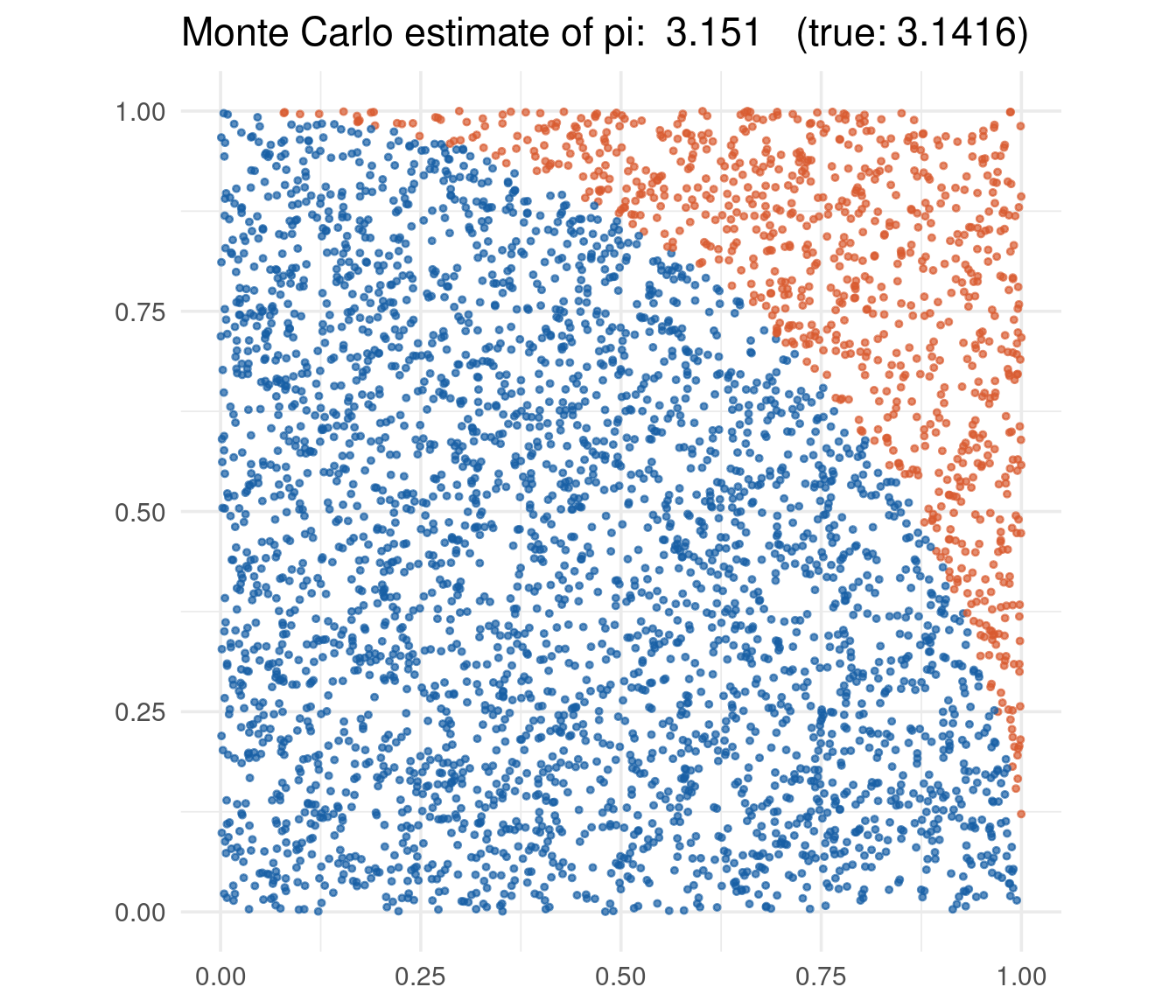

The target is deterministic; the method is stochastic — randomness as a computational tool, not a feature of reality.
Accuracy improves as \(1/\sqrt{N}\): quadruple the points to halve the error.
This is the conceptual core of all Monte Carlo methods in econometrics: bootstrap, Bayesian MCMC, simulated method of moments.

The Huff model: stochastic model, stochastic system

Which shopping mall will a consumer at location \(i\) visit? Genuinely random behavior — so the model predicts probabilities, not choices:

\[ P_{ij} \;=\; \frac{\dfrac{S_j}{T_{ij}^{\lambda}}} {\displaystyle\sum_{k=1}^{n} \dfrac{S_k}{T_{ik}^{\lambda}}} \]

\(S_j\) — attractiveness (size) of mall \(j\)
\(T_{ij}\) — travel time from consumer \(i\) to mall \(j\)
\(\lambda\) — distance-decay parameter (estimated from data)

Huff (1964), doi:10.1177/002224296402800307 — still used daily in retail site selection, and a direct ancestor of the multinomial logit discrete-choice models of McFadden (Nobel 2000).

The Model-Building Process

οἳ λέγομεν ἐν τῶν δημιουργῶν τοιαδί·

we say things like this among the craftsmen

Ἀριστοφάνης, Λυσιστράτη 407

The modelling cycle

\[ \text{Problem} \rightarrow \text{Conceptualize} \rightarrow \text{Specify} \rightarrow \text{Estimate/Calibrate} \rightarrow \text{Validate} \rightarrow \text{Use} \rightarrow \text{Revise} \]

1–2
3–4
5–7

Step 1 — Define the problem. What decision or understanding is the model for? A model without a question is decoration.

Step 2 — Conceptualize. Choose the boundary of the system:

Which variables are endogenous (explained by the model)?
Which are exogenous (taken as given)?
Which mechanisms are first-order and which can be safely ignored?

This is analysis: decomposing the system into elements and relations. The reverse — assembling known elements into a designed system — is synthesis.

Step 3 — Specify. Write the mathematical form: functional forms, equilibrium conditions, stochastic assumptions.

\[ y_i = \beta_0 + \beta_1 x_i + \varepsilon_i, \qquad \varepsilon_i \sim \text{iid}(0, \sigma^2) \]

Step 4 — Estimate or calibrate.

Estimation: let the data choose the parameters (OLS, MLE, GMM)
Calibration: set parameters to match known facts or external studies (standard in DSGE and CGE modelling)

Step 5 — Validate. Confront the model with data it has not seen:

in-sample fit is cheap; out-of-sample performance is the real test
specification tests, residual diagnostics, sensitivity analysis

Step 6 — Use. Prediction, policy analysis, optimization — staying inside the model’s domain of validity.

Step 7 — Revise. Every model eventually breaks. Its failures are data for the next iteration — this loop is scientific progress.

Verification vs validation

Practical rules of thumb for model builders:

Start with the simplest model that could possibly answer the question; add complexity only when the simple model demonstrably fails.
Prefer models whose failures are detectable — a model that cannot be wrong cannot be informative.
Document every assumption; the assumption you did not write down is the one that will break.
Keep a holdout: data, episodes, or facts the model never touched during construction.
Remember Goodhart: the moment your model drives decisions, the system starts adapting to it.

The DGP: a modelling concept at the heart of this course

In econometrics we formalize “the system” as a Data Generating Process:

\[ y_i = f(x_i; \theta) + \varepsilon_i \]

The DGP is the (unknown) mechanism nature uses to produce the data.
An econometric model is our approximation of the DGP.
In simulation studies we invert the game: we play nature, choose \(\theta\), generate data, and check whether our estimators recover the truth.

This is why every deck in this course starts with a DGP: knowing the truth lets us audit our methods. It is the modelling cycle run in a laboratory where, for once, we know the right answer.

A Short History of Economic Models

θήκας τε προγόνων· νῦν ὑπὲρ πάντων ἀγών.

and the tombs of our ancestors — now the struggle is for everything

Αἰσχύλος, Πέρσαι 405

Timeline: 1758–1944

1758
1838–1890
1936–1949
1930s–40s

Quesnay’s Tableau Économique — arguably the first economic model ever.

François Quesnay, physician at Versailles, depicted the economy as circular flow between farmers, landlords, and artisans — inspired by the circulation of blood.
A zig-zag table tracing how expenditure propagates through classes.
Direct ancestor of Leontief’s input–output tables and of modern national accounts.

From Cournot to Marshall — economics becomes mathematical.

Cournot (1838): first use of calculus for economics — duopoly, demand functions, monopoly pricing.
Walras (1874): general equilibrium — all markets clear simultaneously, a system of equations for an entire economy.
Marshall (1890): the supply–demand cross, elasticity, partial equilibrium — the toolkit still taught first today.

Keynes, Hicks, and a hydraulic computer.

Keynes (1936): The General Theory — verbal, revolutionary, ambiguous.
Hicks (1937): compressed Keynes into the IS–LM diagram (doi:10.2307/1907242) — a model of a book.
Phillips (1949): built the MONIAC — a physical hydraulic machine where colored water flowing through tanks simulated national income. A computational model before computers.

Econometrics is born.

Tinbergen (1936–39): first macroeconometric models (Netherlands, then the US for the League of Nations) — dozens of estimated equations. First Nobel in economics (1969, with Frisch).
Cowles Commission (1940s): identification, simultaneous equations — the mathematical foundations of structural econometrics.
Leontief (1936): input–output analysis, doi:10.2307/1927837 — Quesnay’s vision made operational (Nobel 1973).

Timeline: 1944–today

1944–56
1958–76
1980s–now

von Neumann & Morgenstern (1944): Theory of Games and Economic Behavior — strategic interaction becomes mathematics.
Nash (1950): equilibrium for non-cooperative games, doi:10.1073/pnas.36.1.48.
Dantzig (1947): the simplex algorithm — linear programming turns optimization into an industrial tool (Kantorovich had the theory in 1939, in the USSR).
Markowitz (1952): portfolio selection, doi:10.1111/j.1540-6261.1952.tb01525.x — risk becomes a variance.
Solow (1956): the growth model, doi:10.2307/1884513.

Phillips (1958): the inflation–unemployment trade-off, doi:10.1111/j.1468-0335.1958.tb00003.x.
Large Keynesian models (Klein, FRB-MIT-Penn): hundreds of equations, used for actual policy.
Black & Scholes (1973), Merton: option pricing, doi:10.1086/260062.
1970s stagflation: high inflation and high unemployment — the Phillips trade-off collapses in real time.
Lucas (1976): explains why it collapsed — the critique that reshaped macro.

Kydland & Prescott (1982): RBC models — macro rebuilt from optimizing agents; calibration replaces estimation.
1990s–2000s: DSGE models with frictions (New Keynesian) become the central-bank standard.
Engle & Granger (1987): cointegration — modelling non-stationary economic time series honestly.
2000s–now: agent-based models, machine learning, causal inference (natural experiments, diff-in-diff, RDD) — the “credibility revolution”.

Models that failed — and what the failures taught us

Phillips curve
LTCM 1998
2008
Progress

The failure. Policymakers in the 1960s treated the Phillips correlation as a stable menu: “buy” lower unemployment with a little more inflation. In the 1970s both rose together — stagflation.

The lesson. A correlation is not a structure. Agents’ expectations adapt to policy (Friedman, Phelps, Lucas). The failure produced rational expectations, credibility theory, and ultimately independent inflation-targeting central banks — arguably the most successful macro-institutional reform of the century.

The failure. Long-Term Capital Management — a hedge fund with two Nobel laureates (Scholes, Merton) on its board — leveraged convergence trades based on models estimated on recent data. The 1998 Russian default produced correlations and spreads the models deemed essentially impossible. The Fed had to orchestrate a 3.6 billion USD rescue.

The lesson. Fat tails are real; historical covariances break precisely in crises; leverage turns model error into insolvency. Risk management shifted toward stress testing and scenario analysis.

The failure. The Gaussian copula (Li 2000, doi:10.3905/jfi.2000.319253) priced CDOs by assuming a single constant correlation of mortgage defaults, calibrated to a period with no national house-price decline. When prices fell nationwide, defaults clustered far beyond what the model allowed.

The lesson. Validation data must include the stress scenario; tail dependence matters (hence the copula methods deck in this course); a verified model can be invalid; and model risk is now itself a regulated quantity (Basel, CCAR).

Model failures are how the field advances:

Phillips collapse → rational expectations, central-bank independence
LTCM → stress testing, fat-tailed risk models
2008 → macroprudential regulation, tail-dependence modelling, renewed interest in agent-based and behavioral models
Failed forecasts → forecast evaluation literature (Diebold–Mariano), forecast combination, humility

\[ \text{In economics, a well-documented failure is worth more than a lucky forecast.} \]

Mathematical vs Computational Models

ἐς ἄπορον ἥκεις· δεῖ δὲ μηχανῆς τινος.

you have come to an impasse — some contrivance is needed

Εὐριπίδης, Ἑλένη 813

Two ways to extract answers from a model

Analytical
Computational
Compare
Similarities

A mathematical (analytical) model is solved in closed form:

\[ q^* : \; -3q + 17 = 2q + 7 \;\;\Longrightarrow\;\; q^* = 2, \;\; p^* = 11 \]

The answer is a formula — exact, transparent, valid for all parameter values at once.
Comparative statics come free: \(\partial q^*/\partial \text{(demand shift)}\) is readable from the solution.
Price of admission: the model must stay simple enough to solve — linearity, representative agents, convenient functional forms.

A computational model is solved numerically, case by case:

fix parameter values → let the computer iterate/simulate → read the output
handles heterogeneity, non-linearity, frictions, discreteness that kill closed forms
the answer is a number (or a distribution), valid only for the parameters tried
comparative statics require re-running over a grid — and interactions may be missed

	Mathematical	Computational
Solution	closed-form formula	numerical output
Generality	all parameters at once	one parameter point per run
Complexity handled	low–moderate	high
Transparency	full — every step checkable	partial — code is the proof
Errors	algebra mistakes	bugs, discretization, convergence
Typical output	theorem	table / figure / distribution

The two are complements, not rivals:

both start from the same formal specification — assumptions, equations, parameters
both are subject to the same validation duty
analytical results verify code (limiting cases, known special cases)
computation explores where algebra cannot reach, and suggests theorems to prove
modern practice interleaves them: prove what you can, compute the rest

Example: analytical vs computational on the same model

The market model \(p^D = -3q + 17\), \(p^S = 2q + 7\) — solved both ways:

Reading

Code

q <- seq(0, 5, by = 0.01)
df <- tibble(q = q, demand = -3 * q + 17, supply = 2 * q + 7)

# computational solution: grid search for minimal gap
gap  <- abs(df$demand - df$supply)
qhat <- df$q[which.min(gap)]

ggplot(df, aes(q)) +
  geom_line(aes(y = demand), color = "#185FA5", linewidth = 1.4) +
  geom_line(aes(y = supply), color = "#D85A30", linewidth = 1.4) +
  geom_vline(xintercept = qhat, linetype = "dashed", color = "#1D9E75") +
  geom_point(aes(x = 2, y = 11), color = "#1D9E75", size = 4) +
  annotate("text", x = 4.4, y = 6,  label = "demand", color = "#185FA5", size = 5) +
  annotate("text", x = 4.4, y = 16.5, label = "supply", color = "#D85A30", size = 5) +
  annotate("text", x = 2.65, y = 12, label = "q* = 2,  p* = 11", color = "#1D9E75", size = 5) +
  labs(title = "Market equilibrium: analytical point, computational grid search",
       x = "quantity q", y = "price p") +
  theme_minimal(base_size = 14)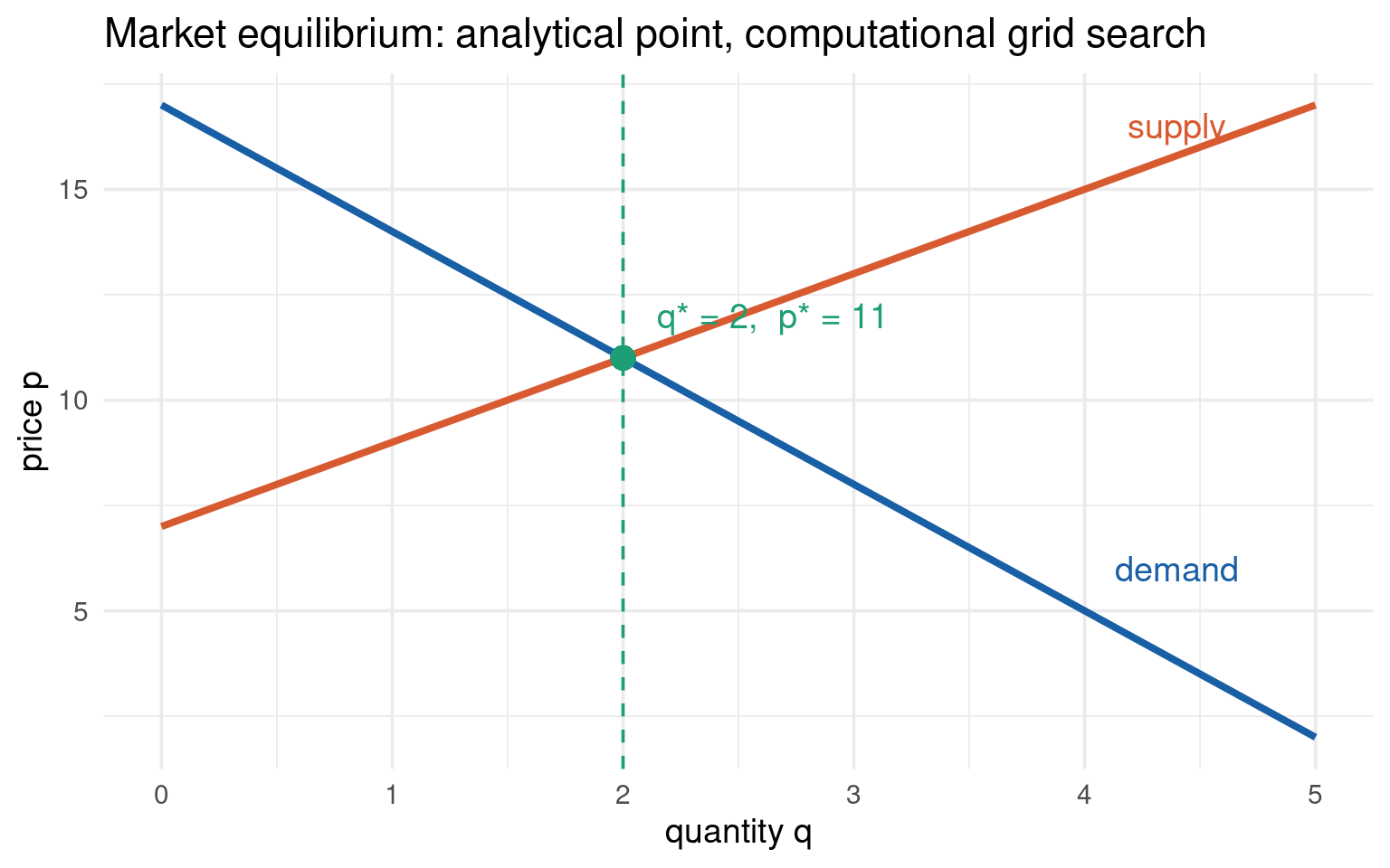

The analytical route sets \(-3q+17 = 2q+7\) and solves: \(q^\ast = 2\), \(p^\ast = 11\) — exact, and instantly tells us how \(q^\ast\) moves if any coefficient changes.
The computational route evaluates both curves on a grid and picks the smallest gap — trivially generalizable to demand curves with no closed form (kinks, empirical demand estimated by ML, stochastic supply).
On a linear model computation is overkill. The point: the same recipe still works when the model becomes non-linear, stochastic, and high-dimensional — where algebra gives up.

The Solow model: dynamics you can see

\[ \Delta k_t = s\,k_t^{\,a} - (\delta + n)\,k_t \qquad\qquad k^\ast = \left( \frac{s}{\delta + n} \right)^{\frac{1}{1-a}} \]

Reading

Code

a <- 0.33; s <- 0.25; delta <- 0.05; n <- 0.01
k_star <- (s / (delta + n))^(1 / (1 - a))

# simulate two economies from different starting points
T <- 80
k_low <- numeric(T); k_high <- numeric(T)
k_low[1] <- 1; k_high[1] <- 25
for (t in 1:(T - 1)) {
  k_low[t + 1]  <- k_low[t]  + s * k_low[t]^a  - (delta + n) * k_low[t]
  k_high[t + 1] <- k_high[t] + s * k_high[t]^a - (delta + n) * k_high[t]
}
df <- tibble(t = 1:T, poor = k_low, rich = k_high) |>
  pivot_longer(-t, names_to = "economy", values_to = "k")

ggplot(df, aes(t, k, color = economy)) +
  geom_line(linewidth = 1.4) +
  geom_hline(yintercept = k_star, linetype = "dashed", color = "#1D9E75", linewidth = 1) +
  annotate("text", x = 70, y = k_star + 1.2, label = "steady state k*",
           color = "#1D9E75", size = 5) +
  scale_color_manual(values = c(poor = "#185FA5", rich = "#D85A30")) +
  labs(title = "Solow convergence: two economies, one destination",
       x = "time", y = "capital per worker k") +
  theme_minimal(base_size = 14) +
  theme(legend.position = "top")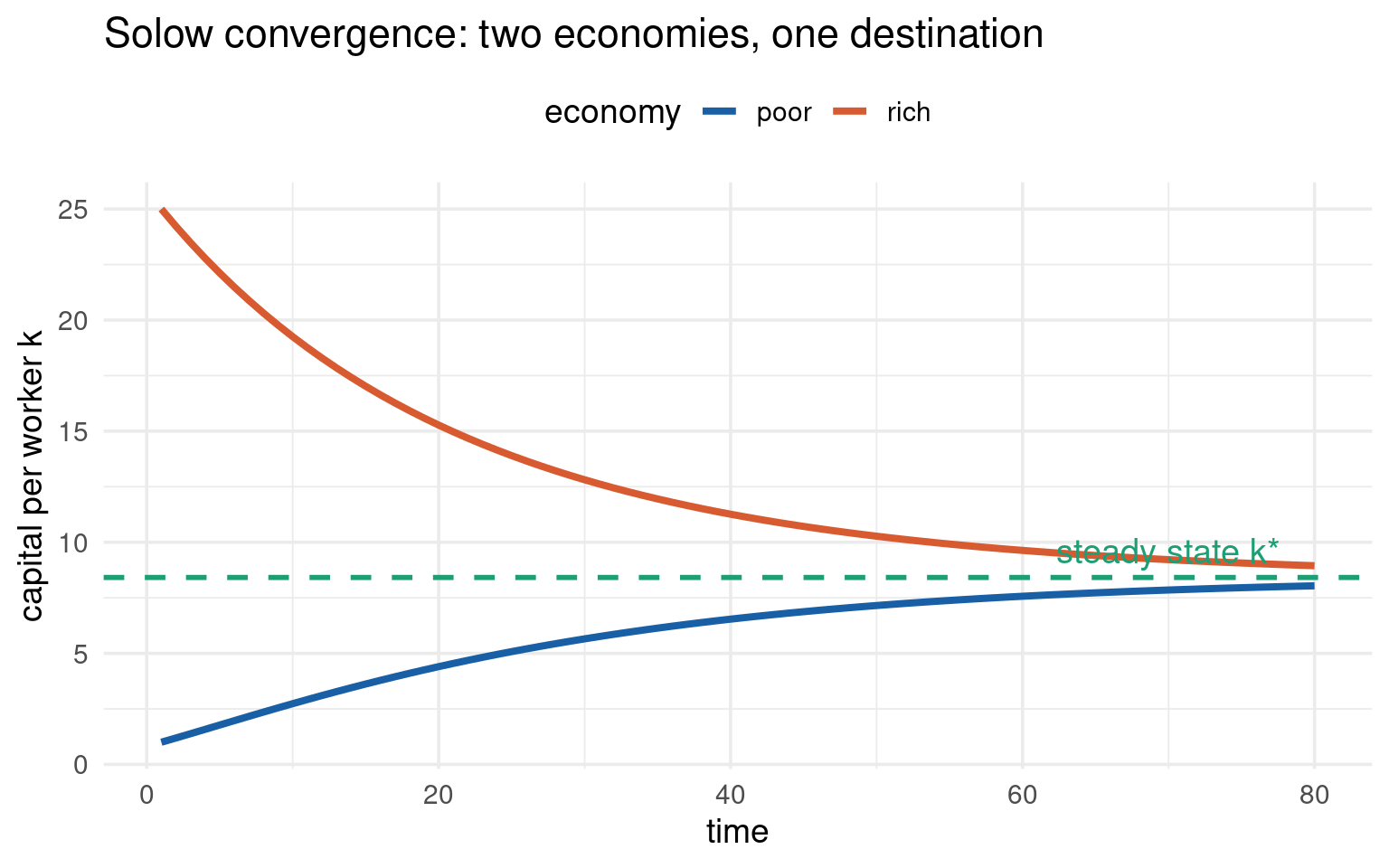

The steady state \(k^\ast\) is an analytical result — one line of algebra.
The transition paths are computational — a simple loop iterating the difference equation.
The model’s big empirical prediction — conditional convergence (poor economies grow faster, given \(s\), \(n\), \(\delta\)) — is visible immediately: the blue economy grows steeply, the red one shrinks toward \(k^\ast\).
This division of labor (algebra for the destination, simulation for the journey) is the standard pattern of modern macro.

Simulation and Optimization

αὐτόματα πάντʼ ἀγαθὰ τῷδέ γε πορίζεται.

every good thing is provided to this man of its own accord

Ἀριστοφάνης, Ἀχαρνῆς 976

What we do with a model, part I: simulation

Simulation = running the model forward under chosen conditions to observe behavior we cannot (or should not) observe in reality.

Types
In business
In economics

Monte Carlo simulation — repeat a stochastic experiment thousands of times; study the distribution of outcomes (bootstrap, risk analysis, power studies)
Discrete-event simulation — entities move through processes with queues (banks, call centers, supply chains, hospitals)
System dynamics — stocks and flows in continuous time (Solow transition, inventory cycles, epidemics)
Agent-based models — many heterogeneous agents with simple rules; aggregate behavior emerges (financial contagion, housing markets, segregation à la Schelling)

A supermarket simulates checkout queues before deciding how many cashiers to hire.
An airline simulates no-show distributions to set overbooking policy.
A factory simulates the production line to find the bottleneck before buying machines.
A bank simulates loan-portfolio losses under stress scenarios (regulatory requirement since 2008).

Central banks simulate DSGE models to trace the effect of an interest-rate move.
Econometricians simulate DGPs to study estimator behavior in finite samples — this course’s daily bread.
Climate–economy models (Nordhaus, Nobel 2018) simulate centuries of interaction between GDP and temperature.
Pension agencies simulate demographic scenarios 50 years ahead.

What we do with a model, part II: optimization

Optimization = finding the decision that makes the model’s objective as good as possible:

\[ \max_{x \in X} \; f(x; \theta) \qquad \text{subject to} \qquad g(x) \le 0 \]

Analytical optimization: first-order conditions, Lagrange multipliers — when \(f\) is smooth and simple
Linear programming: linear objective + linear constraints (Dantzig’s simplex; logistics, blending, scheduling)
Dynamic programming: decisions over time (Bellman); consumption–saving, inventory, option exercise
Stochastic / robust optimization: optimize against uncertainty in \(\theta\) — the Lim (2013) retailer model
Heuristics: genetic algorithms, simulated annealing — when the landscape is non-convex and gradients are useless

Simulation asks “what happens if…?” — optimization asks “what is the best…?”. In practice they combine: simulation–optimization searches for the decision whose simulated outcome distribution is best.

A one-line optimization, visualized

A monopolist with demand \(p = 20 - q\) and cost \(C(q) = 4q + 0.5\,q^2\) maximizes profit:

\[ \pi(q) = (20 - q)\,q - 4q - 0.5\,q^2 \qquad\Longrightarrow\qquad \pi'(q) = 16 - 3q = 0 \;\Longrightarrow\; q^\ast = \tfrac{16}{3} \]

Reading

Code

profit <- function(q) (20 - q) * q - 4 * q - 0.5 * q^2
q  <- seq(0, 10, by = 0.05)

# computational route: R's built-in optimizer
opt <- optimize(profit, interval = c(0, 10), maximum = TRUE)

ggplot(tibble(q = q, pi = profit(q)), aes(q, pi)) +
  geom_line(color = "#185FA5", linewidth = 1.4) +
  geom_vline(xintercept = opt$maximum, linetype = "dashed", color = "#D85A30") +
  geom_point(aes(x = opt$maximum, y = opt$objective), color = "#D85A30", size = 4) +
  annotate("text", x = opt$maximum + 1.9, y = opt$objective,
           label = paste0("q* = ", round(opt$maximum, 3), "  (exact: 16/3)"),
           color = "#D85A30", size = 5) +
  labs(title = "Profit maximization: calculus and optimize() agree",
       x = "quantity q", y = "profit") +
  theme_minimal(base_size = 14)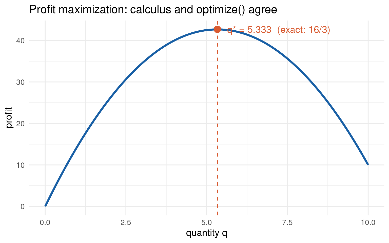

Calculus gives the exact answer \(q^\ast = 16/3 \approx 5.333\) in two lines.
optimize() gives the numerical answer without ever differentiating — and would keep working if \(\pi(q)\) contained a simulation, a kink, or an estimated demand curve.
Agreement between the two routes is the simplest example of verification: analytics checking code, code checking analytics.

The Twelve Most Used Models

τοῦ δώδεκα μνᾶς Πασίᾳ; τί ἐχρησάμην;

twelve minas to Pasias? what did I want it for?

Ἀριστοφάνης, Νεφέλαι 22

The top twelve, at a glance

#	Model	Domain	Key names
1	Supply & demand	Markets	Marshall 1890
2	Linear regression / OLS	Everywhere	Legendre, Gauss; econometrics
3	Cobb–Douglas production	Firms, growth	Cobb & Douglas 1928
4	Solow growth	Macro	Solow 1956
5	IS–LM	Macro policy	Hicks 1937
6	Nash equilibrium / game theory	Strategy	Nash 1950
7	Markowitz portfolio + CAPM	Finance	Markowitz 1952; Sharpe 1964
8	Black–Scholes	Derivatives	Black, Scholes, Merton 1973
9	Discrete choice (logit / Huff)	Marketing, transport	Huff 1964; McFadden 1974
10	Gravity model of trade	International trade	Tinbergen 1962
11	Input–output	National accounts	Leontief 1936
12	Linear programming	Operations	Kantorovich 1939; Dantzig 1947

The next slides give each model one line of math and one line of why it earns its place.

Models 1–4: the market and the firm

Supply & demand.

\[ q^D(p) = q^S(p) \;\;\Longrightarrow\;\; p^\ast \]

The first model every student meets and the last one any economist abandons. Explains prices, taxes, subsidies, price controls, incidence. Its power is its portability: labor markets, housing, foreign exchange — one diagram fits all.

Linear regression (OLS).

\[ y_i = \beta_0 + \beta_1 x_{1i} + \cdots + \beta_k x_{ki} + \varepsilon_i \]

The workhorse of all empirical economics and business analytics. Everything in this course — IV, panel, diff-in-diff, VAR — is regression with extra structure. The most-run model on Earth, by many orders of magnitude.

Cobb–Douglas production function.

\[ Y = A\,K^{a}\,L^{1-a} \]

One equation capturing substitution between capital and labor, constant returns, and factor shares (\(a \approx 1/3\) matches the data remarkably well). Ubiquitous in growth theory, firm-level productivity studies, and CGE models.

Solow growth model.

\[ \Delta k = s\,k^{a} - (\delta + n)\,k \]

The organizing framework for why nations are rich or poor. Its famous residual — the part of growth not explained by capital and labor — redirected the whole field toward technology and human capital. Nobel 1987.

Models 5–8: strategy and finance

IS–LM.

\[ \text{IS: } Y = C(Y - T) + I(r) + G \qquad \text{LM: } \frac{M}{P} = L(Y, r) \]

Hicks’ compression of Keynes into two curves. Criticized for decades, buried repeatedly — yet still how policymakers, journalists, and undergraduates actually reason about fiscal vs monetary policy. A model’s usefulness can outlive its theoretical respectability.

Nash equilibrium.

\[ u_i(s_i^\ast, s_{-i}^\ast) \;\ge\; u_i(s_i, s_{-i}^\ast) \quad \forall\, s_i,\; \forall\, i \]

No player gains by deviating alone. The foundation of modern industrial organization, auction design (spectrum auctions raised billions), contract theory, and market design (Nobel prizes 1994, 2007, 2012, 2020).

Markowitz portfolio + CAPM.

\[ \min_w \; w'\Sigma w \;\; \text{s.t.}\;\; w'\mu = \bar{r} \qquad\qquad E[r_i] = r_f + \beta_i\,(E[r_m] - r_f) \]

Risk became a variance; diversification became mathematics. CAPM’s \(\beta\) is still the default cost-of-capital tool in corporate finance, decades after its empirical troubles were documented.

Black–Scholes.

\[ C = S\,\Phi(d_1) - K e^{-rT}\,\Phi(d_2) \]

The formula that created modern derivatives markets — a rare case of a model performing reality into existence: traders quote prices in its units (implied volatility). Also the origin of one of the great model-risk lessons (1987 crash, volatility smile).

Models 9–12: choice, trade, and operations

Discrete choice: Huff and logit.

\[ P_{ij} = \frac{S_j / T_{ij}^{\lambda}}{\sum_k S_k / T_{ik}^{\lambda}} \qquad\qquad P_{ij} = \frac{e^{x_{ij}'\beta}}{\sum_k e^{x_{ik}'\beta}} \]

From “which mall?” to “which brand, which mode of transport, which job offer?”. McFadden’s conditional logit (Nobel 2000) generalizes Huff’s gravity intuition — the backbone of marketing analytics and transport planning.

Gravity model of trade.

\[ X_{ij} = G\,\frac{Y_i^{\alpha}\, Y_j^{\beta}}{D_{ij}^{\gamma}} \]

Trade between countries \(\sim\) product of their GDPs over distance — Newton’s law transplanted into economics (Tinbergen 1962). The most empirically successful model in international economics: it fits everywhere, always, and now has rigorous micro-foundations.

Input–output (Leontief).

\[ x = A\,x + d \;\;\Longrightarrow\;\; x = (I - A)^{-1} d \]

The economy as a matrix: each sector’s output is others’ input. Quesnay’s Tableau made operational. Used daily for national accounts, supply-chain stress tests, carbon-footprint accounting, and “economic impact” studies.

Linear programming.

\[ \max_x \; c'x \quad \text{s.t.} \quad Ax \le b, \;\; x \ge 0 \]

Kantorovich planned Soviet plywood production with it; Dantzig gave it the simplex algorithm; today it schedules airlines, routes delivery fleets, blends refineries, and clears electricity markets. The quiet workhorse of business decision-making.

Common threads across the twelve

Radical simplicity — each fits on one slide; none tries to model everything
One mechanism each — equilibrium, optimization, choice probability, interdependence
Portability — the gravity equation works for trade, migration, phone calls, and shopping trips
Longevity through usefulness — several are “empirically falsified” (CAPM, IS–LM) yet remain in daily use because nothing equally simple answers the question better
Failure-driven refinement — each has a documented breakdown that spawned its successor (Phillips → expectations-augmented; Black–Scholes → smile models; Solow → endogenous growth)

Rodrik again: economics is a library of models, and these twelve are the shelf every economist and business analyst reaches for first.

Exercises

Exercises — Concepts

Give one example (not from these slides) of each cell of the 2×2 taxonomy: deterministic/stochastic model of a deterministic/stochastic system. Justify each classification.
Take the metro-map analogy. Identify three ways in which a national accounts table (GDP statistics) is “geographically wrong” about the economy, yet useful — and one question for which it is the wrong map.
Friedman vs Samuelson: state the F-twist in one sentence, state the strongest objection to it in one sentence, and give a 2008-crisis example supporting the objection.
Explain the difference between verification and validation using the Gaussian-copula CDO model as the example.
State the Lucas critique in your own words and give a business (not macro) example: a company exploits a historical pattern in customer behavior, and the pattern collapses because of the exploitation.
For the Kennedy/Clinton contrast, propose a third “presidential challenge” from economics (e.g., “eliminate inflation”, “end unemployment”) and argue whether it is Moon-like or vaccine-like — that is, whether the binding constraint is engineering or a missing model.

Exercises — Models

Solve the market model \(p^D = -3q + 17\), \(p^S = 2q + 7\) after a per-unit tax \(t = 2.5\) is imposed on sellers. Find the new equilibrium analytically, then verify with a grid search in R.
In the Solow simulation, double the savings rate to \(s = 0.50\). Compute the new \(k^\ast\) analytically, re-run the simulation, and describe what changes in the transition and what changes in the destination.
Modify the Monte Carlo \(\pi\) experiment: run it for \(N \in \{10^2, 10^3, 10^4, 10^5\}\) with 100 replications each, and plot the standard deviation of \(\hat{\pi}\) against \(N\) on a log-log scale. Confirm the \(1/\sqrt{N}\) rate.
A city has three malls with sizes \(S = (100, 50, 30)\) and travel times from your home \(T = (10, 5, 4)\) minutes. Compute your Huff probabilities for \(\lambda = 1\) and \(\lambda = 2\). Which mall gains most when \(\lambda\) rises, and why?
The monopolist’s cost changes to \(C(q) = 4q + 0.5q^2 + 15\) (a fixed cost). Show analytically that \(q^\ast\) is unchanged, verify with optimize(), and explain the economic principle involved.
Pick one of the twelve models and write half a page on a documented real-world failure of it, and on what replaced or repaired it.

Models and Modelling in Economics and Business

Required Packages

Literature Review

Outline

Two definitions

Why models? Why not study reality directly?

Two presidential challenges

Open questions for economists

Economists speak with models

All models are wrong

Friedman’s provocation: do assumptions matter?

The map is not the territory

In the beginning: the invisible hand

Models are mathematics

Classifying model activities

System type × model type: the 2×2

Monte Carlo estimation of \(\pi\)

The Huff model: stochastic model, stochastic system

The modelling cycle

Verification vs validation

The DGP: a modelling concept at the heart of this course

Timeline: 1758–1944

Timeline: 1944–today

Models that failed — and what the failures taught us

Two ways to extract answers from a model

Example: analytical vs computational on the same model

The Solow model: dynamics you can see

What we do with a model, part I: simulation

What we do with a model, part II: optimization

A one-line optimization, visualized

The top twelve, at a glance

Models 1–4: the market and the firm

Models 5–8: strategy and finance

Models 9–12: choice, trade, and operations

Common threads across the twelve

Exercises — Concepts

Exercises — Models

Further Reading