Moments-Based Structural Estimation

GMM, Empirical Likelihood, Simulated Moments and Indirect Inference
using R, Python & Stata

Athanassios Stavrakoudis

astavrak@uoi.gr

Applied Informatics and Computational Economics Lab

19 July 2026

Outline

• Roadmap
• How the deck is ordered
• Scope

• Part 1 — From theory to moment conditions
  the analogy principle, identification, asymptotics, the efficient weight
• Part 2 — The GMM machinery
  a known-truth DGP, by hand and off the shelf, \(S\) and the estimator zoo
• Part 3 — Overidentification & finite samples
  the \(J\) and \(C\) tests, CUE, empirical likelihood, implied probabilities
• Part 4 — Simulation-based moments
  SMM, indirect inference, EMM, common random numbers

• Part 5 — Real data I: the Euler equation
  Hansen–Singleton on 1948–2026, weak identification, HAC choice
• Part 6 — Real data II: the SDF
  Fama–French portfolios, Hansen–Jagannathan, sensitivity to moments
• Part 7 — Real data III & IV
  stochastic volatility by II/SMM; dynamic panels on EU regions
• Part 8 — Modern practice
  misspecification, moment selection, bootstrap, computation, exercises, reading

One object runs through every slide:

\[\mathbb{E}\big[g(w_i, \theta_0)\big] = 0\]

Parts 1–4 build the machinery on data whose truth we know, so every estimate can be checked against a number. Parts 5–7 turn the same code on real data, where no truth exists and the diagnostics are all we have. Part 8 is what to do when the diagnostics say the model is wrong.

Two departures from the standard order in this series, both deliberate:

1. The tests are distributed, not collected. The \(J\) test belongs beside the DGP that motivates it (Part 3), the weak-identification tests beside the Euler equation that suffers from them (Part 5), the AR(2) and Hansen tests beside the dynamic panel (Part 7). Each still gets its own theory slide and code slide.

2. There are four applications, not one. Moment conditions come from very different economics — an Euler equation, a stochastic discount factor, a volatility process, a dynamic panel — and the point is that the same estimator handles all four.

This deck is about the estimator family, not the model catalogue.

Two companion decks cover the models. Structural Estimation in Econometrics owns Cowles simultaneity, Rust’s bus engine (NFXP and CCP), BLP demand, production functions, entry games, auctions and equilibrium search. Advanced Structural Econometrics owns dynamic games, auction theory and HANK. None of that is repeated here.

Those decks ask which structural model describes this market?
This deck asks given the moment conditions a model implies, how do I estimate, test and defend the parameters — and what do I do when the overidentification test rejects?

The overlap is honest and small: GMM, SMM and indirect inference appear in the structural deck across six slides on simulated toy data. Here they get thirty, on data with a 2026 vintage.

Required Packages

library(gmm)          # gmm(), gel() — two-step, iterated, CUE, EL, ET, CUE-GEL
library(momentfit)    # momentModel(), gmmFit(), gelFit(), specTest() — modern API
library(sandwich)     # vcovHAC(), kweights(), bwAndrews() — weighting matrices
library(numDeriv)     # jacobian(), grad() — numerical G when analytic is painful
library(plm)          # pgmm() — Arellano-Bond, Blundell-Bond system GMM
library(AER)          # ivreg() — the 2SLS benchmark GMM should reproduce
library(quantmod)     # getSymbols() — used by moments-data.R, not by the deck
library(eurostat)     # get_eurostat() — likewise
library(tidyverse)    # wrangling & ggplot2
library(png)          # readPNG() — reload Stata-exported graphs

import numpy as np                      # arrays, linear algebra
import pandas as pd                     # data frames, CSV input
import scipy.stats as st                # distributions
from scipy.optimize import minimize     # every hand-coded criterion
from linearmodels.iv import IVGMM, IVGMMCUE          # linear GMM, CUE
from statsmodels.sandbox.regression.gmm import GMM   # subclass for nonlinear moments
import statsmodels.api as sm            # HAC covariance, ACF
from arch import arch_model             # GARCH auxiliary model for indirect inference
import numdifftools as nd               # Jacobians of the moment vector
from joblib import Parallel, delayed    # parallel Monte Carlo
import matplotlib.pyplot as plt         # all figures

* Ships with Stata SE — no installation needed:
gmm              // the general estimator: linear, nonlinear, interactive, moment-evaluator
ivregress gmm    // linear IV by GMM, one-step / two-step / iterated
estat overid     // Hansen J after ivregress
xtabond xtdpdsys // Arellano-Bond and Blundell-Bond, native versions
mata: optimize() // SMM, indirect inference and empirical likelihood are written here

* From SSC:
ssc install ivreg2       // ivreg2 + weak-identification statistics
ssc install ranktest     // Kleibergen-Paap rank test (required by ivreg2)
ssc install xtabond2     // Roodman's system GMM, with proper instrument accounting
ssc install estout       // esttab result tables

Stata has no native empirical likelihood, no native SMM and no native indirect inference. Where a slide needs one it is hand-coded in Mata with optimize(), and the tab says so rather than quietly disappearing.

Data & Provenance

Every dataset is written once by moments-data.R and only read by the deck. Downloads are cached in ../data/moments-raw-*.csv, so a rendered deck is reproducible offline and its numbers do not move when a provider restates history.

File	Span	Content	Source
moments-dgp.csv	\(n = 2000\)	Structural demand with an exponential mean, known \(\beta\); strong- and weak-instrument variants	simulated, seed 14159
moments-latent.csv	\(T = 2000\)	Stochastic volatility with known \((\mu, \phi, \sigma_\eta)\)	simulated, seed 14159
moments-ccapm.csv	1948Q2–2026Q1	Real per-capita consumption growth, gross real risk-free and market returns	FRED + Ken French
moments-ff.csv	1963-07–2026-05	Mkt-RF, SMB, HML, RF + 25 size/BM portfolio excess returns	Ken French Data Library
moments-spx.csv	2006–2026	Daily S&P 500 log returns	Yahoo Finance
moments-panel.csv	2000–2024	266 EU NUTS-2 regions: real GDP per head (PPS) and growth	Eurostat nama_10r_2gdp

Vintages are stated, not implied. The Ken French files come from the CRSP 202605 vintage; both providers revise history, and Yahoo’s adjusted closes are restated for dividends and splits. The deck reads the cached raw files, so the numbers on these slides are fixed. It is the re-download that is not bit-identical, not the render.

Part 1 — From Theory to Moment Conditions

The Problem — What Are You Willing to Assume?

• Two Contracts
• The Bargain
• Where This Deck Goes

Maximum likelihood asks you to write down the entire distribution of the data:

\[\mathcal{L}(\theta) = \prod_{i=1}^{n} f(w_i \mid \theta)\]

In exchange it gives the smallest asymptotic variance any consistent estimator can have. The price is that every piece of \(f\) must be right. Get the error distribution wrong and the estimator is not merely inefficient — it is inconsistent.

The method of moments asks for much less: a finite list of things the model says should average to zero.

\[\mathbb{E}\big[g(w_i, \theta_0)\big] = 0\]

Nothing else about the distribution is specified. No density, no error term, no closed-form likelihood.

	Maximum likelihood	Method of moments
You supply	the full density \(f(w \mid \theta)\)	a vector of moment conditions
You get	the efficiency bound	\(\sqrt{n}\)-consistency, asymptotic normality
It breaks when	any part of \(f\) is misspecified	the moments themselves are wrong
Needs a tractable likelihood	yes	no

That last row is why this deck exists. Enormous classes of structural models — dynamic discrete choice, equilibrium games, stochastic volatility, anything with a latent state integrated out — have a likelihood that cannot be written down or cannot be computed. They all deliver moment conditions.

Four applications, four sources of moments, one estimator:

• a household’s Euler equation — Part 5
• an asset-pricing stochastic discount factor — Part 6
• a latent volatility process with no likelihood — Part 7
• a dynamic panel where the fixed effect must be differenced away — Part 7

Is ML really more efficient? Only if it is right

The efficiency claim is conditional on correct specification. Two qualifications matter in practice.

1. The score is a moment condition. ML is a special case of the method of moments, with

\[ g(w_i, \theta) = \frac{\partial \log f(w_i \mid \theta)}{\partial \theta} \]

because the score has mean zero at the truth. So GMM does not compete with ML — it contains it. Choosing GMM means choosing a different, usually shorter, list of moments.

2. Efficiency is not robustness. If \(f\) is misspecified the ML estimator converges to the pseudo-true value that minimises the Kullback–Leibler distance to the truth — which is generally not \(\theta_0\). A GMM estimator built on moments that survive the misspecification stays consistent. The relevant comparison is therefore not “which has the smaller variance?” but “which assumptions am I prepared to defend?”

Part 3 makes this concrete: the \(J\) test asks whether the moments you chose are mutually consistent, and Part 8 asks what your standard errors mean once you concede they are not.

The Analogy Principle

The oldest idea in estimation: if the population satisfies an equality, impose the same equality on the sample.

Pearson (1894) matched the first \(k\) raw moments of a mixture of two normals to their sample counterparts and solved the resulting equations:

\[\mathbb{E}\big[w_i^{\,j}\big] = m_j(\theta), \qquad j = 1, \dots, k\]

\[\frac{1}{n}\sum_{i=1}^n w_i^{\,j} = m_j(\hat\theta)\]

Exactly identified. With as many equations as parameters the sample equations can generally be solved exactly, and \(\bar g(\hat\theta) = 0\) holds to machine precision. The weight matrix is irrelevant — there is nothing to trade off.

Over-identified. With more equations than parameters no \(\theta\) sets all of them to zero at once. Something must give, and the whole of GMM is the answer to what:

\[\hat\theta = \arg\min_\theta \ \bar g(\theta)' W \bar g(\theta)\]

Hansen (1982) supplied that answer, together with the asymptotic theory and the specification test that the surplus equations give away for free.

Where Moment Conditions Come From

Economics rarely hands you a density. It routinely hands you an equality that must hold at an optimum or in equilibrium — and that is a moment condition.

• Euler equations
• First-order conditions
• Orthogonality
• Equilibrium conditions
• Binding functions

An optimising household equates the marginal cost of saving a euro today to the discounted marginal benefit tomorrow. With CRRA utility:

\[\mathbb{E}\left[\beta\left(\frac{C_{t+1}}{C_t}\right)^{-\gamma} R_{t+1} - 1 \ \Big|\ \mathcal{I}_t\right] = 0\]

Conditioning on \(\mathcal{I}_t\) is what makes it operational: anything the household knew at \(t\) is a valid instrument, so one theoretical restriction generates as many moments as you have lags. Part 5.

A firm choosing inputs to maximise profit sets the marginal revenue product equal to the factor price. A bidder’s expected-payoff condition, a wage-posting condition, a regulator’s optimality condition — each is an equality in expectation whose sample analogue can be imposed:

\[\mathbb{E}\big[\mathrm{MRP}_i(\theta) - w_i\big] = 0\]

The workhorse. If an instrument is excluded from the structural equation and uncorrelated with its error, that is the moment condition:

\[\mathbb{E}\big[z_i \, u_i(\theta)\big] = 0\]

2SLS, IV and the whole Part 2 DGP are this one line. So is the Arellano–Bond condition that lagged levels are orthogonal to differenced errors — Part 7.

Market clearing, a fixed point, a zero-profit condition. In asset pricing, the statement that one discount factor prices every asset is exactly a moment condition — one per asset:

\[\mathbb{E}\big[m_t(\theta) \, R^e_{jt}\big] = 0, \qquad j = 1, \dots, 25\]

Twenty-five assets, three parameters, twenty-two over-identifying restrictions. Part 6.

When a model can be simulated but not written down, the moments can be statistics of simulated data matched to the same statistics of real data:

\[\mathbb{E}\big[m(w_i)\big] - \frac{1}{S}\sum_{s=1}^{S} m\big(w_i^{s}(\theta)\big) = 0\]

That is the method of simulated moments; taking \(m(\cdot)\) to be the parameters of an auxiliary model gives indirect inference. Parts 4 and 7.

Literature Review

• Origins
• Weighting and inference
• Empirical likelihood and GEL
• Simulation-based
• When it goes wrong

• Pearson (1894) — the method of moments, fitting a mixture of two normals
• Hansen (1982) — GMM: the estimator, its asymptotics and the \(J\) test, in one paper
• Hansen & Singleton (1982) — the first great application: nonlinear rational-expectations Euler equations

• Newey & West (1987) — a HAC estimator guaranteed positive semi-definite
• Andrews (1991) — optimal kernels and automatic bandwidth selection
• Hansen, Heaton & Yaron (1996) — two-step versus iterated versus continuously updated, in finite samples

• Qin & Lawless (1994) — empirical likelihood for general estimating equations
• Imbens (2002) — a readable bridge from GMM to empirical likelihood
• Newey & Smith (2004) — why GEL has smaller higher-order bias than two-step GMM

• McFadden (1989) — the method of simulated moments
• Pakes & Pollard (1989) — asymptotics for non-smooth simulated criteria
• Duffie & Singleton (1993) — simulated moments for Markov models of asset prices
• Gouriéroux, Monfort & Renault (1993) — indirect inference
• Gallant & Tauchen (1996) — the efficient method of moments: which moments to match

• Andrews (1999) — consistent moment selection
• Stock & Wright (2000) — GMM when identification is weak
• Andrews, Gentzkow & Shapiro (2017) — which moments actually move your estimate
• Hansen & Lee (2021) — inference for iterated GMM under misspecification

GMM, Defined

Let \(\theta \in \Theta \subset \mathbb{R}^{k}\) and let \(g(w_i,\theta) \in \mathbb{R}^{q}\) with \(q \geq k\). The population statement that defines the estimand:

\[\mathbb{E}\big[g(w_i, \theta)\big] = 0 \quad \text{ if and only if } \quad \theta = \theta_0\]

Its sample analogue, and the criterion built from it:

\[\bar g(\theta) = \frac{1}{n}\sum_{i=1}^{n} g(w_i, \theta), \qquad Q_n(\theta) = \bar g(\theta)' \, W \, \bar g(\theta)\]

\[\hat\theta = \arg\min_{\theta \in \Theta} \ Q_n(\theta)\]

Symbol	Meaning	In the Part 2 DGP
\(q\)	number of moment conditions	6
\(k\)	number of parameters	3
\(q - k\)	over-identifying restrictions	3
\(W\)	\(q \times q\) weight matrix, positive definite	\(I\), then \(\hat S^{-1}\)
\(G\)	Jacobian \(\mathbb{E}[\partial g_i / \partial\theta']\)	\(6 \times 3\)
\(S\)	long-run variance of \(\sqrt{n}\,\bar g(\theta_0)\)	\(6 \times 6\)

Everything after this slide follows from choosing \(g\), choosing \(W\), and asking what \(\hat\theta\) inherits from those two choices.

Identification — Order and Rank

• The Two Conditions

Order condition — necessary, and merely arithmetic:

\[q \geq k\]

Rank condition — the one that actually bites:

\[\mathrm{rank}(G) = k, \qquad G = \mathbb{E}\left[\frac{\partial g(w_i,\theta_0)}{\partial \theta'}\right]\]

If \(G\) is rank deficient then some direction in parameter space leaves the moments unchanged to first order: the data cannot distinguish \(\theta_0\) from a neighbour, and no sample size repairs it.

Rank is a knife-edge concept, and that is its weakness in practice. In finite samples \(\hat G\) is almost never exactly deficient. What hurts is being close to deficient — a smallest singular value near zero:

\[\sigma_{\min}(G) \to 0 \quad \Longrightarrow \quad \text{standard errors explode and } t\text{-ratios mislead}\]

The code tabs make the point on the Part 2 data: strong and weak instruments both give rank 3, and the two cases are nothing alike.

d <- read.csv("../data/moments-dgp.csv")
n <- nrow(d)
Z <- cbind(1, d$z1, d$z2, d$z3, d$z4, d$x)
b <- c(1.9947, -0.7817, 0.3956)

Gmat <- function(price) {                  # the 6 x 3 Jacobian at b
  mu <- exp(b[1] + b[2]*price + b[3]*d$x)
  -crossprod(Z, cbind(1, price, d$x) * mu) / n
}
G_strong <- Gmat(d$p)
G_weak   <- Gmat(d$p_weak)                 # cost shifters at 6% strength

cat(sprintf("strong : rank %d, singular values %.3f %.3f %.3f\n",
            qr(G_strong)$rank, svd(G_strong)$d[1],
            svd(G_strong)$d[2], svd(G_strong)$d[3]))
cat(sprintf("weak   : rank %d, singular values %.3f %.3f %.3f\n",
            qr(G_weak)$rank, svd(G_weak)$d[1],
            svd(G_weak)$d[2], svd(G_weak)$d[3]))

strong : rank 3, singular values 6.831 3.182 2.000

weak   : rank 3, singular values 6.507 3.037 0.165

Both have full rank 3. The smallest singular value is 12.1 times

larger with strong instruments: rank is not the useful diagnostic.

import numpy as np, pandas as pd

d = pd.read_csv("../data/moments-dgp.csv")
n = len(d)
Z = np.column_stack([np.ones(n), d.z1, d.z2, d.z3, d.z4, d.x])
b = np.array([1.9947, -0.7817, 0.3956])

def Gmat(price):                           # the 6 x 3 Jacobian at b
    mu = np.exp(b[0] + b[1]*price + b[2]*d.x.values)
    return -Z.T @ (np.column_stack([np.ones(n), price, d.x]) * mu[:, None]) / n

G_strong = Gmat(d.p.values)
G_weak   = Gmat(d.p_weak.values)           # cost shifters at 6% strength
sv_s = np.linalg.svd(G_strong, compute_uv = False)
sv_w = np.linalg.svd(G_weak,   compute_uv = False)

out = (f"strong : rank {np.linalg.matrix_rank(G_strong)}, "
       f"singular values {sv_s[0]:.3f} {sv_s[1]:.3f} {sv_s[2]:.3f}\n"
       f"weak   : rank {np.linalg.matrix_rank(G_weak)}, "
       f"singular values {sv_w[0]:.3f} {sv_w[1]:.3f} {sv_w[2]:.3f}\n\n"
       f"Both have full rank 3. The smallest singular value is "
       f"{sv_s[-1]/sv_w[-1]:.1f} times\nlarger with strong instruments: "
       f"rank is not the useful diagnostic.")
import sys; nch = sys.stdout.write(out + "\n"); sys.stdout.flush()

strong : rank 3, singular values 6.831 3.182 2.000
weak   : rank 3, singular values 6.507 3.037 0.165

Both have full rank 3. The smallest singular value is 12.1 times
larger with strong instruments: rank is not the useful diagnostic.

quietly import delimited "../data/moments-dgp.csv", clear
quietly destring _all, replace

mata:
real matrix Gmat(real colvector price, real matrix Z, real colvector xv,
                 real rowvector b, real scalar n) {
    mu = exp(b[1] :+ b[2]*price :+ b[3]*xv)
    return(-quadcross(Z, (J(n,1,1), price, xv) :* mu) / n)
}
xv = st_data(., "x")
n  = rows(xv)
Z  = (J(n,1,1), st_data(., ("z1","z2","z3","z4","x")))
b  = (1.9947, -0.7817, 0.3956)

Gs = Gmat(st_data(., "p"),      Z, xv, b, n)
Gw = Gmat(st_data(., "p_weak"), Z, xv, b, n)     // shifters at 6% strength
ss = svdsv(Gs); sw = svdsv(Gw)

printf("strong : rank %1.0f, singular values %6.3f %6.3f %6.3f\n",
       rank(Gs), ss[1], ss[2], ss[3])
printf("weak   : rank %1.0f, singular values %6.3f %6.3f %6.3f\n",
       rank(Gw), sw[1], sw[2], sw[3])
printf("\nBoth have full rank 3. The smallest singular value is %4.1f times\n",
       ss[3]/sw[3])
printf("larger with strong instruments: rank is not the useful diagnostic.\n")
end

------------------------------------------------- mata (type end to exit) ----------------------------------------------
: real matrix Gmat(real colvector price, real matrix Z, real colvector xv,
>                  real rowvector b, real scalar n) {
>     mu = exp(b[1] :+ b[2]*price :+ b[3]*xv)
>     return(-quadcross(Z, (J(n,1,1), price, xv) :* mu) / n)
> }

: xv = st_data(., "x")

: n  = rows(xv)

: Z  = (J(n,1,1), st_data(., ("z1","z2","z3","z4","x")))

: b  = (1.9947, -0.7817, 0.3956)

: 
: Gs = Gmat(st_data(., "p"),      Z, xv, b, n)

: Gw = Gmat(st_data(., "p_weak"), Z, xv, b, n)     // shifters at 6% strength

: ss = svdsv(Gs); sw = svdsv(Gw)

: 
: printf("strong : rank %1.0f, singular values %6.3f %6.3f %6.3f\n",
>        rank(Gs), ss[1], ss[2], ss[3])
strong : rank 3, singular values  6.831  3.182  2.000

: printf("weak   : rank %1.0f, singular values %6.3f %6.3f %6.3f\n",
>        rank(Gw), sw[1], sw[2], sw[3])
weak   : rank 3, singular values  6.507  3.037  0.165

: printf("\nBoth have full rank 3. The smallest singular value is %4.1f times\n",
>        ss[3]/sw[3])

Both have full rank 3. The smallest singular value is 12.1 times

: printf("larger with strong instruments: rank is not the useful diagnostic.\n")
larger with strong instruments: rank is not the useful diagnostic.

: end
------------------------------------------------------------------------------------------------------------------------

Asymptotics — What \(\hat\theta\) Inherits

Under identification, smoothness and a central limit theorem for the moments,

\[\sqrt{n}\,\bar g(\theta_0) \ \xrightarrow{\ d\ } \ \mathcal{N}(0, S)\]

Expanding the criterion’s first-order condition around \(\theta_0\) transfers that normality to the estimator:

\[\sqrt{n}\big(\hat\theta - \theta_0\big) \ \xrightarrow{\ d\ } \ \mathcal{N}(0, V_W)\]

\[V_W = \big(G'WG\big)^{-1} G'WSWG \big(G'WG\big)^{-1}\]

Three readings of that sandwich, each of which returns later:

• \(V_W\) depends on \(W\), so the weight matrix is not innocuous — it changes precision, though never consistency
• \(G\) enters inverted: as \(G\) approaches rank deficiency \(V_W\) explodes. This is the algebra behind weak identification in Part 5
• \(S\) must be estimated, and how you estimate it is a modelling choice rather than a default — Part 2

The Efficient Weight

Choose \(W\) to make the sandwich as small as possible. For any fixed set of moments the answer is the inverse of their variance:

\[W^{*} = S^{-1} \qquad \Longrightarrow \qquad V^{*} = \big(G' S^{-1} G\big)^{-1}\]

and \(V_W - V^{*}\) is positive semi-definite for every other admissible \(W\). This is the GMM efficiency bound: given these moment conditions, no \(\sqrt{n}\)-consistent estimator does better.

The intuition is inverse-variance weighting. A moment that is noisy, or nearly a linear combination of the others, should not be allowed to push \(\hat\theta\) around as hard as a precise and independent one — and \(S^{-1}\) does exactly that bookkeeping.

Two warnings, both cashed out later:

• \(S^{-1}\) is optimal for the moments you chose. A longer list can do better still, which is why Part 8 asks how to choose moments at all
• \(S\) has to be estimated, and \(\hat S\) is correlated with \(\bar g\). That correlation is the origin of two-step GMM’s finite-sample bias, and the reason CUE and empirical likelihood exist — Part 3

Why \(S^{-1}\) is optimal, in three lines

Write \(S = CC'\) and rescale the moments to \(\tilde g = C^{-1}\bar g\), which has identity variance. In those units the problem is an ordinary projection and the Gauss–Markov logic applies directly.

Formally, for any admissible \(W\) the gap between the two variances is

\[ V_W - V^{*} = A \big( I - P \big) A' \]

where \(A = (G'WG)^{-1}G'WC\) and \(P\) is the orthogonal projection onto the column space of \(C^{-1}G\). Since \(I - P\) is idempotent and positive semi-definite, so is the whole expression, and therefore

\[ V_W \succeq V^{*} = (G'S^{-1}G)^{-1} \]

with equality exactly when \(W \propto S^{-1}\). Note what the argument does not say: it takes the moment function \(g\) as given. Optimality here means optimality within a chosen set of moment conditions, never across different ones — adding a genuinely informative moment lowers the bound itself.

Part 2 — The GMM Machinery

DGP — Mathematical Specification

• The Model
• The Moment Conditions
• Why Not Just Take Logs?

A demand equation with a constant semi-elasticity of quantity to price:

\[q_i = \exp\!\big(\beta_0 + \beta_1 p_i + \beta_2 x_i\big) + u_i\]

Price is not handed down by nature. It is set by four cost shifters and by a supply shock \(v_i\) that also moves demand:

\[p_i = 1 + 0.35 z_{1i} + 0.28 z_{2i} + 0.22 z_{3i} + 0.18 z_{4i} + 0.5 v_i\]

\[\mathrm{corr}(u_i, v_i) = 0.95, \qquad \sigma_u = 1.2\]

The truth, which we keep checking against:

\[\beta_0 = 2.0, \qquad \beta_1 = -0.8, \qquad \beta_2 = 0.4\]

The cost shifters are excluded from demand and \(x_i\) is exogenous, so

\[\mathbb{E}\big[u_i \mid z_i, x_i\big] = 0\]

Six unconditional moments follow, one per instrument:

\[\mathbb{E}\Big[(1, z_{1i}, z_{2i}, z_{3i}, z_{4i}, x_i)' \big(q_i - \exp(\beta_0 + \beta_1 p_i + \beta_2 x_i)\big)\Big] = 0\]

Six moments, three parameters. The model is over-identified with

\[q - k = 6 - 3 = 3 \ \text{ degrees of freedom}\]

Two reasons this cannot be turned into a linear IV problem.

The error is additive, not multiplicative. Logging \(q_i = \exp(\cdot) + u_i\) separates nothing:

\[\log q_i \neq \beta_0 + \beta_1 p_i + \beta_2 x_i + \tilde u_i\]

And the sample settles it — 0.25% of the quantities come out negative, so

\[\log q_i \ \text{ is undefined for } \ 5 \ \text{ observations}\]

The moment conditions never take a log, so they do not care. This is the argument Santos Silva & Tenreyro (2006) make against log-linearising gravity equations.

DGP — Code Implementation

The deck never generates data. moments-data.R wrote ../data/moments-dgp.csv once, with the seed 14159 hard-coded; every tab below only reads it.

d <- read.csv("../data/moments-dgp.csv")

cat(sprintf("n = %d\n", nrow(d)))
cat(sprintf("q : mean %.3f  sd %.3f  min %.2f  max %.2f\n",
            mean(d$q), sd(d$q), min(d$q), max(d$q)))
cat(sprintf("p : mean %.3f  sd %.3f\n", mean(d$p), sd(d$p)))
cat(sprintf("share of q below zero : %.4f\n", mean(d$q < 0)))

first <- lm(p ~ z1 + z2 + z3 + z4, data = d)
cat(sprintf("first-stage F on the four cost shifters : %.1f\n",
            summary(first)$fstatistic[1]))

n = 2000

q : mean 4.319  sd 3.158  min -0.85  max 35.98

p : mean 0.991  sd 0.746

share of q below zero : 0.0025

first-stage F on the four cost shifters : 619.9

import numpy as np, pandas as pd, statsmodels.api as sm

d = pd.read_csv("../data/moments-dgp.csv")
first = sm.OLS(d.p, sm.add_constant(d[["z1", "z2", "z3", "z4"]])).fit()

out = (f"n = {len(d)}\n"
       f"q : mean {d.q.mean():.3f}  sd {d.q.std(ddof=1):.3f}  "
       f"min {d.q.min():.2f}  max {d.q.max():.2f}\n"
       f"p : mean {d.p.mean():.3f}  sd {d.p.std(ddof=1):.3f}\n"
       f"share of q below zero : {(d.q < 0).mean():.4f}\n"
       f"first-stage F on the four cost shifters : {first.fvalue:.1f}")
import sys; nch = sys.stdout.write(out + "\n"); sys.stdout.flush()

n = 2000
q : mean 4.319  sd 3.158  min -0.85  max 35.98
p : mean 0.991  sd 0.746
share of q below zero : 0.0025
first-stage F on the four cost shifters : 619.9

quietly import delimited "../data/moments-dgp.csv", clear
quietly destring _all, replace

summarize q p
quietly count if q < 0
display "share of q below zero : " %6.4f r(N)/_N

quietly regress p z1 z2 z3 z4
display "first-stage F on the four cost shifters : " %6.1f e(F)

    Variable |        Obs        Mean    Std. dev.       Min        Max
-------------+---------------------------------------------------------
           q |      2,000    4.319423    3.157538  -.8466021   35.98353
           p |      2,000     .991114    .7457883  -1.506049   3.404214


share of q below zero : 0.0025


first-stage F on the four cost shifters :  619.9

DGP — Diagnostics

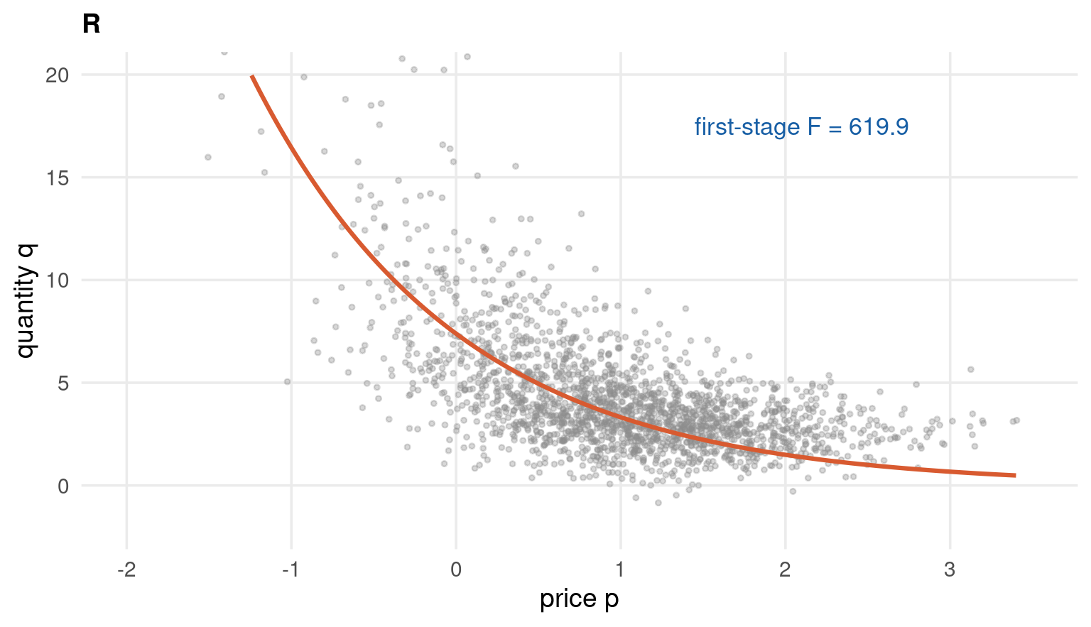
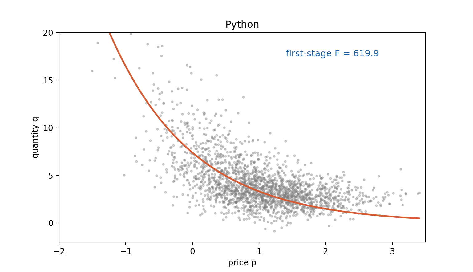
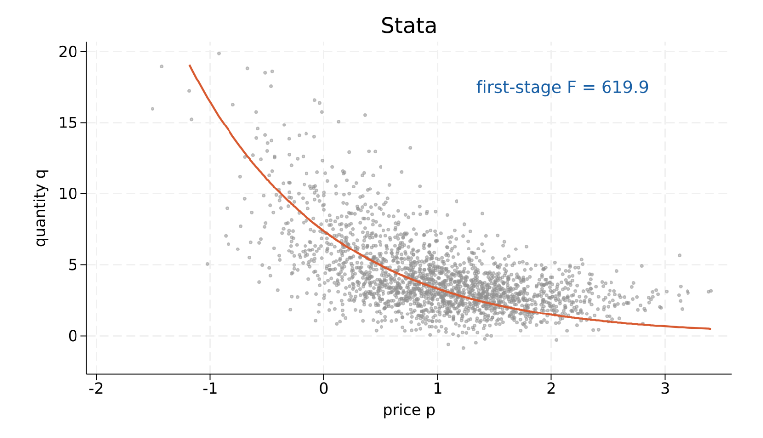
The curve is the conditional mean the model claims, drawn at \(x_i = 0\). The cloud around it is the endogeneity we are about to fight: high-price observations are not a random sample.

curve_df <- data.frame(p = seq(-1.5, 3.4, length.out = 400))
curve_df <- mutate(curve_df, q = exp(2.0 - 0.8 * p))
curve_df <- filter(curve_df, q <= 20)

ggplot(d) +
  aes(p, q) +
  geom_point(colour = "grey55", alpha = 0.35, size = 0.9) +
  geom_line(data = curve_df, colour = "#D85A30", linewidth = 1.1) +
  annotate("text", x = 2.1, y = 17.5, colour = "#185FA5", size = 4.5,
           label = "first-stage F = 619.9") +
  coord_cartesian(xlim = c(-2, 3.5), ylim = c(-2, 20)) +
  scale_x_continuous(breaks = -2:3) +
  scale_y_continuous(breaks = seq(0, 20, 5)) +
  labs(x = "price p", y = "quantity q", title = "R")

import matplotlib.pyplot as plt

pp = np.linspace(-1.5, 3.4, 400)
mm = np.exp(2.0 - 0.8 * pp)
keep = mm <= 20

fig, ax = plt.subplots(figsize = (8, 4.6))
sc = ax.scatter(d.p, d.q, s = 5, color = "grey", alpha = 0.35)
ln = ax.plot(pp[keep], mm[keep], color = "#D85A30", lw = 2)
txt = ax.text(2.1, 17.5, f"first-stage F = {first.fvalue:.1f}",
              color = "#185FA5", fontsize = 11, ha = "center")   # ggplot centres too
axopts = ax.set(xlim = (-2, 3.5), ylim = (-2, 20),
                xticks = range(-2, 4), yticks = range(0, 21, 5),
                xlabel = "price p", ylabel = "quantity q", title = "Python")
plt.show()

quietly import delimited "../data/moments-dgp.csv", clear
quietly destring _all, replace
quietly generate double truemean = exp(2.0 - 0.8*p)
sort p

twoway (scatter q p if q <= 20, msize(vsmall) mcolor(gs9%40))                   ///
       (line truemean p if truemean <= 20,                                     ///
             lcolor("216 90 48") lwidth(medthick)),                            ///
       text(17.5 2.1 "first-stage F = 619.9", color("24 95 165") size(medium)) ///
       xscale(range(-2 3.5)) yscale(range(-2 20))                              ///
       xlabel(-2(1)3) ylabel(0(5)20)                                           ///
       xtitle("price p") ytitle("quantity q") legend(off)                      ///
       title("Stata") graphregion(color(white))

quietly graph export "../plots/moments-dgp-scatter.png", replace width(1600)

Estimation I — Method of Moments by Hand

There is no magic in a GMM package. Write the sample moments, pick a weight matrix, hand the quadratic form to an optimiser:

\[\hat\beta = \arg\min_\beta \ \bar g(\beta)' W \bar g(\beta)\]

\[\bar g(\beta) = \frac{1}{n}\sum_{i=1}^{n} z_i\big(q_i - e^{\beta_0+\beta_1 p_i+\beta_2 x_i}\big)\]

Z <- cbind(1, d$z1, d$z2, d$z3, d$z4, d$x)

gi <- function(b) {                       # n x 6 matrix of moment contributions
  r <- d$q - exp(b[1] + b[2]*d$p + b[3]*d$x)
  Z * r
}
obj <- function(b, W) {
  g <- colMeans(gi(b))
  as.numeric(t(g) %*% W %*% g)
}

step1 <- optim(c(0, 0, 0), obj, W = diag(6), method = "BFGS")
S     <- crossprod(gi(step1$par)) / nrow(d)      # optimal weight is S^-1
step2 <- optim(step1$par, obj, W = solve(S), method = "BFGS")

J <- nrow(d) * step2$value
cat(sprintf("one-step (W = I) : %.4f %.4f %.4f\n",
            step1$par[1], step1$par[2], step1$par[3]))
cat(sprintf("two-step         : %.4f %.4f %.4f\n",
            step2$par[1], step2$par[2], step2$par[3]))
cat(sprintf("truth            : %.4f %.4f %.4f\n", 2.0, -0.8, 0.4))
cat(sprintf("J = %.4f on 3 df, p = %.4f\n", J, pchisq(J, 3, lower.tail = FALSE)))

one-step (W = I) : 1.9945 -0.7806 0.3955

two-step         : 1.9947 -0.7817 0.3956

truth            : 2.0000 -0.8000 0.4000

J = 2.7943 on 3 df, p = 0.4244

from scipy.optimize import minimize
from scipy.stats import chi2

Z = np.column_stack([np.ones(len(d)), d.z1, d.z2, d.z3, d.z4, d.x])
n = len(d)

def gi(b):                                # n x 6 matrix of moment contributions
    r = d.q.values - np.exp(b[0] + b[1]*d.p.values + b[2]*d.x.values)
    return Z * r[:, None]

def obj(b, W):
    g = gi(b).mean(axis = 0)
    return g @ W @ g

step1 = minimize(obj, [0, 0, 0], args = (np.eye(6),), method = "BFGS")
S     = gi(step1.x).T @ gi(step1.x) / n           # optimal weight is S^-1
step2 = minimize(obj, step1.x, args = (np.linalg.inv(S),), method = "BFGS")

J = n * step2.fun
out = (f"one-step (W = I) : {step1.x[0]:.4f} {step1.x[1]:.4f} {step1.x[2]:.4f}\n"
       f"two-step         : {step2.x[0]:.4f} {step2.x[1]:.4f} {step2.x[2]:.4f}\n"
       f"truth            : {2.0:.4f} {-0.8:.4f} {0.4:.4f}\n"
       f"J = {J:.4f} on 3 df, p = {chi2.sf(J, 3):.4f}")
import sys; nch = sys.stdout.write(out + "\n"); sys.stdout.flush()

one-step (W = I) : 1.9945 -0.7806 0.3955
two-step         : 1.9947 -0.7817 0.3956
truth            : 2.0000 -0.8000 0.4000
J = 2.7943 on 3 df, p = 0.4244

quietly import delimited "../data/moments-dgp.csv", clear
quietly destring _all, replace

mata:
void gmmcrit(todo, b, q, p, x, Z, W, val, grad, hess) {
    r    = q :- exp(b[1] :+ b[2]*p :+ b[3]*x)
    gbar = mean(Z :* r)'
    val  = gbar' * W * gbar
}
q = st_data(., "q"); p = st_data(., "p"); x = st_data(., "x")
Z = (J(rows(q),1,1), st_data(., ("z1","z2","z3","z4","x")))
n = rows(q)

M = optimize_init()
optimize_init_evaluator(M, &gmmcrit());  optimize_init_evaluatortype(M, "d0")
optimize_init_which(M, "min");           optimize_init_technique(M, "nm")
optimize_init_tracelevel(M, "none")
optimize_init_nmsimplexdeltas(M, J(1,3,0.1))
optimize_init_params(M, (0,0,0))
optimize_init_argument(M, 1, q); optimize_init_argument(M, 2, p)
optimize_init_argument(M, 3, x); optimize_init_argument(M, 4, Z)
optimize_init_argument(M, 5, I(6))
b1 = optimize(M)

r = q :- exp(b1[1] :+ b1[2]*p :+ b1[3]*x)
S = quadcross(Z:*r, Z:*r)/n
optimize_init_argument(M, 5, invsym(S));  optimize_init_params(M, b1)
b2 = optimize(M)

r2  = q :- exp(b2[1] :+ b2[2]*p :+ b2[3]*x)
gb  = mean(Z :* r2)'
Jst = n * (gb' * invsym(S) * gb)
printf("one-step (W = I) : %9.4f %9.4f %9.4f\n", b1[1], b1[2], b1[3])
printf("two-step         : %9.4f %9.4f %9.4f\n", b2[1], b2[2], b2[3])
printf("truth            : %9.4f %9.4f %9.4f\n", 2.0, -0.8, 0.4)
printf("J = %6.4f on 3 df, p = %6.4f\n", Jst, chi2tail(3, Jst))
end

------------------------------------------------- mata (type end to exit) ----------------------------------------------
: void gmmcrit(todo, b, q, p, x, Z, W, val, grad, hess) {
>     r    = q :- exp(b[1] :+ b[2]*p :+ b[3]*x)
>     gbar = mean(Z :* r)'
>     val  = gbar' * W * gbar
> }
note: argument todo unused.
note: argument grad unused.
note: argument hess unused.

: q = st_data(., "q"); p = st_data(., "p"); x = st_data(., "x")

: Z = (J(rows(q),1,1), st_data(., ("z1","z2","z3","z4","x")))

: n = rows(q)

: 
: M = optimize_init()

: optimize_init_evaluator(M, &gmmcrit());  optimize_init_evaluatortype(M, "d0")

: optimize_init_which(M, "min");           optimize_init_technique(M, "nm")

: optimize_init_tracelevel(M, "none")

: optimize_init_nmsimplexdeltas(M, J(1,3,0.1))

: optimize_init_params(M, (0,0,0))

: optimize_init_argument(M, 1, q); optimize_init_argument(M, 2, p)

: optimize_init_argument(M, 3, x); optimize_init_argument(M, 4, Z)

: optimize_init_argument(M, 5, I(6))

: b1 = optimize(M)

: 
: r = q :- exp(b1[1] :+ b1[2]*p :+ b1[3]*x)

: S = quadcross(Z:*r, Z:*r)/n

: optimize_init_argument(M, 5, invsym(S));  optimize_init_params(M, b1)

: b2 = optimize(M)

: 
: r2  = q :- exp(b2[1] :+ b2[2]*p :+ b2[3]*x)

: gb  = mean(Z :* r2)'

: Jst = n * (gb' * invsym(S) * gb)

: printf("one-step (W = I) : %9.4f %9.4f %9.4f\n", b1[1], b1[2], b1[3])
one-step (W = I) :    1.9945   -0.7806    0.3955

: printf("two-step         : %9.4f %9.4f %9.4f\n", b2[1], b2[2], b2[3])
two-step         :    1.9947   -0.7818    0.3956

: printf("truth            : %9.4f %9.4f %9.4f\n", 2.0, -0.8, 0.4)
truth            :    2.0000   -0.8000    0.4000

: printf("J = %6.4f on 3 df, p = %6.4f\n", Jst, chi2tail(3, Jst))
J = 2.7947 on 3 df, p = 0.4244

: end
------------------------------------------------------------------------------------------------------------------------

Estimation II — Off the Shelf, and the Standard Errors

Same estimator, one line. The variance needs the Jacobian \(G = \mathbb{E}[\partial g_i / \partial \beta']\):

\[\widehat{\mathrm{Var}}(\hat\beta) = \frac{1}{n}\big(\hat G' \hat S^{-1} \hat G\big)^{-1}\]

Here \(G\) has a closed form, but a numerical Jacobian agrees with it to eleven decimals — so do not hand-derive one under deadline.

g <- function(b, dat) {
  r <- dat[, "q"] - exp(b[1] + b[2]*dat[, "p"] + b[3]*dat[, "x"])
  cbind(r, r*dat[, "z1"], r*dat[, "z2"], r*dat[, "z3"], r*dat[, "z4"], r*dat[, "x"])
}
fit <- gmm(g, x = as.matrix(d), t0 = c(0, 0, 0), type = "twoStep", vcov = "iid")
summary(fit)

# analytic Jacobian versus numDeriv, at the estimate
b  <- coef(fit)
mu <- exp(b[1] + b[2]*d$p + b[3]*d$x)
G_analytic <- -crossprod(Z, cbind(1, d$p, d$x) * mu) / nrow(d)
G_numeric  <- numDeriv::jacobian(function(bb) colMeans(gi(bb)), b)
cat(sprintf("max |analytic - numeric| = %.2e\n", max(abs(G_analytic - G_numeric))))

Two-step GMM (gmm package)

         Estimate Std. Error  t value Pr(>|t|)
Theta[1]   1.9947     0.0077 259.3758        0
Theta[2]  -0.7817     0.0126 -62.0860        0
Theta[3]   0.3956     0.0063  62.6377        0

J = 2.7992 on 3 df, p = 0.4236

max |analytic Jacobian - numeric Jacobian| = 2.19e-11

from statsmodels.sandbox.regression.gmm import GMM
import numdifftools as nd

class ExpGMM(GMM):
    def momcond(self, params):
        b0, b1, b2 = params
        r = self.endog - np.exp(b0 + b1*self.exog[:, 0] + b2*self.exog[:, 1])
        return self.instrument * r[:, None]

mod = ExpGMM(endog = d.q.values, exog = d[["p", "x"]].values,
             instrument = Z, k_moms = 6, k_params = 3)
res = mod.fit(np.array([0.0, 0.0, 0.0]), maxiter = 2, optim_method = "bfgs",
              optim_args = {"disp": 0}, wargs = dict(centered = False))

b  = res.params
mu = np.exp(b[0] + b[1]*d.p.values + b[2]*d.x.values)
G_analytic = -Z.T @ (np.column_stack([np.ones(n), d.p, d.x]) * mu[:, None]) / n
G_numeric  = nd.Jacobian(lambda bb: gi(bb).mean(axis = 0))(b)

jstat, jpval, jdf = res.jtest()
lines = [f"b{k}   {b[k]:9.4f}   {res.bse[k]:9.4f}" for k in range(3)]
out = ("Two-step GMM (statsmodels)\n"
       "        estimate   std.error\n" + "\n".join(lines)
       + f"\n\nJ = {jstat:.4f} on {jdf} df, p = {jpval:.4f}\n"
       + "max |analytic Jacobian - numeric Jacobian| = "
       + f"{np.abs(G_analytic - G_numeric).max():.2e}")
import sys; nch = sys.stdout.write(out + "\n"); sys.stdout.flush()

Two-step GMM (statsmodels)
        estimate   std.error
b0      1.9947      0.0077
b1     -0.7817      0.0126
b2      0.3956      0.0063

J = 2.7943 on 3 df, p = 0.4244
max |analytic Jacobian - numeric Jacobian| = 5.21e-14

quietly import delimited "../data/moments-dgp.csv", clear
quietly destring _all, replace

gmm (q - exp({b0} + {b1}*p + {b2}*x)), instruments(z1 z2 z3 z4 x) twostep nolog
estat overid

Final GMM criterion Q(b) = .0013945

GMM estimation 

Number of parameters =   3
Number of moments    =   6
Initial weight matrix: Unadjusted                 Number of obs   =      2,000
GMM weight matrix:     Robust

------------------------------------------------------------------------------
             |               Robust
             | Coefficient  std. err.      z    P>|z|     [95% conf. interval]
-------------+----------------------------------------------------------------
         /b0 |   1.994709   .0076905   259.37   0.000     1.979636    2.009782
         /b1 |  -.7817255   .0125911   -62.09   0.000    -.8064035   -.7570474
         /b2 |   .3955544   .0063152    62.64   0.000     .3831768     .407932
------------------------------------------------------------------------------
Instruments for equation 1: z1 z2 z3 z4 x _cons


  Test of overidentifying restriction:

  Hansen's J chi2(3) = 2.78906 (p = 0.4253)

Stata differentiates the residual expression symbolically, so there is no Jacobian to supply and nothing to check by hand.

Results Table

• Results
• LaTeX

All numbers from the R column; Python and Stata agree to four decimals.

	\(\beta_0\)	\(\beta_1\) (semi-elasticity)	\(\beta_2\)
Truth	2.0000	−0.8000	0.4000
NLS (ignores endogeneity)	1.9016	−0.6831	0.4205
GMM one-step, \(W = I\)	1.9944	−0.7805	0.3955
GMM two-step	1.9947	−0.7817	0.3956
GMM iterated	1.9947	−0.7817	0.3956
GMM continuously updated	1.9950	−0.7824	0.3956
two-step std. error	0.0077	0.0126	0.0063

NLS puts the semi-elasticity at −0.68 when the truth is −0.80: a 15% attenuation, and it is not noise — the two-step standard error is 0.0126, so the gap is nearly eight standard errors wide.

\[\hat\beta_1^{\,\text{NLS}} = -0.6831 \quad\text{vs}\quad \hat\beta_1^{\,\text{GMM}} = -0.7817 \ (0.0126)\]

Every GMM variant lands within one standard error of the truth. The \(J\) statistic is 2.80 on 3 degrees of freedom (\(p = 0.42\)): the three over-identifying restrictions are not rejected, which is what a correctly specified model looks like.

\begin{tabular}{lccc}
\hline
                    & $\beta_0$ & $\beta_1$ & $\beta_2$ \\
\hline
Truth               &  2.0000 & $-0.8000$ & 0.4000 \\
NLS                 &  1.9016 & $-0.6831$ & 0.4205 \\
GMM one-step        &  1.9944 & $-0.7805$ & 0.3955 \\
GMM two-step        &  1.9947 & $-0.7817$ & 0.3956 \\
                    & (0.0077)& (0.0126)  & (0.0063)\\
GMM iterated        &  1.9947 & $-0.7817$ & 0.3956 \\
GMM CUE             &  1.9950 & $-0.7824$ & 0.3956 \\
\hline
\multicolumn{4}{l}{\footnotesize $J = 2.799$ (3 df), $p = 0.424$, $n = 2000$.}
\end{tabular}

library(modelsummary)
modelsummary(list("Two-step" = two, "Iterated" = ite, "CUE" = cue),
             estimate  = "{estimate}",
             statistic = "({std.error})",
             gof_map   = c("nobs"),
             output    = "latex")

tab = pd.DataFrame({"estimate": res.params, "std.error": res.bse},
                   index = ["b0", "b1", "b2"])
print(tab.round(4).to_latex())

quietly gmm (q - exp({b0} + {b1}*p + {b2}*x)), ///
    instruments(z1 z2 z3 z4 x) twostep
estimates store twostep
esttab twostep using "results.tex", se b(%9.4f) replace

Estimating \(S\) — the Weight That Makes GMM Efficient

• The Object

The efficient weight is the inverse of the long-run variance of the moments:

\[S = \lim_{n\to\infty} \mathrm{Var}\Big(\sqrt{n}\,\bar g(\beta_0)\Big) = \sum_{j=-\infty}^{\infty} \mathbb{E}\big[g_i(\beta_0)\,g_{i-j}(\beta_0)'\big]\]

Which estimator of \(S\) you use is a modelling decision, not a default:

• iid — only if the errors are homoskedastic
• heteroskedasticity-robust — \(\hat S = n^{-1}\sum_i g_i g_i'\), the cross-section default
• cluster — sum within clusters first; use when sampling is grouped
• HAC — for time series, where the \(j \neq 0\) terms do not vanish:

\[\hat S_{\text{HAC}} = \hat\Gamma_0 + \sum_{j=1}^{n-1} k\!\left(\frac{j}{b_n}\right)\big(\hat\Gamma_j + \hat\Gamma_j'\big)\]

On this DGP the errors are homoskedastic by construction, so iid and robust agree to four decimals — 0.0077 / 0.0126 / 0.0063 either way. That is the exception, not the rule. Part 5 estimates an Euler equation where the kernel and bandwidth move the standard errors substantially.

kern <- data.frame(u = seq(0, 3, by = 0.005))
kern <- mutate(kern,
  Bartlett = pmax(0, 1 - u),
  Parzen   = ifelse(u <= 0.5, 1 - 6*u^2 + 6*u^3,
              ifelse(u <= 1, 2*(1 - u)^3, 0)),
  arg      = 6*pi*u/5,
  QS       = ifelse(u == 0, 1,
              25/(12*pi^2*u^2) * (sin(arg)/arg - cos(arg))))

long <- pivot_longer(kern, c(Bartlett, Parzen, QS),
                     names_to = "kernel", values_to = "w")

ggplot(long) +
  aes(u, w, colour = kernel) +
  geom_hline(yintercept = 0, colour = "grey70", linetype = "dashed") +
  geom_line(linewidth = 1.1) +
  scale_colour_manual(values = c("Bartlett" = "#185FA5",
                                 "Parzen"   = "#1D9E75",
                                 "QS"       = "#D85A30")) +
  coord_cartesian(xlim = c(0, 3), ylim = c(-0.2, 1)) +
  scale_x_continuous(breaks = 0:3) +
  scale_y_continuous(breaks = seq(-0.2, 1, 0.2)) +
  labs(x = "lag / bandwidth", y = "kernel weight", colour = NULL, title = "R")

u = np.arange(0, 3.0005, 0.005)
bartlett = np.maximum(0, 1 - u)
parzen = np.where(u <= 0.5, 1 - 6*u**2 + 6*u**3,
                  np.where(u <= 1, 2*(1 - u)**3, 0))
arg = 6*np.pi*u/5
with np.errstate(divide = "ignore", invalid = "ignore"):
    qs = 25/(12*np.pi**2*u**2) * (np.sin(arg)/arg - np.cos(arg))
qs[0] = 1.0

fig, ax = plt.subplots(figsize = (8, 4.6))
ln = ax.axhline(0, color = "grey", ls = "--", lw = 1)
ln = ax.plot(u, bartlett, color = "#185FA5", lw = 2, label = "Bartlett")
ln = ax.plot(u, parzen,   color = "#1D9E75", lw = 2, label = "Parzen")
ln = ax.plot(u, qs,       color = "#D85A30", lw = 2, label = "QS")
leg = ax.legend(loc = "upper right", frameon = False)
axopts = ax.set(xlim = (0, 3), ylim = (-0.2, 1),
                xticks = range(0, 4), yticks = np.arange(-0.2, 1.01, 0.2),
                xlabel = "lag / bandwidth", ylabel = "kernel weight",
                title = "Python")
plt.show()

clear
quietly set obs 601
quietly generate double u = (_n - 1)/200
quietly generate double bartlett = max(0, 1 - u)
quietly generate double parzen = cond(u <= 0.5, 1 - 6*u^2 + 6*u^3, ///
                                      cond(u <= 1, 2*(1 - u)^3, 0))
quietly generate double arg = 6*_pi*u/5
quietly generate double qs = cond(u == 0, 1, ///
    25/(12*_pi^2*u^2) * (sin(arg)/arg - cos(arg)))

twoway (line bartlett u, lcolor("24 95 165") lwidth(medthick))                 ///
       (line parzen u,   lcolor("29 158 117") lwidth(medthick))                ///
       (line qs u,       lcolor("216 90 48") lwidth(medthick)),                ///
       yline(0, lcolor(gs10) lpattern(dash))                                   ///
       xscale(range(0 3)) yscale(range(-0.2 1))                                ///
       xlabel(0(1)3) ylabel(-0.2(0.2)1.0)                                      ///
       xtitle("lag / bandwidth") ytitle("kernel weight")                       ///
       legend(order(1 "Bartlett" 2 "Parzen" 3 "QS") rows(1))                   ///
       title("Stata") graphregion(color(white))

quietly graph export "../plots/moments-kernels.png", replace width(1600)

The Estimator Zoo — One Step, Two, Many, or Continuous

Four ways to handle the fact that the efficient weight depends on the parameter you are trying to estimate:

• one-step — fix \(W = I\); consistent, not efficient
• two-step — estimate \(\hat S\) at the one-step \(\hat\beta\), minimise once more
• iterated — repeat until \(\hat\beta\) stops moving
• continuously updated — let \(W\) depend on \(\beta\) inside the optimiser:

\[\hat\beta_{\text{CUE}} = \arg\min_\beta \ \bar g(\beta)' \hat S(\beta)^{-1} \bar g(\beta)\]

one <- gmm(g, as.matrix(d), t0 = c(0,0,0), type = "twoStep",
           vcov = "iid", wmatrix = "ident")
two <- gmm(g, as.matrix(d), t0 = c(0,0,0), type = "twoStep",   vcov = "iid")
ite <- gmm(g, as.matrix(d), t0 = c(0,0,0), type = "iterative", vcov = "iid")
# CUE needs a warm start: from c(0,0,0) the weight matrix is singular
cue <- gmm(g, as.matrix(d), t0 = coef(two), type = "cue", vcov = "iid")

data.frame(estimator = c("one-step (W=I)", "two-step", "iterated", "CUE", "truth"),
           b0 = c(coef(one)[1], coef(two)[1], coef(ite)[1], coef(cue)[1],  2.0),
           b1 = c(coef(one)[2], coef(two)[2], coef(ite)[2], coef(cue)[2], -0.8),
           b2 = c(coef(one)[3], coef(two)[3], coef(ite)[3], coef(cue)[3],  0.4))

      estimator     b0      b1     b2
 one-step (W=I) 1.9944 -0.7805 0.3955
       two-step 1.9947 -0.7817 0.3956
       iterated 1.9947 -0.7817 0.3956
            CUE 1.9950 -0.7824 0.3956
          truth 2.0000 -0.8000 0.4000

def gmm_fit(iters):
    b = minimize(obj, [0, 0, 0], args = (np.eye(6),), method = "BFGS").x
    for _ in range(iters):
        Sk = gi(b).T @ gi(b) / n
        b  = minimize(obj, b, args = (np.linalg.inv(Sk),), method = "BFGS").x
    return b

def cue_obj(b):
    G = gi(b)
    gb = G.mean(axis = 0)
    return gb @ np.linalg.inv(G.T @ G / n) @ gb

one = gmm_fit(0)
two = gmm_fit(1)
ite = gmm_fit(40)
cue = minimize(cue_obj, two, method = "BFGS").x      # warm start, as in R

rows = [("one-step (W=I)", one), ("two-step", two), ("iterated", ite),
        ("CUE", cue), ("truth", np.array([2.0, -0.8, 0.4]))]
out = f"{'estimator':<16}{'b0':>10}{'b1':>10}{'b2':>10}\n" + "\n".join(
    f"{nm:<16}{v[0]:>10.4f}{v[1]:>10.4f}{v[2]:>10.4f}" for nm, v in rows)
import sys; nch = sys.stdout.write(out + "\n"); sys.stdout.flush()

estimator               b0        b1        b2
one-step (W=I)      1.9945   -0.7806    0.3955
two-step            1.9947   -0.7817    0.3956
iterated            1.9947   -0.7817    0.3956
CUE                 1.9950   -0.7824    0.3956
truth               2.0000   -0.8000    0.4000

quietly import delimited "../data/moments-dgp.csv", clear
quietly destring _all, replace

quietly gmm (q - exp({b0} + {b1}*p + {b2}*x)), ///
    instruments(z1 z2 z3 z4 x) onestep nolog
display "one-step : " %9.4f _b[b0:_cons] %9.4f _b[b1:_cons] %9.4f _b[b2:_cons]

quietly gmm (q - exp({b0} + {b1}*p + {b2}*x)), ///
    instruments(z1 z2 z3 z4 x) twostep nolog
display "two-step : " %9.4f _b[b0:_cons] %9.4f _b[b1:_cons] %9.4f _b[b2:_cons]

quietly gmm (q - exp({b0} + {b1}*p + {b2}*x)), ///
    instruments(z1 z2 z3 z4 x) igmm nolog
display "iterated : " %9.4f _b[b0:_cons] %9.4f _b[b1:_cons] %9.4f _b[b2:_cons]
display "truth    : " %9.4f 2.0 %9.4f -0.8 %9.4f 0.4

one-step :    1.9946  -0.7814   0.3955


two-step :    1.9947  -0.7817   0.3956


iterated :    1.9947  -0.7817   0.3956

truth    :    2.0000  -0.8000   0.4000

Stata’s gmm has no CUE option. The R and Python tabs show it; on this sample it lands 0.0007 from the two-step estimate.

The GMM Objective Surface

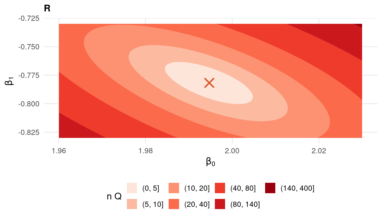
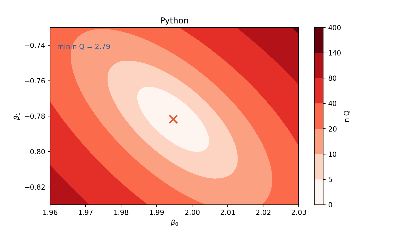
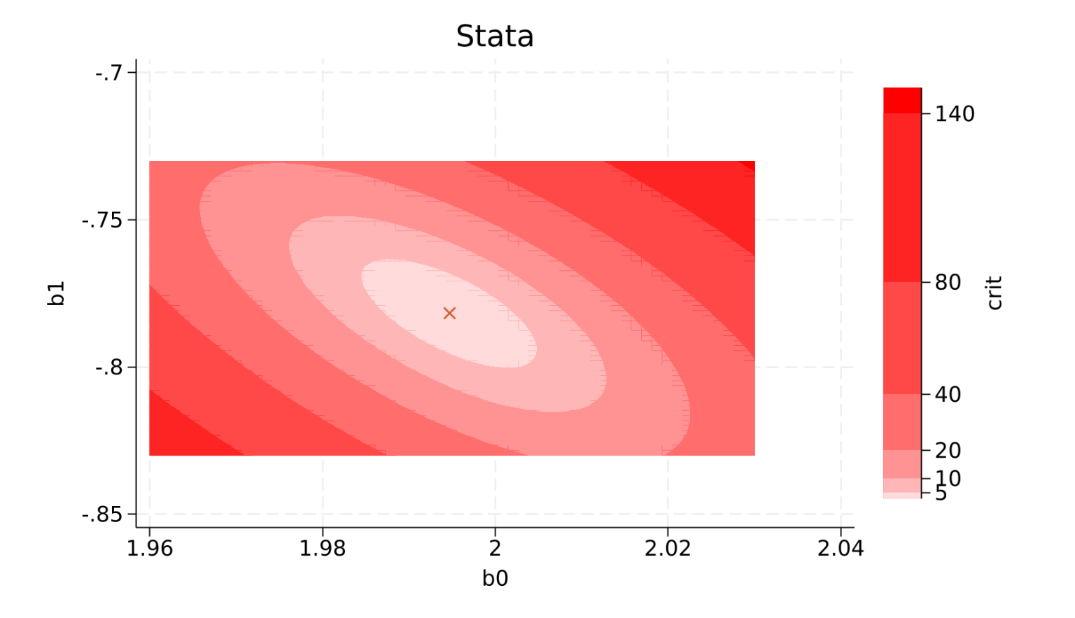
Contours of \(n\,\bar g(\beta)'\hat S^{-1}\bar g(\beta)\) over \((\beta_0,\beta_1)\), with \(\beta_2\) held at its estimate. The valley runs diagonally: intercept and slope trade off against each other, which is exactly why their estimates are correlated.

bhat <- coef(fit)
Shat <- crossprod(gi(bhat)) / nrow(d)
Winv <- solve(Shat)

crit <- function(b0, b1) {
  gb <- colMeans(gi(c(b0, b1, bhat[3])))
  nrow(d) * as.numeric(t(gb) %*% Winv %*% gb)
}
grid <- expand.grid(b0 = seq(1.96, 2.03, length.out = 60),
                    b1 = seq(-0.83, -0.73, length.out = 60))
grid <- mutate(grid, Q = mapply(crit, b0, b1))

ggplot(grid) +
  aes(b0, b1, z = Q) +
  geom_contour_filled(breaks = c(0, 5, 10, 20, 40, 80, 140, 400)) +
  annotate("point", x = bhat[1], y = bhat[2], shape = 4, size = 5,
           stroke = 1.6, colour = "#D85A30") +
  scale_fill_brewer(palette = "Reds", direction = 1) +
  labs(x = expression(beta[0]), y = expression(beta[1]),
       fill = "n Q", title = "R")

bhat = res.params
Winv = np.linalg.inv(gi(bhat).T @ gi(bhat) / n)

b0g = np.linspace(1.96, 2.03, 60)
b1g = np.linspace(-0.83, -0.73, 60)
Q = np.array([[n * (lambda gb: gb @ Winv @ gb)(gi([a, b, bhat[2]]).mean(axis = 0))
               for a in b0g] for b in b1g])

from matplotlib.colors import BoundaryNorm

levels = [0, 5, 10, 20, 40, 80, 140, 400]
# colour each band by its index, as ggplot and Stata do; a plain linear norm
# over 0-400 would wash the low bands out and break the cross-tab match
norm = BoundaryNorm(levels, ncolors = 256)

fig, ax = plt.subplots(figsize = (8, 4.6))
cs = ax.contourf(b0g, b1g, Q, levels = levels, cmap = "Reds", norm = norm)
ln = ax.plot(bhat[0], bhat[1], "x", ms = 11, mew = 2.2, color = "#D85A30")
txt = ax.text(1.962, -0.742, f"min n Q = {Q.min():.2f}", fontsize = 10,
              color = "#185FA5")
cb = fig.colorbar(cs, ax = ax, label = "n Q")
axopts = ax.set(xlabel = r"$\beta_0$", ylabel = r"$\beta_1$", title = "Python")
plt.show()

quietly import delimited "../data/moments-dgp.csv", clear
quietly destring _all, replace

mata:
q = st_data(., "q"); p = st_data(., "p"); x = st_data(., "x")
Z = (J(rows(q),1,1), st_data(., ("z1","z2","z3","z4","x")))
n = rows(q)
b = (1.994709, -0.7817255, 0.3955544)
r = q :- exp(b[1] :+ b[2]*p :+ b[3]*x)
W = invsym(quadcross(Z:*r, Z:*r)/n)
nb = 60
b0g = rangen(1.96, 2.03, nb); b1g = rangen(-0.83, -0.73, nb)
out = J(nb*nb, 3, .); k = 1
for (i=1; i<=nb; i++) {
  for (j=1; j<=nb; j++) {
    rr = q :- exp(b0g[i] :+ b1g[j]*p :+ b[3]*x)
    gb = mean(Z :* rr)'
    out[k,] = (b0g[i], b1g[j], n*(gb'*W*gb))
    k++
  }
}
end

preserve
clear
quietly set obs 3600
quietly generate double b0v = .
quietly generate double b1v = .
quietly generate double crit = .
mata: st_store(., ("b0v","b1v","crit"), out)

twoway (contour crit b1v b0v, ccuts(5 10 20 40 80 140) crule(intensity))      ///
       (scatteri -0.7817 1.9947, msymbol(X) msize(large)                      ///
                 mcolor("216 90 48")),                                        ///
       xtitle("b0") ytitle("b1") legend(off) title("Stata")                   ///
       graphregion(color(white))

quietly graph export "../plots/moments-objsurface.png", replace width(1600)
restore

Two Ways to Get a Wrong Answer

Both failures below happened while building this deck. Neither printed an error that named the real cause.

Starting values. CUE from \(\beta^{(0)} = (0,0,0)\) dies with system is computationally singular: far from the truth the residuals are enormous and nearly collinear, so \(\hat S(\beta)\) cannot be inverted. Started from the two-step estimate it converges immediately.

Scaling. The criterion is not invariant to how the moments are scaled. Multiply one instrument by 1000 and the one-step estimate changes, because \(W = I\) silently declares every moment equally important. The two-step estimator is invariant — \(\hat S^{-1}\) undoes the scaling — which is one more reason not to report one-step numbers as final.

Why two-step is scale-invariant

Rescale the moments by any non-singular \(A\), so that \(\tilde g(\beta) = A\,\bar g(\beta)\). The variance rescales the same way:

\[ \tilde S = A S A' \]

Put both into the two-step criterion and the \(A\) matrices cancel exactly:

\[ \tilde g' \tilde S^{-1} \tilde g = \bar g' A' (A S A')^{-1} A \bar g = \bar g' S^{-1} \bar g \]

So the two-step estimate, the \(J\) statistic and the standard errors are all unchanged. With \(W = I\) there is no \(\hat S\) to absorb \(A\), and the estimate moves. The practical rule: report one-step results only as a starting value or a robustness check, never as the headline. If you must use \(W = I\), scale the instruments to comparable magnitudes first.

A starting-value recipe that works

In order, stopping as soon as one succeeds:

• A consistent-but-inefficient estimator. Here NLS gets \(\beta_1\) wrong by 15%, but it is a perfectly good place to start from.
• One-step GMM with \(W = I\). Cheap, nothing to invert, and the objective is well behaved far from the optimum.
• A coarse grid search over an economically sensible box, then a local optimiser from the best grid point. Slow, but it will not miss a basin.
• A derivative-free optimiser (Nelder–Mead) for the first pass, then BFGS to polish. The Stata tabs in this deck use exactly that pattern in Mata.

What not to do: start every parameter at zero because it looks tidy. With \(\exp(\cdot)\) inside the model, \(\beta = 0\) makes every fitted value equal to 1, the residuals enormous, and \(\hat S(\beta)\) near-singular — which is precisely the CUE failure described on this slide.

Part 3 — Overidentification and Finite Samples

The \(J\) Test — What the Spare Equations Buy You

• The Statistic
• What Rejection Means
• Testing a Subset — the \(C\) Statistic

With \(q > k\) the moments cannot all be set to zero. If the model is right, what remains should be small — no larger than sampling error. Scale the minimised criterion by \(n\) and it has a known distribution:

\[J = n \, \bar g(\hat\theta)' \hat S^{-1} \bar g(\hat\theta) \ \xrightarrow{\ d\ } \ \chi^2_{q-k}\]

Reject when \(J\) exceeds the \(\chi^2_{q-k}\) critical value, i.e. when \(p < 0.05\) at the 5% level. On the Part 2 DGP: \(q - k = 3\), so the critical value is \(\chi^2_{3,0.95} = 7.81\).

\(J\) tests the moments jointly. A rejection says at least one of the over-identifying restrictions is false. It does not say which, and it does not say the parameter estimate is useless.

Equally important, the converse is weak:

• \(J\) has no power against anything that shifts all moments together. If every instrument is invalid in the same direction, \(\bar g\) can be small at a wrong \(\hat\theta\) and \(J\) passes serenely
• Non-rejection is not validation. With few observations or many moments, \(J\) is under-powered; Part 8 shows it losing power precisely when the estimator is most biased
• The estimated \(\hat S\) is inside the statistic. A badly estimated weight matrix distorts \(J\) before you ever look at the p-value

To ask which moments are suspect, compare the \(J\) from the full set with the \(J\) from a subset you are willing to defend:

\[C = J_{\text{full}} - J_{\text{subset}} \ \xrightarrow{\ d\ } \ \chi^2_{r}\]

where \(r\) is the number of moments dropped. Both must use the same \(\hat S\) block and the same sample, or the difference is not a \(\chi^2\). This is Eichenbaum, Hansen and Singleton’s difference test; Part 8 uses it as the engine of moment selection.

\(J\) and \(C\) — Code

Drop the two weakest instruments \((z_3, z_4)\) and ask whether the data object to putting them back.

g6 <- function(b, dat) {                      # all six moments
  r <- dat[, "q"] - exp(b[1] + b[2]*dat[, "p"] + b[3]*dat[, "x"])
  cbind(r, r*dat[, "z1"], r*dat[, "z2"], r*dat[, "z3"], r*dat[, "z4"], r*dat[, "x"])
}
g4 <- function(b, dat) {                      # z3 and z4 removed
  r <- dat[, "q"] - exp(b[1] + b[2]*dat[, "p"] + b[3]*dat[, "x"])
  cbind(r, r*dat[, "z1"], r*dat[, "z2"], r*dat[, "x"])
}
full <- gmm(g6, as.matrix(d), t0 = c(0,0,0), type = "twoStep", vcov = "iid")
sub  <- gmm(g4, as.matrix(d), t0 = c(0,0,0), type = "twoStep", vcov = "iid")

Jf <- summary(full)$stest$test
Js <- summary(sub)$stest$test
C  <- Jf[1] - Js[1]
cat(sprintf("J full    : %.4f on 3 df, p = %.4f\n", Jf[1], Jf[2]))
cat(sprintf("J subset  : %.4f on 1 df, p = %.4f\n", Js[1], Js[2]))
cat(sprintf("C = Jf-Js : %.4f on 2 df, p = %.4f\n", C, pchisq(C, 2, lower.tail = FALSE)))

J full    : 2.7992 on 3 df, p = 0.4236

J subset  : 0.0489 on 1 df, p = 0.8250

C = Jf-Js : 2.7503 on 2 df, p = 0.2528

critical values: chi2(3) = 7.81, chi2(2) = 5.99

verdict: neither test rejects. z3 and z4 are admissible.

import numpy as np, pandas as pd
from scipy.optimize import minimize
from scipy.stats import chi2

dg = pd.read_csv("../data/moments-dgp.csv")
n  = len(dg)

def fit_J(cols):                          # two-step GMM, returns (theta, J, df)
    Z = np.column_stack([np.ones(n)] + [dg[c].values for c in cols])
    gi = lambda b: Z * (dg.q.values - np.exp(b[0] + b[1]*dg.p.values
                                                  + b[2]*dg.x.values))[:, None]
    obj = lambda b, W: gi(b).mean(axis=0) @ W @ gi(b).mean(axis=0)
    b1 = minimize(obj, [0,0,0], args=(np.eye(Z.shape[1]),), method="BFGS").x
    S  = gi(b1).T @ gi(b1) / n
    b2 = minimize(obj, b1, args=(np.linalg.inv(S),), method="BFGS").x
    return b2, n*obj(b2, np.linalg.inv(S)), Z.shape[1] - 3

_, Jf, dff = fit_J(["z1", "z2", "z3", "z4", "x"])      # all six moments
_, Js, dfs = fit_J(["z1", "z2", "x"])                  # z3 and z4 removed
C = Jf - Js

out = (f"J full    : {Jf:.4f} on {dff} df, p = {chi2.sf(Jf, dff):.4f}\n"
       f"J subset  : {Js:.4f} on {dfs} df, p = {chi2.sf(Js, dfs):.4f}\n"
       f"C = Jf-Js : {C:.4f} on 2 df, p = {chi2.sf(C, 2):.4f}\n\n"
       f"critical values: chi2(3) = {chi2.ppf(0.95,3):.2f}, "
       f"chi2(2) = {chi2.ppf(0.95,2):.2f}\n"
       f"verdict: neither test rejects. z3 and z4 are admissible.")
import sys; nch = sys.stdout.write(out + "\n"); sys.stdout.flush()

J full    : 2.7943 on 3 df, p = 0.4244
J subset  : 0.0488 on 1 df, p = 0.8252
C = Jf-Js : 2.7455 on 2 df, p = 0.2534

critical values: chi2(3) = 7.81, chi2(2) = 5.99
verdict: neither test rejects. z3 and z4 are admissible.

quietly import delimited "../data/moments-dgp.csv", clear
quietly destring _all, replace

quietly gmm (q - exp({b0} + {b1}*p + {b2}*x)), ///
    instruments(z1 z2 z3 z4 x) twostep nolog
estat overid
scalar Jfull = r(J)

quietly gmm (q - exp({b0} + {b1}*p + {b2}*x)), ///
    instruments(z1 z2 x) twostep nolog
estat overid
scalar Jsub = r(J)

scalar C = Jfull - Jsub
display "C = Jfull - Jsub = " %6.4f C " on 2 df, p = " %6.4f chi2tail(2, C)
display "verdict: neither test rejects. z3 and z4 are admissible."

  Test of overidentifying restriction:

  Hansen's J chi2(3) = 2.78906 (p = 0.4253)




  Test of overidentifying restriction:

  Hansen's J chi2(1) = .048802 (p = 0.8252)



C = Jfull - Jsub = 2.7403 on 2 df, p = 0.2541

verdict: neither test rejects. z3 and z4 are admissible.

Why Two-Step GMM Is Biased in Finite Samples

The efficient weight \(\hat S^{-1}\) is not a constant — it is estimated from the same data used to form \(\bar g\). That correlation is the whole problem.

\[\hat S = \frac{1}{n}\sum_{i=1}^n g_i(\tilde\theta)\, g_i(\tilde\theta)' \qquad\text{is correlated with}\qquad \bar g(\theta)\]

An observation with a large moment contribution inflates its own entry in \(\hat S\), so the second step down-weights precisely the observations that were pushing the estimate. The estimator is pulled towards parameter values that make the estimated weight look favourable — a bias of order \(1/n\) that grows with the number of moments \(q\).

Two consequences, both visible in the Monte Carlo two slides on:

• adding moments raises asymptotic efficiency but worsens finite-sample bias — the trade-off Part 8 formalises
• estimators that never form a separate \(\hat S\) from a preliminary \(\tilde\theta\) — CUE, empirical likelihood — do not inherit this term

\[\mathbb{E}\big[\hat\theta_{\text{2-step}}\big] - \theta_0 = \frac{\text{something} \times q}{n} + O(n^{-2})\]

CUE and the GEL Family

• CUE
• The GEL Family
• The Dual

Stop treating the weight as a constant. Let it depend on \(\theta\) inside the minimisation:

\[\hat\theta_{\text{CUE}} = \arg\min_\theta \ \bar g(\theta)' \hat S(\theta)^{-1} \bar g(\theta)\]

There is no preliminary estimate and no separate weighting step, so the bias term above never appears. The price is a criterion that is no longer a simple quadratic: it can be flat or multi-modal in the tails, which is why CUE failed from a cold start in Part 2 and why its RMSE is the largest in the Monte Carlo.

Generalised empirical likelihood attacks the problem from the other side. Instead of weighting moments, reweight observations: choose probabilities \(p_i\) as close as possible to \(1/n\) subject to the moments holding exactly under \(p\).

\[\max_{\theta,\, p} \ \sum_{i=1}^{n} h(p_i) \quad \text{s.t.} \quad \sum_{i=1}^n p_i\, g_i(\theta) = 0, \quad \sum_{i=1}^n p_i = 1\]

The choice of \(h\) names the member:

\(h(p_i)\)	Name	Also known as
\(\log p_i\)	Empirical likelihood (EL)	Owen (1988), Qin & Lawless
\(-p_i \log p_i\)	Exponential tilting (ET)	Kitamura & Stutzer
\(-(p_i)^2\)	CUE	the GEL member with a quadratic \(h\)

All three are \(\sqrt{n}\)-consistent, asymptotically equivalent to efficient GMM, and share its asymptotic variance. They differ in the higher-order term — and Newey & Smith (2004) show EL removes the bias component that grows with \(q\).

The constrained problem above has \(n\) unknowns. Its dual has only \(q\): a multiplier \(\lambda\) on the moment constraint, solved by an inner concave maximisation, with the implied probabilities recovered afterwards.

\[\hat\lambda(\theta) = \arg\max_{\lambda} \ \sum_{i=1}^{n} \log\!\big(1 + \lambda' g_i(\theta)\big), \qquad \hat p_i = \frac{1}{n\big(1 + \hat\lambda' g_i\big)}\]

\[-2 \log \mathrm{ELR}(\theta) = 2 \sum_{i=1}^{n} \log\!\big(1 + \hat\lambda' g_i(\theta)\big) \ \xrightarrow{\ d\ } \ \chi^2_{q-k}\]

The profile criterion is an over-identification statistic in its own right — the EL counterpart of \(J\), and it lands on 2.80 here, essentially on top of it.

The convex-hull condition. The dual is only defined when \(0\) lies inside the convex hull of \(\{g_i(\theta)\}\). Outside it, no set of positive \(p_i\) can satisfy the constraint and EL is \(+\infty\). Any hand-written implementation must return a penalty there — omit that guard and the optimiser escapes to a region where the criterion is finite but meaningless.

Empirical Likelihood — Code

The R tab uses gmm::gel. The Python and Stata tabs hand-code the dual, because neither language ships an EL routine — inner Newton iteration with step-halving, and the convex-hull guard from the previous slide.

two <- gmm(g6, as.matrix(d), t0 = c(0,0,0), type = "twoStep", vcov = "iid")
el  <- gel(g6, as.matrix(d), tet0 = coef(two), type = "EL")
et  <- gel(g6, as.matrix(d), tet0 = coef(two), type = "ET")
cu  <- gel(g6, as.matrix(d), tet0 = coef(two), type = "CUE")

for (f in list(el, et, cu)) print(round(coef(f), 4))
summary(el)$stest$test        # the EL over-identification statistic

    estimator     b0      b1     b2 overid
 two-step GMM 1.9947 -0.7817 0.3956  2.799
           EL 1.9950 -0.7823 0.3956  2.796
           ET 1.9950 -0.7823 0.3956  2.795
          CUE 1.9950 -0.7824 0.3956  2.783
        truth 2.0000 -0.8000 0.4000     NA

All four agree to three decimals: with n = 2000 the members of the

family are indistinguishable. The Monte Carlo next uses n = 200.

Zg = np.column_stack([np.ones(n), dg.z1, dg.z2, dg.z3, dg.z4, dg.x])
gi = lambda b: Zg * (dg.q.values - np.exp(b[0] + b[1]*dg.p.values
                                               + b[2]*dg.x.values))[:, None]

def el_crit(b):
    """-2 log ELR at b: inner concave maximisation over lambda."""
    G = gi(b); m = G.shape[1]; lam = np.zeros(m)
    for _ in range(50):
        z = 1 + G @ lam
        if z.min() <= 1e-8:                      # outside the convex hull
            z = np.maximum(z, 1e-8)
        gr = (G / z[:, None]).sum(axis=0)
        H  = -(G / z[:, None]**2).T @ G
        try:
            step = np.linalg.solve(H - 1e-10*np.eye(m), gr)
        except np.linalg.LinAlgError:
            break
        f0 = np.sum(np.log(np.maximum(1 + G @ lam, 1e-12)))
        for h in range(13):                      # step-halving
            cand = lam - step/2**h
            zc = 1 + G @ cand
            if zc.min() > 1e-8:
                f1 = np.sum(np.log(zc))
                if f1 >= f0:
                    lam = cand
                    break
        if np.max(np.abs(step)) < 1e-10:
            break
    z = 1 + G @ lam
    if z.min() <= 1e-8:
        return 1e6                               # convex-hull guard
    return 2*np.sum(np.log(z))

b_two = fit_J(["z1", "z2", "z3", "z4", "x"])[0]
r_el  = minimize(el_crit, b_two, method="Nelder-Mead",
                 options=dict(maxiter=800, fatol=1e-12))

out = (f"{'estimator':<14}{'b0':>9}{'b1':>9}{'b2':>9}{'overid':>9}\n"
       + f"{'two-step GMM':<14}" + "".join(f"{v:9.4f}" for v in b_two)
       + f"{Jf:9.3f}\n"
       + f"{'EL (hand)':<14}" + "".join(f"{v:9.4f}" for v in r_el.x)
       + f"{r_el.fun:9.3f}\n"
       + f"{'truth':<14}" + "".join(f"{v:9.4f}" for v in [2.0, -0.8, 0.4]) + "\n\n"
       + "The hand-coded dual reproduces R's gmm::gel to four decimals.")
import sys; nch = sys.stdout.write(out + "\n"); sys.stdout.flush()

estimator            b0       b1       b2   overid
two-step GMM     1.9947  -0.7817   0.3956    2.794
EL (hand)        1.9950  -0.7823   0.3956    2.796
truth            2.0000  -0.8000   0.4000

The hand-coded dual reproduces R's gmm::gel to four decimals.

quietly import delimited "../data/moments-dgp.csv", clear
quietly destring _all, replace

mata:
real matrix gi(real rowvector b, real matrix Z, real colvector q,
               real colvector p, real colvector x)
    return(Z :* (q - exp(b[1] :+ b[2]*p :+ b[3]*x)))

real scalar el_crit(real rowvector b, real matrix Z, real colvector q,
                    real colvector p, real colvector x) {
    G = gi(b, Z, q, p, x); m = cols(G); lam = J(1, m, 0)
    for (it=1; it<=50; it++) {
        z  = 1 :+ G*lam'
        if (min(z) <= 1e-8) z = z :* (z:>1e-8) :+ 1e-8:*(z:<=1e-8)
        gr = colsum(G :/ z)
        H  = -quadcross(G :/ (z:^2), G)
        step = lusolve(H - 1e-10*I(m), gr')'
        if (hasmissing(step)) break
        f0 = sum(log(1 :+ G*lam'))
        for (h=0; h<=12; h++) {
            cand = lam - step/(2^h)
            zc = 1 :+ G*cand'
            if (min(zc) > 1e-8) {
                if (sum(log(zc)) >= f0) { lam = cand; break }
            }
        }
        if (max(abs(step)) < 1e-10) break
    }
    z = 1 :+ G*lam'
    if (min(z) <= 1e-8) return(1e6)                 // convex-hull guard
    return(2*sum(log(z)))
}
void elobj(todo, b, Z, q, p, x, val, grad, hess) {
    val = -el_crit(b, Z, q, p, x)                   // optimize() maximises
}
q = st_data(., "q"); p = st_data(., "p"); x = st_data(., "x")
Z = (J(rows(q),1,1), st_data(., ("z1","z2","z3","z4","x")))

M = optimize_init()
optimize_init_evaluator(M, &elobj());  optimize_init_evaluatortype(M, "d0")
optimize_init_which(M, "max");         optimize_init_technique(M, "nm")
optimize_init_tracelevel(M, "none");   optimize_init_nmsimplexdeltas(M, J(1,3,0.1))
optimize_init_params(M, (1.9947, -0.7817, 0.3956))
optimize_init_argument(M, 1, Z); optimize_init_argument(M, 2, q)
optimize_init_argument(M, 3, p); optimize_init_argument(M, 4, x)
b = optimize(M)
printf("%-14s%9s%9s%9s%9s\n", "estimator", "b0", "b1", "b2", "overid")
printf("%-14s%9.4f%9.4f%9.4f%9.3f\n", "EL (hand)", b[1], b[2], b[3],
       el_crit(b, Z, q, p, x))
printf("%-14s%9.4f%9.4f%9.4f\n", "truth", 2.0, -0.8, 0.4)
end

------------------------------------------------- mata (type end to exit) ----------------------------------------------
: real matrix gi(real rowvector b, real matrix Z, real colvector q,
>                real colvector p, real colvector x)
>     return(Z :* (q - exp(b[1] :+ b[2]*p :+ b[3]*x)))

: 
: real scalar el_crit(real rowvector b, real matrix Z, real colvector q,
>                     real colvector p, real colvector x) {
>     G = gi(b, Z, q, p, x); m = cols(G); lam = J(1, m, 0)
>     for (it=1; it<=50; it++) {
>         z  = 1 :+ G*lam'
>         if (min(z) <= 1e-8) z = z :* (z:>1e-8) :+ 1e-8:*(z:<=1e-8)
>         gr = colsum(G :/ z)
>         H  = -quadcross(G :/ (z:^2), G)
>         step = lusolve(H - 1e-10*I(m), gr')'
>         if (hasmissing(step)) break
>         f0 = sum(log(1 :+ G*lam'))
>         for (h=0; h<=12; h++) {
>             cand = lam - step/(2^h)
>             zc = 1 :+ G*cand'
>             if (min(zc) > 1e-8) {
>                 if (sum(log(zc)) >= f0) { lam = cand; break }
'}' found where nothing expected
(26 lines skipped)
------------------------------------------------------------------------------------------------------------------------
r(3000);

r(3000);

Monte Carlo — Where the Family Members Differ

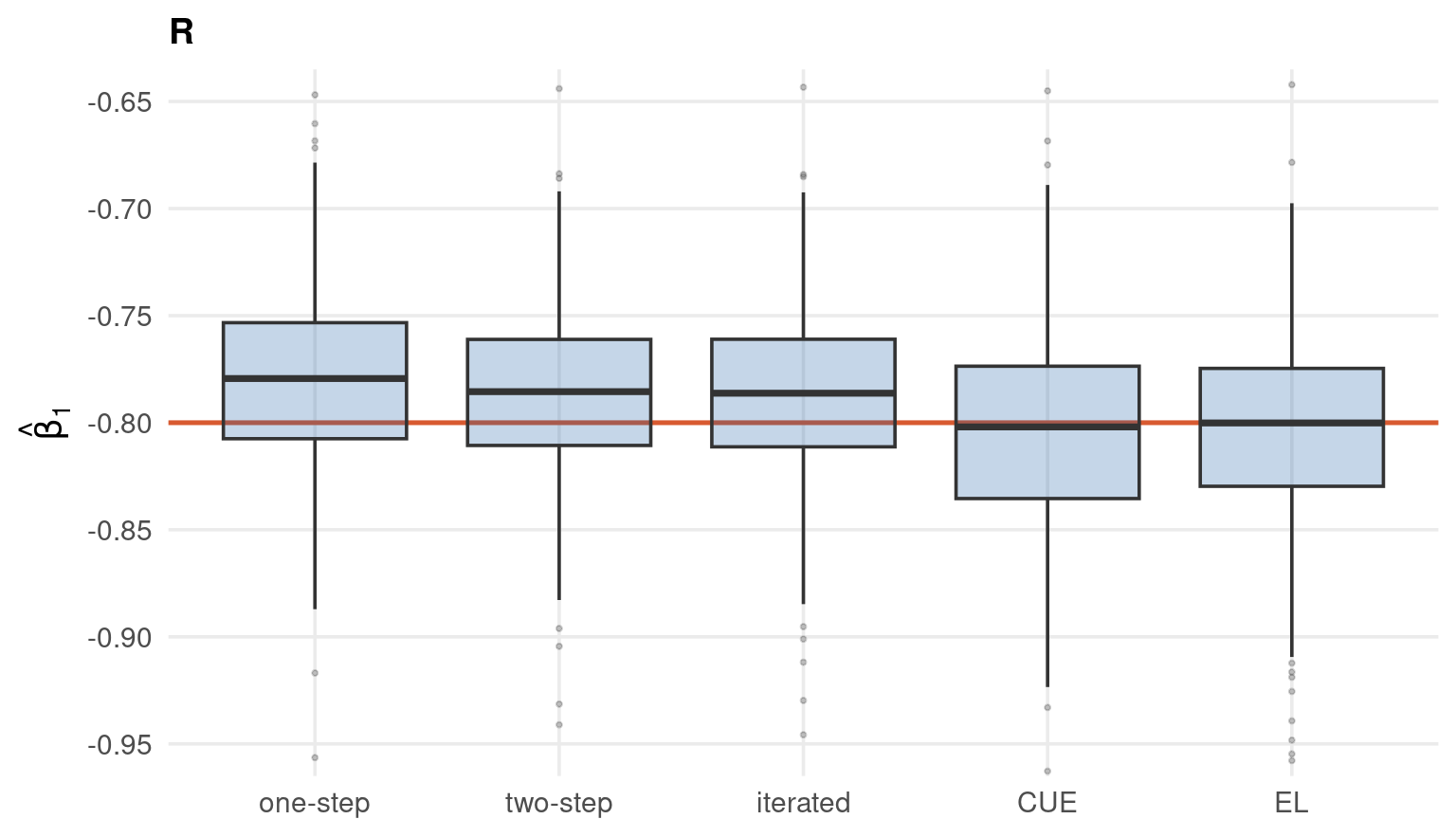
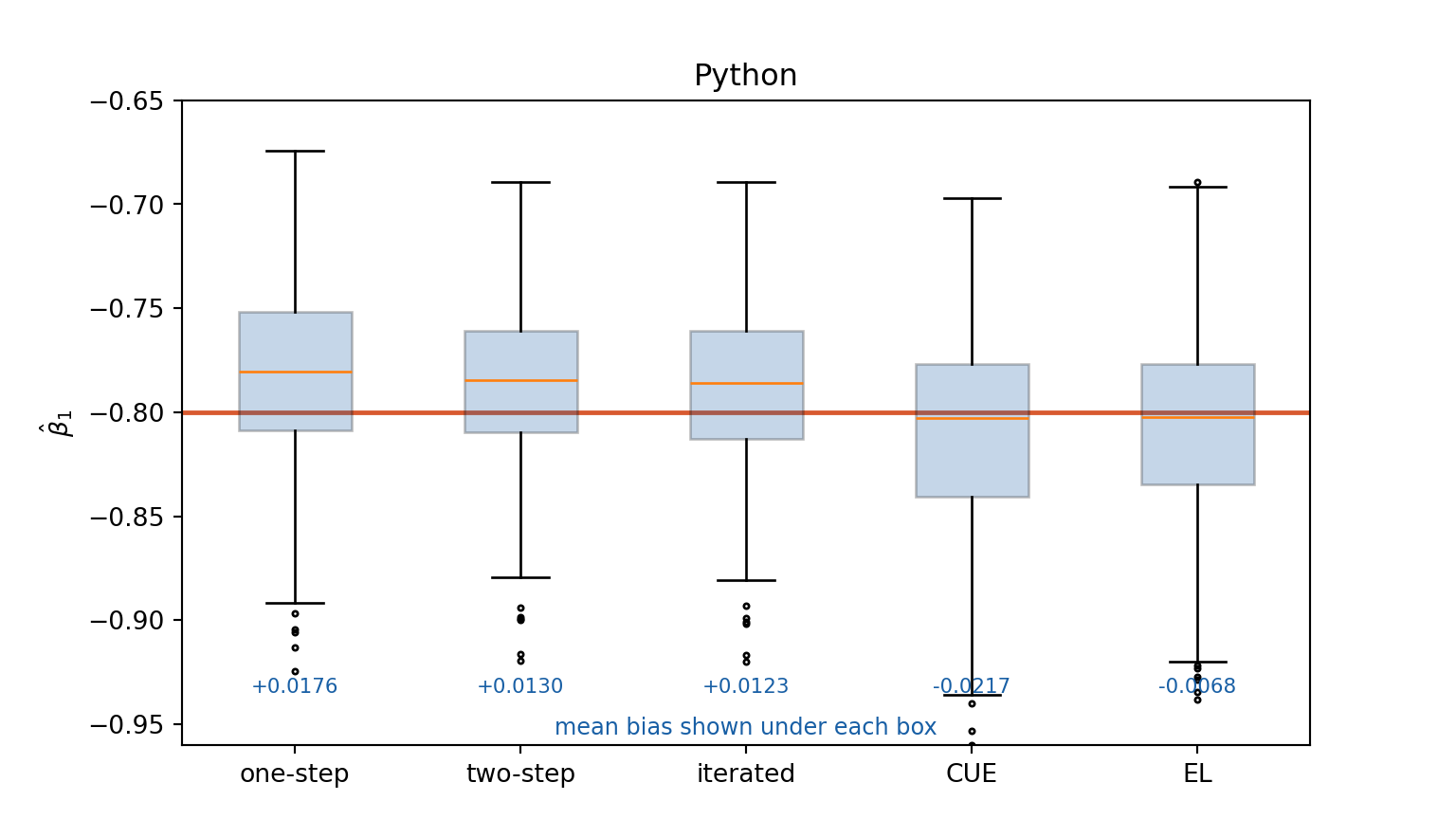
\(n = 200\), twelve moments (the six from Part 2 plus squares and cross-products of the cost shifters), 400 replications, seed 14159, 12 cores. The number reported is \(\hat\beta_1\); the truth is \(-0.8\).

Twelve moments on two hundred observations is where the \(1/n\) bias term bites. At \(n = 2000\) with six moments — the previous slide — all five estimators agreed to three decimals.

library(parallel)

gen <- function(seed, n = 200) {
  set.seed(seed)
  z1 <- rnorm(n); z2 <- rnorm(n); z3 <- rnorm(n); z4 <- rnorm(n)
  x  <- rnorm(n); v <- rnorm(n); e <- rnorm(n)
  u  <- 1.2*(0.95*v + sqrt(1 - 0.95^2)*e)
  p  <- 1 + 0.35*z1 + 0.28*z2 + 0.22*z3 + 0.18*z4 + 0.5*v
  list(q = exp(2.0 - 0.8*p + 0.4*x) + u, p = p, x = x,
       Z = cbind(1, z1, z2, z3, z4, x, z1^2, z2^2, z3^2, z4^2, z1*z2, z3*z4))
}
gmi <- function(b, D) D$Z * (D$q - exp(b[1] + b[2]*D$p + b[3]*D$x))
Qf  <- function(b, D, W) { gb <- colMeans(gmi(b, D)); as.numeric(t(gb) %*% W %*% gb) }
cuef <- function(b, D) {
  G <- gmi(b, D); gb <- colMeans(G); S <- crossprod(G)/nrow(G)
  as.numeric(t(gb) %*% solve(S + diag(1e-8, 12)) %*% gb)
}
elf <- function(b, D) el_crit_R(gmi(b, D))       # the dual, as on the previous slide

one_rep <- function(seed) {
  D  <- gen(seed)
  b1 <- optim(c(1,0,0), Qf, D = D, W = diag(12), method = "BFGS")$par
  S1 <- crossprod(gmi(b1, D))/200
  b2 <- optim(b1, Qf, D = D, W = solve(S1 + diag(1e-8, 12)), method = "BFGS")$par
  bi <- b2
  for (k in 1:8) {
    Sk <- crossprod(gmi(bi, D))/200
    bi <- optim(bi, Qf, D = D, W = solve(Sk + diag(1e-8, 12)), method = "BFGS")$par
  }
  bc <- optim(b2, cuef, D = D, method = "Nelder-Mead", control = list(maxit = 500))$par
  be <- optim(b2, elf,  D = D, method = "Nelder-Mead", control = list(maxit = 500))$par
  c(b1[2], b2[2], bi[2], bc[2], be[2])
}
out <- simplify2array(mclapply(1:400, function(r) one_rep(14159 + r), mc.cores = 12))

 estimator    bias   rmse med.bias
  one-step  0.0185 0.0476   0.0206
  two-step  0.0130 0.0432   0.0145
  iterated  0.0122 0.0435   0.0138
       CUE -0.0103 0.0658  -0.0020
        EL -0.0041 0.0481  -0.0001

import warnings; warnings.filterwarnings("ignore")   # loky shutdown chatter
from joblib import Parallel, delayed

def gen(seed, nn=200):
    r = np.random.default_rng(seed)
    z1,z2,z3,z4,x,v,e = (r.standard_normal(nn) for _ in range(7))
    u = 1.2*(0.95*v + np.sqrt(1-0.95**2)*e)
    p = 1 + 0.35*z1 + 0.28*z2 + 0.22*z3 + 0.18*z4 + 0.5*v
    Z = np.column_stack([np.ones(nn),z1,z2,z3,z4,x,z1**2,z2**2,z3**2,z4**2,z1*z2,z3*z4])
    return dict(q=np.exp(2.0 - 0.8*p + 0.4*x)+u, p=p, x=x, Z=Z)

def gmi(b, D): return D["Z"]*(D["q"] - np.exp(b[0]+b[1]*D["p"]+b[2]*D["x"]))[:,None]
def Qf(b, D, W):
    gb = gmi(b,D).mean(axis=0); return gb @ W @ gb
def cuef(b, D):
    G = gmi(b,D); gb = G.mean(axis=0); S = G.T@G/len(G)
    return gb @ np.linalg.inv(S + 1e-8*np.eye(12)) @ gb
def elf(b, D):
    G = gmi(b,D); m = G.shape[1]; lam = np.zeros(m)
    for _ in range(50):
        z = np.maximum(1 + G@lam, 1e-8)
        gr = (G/z[:,None]).sum(axis=0); H = -(G/z[:,None]**2).T@G
        try: step = np.linalg.solve(H - 1e-10*np.eye(m), gr)
        except np.linalg.LinAlgError: break
        f0 = np.sum(np.log(np.maximum(1+G@lam, 1e-12))); moved = False
        for h in range(13):
            cand = lam - step/2**h; zc = 1 + G@cand
            if zc.min() > 1e-8 and np.sum(np.log(zc)) >= f0:
                lam = cand; moved = True; break
        if not moved or np.max(np.abs(step)) < 1e-10: break
    z = 1 + G@lam
    return 1e6 if z.min() <= 1e-8 else 2*np.sum(np.log(z))

def one_rep(seed):
    D  = gen(seed)
    b1 = minimize(Qf, [1,0,0], args=(D, np.eye(12)), method="BFGS").x
    S1 = gmi(b1,D).T@gmi(b1,D)/200
    b2 = minimize(Qf, b1, args=(D, np.linalg.inv(S1+1e-8*np.eye(12))), method="BFGS").x
    bi = b2
    for _ in range(8):
        Sk = gmi(bi,D).T@gmi(bi,D)/200
        bi = minimize(Qf, bi, args=(D, np.linalg.inv(Sk+1e-8*np.eye(12))), method="BFGS").x
    bc = minimize(cuef, b2, args=(D,), method="Nelder-Mead", options=dict(maxiter=500)).x
    be = minimize(elf,  b2, args=(D,), method="Nelder-Mead", options=dict(maxiter=500)).x
    return [b1[1], b2[1], bi[1], bc[1], be[1]]

mc = np.array(Parallel(n_jobs=12)(delayed(one_rep)(14159+r) for r in range(1, 401))).T
nm = ["one-step", "two-step", "iterated", "CUE", "EL"]

fig, ax = plt.subplots(figsize=(8, 4.6))
ln = ax.axhline(-0.8, color="#D85A30", lw=1.8)
bp = ax.boxplot([mc[i] for i in range(5)], labels=nm, patch_artist=True,
                flierprops=dict(markersize=2))
for b in bp["boxes"]: b.set_facecolor("#185FA5"); b.set_alpha(0.25)
for i in range(5):
    txt = ax.text(i+1, -0.935, f"{mc[i].mean()+0.8:+.4f}", ha="center", fontsize=8,
                  color="#185FA5")
txt = ax.text(3, -0.955, "mean bias shown under each box", ha="center", fontsize=9,
              color="#185FA5")
axopts = ax.set(ylim=(-0.96, -0.65), yticks=np.arange(-0.95, -0.64, 0.05),
                ylabel=r"$\hat\beta_1$", title="Python")
plt.show()

clear all
set more off
mata:
real matrix gmi(real rowvector b, real matrix Z, real colvector q,
                real colvector p, real colvector x)
    return(Z :* (q - exp(b[1] :+ b[2]*p :+ b[3]*x)))

void Qf(todo, b, Z, q, p, x, W, val, grad, hess) {
    gb = mean(gmi(b,Z,q,p,x))
    val = -(gb*W*gb')
}
void cuef(todo, b, Z, q, p, x, dummy, val, grad, hess) {
    G = gmi(b,Z,q,p,x); gb = mean(G); S = quadcross(G,G)/rows(G)
    val = -(gb*invsym(S + 1e-8*I(12))*gb')
}
real rowvector fitW(real matrix Z, real colvector q, real colvector p,
                    real colvector x, real matrix W, real rowvector b0) {
    M = optimize_init()
    optimize_init_evaluator(M, &Qf()); optimize_init_evaluatortype(M, "d0")
    optimize_init_which(M, "max");     optimize_init_technique(M, "nm")
    optimize_init_tracelevel(M, "none"); optimize_init_nmsimplexdeltas(M, J(1,3,0.1))
    optimize_init_params(M, b0)
    optimize_init_argument(M, 1, Z); optimize_init_argument(M, 2, q)
    optimize_init_argument(M, 3, p); optimize_init_argument(M, 4, x)
    optimize_init_argument(M, 5, W)
    return(optimize(M))
}
rseed(14159)
R = 400; out = J(R, 3, .)
for (r=1; r<=R; r++) {
    n = 200
    z1=rnormal(n,1,0,1); z2=rnormal(n,1,0,1); z3=rnormal(n,1,0,1); z4=rnormal(n,1,0,1)
    x =rnormal(n,1,0,1); v =rnormal(n,1,0,1); e =rnormal(n,1,0,1)
    u = 1.2*(0.95*v + sqrt(1-0.95^2)*e)
    p = 1 :+ 0.35*z1+0.28*z2+0.22*z3+0.18*z4 + 0.5*v
    q = exp(2.0 :- 0.8*p :+ 0.4*x) + u
    Z = (J(n,1,1), z1,z2,z3,z4,x, z1:^2,z2:^2,z3:^2,z4:^2, z1:*z2, z3:*z4)
    b1 = fitW(Z,q,p,x, I(12), (1,0,0))
    G1 = gmi(b1,Z,q,p,x); S1 = quadcross(G1,G1)/n
    b2 = fitW(Z,q,p,x, invsym(S1 + 1e-8*I(12)), b1)
    bi = b2
    for (k=1; k<=8; k++) {
        Gk = gmi(bi,Z,q,p,x); Sk = quadcross(Gk,Gk)/n
        bi = fitW(Z,q,p,x, invsym(Sk + 1e-8*I(12)), bi)
    }
    C = optimize_init()
    optimize_init_evaluator(C, &cuef()); optimize_init_evaluatortype(C, "d0")
    optimize_init_which(C, "max");       optimize_init_technique(C, "nm")
    optimize_init_tracelevel(C, "none"); optimize_init_nmsimplexdeltas(C, J(1,3,0.1))
    optimize_init_params(C, b2)
    optimize_init_argument(C, 1, Z); optimize_init_argument(C, 2, q)
    optimize_init_argument(C, 3, p); optimize_init_argument(C, 4, x)
    optimize_init_argument(C, 5, 0)
    bc = optimize(C)
    out[r,] = (b1[2], b2[2], bc[2])
}
nm = ("one-step", "two-step", "CUE")
printf("%-10s%10s%10s%10s\n", "estimator", "bias", "rmse", "med.bias")
for (j=1; j<=3; j++) {
    col = out[.,j]
    printf("%-10s%10.4f%10.4f%10.4f\n", nm[j], mean(col) + 0.8,
           sqrt(mean((col :+ 0.8):^2)), 0.8 + sort(col,1)[floor(R/2)])
}
printf("\nMata has no parallel loop, so this tab runs 400 replications serially\n")
printf("and reports three estimators; R and Python add iterated GMM and EL.\n")
end

------------------------------------------------- mata (type end to exit) ----------------------------------------------
: real matrix gmi(real rowvector b, real matrix Z, real colvector q,
>                 real colvector p, real colvector x)
>     return(Z :* (q - exp(b[1] :+ b[2]*p :+ b[3]*x)))

: 
: void Qf(todo, b, Z, q, p, x, W, val, grad, hess) {
>     gb = mean(gmi(b,Z,q,p,x))
>     val = -(gb*W*gb')
> }
note: argument todo unused.
note: argument grad unused.
note: argument hess unused.

: void cuef(todo, b, Z, q, p, x, dummy, val, grad, hess) {
>     G = gmi(b,Z,q,p,x); gb = mean(G); S = quadcross(G,G)/rows(G)
>     val = -(gb*invsym(S + 1e-8*I(12))*gb')
> }
note: argument todo unused.
note: argument dummy unused.
note: argument grad unused.
note: argument hess unused.

: real rowvector fitW(real matrix Z, real colvector q, real colvector p,
>                     real colvector x, real matrix W, real rowvector b0) {
>     M = optimize_init()
>     optimize_init_evaluator(M, &Qf()); optimize_init_evaluatortype(M, "d0")
>     optimize_init_which(M, "max");     optimize_init_technique(M, "nm")
>     optimize_init_tracelevel(M, "none"); optimize_init_nmsimplexdeltas(M, J(1,3,0.1))
>     optimize_init_params(M, b0)
>     optimize_init_argument(M, 1, Z); optimize_init_argument(M, 2, q)
>     optimize_init_argument(M, 3, p); optimize_init_argument(M, 4, x)
>     optimize_init_argument(M, 5, W)
>     return(optimize(M))
> }

: rseed(14159)

: R = 400; out = J(R, 3, .)

: for (r=1; r<=R; r++) {
>     n = 200
>     z1=rnormal(n,1,0,1); z2=rnormal(n,1,0,1); z3=rnormal(n,1,0,1); z4=rnormal(n,1,0,1)
>     x =rnormal(n,1,0,1); v =rnormal(n,1,0,1); e =rnormal(n,1,0,1)
>     u = 1.2*(0.95*v + sqrt(1-0.95^2)*e)
>     p = 1 :+ 0.35*z1+0.28*z2+0.22*z3+0.18*z4 + 0.5*v
>     q = exp(2.0 :- 0.8*p :+ 0.4*x) + u
>     Z = (J(n,1,1), z1,z2,z3,z4,x, z1:^2,z2:^2,z3:^2,z4:^2, z1:*z2, z3:*z4)
>     b1 = fitW(Z,q,p,x, I(12), (1,0,0))
>     G1 = gmi(b1,Z,q,p,x); S1 = quadcross(G1,G1)/n
>     b2 = fitW(Z,q,p,x, invsym(S1 + 1e-8*I(12)), b1)
>     bi = b2
>     for (k=1; k<=8; k++) {
>         Gk = gmi(bi,Z,q,p,x); Sk = quadcross(Gk,Gk)/n
>         bi = fitW(Z,q,p,x, invsym(Sk + 1e-8*I(12)), bi)
>     }
>     C = optimize_init()
>     optimize_init_evaluator(C, &cuef()); optimize_init_evaluatortype(C, "d0")
>     optimize_init_which(C, "max");       optimize_init_technique(C, "nm")
>     optimize_init_tracelevel(C, "none"); optimize_init_nmsimplexdeltas(C, J(1,3,0.1))
>     optimize_init_params(C, b2)
>     optimize_init_argument(C, 1, Z); optimize_init_argument(C, 2, q)
>     optimize_init_argument(C, 3, p); optimize_init_argument(C, 4, x)
>     optimize_init_argument(C, 5, 0)
>     bc = optimize(C)
>     out[r,] = (b1[2], b2[2], bc[2])
> }

: nm = ("one-step", "two-step", "CUE")

: printf("%-10s%10s%10s%10s\n", "estimator", "bias", "rmse", "med.bias")
estimator       bias      rmse  med.bias

: for (j=1; j<=3; j++) {
>     col = out[.,j]
>     printf("%-10s%10.4f%10.4f%10.4f\n", nm[j], mean(col) + 0.8,
>            sqrt(mean((col :+ 0.8):^2)), 0.8 + sort(col,1)[floor(R/2)])
> }
one-step      0.0204    0.0464    0.0206
two-step      0.0144    0.0418    0.0174
CUE          -0.0056    0.0519    0.0011

: printf("\nMata has no parallel loop, so this tab runs 400 replications serially\n")

Mata has no parallel loop, so this tab runs 400 replications serially

: printf("and reports three estimators; R and Python add iterated GMM and EL.\n")
and reports three estimators; R and Python add iterated GMM and EL.

: end
------------------------------------------------------------------------------------------------------------------------

Implied Probabilities — a Free Influence Diagnostic

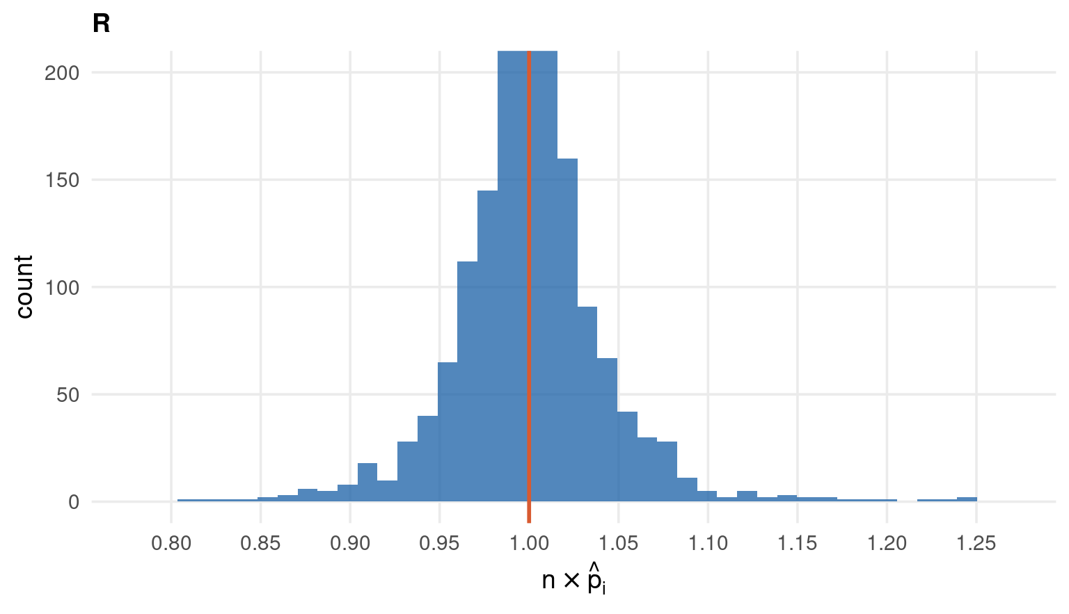
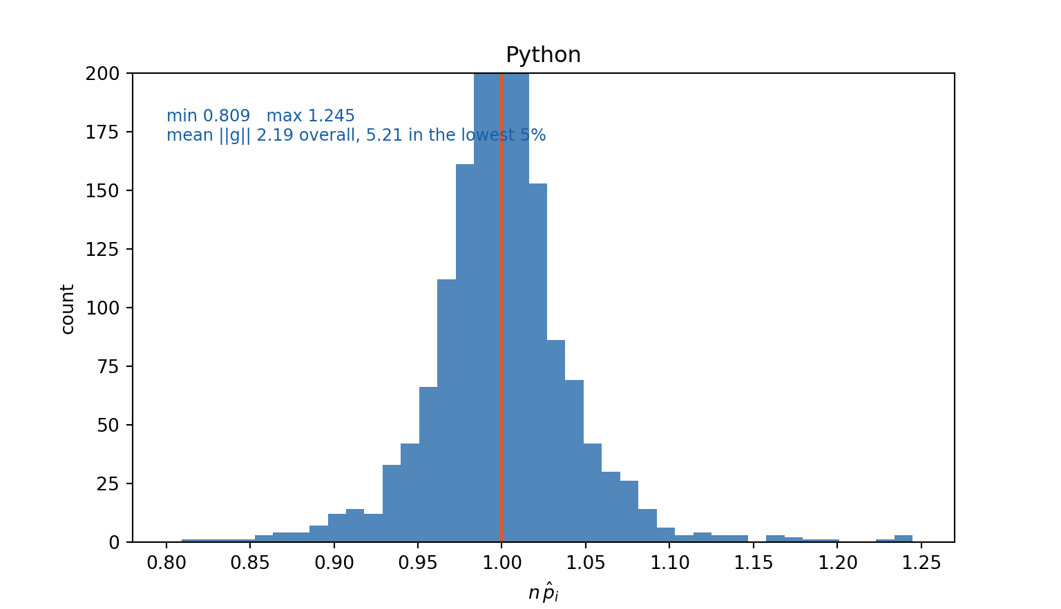
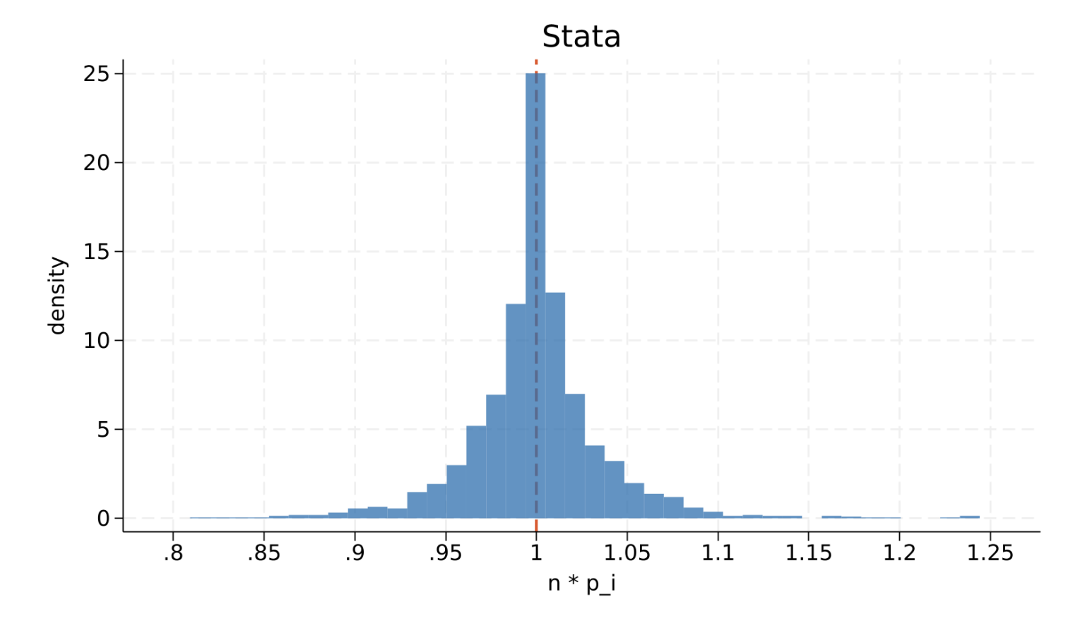
Empirical likelihood hands back the weights \(\hat p_i\) it needed in order to make the moments hold exactly. Scaled by \(n\) they centre on 1, and the distance from 1 measures how hard each observation had to be pushed.

On this sample they run from 0.81 to 1.25: no single observation is driving the result. The 5% furthest from 1 have moment vectors with norm 5.21 on average against 2.19 across the sample — EL is down-weighting exactly the observations with the largest moment contributions, which is the diagnostic you would otherwise have to build by hand.

np_i <- el$pt * nrow(d)                      # implied probabilities, scaled by n
G    <- g6(coef(el), as.matrix(d))
nrmg <- sqrt(rowSums(G^2))

cat(sprintf("n*p_i : min %.3f  max %.3f  sd %.4f\n", min(np_i), max(np_i), sd(np_i)))
cat(sprintf("mean ||g_i|| : %.2f overall, %.2f among the 5%% most down-weighted\n",
            mean(nrmg), mean(nrmg[np_i < quantile(np_i, 0.05)])))

ggplot(data.frame(np = np_i)) +
  aes(np) +
  geom_histogram(bins = 40, fill = "#185FA5", alpha = 0.75) +
  geom_vline(xintercept = 1, colour = "#D85A30", linewidth = 1) +
  coord_cartesian(xlim = c(0.78, 1.27), ylim = c(0, 200)) +
  scale_x_continuous(breaks = seq(0.8, 1.25, 0.05)) +
  labs(x = expression(n %*% hat(p)[i]), y = "count", title = "R")

n*p_i : min 0.809  max 1.245  sd 0.0375  (uniform weights would be 1)

mean ||g_i|| : 2.19 overall, 5.21 among the 5% most down-weighted

def el_weights(b):                           # recover lambda, then p_i
    G = gi(b); m = G.shape[1]; lam = np.zeros(m)
    for _ in range(60):
        z = np.maximum(1 + G @ lam, 1e-8)
        gr = (G/z[:,None]).sum(axis=0); H = -(G/z[:,None]**2).T @ G
        step = np.linalg.solve(H - 1e-10*np.eye(m), gr)
        f0 = np.sum(np.log(np.maximum(1 + G@lam, 1e-12)))
        for h in range(13):
            cand = lam - step/2**h; zc = 1 + G@cand
            if zc.min() > 1e-8 and np.sum(np.log(zc)) >= f0:
                lam = cand; break
        if np.max(np.abs(step)) < 1e-10: break
    z = 1 + G @ lam
    return 1/(z), G                          # n*p_i = 1/(1+lambda'g_i)

np_i, G = el_weights(r_el.x)
nrmg = np.sqrt((G**2).sum(axis=1))
cut  = np.quantile(np_i, 0.05)

fig, ax = plt.subplots(figsize=(8, 4.6))
hst = ax.hist(np_i, bins=40, color="#185FA5", alpha=0.75)
ln = ax.axvline(1, color="#D85A30", lw=2)
txt = ax.text(0.80, 185, f"min {np_i.min():.3f}   max {np_i.max():.3f}\n"
                         f"mean ||g|| {nrmg.mean():.2f} overall, "
                         f"{nrmg[np_i < cut].mean():.2f} in the lowest 5%",
              fontsize=9, color="#185FA5", va="top")
axopts = ax.set(xlim=(0.78, 1.27), ylim=(0, 200),
                xticks=np.arange(0.80, 1.26, 0.05),
                xlabel=r"$n\,\hat p_i$", ylabel="count", title="Python")
plt.show()

quietly import delimited "../data/moments-dgp.csv", clear
quietly destring _all, replace

mata:
q = st_data(., "q"); p = st_data(., "p"); x = st_data(., "x")
Z = (J(rows(q),1,1), st_data(., ("z1","z2","z3","z4","x")))
b = (1.9950, -0.7823, 0.3956)                 // the EL estimate
G = Z :* (q - exp(b[1] :+ b[2]*p :+ b[3]*x))
m = cols(G); lam = J(1,m,0)
for (it=1; it<=60; it++) {
    z = 1 :+ G*lam'
    z = z :* (z:>1e-8) :+ 1e-8:*(z:<=1e-8)
    gr = colsum(G :/ z); H = -quadcross(G :/ (z:^2), G)
    step = lusolve(H - 1e-10*I(m), gr')'
    if (hasmissing(step)) break
    f0 = sum(log(1 :+ G*lam'))
    for (h=0; h<=12; h++) {
        cand = lam - step/(2^h)
        zc = 1 :+ G*cand'
        if (min(zc) > 1e-8) {
            if (sum(log(zc)) >= f0) {
                lam = cand
                break
            }
        }
    }
    if (max(abs(step)) < 1e-10) break
}
npi = 1 :/ (1 :+ G*lam')                      // n * p_i
st_addvar("double", "npi")
st_store(., "npi", npi)
end

twoway (histogram npi, bin(40) fcolor("24 95 165%75") lcolor(none)),           ///
       xline(1, lcolor("216 90 48") lwidth(medthick))                          ///
       xscale(range(0.78 1.27)) xlabel(0.80(0.05)1.25)                         ///
       xtitle("n * p_i") ytitle("density")                                     ///
       legend(off) title("Stata") graphregion(color(white))

quietly graph export "../plots/moments-elweights.png", replace width(1600)

Part 4 — Simulation-Based Moments

When the Moments Have No Closed Form

• The Problem
• The Estimator
• Which Moments?

Everything so far assumed \(\bar g(\theta)\) could be written down. Plenty of structural models fail that test. The running example for this Part is stochastic volatility:

\[y_t = \exp(h_t/2)\,\varepsilon_t, \qquad h_t = \mu + \phi\,(h_{t-1} - \mu) + \sigma_\eta\,\eta_t\]

The volatility \(h_t\) is never observed. To get the likelihood you must integrate it out over the whole sample path:

\[\mathcal{L}(\theta) = \int_{\mathbb{R}^{T}} \prod_{t=1}^{T} f(y_t \mid h_t)\, f(h_t \mid h_{t-1}, \theta)\ \mathrm{d}h_1 \cdots \mathrm{d}h_T\]

A \(T = 2000\) dimensional integral. Not hard — impossible, by the usual routes.

But the model is trivial to simulate: draw \(\eta\), run the recursion, draw \(\varepsilon\), multiply. That is the whole idea of this Part.

Replace the population moment, which you cannot compute, by an average over \(S\) simulated paths of length \(T\) drawn at the candidate \(\theta\):

\[\hat\theta_{\text{SMM}} = \arg\min_\theta \ \Big(m_{\text{data}} - \bar m_S(\theta)\Big)' W \Big(m_{\text{data}} - \bar m_S(\theta)\Big)\]

\[\bar m_S(\theta) = \frac{1}{S}\sum_{s=1}^{S} m\big(y^{s}(\theta)\big)\]

Consistency needs \(T \to \infty\); \(S\) may stay fixed. The price of a finite \(S\) is a variance inflation of exactly

\[V_{\text{SMM}} = \left(1 + \frac{1}{S}\right) V_{\text{GMM}}\]

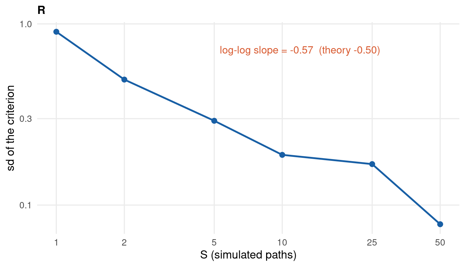
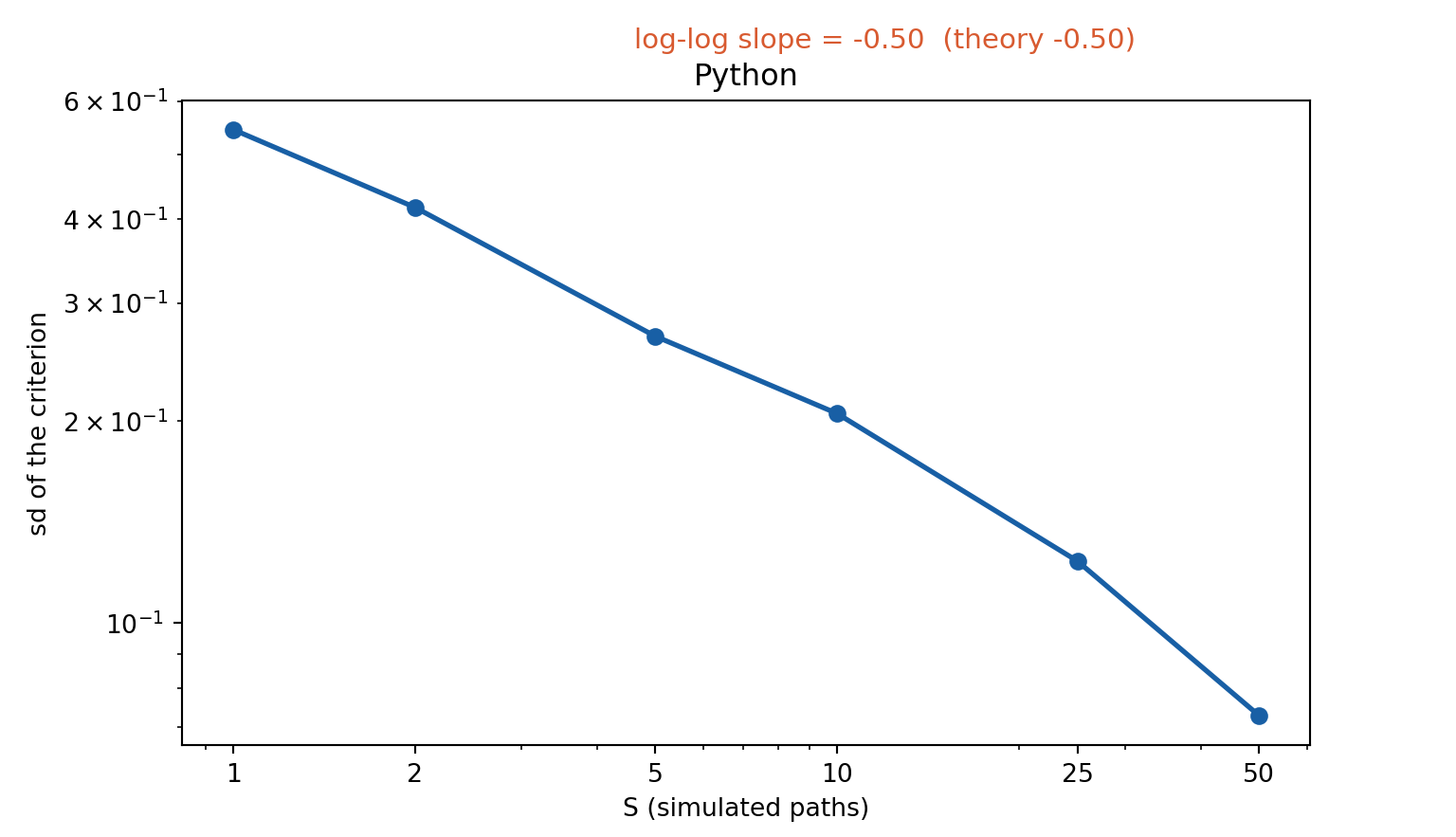
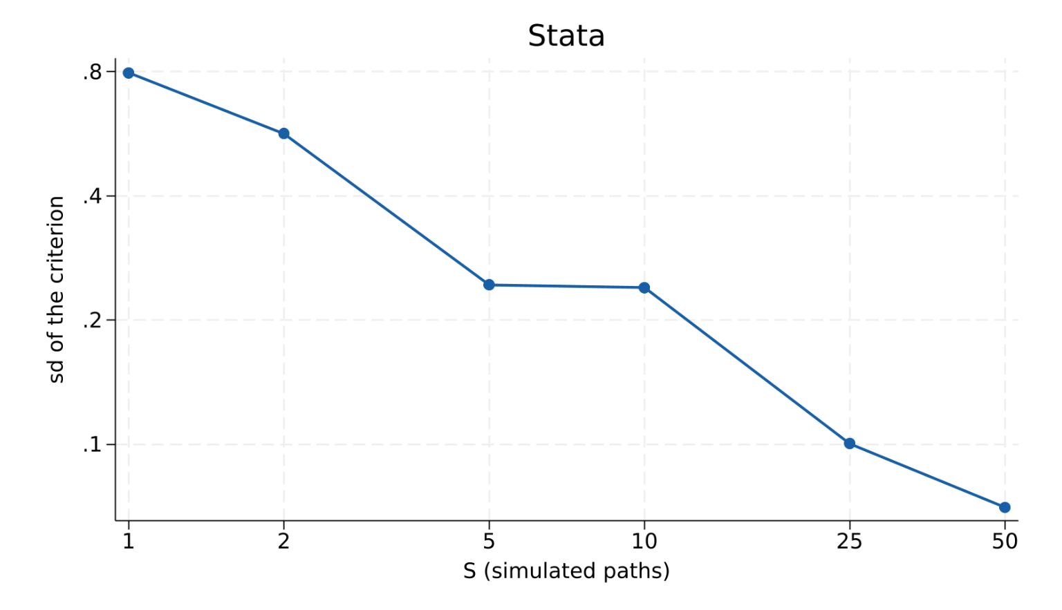
\(S = 10\) costs 10% extra variance, \(S = 1\) costs 100%. That is the entire trade-off, and it is why nobody needs \(S = 1000\).

For this model the classical choice (Andersen & Sørensen, 1996) works on \(x_t = \log y_t^2\), because taking logs turns the latent recursion into a linear one:

\[x_t = h_t + \log \varepsilon_t^2\]

an AR(1) signal plus noise. So the mean, variance and autocovariances of \(x_t\) speak directly about \((\mu, \phi, \sigma_\eta)\):

\[m(y) = \Big(\overline{x},\ \widehat{\mathrm{var}}(x),\ \widehat{\mathrm{cov}}(x_t, x_{t-1}),\ \widehat{\mathrm{cov}}(x_t, x_{t-2}),\ \widehat{\mathrm{cov}}(x_t, x_{t-5}),\ \widehat{\mathrm{cov}}(x_t, x_{t-10})\Big)\]

Six moments, three parameters — over-identified, as usual.

Common Random Numbers — the Difference Between Working and Not

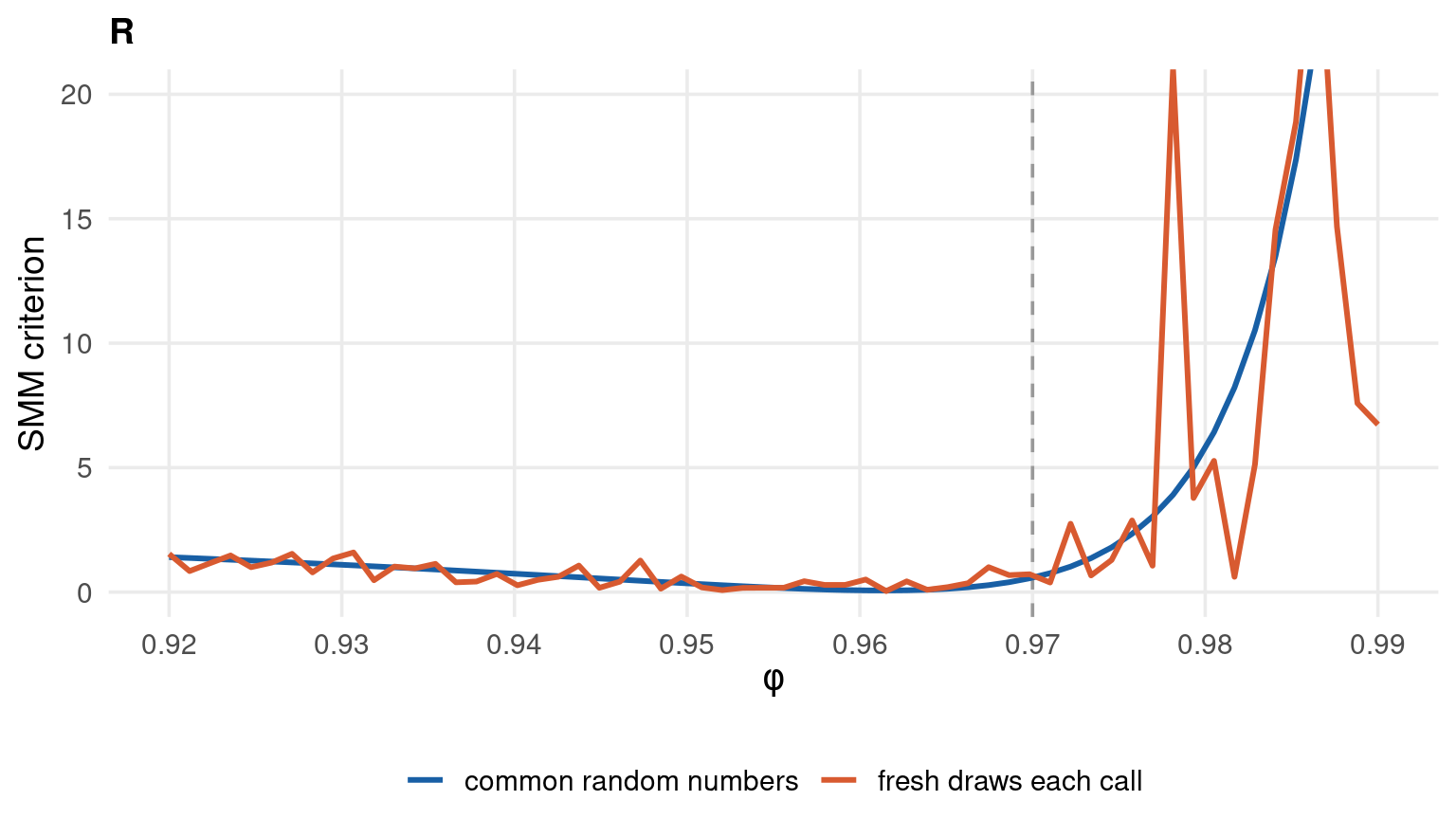
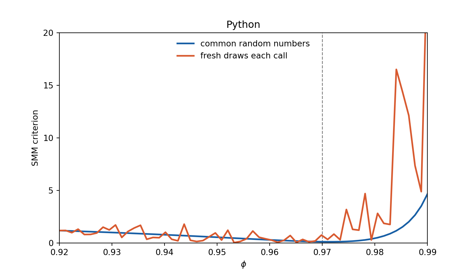
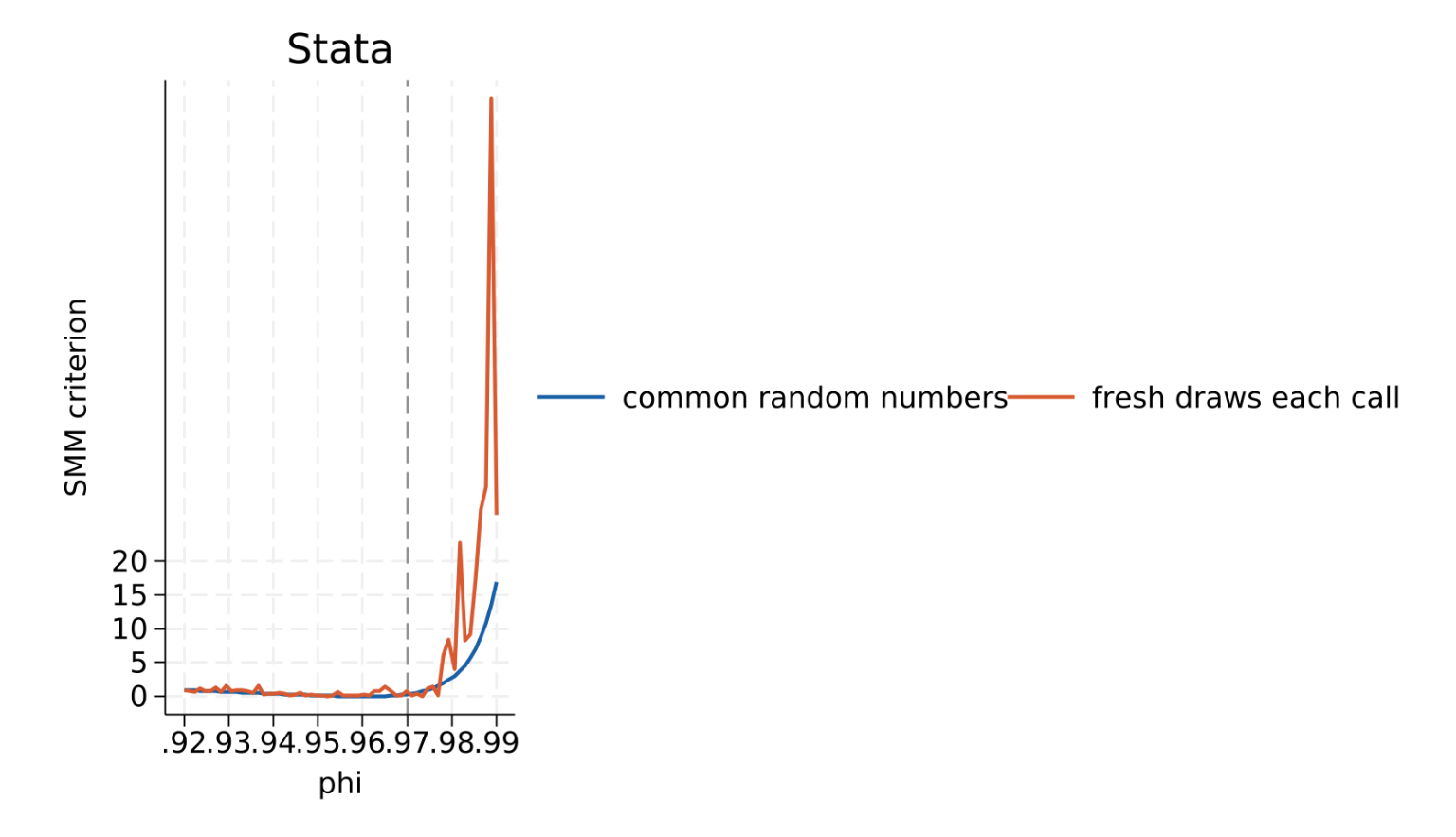
Draw fresh shocks at every trial value of \(\theta\) and the objective becomes a different random function at every point: the optimiser is chasing noise. Draw the shocks once, before the optimisation, and reuse the same \((\varepsilon, \eta)\) for every \(\theta\), and the objective becomes a smooth, deterministic function that an ordinary optimiser can minimise.

The two curves below profile the same criterion in \(\phi\), holding \(\mu = -0.40\) and \(\sigma_\eta = 0.30\) at the truth. Same model, same moments, same seed — the only difference is when the shocks are drawn.

sv <- read.csv("../data/moments-latent.csv")
Tn <- nrow(sv)

mom <- function(v) {
  x <- log(v^2 + 1e-4); n <- length(x); xc <- x - mean(x)
  lg <- function(k) sum(xc[-(1:k)] * xc[1:(n-k)]) / n
  c(mean(x), sum(xc^2)/n, lg(1), lg(2), lg(5), lg(10))
}
sim_phi <- function(phi, ep, et) {          # mu and sigma held at the truth
  h <- numeric(Tn); h[1] <- -0.40 + 0.30/sqrt(1 - phi^2) * et[1]
  for (t in 2:Tn) h[t] <- -0.40 + phi*(h[t-1] + 0.40) + 0.30*et[t]
  exp(h/2) * ep
}
m_data <- mom(sv$y)
W      <- diag(1/(abs(m_data) + 0.1)^2)
crit   <- function(v) { dd <- m_data - mom(v); as.numeric(t(dd) %*% W %*% dd) }

phis <- seq(0.92, 0.99, length.out = 60)
set.seed(14159); ep0 <- rnorm(Tn); et0 <- rnorm(Tn)     # drawn ONCE
crn <- sapply(phis, function(p) crit(sim_phi(p, ep0, et0)))
set.seed(14159)                                          # redrawn every time
fresh <- sapply(phis, function(p) crit(sim_phi(p, rnorm(Tn), rnorm(Tn))))

curves <- rbind(data.frame(phi = phis, Q = crn,   draws = "common random numbers"),
                data.frame(phi = phis, Q = fresh, draws = "fresh draws each call"))

ggplot(curves) +
  aes(phi, Q, colour = draws) +
  geom_vline(xintercept = 0.97, colour = "grey60", linetype = "dashed") +
  geom_line(linewidth = 1.05) +
  scale_colour_manual(values = c("common random numbers" = "#185FA5",
                                 "fresh draws each call" = "#D85A30")) +
  coord_cartesian(xlim = c(0.92, 0.99), ylim = c(0, 20)) +
  scale_x_continuous(breaks = seq(0.92, 0.99, 0.01)) +
  scale_y_continuous(breaks = seq(0, 20, 5)) +
  labs(x = expression(phi), y = "SMM criterion", colour = NULL, title = "R")

import numpy as np, pandas as pd, matplotlib.pyplot as plt

sv = pd.read_csv("../data/moments-latent.csv")
T  = len(sv)

def mom(v):
    x = np.log(v**2 + 1e-4); xc = x - x.mean(); n = len(x)
    lg = lambda k: (xc[k:] * xc[:n-k]).sum() / n
    return np.array([x.mean(), (xc**2).sum()/n, lg(1), lg(2), lg(5), lg(10)])

def sim_phi(phi, ep, et):                   # mu and sigma held at the truth
    h = np.empty(T); h[0] = -0.40 + 0.30/np.sqrt(1 - phi**2)*et[0]
    for t in range(1, T):
        h[t] = -0.40 + phi*(h[t-1] + 0.40) + 0.30*et[t]
    return np.exp(h/2) * ep

m_data = mom(sv.y.values)
W      = np.diag(1/(np.abs(m_data) + 0.1)**2)
crit   = lambda v: (m_data - mom(v)) @ W @ (m_data - mom(v))

phis = np.linspace(0.92, 0.99, 60)
rng  = np.random.default_rng(14159)
ep0, et0 = rng.standard_normal(T), rng.standard_normal(T)      # drawn ONCE
crn = [crit(sim_phi(p, ep0, et0)) for p in phis]
rng = np.random.default_rng(14159)                              # redrawn each call
fresh = [crit(sim_phi(p, rng.standard_normal(T), rng.standard_normal(T)))
         for p in phis]

fig, ax = plt.subplots(figsize = (8, 4.6))
ln = ax.axvline(0.97, color = "grey", ls = "--", lw = 1)
ln = ax.plot(phis, crn,   color = "#185FA5", lw = 2, label = "common random numbers")
ln = ax.plot(phis, fresh, color = "#D85A30", lw = 2, label = "fresh draws each call")
leg = ax.legend(loc = "upper center", frameon = False)
axopts = ax.set(xlim = (0.92, 0.99), ylim = (0, 20),
                xticks = np.arange(0.92, 0.991, 0.01),
                yticks = range(0, 21, 5),
                xlabel = r"$\phi$", ylabel = "SMM criterion", title = "Python")
plt.show()

quietly import delimited "../data/moments-latent.csv", clear
quietly destring _all, replace

mata:
real rowvector mom(real colvector v) {
    x = log(v:^2 :+ 1e-4); n = rows(x); xc = x :- mean(x)
    return((mean(x), sum(xc:^2)/n,
            sum(xc[2::n]:*xc[1::n-1])/n,  sum(xc[3::n]:*xc[1::n-2])/n,
            sum(xc[6::n]:*xc[1::n-5])/n,  sum(xc[11::n]:*xc[1::n-10])/n))
}
real colvector sim_phi(real scalar phi, real colvector ep, real colvector et) {
    T = rows(ep); h = J(T,1,0)
    h[1] = -0.40 + 0.30/sqrt(1-phi^2)*et[1]
    for (t=2; t<=T; t++) h[t] = -0.40 + phi*(h[t-1]+0.40) + 0.30*et[t]
    return(exp(h:/2) :* ep)
}
y = st_data(., "y"); T = rows(y)
mdata = mom(y); W = diag(1:/(abs(mdata):+0.1):^2)

rseed(14159); ep0 = rnormal(T,1,0,1); et0 = rnormal(T,1,0,1)   // drawn ONCE
out = J(60, 3, .)
for (i=1; i<=60; i++) {
    phi = 0.92 + (i-1)*(0.99-0.92)/59
    d1 = mdata - mom(sim_phi(phi, ep0, et0))
    out[i,1] = phi; out[i,2] = d1*W*d1'
}
rseed(14159)
for (i=1; i<=60; i++) {                                        // redrawn each call
    phi = 0.92 + (i-1)*(0.99-0.92)/59
    d2 = mdata - mom(sim_phi(phi, rnormal(T,1,0,1), rnormal(T,1,0,1)))
    out[i,3] = d2*W*d2'
}
end

preserve
clear
quietly set obs 60
quietly generate double phi   = .
quietly generate double crn   = .
quietly generate double fresh = .
mata: st_store(., ("phi","crn","fresh"), out)

twoway (line crn phi,   lcolor("24 95 165") lwidth(medthick))                  ///
       (line fresh phi, lcolor("216 90 48") lwidth(medthick)),                 ///
       xline(0.97, lcolor(gs9) lpattern(dash))                                 ///
       xscale(range(0.92 0.99)) yscale(range(0 20))                            ///
       xlabel(0.92(0.01)0.99) ylabel(0(5)20)                                   ///
       xtitle("phi") ytitle("SMM criterion")                                   ///
       legend(order(1 "common random numbers" 2 "fresh draws each call")       ///
              rows(1))                                                         ///
       title("Stata") graphregion(color(white))

quietly graph export "../plots/moments-crn.png", replace width(1600)
restore

SMM on a Model Whose Truth We Know

\(S = 10\) simulated paths, common random numbers, Nelder–Mead. The standard errors use the \((1 + 1/S)\) inflation, a Newey–West estimate of the data moments’ long-run variance, and a numerical Jacobian of the binding function.

The three tabs will not agree to four decimals, and that is correct. R, NumPy and Mata have different random number generators, so each language draws a different set of \((\varepsilon, \eta)\) and estimates a different realisation of the SMM criterion. What must agree — and does, exactly — is the data-side input: all three report the same six sample moments. Compare the conclusions, not the digits.

Read the three tabs together and the pattern is clear: \(\phi\) and \(\sigma_\eta\) are pinned down tightly and consistently, while \(\mu\) comes out below the truth in all three languages and carries by far the largest standard error. That is not a bug in any one of them. \(\mu\) is the mean of a latent process with \(\phi = 0.97\), so the effective number of independent observations about its level is roughly

\[T\,\frac{1 - \phi}{1 + \phi} \approx 2000 \times \frac{0.03}{1.97} \approx 30\]

Thirty, not two thousand. A level parameter estimated off thirty effective observations is exactly as imprecise as the standard errors say.

Bandwidth matters here, and the automatic rule fails. The moment contributions inherit the persistence of \(h_t\), so their autocovariances die out over roughly \(1/(1-\phi) \approx 33\) lags. The usual Newey–West plug-in rule \(4(T/100)^{2/9}\) suggests a bandwidth of 8 — at which the estimated long-run variance of the first moment is 42% too small and every \(t\)-ratio is correspondingly too large. These tabs use \(L = 100\), past the point where the estimate stops moving. Part 5 revisits this with real data.

Why the code optimises atanh(phi) and log(sigma)

The problem. Nelder–Mead and BFGS are unconstrained optimisers, but this model needs \(|\phi| < 1\) and \(\sigma_\eta > 0\). A trial step to \(\phi = 1.04\) makes \(\sigma/\sqrt{1-\phi^2}\) the square root of a negative number; a step to \(\sigma = -0.1\) simulates a process that does not exist. The criterion returns NaN, the simplex collapses around the bad vertex, and the run either stops early or reports a boundary value as if it were an estimate.

The fix. Do not add constraints — change coordinates, so that every real number is a legal parameter. Optimise \(\psi\), report \(\theta = f(\psi)\):

• \(\sigma > 0\)  →  optimise \(\log\sigma\), invert with \(\exp\)
• \(|\phi| < 1\)  →  optimise \(\operatorname{atanh}\phi\), invert with \(\tanh\)
• \(0 < p < 1\)  →  optimise \(\operatorname{logit} p\), invert with the logistic — this is how the GARCH \(\alpha\) is handled on the indirect-inference slide
• \(a < \theta < b\)  →  logit of \((\theta-a)/(b-a)\); weights on a simplex → softmax

The price, and where the code pays it. The optimiser’s curvature is in \(\psi\) units, so the standard errors must be mapped back by the delta method. With \(J = \partial\theta/\partial\psi\),

\[V_\theta = J\,V_\psi\,J', \qquad J = \operatorname{diag}\big(1,\ 1-\hat\phi^{\,2},\ \hat\sigma\big)\]

which is exactly the line Jn <- diag(c(1, 1 - tanh(par[2])^2, exp(par[3]))) in all three tabs. Here it is applied to the Jacobian of the binding function rather than to \(V\) — Gn <- Gj %*% solve(Jn) puts \(G\) into natural units, so the variance comes out on the natural scale directly. The two are the same chain rule.

One caution. The sampling distribution is closer to symmetric in \(\psi\) than in \(\theta\). For \(\hat\phi\) near one, build the interval on the optimiser scale and transform the two endpoints — do not use \(\hat\phi \pm 1.96\,\mathrm{se}_\phi\), which can hand you an interval containing values above one.

set.seed(14159)
S <- 10
eps <- matrix(rnorm(Tn*S), Tn, S)          # common random numbers, drawn once
eta <- matrix(rnorm(Tn*S), Tn, S)

# par = (mu, atanh(phi), log(sigma)) on the unconstrained scale - see the popup above
sim_sv <- function(par, s) {
  mu <- par[1]; phi <- tanh(par[2]); sig <- exp(par[3])
  h <- numeric(Tn); h[1] <- mu + sig/sqrt(1 - phi^2)*eta[1, s]
  for (t in 2:Tn) h[t] <- mu + phi*(h[t-1] - mu) + sig*eta[t, s]
  exp(h/2) * eps[, s]
}
msim <- function(par) rowMeans(sapply(1:S, function(s) mom(sim_sv(par, s))))
obj  <- function(par) { dd <- m_data - msim(par); as.numeric(t(dd) %*% W %*% dd) }

fit <- optim(c(-0.2, atanh(0.90), log(0.40)), obj, method = "Nelder-Mead",
             control = list(maxit = 600, reltol = 1e-10))
est <- c(fit$par[1], tanh(fit$par[2]), exp(fit$par[3]))

# --- standard errors -------------------------------------------------------
contrib <- function(v) {                   # T x 6 per-period contributions
  x <- log(v^2 + 1e-4); n <- length(x); xc <- x - mean(x)
  lg <- function(k) c(rep(0, k), xc[1:(n-k)]) * xc
  cbind(x, xc^2, lg(1), lg(2), lg(5), lg(10))
}
gc_ <- contrib(sv$y); gc_ <- sweep(gc_, 2, colMeans(gc_))
L <- 100; Om <- crossprod(gc_)/Tn                    # Newey-West, long bandwidth
for (j in 1:L) {
  G0 <- crossprod(gc_[-(1:j), ], gc_[1:(Tn-j), ])/Tn
  Om <- Om + (1 - j/(L+1)) * (G0 + t(G0))
}
Gj <- sapply(1:3, function(k) {                      # numerical Jacobian
  h <- 1e-4*max(1, abs(fit$par[k])); pp <- pm <- fit$par
  pp[k] <- pp[k] + h; pm[k] <- pm[k] - h
  (msim(pp) - msim(pm)) / (2*h)
})
Jn <- diag(c(1, 1 - tanh(fit$par[2])^2, exp(fit$par[3])))   # chain rule
Gn <- Gj %*% solve(Jn)
V  <- (1 + 1/S) * solve(t(Gn) %*% solve(Om) %*% Gn) / Tn
se <- sqrt(diag(V))

data moments : -1.9375  5.6843  1.1527  0.9542  0.9417  0.7624

                  mu       phi     sigma

SMM          -0.6213    0.9568    0.3243

std.err       0.1662    0.0223    0.0819

truth        -0.4000    0.9700    0.3000

t vs true      -1.33     -0.59      0.30

S = 10, 138 criterion evaluations, 0.7 seconds

import time
from scipy.optimize import minimize

rng = np.random.default_rng(14159)
S = 10
eps = rng.standard_normal((T, S))          # common random numbers, drawn once
eta = rng.standard_normal((T, S))

# par = (mu, arctanh(phi), log(sigma)) on the unconstrained scale - see the popup above
def sim_sv(par, s):
    mu, phi, sig = par[0], np.tanh(par[1]), np.exp(par[2])
    h = np.empty(T); h[0] = mu + sig/np.sqrt(1 - phi**2)*eta[0, s]
    for t in range(1, T):
        h[t] = mu + phi*(h[t-1] - mu) + sig*eta[t, s]
    return np.exp(h/2) * eps[:, s]

msim = lambda par: np.mean([mom(sim_sv(par, s)) for s in range(S)], axis = 0)
obj  = lambda par: (m_data - msim(par)) @ W @ (m_data - msim(par))

t0 = time.time()
r = minimize(obj, [-0.2, np.arctanh(0.90), np.log(0.40)], method = "Nelder-Mead",
             options = dict(maxiter = 600, fatol = 1e-10, xatol = 1e-8))
secs = time.time() - t0
est = np.array([r.x[0], np.tanh(r.x[1]), np.exp(r.x[2])])

def contrib(v):                            # T x 6 per-period contributions
    x = np.log(v**2 + 1e-4); xc = x - x.mean(); n = len(x)
    cols = [x, xc**2]
    for k in (1, 2, 5, 10):
        c = np.zeros(n); c[k:] = xc[k:]*xc[:n-k]
        cols.append(c)
    return np.column_stack(cols)

g = contrib(sv.y.values); g = g - g.mean(axis = 0)
L = 100; Om = g.T @ g / T                            # Newey-West, long bandwidth
for j in range(1, L+1):
    G0 = g[j:].T @ g[:T-j] / T
    Om = Om + (1 - j/(L+1))*(G0 + G0.T)
Gj = np.column_stack([                               # numerical Jacobian
    (msim(np.where(np.arange(3) == k, r.x + 1e-4*np.maximum(1, np.abs(r.x)), r.x))
     - msim(np.where(np.arange(3) == k, r.x - 1e-4*np.maximum(1, np.abs(r.x)), r.x)))
    / (2*1e-4*max(1, abs(r.x[k]))) for k in range(3)])
Jn = np.diag([1, 1 - np.tanh(r.x[1])**2, np.exp(r.x[2])])    # chain rule
Gn = Gj @ np.linalg.inv(Jn)
V  = (1 + 1/S) * np.linalg.inv(Gn.T @ np.linalg.inv(Om) @ Gn) / T
se = np.sqrt(np.diag(V))
tr = np.array([-0.40, 0.97, 0.30])

out = ("data moments : " + " ".join(f"{v:7.4f}" for v in m_data) + "\n\n"
       + f"{'':<10}{'mu':>9}{'phi':>9}{'sigma':>9}\n"
       + f"{'SMM':<10}" + "".join(f"{v:9.4f}" for v in est) + "\n"
       + f"{'std.err':<10}" + "".join(f"{v:9.4f}" for v in se) + "\n"
       + f"{'truth':<10}" + "".join(f"{v:9.4f}" for v in tr) + "\n"
       + f"{'t vs true':<10}" + "".join(f"{v:9.2f}" for v in (est-tr)/se) + "\n"
       + f"\nS = {S}, {r.nfev} criterion evaluations, {secs:.1f} seconds")
import sys; nch = sys.stdout.write(out + "\n"); sys.stdout.flush()

data moments : -1.9375  5.6843  1.1527  0.9542  0.9417  0.7624

                 mu      phi    sigma
SMM         -0.7012   0.9626   0.3099
std.err      0.1569   0.0204   0.0779
truth       -0.4000   0.9700   0.3000
t vs true     -1.92    -0.36     0.13

S = 10, 312 criterion evaluations, 5.4 seconds

quietly import delimited "../data/moments-latent.csv", clear
quietly destring _all, replace

mata:
real matrix contrib(real colvector v) {          // T x 6 contributions
    x = log(v:^2 :+ 1e-4); n = rows(x); xc = x :- mean(x)
    C = J(n, 6, 0); C[.,1] = x; C[.,2] = xc:^2
    lags = (1,2,5,10)
    for (j=1; j<=4; j++) {
        k = lags[j]; col = J(n,1,0)
        col[k+1::n] = xc[k+1::n] :* xc[1::n-k]
        C[.,2+j] = col
    }
    return(C)
}
real rowvector mom(real colvector v) return(mean(contrib(v)))
real colvector sim_sv(real rowvector par, real colvector ep, real colvector et) {
    // unconstrained scale - see the reparameterisation popup (Part 4, SMM slide)
    mu = par[1]; phi = tanh(par[2]); sig = exp(par[3]); T = rows(ep)
    h = J(T,1,0); h[1] = mu + sig/sqrt(1-phi^2)*et[1]
    for (t=2; t<=T; t++) h[t] = mu + phi*(h[t-1]-mu) + sig*et[t]
    return(exp(h:/2) :* ep)
}
real rowvector msim(real rowvector par, real matrix EP, real matrix ET) {
    S = cols(EP); ms = J(1,6,0)
    for (s=1; s<=S; s++) ms = ms + mom(sim_sv(par, EP[.,s], ET[.,s]))
    return(ms/S)
}
void smmobj(todo, par, EP, ET, mdata, W, val, grad, hess) {
    d = mdata - msim(par, EP, ET)
    val = -(d*W*d')                              // optimize() maximises
}
y = st_data(., "y"); T = rows(y)
rseed(14159); S = 10
EP = rnormal(T,S,0,1); ET = rnormal(T,S,0,1)     // common random numbers
mdata = mom(y); W = diag(1:/(abs(mdata):+0.1):^2)

M = optimize_init()
optimize_init_evaluator(M, &smmobj());  optimize_init_evaluatortype(M, "d0")
optimize_init_which(M, "max");          optimize_init_technique(M, "nm")
optimize_init_tracelevel(M, "none");    optimize_init_nmsimplexdeltas(M, J(1,3,0.2))
optimize_init_params(M, (-0.2, atanh(0.90), log(0.40)))
optimize_init_argument(M, 1, EP);    optimize_init_argument(M, 2, ET)
optimize_init_argument(M, 3, mdata); optimize_init_argument(M, 4, W)
p = optimize(M)
est = (p[1], tanh(p[2]), exp(p[3]))

g = contrib(y); g = g :- mean(g)
L = 100; Om = quadcross(g,g)/T                   // Newey-West, long bandwidth
for (j=1; j<=L; j++) {
    G0 = quadcross(g[j+1::T,], g[1::T-j,])/T
    Om = Om + (1-j/(L+1))*(G0 + G0')
}
G = J(6,3,0)                                     // numerical Jacobian
for (k=1; k<=3; k++) {
    hh = 1e-4*max((1, abs(p[k]))); pp = p; pm = p
    pp[k] = pp[k]+hh; pm[k] = pm[k]-hh
    G[.,k] = ((msim(pp,EP,ET) - msim(pm,EP,ET))/(2*hh))'
}
Jn = diag((1, 1-tanh(p[2])^2, exp(p[3])))        // chain rule
Gn = G * luinv(Jn)
V  = (1+1/S) * luinv(Gn' * luinv(Om) * Gn) / T
se = sqrt(diagonal(V))'
tr = (-0.40, 0.97, 0.30)

printf("data moments : %7.4f %7.4f %7.4f %7.4f %7.4f %7.4f\n",
       mdata[1],mdata[2],mdata[3],mdata[4],mdata[5],mdata[6])
printf("\n%10s%9s%9s%9s\n", "", "mu", "phi", "sigma")
printf("%-10s%9.4f%9.4f%9.4f\n", "SMM",     est[1], est[2], est[3])
printf("%-10s%9.4f%9.4f%9.4f\n", "std.err", se[1],  se[2],  se[3])
printf("%-10s%9.4f%9.4f%9.4f\n", "truth",   tr[1],  tr[2],  tr[3])
printf("%-10s%9.2f%9.2f%9.2f\n", "t vs true",
       (est[1]-tr[1])/se[1], (est[2]-tr[2])/se[2], (est[3]-tr[3])/se[3])
printf("\nS = %f simulated paths\n", S)
end

------------------------------------------------- mata (type end to exit) ----------------------------------------------
: real matrix contrib(real colvector v) {          // T x 6 contributions
>     x = log(v:^2 :+ 1e-4); n = rows(x); xc = x :- mean(x)
>     C = J(n, 6, 0); C[.,1] = x; C[.,2] = xc:^2
>     lags = (1,2,5,10)
>     for (j=1; j<=4; j++) {
>         k = lags[j]; col = J(n,1,0)
>         col[k+1::n] = xc[k+1::n] :* xc[1::n-k]
>         C[.,2+j] = col
>     }
>     return(C)
> }

: real rowvector mom(real colvector v) return(mean(contrib(v)))

: real colvector sim_sv(real rowvector par, real colvector ep, real colvector et) {
>     // unconstrained scale - see the reparameterisation popup (Part 4, SMM slide)
>     mu = par[1]; phi = tanh(par[2]); sig = exp(par[3]); T = rows(ep)
>     h = J(T,1,0); h[1] = mu + sig/sqrt(1-phi^2)*et[1]
>     for (t=2; t<=T; t++) h[t] = mu + phi*(h[t-1]-mu) + sig*et[t]
>     return(exp(h:/2) :* ep)
> }

: real rowvector msim(real rowvector par, real matrix EP, real matrix ET) {
>     S = cols(EP); ms = J(1,6,0)
>     for (s=1; s<=S; s++) ms = ms + mom(sim_sv(par, EP[.,s], ET[.,s]))
>     return(ms/S)
> }

: void smmobj(todo, par, EP, ET, mdata, W, val, grad, hess) {
>     d = mdata - msim(par, EP, ET)
>     val = -(d*W*d')                              // optimize() maximises
> }
note: argument todo unused.
note: argument grad unused.
note: argument hess unused.

: y = st_data(., "y"); T = rows(y)

: rseed(14159); S = 10

: EP = rnormal(T,S,0,1); ET = rnormal(T,S,0,1)     // common random numbers

: mdata = mom(y); W = diag(1:/(abs(mdata):+0.1):^2)

: 
: M = optimize_init()

: optimize_init_evaluator(M, &smmobj());  optimize_init_evaluatortype(M, "d0")

: optimize_init_which(M, "max");          optimize_init_technique(M, "nm")

: optimize_init_tracelevel(M, "none");    optimize_init_nmsimplexdeltas(M, J(1,3,0.2))

: optimize_init_params(M, (-0.2, atanh(0.90), log(0.40)))

: optimize_init_argument(M, 1, EP);    optimize_init_argument(M, 2, ET)

: optimize_init_argument(M, 3, mdata); optimize_init_argument(M, 4, W)

: p = optimize(M)

: est = (p[1], tanh(p[2]), exp(p[3]))

: 
: g = contrib(y); g = g :- mean(g)

: L = 100; Om = quadcross(g,g)/T                   // Newey-West, long bandwidth

: for (j=1; j<=L; j++) {
>     G0 = quadcross(g[j+1::T,], g[1::T-j,])/T
>     Om = Om + (1-j/(L+1))*(G0 + G0')
> }

: G = J(6,3,0)                                     // numerical Jacobian

: for (k=1; k<=3; k++) {
>     hh = 1e-4*max((1, abs(p[k]))); pp = p; pm = p
>     pp[k] = pp[k]+hh; pm[k] = pm[k]-hh
>     G[.,k] = ((msim(pp,EP,ET) - msim(pm,EP,ET))/(2*hh))'
> }

: Jn = diag((1, 1-tanh(p[2])^2, exp(p[3])))        // chain rule

: Gn = G * luinv(Jn)

: V  = (1+1/S) * luinv(Gn' * luinv(Om) * Gn) / T

: se = sqrt(diagonal(V))'

: tr = (-0.40, 0.97, 0.30)

: 
: printf("data moments : %7.4f %7.4f %7.4f %7.4f %7.4f %7.4f\n",
>        mdata[1],mdata[2],mdata[3],mdata[4],mdata[5],mdata[6])
data moments : -1.9375  5.6843  1.1527  0.9542  0.9417  0.7624

: printf("\n%10s%9s%9s%9s\n", "", "mu", "phi", "sigma")

                 mu      phi    sigma

: printf("%-10s%9.4f%9.4f%9.4f\n", "SMM",     est[1], est[2], est[3])
SMM         -0.7499   0.9638   0.2975

: printf("%-10s%9.4f%9.4f%9.4f\n", "std.err", se[1],  se[2],  se[3])
std.err      0.1549   0.0213   0.0792

: printf("%-10s%9.4f%9.4f%9.4f\n", "truth",   tr[1],  tr[2],  tr[3])
truth       -0.4000   0.9700   0.3000

: printf("%-10s%9.2f%9.2f%9.2f\n", "t vs true",
>        (est[1]-tr[1])/se[1], (est[2]-tr[2])/se[2], (est[3]-tr[3])/se[3])
t vs true     -2.26    -0.29    -0.03

: printf("\nS = %f simulated paths\n", S)

S = 10 simulated paths

: end
------------------------------------------------------------------------------------------------------------------------

Indirect Inference — Let a Wrong Model Do the Measuring

• The Idea
• The Auxiliary Here
• Three Flavours

Choosing six moments by hand was a judgement call. Indirect inference replaces that judgement with an auxiliary model: something misspecified but easy to estimate, whose parameters are used as the statistics to match.

Fit the auxiliary to the real data, giving \(\hat\beta\). For a candidate \(\theta\), simulate from the structural model and fit the same auxiliary to the simulated data, giving the binding function \(b(\theta)\):

\[\hat\theta_{\text{II}} = \arg\min_\theta \big(\hat\beta - b_S(\theta)\big)' W \big(\hat\beta - b_S(\theta)\big)\]

The auxiliary model does not have to be true. It only has to be sensitive to \(\theta\) — a lens, not a description.

For stochastic volatility the natural lens is GARCH(1,1), which is misspecified — volatility here is driven by its own shock, not by past squared returns — but responds sharply to persistence and to the volatility of volatility:

\[\sigma_t^2 = \omega + \alpha\, y_{t-1}^2 + \beta\, \sigma_{t-1}^2\]

Three auxiliary parameters \((\omega, \alpha, \beta)\) for three structural parameters \((\mu, \phi, \sigma_\eta)\): exactly identified, so at the optimum the binding function reproduces \(\hat\beta\) almost exactly.

Fitted by Gaussian QMLE, hand-coded identically in all three languages so the lens is the same everywhere. On the data it gives

\[\hat\omega = 0.0221, \qquad \hat\alpha = 0.181, \qquad \hat\beta = 0.808\]

The distance can be measured in three places, all asymptotically equivalent:

• Wald — match the auxiliary parameters, as above. Simplest, and what the code does
• LM / score — match the auxiliary score evaluated at \(\hat\beta\) on simulated data; no inner optimisation per simulation, so much cheaper
• LR — match the auxiliary likelihood itself

The score version is what Gallant & Tauchen (1996) call the efficient method of moments: with an auxiliary rich enough to nest the true density, EMM attains the ML efficiency bound. The cost is choosing that auxiliary well — usually a semi-nonparametric (SNP) density.

Indirect Inference — Code

\(S = 2\) simulated paths. Every criterion evaluation now costs \(S\) full QMLE fits of the auxiliary model, which is why this is the expensive estimator in the deck — and why the timings are reported.

garch_ll <- function(p, v) {                 # Gaussian QMLE, transformed params
  # unconstrained scale - see the reparameterisation popup (Part 4, SMM slide)
  om <- exp(p[1]); al <- 1/(1 + exp(-p[2])); be <- (1 - al)/(1 + exp(-p[3]))
  n <- length(v); s2 <- numeric(n); s2[1] <- var(v)
  for (t in 2:n) s2[t] <- om + al*v[t-1]^2 + be*s2[t-1]
  0.5*sum(log(s2) + v^2/s2)
}
garch_fit <- function(v) {
  o  <- optim(c(log(0.05), 0, 0), garch_ll, v = v, method = "Nelder-Mead",
              control = list(maxit = 400, reltol = 1e-8))
  al <- 1/(1 + exp(-o$par[2])); be <- (1 - al)/(1 + exp(-o$par[3]))
  c(exp(o$par[1]), al, be)
}

b_data <- garch_fit(sv$y)                    # the auxiliary on the real data
Wii    <- diag(1/b_data^2)

set.seed(14159); Sii <- 2
epi <- matrix(rnorm(Tn*Sii), Tn, Sii)        # common random numbers again
eti <- matrix(rnorm(Tn*Sii), Tn, Sii)
sim_ii <- function(par, s) {
  mu <- par[1]; phi <- tanh(par[2]); sig <- exp(par[3])
  h <- numeric(Tn); h[1] <- mu + sig/sqrt(1 - phi^2)*eti[1, s]
  for (t in 2:Tn) h[t] <- mu + phi*(h[t-1] - mu) + sig*eti[t, s]
  exp(h/2) * epi[, s]
}
iiobj <- function(par) {                     # the binding function, by simulation
  bs <- rowMeans(sapply(1:Sii, function(s) garch_fit(sim_ii(par, s))))
  dd <- b_data - bs
  as.numeric(t(dd) %*% Wii %*% dd)
}
fit_ii <- optim(c(-0.4, atanh(0.95), log(0.3)), iiobj, method = "Nelder-Mead",
                control = list(maxit = 120, reltol = 1e-6))
est_ii <- c(fit_ii$par[1], tanh(fit_ii$par[2]), exp(fit_ii$par[3]))

auxiliary GARCH(1,1)       omega     alpha      beta

  on the data             0.0221    0.1809    0.8081

  binding fn at est       0.0222    0.1811    0.8130

                              mu       phi     sigma

indirect inference       -0.4579    0.9677    0.2764

truth                    -0.4000    0.9700    0.3000

S = 2, 77 evaluations, 6.8 seconds

def garch_ll(p, v):                          # Gaussian QMLE, transformed params
    # unconstrained scale - see the reparameterisation popup (Part 4, SMM slide)
    om = np.exp(p[0]); al = 1/(1 + np.exp(-p[1])); be = (1 - al)/(1 + np.exp(-p[2]))
    n = len(v); s2 = np.empty(n); s2[0] = v.var()
    for t in range(1, n):
        s2[t] = om + al*v[t-1]**2 + be*s2[t-1]
    return 0.5*np.sum(np.log(s2) + v**2/s2)

def garch_fit(v):
    o = minimize(garch_ll, [np.log(0.05), 0.0, 0.0], args = (v,),
                 method = "Nelder-Mead", options = dict(maxiter = 400, fatol = 1e-8))
    al = 1/(1 + np.exp(-o.x[1])); be = (1 - al)/(1 + np.exp(-o.x[2]))
    return np.array([np.exp(o.x[0]), al, be])

b_data = garch_fit(sv.y.values)              # the auxiliary on the real data
Wii    = np.diag(1/b_data**2)

rng = np.random.default_rng(14159); Sii = 2
epi = rng.standard_normal((T, Sii))          # common random numbers again
eti = rng.standard_normal((T, Sii))

def sim_ii(par, s):
    mu, phi, sig = par[0], np.tanh(par[1]), np.exp(par[2])
    h = np.empty(T); h[0] = mu + sig/np.sqrt(1 - phi**2)*eti[0, s]
    for t in range(1, T):
        h[t] = mu + phi*(h[t-1] - mu) + sig*eti[t, s]
    return np.exp(h/2) * epi[:, s]

def iiobj(par):                              # the binding function, by simulation
    bs = np.mean([garch_fit(sim_ii(par, s)) for s in range(Sii)], axis = 0)
    dd = b_data - bs
    return dd @ Wii @ dd

t0 = time.time()
r_ii = minimize(iiobj, [-0.4, np.arctanh(0.95), np.log(0.3)],
                method = "Nelder-Mead", options = dict(maxiter = 120, fatol = 1e-6))
secs_ii = time.time() - t0
est_ii = np.array([r_ii.x[0], np.tanh(r_ii.x[1]), np.exp(r_ii.x[2])])
b_at_est = np.mean([garch_fit(sim_ii(r_ii.x, s)) for s in range(Sii)], axis = 0)

out = (f"{'auxiliary GARCH(1,1)':<22}{'omega':>9}{'alpha':>9}{'beta':>9}\n"
       + f"{'  on the data':<22}" + "".join(f"{v:9.4f}" for v in b_data) + "\n"
       + f"{'  binding fn at est':<22}" + "".join(f"{v:9.4f}" for v in b_at_est) + "\n"
       + f"\n{'':<22}{'mu':>9}{'phi':>9}{'sigma':>9}\n"
       + f"{'indirect inference':<22}" + "".join(f"{v:9.4f}" for v in est_ii) + "\n"
       + f"{'truth':<22}" + "".join(f"{v:9.4f}" for v in [-0.40, 0.97, 0.30]) + "\n"
       + f"\nS = {Sii}, {r_ii.nfev} evaluations, {secs_ii:.1f} seconds")
import sys; nch = sys.stdout.write(out + "\n"); sys.stdout.flush()

auxiliary GARCH(1,1)      omega    alpha     beta
  on the data            0.0221   0.1808   0.8081
  binding fn at est      0.0221   0.1809   0.8095

                             mu      phi    sigma
indirect inference      -0.4088   0.9547   0.3017
truth                   -0.4000   0.9700   0.3000

S = 2, 73 evaluations, 103.0 seconds

quietly import delimited "../data/moments-latent.csv", clear
quietly destring _all, replace

mata:
void garch_ll(todo, p, v, val, grad, hess) {          // Gaussian QMLE
    // unconstrained scale - see the reparameterisation popup (Part 4, SMM slide)
    om = exp(p[1]); al = 1/(1+exp(-p[2])); be = (1-al)/(1+exp(-p[3]))
    n = rows(v); s2 = J(n,1,0); s2[1] = variance(v)
    for (t=2; t<=n; t++) s2[t] = om + al*v[t-1]^2 + be*s2[t-1]
    val = -0.5*sum(log(s2) + v:^2:/s2)                // optimize() maximises
}
real rowvector garch_fit(real colvector v) {
    A = optimize_init()
    optimize_init_evaluator(A, &garch_ll());  optimize_init_evaluatortype(A, "d0")
    optimize_init_which(A, "max");            optimize_init_technique(A, "nm")
    optimize_init_tracelevel(A, "none");      optimize_init_nmsimplexdeltas(A, J(1,3,0.2))
    optimize_init_params(A, (log(0.05), 0, 0)); optimize_init_argument(A, 1, v)
    p = optimize(A)
    al = 1/(1+exp(-p[2])); be = (1-al)/(1+exp(-p[3]))
    return((exp(p[1]), al, be))
}
real colvector sim_ii(real rowvector par, real colvector ep, real colvector et) {
    mu = par[1]; phi = tanh(par[2]); sig = exp(par[3]); T = rows(ep)
    h = J(T,1,0); h[1] = mu + sig/sqrt(1-phi^2)*et[1]
    for (t=2; t<=T; t++) h[t] = mu + phi*(h[t-1]-mu) + sig*et[t]
    return(exp(h:/2) :* ep)
}
void iiobj(todo, par, EP, ET, bdata, W, val, grad, hess) {
    S = cols(EP); bs = J(1,3,0)
    for (s=1; s<=S; s++) bs = bs + garch_fit(sim_ii(par, EP[.,s], ET[.,s]))
    d = bdata - bs/S
    val = -(d*W*d')
}
y = st_data(., "y"); T = rows(y)
bdata = garch_fit(y)                                  // auxiliary on the data
W = diag(1:/(bdata:^2))
rseed(14159); Sii = 2
EP = rnormal(T,Sii,0,1); ET = rnormal(T,Sii,0,1)      // common random numbers

M = optimize_init()
optimize_init_evaluator(M, &iiobj());  optimize_init_evaluatortype(M, "d0")
optimize_init_which(M, "max");         optimize_init_technique(M, "nm")
optimize_init_tracelevel(M, "none");   optimize_init_nmsimplexdeltas(M, J(1,3,0.15))
optimize_init_params(M, (-0.4, atanh(0.95), log(0.3)))
optimize_init_argument(M, 1, EP);    optimize_init_argument(M, 2, ET)
optimize_init_argument(M, 3, bdata); optimize_init_argument(M, 4, W)
p = optimize(M)
est = (p[1], tanh(p[2]), exp(p[3]))

bs = J(1,3,0)
for (s=1; s<=Sii; s++) bs = bs + garch_fit(sim_ii(p, EP[.,s], ET[.,s]))
bs = bs/Sii
printf("%-22s%9s%9s%9s\n", "auxiliary GARCH(1,1)", "omega", "alpha", "beta")
printf("%-22s%9.4f%9.4f%9.4f\n", "  on the data",       bdata[1], bdata[2], bdata[3])
printf("%-22s%9.4f%9.4f%9.4f\n", "  binding fn at est", bs[1], bs[2], bs[3])
printf("\n%-22s%9s%9s%9s\n", "", "mu", "phi", "sigma")
printf("%-22s%9.4f%9.4f%9.4f\n", "indirect inference", est[1], est[2], est[3])
printf("%-22s%9.4f%9.4f%9.4f\n", "truth", -0.40, 0.97, 0.30)
printf("\nS = %f simulated paths\n", Sii)
end

------------------------------------------------- mata (type end to exit) ----------------------------------------------
: void garch_ll(todo, p, v, val, grad, hess) {          // Gaussian QMLE
>     // unconstrained scale - see the reparameterisation popup (Part 4, SMM slide)
>     om = exp(p[1]); al = 1/(1+exp(-p[2])); be = (1-al)/(1+exp(-p[3]))
>     n = rows(v); s2 = J(n,1,0); s2[1] = variance(v)
>     for (t=2; t<=n; t++) s2[t] = om + al*v[t-1]^2 + be*s2[t-1]
>     val = -0.5*sum(log(s2) + v:^2:/s2)                // optimize() maximises
> }
note: argument todo unused.
note: argument grad unused.
note: argument hess unused.

: real rowvector garch_fit(real colvector v) {
>     A = optimize_init()
>     optimize_init_evaluator(A, &garch_ll());  optimize_init_evaluatortype(A, "d0")
>     optimize_init_which(A, "max");            optimize_init_technique(A, "nm")
>     optimize_init_tracelevel(A, "none");      optimize_init_nmsimplexdeltas(A, J(1,3,0.2))
>     optimize_init_params(A, (log(0.05), 0, 0)); optimize_init_argument(A, 1, v)
>     p = optimize(A)
>     al = 1/(1+exp(-p[2])); be = (1-al)/(1+exp(-p[3]))
>     return((exp(p[1]), al, be))
> }

: real colvector sim_ii(real rowvector par, real colvector ep, real colvector et) {
>     mu = par[1]; phi = tanh(par[2]); sig = exp(par[3]); T = rows(ep)
>     h = J(T,1,0); h[1] = mu + sig/sqrt(1-phi^2)*et[1]
>     for (t=2; t<=T; t++) h[t] = mu + phi*(h[t-1]-mu) + sig*et[t]
>     return(exp(h:/2) :* ep)
> }

: void iiobj(todo, par, EP, ET, bdata, W, val, grad, hess) {
>     S = cols(EP); bs = J(1,3,0)
>     for (s=1; s<=S; s++) bs = bs + garch_fit(sim_ii(par, EP[.,s], ET[.,s]))
>     d = bdata - bs/S
>     val = -(d*W*d')
> }
note: argument todo unused.
note: argument grad unused.
note: argument hess unused.

: y = st_data(., "y"); T = rows(y)

: bdata = garch_fit(y)                                  // auxiliary on the data

: W = diag(1:/(bdata:^2))

: rseed(14159); Sii = 2

: EP = rnormal(T,Sii,0,1); ET = rnormal(T,Sii,0,1)      // common random numbers

: 
: M = optimize_init()

: optimize_init_evaluator(M, &iiobj());  optimize_init_evaluatortype(M, "d0")

: optimize_init_which(M, "max");         optimize_init_technique(M, "nm")

: optimize_init_tracelevel(M, "none");   optimize_init_nmsimplexdeltas(M, J(1,3,0.15))

: optimize_init_params(M, (-0.4, atanh(0.95), log(0.3)))

: optimize_init_argument(M, 1, EP);    optimize_init_argument(M, 2, ET)

: optimize_init_argument(M, 3, bdata); optimize_init_argument(M, 4, W)

: p = optimize(M)

: est = (p[1], tanh(p[2]), exp(p[3]))

: 
: bs = J(1,3,0)

: for (s=1; s<=Sii; s++) bs = bs + garch_fit(sim_ii(p, EP[.,s], ET[.,s]))

: bs = bs/Sii

: printf("%-22s%9s%9s%9s\n", "auxiliary GARCH(1,1)", "omega", "alpha", "beta")
auxiliary GARCH(1,1)      omega    alpha     beta

: printf("%-22s%9.4f%9.4f%9.4f\n", "  on the data",       bdata[1], bdata[2], bdata[3])
  on the data            0.0222   0.1809   0.8081

: printf("%-22s%9.4f%9.4f%9.4f\n", "  binding fn at est", bs[1], bs[2], bs[3])
  binding fn at est      0.0221   0.1799   0.8188

: printf("\n%-22s%9s%9s%9s\n", "", "mu", "phi", "sigma")

                             mu      phi    sigma

: printf("%-22s%9.4f%9.4f%9.4f\n", "indirect inference", est[1], est[2], est[3])
indirect inference      -0.3499   0.9494   0.3344

: printf("%-22s%9.4f%9.4f%9.4f\n", "truth", -0.40, 0.97, 0.30)
truth                   -0.4000   0.9700   0.3000

: printf("\nS = %f simulated paths\n", Sii)

S = 2 simulated paths

: end
------------------------------------------------------------------------------------------------------------------------

How Many Simulated Paths?

Simulation noise in the criterion falls like \(1/\sqrt{S}\). The figure fixes \(\theta\) at the truth, draws 30 independent sets of shocks for each \(S\), and reports the standard deviation of the criterion across those 30 draws. The fitted slope in logs is close to the theoretical \(-\tfrac12\).

Together with \(V_{\text{SMM}} = (1 + 1/S)\,V_{\text{GMM}}\) this settles the practical question: \(S\) between 5 and 20 is almost always enough. Going from \(S = 10\) to \(S = 100\) buys 9% variance, and costs ten times the computing.

Sgrid <- c(1, 2, 5, 10, 25, 50)
set.seed(14159)
noise <- sapply(Sgrid, function(SS) {
  sd(replicate(30, {
    ms <- rowMeans(sapply(1:SS, function(s)
            mom(sim_phi(0.97, rnorm(Tn), rnorm(Tn)))))
    dd <- m_data - ms
    as.numeric(t(dd) %*% W %*% dd)
  }))
})
slope <- coef(lm(log(noise) ~ log(Sgrid)))[2]

ggplot(data.frame(S = Sgrid, noise = noise)) +
  aes(S, noise) +
  geom_line(colour = "#185FA5", linewidth = 1.05) +
  geom_point(colour = "#185FA5", size = 2.6) +
  annotate("text", x = 12, y = 0.72, colour = "#D85A30", size = 4.5,
           label = sprintf("log-log slope = %.2f  (theory -0.50)", slope)) +
  scale_x_log10(breaks = Sgrid) +
  scale_y_log10() +
  labs(x = "S (simulated paths)", y = "sd of the criterion", title = "R")

Sgrid = np.array([1, 2, 5, 10, 25, 50])
rng = np.random.default_rng(14159)
noise = []
for SS in Sgrid:
    vals = []
    for _rep in range(30):
        ms = np.mean([mom(sim_phi(0.97, rng.standard_normal(T),
                                        rng.standard_normal(T)))
                      for s in range(SS)], axis = 0)
        dd = m_data - ms
        vals.append(dd @ W @ dd)
    noise.append(np.std(vals, ddof = 1))
noise = np.array(noise)
slope = np.polyfit(np.log(Sgrid), np.log(noise), 1)[0]

fig, ax = plt.subplots(figsize = (8, 4.6))
ln = ax.plot(Sgrid, noise, "-o", color = "#185FA5", lw = 2, ms = 6)
txt = ax.text(12, 0.72, f"log-log slope = {slope:.2f}  (theory -0.50)",
              color = "#D85A30", fontsize = 11, ha = "center")
ax.set_xscale("log"); ax.set_yscale("log")
xt = ax.set_xticks(Sgrid); xtl = ax.set_xticklabels(Sgrid)
axopts = ax.set(xlabel = "S (simulated paths)",
                ylabel = "sd of the criterion", title = "Python")
plt.show()

quietly import delimited "../data/moments-latent.csv", clear
quietly destring _all, replace

mata:
real rowvector mom(real colvector v) {
    x = log(v:^2 :+ 1e-4); n = rows(x); xc = x :- mean(x)
    return((mean(x), sum(xc:^2)/n,
            sum(xc[2::n]:*xc[1::n-1])/n,  sum(xc[3::n]:*xc[1::n-2])/n,
            sum(xc[6::n]:*xc[1::n-5])/n,  sum(xc[11::n]:*xc[1::n-10])/n))
}
real colvector sim_phi(real scalar phi, real colvector ep, real colvector et) {
    T = rows(ep); h = J(T,1,0)
    h[1] = -0.40 + 0.30/sqrt(1-phi^2)*et[1]
    for (t=2; t<=T; t++) h[t] = -0.40 + phi*(h[t-1]+0.40) + 0.30*et[t]
    return(exp(h:/2) :* ep)
}
y = st_data(., "y"); T = rows(y)
mdata = mom(y); W = diag(1:/(abs(mdata):+0.1):^2)
Sgrid = (1, 2, 5, 10, 25, 50)
rseed(14159)
out = J(6, 2, .)
for (i=1; i<=6; i++) {
    SS = Sgrid[i]; vals = J(30,1,0)
    for (rep=1; rep<=30; rep++) {
        ms = J(1,6,0)
        for (s=1; s<=SS; s++)
            ms = ms + mom(sim_phi(0.97, rnormal(T,1,0,1), rnormal(T,1,0,1)))
        d = mdata - ms/SS
        vals[rep] = d*W*d'
    }
    out[i,1] = SS; out[i,2] = sqrt(variance(vals))
}
b = (log(out[.,1]), J(6,1,1))
sl = invsym(quadcross(b,b))*quadcross(b, log(out[.,2]))
st_local("slope", strofreal(sl[1], "%5.2f"))
end

preserve
clear
quietly set obs 6
quietly generate double s     = .
quietly generate double noise = .
mata: st_store(., ("s","noise"), out)

twoway (connected noise s, lcolor("24 95 165") mcolor("24 95 165")             ///
        lwidth(medthick) msize(medium)),                                       ///
       xscale(log) yscale(log)                                                 ///
       xlabel(1 2 5 10 25 50) ylabel(0.1 0.2 0.4 0.8)                          ///
       text(-0.33 1.08 "log-log slope = `slope'  (theory -0.50)",              ///
            color("216 90 48") size(medium) placement(e))                      ///
       xtitle("S (simulated paths)") ytitle("sd of the criterion")             ///
       legend(off) title("Stata") graphregion(color(white))

quietly graph export "../plots/moments-Schoice.png", replace width(1600)
restore

SMM, Indirect Inference, EMM — Choosing Between Them

	SMM / MSM	Indirect inference	EMM
What you match	moments you pick	auxiliary parameters	auxiliary score
Who chooses them	you	the auxiliary model	the auxiliary model
Inner optimisation per simulation	none	one QMLE fit	none — score evaluated at \(\hat\beta\)
Relative cost here	1×	~10×	~2×
Efficiency	depends on your moments	depends on the auxiliary	ML bound if the auxiliary nests the truth
Canonical reference	McFadden (1989)	Gouriéroux et al. (1993)	Gallant & Tauchen (1996)

On this model both estimators put \(\phi\) near 0.96 and \(\sigma_\eta\) near 0.30, but indirect inference recovers \(\mu\) noticeably better — the GARCH lens uses the shape of the volatility dynamics, where the six log-squared moments only use a handful of autocovariances.

EMM: why the score is cheaper than the parameters

Indirect inference re-estimates the auxiliary model on every simulated sample. In the code on this slide that is \(S\) Nelder–Mead QMLE fits per criterion evaluation, and it is the reason the II tab is the slowest chunk in the deck.

EMM removes the inner optimisation. Fit the auxiliary once, on the real data, giving \(\hat\beta\). Then, for a candidate \(\theta\), simulate and evaluate the auxiliary score at that same fixed \(\hat\beta\):

\[ m(\theta) = \frac{1}{S}\sum_{s=1}^{S} \frac{1}{T}\sum_{t=1}^{T} \frac{\partial \log f_{\text{aux}}\big(y_t^{s}(\theta) \mid \hat\beta\big)}{\partial \beta} \]

At the true \(\theta\) the simulated data look like the real data, so the score averages to zero — exactly the moment condition GMM needs. No inner fit, just one pass of a derivative.

The efficiency claim. If the auxiliary density nests the true one as \(T\) grows — the reason Gallant and Tauchen use a semi-nonparametric expansion rather than a fixed GARCH — then the score spans the true score, and EMM attains the maximum-likelihood bound. With a small fixed auxiliary like the GARCH(1,1) used here it does not; it is simply a cheaper indirect inference.

The three estimators therefore line up as a single idea seen from three angles: match statistics (SMM), match a wrong model’s parameters (II), match a wrong model’s score (EMM).

Part 5 — Real Data I: The Consumption Euler Equation

From Utility to Moment Conditions

• The Model
• Making It Estimable
• What Could Go Wrong

A representative household with constant relative risk aversion chooses consumption to maximise

\[\mathbb{E}_t \sum_{j=0}^{\infty} \beta^{\,j}\, \frac{C_{t+j}^{1-\gamma} - 1}{1-\gamma}\]

subject to a budget constraint that lets it trade an asset with gross return \(R_{t+1}\). The first-order condition equates the marginal cost of saving today with the discounted marginal benefit tomorrow:

\[\mathbb{E}_t\!\left[\beta \left(\frac{C_{t+1}}{C_t}\right)^{-\gamma} R_{t+1}\right] = 1\]

Two parameters carry all the economics: \(\beta\), the discount factor, and \(\gamma\), relative risk aversion — which is also the inverse of the elasticity of intertemporal substitution.

The conditional expectation is not observable, but rational expectations turns it into something that is. Define the forecast error

\[e_{t+1}(\beta,\gamma) = \beta \left(\frac{C_{t+1}}{C_t}\right)^{-\gamma} R_{t+1} - 1, \qquad \mathbb{E}_t\big[e_{t+1}\big] = 0\]

Because the expectation is conditional on \(\mathcal{I}_t\), anything the household knew at \(t\) is orthogonal to \(e_{t+1}\). Each such variable is a free moment condition:

\[\mathbb{E}\big[e_{t+1}(\beta,\gamma) \cdot z_t\big] = 0, \qquad z_t \in \mathcal{I}_t\]

Here \(z_t = (1,\ C_t/C_{t-1},\ R^f_t,\ R^m_t)\): a constant and one lag of each observable. Four moments, two parameters, two over-identifying restrictions.

This is Hansen & Singleton (1982), and it is the paper that made GMM an empirical tool rather than a theorem.

Everything, and the rest of this Part is about diagnosing it:

• \(\gamma\) enters through an exponent, so the moment surface can be nearly flat in \(\gamma\) — the identification problem of slides 5.5–5.6
• the errors are serially correlated at the quarterly frequency, so \(S\) needs a HAC estimate, and the kernel is a choice (5.7)
• the model assumes one infinitely-lived agent with stable preferences over 78 years — a claim slide 5.8 tests directly

The Data — 1948Q3 to 2026Q1

Real per-capita consumption of nondurables and services, and two gross real returns: the 3-month Treasury bill and the CRSP value-weighted market, both deflated by the consumption deflator. Built by moments-data.R from FRED and the Ken French library; 311 quarters after lags.

Over the full sample the market returned 9.3% a year in real terms against 0.6% on the bill — an equity premium of about 8.7 percentage points that the model must explain with a single curvature parameter.

cc <- read.csv("../data/moments-ccapm.csv")
cc <- mutate(cc, date = as.Date(date),
                 dc   = 100*(cgrow - 1),
                 mkt  = 100*(rm - 1),
                 bill = 100*(rf - 1))

series <- rbind(
  data.frame(date = cc$date, value = cc$mkt,  series = "real market return"),
  data.frame(date = cc$date, value = cc$dc,   series = "consumption growth"))

ggplot(series) +
  aes(date, value, colour = series) +
  geom_hline(yintercept = 0, colour = "grey70") +
  geom_line(linewidth = 0.6) +
  scale_colour_manual(values = c("real market return" = "#D85A30",
                                 "consumption growth" = "#185FA5")) +
  coord_cartesian(ylim = c(-30, 25)) +
  scale_y_continuous(breaks = seq(-30, 25, 10)) +
  labs(x = NULL, y = "% per quarter", colour = NULL, title = "R")

312 quarters, 1948-04-01 to 2026-01-01

annualised real returns : market 9.41%, bill 0.64%, premium 8.77 pp

consumption growth      : mean 0.44% per quarter, sd 0.88%

import numpy as np, pandas as pd, matplotlib.pyplot as plt

cc = pd.read_csv("../data/moments-ccapm.csv", parse_dates=["date"])
cc["dc"]  = 100*(cc.cgrow - 1)
cc["mkt"] = 100*(cc.rm - 1)

fig, ax = plt.subplots(figsize=(8, 4.6))
ln = ax.axhline(0, color="grey", lw=1)
ln = ax.plot(cc.date, cc.mkt, color="#D85A30", lw=0.8, label="real market return")
ln = ax.plot(cc.date, cc.dc,  color="#185FA5", lw=0.8, label="consumption growth")
leg = ax.legend(loc="lower right", frameon=False)
txt = ax.text(cc.date.iloc[5], -26,
              f"annualised: market {(cc.rm.mean()**4-1)*100:.2f}%, "
              f"bill {(cc.rf.mean()**4-1)*100:.2f}%, "
              f"premium {(cc.rm.mean()**4-cc.rf.mean()**4)*100:.2f} pp",
              fontsize=9, color="#185FA5")
axopts = ax.set(ylim=(-30, 25), yticks=range(-30, 26, 10),
                ylabel="% per quarter", title="Python")
plt.show()

quietly import delimited "../data/moments-ccapm.csv", clear
quietly destring _all, replace
quietly generate qdate = quarterly(substr(date,1,4) + "q" + ///
        string(ceil(real(substr(date,6,2))/3)), "YQ")
quietly format qdate %tq
quietly tsset qdate
quietly generate double dc  = 100*(cgrow - 1)
quietly generate double mkt = 100*(rm - 1)

twoway (line mkt qdate, lcolor("216 90 48") lwidth(thin))                      ///
       (line dc  qdate, lcolor("24 95 165") lwidth(thin)),                     ///
       yline(0, lcolor(gs10))                                                  ///
       yscale(range(-30 25)) ylabel(-30(10)25)                                 ///
       ytitle("% per quarter") xtitle("")                                      ///
       legend(order(1 "real market return" 2 "consumption growth") rows(1))    ///
       title("Stata") graphregion(color(white))

quietly graph export "../plots/moments-ccapm-data.png", replace width(1600)

Hansen–Singleton GMM

Two-step GMM, Bartlett kernel, bandwidth fixed at 5 quarters in all three languages so the tabs are comparable. The asset is the market return.

cc <- mutate(cc, l1c = lag(cgrow), l1rf = lag(rf), l1rm = lag(rm))
cc <- na.omit(cc)

euler <- function(th, dat) {                    # theta = (beta, gamma)
  e <- th[1] * dat[, "cgrow"]^(-th[2]) * dat[, "R"] - 1
  cbind(e, e*dat[, "l1c"], e*dat[, "l1rf"], e*dat[, "l1rm"])
}
M <- as.matrix(cc[, c("cgrow", "rm", "l1c", "l1rf", "l1rm")])
colnames(M)[2] <- "R"

fit <- gmm(euler, M, t0 = c(0.99, 2), type = "twoStep",
           vcov = "HAC", kernel = "Bartlett", bw = 5, prewhite = 0)
summary(fit)

Market return, 311 quarters, 4 moments, 2 parameters

           estimate  std.error        t

beta         0.9835     0.0101    97.21

gamma        1.3449     1.9340     0.70

J = 1.570 on 2 df, p = 0.456

from statsmodels.sandbox.regression.gmm import GMM

for c in ["cgrow", "rf", "rm"]:
    cc["l1" + c] = cc[c].shift(1)
cc = cc.dropna().reset_index(drop=True)
Z = np.column_stack([np.ones(len(cc)), cc.l1cgrow, cc.l1rf, cc.l1rm])

class Euler(GMM):
    def momcond(self, params):
        beta, gam = params
        e = beta * self.endog**(-gam) * self.exog[:, 0] - 1
        return self.instrument * e[:, None]

mod = Euler(endog=cc.cgrow.values, exog=cc[["rm"]].values,
            instrument=Z, k_moms=4, k_params=2)
res = mod.fit(np.array([0.99, 2.0]), maxiter=2, optim_method="bfgs",
              optim_args={"disp": 0},
              weights_method="hac", wargs={"maxlag": 5, "centered": False})
jstat, jpval, jdf = res.jtest()

out = ("Market return, 311 quarters, 4 moments, 2 parameters\n\n"
       + f"{'':<8}{'estimate':>10}{'std.error':>11}{'t':>8}\n"
       + f"{'beta':<8}{res.params[0]:10.4f}{res.bse[0]:11.4f}"
         f"{res.params[0]/res.bse[0]:8.2f}\n"
       + f"{'gamma':<8}{res.params[1]:10.4f}{res.bse[1]:11.4f}"
         f"{res.params[1]/res.bse[1]:8.2f}\n"
       + f"\nJ = {jstat:.3f} on {jdf} df, p = {jpval:.3f}")
import sys; nch = sys.stdout.write(out + "\n"); sys.stdout.flush()

Market return, 311 quarters, 4 moments, 2 parameters

          estimate  std.error       t
beta        0.9829     0.0100   98.67
gamma       1.2325     1.9012    0.65

J = 1.564 on 2 df, p = 0.457

quietly import delimited "../data/moments-ccapm.csv", clear
quietly destring _all, replace
quietly generate t = _n
quietly tsset t

matrix b0 = (0.99, 2.0)
matrix colnames b0 = beta:_cons gamma:_cons

gmm (rm*{beta}*cgrow^(-{gamma}) - 1), instruments(L.cgrow L.rf L.rm) ///
    twostep wmatrix(hac nwest 5) from(b0) nolog
estat overid

Final GMM criterion Q(b) = .0052062

GMM estimation 

Number of parameters =   2
Number of moments    =   4
Initial weight matrix: Unadjusted                 Number of obs   =        311
GMM weight matrix:     HAC Bartlett 5

------------------------------------------------------------------------------
             |                 HAC
             | Coefficient  std. err.      z    P>|z|     [95% conf. interval]
-------------+----------------------------------------------------------------
       /beta |   .9832795   .0101508    96.87   0.000     .9633844    1.003175
      /gamma |   1.301213   1.944196     0.67   0.503    -2.509341    5.111766
------------------------------------------------------------------------------
HAC standard errors based on Bartlett kernel with 5 lags.
Instruments for equation 1: L.cgrow L.rf L.rm _cons


  Test of overidentifying restriction:

  Hansen's J chi2(2) = 1.61912 (p = 0.4451)

Stata’s gmm needs from() here. Started at the default of zero it walks into a region where \(c^{-\gamma}\) overflows and stops with could not calculate numerical derivatives. That is not a Stata quirk — it is the first symptom of the identification problem the next slide is about.

Results — and the Two Assets Disagree

• Results
• The Languages Disagree Too
• LaTeX

Same model, same instruments, same HAC settings — one asset at a time.

	\(\hat\beta\)	\(\hat\gamma\)	\(J\)	\(p\)	verdict
Market return	0.9835 (0.0101)	1.35 (1.93)	1.57	0.456	not rejected, but \(\gamma\) is not pinned down
Treasury bill	0.9975 (0.0010)	−0.15 (0.15)	30.15	<0.001	rejected

Read them together and the classic asset-pricing puzzles appear as numbers:

• To rationalise an 8.7 point equity premium with consumption growth this smooth, \(\gamma\) would have to be large. The market estimate is 1.35, and cannot reject anything between roughly \(-2.4\) and \(5.1\) — the Wald interval, which is itself invalid here, as the next two slides show
• The bill, whose real return averages 0.6%, wants a \(\gamma\) near zero — and its over-identifying restrictions are decisively rejected
• One preference parameter cannot serve both assets. That is the equity premium puzzle, stated as a specification test

\[\hat\gamma_{\text{market}} = 1.35\ (1.93) \qquad\text{vs}\qquad \hat\gamma_{\text{bill}} = -0.15\ (0.15)\]

On the market return the three implementations agree closely — \(\hat\beta\) to three decimals, \(J\) within 0.05:

	\(\hat\beta\)	\(\hat\gamma\)	\(J\)
R (gmm)	0.9835	1.345	1.570
Python (statsmodels)	0.9829	1.232	1.564
Stata (gmm)	0.9833	1.301	1.619

On the Treasury bill they do not:

	\(\hat\gamma\)	\(J\)
R	−0.153	30.1
Python	1.224	7.6
Stata	−0.019	18.3

Nothing is broken. Three optimisers started from the same place on a criterion that is nearly flat, and stopped in three different regions of an equally defensible plateau. When a model is weakly identified, the software becomes part of the answer — which is the strongest possible argument for the identification-robust methods on the next two slides.

\begin{tabular}{lccccc}
\hline
Asset & $\hat\beta$ & $\hat\gamma$ & $J$ & $p$ & df \\
\hline
Market return  & 0.9835 & 1.345  & 1.57  & 0.456 & 2 \\
               &(0.0101)&(1.934) &       &       &   \\
Treasury bill  & 0.9975 & $-0.153$ & 30.15 & 0.000 & 2 \\
               &(0.0010)&(0.145) &       &       &   \\
\hline
\multicolumn{6}{l}{\footnotesize 1948Q3--2026Q1, 311 quarters. Two-step GMM,}\\
\multicolumn{6}{l}{\footnotesize Bartlett HAC, bandwidth 5. Instruments: constant}\\
\multicolumn{6}{l}{\footnotesize and one lag of consumption growth and both returns.}\\
\end{tabular}

Weak Identification — Why the \(t\)-Ratio Lies

• The Problem
• The Fix

Standard GMM inference assumes \(G = \mathbb{E}[\partial g/\partial\theta']\) has full rank and is well separated from singularity. In the Euler equation the derivative with respect to \(\gamma\) is

\[\frac{\partial e_{t+1}}{\partial \gamma} = -\beta \left(\frac{C_{t+1}}{C_t}\right)^{-\gamma} R_{t+1} \log\!\left(\frac{C_{t+1}}{C_t}\right)\]

and quarterly consumption growth sits within about 1% of unity, so \(\log(C_{t+1}/C_t) \approx 0\). The moments barely move when \(\gamma\) moves. \(G\) is close to rank deficient in exactly the sense Part 1 warned about.

When that happens, the Wald confidence interval \(\hat\gamma \pm 1.96\,\mathrm{se}\) has coverage well below 95% — it is centred on a point estimate that is not asymptotically normal.

Do not estimate and then test. Test every candidate value directly, using a statistic whose distribution does not depend on the strength of identification. Stock & Wright (2000) evaluate the continuously-updated criterion at each \(\theta\):

\[S(\theta) = n\, \bar g(\theta)' \hat S(\theta)^{-1} \bar g(\theta) \ \xrightarrow{\ d\ } \ \chi^2_{q} \quad \text{under } H_0: \theta = \theta_0\]

Note \(\chi^2_q\), not \(\chi^2_{q-k}\): no parameters have been estimated away. The confidence set is everything that survives:

\[\mathcal{C}_{95} = \big\{\theta : S(\theta) \leq \chi^2_{q,\,0.95}\big\} = \big\{\theta : S(\theta) \leq 9.49 \big\}\]

Such a set can be an interval, a union of intervals, unbounded, or empty — and each of those outcomes is informative. An unbounded set is the honest way of saying the data cannot rule out extreme risk aversion.

The Identification-Robust Confidence Set

The 95% set is everything inside the contour. Compare it with the Wald interval \(1.35 \pm 1.96 \times 1.93 = [-2.4,\ 5.1]\) — the robust set reaches past \(\gamma = 18\) and runs off both edges of the grid.

Sstat <- function(beta, gam) {
  e  <- beta * cc$cgrow^(-gam) * cc$rm - 1
  G  <- cbind(e, e*cc$l1c, e*cc$l1rf, e*cc$l1rm)
  gb <- colMeans(G)
  Sh <- crossprod(sweep(G, 2, gb)) / nrow(G)       # S evaluated AT theta
  nrow(G) * as.numeric(t(gb) %*% solve(Sh) %*% gb)
}
grid <- expand.grid(beta = seq(0.90, 1.05, length.out = 70),
                    gamma = seq(-5, 25, length.out = 70))
grid <- mutate(grid, S = mapply(Sstat, beta, gamma))
cv   <- qchisq(0.95, 4)

ggplot(grid) +
  aes(beta, gamma, z = S) +
  geom_contour_filled(breaks = c(0, cv, 20, 50, 100, 1e6)) +
  annotate("point", x = 0.9835, y = 1.345, shape = 4, size = 5,
           stroke = 1.6, colour = "#D85A30") +
  scale_fill_brewer(palette = "Blues", direction = -1) +
  labs(x = expression(beta), y = expression(gamma),
       fill = "S", title = "R")

chi2(4) 95% critical value = 9.49

95% set: gamma from -5.00 to 18.48, beta from 0.948 to 1.050

min S = 1.22 at beta = 0.987, gamma = 1.96

the set runs off both edges of the grid: gamma is not bounded above by the data

from scipy.stats import chi2
from matplotlib.colors import BoundaryNorm

def Sstat(beta, gam):
    e  = beta * cc.cgrow.values**(-gam) * cc.rm.values - 1
    G  = np.column_stack([e, e*cc.l1cgrow, e*cc.l1rf, e*cc.l1rm])
    gb = G.mean(axis=0)
    Sh = (G - gb).T @ (G - gb) / len(G)             # S evaluated AT theta
    return len(G) * gb @ np.linalg.inv(Sh) @ gb

bg = np.linspace(0.90, 1.05, 70)
gg = np.linspace(-5, 25, 70)
S  = np.array([[Sstat(b, g) for b in bg] for g in gg])
cv = chi2.ppf(0.95, 4)

levels = [0, cv, 20, 50, 100, 1e6]
fig, ax = plt.subplots(figsize=(8, 4.6))
cs = ax.contourf(bg, gg, S, levels=levels, cmap="Blues_r",
                 norm=BoundaryNorm(levels, ncolors=256))
ln = ax.plot(0.9835, 1.345, "x", ms=11, mew=2.2, color="#D85A30")
inside = S <= cv
txt = ax.text(0.902, 22.5, f"95% set: gamma {gg[inside.any(axis=1)].min():.1f} to "
                           f"{gg[inside.any(axis=1)].max():.1f}",
              fontsize=10, color="#D85A30")
cb = fig.colorbar(cs, ax=ax, label="S")
axopts = ax.set(xlabel=r"$\beta$", ylabel=r"$\gamma$", title="Python")
plt.show()

quietly import delimited "../data/moments-ccapm.csv", clear
quietly destring _all, replace
quietly generate t = _n
quietly tsset t
quietly generate double l1c  = L.cgrow
quietly generate double l1rf = L.rf
quietly generate double l1rm = L.rm
quietly drop if missing(l1c)

mata:
cg = st_data(., "cgrow"); rm = st_data(., "rm")
Zl = (J(rows(cg),1,1), st_data(., ("l1c","l1rf","l1rm")))
n  = rows(cg)
nb = 70
bg = rangen(0.90, 1.05, nb); gg = rangen(-5, 25, nb)
out = J(nb*nb, 3, .); k = 1
for (i=1; i<=nb; i++) {
  for (j=1; j<=nb; j++) {
    e  = bg[i] :* cg:^(-gg[j]) :* rm :- 1
    G  = Zl :* e
    gb = mean(G)
    Gc = G :- gb
    Sh = quadcross(Gc, Gc)/n
    out[k,] = (bg[i], gg[j], n*(gb*invsym(Sh)*gb'))
    k++
  }
}
end

preserve
clear
quietly set obs 4900
quietly generate double bv = .
quietly generate double gv = .
quietly generate double S  = .
mata: st_store(., ("bv","gv","S"), out)

twoway (contour S gv bv, ccuts(9.49 20 50 100) crule(intensity))               ///
       (scatteri 1.345 0.9835, msymbol(X) msize(large) mcolor("216 90 48")),   ///
       xtitle("beta") ytitle("gamma") legend(off) title("Stata")               ///
       graphregion(color(white))

quietly graph export "../plots/moments-sset.png", replace width(1600)
restore

Does the HAC Choice Change the Answer?

The same grid in all three languages: kernel \(\in\) {Bartlett, Parzen, Quadratic Spectral} crossed with bandwidth \(\in\) {2, 5, 10, 20}. Twelve two-step fits per tab, same data, same moments, same starting values.

Read down a column and the kernel barely registers. Read across a row and \(\hat\gamma\) climbs by about half a unit while \(J\) doubles. The kernel is a detail; the bandwidth is a modelling choice.

M <- as.matrix(cc[, c("cgrow", "rm", "l1c", "l1rf", "l1rm")])
colnames(M)[2] <- "R"

res <- data.frame()
for (k in c("Bartlett", "Parzen", "Quadratic Spectral")) {
  for (b in c(2, 5, 10, 20)) {
    f <- gmm(euler, M, t0 = c(0.99, 2), type = "twoStep",
             vcov = "HAC", kernel = k, bw = b, prewhite = 0)
    s <- summary(f)
    res <- rbind(res, data.frame(kernel = k, bw = b,
                                 gamma = s$coefficients[2,1],
                                 se    = s$coefficients[2,2],
                                 J     = s$stest$test[1]))
  }
}
print(res, row.names = FALSE)

             kernel bw gamma    se     J
           Bartlett  2 1.529 1.859 1.214
           Bartlett  5 1.345 1.934 1.570
           Bartlett 10 1.641 2.207 2.731
           Bartlett 20 1.855 2.120 3.239
             Parzen  2 1.632 1.870 1.221
             Parzen  5 1.360 1.887 1.379
             Parzen 10 1.328 2.009 2.176
             Parzen 20 1.771 2.228 4.249
 Quadratic Spectral  2 1.442 1.852 1.232
 Quadratic Spectral  5 1.231 1.928 1.946
 Quadratic Spectral 10 1.711 2.244 4.475
 Quadratic Spectral 20 1.859 1.919 4.758

import statsmodels.stats.sandwich_covariance as smcov

# statsmodels ships weights_bartlett only; a kernel is just a weight sequence,
# so the other two are three lines each. wargs["kernel"] takes any function of
# nlags returning the weights for lags 0..nlags.
def weights_parzen(nlags):
    x = np.arange(nlags + 1) / (nlags + 1.0)
    return np.where(x <= 0.5, 1 - 6*x**2 + 6*x**3, 2*(1 - x)**3)

def weights_qs(nlags):
    z = 6*np.pi*np.arange(nlags + 1) / (5*(nlags + 1.0))
    w = np.ones(nlags + 1)
    w[1:] = 3/z[1:]**2 * (np.sin(z[1:])/z[1:] - np.cos(z[1:]))
    return w

kernels = [("Bartlett", smcov.weights_bartlett), ("Parzen", weights_parzen),
           ("Quadratic Spectral", weights_qs)]
rows = []
for name, kfun in kernels:
    for bw in [2, 5, 10, 20]:
        m = Euler(endog=cc.cgrow.values, exog=cc[["rm"]].values,
                  instrument=Z, k_moms=4, k_params=2)
        r = m.fit(np.array([0.99, 2.0]), maxiter=2, optim_method="bfgs",
                  optim_args={"disp": 0}, weights_method="hac",
                  wargs={"maxlag": bw, "centered": False, "kernel": kfun})
        rows.append((name, bw, r.params[1], r.bse[1], r.jtest()[0]))

out = (f"{'kernel':<20}{'bw':>4}{'gamma':>10}{'se':>10}{'J':>10}\n"
       + "\n".join(f"{n:<20}{b:4d}{g:10.3f}{s:10.3f}{j:10.3f}"
                   for n, b, g, s, j in rows))
import sys; nch = sys.stdout.write(out + "\n"); sys.stdout.flush()

kernel                bw     gamma        se         J
Bartlett               2     1.353     1.854     1.271
Bartlett               5     1.232     1.901     1.564
Bartlett              10     1.593     2.177     2.499
Bartlett              20     1.776     2.087     2.757
Parzen                 2     1.451     1.842     1.191
Parzen                 5     1.180     1.819     1.420
Parzen                10     1.145     1.914     2.196
Parzen                20     1.551     2.146     3.749
Quadratic Spectral     2     1.197     1.797     1.347
Quadratic Spectral     5     1.068     1.847     1.891
Quadratic Spectral    10     1.610     2.197     4.125
Quadratic Spectral    20     1.749     1.918     4.013

quietly import delimited "../data/moments-ccapm.csv", clear
quietly destring _all, replace
quietly generate t = _n
quietly tsset t
matrix b0 = (0.99, 2.0)
matrix colnames b0 = beta:_cons gamma:_cons

display "  Stata kernel names: nwest = Bartlett, gallant = Parzen"
display "  kernel                  bw     gamma        se         J"
quietly foreach k in nwest gallant quadraticspectral {
  foreach L in 2 5 10 20 {
    quietly gmm (rm*{beta}*cgrow^(-{gamma}) - 1), instruments(L.cgrow L.rf L.rm) ///
        twostep wmatrix(hac `k' `L') from(b0) nolog
    quietly estat overid
    noisily display "  " %-20s "`k'" "  " %4.0f `L' "  " %8.3f _b[gamma:_cons] ///
            "  " %8.3f _se[gamma:_cons] "  " %8.3f r(J)
  }
}

  Stata kernel names: nwest = Bartlett, gallant = Parzen

  kernel                  bw     gamma        se         J

  nwest                    2     1.400     1.878     1.292
  nwest                    5     1.301     1.944     1.619
  nwest                   10     1.638     2.200     2.575
  nwest                   20     1.795     2.100     2.800
  gallant                  2     1.482     1.858     1.211
  gallant                  5     1.262     1.871     1.447
  gallant                 10     1.274     2.006     2.256
  gallant                 20     1.659     2.188     3.714
  quadraticspectral        2     1.267     1.851     1.374
  quadraticspectral        5     1.206     1.978     2.363
  quadraticspectral       10     1.614     2.196     3.945
  quadraticspectral       20     1.765     1.913     3.747

The Bartlett / bandwidth 5 row is the headline of the two previous slides, in each language: 1.345 in R, 1.232 in Python, 1.301 in Stata. Everything else on this slide is measured against it.

Hold the kernel at Bartlett and go from bandwidth 5 to 20: \(\hat\gamma\) moves 1.345 → 1.855 in R, 1.232 → 1.776 in Python and 1.301 → 1.795 in Stata — the same direction and about the same distance in all three, with \(J\) roughly doubling alongside it. Hold the bandwidth at 5 and swap the kernel instead, and the three estimates stay within 0.2 of each other in every language. Averaged over the whole grid, the bandwidth moves \(\hat\gamma\) by about half a unit and the kernel by less than two tenths.

Part 4 made the same point on data whose truth we knew: the plug-in rule suggested a bandwidth of 8 and understated the long-run variance by 42%, so those tabs used \(L = 100\) instead.

Two cautions on reading the table. First, “bandwidth” is each package’s own convention — R weights lag \(j\) by \(k(j/\text{bw})\), statsmodels by \(k(j/(L{+}1))\) — which is why the columns track each other closely without matching digit for digit. Second, the whole grid spans about 0.6 to 0.7 in \(\hat\gamma\) against a standard error near 2.0. Nothing here changes a conclusion, because on this slide there is no conclusion to change: that is the weak identification of the previous two slides showing up again, not a licence to pick the kernel you like.

Is One Preference Parameter Stable for 78 Years?

Rolling 15-year (60-quarter) windows, re-estimated every year. If the model described a single household with stable preferences, this line would be flat.

Each tab runs 63 separate optimisations of the nearly flat criterion of the weak-identification slide, so the three lines will not overlay: R’s \(\hat\gamma\) spans \(-24.0\) to \(11.5\), Python’s \(-17.2\) to \(7.5\). That is one finding, not three — read the envelope, not the path. The median standard error is 5.11, wider than most of the movement in any of the lines.

w   <- 60                                   # 15 years of quarters
idx <- seq(w, nrow(cc), by = 4)             # re-estimate once a year
roll <- data.frame()
for (i in idx) {
  sub <- cc[(i - w + 1):i, ]
  M   <- as.matrix(sub[, c("cgrow", "rm", "l1c", "l1rf", "l1rm")])
  colnames(M)[2] <- "R"
  f <- try(gmm(euler, M, t0 = c(0.99, 2), type = "twoStep",
               vcov = "HAC", kernel = "Bartlett", bw = 5, prewhite = 0),
           silent = TRUE)
  if (!inherits(f, "try-error")) {
    s <- summary(f)
    roll <- rbind(roll, data.frame(end = as.Date(sub$date[w]),
                                   gamma = coef(f)[2],
                                   se    = s$coefficients[2,2]))
  }
}
roll <- mutate(roll, lo = gamma - 1.96*se, hi = gamma + 1.96*se)

ggplot(roll) +
  aes(end, gamma) +
  geom_hline(yintercept = 0, colour = "grey70") +
  geom_ribbon(aes(ymin = lo, ymax = hi), fill = "#185FA5", alpha = 0.18) +
  geom_line(colour = "#185FA5", linewidth = 0.9) +
  coord_cartesian(ylim = c(-30, 30)) +
  scale_y_continuous(breaks = seq(-30, 30, 10)) +
  labs(x = "window ends", y = expression(hat(gamma)), title = "R")

63 windows. gamma ranges from -24.0 to 11.5; median se 5.11

first window ends 1963-04-01 (gamma 7.39), last ends 2025-04-01 (gamma -2.11)

w = 60
ends, gam, se = [], [], []
for i in range(w, len(cc) + 1, 4):
    sub = cc.iloc[i-w:i]
    Zs  = np.column_stack([np.ones(w), sub.l1cgrow, sub.l1rf, sub.l1rm])
    m   = Euler(endog=sub.cgrow.values, exog=sub[["rm"]].values,
                instrument=Zs, k_moms=4, k_params=2)
    try:
        r = m.fit(np.array([0.99, 2.0]), maxiter=2, optim_method="bfgs",
                  optim_args={"disp": 0},
                  weights_method="hac", wargs={"maxlag": 5, "centered": False})
        ends.append(sub.date.iloc[-1]); gam.append(r.params[1]); se.append(r.bse[1])
    except Exception:
        pass
gam = np.array(gam); se = np.array(se)

fig, ax = plt.subplots(figsize=(8, 4.6))
ln = ax.axhline(0, color="grey", lw=1)
poly = ax.fill_between(ends, gam - 1.96*se, gam + 1.96*se, color="#185FA5", alpha=0.18)
ln = ax.plot(ends, gam, color="#185FA5", lw=1.6)
txt = ax.text(ends[1], 26,
              f"{len(gam)} windows, gamma from {gam.min():.1f} to {gam.max():.1f}",
              fontsize=10, color="#185FA5")
axopts = ax.set(ylim=(-30, 30), yticks=range(-30, 31, 10),
                xlabel="window ends", ylabel=r"$\hat\gamma$", title="Python")
plt.show()

quietly import delimited "../data/moments-ccapm.csv", clear
quietly destring _all, replace
quietly generate t = _n
quietly tsset t
matrix b0 = (0.99, 2.0)
matrix colnames b0 = beta:_cons gamma:_cons

quietly generate double gam_r = .
quietly generate double se_r  = .
quietly generate double endt  = .
local row = 0
forvalues i = 61(4)312 {
    local lo = `i' - 59
    capture quietly gmm (rm*{beta}*cgrow^(-{gamma}) - 1) if inrange(t, `lo', `i'), ///
        instruments(L.cgrow L.rf L.rm) twostep wmatrix(hac nwest 5) from(b0) nolog
    if _rc == 0 {
        local ++row
        quietly replace gam_r = _b[gamma:_cons] in `row'
        quietly replace se_r  = _se[gamma:_cons] in `row'
        quietly replace endt  = `i' in `row'
    }
}
quietly generate double lo_r = gam_r - 1.96*se_r
quietly generate double hi_r = gam_r + 1.96*se_r

twoway (rarea lo_r hi_r endt, color("24 95 165%18") lwidth(none))              ///
       (line gam_r endt, lcolor("24 95 165") lwidth(medthick)),                ///
       yline(0, lcolor(gs10))                                                  ///
       yscale(range(-30 30)) ylabel(-30(10)30)                                 ///
       xtitle("window ends (quarter index)") ytitle("gamma hat")               ///
       legend(off) title("Stata") graphregion(color(white))

quietly graph export "../plots/moments-rolling.png", replace width(1600)

Part 6 — Real Data II: The Stochastic Discount Factor

One Equation, Twenty-Five Moments

• The Central Equation
• \(b\) versus \(\lambda\)
• The Data

Every asset-pricing model, however it is derived, ends in the same statement: there exists a random variable \(m_{t}\) — the stochastic discount factor — that prices every asset simultaneously. For excess returns, which cost nothing to hold:

\[\mathbb{E}\big[m_t\, R^e_{jt}\big] = 0, \qquad j = 1, \dots, N\]

That is a moment condition, one per asset, and it is the entire content of the model. Part 5’s Euler equation was the special case with \(m_t = \beta (C_t/C_{t-1})^{-\gamma}\) and one asset at a time.

A linear factor model specifies

\[m_t = 1 - b'\big(f_t - \mathbb{E}f\big)\]

so \(k\) factors give \(k\) parameters against \(N = 25\) moments: 22 over-identifying restrictions for the three-factor model. This is where GMM earns its keep — the model is testable precisely because it is over-identified.

Two vocabularies describe the same thing, and confusing them is a classic error.

	meaning	answers
\(b\)	the SDF loading	is this factor needed, given the others?
\(\lambda = \Sigma_f\, b\)	the risk price	how much is exposure to this factor worth?

\(b_j = 0\) means factor \(j\) is redundant once the others are present. \(\lambda_j = 0\) means it earns no premium. They differ whenever factors are correlated, and the GMM formulation estimates \(b\) directly.

The traditional two-pass Fama–MacBeth regression estimates \(\lambda\) instead, and its standard errors need the Shanken correction because the betas are themselves estimated. GMM sidesteps that entirely: the moment conditions never involve a first-stage regression.

Ken French’s 25 portfolios sorted on size and book-to-market, monthly from 1963-07 to 2026-05 — 755 months, CRSP vintage 202605. Excess returns, so the risk-free rate is already subtracted, and the moment conditions apply directly.

The factors are the same library’s Mkt-RF, SMB and HML.

What the Portfolios Look Like

If the CAPM were right, average excess returns would line up with market betas along an upward-sloping line through the origin. They do not: across these 25 portfolios the correlation between beta and average return is negative.

That single picture is why the field moved to multi-factor SDFs, and it is what the \(J\) tests on the next slides are formalising.

ff <- read.csv("../data/moments-ff.csv")
pn <- grep("^me", names(ff), value = TRUE)
Re <- as.matrix(ff[, pn])

port <- data.frame(
  portfolio = pn,
  mean_ret  = colMeans(Re),
  beta      = apply(Re, 2, function(r) cov(r, ff$mktrf)/var(ff$mktrf)),
  size      = substr(pn, 3, 3))

ggplot(port) +
  aes(beta, mean_ret, colour = size) +
  geom_smooth(method = "lm", se = FALSE, colour = "#D85A30", linewidth = 0.9) +
  geom_point(size = 2.6) +
  coord_cartesian(xlim = c(0.8, 1.5), ylim = c(0.2, 1.2)) +
  scale_x_continuous(breaks = seq(0.8, 1.5, 0.1)) +
  scale_y_continuous(breaks = seq(0.2, 1.2, 0.2)) +
  labs(x = "CAPM beta", y = "mean excess return, % per month",
       colour = "size quintile", title = "R")

755 months, 25 portfolios, 196307 to 202605

mean excess return : 0.329 to 1.110 % per month

CAPM beta          : 0.86 to 1.42

correlation between beta and mean return : -0.280

import numpy as np, pandas as pd, matplotlib.pyplot as plt

ff = pd.read_csv("../data/moments-ff.csv")
pn = [c for c in ff.columns if c.startswith("me")]
Re = ff[pn].values

mean_ret = Re.mean(axis=0)
beta = np.array([np.cov(Re[:, j], ff.mktrf)[0, 1]/ff.mktrf.var(ddof=1)
                 for j in range(Re.shape[1])])
size = np.array([int(c[2]) for c in pn])
slope, inter = np.polyfit(beta, mean_ret, 1)

fig, ax = plt.subplots(figsize=(8, 4.6))
sc = ax.scatter(beta, mean_ret, c=size, cmap="viridis", s=38)
xs = np.linspace(0.8, 1.5, 10)
ln = ax.plot(xs, inter + slope*xs, color="#D85A30", lw=1.8)
txt = ax.text(0.82, 1.12,
              f"corr(beta, mean return) = {np.corrcoef(beta, mean_ret)[0,1]:+.3f}",
              color="#D85A30", fontsize=10)
cb = fig.colorbar(sc, ax=ax, label="size quintile")
axopts = ax.set(xlim=(0.8, 1.5), ylim=(0.2, 1.2),
                xticks=np.arange(0.8, 1.51, 0.1), yticks=np.arange(0.2, 1.21, 0.2),
                xlabel="CAPM beta", ylabel="mean excess return, % per month",
                title="Python")
plt.show()

quietly import delimited "../data/moments-ff.csv", clear
quietly destring _all, replace

quietly generate str8 pname = ""
quietly generate double mret = .
quietly generate double bet  = .
quietly generate double sz   = .
local row = 0
foreach v of varlist me1bm1-me5bm5 {
    local ++row
    quietly summarize `v'
    quietly replace mret = r(mean) in `row'
    quietly regress `v' mktrf
    quietly replace bet = _b[mktrf] in `row'
    quietly replace sz  = real(substr("`v'", 3, 1)) in `row'
    quietly replace pname = "`v'" in `row'
}

twoway (scatter mret bet if sz<=5, mcolor("24 95 165") msize(medium))          ///
       (lfit mret bet, lcolor("216 90 48") lwidth(medthick)),                  ///
       xscale(range(0.8 1.5)) yscale(range(0.2 1.2))                           ///
       xlabel(0.8(0.1)1.5) ylabel(0.2(0.2)1.2)                                 ///
       xtitle("CAPM beta") ytitle("mean excess return, % per month")           ///
       legend(off) title("Stata") graphregion(color(white))

quietly graph export "../plots/moments-ff-scatter.png", replace width(1600)

Three Weight Matrices, Three Different Questions

• Why Not Always Use \(\hat S^{-1}\)?

Efficiency says weight by \(\hat S^{-1}\). Model comparison says do not.

• \(W = I\) — minimises the sum of squared pricing errors. Simple, and comparable across models
• \(W = \mathbb{E}[R^e R^{e\prime}]^{-1}\) — the Hansen–Jagannathan weight. Depends only on the returns, not on the model, so two models are graded on the same scale
• \(W = \hat S^{-1}\) — efficient, but \(\hat S\) is model-specific. A model can look good simply by having noisy pricing errors, which inflate \(\hat S\) and shrink the criterion

The last point is the trap. The \(J\) statistic answers is this model rejected?; the HJ distance answers which model is closer to correct? Both are reported below.

Tn <- nrow(Re); N <- ncol(Re)

sdf_fit <- function(F) {
  Fd <- scale(F, center = TRUE, scale = FALSE); K <- ncol(Fd)
  gbar <- function(b) colMeans((1 - as.numeric(Fd %*% b)) * Re)

  o1 <- optim(rep(0, K), function(b) sum(gbar(b)^2), method = "BFGS")   # W = I
  Wh <- solve(crossprod(Re)/Tn)                                          # HJ weight
  oh <- optim(o1$par, function(b) { g <- gbar(b); as.numeric(t(g) %*% Wh %*% g) },
              method = "BFGS")
  g  <- gbar(oh$par); hj <- sqrt(as.numeric(t(g) %*% Wh %*% g))

  m  <- 1 - as.numeric(Fd %*% oh$par); gi <- m * Re                      # efficient
  S  <- crossprod(sweep(gi, 2, colMeans(gi)))/Tn
  oe <- optim(oh$par, function(b) { g <- gbar(b); as.numeric(t(g) %*% solve(S) %*% g) },
              method = "BFGS")
  ge <- gbar(oe$par); J <- Tn * as.numeric(t(ge) %*% solve(S) %*% ge)
  list(b_I = o1$par, b_HJ = oh$par, b_eff = oe$par,
       hj = hj, J = J, df = N - K, sd_m = sqrt(as.numeric(t(oh$par) %*% cov(F) %*% oh$par)))
}
capm <- sdf_fit(as.matrix(ff[, "mktrf", drop = FALSE]))
ff3  <- sdf_fit(as.matrix(ff[, c("mktrf", "smb", "hml")]))

CAPM   (1 factor, 25 moments, 24 df)

  b : W=I 0.0343 | HJ 0.0277 | efficient 0.0362

  HJ distance 0.3508   J = 104.55, p = 0.0000

FF3    (3 factors, 25 moments, 22 df)

  b (HJ weight) : mkt 0.0327  smb 0.0062  hml 0.0415

  HJ distance 0.3304   J = 90.63, p = 0.0000

Both models are rejected. FF3 has the smaller HJ distance.

from scipy.optimize import minimize
from scipy.stats import chi2

Tn, N = Re.shape

def sdf_fit(F):
    Fd = F - F.mean(axis=0); K = Fd.shape[1]
    gbar = lambda b: ((1 - Fd @ b)[:, None] * Re).mean(axis=0)
    o1 = minimize(lambda b: np.sum(gbar(b)**2), np.zeros(K), method="BFGS")
    Wh = np.linalg.inv(Re.T @ Re / Tn)                      # HJ weight
    oh = minimize(lambda b: gbar(b) @ Wh @ gbar(b), o1.x, method="BFGS")
    hj = np.sqrt(gbar(oh.x) @ Wh @ gbar(oh.x))
    gi = ((1 - Fd @ oh.x)[:, None] * Re)                    # efficient
    S  = (gi - gi.mean(axis=0)).T @ (gi - gi.mean(axis=0)) / Tn
    Si = np.linalg.inv(S)
    oe = minimize(lambda b: gbar(b) @ Si @ gbar(b), oh.x, method="BFGS")
    J  = Tn * (gbar(oe.x) @ Si @ gbar(oe.x))
    return dict(b_I=o1.x, b_HJ=oh.x, b_eff=oe.x, hj=hj, J=J, df=N-K,
                sd_m=np.sqrt(oh.x @ np.cov(F, rowvar=False).reshape(K, K) @ oh.x))

capm = sdf_fit(ff[["mktrf"]].values)
ff3  = sdf_fit(ff[["mktrf", "smb", "hml"]].values)

out = ("CAPM   (1 factor, 25 moments, 24 df)\n"
       f"  b : W=I {capm['b_I'][0]:.4f} | HJ {capm['b_HJ'][0]:.4f} | "
       f"efficient {capm['b_eff'][0]:.4f}\n"
       f"  HJ distance {capm['hj']:.4f}   J = {capm['J']:.2f}, "
       f"p = {chi2.sf(capm['J'], capm['df']):.4f}\n\n"
       "FF3    (3 factors, 25 moments, 22 df)\n"
       f"  b (HJ weight) : mkt {ff3['b_HJ'][0]:.4f}  smb {ff3['b_HJ'][1]:.4f}  "
       f"hml {ff3['b_HJ'][2]:.4f}\n"
       f"  HJ distance {ff3['hj']:.4f}   J = {ff3['J']:.2f}, "
       f"p = {chi2.sf(ff3['J'], ff3['df']):.4f}\n\n"
       "Both models are rejected. FF3 has the smaller HJ distance.")
import sys; nch = sys.stdout.write(out + "\n"); sys.stdout.flush()

CAPM   (1 factor, 25 moments, 24 df)
  b : W=I 0.0343 | HJ 0.0277 | efficient 0.0362
  HJ distance 0.3508   J = 104.55, p = 0.0000

FF3    (3 factors, 25 moments, 22 df)
  b (HJ weight) : mkt 0.0327  smb 0.0062  hml 0.0415
  HJ distance 0.3304   J = 90.63, p = 0.0000

Both models are rejected. FF3 has the smaller HJ distance.

quietly import delimited "../data/moments-ff.csv", clear
quietly destring _all, replace

mata:
ff = st_data(., ("mktrf","smb","hml"))
Re = st_data(., ("me1bm1","me1bm2","me1bm3","me1bm4","me1bm5",
                 "me2bm1","me2bm2","me2bm3","me2bm4","me2bm5",
                 "me3bm1","me3bm2","me3bm3","me3bm4","me3bm5",
                 "me4bm1","me4bm2","me4bm3","me4bm4","me4bm5",
                 "me5bm1","me5bm2","me5bm3","me5bm4","me5bm5"))
T = rows(Re); N = cols(Re)

real rowvector gbar(real rowvector b, real matrix Fd, real matrix Re)
    return(mean((1 :- Fd*b') :* Re))

void sdfobj(todo, b, Fd, Re, W, val, grad, hess) {
    g = gbar(b, Fd, Re)
    val = -(g*W*g')
}
real rowvector fitb(real matrix Fd, real matrix Re, real matrix W,
                    real rowvector b0) {
    M = optimize_init()
    optimize_init_evaluator(M, &sdfobj()); optimize_init_evaluatortype(M, "d0")
    optimize_init_which(M, "max");         optimize_init_technique(M, "nm")
    optimize_init_tracelevel(M, "none")
    optimize_init_nmsimplexdeltas(M, J(1, cols(b0), 0.05))
    optimize_init_params(M, b0)
    optimize_init_argument(M, 1, Fd); optimize_init_argument(M, 2, Re)
    optimize_init_argument(M, 3, W)
    return(optimize(M))
}
Wh = invsym(quadcross(Re,Re)/T)                       // HJ weight
names = ("CAPM", "FF3")
for (k=1; k<=2; k++) {
    F  = (k==1 ? ff[.,1] : ff)
    Fd = F :- mean(F)
    K  = cols(Fd)
    b  = fitb(Fd, Re, Wh, J(1,K,0))
    g  = gbar(b, Fd, Re)
    hj = sqrt(g*Wh*g')
    m  = 1 :- Fd*b'
    gi = m :* Re
    S  = quadcross(gi :- mean(gi), gi :- mean(gi))/T
    be = fitb(Fd, Re, invsym(S), b)
    ge = gbar(be, Fd, Re)
    Jst = T*(ge*invsym(S)*ge')
    printf("%-6s b(HJ) =", names[k])
    for (j=1; j<=K; j++) printf(" %8.4f", b[j])
    printf("   HJ dist %6.4f   J %7.2f on %f df, p %6.4f\n",
           hj, Jst, N-K, chi2tail(N-K, Jst))
}
end

------------------------------------------------- mata (type end to exit) ----------------------------------------------
: ff = st_data(., ("mktrf","smb","hml"))

: Re = st_data(., ("me1bm1","me1bm2","me1bm3","me1bm4","me1bm5",
>                  "me2bm1","me2bm2","me2bm3","me2bm4","me2bm5",
>                  "me3bm1","me3bm2","me3bm3","me3bm4","me3bm5",
>                  "me4bm1","me4bm2","me4bm3","me4bm4","me4bm5",
>                  "me5bm1","me5bm2","me5bm3","me5bm4","me5bm5"))

: T = rows(Re); N = cols(Re)

: 
: real rowvector gbar(real rowvector b, real matrix Fd, real matrix Re)
>     return(mean((1 :- Fd*b') :* Re))

: 
: void sdfobj(todo, b, Fd, Re, W, val, grad, hess) {
>     g = gbar(b, Fd, Re)
>     val = -(g*W*g')
> }
note: argument todo unused.
note: argument grad unused.
note: argument hess unused.

: real rowvector fitb(real matrix Fd, real matrix Re, real matrix W,
>                     real rowvector b0) {
>     M = optimize_init()
>     optimize_init_evaluator(M, &sdfobj()); optimize_init_evaluatortype(M, "d0")
>     optimize_init_which(M, "max");         optimize_init_technique(M, "nm")
>     optimize_init_tracelevel(M, "none")
>     optimize_init_nmsimplexdeltas(M, J(1, cols(b0), 0.05))
>     optimize_init_params(M, b0)
>     optimize_init_argument(M, 1, Fd); optimize_init_argument(M, 2, Re)
>     optimize_init_argument(M, 3, W)
>     return(optimize(M))
> }

: Wh = invsym(quadcross(Re,Re)/T)                       // HJ weight

: names = ("CAPM", "FF3")

: for (k=1; k<=2; k++) {
>     F  = (k==1 ? ff[.,1] : ff)
>     Fd = F :- mean(F)
>     K  = cols(Fd)
>     b  = fitb(Fd, Re, Wh, J(1,K,0))
>     g  = gbar(b, Fd, Re)
>     hj = sqrt(g*Wh*g')
>     m  = 1 :- Fd*b'
>     gi = m :* Re
>     S  = quadcross(gi :- mean(gi), gi :- mean(gi))/T
>     be = fitb(Fd, Re, invsym(S), b)
>     ge = gbar(be, Fd, Re)
>     Jst = T*(ge*invsym(S)*ge')
>     printf("%-6s b(HJ) =", names[k])
>     for (j=1; j<=K; j++) printf(" %8.4f", b[j])
>     printf("   HJ dist %6.4f   J %7.2f on %f df, p %6.4f\n",
>            hj, Jst, N-K, chi2tail(N-K, Jst))
> }
CAPM   b(HJ) =   0.0276   HJ dist 0.3508   J  104.55 on 24 df, p 0.0000
FF3    b(HJ) =   0.0326   0.0062   0.0414   HJ dist 0.3304   J   90.63 on 22 df, p 0.0000

: end
------------------------------------------------------------------------------------------------------------------------

The Hansen–Jagannathan Bound — a Moment Inequality

• The Inequality
• Both Models Fail It

Everything so far has been moment equalities. Asset pricing also delivers a famous inequality, and it needs no model at all — only the requirement that some valid SDF exists.

For any \(m\) that prices a set of excess returns,

\[\frac{\sigma(m)}{\mathbb{E}(m)} \ \geq \ \max_{\text{portfolios}} \frac{\big|\mathbb{E}(R^e)\big|}{\sigma(R^e)} \ = \ \sqrt{\mu' \Sigma^{-1} \mu}\]

where \(\mu\) and \(\Sigma\) are the mean and covariance of the excess returns. The right-hand side is the maximum attainable Sharpe ratio; the left is how volatile the discount factor must be. Data on returns alone therefore bound an unobservable.

Hansen & Jagannathan (1991) is where this region first appeared, and it reframes model evaluation: a candidate SDF is admissible only if it lands inside the feasible set.

On these 25 portfolios the bound requires \(\sigma(m) \geq 0.40\) at \(\mathbb{E}(m) = 1\). The fitted SDFs deliver:

model	\(\sigma(m)\)	required	delivers
CAPM	0.124	0.400	31%
FF3	0.174	0.400	43%

Neither is remotely volatile enough. This is the volatility puzzle, and it is the same economics as Part 5’s equity premium puzzle seen from the dual side: smooth consumption cannot generate a discount factor volatile enough to price a market with a Sharpe ratio this high.

One honest caveat. The maximum Sharpe ratio is computed in sample from 25 assets and 755 months, so \(\sqrt{\mu'\Sigma^{-1}\mu}\) is biased upward — with \(N/T \approx 0.03\) the bias is modest but real. The qualitative conclusion survives any reasonable correction; the 0.40 should not be quoted to three decimals as if it were a population quantity.

mu  <- colMeans(Re); Sig <- cov(Re)
SR  <- sqrt(as.numeric(t(mu) %*% solve(Sig) %*% mu))     # max Sharpe ratio

Em    <- seq(0.90, 1.10, length.out = 100)
bound <- data.frame(Em = Em, sd_min = Em * SR)
models <- data.frame(Em = c(1, 1), sd = c(capm$sd_m, ff3$sd_m),
                     model = c("CAPM", "FF3"))

ggplot(bound) +
  aes(Em, sd_min) +
  geom_ribbon(aes(ymin = sd_min, ymax = 0.6), fill = "#1D9E75", alpha = 0.13) +
  geom_line(colour = "#1D9E75", linewidth = 1.1) +
  geom_point(data = models, aes(Em, sd), colour = "#D85A30", size = 3.4) +
  geom_text(data = models, aes(Em, sd, label = model),
            colour = "#D85A30", hjust = -0.3, size = 4.4) +
  coord_cartesian(xlim = c(0.90, 1.10), ylim = c(0, 0.6)) +
  labs(x = "E(m)", y = expression(sigma(m)), title = "R")

maximum monthly Sharpe ratio = 0.3997 (annualised 1.38)

HJ bound at E(m) = 1 : sigma(m) >= 0.3997

CAPM sigma(m) = 0.1235  (31% of the bound)

FF3  sigma(m) = 0.1738  (43% of the bound)

mu  = Re.mean(axis=0); Sig = np.cov(Re, rowvar=False)
SR  = np.sqrt(mu @ np.linalg.inv(Sig) @ mu)          # max Sharpe ratio

Em = np.linspace(0.90, 1.10, 100)
fig, ax = plt.subplots(figsize=(8, 4.6))
poly = ax.fill_between(Em, Em*SR, 0.6, color="#1D9E75", alpha=0.13)
ln = ax.plot(Em, Em*SR, color="#1D9E75", lw=2)
for nm, s in [("CAPM", capm["sd_m"]), ("FF3", ff3["sd_m"])]:
    ln = ax.plot(1.0, s, "o", color="#D85A30", ms=8)
    txt = ax.text(1.01, s, nm, color="#D85A30", fontsize=11, va="center")
txt = ax.text(0.905, 0.55, f"bound at E(m)=1: {SR:.3f}\n"
                           f"CAPM {100*capm['sd_m']/SR:.0f}% of it, "
                           f"FF3 {100*ff3['sd_m']/SR:.0f}%",
              fontsize=10, color="#1D9E75", va="top")
axopts = ax.set(xlim=(0.90, 1.10), ylim=(0, 0.6),
                xlabel="E(m)", ylabel=r"$\sigma(m)$", title="Python")
plt.show()

quietly import delimited "../data/moments-ff.csv", clear
quietly destring _all, replace

mata:
Re = st_data(., ("me1bm1","me1bm2","me1bm3","me1bm4","me1bm5",
                 "me2bm1","me2bm2","me2bm3","me2bm4","me2bm5",
                 "me3bm1","me3bm2","me3bm3","me3bm4","me3bm5",
                 "me4bm1","me4bm2","me4bm3","me4bm4","me4bm5",
                 "me5bm1","me5bm2","me5bm3","me5bm4","me5bm5"))
mu = mean(Re)'
Sg = variance(Re)
SR = sqrt(mu' * invsym(Sg) * mu)
out = J(100, 3, .)
for (i=1; i<=100; i++) {
    em = 0.90 + (i-1)*0.20/99
    out[i,] = (em, em*SR, 0.6)
}
st_local("srv", strofreal(SR, "%6.4f"))
end

preserve
clear
quietly set obs 100
quietly generate double em     = .
quietly generate double sdmin  = .
quietly generate double top    = .
mata: st_store(., ("em","sdmin","top"), out)

twoway (rarea sdmin top em, color("29 158 117%13") lwidth(none))               ///
       (line sdmin em, lcolor("29 158 117") lwidth(medthick))                  ///
       (scatteri 0.1235 1.0 (3) "CAPM", msymbol(O) mcolor("216 90 48")         ///
            mlabcolor("216 90 48") msize(medium))                              ///
       (scatteri 0.1738 1.0 (3) "FF3", msymbol(O) mcolor("216 90 48")          ///
            mlabcolor("216 90 48") msize(medium)),                             ///
       xscale(range(0.90 1.10)) yscale(range(0 0.6))                           ///
       xlabel(0.90(0.05)1.10) ylabel(0(0.1)0.6)                                ///
       xtitle("E(m)") ytitle("sigma(m)")                                       ///
       legend(off) title("Stata: bound = `srv'") graphregion(color(white))

quietly graph export "../plots/moments-hjbound.png", replace width(1600)
restore

Which Moments Actually Move the Estimate?

With 25 moments and 3 parameters, it is fair to ask which portfolios are doing the work. Andrews, Gentzkow & Shapiro (2017) answer it with one matrix — the derivative of the estimate with respect to each moment:

\[\Lambda = -\big(G'WG\big)^{-1} G'W, \qquad \frac{\partial \hat b}{\partial \bar g'} = \Lambda\]

A large \(|\Lambda_{kj}|\) means parameter \(k\) would move a lot if moment \(j\) were slightly different. It is the sensitivity analysis that referees ask for, and it costs one line once \(G\) and \(W\) are already in hand.

The heatmap shows the row for the HML loading, laid out on the size × book-to-market grid the portfolios come from.

F   <- as.matrix(ff[, c("mktrf", "smb", "hml")])
Fd  <- scale(F, center = TRUE, scale = FALSE)
Wh  <- solve(crossprod(Re)/Tn)
G   <- -t(Re) %*% Fd / Tn                    # N x K Jacobian of the moments
Lam <- -solve(t(G) %*% Wh %*% G) %*% t(G) %*% Wh   # K x N sensitivity

sens <- data.frame(
  portfolio = pn,
  size = factor(substr(pn, 3, 3)),
  bm   = factor(substr(pn, 7, 7)),
  hml  = Lam[3, ])

ggplot(sens) +
  aes(bm, size, fill = hml) +
  geom_tile(colour = "white", linewidth = 0.6) +
  scale_fill_gradient2(low = "#185FA5", mid = "white", high = "#D85A30",
                       midpoint = 0) +
  labs(x = "book-to-market quintile", y = "size quintile",
       fill = expression(Lambda[hml]), title = "R")

Lambda entries range from -0.0422 to +0.0243

row standard deviations: mkt 0.0059, smb 0.0134, hml 0.0140

the single most influential portfolio for the HML loading is me5bm1

F   = ff[["mktrf", "smb", "hml"]].values
Fd  = F - F.mean(axis=0)
Wh  = np.linalg.inv(Re.T @ Re / Tn)
G   = -Re.T @ Fd / Tn                          # N x K Jacobian
Lam = -np.linalg.inv(G.T @ Wh @ G) @ G.T @ Wh  # K x N sensitivity

grid = Lam[2].reshape(5, 5)                    # HML row, size x book-to-market
lim  = np.abs(grid).max()

fig, ax = plt.subplots(figsize=(8, 4.6))
im = ax.imshow(grid, cmap="RdBu_r", vmin=-lim, vmax=lim, origin="lower")
cb = fig.colorbar(im, ax=ax, label=r"$\Lambda_{hml}$")
txt = ax.text(0.1, 4.5, f"range {Lam.min():+.4f} to {Lam.max():+.4f}",
              fontsize=9, color="#185FA5")
axopts = ax.set(xticks=range(5), yticks=range(5),
                xticklabels=[f"BM{j+1}" for j in range(5)],
                yticklabels=[f"ME{i+1}" for i in range(5)],
                xlabel="book-to-market quintile", ylabel="size quintile",
                title="Python")
plt.show()

quietly import delimited "../data/moments-ff.csv", clear
quietly destring _all, replace

mata:
ff = st_data(., ("mktrf","smb","hml"))
Re = st_data(., ("me1bm1","me1bm2","me1bm3","me1bm4","me1bm5",
                 "me2bm1","me2bm2","me2bm3","me2bm4","me2bm5",
                 "me3bm1","me3bm2","me3bm3","me3bm4","me3bm5",
                 "me4bm1","me4bm2","me4bm3","me4bm4","me4bm5",
                 "me5bm1","me5bm2","me5bm3","me5bm4","me5bm5"))
T = rows(Re)
Fd = ff :- mean(ff)
Wh = invsym(quadcross(Re,Re)/T)
G  = -quadcross(Re, Fd)/T
Lam = -invsym(G'*Wh*G) * G' * Wh
printf("Lambda range %+8.4f to %+8.4f\n", min(Lam), max(Lam))
printf("row sds: mkt %6.4f  smb %6.4f  hml %6.4f\n",
       sqrt(variance(Lam[1,]')), sqrt(variance(Lam[2,]')), sqrt(variance(Lam[3,]')))
printf("\nHML sensitivity by size (rows) x book-to-market (cols):\n")
H = rowshape(Lam[3,], 5)
for (i=1; i<=5; i++) {
    printf("ME%f ", i)
    for (j=1; j<=5; j++) printf("%9.4f", H[i,j])
    printf("\n")
}
end

------------------------------------------------- mata (type end to exit) ----------------------------------------------
: ff = st_data(., ("mktrf","smb","hml"))

: Re = st_data(., ("me1bm1","me1bm2","me1bm3","me1bm4","me1bm5",
>                  "me2bm1","me2bm2","me2bm3","me2bm4","me2bm5",
>                  "me3bm1","me3bm2","me3bm3","me3bm4","me3bm5",
>                  "me4bm1","me4bm2","me4bm3","me4bm4","me4bm5",
>                  "me5bm1","me5bm2","me5bm3","me5bm4","me5bm5"))

: T = rows(Re)

: Fd = ff :- mean(ff)

: Wh = invsym(quadcross(Re,Re)/T)

: G  = -quadcross(Re, Fd)/T

: Lam = -invsym(G'*Wh*G) * G' * Wh

: printf("Lambda range %+8.4f to %+8.4f\n", min(Lam), max(Lam))
Lambda range                 printf():  3302  invalid %fmt
                 <istmt>:     -  function returned error
(9 lines skipped)
------------------------------------------------------------------------------------------------------------------------
r(3302);

r(3302);

Results Table

• Results
• LaTeX

25 portfolios, 1963-07 to 2026-05, 755 months. \(b\) estimated with the Hansen–Jagannathan weight so the two models are graded on the same scale.

	CAPM	FF3
\(b_{\text{mkt}}\)	0.0277	0.0327
\(b_{\text{smb}}\)	—	0.0062
\(b_{\text{hml}}\)	—	0.0415
HJ distance	0.3508	0.3304
\(J\)	104.6	90.6
degrees of freedom	24	22
\(p\)-value	<0.001	<0.001
\(\sigma(m)\) vs HJ bound 0.400	0.124 (31%)	0.174 (43%)

Three conclusions, in decreasing order of confidence:

1. Both models are rejected, overwhelmingly. With 755 months the test has ample power, and the pricing errors are far larger than sampling noise
2. FF3 is closer than the CAPM on the model-free HJ metric, 0.330 against 0.351 — a real improvement, and a modest one
3. Neither SDF is volatile enough to satisfy the Hansen–Jagannathan bound

Rejecting a model is not the same as having nothing. The \(J\) statistic says the restrictions fail; the HJ distance says by how much; \(\Lambda\) says which assets are responsible. Part 8 takes up what inference means once you concede the model is misspecified.

\begin{tabular}{lcc}
\hline
                       & CAPM   & FF3    \\
\hline
$b_{\text{mkt}}$       & 0.0277 & 0.0327 \\
$b_{\text{smb}}$       & ---    & 0.0062 \\
$b_{\text{hml}}$       & ---    & 0.0415 \\
HJ distance            & 0.3508 & 0.3304 \\
$J$                    & 104.55 & 90.63  \\
df                     & 24     & 22     \\
$p$                    & $<$0.001 & $<$0.001 \\
$\sigma(m)$            & 0.124  & 0.174  \\
\hline
\multicolumn{3}{l}{\footnotesize 25 size/BM portfolios, 1963:07--2026:05,}\\
\multicolumn{3}{l}{\footnotesize $T=755$. HJ weight $E[R^eR^{e\prime}]^{-1}$.}\\
\multicolumn{3}{l}{\footnotesize HJ bound at $E(m)=1$ is 0.400.}\\
\end{tabular}

Part 7 — Real Data III & IV: Volatility and Dynamic Panels

Twenty Years of Daily Returns

The same stochastic volatility model as Part 4, now fitted to data where no truth exists. Daily S&P 500 log returns, 2006-01-04 to 2026-07-30, 5 174 observations covering the 2008 crisis, the COVID crash and the 2022 rate shock.

The three stylised facts that kill a constant-variance model are all present: no autocorrelation in returns, strong and slowly decaying autocorrelation in absolute returns, and a kurtosis far above 3.

sp <- read.csv("../data/moments-spx.csv")
sp <- mutate(sp, date = as.Date(date))

acf_r  <- acf(sp$ret,      lag.max = 30, plot = FALSE)$acf[-1]
acf_ar <- acf(abs(sp$ret), lag.max = 30, plot = FALSE)$acf[-1]
acfs <- rbind(
  data.frame(lag = 1:30, acf = acf_r,  series = "returns"),
  data.frame(lag = 1:30, acf = acf_ar, series = "absolute returns"))

ggplot(acfs) +
  aes(lag, acf, colour = series) +
  geom_hline(yintercept = 0, colour = "grey70") +
  geom_hline(yintercept = c(-1.96, 1.96)/sqrt(nrow(sp)),
             colour = "grey60", linetype = "dashed") +
  geom_line(linewidth = 1) +
  scale_colour_manual(values = c("returns" = "#185FA5",
                                 "absolute returns" = "#D85A30")) +
  coord_cartesian(xlim = c(1, 30), ylim = c(-0.1, 0.45)) +
  scale_y_continuous(breaks = seq(-0.1, 0.4, 0.1)) +
  labs(x = "lag (trading days)", y = "autocorrelation",
       colour = NULL, title = "R")

5174 daily returns, 2006-01-04 to 2026-07-30

sd 1.221%, kurtosis 15.88, min -12.77%, max 10.96%

acf of |return| at lags 1, 5, 20 : 0.315, 0.365, 0.239

import numpy as np, pandas as pd, matplotlib.pyplot as plt
import statsmodels.api as sm

sp = pd.read_csv("../data/moments-spx.csv", parse_dates=["date"])
r  = sp.ret.values
T  = len(r)

acf_r  = sm.tsa.acf(r,      nlags=30)[1:]
acf_ar = sm.tsa.acf(np.abs(r), nlags=30)[1:]
band   = 1.96/np.sqrt(T)

fig, ax = plt.subplots(figsize=(8, 4.6))
ln = ax.axhline(0, color="grey", lw=1)
for s in (-band, band):
    ln = ax.axhline(s, color="grey", ls="--", lw=0.9)
ln = ax.plot(range(1, 31), acf_r,  color="#185FA5", lw=2, label="returns")
ln = ax.plot(range(1, 31), acf_ar, color="#D85A30", lw=2, label="absolute returns")
leg = ax.legend(frameon=False)
txt = ax.text(14, 0.41, f"T = {T}, sd {r.std(ddof=1):.3f}%, "
                        f"kurtosis {((r-r.mean())**4).mean()/r.var(ddof=1)**2:.2f}",
              fontsize=9, color="#185FA5")
axopts = ax.set(xlim=(1, 30), ylim=(-0.1, 0.45),
                yticks=np.arange(-0.1, 0.41, 0.1),
                xlabel="lag (trading days)", ylabel="autocorrelation",
                title="Python")
plt.show()

quietly import delimited "../data/moments-spx.csv", clear
quietly destring ret, replace
quietly generate t = _n
quietly tsset t
quietly generate double absr = abs(ret)

quietly corrgram ret,  lags(30)
matrix A = r(AC)
quietly corrgram absr, lags(30)
matrix B = r(AC)

preserve
clear
quietly set obs 30
quietly generate int lag = _n
quietly generate double acr = .
quietly generate double aca = .
forvalues i = 1/30 {
    quietly replace acr = A[`i',1] in `i'
    quietly replace aca = B[`i',1] in `i'
}
twoway (line acr lag, lcolor("24 95 165") lwidth(medthick))                    ///
       (line aca lag, lcolor("216 90 48") lwidth(medthick)),                   ///
       yline(0, lcolor(gs10))                                                  ///
       yline(0.0272, lcolor(gs11) lpattern(dash))                              ///
       yline(-0.0272, lcolor(gs11) lpattern(dash))                             ///
       xscale(range(1 30)) yscale(range(-0.1 0.45))                            ///
       xlabel(1 5 10 15 20 25 30) ylabel(-0.1(0.1)0.4)                         ///
       xtitle("lag (trading days)") ytitle("autocorrelation")                   ///
       legend(order(1 "returns" 2 "absolute returns") rows(1))                 ///
       title("Stata") graphregion(color(white))
quietly graph export "../plots/moments-spx-acf.png", replace width(1600)
restore

Indirect Inference on Real Returns

The auxiliary GARCH(1,1) fitted to the actual data — the target the structural model must reproduce — is

\[\hat\omega = 0.0287, \qquad \hat\alpha = 0.1267, \qquad \hat\beta = 0.8500\]

with persistence \(\hat\alpha + \hat\beta = 0.977\), the familiar near-unit-root volatility of daily equity returns. \(S = 1\) here: with \(T = 5{,}174\) the simulation noise is small, and each criterion evaluation costs a full QMLE fit.

garch_ll2 <- function(p, v) {
  # unconstrained scale - see the reparameterisation popup (Part 4, SMM slide)
  om <- exp(p[1]); al <- 1/(1 + exp(-p[2])); be <- (1 - al)/(1 + exp(-p[3]))
  n <- length(v); s2 <- numeric(n); s2[1] <- var(v)
  for (t in 2:n) s2[t] <- om + al*v[t-1]^2 + be*s2[t-1]
  0.5*sum(log(s2) + v^2/s2)
}
garch_fit2 <- function(v) {
  o  <- optim(c(log(0.05), 0, 0), garch_ll2, v = v, method = "Nelder-Mead",
              control = list(maxit = 400, reltol = 1e-8))
  al <- 1/(1 + exp(-o$par[2])); be <- (1 - al)/(1 + exp(-o$par[3]))
  c(exp(o$par[1]), al, be)
}
b_spx <- garch_fit2(sp$ret)                    # the auxiliary on real data
Wsp   <- diag(1/b_spx^2)

Tsp <- nrow(sp); set.seed(14159)
ep <- rnorm(Tsp); et <- rnorm(Tsp)             # S = 1, common random numbers
sim_spx <- function(par) {
  mu <- par[1]; phi <- tanh(par[2]); sg <- exp(par[3])
  h <- numeric(Tsp); h[1] <- mu + sg/sqrt(1 - phi^2)*et[1]
  for (t in 2:Tsp) h[t] <- mu + phi*(h[t-1] - mu) + sg*et[t]
  exp(h/2) * ep
}
ii_obj <- function(par) {
  dd <- b_spx - garch_fit2(sim_spx(par))
  as.numeric(t(dd) %*% Wsp %*% dd)
}
fit_ii_spx <- optim(c(-0.4, atanh(0.99), log(0.15)), ii_obj,
                    method = "Nelder-Mead", control = list(maxit = 60, reltol = 1e-6))
est_ii_spx <- c(fit_ii_spx$par[1], tanh(fit_ii_spx$par[2]), exp(fit_ii_spx$par[3]))

auxiliary GARCH(1,1)       omega     alpha      beta

  on the data             0.0287    0.1267    0.8500

  binding fn at est       0.0287    0.1267    0.8562

                              mu       phi     sigma

indirect inference       -0.1704    0.9730    0.2006

implied var(h) = 0.754, kurtosis = 6.38 (data: 15.88)

S = 1, 62 evaluations, 9 seconds

import time
from scipy.optimize import minimize

def garch_ll2(p, v):
    # unconstrained scale - see the reparameterisation popup (Part 4, SMM slide)
    om = np.exp(p[0]); al = 1/(1+np.exp(-p[1])); be = (1-al)/(1+np.exp(-p[2]))
    n = len(v); s2 = np.empty(n); s2[0] = v.var(ddof=1)
    for t in range(1, n):
        s2[t] = om + al*v[t-1]**2 + be*s2[t-1]
    return 0.5*np.sum(np.log(s2) + v**2/s2)

def garch_fit2(v):
    o = minimize(garch_ll2, [np.log(0.05), 0.0, 0.0], args=(v,),
                 method="Nelder-Mead", options=dict(maxiter=400, fatol=1e-8))
    al = 1/(1+np.exp(-o.x[1])); be = (1-al)/(1+np.exp(-o.x[2]))
    return np.array([np.exp(o.x[0]), al, be])

b_spx = garch_fit2(r)
Wsp   = np.diag(1/b_spx**2)

rng = np.random.default_rng(14159)
ep, et = rng.standard_normal(T), rng.standard_normal(T)      # S = 1

def sim_spx(par):
    mu, phi, sg = par[0], np.tanh(par[1]), np.exp(par[2])
    h = np.empty(T); h[0] = mu + sg/np.sqrt(1-phi**2)*et[0]
    for t in range(1, T):
        h[t] = mu + phi*(h[t-1]-mu) + sg*et[t]
    return np.exp(h/2)*ep

def ii_obj(par):
    dd = b_spx - garch_fit2(sim_spx(par))
    return dd @ Wsp @ dd

t0 = time.time()
r_ii = minimize(ii_obj, [-0.4, np.arctanh(0.99), np.log(0.15)],
                method="Nelder-Mead", options=dict(maxiter=60, fatol=1e-6))
sec = time.time() - t0
est = np.array([r_ii.x[0], np.tanh(r_ii.x[1]), np.exp(r_ii.x[2])])
b_at = garch_fit2(sim_spx(r_ii.x))
vh = est[2]**2/(1-est[1]**2)

out = (f"{'auxiliary GARCH(1,1)':<22}{'omega':>9}{'alpha':>9}{'beta':>9}\n"
       + f"{'  on the data':<22}" + "".join(f"{v:9.4f}" for v in b_spx) + "\n"
       + f"{'  binding fn at est':<22}" + "".join(f"{v:9.4f}" for v in b_at) + "\n"
       + f"\n{'':<22}{'mu':>9}{'phi':>9}{'sigma':>9}\n"
       + f"{'indirect inference':<22}" + "".join(f"{v:9.4f}" for v in est) + "\n"
       + f"\nimplied var(h) = {vh:.3f}, kurtosis = {3*np.exp(vh):.2f} "
         f"(data: {((r-r.mean())**4).mean()/r.var(ddof=1)**2:.2f})\n"
       + f"S = 1, {r_ii.nfev} evaluations, {sec:.0f} seconds")
import sys; nch = sys.stdout.write(out + "\n"); sys.stdout.flush()

auxiliary GARCH(1,1)      omega    alpha     beta
  on the data            0.0287   0.1266   0.8500
  binding fn at est      0.0287   0.1265   0.8432

                             mu      phi    sigma
indirect inference      -0.4937   0.9479   0.2436

implied var(h) = 0.585, kurtosis = 5.38 (data: 15.88)
S = 1, 105 evaluations, 171 seconds

quietly import delimited "../data/moments-spx.csv", clear
quietly destring ret, replace

mata:
void garch_ll(todo, p, v, val, grad, hess) {
    // unconstrained scale - see the reparameterisation popup (Part 4, SMM slide)
    om = exp(p[1]); al = 1/(1+exp(-p[2])); be = (1-al)/(1+exp(-p[3]))
    n = rows(v); s2 = J(n,1,0); s2[1] = variance(v)
    for (t=2; t<=n; t++) s2[t] = om + al*v[t-1]^2 + be*s2[t-1]
    val = -0.5*sum(log(s2) + v:^2:/s2)
}
real rowvector garch_fit(real colvector v) {
    A = optimize_init()
    optimize_init_evaluator(A, &garch_ll());  optimize_init_evaluatortype(A, "d0")
    optimize_init_which(A, "max");            optimize_init_technique(A, "nm")
    optimize_init_tracelevel(A, "none");      optimize_init_nmsimplexdeltas(A, J(1,3,0.2))
    optimize_init_params(A, (log(0.05), 0, 0)); optimize_init_argument(A, 1, v)
    p = optimize(A)
    al = 1/(1+exp(-p[2])); be = (1-al)/(1+exp(-p[3]))
    return((exp(p[1]), al, be))
}
real colvector sim_spx(real rowvector par, real colvector ep, real colvector et) {
    mu = par[1]; phi = tanh(par[2]); sg = exp(par[3]); T = rows(ep)
    h = J(T,1,0); h[1] = mu + sg/sqrt(1-phi^2)*et[1]
    for (t=2; t<=T; t++) h[t] = mu + phi*(h[t-1]-mu) + sg*et[t]
    return(exp(h:/2) :* ep)
}
void iiobj(todo, par, ep, et, bdata, W, val, grad, hess) {
    d = bdata - garch_fit(sim_spx(par, ep, et))
    val = -(d*W*d')
}
y = st_data(., "ret"); T = rows(y)
bdata = garch_fit(y)
W = diag(1:/(bdata:^2))
rseed(14159)
ep = rnormal(T,1,0,1); et = rnormal(T,1,0,1)

M = optimize_init()
optimize_init_evaluator(M, &iiobj());  optimize_init_evaluatortype(M, "d0")
optimize_init_which(M, "max");         optimize_init_technique(M, "nm")
optimize_init_tracelevel(M, "none");   optimize_init_nmsimplexdeltas(M, J(1,3,0.15))
optimize_init_maxiter(M, 60)
optimize_init_params(M, (-0.4, atanh(0.99), log(0.15)))
optimize_init_argument(M, 1, ep);    optimize_init_argument(M, 2, et)
optimize_init_argument(M, 3, bdata); optimize_init_argument(M, 4, W)
optimize_init_conv_warning(M, "off")
p = optimize(M)
est = (p[1], tanh(p[2]), exp(p[3]))
bat = garch_fit(sim_spx(p, ep, et))
printf("%-22s%9s%9s%9s\n", "auxiliary GARCH(1,1)", "omega", "alpha", "beta")
printf("%-22s%9.4f%9.4f%9.4f\n", "  on the data",       bdata[1], bdata[2], bdata[3])
printf("%-22s%9.4f%9.4f%9.4f\n", "  binding fn at est", bat[1], bat[2], bat[3])
printf("\n%-22s%9s%9s%9s\n", "", "mu", "phi", "sigma")
printf("%-22s%9.4f%9.4f%9.4f\n", "indirect inference", est[1], est[2], est[3])
end

------------------------------------------------- mata (type end to exit) -----
: void garch_ll(todo, p, v, val, grad, hess) {
>     // unconstrained scale - see the reparameterisation popup (Part 4, SMM sl
> ide)
>     om = exp(p[1]); al = 1/(1+exp(-p[2])); be = (1-al)/(1+exp(-p[3]))
>     n = rows(v); s2 = J(n,1,0); s2[1] = variance(v)
>     for (t=2; t<=n; t++) s2[t] = om + al*v[t-1]^2 + be*s2[t-1]
>     val = -0.5*sum(log(s2) + v:^2:/s2)
> }
note: argument todo unused.
note: argument grad unused.
note: argument hess unused.

: real rowvector garch_fit(real colvector v) {
>     A = optimize_init()
>     optimize_init_evaluator(A, &garch_ll());  optimize_init_evaluatortype(A, 
> "d0")
>     optimize_init_which(A, "max");            optimize_init_technique(A, "nm"
> )
>     optimize_init_tracelevel(A, "none");      optimize_init_nmsimplexdeltas(A
> , J(1,3,0.2))
>     optimize_init_params(A, (log(0.05), 0, 0)); optimize_init_argument(A, 1, 
> v)
>     p = optimize(A)
>     al = 1/(1+exp(-p[2])); be = (1-al)/(1+exp(-p[3]))
>     return((exp(p[1]), al, be))
> }

: real colvector sim_spx(real rowvector par, real colvector ep, real colvector 
> et) {
>     mu = par[1]; phi = tanh(par[2]); sg = exp(par[3]); T = rows(ep)
>     h = J(T,1,0); h[1] = mu + sg/sqrt(1-phi^2)*et[1]
>     for (t=2; t<=T; t++) h[t] = mu + phi*(h[t-1]-mu) + sg*et[t]
>     return(exp(h:/2) :* ep)
> }

: void iiobj(todo, par, ep, et, bdata, W, val, grad, hess) {
>     d = bdata - garch_fit(sim_spx(par, ep, et))
>     val = -(d*W*d')
> }
note: argument todo unused.
note: argument grad unused.
note: argument hess unused.

: y = st_data(., "ret"); T = rows(y)

: bdata = garch_fit(y)

: W = diag(1:/(bdata:^2))

: rseed(14159)

: ep = rnormal(T,1,0,1); et = rnormal(T,1,0,1)

: 
: M = optimize_init()

: optimize_init_evaluator(M, &iiobj());  optimize_init_evaluatortype(M, "d0")

: optimize_init_which(M, "max");         optimize_init_technique(M, "nm")

: optimize_init_tracelevel(M, "none");   optimize_init_nmsimplexdeltas(M, J(1,3
> ,0.15))

: optimize_init_maxiter(M, 60)
                 <istmt>:  3499  optimize_init_maxiter() not found
(12 lines skipped)
-------------------------------------------------------------------------------
r(3499);

r(3499);

SMM on the Same Returns — and a Disagreement

The log-squared moment set from Part 4, applied to the same 5 174 returns with \(S = 10\). It does not give the same answer as indirect inference, and the gap is the interesting part.

momS <- function(v) {
  x <- log(v^2 + 1e-4); nn <- length(x); xc <- x - mean(x)
  lg <- function(k) sum(xc[-(1:k)] * xc[1:(nn-k)]) / nn
  c(mean(x), sum(xc^2)/nn, lg(1), lg(2), lg(5), lg(10))
}
m_spx <- momS(sp$ret)
Wm    <- diag(1/(abs(m_spx) + 0.1)^2)

set.seed(14159); Ssm <- 10
epS <- matrix(rnorm(Tsp*Ssm), Tsp, Ssm)
etS <- matrix(rnorm(Tsp*Ssm), Tsp, Ssm)
simS <- function(par, s) {
  # unconstrained scale - see the reparameterisation popup (Part 4, SMM slide)
  mu <- par[1]; phi <- tanh(par[2]); sg <- exp(par[3])
  h <- numeric(Tsp); h[1] <- mu + sg/sqrt(1 - phi^2)*etS[1, s]
  for (t in 2:Tsp) h[t] <- mu + phi*(h[t-1] - mu) + sg*etS[t, s]
  exp(h/2) * epS[, s]
}
smm_obj <- function(par) {
  ms <- rowMeans(sapply(1:Ssm, function(s) momS(simS(par, s))))
  dd <- m_spx - ms
  as.numeric(t(dd) %*% Wm %*% dd)
}
fit_smm_spx <- optim(c(0.2, atanh(0.95), log(0.25)), smm_obj,
                     method = "Nelder-Mead", control = list(maxit = 600, reltol = 1e-10))

moment           data      simulated

mean log y^2     -1.6999     -1.6860
var log y^2       6.1192      5.3474
acov lag 1        0.8361      0.9599
acov lag 2        1.0696      0.9844
acov lag 5        1.0849      0.9489
acov lag 10       0.9215      0.9597

                              mu       phi     sigma    var(h)

SMM                      -0.4788    0.9979    0.0780     1.462

indirect inference       -0.1704    0.9730    0.2006     0.754

implied kurtosis: SMM 12.94, II 6.38, data 15.88

def momS(v):
    x = np.log(v**2 + 1e-4); xc = x - x.mean(); n = len(x)
    lg = lambda k: (xc[k:]*xc[:n-k]).sum()/n
    return np.array([x.mean(), (xc**2).sum()/n, lg(1), lg(2), lg(5), lg(10)])

m_spx = momS(r)
Wm    = np.diag(1/(np.abs(m_spx) + 0.1)**2)

rng = np.random.default_rng(14159); Ssm = 10
epS = rng.standard_normal((T, Ssm)); etS = rng.standard_normal((T, Ssm))

def simS(par, s):
    # unconstrained scale - see the reparameterisation popup (Part 4, SMM slide)
    mu, phi, sg = par[0], np.tanh(par[1]), np.exp(par[2])
    h = np.empty(T); h[0] = mu + sg/np.sqrt(1-phi**2)*etS[0, s]
    for t in range(1, T):
        h[t] = mu + phi*(h[t-1]-mu) + sg*etS[t, s]
    return np.exp(h/2)*epS[:, s]

def smm_obj(par):
    ms = np.mean([momS(simS(par, s)) for s in range(Ssm)], axis=0)
    dd = m_spx - ms
    return dd @ Wm @ dd

r_smm = minimize(smm_obj, [0.2, np.arctanh(0.95), np.log(0.25)],
                 method="Nelder-Mead", options=dict(maxiter=600, fatol=1e-10))
est_smm = np.array([r_smm.x[0], np.tanh(r_smm.x[1]), np.exp(r_smm.x[2])])
ms_at   = np.mean([momS(simS(r_smm.x, s)) for s in range(Ssm)], axis=0)
lbl = ["mean log y^2", "var log y^2", "acov lag 1", "acov lag 2",
       "acov lag 5", "acov lag 10"]
vh_smm = est_smm[2]**2/(1-est_smm[1]**2)
vh_ii  = est[2]**2/(1-est[1]**2)

out = ("moment           data      simulated\n"
       + "\n".join(f"{lbl[i]:<14}{m_spx[i]:9.4f}{ms_at[i]:11.4f}" for i in range(6))
       + f"\n\n{'':<22}{'mu':>9}{'phi':>9}{'sigma':>9}{'var(h)':>9}\n"
       + f"{'SMM':<22}" + "".join(f"{v:9.4f}" for v in est_smm) + f"{vh_smm:9.3f}\n"
       + f"{'indirect inference':<22}" + "".join(f"{v:9.4f}" for v in est)
       + f"{vh_ii:9.3f}\n"
       + f"\nimplied kurtosis: SMM {3*np.exp(vh_smm):.2f}, II {3*np.exp(vh_ii):.2f}, "
         f"data {((r-r.mean())**4).mean()/r.var(ddof=1)**2:.2f}")
import sys; nch = sys.stdout.write(out + "\n"); sys.stdout.flush()

moment           data      simulated
mean log y^2    -1.6999    -1.6850
var log y^2      6.1192     5.3559
acov lag 1       0.8361     0.9694
acov lag 2       1.0696     0.9571
acov lag 5       1.0849     0.9661
acov lag 10      0.9215     0.9565

                             mu      phi    sigma   var(h)
SMM                     -0.5279   0.9988   0.0527    1.184
indirect inference      -0.4937   0.9479   0.2436    0.585

implied kurtosis: SMM 9.80, II 5.38, data 15.88

quietly import delimited "../data/moments-spx.csv", clear
quietly destring ret, replace

mata:
real rowvector momS(real colvector v) {
    x = log(v:^2 :+ 1e-4); n = rows(x); xc = x :- mean(x)
    return((mean(x), sum(xc:^2)/n,
            sum(xc[2::n]:*xc[1::n-1])/n,  sum(xc[3::n]:*xc[1::n-2])/n,
            sum(xc[6::n]:*xc[1::n-5])/n,  sum(xc[11::n]:*xc[1::n-10])/n))
}
real colvector simS(real rowvector par, real colvector ep, real colvector et) {
    // unconstrained scale - see the reparameterisation popup (Part 4, SMM slide)
    mu = par[1]; phi = tanh(par[2]); sg = exp(par[3]); T = rows(ep)
    h = J(T,1,0); h[1] = mu + sg/sqrt(1-phi^2)*et[1]
    for (t=2; t<=T; t++) h[t] = mu + phi*(h[t-1]-mu) + sg*et[t]
    return(exp(h:/2) :* ep)
}
void smmobj(todo, par, EP, ET, mdata, W, val, grad, hess) {
    S = cols(EP); ms = J(1,6,0)
    for (s=1; s<=S; s++) ms = ms + momS(simS(par, EP[.,s], ET[.,s]))
    d = mdata - ms/S
    val = -(d*W*d')
}
y = st_data(., "ret"); T = rows(y)
rseed(14159); S = 10
EP = rnormal(T,S,0,1); ET = rnormal(T,S,0,1)
mdata = momS(y); W = diag(1:/(abs(mdata):+0.1):^2)

M = optimize_init()
optimize_init_evaluator(M, &smmobj());  optimize_init_evaluatortype(M, "d0")
optimize_init_which(M, "max");          optimize_init_technique(M, "nm")
optimize_init_tracelevel(M, "none");    optimize_init_nmsimplexdeltas(M, J(1,3,0.2))
optimize_init_params(M, (0.2, atanh(0.95), log(0.25)))
optimize_init_argument(M, 1, EP);    optimize_init_argument(M, 2, ET)
optimize_init_argument(M, 3, mdata); optimize_init_argument(M, 4, W)
p = optimize(M)
est = (p[1], tanh(p[2]), exp(p[3]))
vh = est[3]^2/(1-est[2]^2)
printf("%-10s%10s%10s%10s%10s\n", "", "mu", "phi", "sigma", "var(h)")
printf("%-10s%10.4f%10.4f%10.4f%10.3f\n", "SMM", est[1], est[2], est[3], vh)
printf("implied kurtosis %6.2f\n", 3*exp(vh))
end

------------------------------------------------- mata (type end to exit) -----
: real rowvector momS(real colvector v) {
>     x = log(v:^2 :+ 1e-4); n = rows(x); xc = x :- mean(x)
>     return((mean(x), sum(xc:^2)/n,
>             sum(xc[2::n]:*xc[1::n-1])/n,  sum(xc[3::n]:*xc[1::n-2])/n,
>             sum(xc[6::n]:*xc[1::n-5])/n,  sum(xc[11::n]:*xc[1::n-10])/n))
> }

: real colvector simS(real rowvector par, real colvector ep, real colvector et)
>  {
>     // unconstrained scale - see the reparameterisation popup (Part 4, SMM sl
> ide)
>     mu = par[1]; phi = tanh(par[2]); sg = exp(par[3]); T = rows(ep)
>     h = J(T,1,0); h[1] = mu + sg/sqrt(1-phi^2)*et[1]
>     for (t=2; t<=T; t++) h[t] = mu + phi*(h[t-1]-mu) + sg*et[t]
>     return(exp(h:/2) :* ep)
> }

: void smmobj(todo, par, EP, ET, mdata, W, val, grad, hess) {
>     S = cols(EP); ms = J(1,6,0)
>     for (s=1; s<=S; s++) ms = ms + momS(simS(par, EP[.,s], ET[.,s]))
>     d = mdata - ms/S
>     val = -(d*W*d')
> }
note: argument todo unused.
note: argument grad unused.
note: argument hess unused.

: y = st_data(., "ret"); T = rows(y)

: rseed(14159); S = 10

: EP = rnormal(T,S,0,1); ET = rnormal(T,S,0,1)

: mdata = momS(y); W = diag(1:/(abs(mdata):+0.1):^2)

: 
: M = optimize_init()

: optimize_init_evaluator(M, &smmobj());  optimize_init_evaluatortype(M, "d0")

: optimize_init_which(M, "max");          optimize_init_technique(M, "nm")

: optimize_init_tracelevel(M, "none");    optimize_init_nmsimplexdeltas(M, J(1,
> 3,0.2))

: optimize_init_params(M, (0.2, atanh(0.95), log(0.25)))

: optimize_init_argument(M, 1, EP);    optimize_init_argument(M, 2, ET)

: optimize_init_argument(M, 3, mdata); optimize_init_argument(M, 4, W)

: p = optimize(M)

: est = (p[1], tanh(p[2]), exp(p[3]))

: vh = est[3]^2/(1-est[2]^2)

: printf("%-10s%10s%10s%10s%10s\n", "", "mu", "phi", "sigma", "var(h)")
                  mu       phi     sigma    var(h)

: printf("%-10s%10.4f%10.4f%10.4f%10.3f\n", "SMM", est[1], est[2], est[3], vh)
SMM          -0.5098    0.9990    0.0517     1.380

: printf("implied kurtosis %6.2f\n", 3*exp(vh))
implied kurtosis  11.93

: end
-------------------------------------------------------------------------------

Two estimators, two answers. SMM puts \(\phi\) close to 0.998 with a small \(\sigma_\eta\); indirect inference puts \(\phi\) near 0.97 with a larger one. Both reproduce their own targets well. On simulated data in Part 4 they agreed — so the disagreement here is information: it says the single-factor SV model cannot match the autocovariances of \(\log y_t^2\) and the GARCH dynamics at the same time. A specification failure, revealed by disagreement rather than by a test statistic.

Dynamic Panels — Where the Fixed Effect Must Go

• The Model and the Bias
• Arellano–Bond
• Blundell–Bond

\[y_{it} = \rho\, y_{i,t-1} + \eta_i + \delta_t + \varepsilon_{it}\]

The lagged dependent variable is correlated with the unobserved effect \(\eta_i\) by construction, so pooled OLS is biased upward. Sweeping \(\eta_i\) out with a within transformation creates a different problem: the demeaned regressor contains \(y_{i,t-1}\)’s own future values, so the within estimator is biased downward — Nickell (1981), of order \(1/T\):

\[\mathrm{plim}_{N\to\infty}\ \hat\rho_{FE} - \rho \approx -\frac{1+\rho}{T-1}\]

The two biases bracket the truth, which gives a free sanity check:

\[\hat\rho_{FE} \ < \ \rho \ < \ \hat\rho_{OLS}\]

Any estimator landing outside that sandwich is telling you something is wrong.

First-difference to kill \(\eta_i\):

\[\Delta y_{it} = \rho\, \Delta y_{i,t-1} + \Delta\varepsilon_{it}\]

Now \(\Delta y_{i,t-1}\) is correlated with \(\Delta\varepsilon_{it}\) through \(\varepsilon_{i,t-1}\) — but levels dated \(t-2\) and earlier are not:

\[\mathbb{E}\big[y_{i,t-s}\, \Delta\varepsilon_{it}\big] = 0, \qquad s \geq 2\]

Each period contributes its own instruments, so the count grows like \(T^2/2\). That is the seed of the problem on the last slide of this Part.

When \(\rho\) approaches 1, lagged levels are weak instruments for differences: a near-random-walk series has \(\Delta y\) nearly unpredictable from its own past. Blundell–Bond adds a second block of moments, instrumenting the levels equation with lagged differences, valid under a mild stationarity condition on the initial observation:

\[\mathbb{E}\big[\Delta y_{i,t-1}\,(\eta_i + \varepsilon_{it})\big] = 0\]

The two blocks together form system GMM. The next two slides show why it is not optional for the data at hand: EU regional income is very nearly a unit-root process.

EU Regional Income, 2000–2024

266 NUTS-2 regions, GDP per inhabitant in purchasing power standards, from Eurostat. This is the large-\(N\), small-\(T\) shape Arellano–Bond was designed for — and the series is extremely persistent, which is exactly when difference GMM struggles.

pnl <- read.csv("../data/moments-panel.csv")

conv <- pnl %>%
  group_by(geo) %>%
  filter(!is.na(growth)) %>%
  summarise(start = first(lgdppc), grow = mean(growth), .groups = "drop")

ggplot(conv) +
  aes(start, 100*grow) +
  geom_smooth(method = "lm", se = FALSE, colour = "#D85A30", linewidth = 1) +
  geom_point(colour = "#185FA5", alpha = 0.55, size = 1.8) +
  coord_cartesian(ylim = c(-2, 8)) +
  labs(x = "log GDP per head, first observed year",
       y = "mean annual growth, %", title = "R")

266 regions, 2000-2024, 6617 observations

beta-convergence slope : -0.0173 (correlation -0.768)

pnl = pd.read_csv("../data/moments-panel.csv")
conv = (pnl.dropna(subset=["growth"]).groupby("geo")
           .agg(start=("lgdppc", "first"), grow=("growth", "mean")).reset_index())
slope, inter = np.polyfit(conv.start, 100*conv.grow, 1)

fig, ax = plt.subplots(figsize=(8, 4.6))
sc = ax.scatter(conv.start, 100*conv.grow, color="#185FA5", alpha=0.55, s=16)
xs = np.linspace(conv.start.min(), conv.start.max(), 10)
ln = ax.plot(xs, inter + slope*xs, color="#D85A30", lw=2)
txt = ax.text(conv.start.min(), 7.4,
              f"{len(conv)} regions, {pnl.year.min()}-{pnl.year.max()}\n"
              f"convergence slope {slope/100:+.4f}",
              fontsize=9, color="#185FA5", va="top")
axopts = ax.set(ylim=(-2, 8), xlabel="log GDP per head, first observed year",
                ylabel="mean annual growth, %", title="Python")
plt.show()

quietly import delimited "../data/moments-panel.csv", clear
quietly destring year gdppc lgdppc growth, replace force
quietly egen gid = group(geo)
quietly bysort gid (year): generate byte first = (_n == 1)
quietly bysort gid: egen double startlg = total(cond(first, lgdppc, 0))
quietly bysort gid: egen double meangr  = mean(growth)
quietly bysort gid: keep if _n == 1
quietly replace meangr = 100*meangr

twoway (scatter meangr startlg, mcolor("24 95 165%55") msize(small))           ///
       (lfit meangr startlg, lcolor("216 90 48") lwidth(medthick)),            ///
       yscale(range(-2 8)) ylabel(-2(2)8)                                      ///
       xtitle("log GDP per head, first observed year")                         ///
       ytitle("mean annual growth, %")                                         ///
       legend(off) title("Stata") graphregion(color(white))

quietly graph export "../plots/moments-convergence.png", replace width(1600)

Difference GMM Falls Outside the Sandwich

Two-step GMM with the Windmeijer correction, instruments lag(y, 2:4), time dummies throughout. All three languages agree to seven decimals — set R to model = "twosteps" or it silently reports the one-step estimate instead.

pd <- pdata.frame(pnl, index = c("geo", "year"))

ab <- pgmm(lgdppc ~ stats::lag(lgdppc, 1) | stats::lag(lgdppc, 2:4),
           data = pd, effect = "twoways", model = "twosteps")     # two-step!
sys <- pgmm(lgdppc ~ stats::lag(lgdppc, 1) | stats::lag(lgdppc, 2:4),
            data = pd, effect = "twoways", model = "twosteps",
            transformation = "ld")                                # system GMM
fe  <- plm(lgdppc ~ stats::lag(lgdppc, 1), data = pd, effect = "twoways", model = "within")
ols <- plm(lgdppc ~ stats::lag(lgdppc, 1), data = pd, model = "pooling")

summary(ab, robust = TRUE)

estimator                      rho   std.err   #inst

pooled OLS  (upper bound)    0.9850                  

difference GMM              1.0006    0.0084      89

system GMM                  0.9543    0.0043     113

fixed effects (lower)       0.9427                  

AR(1) p = 8.7e-13, AR(2) p = 0.041, Hansen p = 1.3e-08

Difference GMM sits ABOVE pooled OLS - outside the sandwich.

System GMM lands inside it. That is the Blundell-Bond argument, on data.

from pydynpd import regression
import io, contextlib

pnl["gid"] = pnl.groupby("geo").ngroup()          # pydynpd needs numeric ids
cmd = "lgdppc L1.lgdppc | gmm(lgdppc, 2:4) | timedumm nolevel"
buf = io.StringIO()
with contextlib.redirect_stdout(buf):             # pydynpd prints its own table
    mod = regression.abond(cmd, pnl[["gid", "year", "lgdppc"]].dropna(), ["gid", "year"])

# Keep the header, the lag coefficient and the diagnostics; the time dummies are
# a different base year in every implementation, so they are not comparable.
lines = buf.getvalue().rstrip().split("\n")
keep = [l for l in lines if "year_" not in l]
out = "\n".join(keep) + f"\n({len(lines) - len(keep)} time-dummy rows suppressed)"
import sys; nch = sys.stdout.write(out + "\n"); sys.stdout.flush()

 Dynamic panel-data estimation, two-step difference GMM
 Group variable: gid                              Number of obs = 6085     
 Time variable: year                              Min obs per group: 20    
 Number of instruments = 89                       Max obs per group: 23    
 Number of groups = 266                           Avg obs per group: 22.88 
+-----------+------------+---------------------+-------------+-----------+-----+
|   lgdppc  |   coef.    | Corrected Std. Err. |      z      |   P>|z|   |     |
+-----------+------------+---------------------+-------------+-----------+-----+
| L1.lgdppc | 1.0005582  |      0.0083995      | 119.1209257 | 0.0000000 | *** |
+-----------+------------+---------------------+-------------+-----------+-----+
Hansen test of overid. restrictions: chi(65) = 149.599 Prob > Chi2 = 0.000
Arellano-Bond test for AR(1) in first differences: z = -7.15 Pr > z =0.000
Arellano-Bond test for AR(2) in first differences: z = -2.05 Pr > z =0.041
(23 time-dummy rows suppressed)

pydynpd prints its own table: the coefficient on L1.lgdppc is 1.0005582 with a Windmeijer-corrected standard error of 0.0083995 on 89 instruments — identical to R’s pgmm(model = "twosteps") and to Stata’s xtabond2 … twostep robust. Dropping nolevel switches it to system GMM.

quietly import delimited "../data/moments-panel.csv", clear
quietly destring year gdppc lgdppc growth, replace force
quietly egen gid = group(geo)
quietly xtset gid year

quietly xtabond2 lgdppc L.lgdppc i.year, gmm(L.lgdppc, lag(1 3)) iv(i.year) ///
    noleveleq twostep robust nodiffsargan

* The full table adds 24 time-dummy rows. Every implementation picks a
* different base year, so those coefficients are not comparable across the
* three tabs - the lag coefficient and the diagnostics are.
display as text "difference GMM, two-step with Windmeijer correction"
display "  rho        = " %9.7f _b[L.lgdppc] "    se = " %9.7f _se[L.lgdppc]
display "  N          = " %6.0f e(N) "    groups = " %4.0f e(N_g) "    instruments = " %4.0f e(j)
display "  AR(1) p    = " %9.2e e(ar1p) "    AR(2) p = " %6.4f e(ar2p)
display "  Hansen J   = " %7.2f e(hansen) " on " %3.0f e(hansen_df) " df,  p = " %9.2e e(hansenp)

difference GMM, two-step with Windmeijer correction

  rho        = 1.0005581    se = 0.0083995

  N          =   6085    groups =  266    instruments =   89

  AR(1) p    =  8.69e-13    AR(2) p = 0.0405

  Hansen J   =  149.60 on  65 df,  p =  1.28e-08

Drop the quietly and xtabond2 prints its own table — 24 time-dummy rows, preceded by the warning that the covariance matrix of moments is singular and that it is switching to a generalized inverse. That warning is the model talking, not a failure: 89 instruments built from 266 short regional series, on a process with \(\rho\) at essentially one, do not span 89 independent directions, so Stata inverts the subspace it has. It is the same crowding the next slide puts a number on — and it is the reason the estimate drifts as instruments accumulate.

Note the destring line names its variables explicitly. A bare destring _all, replace, force turns the string geo column into missing, after which egen group() yields nothing and xtset fails with the misleading message repeated time values within panel.

Instrument Proliferation — the Answer You Want, for a Price

Arellano–Bond generates one instrument per lag per period, so the count grows like \(T^2\). With \(T = 25\) the deepest specification has 299 instruments for 266 regions — more instruments than cross-sectional units, which overfits the endogenous regressor and pulls the estimate towards the biased within estimator.

The table below is the whole problem in one column: \(\hat\rho\) slides from 1.012 to 0.943 as instruments go from 68 to 299. Nothing about the economics changed — only a tuning parameter that has no economic content at all.

depths <- list(c(2,3), c(2,4), c(2,6), c(2,10), c(2,99))
res <- data.frame()
for (L in depths) {
  f <- pgmm(as.formula(sprintf("lgdppc ~ stats::lag(lgdppc,1) | stats::lag(lgdppc,%d:%d)", L[1], L[2])),
            data = pd, effect = "twoways", model = "twosteps")
  s <- summary(f, robust = TRUE)
  res <- rbind(res, data.frame(lags = sprintf("%d:%d", L[1], L[2]),
                               ninst = dim(f$W[[1]])[2],
                               rho   = s$coefficients[1,1],
                               se    = s$coefficients[1,2]))
}
print(res, row.names = FALSE)

 lags ninst    rho     se
  2:3    68 1.0116 0.0090
  2:4    89 1.0006 0.0084
  2:6   128 0.9799 0.0078
 2:10   194 0.9613 0.0076
 2:99   299 0.9428 0.0197

fixed effects 0.9427  <  ?  <  pooled OLS 0.9850

system GMM (any depth) sits at about 0.954, inside the sandwich.

import io, contextlib

rows = []
for lo, hi in [(2, 3), (2, 4), (2, 6), (2, 10)]:
    cmd = f"lgdppc L1.lgdppc | gmm(lgdppc, {lo}:{hi}) | timedumm nolevel"
    with contextlib.redirect_stdout(io.StringIO()):      # pydynpd prints its own table
        m = regression.abond(cmd, pnl[["gid", "year", "lgdppc"]].dropna(),
                             ["gid", "year"])
    r0 = m.models[0]
    rows.append((f"{lo}:{hi}", int(r0.z_information.num_instr),
                 float(r0.regression_table.coefficient[0]),
                 float(r0.hansen.p_value)))

out = (f"{'lags':>6}{'#inst':>8}{'rho':>10}{'Hansen p':>11}\n"
       + "\n".join(f"{l:>6}{n:8d}{c:10.4f}{h:11.3g}" for l, n, c, h in rows)
       + "\n\nrho falls monotonically as instruments accumulate.")
import sys; nch = sys.stdout.write(out + "\n"); sys.stdout.flush()

  lags   #inst       rho   Hansen p
   2:3      68    1.0116   2.01e-09
   2:4      89    1.0006   1.28e-08
   2:6     128    0.9799   7.87e-09
  2:10     194    0.9613   9.94e-05

rho falls monotonically as instruments accumulate.

quietly import delimited "../data/moments-panel.csv", clear
quietly destring year gdppc lgdppc growth, replace force
quietly egen gid = group(geo)
quietly xtset gid year

display "  lags     #inst        rho         se"
quietly foreach hi in 3 4 6 10 {
    quietly xtabond2 lgdppc L.lgdppc i.year, gmm(L.lgdppc, lag(1 `=`hi'-1')) ///
        iv(i.year) noleveleq twostep robust nodiffsargan
    noisily display "  2:" %-4.0f `hi' "  " %7.0f e(j) "  " %9.4f _b[L.lgdppc] ///
            "  " %9.4f _se[L.lgdppc]
}

display ""
display "system GMM, for comparison:"
quietly xtabond2 lgdppc L.lgdppc i.year, gmm(L.lgdppc, lag(1 3)) iv(i.year) ///
    twostep robust nodiffsargan
display "  rho = " %9.4f _b[L.lgdppc] "  se = " %9.4f _se[L.lgdppc]

  lags     #inst        rho         se

  2:3          68     1.0116     0.0090
  2:4          89     1.0006     0.0084
  2:6         128     0.9799     0.0078
  2:10        194     0.9613     0.0076



system GMM, for comparison:


  rho =    0.9535  se =    0.0043

Part 8 — Modern Practice, Exercises, Reading

What the \(J\) Test Really Rejects

• Every Model Is Misspecified
• Misspecification-Robust Inference
• What to Actually Do

Part 6 rejected both asset-pricing models at any conventional level. Part 5 rejected the Euler equation on Treasury bills. This is normal: with enough observations, \(J\) rejects nearly every structural model, because no structural model is literally true.

That leaves an awkward question. If \(\mathbb{E}[g(w,\theta)] \neq 0\) at every \(\theta\), what is \(\hat\theta\) estimating, and what do the standard errors mean?

Under misspecification GMM still converges — but to the pseudo-true value, the parameter that minimises the population criterion:

\[\theta^{*}_W = \arg\min_\theta \ \mathbb{E}[g(w,\theta)]' W \, \mathbb{E}[g(w,\theta)]\]

Two uncomfortable consequences follow immediately:

• \(\theta^{*}_W\) depends on \(W\). Under correct specification the weight matrix affects only efficiency; under misspecification it changes the estimand itself. Two-step and CUE now target different things
• the usual sandwich understates the variance, because it assumes \(\bar g(\theta_0) \to 0\)

Hansen & Lee (2021) give the variance that remains valid when the moments do not hold exactly. The extra term comes from the sampling variation in \(\hat S\), which no longer vanishes:

\[\sqrt{n}\big(\hat\theta - \theta^{*}\big) \ \xrightarrow{\ d\ } \ \mathcal{N}\big(0,\ V_{\text{robust}}\big), \qquad V_{\text{robust}} = V_{\text{standard}} + \Delta\]

with \(\Delta \succeq 0\) and \(\Delta = 0\) exactly when the model is correctly specified. In practice:

• if \(J\) does not reject, the standard sandwich is fine
• if \(J\) does reject, report the robust variance — otherwise the confidence intervals are too narrow, and the more moments you have, the worse it gets

A rejection is information, not a verdict. In order of usefulness:

1. Localise it. The \(C\) statistic from Part 3 identifies which moments are fighting; \(\Lambda\) from Part 6 identifies which ones move the estimate
2. Report the pseudo-true interpretation honestly — say which \(W\) was used, because the estimand depends on it
3. Widen the intervals with the misspecification-robust variance
4. Re-specify if the rejection points somewhere economically meaningful — the SMM/II disagreement in Part 7 did exactly that
5. Ask whether the model was ever an equality. Some economics only bounds the parameter, and then a rejected \(J\) is a sign the wrong object was estimated

When moments only bound the parameter

Some models imply inequalities rather than equalities — entry games with multiple equilibria, censored or interval-recorded data, revealed-preference bounds, and the Hansen–Jagannathan bound of Part 6, which bounds \(\sigma(m)/\mathbb{E}(m)\) without any model of \(m\) at all.

The estimand is then a set, not a point:

\[\Theta_I = \big\{\theta \in \Theta : \mathbb{E}[g(w,\theta)] \geq 0\big\}\]

which may be an interval or something larger, and its width is identification, not sampling error — no amount of extra data narrows it. The honest report is the set. Manski & Tamer (2002) is the standard reference for interval data.

Inference then splits in two, and the distinction is easy to get wrong. An interval covering the set puts 1.96 standard errors outside each estimated endpoint. An interval covering the parameter needs only \(c \approx 1.645\), because the truth can sit near one end at a time, never both — Imbens & Manski (2004). Reporting the wider set-coverage interval when you meant parameter coverage is the common, conservative mistake.

Choosing Moments — and the Many-Moments Trap

Adding a valid moment raises asymptotic efficiency and worsens finite-sample bias (Part 3’s Monte Carlo: two-step bias tripled going from 6 moments to 12). Andrews (1999) turns the trade-off into a selection criterion — the \(J\) statistic penalised by the number of over-identifying restrictions:

\[\mathrm{MMSC\text{-}BIC}(c) = J_c - (q_c - k)\log n, \qquad \mathrm{MMSC\text{-}AIC}(c) = J_c - 2(q_c - k)\]

Pick the set with the smallest criterion. Like BIC for model selection, the \(\log n\) penalty makes it consistent: asymptotically it selects the largest valid set.

fit_set <- function(cols) {
  Z  <- cbind(1, as.matrix(d[, cols, drop = FALSE]))
  gi <- function(b) Z * (d$q - exp(b[1] + b[2]*d$p + b[3]*d$x))
  Q  <- function(b, W) { g <- colMeans(gi(b)); as.numeric(t(g) %*% W %*% g) }
  b1 <- optim(c(1,0,0), Q, W = diag(ncol(Z)), method = "BFGS")$par
  S  <- crossprod(gi(b1))/nrow(d)
  b2 <- optim(b1, Q, W = solve(S), method = "BFGS")$par
  S2 <- crossprod(gi(b2))/nrow(d)
  list(J = nrow(d)*Q(b2, solve(S2)), q = ncol(Z), b = b2)
}
sets <- list("z1"       = c("z1", "x"),
             "z1,z2"    = c("z1", "z2", "x"),
             "z1,z2,z3" = c("z1", "z2", "z3", "x"),
             "all four" = c("z1", "z2", "z3", "z4", "x"))
for (nm in names(sets)) {
  f  <- fit_set(sets[[nm]]); dfree <- f$q - 3
  cat(sprintf("%-9s q=%d  J=%7.3f  MMSC-BIC=%8.2f  MMSC-AIC=%7.2f\n",
              nm, f$q, f$J, f$J - dfree*log(nrow(d)), f$J - 2*dfree))
}

 instruments q df     J MMSC.BIC MMSC.AIC      b1
          z1 3  0 0.000     0.00     0.00 -0.7961
       z1,z2 4  1 0.049    -7.55    -1.95 -0.7937
    z1,z2,z3 5  2 2.563   -12.64    -1.44 -0.7837
    all four 6  3 2.786   -20.02    -3.21 -0.7817

Both criteria pick the full set, which is correct: all four cost shifters

are valid here. Note the exactly-identified row has J = 0 by construction,

so it can never be selected on fit alone - the penalty is what decides.

import numpy as np, pandas as pd
from scipy.optimize import minimize

dg = pd.read_csv("../data/moments-dgp.csv")
nn = len(dg)

def fit_set(cols):
    Z  = np.column_stack([np.ones(nn)] + [dg[c].values for c in cols])
    gi = lambda b: Z * (dg.q.values - np.exp(b[0] + b[1]*dg.p.values
                                                  + b[2]*dg.x.values))[:, None]
    Q  = lambda b, W: gi(b).mean(axis=0) @ W @ gi(b).mean(axis=0)
    b1 = minimize(Q, [1, 0, 0], args=(np.eye(Z.shape[1]),), method="BFGS").x
    S  = gi(b1).T @ gi(b1) / nn
    b2 = minimize(Q, b1, args=(np.linalg.inv(S),), method="BFGS").x
    S2 = gi(b2).T @ gi(b2) / nn
    return nn*Q(b2, np.linalg.inv(S2)), Z.shape[1], b2

sets = {"z1": ["z1","x"], "z1,z2": ["z1","z2","x"],
        "z1,z2,z3": ["z1","z2","z3","x"],
        "all four": ["z1","z2","z3","z4","x"]}
rows = []
for nm, cols in sets.items():
    J, q, b = fit_set(cols); df = q - 3
    rows.append((nm, q, df, J, J - df*np.log(nn), J - 2*df, b[1]))

out = (f"{'instruments':<11}{'q':>3}{'df':>4}{'J':>9}{'MMSC-BIC':>11}"
       f"{'MMSC-AIC':>11}{'b1':>9}\n"
       + "\n".join(f"{r[0]:<11}{r[1]:3d}{r[2]:4d}{r[3]:9.3f}{r[4]:11.2f}"
                   f"{r[5]:11.2f}{r[6]:9.4f}" for r in rows)
       + "\n\nBoth criteria pick the full set.")
import sys; nch = sys.stdout.write(out + "\n"); sys.stdout.flush()

instruments  q  df        J   MMSC-BIC   MMSC-AIC       b1
z1           3   0    0.000       0.00       0.00  -0.7961
z1,z2        4   1    0.049      -7.55      -1.95  -0.7937
z1,z2,z3     5   2    2.563     -12.64      -1.44  -0.7837
all four     6   3    2.786     -20.02      -3.21  -0.7817

Both criteria pick the full set.

quietly import delimited "../data/moments-dgp.csv", clear
quietly destring _all, replace
scalar nn = _N

display "  instruments        q    df         J    MMSC-BIC    MMSC-AIC"
local sets `""z1 x" "z1 z2 x" "z1 z2 z3 x" "z1 z2 z3 z4 x""'
quietly foreach s of local sets {
    local q : word count `s'
    local q = `q' + 1
    local df = `q' - 3
    quietly gmm (q - exp({b0} + {b1}*p + {b2}*x)), instruments(`s') twostep nolog
    quietly estat overid
    scalar Jv = cond(`df' > 0, r(J), 0)
    noisily display "  " %-16s "`s'" %4.0f `q' %6.0f `df' %10.3f Jv ///
            %12.2f (Jv - `df'*ln(nn)) %12.2f (Jv - 2*`df')
}

  instruments        q    df         J    MMSC-BIC    MMSC-AIC


  z1 x               3     0     0.000        0.00        0.00
  z1 z2 x            4     1     0.049       -7.55       -1.95
  z1 z2 z3 x         5     2     2.566      -12.64       -1.43
  z1 z2 z3 z4 x      6     3     2.789      -20.01       -3.21

Bootstrapping GMM — the One Rule That Matters

Resample the data, re-estimate, repeat. For GMM there is a catch that invalidates the naive version: at the estimate the sample moments are not zero, and the bootstrap treats the observed sample as the population. Unless you subtract that offset, every bootstrap replication inherits it as a genuine violation.

\[g^{*}_i(\theta) \ \longrightarrow \ g^{*}_i(\theta) - \bar g(\hat\theta)\]

Hall & Horowitz (1996) proved the correction is necessary; the numbers below show what happens without it — the nominal 5% \(J\) test rejects a quarter of the time.

b_dgp <- fit_set(c("z1","z2","z3","z4","x"))$b   # local: do not reuse `fit`
Zf    <- cbind(1, as.matrix(d[, c("z1","z2","z3","z4","x")]))
gi0   <- function(b) Zf * (d$q - exp(b[1] + b[2]*d$p + b[3]*d$x))
gbar0 <- colMeans(gi0(b_dgp))                # the offset: NOT zero

boot_J <- function(seed, recentre) {
  set.seed(seed)
  idx <- sample(nrow(d), nrow(d), replace = TRUE)
  db  <- d[idx, ]
  Zb  <- cbind(1, as.matrix(db[, c("z1","z2","z3","z4","x")]))
  gi  <- function(b) {
    m <- Zb * (db$q - exp(b[1] + b[2]*db$p + b[3]*db$x))
    if (recentre) m <- sweep(m, 2, gbar0)     # <- the whole correction
    m
  }
  Q  <- function(b, W) { g <- colMeans(gi(b)); as.numeric(t(g) %*% W %*% g) }
  b1 <- optim(b_dgp, Q, W = diag(6), method = "BFGS")$par
  S  <- crossprod(gi(b1))/nrow(db)
  b2 <- optim(b1, Q, W = solve(S), method = "BFGS")$par
  S2 <- crossprod(gi(b2))/nrow(db)
  nrow(db) * Q(b2, solve(S2))
}
for (rc in c(FALSE, TRUE)) {
  Jb <- unlist(mclapply(1:400, function(r) boot_J(14159 + r, rc), mc.cores = 12))
  cat(sprintf("recentred = %-5s  mean J* = %.3f  rejection rate = %.3f\n",
              rc, mean(Jb), mean(Jb > qchisq(0.95, 3))))
}

sample moments at the estimate are not zero: max |gbar| = 0.0338

recentred = FALSE  mean J* =  5.750  95th pct =  12.74  rejection rate = 0.247
recentred = TRUE   mean J* =  2.876  95th pct =   7.55  rejection rate = 0.045

reference: chi2(3) has mean 3.00, 95th percentile 7.81, and the

rejection rate should be 0.05.

import warnings; warnings.filterwarnings("ignore")   # loky shutdown chatter
from joblib import Parallel, delayed
from scipy.stats import chi2

Zf  = np.column_stack([np.ones(nn), dg.z1, dg.z2, dg.z3, dg.z4, dg.x])
gi0 = lambda b: Zf * (dg.q.values - np.exp(b[0] + b[1]*dg.p.values
                                                + b[2]*dg.x.values))[:, None]
b_hat = fit_set(["z1","z2","z3","z4","x"])[2]
gbar0 = gi0(b_hat).mean(axis=0)              # the offset: NOT zero

def boot_J(seed, recentre):
    rng = np.random.default_rng(seed)
    idx = rng.integers(0, nn, nn)
    q, p, x = dg.q.values[idx], dg.p.values[idx], dg.x.values[idx]
    Zb = Zf[idx]
    def gi(b):
        m = Zb * (q - np.exp(b[0] + b[1]*p + b[2]*x))[:, None]
        return m - gbar0 if recentre else m   # <- the whole correction
    Q  = lambda b, W: gi(b).mean(axis=0) @ W @ gi(b).mean(axis=0)
    b1 = minimize(Q, b_hat, args=(np.eye(6),), method="BFGS").x
    S  = gi(b1).T @ gi(b1) / nn
    b2 = minimize(Q, b1, args=(np.linalg.inv(S),), method="BFGS").x
    S2 = gi(b2).T @ gi(b2) / nn
    return nn * Q(b2, np.linalg.inv(S2))

lines = [f"sample moments at the estimate are not zero: "
         f"max |gbar| = {np.abs(gbar0).max():.4f}\n"]
for rc in (False, True):
    Jb = np.array(Parallel(n_jobs=12)(delayed(boot_J)(14159+r, rc)
                                      for r in range(1, 401)))
    lines.append(f"recentred = {str(rc):<5}  mean J* = {Jb.mean():6.3f}  "
                 f"95th pct = {np.quantile(Jb, 0.95):6.2f}  "
                 f"rejection rate = {(Jb > chi2.ppf(0.95,3)).mean():.3f}")
lines.append(f"\nreference: chi2(3) mean 3.00, 95th pct {chi2.ppf(0.95,3):.2f}, "
             "rejection rate should be 0.05.")
import sys; nch = sys.stdout.write("\n".join(lines) + "\n"); sys.stdout.flush()

sample moments at the estimate are not zero: max |gbar| = 0.0338

recentred = False  mean J* =  5.868  95th pct =  14.70  rejection rate = 0.253
recentred = True   mean J* =  3.039  95th pct =   8.06  rejection rate = 0.060

reference: chi2(3) mean 3.00, 95th pct 7.81, rejection rate should be 0.05.

quietly import delimited "../data/moments-dgp.csv", clear
quietly destring _all, replace

mata:
q = st_data(., "q"); p = st_data(., "p"); x = st_data(., "x")
Z = (J(rows(q),1,1), st_data(., ("z1","z2","z3","z4","x")))
n = rows(q)
bh = (1.994709, -0.7817255, 0.3955544)
gbar0 = mean(Z :* (q - exp(bh[1] :+ bh[2]*p :+ bh[3]*x)))    // the offset

void bQ(todo, b, q, p, x, Z, W, off, val, grad, hess) {
    g = mean(Z :* (q - exp(b[1] :+ b[2]*p :+ b[3]*x))) - off
    val = -(g*W*g')
}
real scalar bootJ(real colvector q, real colvector p, real colvector x,
                  real matrix Z, real rowvector off, real rowvector b0) {
    n = rows(q)
    M = optimize_init()
    optimize_init_evaluator(M, &bQ()); optimize_init_evaluatortype(M, "d0")
    optimize_init_which(M, "max");     optimize_init_technique(M, "nm")
    optimize_init_tracelevel(M, "none"); optimize_init_nmsimplexdeltas(M, J(1,3,0.05))
    optimize_init_params(M, b0)
    optimize_init_argument(M, 1, q); optimize_init_argument(M, 2, p)
    optimize_init_argument(M, 3, x); optimize_init_argument(M, 4, Z)
    optimize_init_argument(M, 5, I(6)); optimize_init_argument(M, 6, off)
    b1 = optimize(M)
    G  = Z :* (q - exp(b1[1] :+ b1[2]*p :+ b1[3]*x)) :- off
    S  = quadcross(G,G)/n
    optimize_init_argument(M, 5, invsym(S)); optimize_init_params(M, b1)
    b2 = optimize(M)
    G2 = Z :* (q - exp(b2[1] :+ b2[2]*p :+ b2[3]*x)) :- off
    S2 = quadcross(G2,G2)/n
    g2 = mean(G2)
    return(n*(g2*invsym(S2)*g2'))
}
rseed(14159)
R = 200
cv = invchi2(3, 0.95)
for (k=1; k<=2; k++) {
    off = (k==1 ? J(1,6,0) : gbar0)
    Js = J(R,1,.)
    for (r=1; r<=R; r++) {
        idx = ceil(runiform(n,1):*n)
        Js[r] = bootJ(q[idx], p[idx], x[idx], Z[idx,.], off, bh)
    }
    printf("recentred = %-5s  mean J* = %6.3f  rejection rate = %5.3f\n",
           (k==1 ? "FALSE" : "TRUE"), mean(Js), mean(Js:>cv))
}
printf("\nreference: chi2(3) mean 3.00, rejection rate should be 0.050\n")
end

------------------------------------------------- mata (type end to exit) -----
: q = st_data(., "q"); p = st_data(., "p"); x = st_data(., "x")

: Z = (J(rows(q),1,1), st_data(., ("z1","z2","z3","z4","x")))

: n = rows(q)

: bh = (1.994709, -0.7817255, 0.3955544)

: gbar0 = mean(Z :* (q - exp(bh[1] :+ bh[2]*p :+ bh[3]*x)))    // the offset

: 
: void bQ(todo, b, q, p, x, Z, W, off, val, grad, hess) {
>     g = mean(Z :* (q - exp(b[1] :+ b[2]*p :+ b[3]*x))) - off
>     val = -(g*W*g')
> }
note: argument todo unused.
note: argument grad unused.
note: argument hess unused.

: real scalar bootJ(real colvector q, real colvector p, real colvector x,
>                   real matrix Z, real rowvector off, real rowvector b0) {
>     n = rows(q)
>     M = optimize_init()
>     optimize_init_evaluator(M, &bQ()); optimize_init_evaluatortype(M, "d0")
>     optimize_init_which(M, "max");     optimize_init_technique(M, "nm")
>     optimize_init_tracelevel(M, "none"); optimize_init_nmsimplexdeltas(M, J(1
> ,3,0.05))
>     optimize_init_params(M, b0)
>     optimize_init_argument(M, 1, q); optimize_init_argument(M, 2, p)
>     optimize_init_argument(M, 3, x); optimize_init_argument(M, 4, Z)
>     optimize_init_argument(M, 5, I(6)); optimize_init_argument(M, 6, off)
>     b1 = optimize(M)
>     G  = Z :* (q - exp(b1[1] :+ b1[2]*p :+ b1[3]*x)) :- off
>     S  = quadcross(G,G)/n
>     optimize_init_argument(M, 5, invsym(S)); optimize_init_params(M, b1)
>     b2 = optimize(M)
>     G2 = Z :* (q - exp(b2[1] :+ b2[2]*p :+ b2[3]*x)) :- off
>     S2 = quadcross(G2,G2)/n
>     g2 = mean(G2)
>     return(n*(g2*invsym(S2)*g2'))
> }

: rseed(14159)

: R = 200

: cv = invchi2(3, 0.95)

: for (k=1; k<=2; k++) {
>     off = (k==1 ? J(1,6,0) : gbar0)
>     Js = J(R,1,.)
>     for (r=1; r<=R; r++) {
>         idx = ceil(runiform(n,1):*n)
>         Js[r] = bootJ(q[idx], p[idx], x[idx], Z[idx,.], off, bh)
>     }
>     printf("recentred = %-5s  mean J* = %6.3f  rejection rate = %5.3f\n",
>            (k==1 ? "FALSE" : "TRUE"), mean(Js), mean(Js:>cv))
> }
recentred = FALSE  mean J* =  6.051  rejection rate = 0.310
recentred = TRUE   mean J* =  3.137  rejection rate = 0.060

: printf("\nreference: chi2(3) mean 3.00, rejection rate should be 0.050\n")

reference: chi2(3) mean 3.00, rejection rate should be 0.050

: end
-------------------------------------------------------------------------------

Computation — What Actually Goes Wrong

Every failure below happened while building this deck, and each cost at least one render.

Symptom	Cause	Fix
system is computationally singular in CUE	\(\hat S(\theta)\) near-singular far from the truth	warm start from two-step (Part 2)
Optimiser walks off to \(\exp(\text{overflow})\)	starting every parameter at 0 with \(\exp(\cdot)\) inside	supply from() / sensible starts (Part 5)
Criterion jagged, optimiser stalls	fresh random draws each evaluation	common random numbers (Part 4)
\(t\)-ratios far too large	HAC bandwidth shorter than the persistence	check \(\hat\Omega\) has stopped moving (Part 4)
EL escapes to a meaningless region	no convex-hull guard in the inner dual	return a penalty when \(\min_i(1+\lambda'g_i) \leq 0\) (Part 3)
Bootstrap rejects 25% at the 5% level	moments not recentred	subtract \(\bar g(\hat\theta)\) (this Part)

Four habits that prevent most of them:

• Nelder–Mead first, gradient method to polish. Derivative-free methods are robust to the kinks and flat regions that simulated criteria produce; BFGS then sharpens the answer cheaply
• Reparameterise, do not constrain. Optimise \(\log\sigma\) and \(\operatorname{atanh}\phi\) so that every trial value is legal, then map the standard errors back with the delta method — the reparameterisation popup on Part 4’s SMM slide carries the Jacobian
• Numerical Jacobians are fine. Part 2 checked analytic against numDeriv and they agreed to eleven decimals. Hand-differentiating a moment vector is a reliable source of silent errors
• Parallelise the replications, not the optimiser. Every Monte Carlo in this deck uses 12 cores over independent replications, which is trivially correct; parallelising inside an optimiser rarely is

When even that fails — a simulated criterion too noisy for any optimiser to minimise reliably — the escape hatch is quasi-Bayes, or Laplace-type, estimation: treat \(\exp(-\tfrac{n}{2}Q(\theta))\) as a posterior and explore it with MCMC, which needs no derivatives and no optimiser at all (Chernozhukov & Hong, 2003).

A Clean Run Is Not a Correct Run

Three bugs from this deck’s own build. All three rendered with EXIT=0, zero cell errors and a slide that looked finished. None was caught by the renderer — each was caught by comparing a printed number against a value computed in advance.

• Masking
• Clobbered names
• Type mismatch
• The remedy

_setup.R loads plm before tidyverse, so inside a deck chunk a bare lag() in a plm formula resolves to dplyr::lag, which shifts across panel-unit boundaries instead of within them.

# what was written - resolves to dplyr::lag under this deck's load order
fe <- plm(lgdppc ~ lag(lgdppc, 1), data = pd, effect = "twoways", model = "within")
#   fixed-effects rho = 0.5488     <- wrong, and completely silent

# what it has to be
fe <- plm(lgdppc ~ stats::lag(lgdppc, 1), data = pd, effect = "twoways", model = "within")
#   fixed-effects rho = 0.9427     <- correct

environmentName(environment(lag))    # "dplyr" here; "stats" in a fresh session

The bug survived prototyping because the scratch script loaded plm last, which reverses the masking and gives the right answer. Prototype in the deck’s own package order.

Part 2 binds fit to the three-parameter DGP fit. Part 5 rebinds the same name to the two-parameter Euler fit. Part 8’s bootstrap then handed a length-2 starting vector to a three-parameter optimiser: every replication returned NA and the slide died on an empty data.frame.

# Part 2
fit <- gmm(g, x = as.matrix(d), t0 = c(0, 0, 0), type = "twoStep")   # 3 parameters
# Part 5, thirty slides later
fit <- gmm(euler, M, t0 = c(0.99, 2), type = "twoStep")              # 2 parameters
# Part 8
b_start <- coef(fit)          # length 2, silently, in a 3-parameter problem

Long, distinct names (d, cc, sp, pnl, ff) survived the whole deck. Short ones (fit, g, Z) did not. Recompute a fitted object, or give it a part-specific name — never reach across parts for one.

moments-panel.csv writes missing values as NA, so destring refused to convert growth and left it a string. Nothing complained. The failure surfaced two commands later, pointing at the wrong line.

quietly destring year gdppc lgdppc growth, replace     // growth stays a string
quietly egen gid = group(geo)                          // "type mismatch" reported HERE

The fix is , replace force, and it is safe only because the numeric columns are named explicitly. A bare destring _all, replace force converts the string geo column to all-missing, after which xtset fails with the even more misleading repeated time values within panel. An error message names the symptom, not the cause.

Numerical code needs regression tests, and a deck has nowhere to put them. The substitute is anchor values: numbers computed once, outside the deck, that must appear in the rendered HTML afterwards.

HTML=moments-based-structural-estimation.html

grep -c 'cell-output-error' $HTML          # necessary, not sufficient: this was 0

for a in 0.9427 1.0005582 149.6 30.15 1.9947 ; do
  printf '%-12s %s\n' "$a" "$(grep -c -- "$a" $HTML)"
done

A slide count, a figure count and a cell-error count were all correct on the render that reported 0.5488. Only the anchor list said otherwise. A clean render is not a correct render.

A Reporting Checklist

Everything a moment-based paper should state, and most of it fits in a table footnote.

1. The moment conditions, written out, and where in the economics they come from
2. \(q\), \(k\) and \(q-k\) — how over-identified the model is
3. The weight matrix: one-step, two-step, iterated or CUE, and for \(\hat S\) the kernel and bandwidth
4. Starting values and the optimiser, with evidence the optimum is global (grid or multi-start)
5. \(J\), its degrees of freedom and its p-value — reported even when it rejects
6. For simulation estimators: \(S\), whether common random numbers were used, and the \((1+1/S)\) adjustment
7. Under rejection: misspecification-robust standard errors, or an explicit statement that they were not used
8. A sensitivity report — which moments move the estimate (\(\Lambda\)), or at least a leave-one-out table
9. For dynamic panels: instrument count, AR(1)/AR(2) tests, and the Hansen p-value with its own instrument count
10. Enough detail to re-run it: seed, software version, and the data vintage

The three that get papers rejected

1. An unreported instrument count in a dynamic panel. Part 7 showed \(\hat\rho\) sliding from 1.012 to 0.943 as the instrument count went from 68 to 299 — on the same data, same model. A referee who cannot see the count cannot evaluate the estimate. Report it next to the Hansen p-value, because a Hansen test with 299 instruments and 266 units is close to meaningless.

2. A Wald interval under weak identification. Part 5’s Euler equation gave \(\hat\gamma = 1.35\) with a standard error of 1.93, and an identification-robust set stretching past 18. Quoting \(\hat\gamma \pm 1.96\,\mathrm{se}\) implies precision the data do not contain. If \(G\) is anywhere near rank-deficient, report the \(S\)-set.

3. A \(J\) test used as a certificate. “The over-identifying restrictions are not rejected” is not evidence the model is right — it is compatible with low power, few observations, or moments that all fail in the same direction. Say what the test can detect, and pair it with a sensitivity analysis.

A fourth, less fatal but very common: reporting one-step estimates as final because they looked more sensible. One-step GMM is not invariant to how the moments are scaled (Part 2), so “more sensible” may only mean “differently scaled”.

Exercises — Estimation

1. Re-estimate the Part 2 DGP using only \((1, z_1, x)\) as instruments. The model is now exactly identified: verify that \(\bar g(\hat\theta) = 0\) to machine precision and that \(J\) is identically zero. Explain why the weight matrix has become irrelevant.
2. Add \(z_1^2\) and \(z_2^2\) to the instrument set and re-run all four estimators. Does the two-step estimate move further from the truth than CUE does, as Part 3’s Monte Carlo predicts?
3. Take the Part 4 stochastic-volatility DGP and estimate it by SMM with \(S = 1\), then \(S = 25\). Compare the standard errors with the \((1+1/S)\) prediction.
4. Replace the GARCH(1,1) auxiliary in the indirect-inference code with an AR(1) fitted to \(\log y_t^2\). It is far cheaper — does it identify \(\phi\) as well?
5. Estimate the Euler equation of Part 5 on the 1948–1990 sub-sample and again on 1991–2026. Are the two \(\hat\gamma\) significantly different? Which slide already implies the answer?
6. Fit the FF3 model of Part 6 with the identity weight and with \(\hat S^{-1}\). Show that the HJ distance is unchanged under the first but not the second, and explain why that makes the HJ weight the right choice for model comparison.
7. Re-run the Part 7 dynamic panel restricting instruments to lags 3–5. Report \(\hat\rho\), the instrument count and the AR(2) test, and say whether the estimate re-enters the FE/OLS sandwich.

Exercises — Testing and Identification

1. For the Part 2 DGP, contaminate \(z_4\) by adding \(0.3 u_i\) so it is no longer exogenous. At what contamination level does the \(J\) test start rejecting 50% of the time? Use 400 replications.
2. Using the same contaminated instrument, show that the \(C\) statistic identifies \(z_4\) as the culprit while \(J\) alone does not.
3. Compute the Stock–Wright \(S\)-set for the Euler equation using only the constant as an instrument. Is it bounded? What does that tell you about where identification was coming from?
4. Reproduce the bootstrap experiment of this Part with 12 moments instead of 6. Does the naive bootstrap’s over-rejection get worse, and is that consistent with the many-moments bias story?
5. Verify numerically that the two-step GMM criterion is invariant to rescaling one instrument by 1000, and that the one-step criterion is not.
6. Take the FF3 sensitivity matrix \(\Lambda\) from Part 6 and drop the three portfolios with the largest \(|\Lambda_{hml}|\). How much does \(\hat b_{hml}\) move, and is the change within one standard error?
7. The Hansen–Jagannathan bound of Part 6 is a moment inequality: it bounds \(\sigma(m)/\mathbb{E}(m)\) from below without identifying it. Bootstrap the 25 portfolios (500 resamples of the 755 months) and report the 5th percentile of \(\sqrt{\mu'\Sigma^{-1}\mu}\). Does the fitted FF3 SDF, at \(\sigma(m) = 0.174\), fail even against that most generous end? Say why a one-sided bound is the right object here, and what you would report instead for a point-identified parameter.

Further Reading

• Foundations
• Empirical likelihood
• Simulation-based
• Identification and misspecification
• Applications

• Hansen (1982) — the original: estimator, asymptotics and the \(J\) test
• Hansen & Singleton (1982) — nonlinear rational-expectations models; the template for Part 5
• Newey & West (1987) and Andrews (1991) — HAC estimation of \(S\)
• Hansen, Heaton & Yaron (1996) — the finite-sample comparison that motivates CUE

• Qin & Lawless (1994) — EL for estimating equations
• Imbens (2002) — the bridge from GMM, written for practitioners
• Newey & Smith (2004) — higher-order bias, and why EL wins

• McFadden (1989), Pakes & Pollard (1989) — the method of simulated moments
• Gouriéroux, Monfort & Renault (1993) — indirect inference
• Gallant & Tauchen (1996) — EMM
• Andersen & Sørensen (1996) — GMM for stochastic volatility; the moment set used in Parts 4 and 7
• Duffie & Singleton (1993) — simulated moments for asset prices

• Stock & Wright (2000) — weak identification in GMM; the \(S\)-set of Part 5
• Andrews (1999) — moment selection
• Andrews, Gentzkow & Shapiro (2017) — sensitivity to moments
• Hansen & Lee (2021) — inference under misspecification
• Manski & Tamer (2002), Imbens & Manski (2004) — partial identification

• Hansen & Jagannathan (1991) — the volatility bound of Part 6
• Nickell (1981) — the dynamic panel bias
• Arellano & Bond (1991), Blundell & Bond (1998) — difference and system GMM
• Hall & Horowitz (1996) — bootstrapping GMM, and why recentring is not optional

Thank You

Athanassios Stavrakoudis
Applied Informatics and Computational Economics Lab Department of Economics University of Ioannina, Greece

astavrak@uoi.gr · linkedin.com/in/astavrakoudis