Monte Carlo Methods in Economics and Econometrics

From the CLT to Test Design, Micro, Macro & Finance Applications
using , &

Athanassios Stavrakoudis

astavrak@uoi.gr

Applied Informatics and Computational Economics Lab

4 July 2026

Required Packages

library(tidyverse)   # data wrangling and ggplot2
library(patchwork)   # combining plots
library(parallel)    # mclapply() — fork-based parallel MC
library(tseries)     # adf.test() for the unit-root power study
library(MASS)        # mvrnorm() for correlated draws
library(glue)        # string interpolation

import numpy as np
import pandas as pd
import matplotlib.pyplot as plt
from scipy import stats
import statsmodels.api as sm
from statsmodels.tsa.stattools import adfuller

* Everything used here is built-in Stata:
*   simulate, dfuller, regress, ivregress, _pctile, rnormal(), rt(), rchi2()
* No ssc installs required for this deck.

About This Deck

• Part I: Foundations — what Monte Carlo is, why economists need it, the MC estimator and its 1/√B error law
• Part II: The CLT laboratory — verifying (and breaking) the Central Limit Theorem by simulation
• Part III: Estimators under the microscope — OLS bias, RMSE and t-test size in finite samples; endogeneity and heteroskedasticity
• Part IV: Designing tests — how new tests are born: simulated critical values, size and power studies (ADF case study)
• Part V: Micro & macro applications — measurement error, weak instruments, spurious regression, dynamic-panel-style small-\(T\) bias
• Part VI: Finance applications — option pricing by simulation, variance reduction, Value-at-Risk and Expected Shortfall
• All computational slides run in , and ; R generates every shared dataset

Literature Review

• Metropolis, N., & Ulam, S. (1949). The Monte Carlo method. Journal of the American Statistical Association, 44(247), 335–341. DOI: 10.1080/01621459.1949.10483310
• Hendry, D. F. (1984). Monte Carlo experimentation in econometrics. In Handbook of Econometrics, Vol. 2, Ch. 16. North-Holland. DOI: 10.1016/S1573-4412(84)01012-8
• Davidson, R., & MacKinnon, J. G. (2004). Econometric Theory and Methods. Oxford University Press. Ch. 21 (Monte Carlo). Publisher page
• MacKinnon, J. G. (2006). Bootstrap methods in econometrics. Economic Record, 82(s1), S2–S18. DOI: 10.1111/j.1475-4932.2006.00328.x
• Granger, C. W. J., & Newbold, P. (1974). Spurious regressions in econometrics. Journal of Econometrics, 2(2), 111–120. DOI: 10.1016/0304-4076(74)90034-7
• Dickey, D. A., & Fuller, W. A. (1979). Distribution of the estimators for autoregressive time series with a unit root. JASA, 74(366), 427–431. DOI: 10.1080/01621459.1979.10482531
• MacKinnon, J. G. (1996). Numerical distribution functions for unit root and cointegration tests. Journal of Applied Econometrics, 11(6), 601–618. DOI: 10.1002/(SICI)1099-1255(199611)11:6<601::AID-JAE417>3.0.CO;2-T
• Staiger, D., & Stock, J. H. (1997). Instrumental variables regression with weak instruments. Econometrica, 65(3), 557–586. DOI: 10.2307/2171753
• Boyle, P. P. (1977). Options: a Monte Carlo approach. Journal of Financial Economics, 4(3), 323–338. DOI: 10.1016/0304-405X(77)90005-8
• Glasserman, P. (2003). Monte Carlo Methods in Financial Engineering. Springer. DOI: 10.1007/978-0-387-21617-1
• Kiviet, J. F. (2012). Monte Carlo Simulation for Econometricians. Foundations and Trends in Econometrics, 5(1–2). DOI: 10.1561/0800000011

Part I: Foundations

What Monte Carlo is — and why economists cannot live without it

What is Monte Carlo Simulation?

• The Idea
• The Four-Step Recipe
• Three Uses in Econometrics

Replace analytical computation with random sampling:

\[ \mathbb{E}[h(X)] \;=\; \int h(x)\, dF(x) \;\approx\; \frac{1}{B}\sum_{b=1}^{B} h(X_b), \qquad X_b \overset{\text{iid}}{\sim} F \]

When the integral on the left has no closed form, the average on the right converges to it by the Law of Large Numbers:

\[ \frac{1}{B}\sum_{b=1}^{B} h(X_b) \;\xrightarrow{\;a.s.\;}\; \mathbb{E}[h(X)] \qquad \text{as } B \to \infty \]

• If you can simulate a random process, you can estimate any property of it — no calculus required
• Named after the Monaco casino by Stanislaw Ulam and John von Neumann (Los Alamos, 1940s); formalised in Metropolis & Ulam (1949)
• Randomness is the engine, not the obstacle

Every Monte Carlo study in this deck — from the CLT to option pricing — follows the same skeleton:

1. DGP: write one function that generates a single artificial dataset from a fully known model
2. Estimate: apply the estimator or test to that dataset (OLS, ADF, an option payoff, …)
3. Replicate: repeat steps 1–2 independently \(B\) times, storing the result of each replication
4. Summarise: aggregate the \(B\) results into bias, RMSE, coverage, rejection rate, a price, a quantile, …

\[ \underbrace{\text{known truth}}_{\text{DGP: } \beta,\ \rho,\ \sigma} \;\longrightarrow\; \underbrace{y^{(b)},\ b=1,\dots,B}_{\text{simulated samples}} \;\longrightarrow\; \underbrace{\hat\theta^{(1)},\dots,\hat\theta^{(B)}}_{\text{estimates}} \;\longrightarrow\; \underbrace{\text{bias, RMSE, size, power}}_{\text{finite-sample truth}} \]

Because the DGP is under our control, we know the true parameter — the one thing real data never reveals.

• Verify asymptotic theory in finite samples: does “as \(n\to\infty\)” already work at \(n = 50\)? (Parts II–III)
• Evaluate estimator properties — bias, variance, RMSE — under any DGP we choose, including ones that break the textbook assumptions (Parts III & V)
• Compute what theory cannot deliver in closed form: critical values of non-standard distributions, test power curves, option prices, risk quantiles (Parts IV & VI)

Simulation does not prove theorems

A Monte Carlo experiment establishes what happens for the specific DGPs, sample sizes and parameter values simulated — nothing more. It illustrates theorems and reveals where they break down, but a result that holds at \(n=100\) under Normal errors may fail at \(n=30\) under skewed errors. Good MC design therefore varies the DGP over the region of the parameter space that matters for practice. “If in doubt, simulate” (MacKinnon) — but simulate widely.

Why Do We Need Simulation?

• What Theory Gives
• What Breaks in Practice
• What Simulation Gives

Standard econometric theory delivers large-sample results:

\[ \hat\beta \xrightarrow{p} \beta, \qquad \sqrt{n}(\hat\beta - \beta) \xrightarrow{d} \mathcal{N}(0, V) \qquad \text{as } n \to \infty \]

• Consistency and asymptotic normality — statements about the limit
• Exact finite-sample distributions exist only under restrictive assumptions (e.g. Normal errors)
• Many statistics have no known finite-sample distribution at all (ADF, J-test, many robust statistics)

• Real datasets have \(n = 30\), \(n = 100\), rarely \(n = \infty\)
• Errors are skewed, heavy-tailed, heteroskedastic — not Normal
• Tests can over-reject: a “5% test” that rejects 12% of the time floods the literature with false positives
• Estimators that are unbiased in theory can be badly biased in the samples we actually have (dynamic models, weak instruments)
• New estimators and tests appear every year — someone must check they work before practitioners rely on them

• The exact finite-sample distribution of any statistic, at any \(n\), under any DGP — to arbitrary precision as \(B\) grows
• Behaviour under violations: heavy tails, skewness, heteroskedasticity, endogeneity, unit roots
• Critical values for non-standard distributions (this is literally how the Dickey–Fuller tables were made)
• Honest power comparisons between competing tests
• Prices and risk measures for payoffs with no closed form (Part VI)

The division of labour

Theory tells us what to expect in the limit; simulation tells us what happens at our sample size. The two are complements, not substitutes.

The Monte Carlo Estimator and Its Error

• Properties
• How Large Should B Be?
• Parallelism

For any target \(\theta = \mathbb{E}[h(X)]\), the MC estimator is

\[ \hat{\theta}_{\text{MC}} = \frac{1}{B} \sum_{b=1}^{B} h(X_b), \qquad X_b \overset{\text{iid}}{\sim} F \]

By the LLN and CLT applied to the simulation itself:

\[ \mathbb{E}[\hat{\theta}_{\text{MC}}] = \theta \quad \text{(unbiased)}, \qquad \text{Var}(\hat{\theta}_{\text{MC}}) = \frac{\text{Var}(h(X))}{B}, \qquad \text{SE}(\hat{\theta}_{\text{MC}}) \approx \frac{\hat{\sigma}_h}{\sqrt{B}} \]

\[ \boxed{\text{Halving the MC standard error requires } 4\times \text{ more replications — the } 1/\sqrt{B} \text{ law}} \]

For a rejection-rate (size/power) study, \(\widehat{\text{SE}}(\hat\pi) = \sqrt{\hat\pi(1-\hat\pi)/B} \le 0.5/\sqrt{B}\):

\(B\)	Max SE of a rejection rate	Verdict
1,000	0.016	exploratory work
5,000	0.007	publishable precision
10,000	0.005	standard in econometrics
50,000	0.002	high precision

• Always report the MC standard error alongside every simulated quantity — it tells the reader how seriously to take the digits
• In this deck we use small \(B\) (200–5,000) so slides render quickly; scale \(B\) up for real research

Each MC replication is statistically independent of every other — no shared state, no communication:

• This is the textbook definition of an embarrassingly parallel problem
• On this machine we use 6 cores (of 8 physical), leaving headroom for the OS and Quarto
• R: mclapply(..., mc.cores = 6) (fork-based, Linux); each worker gets an independent L’Ecuyer-CMRG random stream via mc.set.seed = TRUE
• Python: numpy vectorisation usually beats process-based parallelism for the loop bodies used here
• Stata: simulate is serial, so we keep Stata’s \(B\) modest
• Parallel pays off when one replication costs more than ~1 ms (lm(), adf.test()); for microsecond tasks the overhead dominates

First Monte Carlo — Estimating π and a Tail Probability

• Setup

Two warm-up targets with known answers, so we can see the MC error:

A geometric integral. Draw \((U_1, U_2)\) uniform on the unit square; the probability of landing inside the quarter circle is its area:

\[ \mathbb{P}(U_1^2 + U_2^2 \le 1) = \frac{\pi}{4} \quad\Rightarrow\quad \hat\pi = \frac{4}{B}\sum_{b=1}^{B} \mathbf{1}\!\left[U_{1b}^2 + U_{2b}^2 \le 1\right] \]

A Gaussian tail probability. For \(Z \sim \mathcal{N}(0,1)\):

\[ \mathbb{P}(Z > 1.96) = 1 - \Phi(1.96) = 0.0249979\ldots \quad\Rightarrow\quad \hat p = \frac{1}{B}\sum_{b=1}^{B}\mathbf{1}[Z_b > 1.96] \]

Both are means of indicator functions — the same trick that later gives us test rejection rates, coverage probabilities and VaR.

set.seed(14159)
B <- 100000

# pi via the quarter circle
u1 <- runif(B); u2 <- runif(B)
pi_hat <- 4 * mean(u1^2 + u2^2 <= 1)
se_pi  <- 4 * sd(u1^2 + u2^2 <= 1) / sqrt(B)

# tail probability P(Z > 1.96)
z <- rnorm(B)
p_hat <- mean(z > 1.96)
se_p  <- sqrt(p_hat * (1 - p_hat) / B)

cat(sprintf("pi:        estimate = %.5f   true = %.5f   MC SE = %.5f\n", pi_hat, pi, se_pi))
cat(sprintf("P(Z>1.96): estimate = %.5f   true = %.5f   MC SE = %.5f\n", p_hat, 1 - pnorm(1.96), se_p))

pi:        estimate = 3.14096   true = 3.14159   MC SE = 0.00519

P(Z>1.96): estimate = 0.02504   true = 0.02500   MC SE = 0.00049

import numpy as np
from scipy import stats

rng = np.random.default_rng(14159)
B = 100000

u1 = rng.uniform(size=B); u2 = rng.uniform(size=B)
inside = u1**2 + u2**2 <= 1
pi_hat = 4 * inside.mean()
se_pi  = 4 * inside.std(ddof=1) / np.sqrt(B)

z = rng.standard_normal(B)
p_hat = (z > 1.96).mean()
se_p  = np.sqrt(p_hat * (1 - p_hat) / B)

print(f"pi:        estimate = {pi_hat:.5f}   true = {np.pi:.5f}   MC SE = {se_pi:.5f}")

pi:        estimate = 3.14384   true = 3.14159   MC SE = 0.00519

print(f"P(Z>1.96): estimate = {p_hat:.5f}   true = {1 - stats.norm.cdf(1.96):.5f}   MC SE = {se_p:.5f}")

P(Z>1.96): estimate = 0.02458   true = 0.02500   MC SE = 0.00049

quietly {
  clear
  set obs 100000
  set seed 14159
  gen u1 = runiform()
  gen u2 = runiform()
  gen inside = (u1^2 + u2^2 <= 1)
  gen z = rnormal()
  gen tail = (z > 1.96)
  summarize inside, meanonly
  scalar pi_hat = 4 * r(mean)
  summarize tail, meanonly
  scalar p_hat = r(mean)
}
display "pi:        estimate = " %7.5f pi_hat  "   true = " %7.5f _pi
display "P(Z>1.96): estimate = " %7.5f p_hat   "   true = " %7.5f 1 - normal(1.96)

pi:        estimate = 3.14004   true = 3.14159

P(Z>1.96): estimate = 0.02559   true = 0.02500

The 1/√B Law in Action

• Design

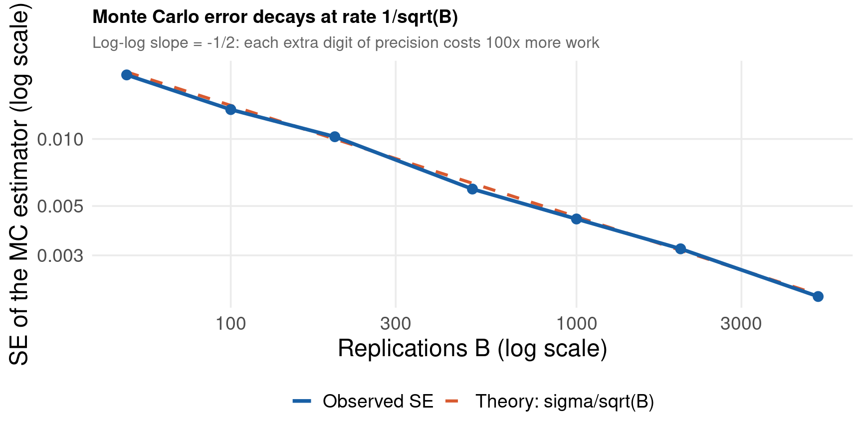
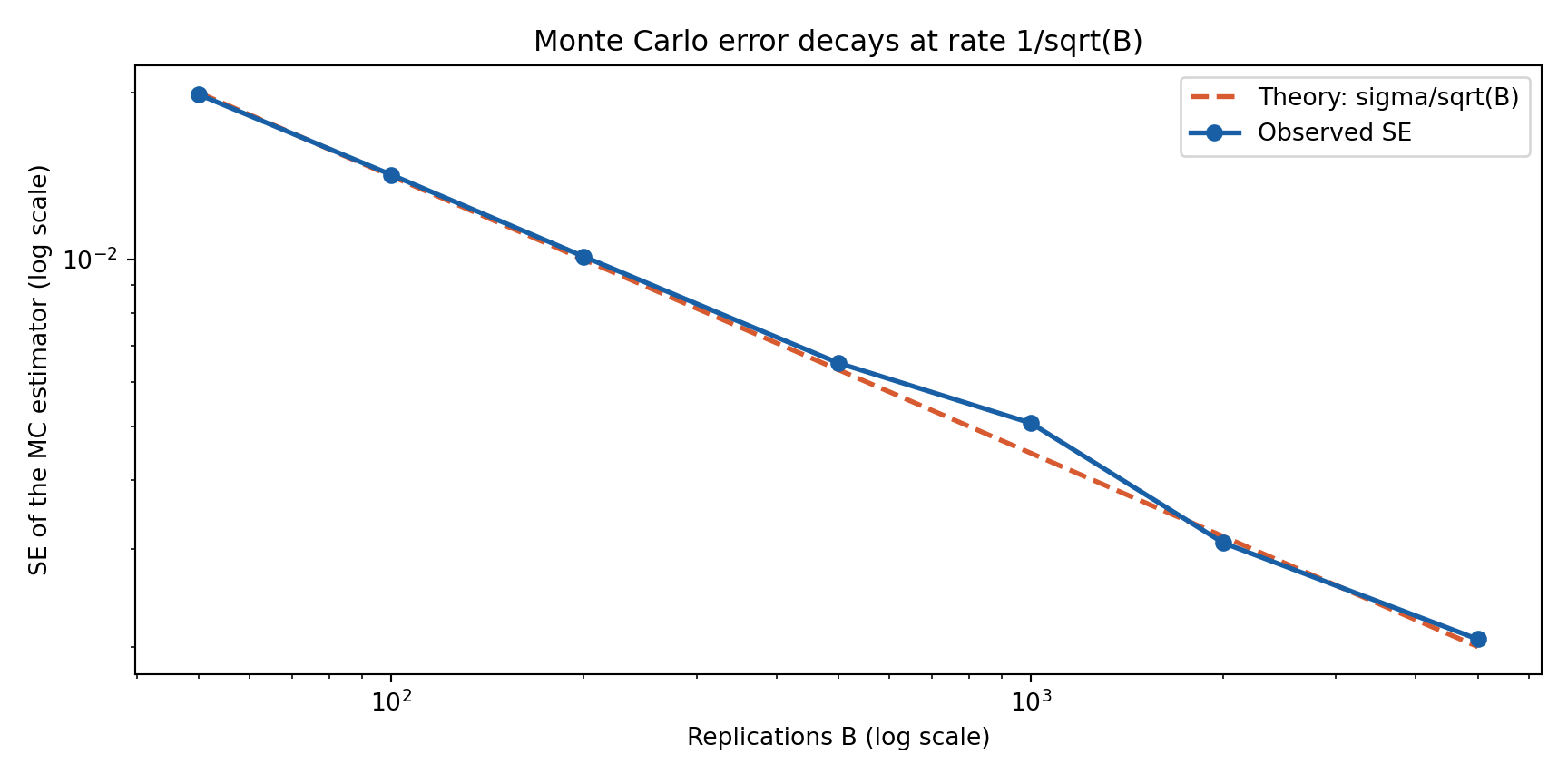
We estimate \(\theta = \mathbb{E}[\bar X_{50}]\) with \(X \sim \text{Exp}(1)\) at increasing budgets \(B\), and for each \(B\) measure the spread of \(\hat\theta_{\text{MC}}\) across 200 independent repetitions of the whole experiment:

\[ \text{SD}\!\left(\hat\theta_{\text{MC}}\right) \;\stackrel{?}{=}\; \frac{\sigma_h}{\sqrt{B}}, \qquad \sigma_h = \text{SD}(\bar X_{50}) = \frac{1}{\sqrt{50}} \]

On log-log axes the observed SE should fall on a straight line with slope −1/2.

set.seed(14159)
B_seq <- c(50, 100, 200, 500, 1000, 2000, 5000)

# for each budget B: repeat the whole MC experiment 200 times, record its SD
observed_se <- numeric(length(B_seq))
for (j in seq_along(B_seq)) {
  reps <- numeric(200)
  for (r in 1:200) {
    draws <- numeric(B_seq[j])
    for (b in 1:B_seq[j]) draws[b] <- mean(rexp(50))
    reps[r] <- mean(draws)
  }
  observed_se[j] <- sd(reps)
}

df_err <- tibble(B = B_seq, observed = observed_se,
                 theory = (1 / sqrt(50)) / sqrt(B_seq))

ggplot(df_err, aes(x = B)) +
  geom_line(aes(y = theory, color = "Theory: sigma/sqrt(B)"), linewidth = 1.1, linetype = "dashed") +
  geom_line(aes(y = observed, color = "Observed SE"), linewidth = 1.3) +
  geom_point(aes(y = observed), color = "#185FA5", size = 3) +
  scale_x_log10() + scale_y_log10() +
  scale_color_manual(values = c("Observed SE" = "#185FA5", "Theory: sigma/sqrt(B)" = "#D85A30"), name = NULL) +
  labs(x = "Replications B (log scale)", y = "SE of the MC estimator (log scale)",
       title = "Monte Carlo error decays at rate 1/sqrt(B)",
       subtitle = "Log-log slope = -1/2: each extra digit of precision costs 100x more work") +
  theme_lecture

import numpy as np
import matplotlib.pyplot as plt

rng = np.random.default_rng(14159)
B_seq = [50, 100, 200, 500, 1000, 2000, 5000]

observed_se = []
for B in B_seq:
    reps = np.empty(200)
    for r in range(200):
        draws = rng.exponential(size=(B, 50)).mean(axis=1)
        reps[r] = draws.mean()
    observed_se.append(reps.std(ddof=1))

theory = (1 / np.sqrt(50)) / np.sqrt(B_seq)

fig, ax = plt.subplots(figsize=(9, 4.5))
ax.loglog(B_seq, theory, "--", color="#D85A30", lw=2, label="Theory: sigma/sqrt(B)")
ax.loglog(B_seq, observed_se, "-o", color="#185FA5", lw=2, ms=6, label="Observed SE")
ax.set_xlabel("Replications B (log scale)")
ax.set_ylabel("SE of the MC estimator (log scale)")
ax.set_title("Monte Carlo error decays at rate 1/sqrt(B)")
ax.legend()
plt.tight_layout(); plt.show()

* SD of the MC estimator across 200 repeats of the whole experiment.
* Shortcut: the mean of 50 iid Exp(1) draws is exactly Gamma(50, 1/50).
set seed 14159
tempfile results
tempname h
postfile `h' B se using `results'
foreach B of numlist 50 100 200 500 1000 2000 5000 {
  quietly {
    clear
    set obs `=200*`B''
    gen m = rgamma(50, 1/50)
    gen rep = ceil(_n / `B')
    collapse (mean) est = m, by(rep)
    summarize est
  }
  post `h' (`B') (r(sd))
}
postclose `h'
use `results', clear
gen theory = (1/sqrt(50)) / sqrt(B)
format se theory %8.5f
list B se theory, noobs
twoway (line theory B, lcolor(red) lpattern(dash) lwidth(medthick)) ///
       (connected se B, lcolor(navy) mcolor(navy) msize(medium)), ///
  xscale(log) yscale(log) ///
  legend(order(2 "Observed SE" 1 "Theory: sigma/sqrt(B)")) ///
  xtitle("Replications B (log scale)") ytitle("SE of the MC estimator (log scale)") ///
  title("Monte Carlo error decays at rate 1/sqrt(B)")

  |    B        se    theory |
  |--------------------------|
  |   50   0.01801   0.02000 |
  |  100   0.01341   0.01414 |
  |  200   0.01030   0.01000 |
  |  500   0.00561   0.00632 |
  | 1000   0.00460   0.00447 |
  |--------------------------|
  | 2000   0.00319   0.00316 |
  | 5000   0.00190   0.00200 |
  +--------------------------+

Part II: The CLT Laboratory

Verifying — and breaking — the Central Limit Theorem by simulation

The Central Limit Theorem

• The Theorem
• The Conditions
• Why Exp(1)?

Theorem (Lévy–Lindeberg). Let \(X_1, \ldots, X_n \overset{\text{iid}}{\sim} F\) with \(\mathbb{E}[X] = \mu < \infty\) and \(\text{Var}(X) = \sigma^2 < \infty\). Then:

\[ Z_n \equiv \frac{\sqrt{n}\,(\bar{X}_n - \mu)}{\sigma} \xrightarrow{\;d\;} \mathcal{N}(0, 1) \quad \text{as } n \to \infty \]

The distribution \(F\) is irrelevant in the limit — Exponential, Bernoulli, \(t(3)\), all give the same \(\mathcal{N}(0,1)\) standardised sample mean. That is the miracle, and it is why so much of econometrics “works”.

All three must hold — and each fails for data economists actually use:

Condition	Meaning	Fails for…
iid	independent, identical draws	time series, clustered data
\(\mu < \infty\)	finite mean	Cauchy, Pareto \((\alpha \le 1)\)
\(\sigma^2 < \infty\)	finite variance	\(t_\nu\) for \(\nu \le 2\), Cauchy

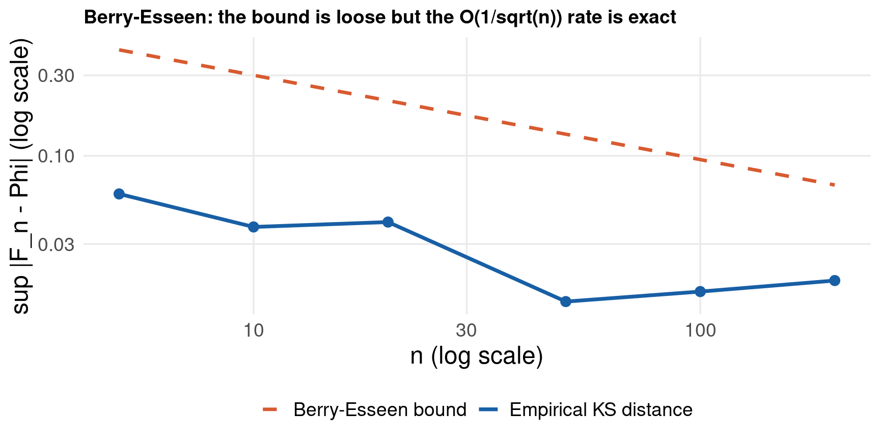
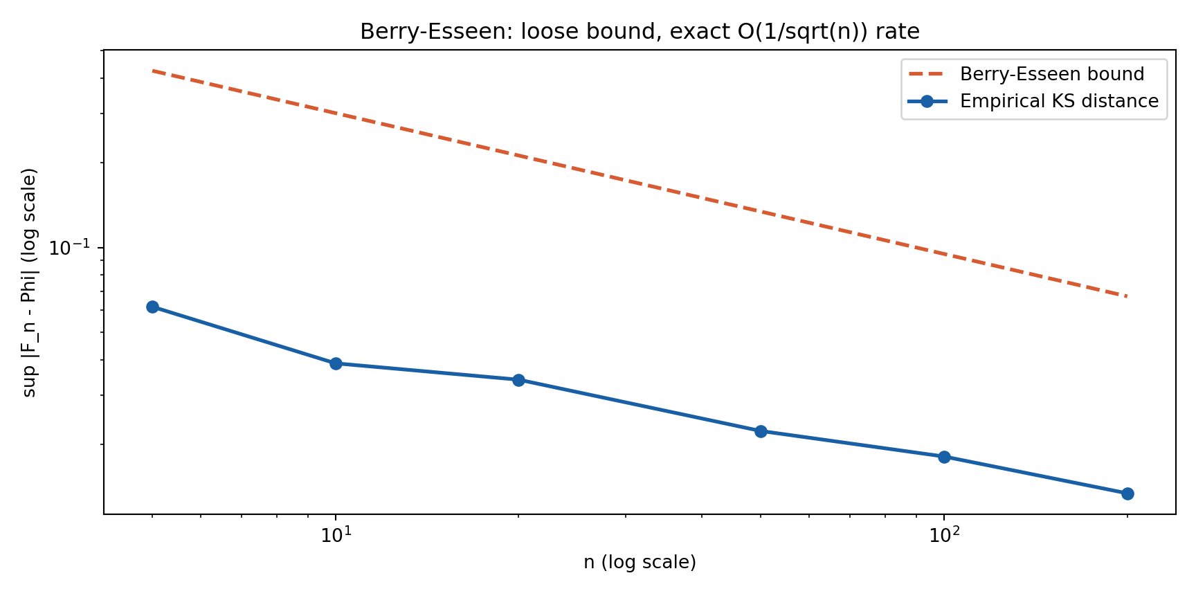
The convergence rate is bounded by the Berry–Esseen theorem:

\[ \sup_x \left| F_{Z_n}(x) - \Phi(x) \right| \leq \frac{C \cdot \rho}{\sigma^3 \sqrt{n}}, \qquad \rho = \mathbb{E}\!\left[|X - \mu|^3\right], \quad C \approx 0.4748 \]

More skewness (larger \(\rho\)) → slower convergence → worse finite-sample inference.

We stress-test the CLT with a strongly skewed parent distribution:

\[ X \sim \text{Exp}(1): \qquad \mu = 1, \qquad \sigma^2 = 1, \qquad \text{skewness } \gamma_1 = 2, \qquad \text{support } (0, \infty) \]

• Clearly non-Normal — support is one-sided, density peaks at zero
• Known mean and variance, so we can standardise exactly
• The skew makes convergence visually dramatic: at \(n=5\) the histogram is lopsided, by \(n=100\) it hugs the Gaussian curve

DGP — Standardised Sample Means

• Specification

For each sample size \(n \in \{5, 10, 30, 100\}\) and each replication \(b = 1, \dots, 5000\):

\[ X_{1b}, \ldots, X_{nb} \overset{\text{iid}}{\sim} \text{Exp}(1), \qquad Z_{nb} = \sqrt{n}\,\big(\bar{X}_{nb} - 1\big) \]

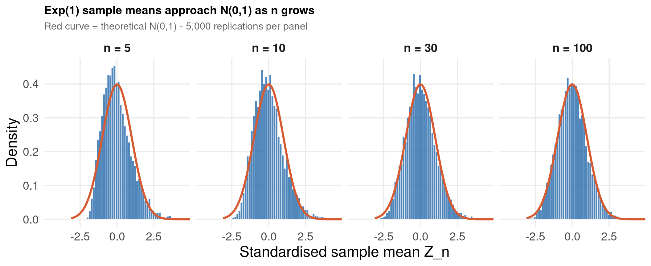
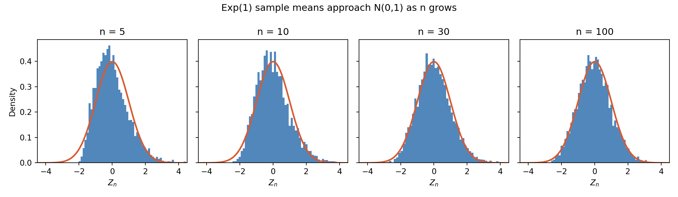
R generates all \(4 \times 5000\) standardised means and writes them to ../data/monte-carlo-clt.csv; Python and Stata read the same file, so the three languages plot literally the same simulated draws.

set.seed(14159)
n_vals <- c(5, 10, 30, 100)
B <- 5000

rows <- list()
for (nv in n_vals) {
  z <- numeric(B)
  for (b in 1:B) z[b] <- sqrt(nv) * (mean(rexp(nv)) - 1)
  rows[[length(rows) + 1]] <- tibble(n = nv, b = 1:B, z = z)
}
clt_df <- bind_rows(rows)
write.csv(clt_df, "../data/monte-carlo-clt.csv", row.names = FALSE)

Wrote ../data/monte-carlo-clt.csv : 20000 rows

# A tibble: 4 × 4
      n   mean_z  sd_z  skew
  <dbl>    <dbl> <dbl> <dbl>
1     5  0.00546 0.986 0.829
2    10  0.00752 1.01  0.665
3    30  0.0216  1.02  0.393
4   100 -0.0222  0.993 0.193

import pandas as pd

clt = pd.read_csv("../data/monte-carlo-clt.csv")   # always reads R's CSV
print(clt.groupby("n")["z"].agg(["mean", "std", "skew"]).round(3))

      mean    std   skew
n                       
5    0.005  0.986  0.829
10   0.008  1.011  0.666
30   0.022  1.017  0.393
100 -0.022  0.993  0.193

import delimited "../data/monte-carlo-clt.csv", clear
quietly destring _all, replace
tabstat z, by(n) statistics(mean sd skewness) format(%9.3f)

(encoding automatically selected: ISO-8859-9)
(3 vars, 20,000 obs)



Summary for variables: z
Group variable: n 

       n |      Mean        SD  Skewness
---------+------------------------------
       5 |     0.005     0.986     0.829
      10 |     0.008     1.011     0.666
      30 |     0.022     1.017     0.393
     100 |    -0.022     0.993     0.193
---------+------------------------------
   Total |     0.003     1.002     0.519
----------------------------------------

CLT Convergence — Histograms

clt_df <- read.csv("../data/monte-carlo-clt.csv")
clt_df$n_lab <- factor(paste0("n = ", clt_df$n), levels = paste0("n = ", c(5, 10, 30, 100)))

ggplot(clt_df, aes(x = z)) +
  geom_histogram(aes(y = after_stat(density)), bins = 60,
                 fill = "#185FA5", alpha = 0.75, color = "white", linewidth = 0.15) +
  stat_function(fun = dnorm, color = "#D85A30", linewidth = 1.2) +
  facet_wrap(~n_lab, nrow = 1) +
  coord_cartesian(xlim = c(-4.5, 4.5)) +
  labs(x = "Standardised sample mean Z_n", y = "Density",
       title = "Exp(1) sample means approach N(0,1) as n grows",
       subtitle = "Red curve = theoretical N(0,1) - 5,000 replications per panel") +
  theme_lecture

import pandas as pd
import numpy as np
import matplotlib.pyplot as plt
from scipy import stats

clt = pd.read_csv("../data/monte-carlo-clt.csv")
xs = np.linspace(-4.5, 4.5, 300)

fig, axes = plt.subplots(1, 4, figsize=(12, 3.5), sharey=True)
for ax, nv in zip(axes, [5, 10, 30, 100]):
    z = clt.loc[clt["n"] == nv, "z"]
    ax.hist(z, bins=60, density=True, color="#185FA5", alpha=0.75)
    ax.plot(xs, stats.norm.pdf(xs), color="#D85A30", lw=2)
    ax.set_xlim(-4.5, 4.5)
    ax.set_title(f"n = {nv}")
    ax.set_xlabel(r"$Z_n$")
axes[0].set_ylabel("Density")
fig.suptitle("Exp(1) sample means approach N(0,1) as n grows")
plt.tight_layout(); plt.show()

import delimited "../data/monte-carlo-clt.csv", clear
quietly destring _all, replace
twoway (histogram z if n == 5,   density bin(60) color(navy%60)) ///
       (histogram z if n == 100, density bin(60) color(red%50))  ///
       (function y = normalden(x), range(-4.5 4.5) lcolor(black) lwidth(medthick)), ///
  legend(label(1 "n = 5") label(2 "n = 100") label(3 "N(0,1)")) ///
  title("CLT convergence: n = 5 vs n = 100") xtitle("Z_n")

(encoding automatically selected: ISO-8859-9)
(3 vars, 20,000 obs)

CLT Convergence — QQ Plots and Normality Tests

clt_df <- read.csv("../data/monte-carlo-clt.csv")
z5   <- clt_df$z[clt_df$n == 5]
z100 <- clt_df$z[clt_df$n == 100]

par(mfrow = c(1, 2))
qqnorm(z5,   main = "n = 5: skew visible in the tails", col = adjustcolor("#185FA5", 0.3), pch = 16, cex = 0.5)
qqline(z5,   col = "#D85A30", lwd = 2.5)
qqnorm(z100, main = "n = 100: nearly perfect Normal",   col = adjustcolor("#1D9E75", 0.3), pch = 16, cex = 0.5)
qqline(z100, col = "#D85A30", lwd = 2.5)

ks5   <- ks.test(z5,   "pnorm")
ks100 <- ks.test(z100, "pnorm")
cat(sprintf("KS test n=5  : D = %.4f, p = %.4g\n", ks5$statistic, ks5$p.value))
cat(sprintf("KS test n=100: D = %.4f, p = %.4g\n", ks100$statistic, ks100$p.value))

KS test n=5  : D = 0.0571, p = 1.398e-14

KS test n=100: D = 0.0243, p = 0.005526

import pandas as pd
import matplotlib.pyplot as plt
from scipy import stats

clt = pd.read_csv("../data/monte-carlo-clt.csv")
z5   = clt.loc[clt["n"] == 5,   "z"]
z100 = clt.loc[clt["n"] == 100, "z"]

fig, axes = plt.subplots(1, 2, figsize=(9, 4.2))
stats.probplot(z5,   dist="norm", plot=axes[0])

((array([-3.63568806, -3.40036853, -3.27067228, ...,  3.27067228,
        3.40036853,  3.63568806], shape=(5000,)), array([-2.0217059 , -1.94982325, -1.92504824, ...,  4.61648051,
        4.65449577,  5.13381114], shape=(5000,))), (np.float64(0.9679261943595228), np.float64(0.005460012731728331), np.float64(0.9810236686803661)))

stats.probplot(z100, dist="norm", plot=axes[1])

((array([-3.63568806, -3.40036853, -3.27067228, ...,  3.27067228,
        3.40036853,  3.63568806], shape=(5000,)), array([-3.08989905, -2.92504251, -2.92300286, ...,  3.26012805,
        3.69148337,  3.82515237], shape=(5000,))), (np.float64(0.9924984891357138), np.float64(-0.022236037026115946), np.float64(0.9988104424213411)))

axes[0].set_title("n = 5: skew visible in the tails")
axes[1].set_title("n = 100: nearly perfect Normal")
for ax in axes:
    ax.get_lines()[0].set(color="#185FA5", markersize=2, alpha=0.4)
    ax.get_lines()[1].set(color="#D85A30", linewidth=2)

[None, None, None]
[None, None]
[None, None, None]
[None, None]

plt.tight_layout(); plt.show()

for nv, z in [(5, z5), (100, z100)]:
    D, p = stats.kstest(z, "norm")
    print(f"KS test n={nv:<3}: D = {D:.4f}, p = {p:.4g}")

KS test n=5  : D = 0.0571, p = 1.316e-14
KS test n=100: D = 0.0243, p = 0.005434

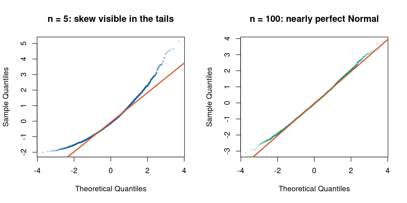
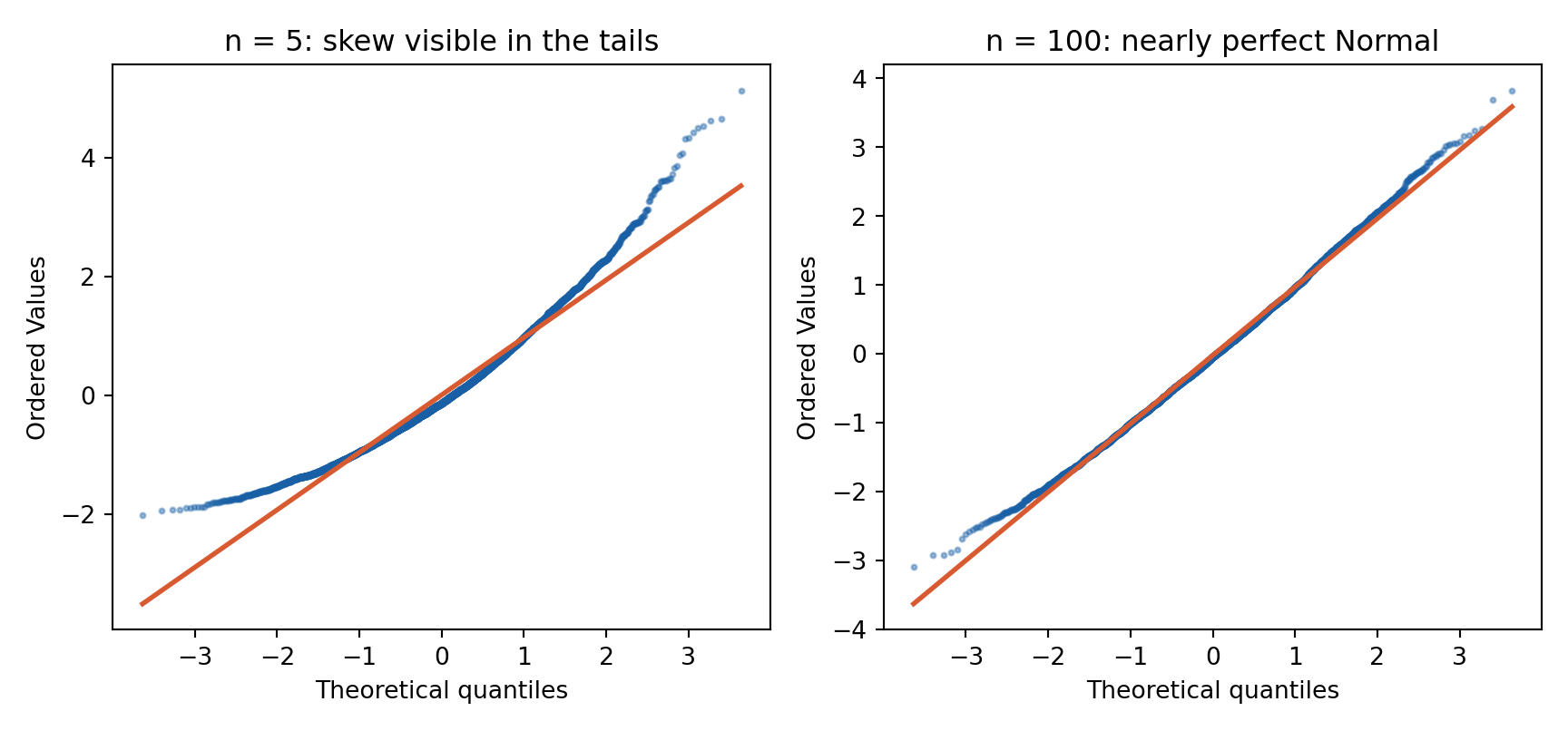
import delimited "../data/monte-carlo-clt.csv", clear
quietly destring _all, replace
qnorm z if n == 5, mcolor(navy%40) msize(tiny) rlopts(lcolor(red)) ///
  title("QQ plot of Z_n, n = 5")
display "Skewness/kurtosis normality test, n = 5:"
sktest z if n == 5
display "Skewness/kurtosis normality test, n = 100:"
sktest z if n == 100

(encoding automatically selected: ISO-8859-9)
(3 vars, 20,000 obs)




Skewness/kurtosis normality test, n = 5:


Skewness and kurtosis tests for normality
                                                         ----- Joint test -----
    Variable |       Obs   Pr(skewness)   Pr(kurtosis)   Adj chi2(2)  Prob>chi2
-------------+-----------------------------------------------------------------
           z |     5,000         0.0000         0.0000        440.80     0.0000

Skewness/kurtosis normality test, n = 100:


Skewness and kurtosis tests for normality
                                                         ----- Joint test -----
    Variable |       Obs   Pr(skewness)   Pr(kurtosis)   Adj chi2(2)  Prob>chi2
-------------+-----------------------------------------------------------------
           z |     5,000         0.0000         0.8258         27.99     0.0000

When the CLT Fails — the Cauchy Distribution

• Why It Fails

The Cauchy distribution is symmetric but has no finite mean (\(\mathbb{E}[|X|] = \infty\)), so both CLT moment conditions fail. By its characteristic function:

\[ \bar{X}_n \sim \text{Cauchy}(0, 1) \quad \text{for every } n \]

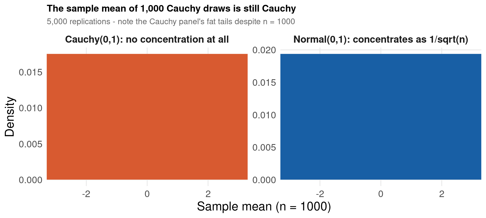
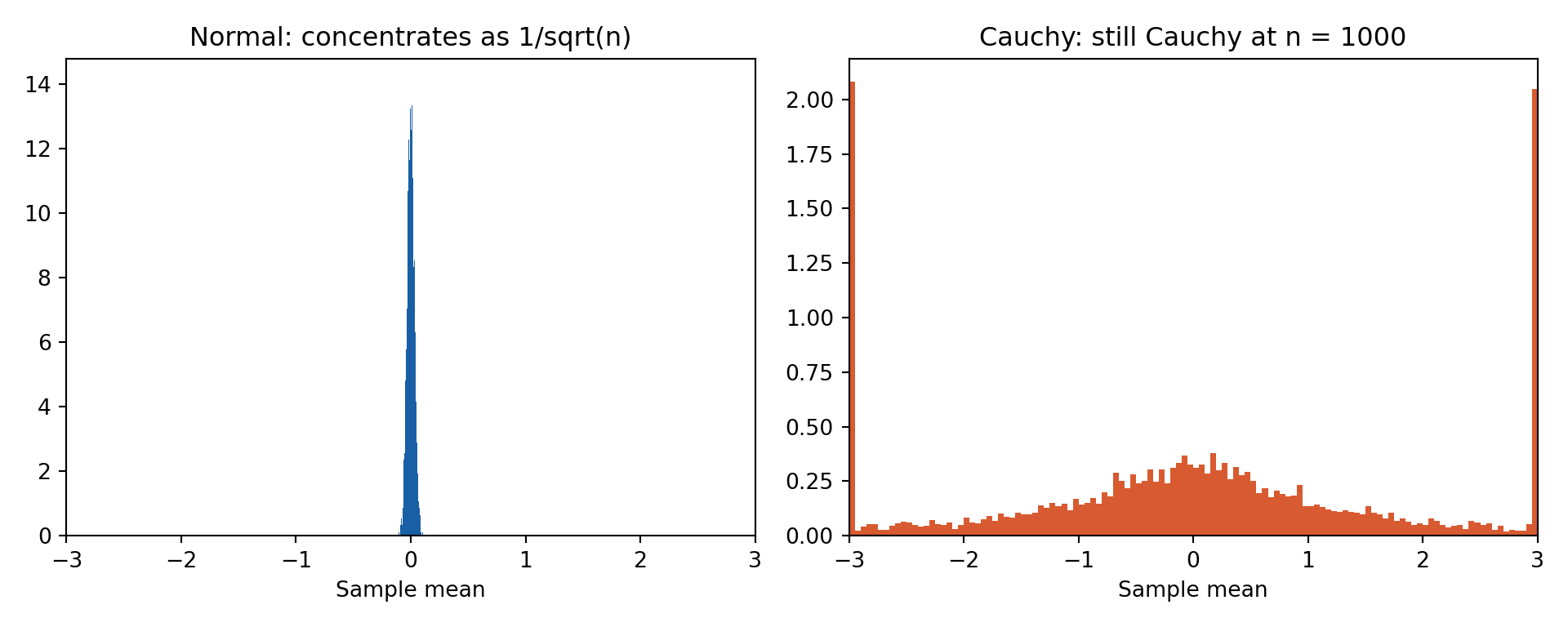
The sample mean of \(n\) Cauchy draws is again Cauchy — averaging produces zero concentration, no matter how large \(n\) gets. Any MC study that quietly assumes a finite variance (heavy-tailed returns! Pareto firm sizes!) can fall into this trap.

set.seed(14159)
B <- 5000; n <- 1000

means_normal <- numeric(B)
means_cauchy <- numeric(B)
for (b in 1:B) {
  means_normal[b] <- mean(rnorm(n))
  means_cauchy[b] <- mean(rcauchy(n))
}

df_c <- bind_rows(
  tibble(mean = means_normal, dist = "Normal(0,1): concentrates as 1/sqrt(n)"),
  tibble(mean = means_cauchy, dist = "Cauchy(0,1): no concentration at all")
)

ggplot(df_c, aes(x = mean, fill = dist)) +
  geom_histogram(aes(y = after_stat(density)), bins = 120, color = "white", linewidth = 0.1) +
  facet_wrap(~dist, scales = "free_y") +
  coord_cartesian(xlim = c(-3, 3)) +
  scale_fill_manual(values = c("#D85A30", "#185FA5"), guide = "none") +
  labs(x = "Sample mean (n = 1000)", y = "Density",
       title = "The sample mean of 1,000 Cauchy draws is still Cauchy",
       subtitle = "5,000 replications - note the Cauchy panel's fat tails despite n = 1000") +
  theme_lecture

import numpy as np
import matplotlib.pyplot as plt

rng = np.random.default_rng(14159)
B, n = 5000, 1000
means_normal = rng.standard_normal((B, n)).mean(axis=1)
means_cauchy = rng.standard_cauchy((B, n)).mean(axis=1)

fig, axes = plt.subplots(1, 2, figsize=(10, 4))
axes[0].hist(means_normal, bins=120, density=True, color="#185FA5")
axes[0].set_title("Normal: concentrates as 1/sqrt(n)")
axes[1].hist(np.clip(means_cauchy, -3, 3), bins=120, density=True, color="#D85A30")
axes[1].set_title("Cauchy: still Cauchy at n = 1000")
for ax in axes:
    ax.set_xlim(-3, 3); ax.set_xlabel("Sample mean")
plt.tight_layout(); plt.show()

print(f"SD across replications  Normal: {means_normal.std(ddof=1):.4f}   (theory 1/sqrt(1000) = {1/np.sqrt(1000):.4f})")

SD across replications  Normal: 0.0314   (theory 1/sqrt(1000) = 0.0316)

print(f"IQR across replications Cauchy: {np.subtract(*np.percentile(means_cauchy, [75, 25])):.4f}   (Cauchy IQR = 2, any n)")

IQR across replications Cauchy: 1.9859   (Cauchy IQR = 2, any n)

* 5000 replications of the mean of n = 1000 draws, Normal vs Cauchy.
* A Cauchy draw is the ratio of two independent standard Normals.
quietly {
  clear
  set seed 14159
  set obs 5000000
  gen g   = ceil(_n / 1000)
  gen zn  = rnormal()
  gen zc  = rnormal() / rnormal()
  collapse (mean) m_normal = zn m_cauchy = zc, by(g)
}
display "Across 5000 replications of the mean (n = 1000 each):"
summarize m_normal m_cauchy, detail
display "Normal SD ~ " %6.4f 1/sqrt(1000) " as theory predicts; Cauchy quartiles stay O(1)."
twoway (histogram m_cauchy if abs(m_cauchy) < 3, density bin(120) color(red%50)) ///
       (histogram m_normal, density bin(60) color(navy%60)), ///
  legend(label(2 "Normal: concentrates as 1/sqrt(n)") label(1 "Cauchy: still Cauchy")) ///
  xtitle("Sample mean (n = 1000)") ///
  title("The sample mean of 1000 Cauchy draws is still Cauchy")

Across 5000 replications of the mean (n = 1000 each):

                          (mean) zn
-------------------------------------------------------------
      Percentiles      Smallest
 1%    -.0742439      -.1140527
 5%    -.0538611      -.1116729
10%    -.0420627      -.1022158       Obs               5,000
25%    -.0217698      -.1002853       Sum of wgt.       5,000

50%     .0000873                      Mean          -.0003209
                        Largest       Std. dev.      .0320061
75%     .0213199        .098508
90%     .0407568       .1038475       Variance       .0010244
95%      .052478       .1072775       Skewness      -.0346208
99%     .0736517       .1261754       Kurtosis       2.924206

                          (mean) zc
-------------------------------------------------------------
      Percentiles      Smallest
 1%    -28.89108      -979.2396
 5%    -6.542495      -720.3051
10%    -3.096384      -370.7444       Obs               5,000
25%    -.9885845      -328.3892       Sum of wgt.       5,000

50%      .012767                      Mean           .0154416
                        Largest       Std. dev.       28.0314
75%      1.00101        253.863
90%     3.171221       341.6121       Variance       785.7593
95%     6.879598         365.36       Skewness      -.0021905
99%     31.77426       1093.115       Kurtosis       873.2744

Normal SD ~ 0.0316 as theory predicts; Cauchy quartiles stay O(1).

The Berry–Esseen Bound, Verified

• Setup

For \(\text{Exp}(1)\): \(\sigma = 1\) and \(\rho = \mathbb{E}[|X-1|^3] = 2\), so

\[ \sup_x \left| F_{Z_n}(x) - \Phi(x) \right| \;\le\; \frac{0.4748 \times 2}{\sqrt{n}} \]

We measure the left side by the Kolmogorov–Smirnov statistic of simulated \(Z_n\) against \(\Phi\), for \(n \in \{5, 10, 20, 50, 100, 200\}\). The bound is conservative, but the slope on log-log axes must be −1/2.

set.seed(14159)
n_be <- c(5, 10, 20, 50, 100, 200)
B <- 20000

emp <- numeric(length(n_be))
for (j in seq_along(n_be)) {
  z <- sqrt(n_be[j]) * (colMeans(matrix(rexp(n_be[j] * B), nrow = n_be[j])) - 1)
  emp[j] <- unname(ks.test(z, "pnorm")$statistic)
}
df_be <- tibble(n = n_be, empirical = emp, bound = 0.4748 * 2 / sqrt(n_be))

ggplot(df_be, aes(x = n)) +
  geom_line(aes(y = bound, color = "Berry-Esseen bound"), linewidth = 1.2, linetype = "dashed") +
  geom_line(aes(y = empirical, color = "Empirical KS distance"), linewidth = 1.3) +
  geom_point(aes(y = empirical), color = "#185FA5", size = 3) +
  scale_x_log10() + scale_y_log10() +
  scale_color_manual(values = c("Empirical KS distance" = "#185FA5", "Berry-Esseen bound" = "#D85A30"), name = NULL) +
  labs(x = "n (log scale)", y = "sup |F_n - Phi| (log scale)",
       title = "Berry-Esseen: the bound is loose but the O(1/sqrt(n)) rate is exact") +
  theme_lecture

import numpy as np
import matplotlib.pyplot as plt
from scipy import stats

rng = np.random.default_rng(14159)
n_be = [5, 10, 20, 50, 100, 200]
B = 20000

emp = []
for nv in n_be:
    z = np.sqrt(nv) * (rng.exponential(size=(B, nv)).mean(axis=1) - 1)
    emp.append(stats.kstest(z, "norm").statistic)
bound = 0.4748 * 2 / np.sqrt(n_be)

fig, ax = plt.subplots(figsize=(9, 4.5))
ax.loglog(n_be, bound, "--", color="#D85A30", lw=2, label="Berry-Esseen bound")
ax.loglog(n_be, emp, "-o", color="#185FA5", lw=2, ms=6, label="Empirical KS distance")
ax.set_xlabel("n (log scale)"); ax.set_ylabel("sup |F_n - Phi| (log scale)")
ax.set_title("Berry-Esseen: loose bound, exact O(1/sqrt(n)) rate")
ax.legend(); plt.tight_layout(); plt.show()

Part III: Estimators under the Microscope

OLS bias, RMSE and t-test size in finite samples

The Gauss–Markov Benchmark

• The Assumptions
• The Experiment

\[ \mathbf{y} = \mathbf{X}\boldsymbol{\beta} + \boldsymbol{\varepsilon}, \qquad \hat{\boldsymbol{\beta}} = (\mathbf{X}'\mathbf{X})^{-1}\mathbf{X}'\mathbf{y} = \boldsymbol{\beta} + (\mathbf{X}'\mathbf{X})^{-1}\mathbf{X}'\boldsymbol{\varepsilon} \]

#	Assumption	Consequence if violated
A1	Linearity	wrong functional form
A2	Full rank of \(\mathbf{X}\)	multicollinearity
A3	Strict exogeneity: \(\mathbb{E}[\boldsymbol{\varepsilon}|\mathbf{X}] = \mathbf{0}\)	biased OLS
A4	Spherical errors: \(\mathbb{E}[\boldsymbol{\varepsilon}\boldsymbol{\varepsilon}'|\mathbf{X}] = \sigma^2\mathbf{I}\)	wrong standard errors
A5	Normality of \(\boldsymbol{\varepsilon}\)	no exact finite-sample \(t\) inference

Unbiasedness needs only A3:

\[ \mathbb{E}[\hat{\boldsymbol{\beta}} \mid \mathbf{X}] = \boldsymbol{\beta} + (\mathbf{X}'\mathbf{X})^{-1}\mathbf{X}'\,\underbrace{\mathbb{E}[\boldsymbol{\varepsilon}\mid\mathbf{X}]}_{=\,\mathbf{0}} = \boldsymbol{\beta} \]

We hold A1–A4 and break A5 — three error distributions, four sample sizes:

\[ \varepsilon \sim \mathcal{N}(0,1), \qquad \varepsilon \sim t(3), \qquad \varepsilon \sim \chi^2(2) - 2, \qquad n \in \{30, 50, 100, 300\} \]

with true \(\boldsymbol{\beta} = (1,\ 2,\ -0.5)'\). Three metrics per cell, all for the slope \(\beta_1\):

\[ \widehat{\text{Bias}} = \frac{1}{B}\sum_b \hat\beta_1^{(b)} - \beta_1, \qquad \widehat{\text{RMSE}} = \sqrt{\widehat{\text{Bias}}^2 + \widehat{\text{Var}}}, \qquad \hat\pi_{0.05} = \frac{1}{B}\sum_b \mathbf{1}\!\left[p^{(b)} < 0.05\right] \text{ under } H_0 \]

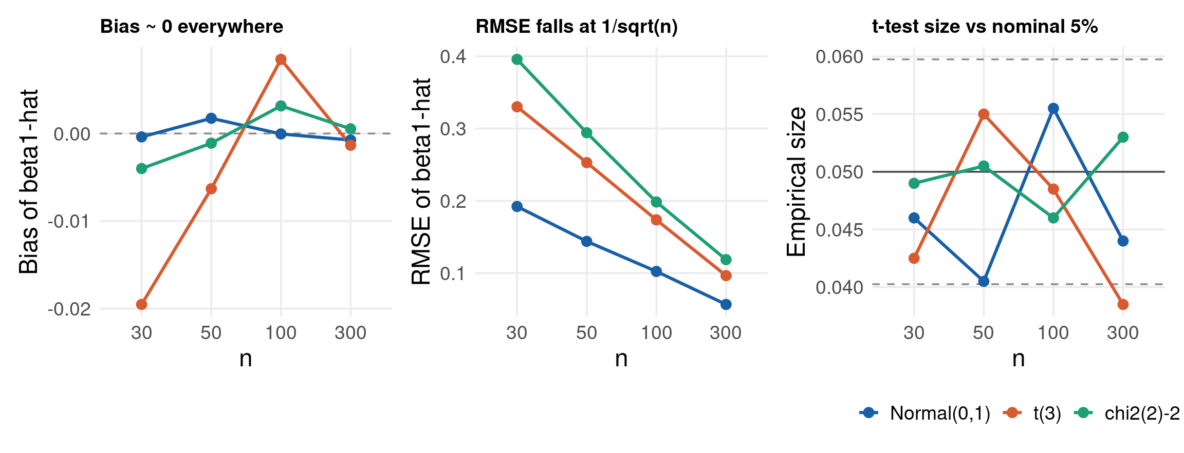
• Prediction from theory: bias ≈ 0 everywhere (A3 holds); RMSE larger for heavy tails; \(t\)-test size distorted at small \(n\) with skewed errors, correct as \(n\) grows
• What Gauss–Markov does not say: anything about finite-sample size when A5 fails — that is exactly the gap MC fills

DGP — One Shared Dataset, Three Engines

• Specification

Before the full MC loop, one single simulated dataset (\(n = 200\), skewed errors) that all three languages estimate, to confirm the engines agree to machine precision:

\[ y_i = 1 + 2\,x_{1i} - 0.5\,x_{2i} + \varepsilon_i, \qquad x_{1i}, x_{2i} \sim \mathcal{N}(0,1), \qquad \varepsilon_i \sim \chi^2(2) - 2 \]

R generates and writes ../data/monte-carlo-ols.csv; Python and Stata read it.

set.seed(14159)
n <- 200
x1 <- rnorm(n)
x2 <- rnorm(n)
e  <- rchisq(n, df = 2) - 2
y  <- 1 + 2 * x1 - 0.5 * x2 + e
ols_df <- data.frame(y = y, x1 = x1, x2 = x2)
write.csv(ols_df, "../data/monte-carlo-ols.csv", row.names = FALSE)

fit <- lm(y ~ x1 + x2, data = ols_df)
summary(fit)$coefficients

Wrote ../data/monte-carlo-ols.csv : 200 rows

            Estimate Std. Error t value Pr(>|t|)
(Intercept)   1.1139     0.1672  6.6633   0.0000
x1            1.8168     0.1635 11.1125   0.0000
x2           -0.3193     0.1610 -1.9839   0.0487

import pandas as pd
import statsmodels.api as sm

df = pd.read_csv("../data/monte-carlo-ols.csv")   # always reads R's CSV
X = sm.add_constant(df[["x1", "x2"]])
res = sm.OLS(df["y"], X).fit()
print(res.summary().tables[1])

==============================================================================
                 coef    std err          t      P>|t|      [0.025      0.975]
------------------------------------------------------------------------------
const          1.1139      0.167      6.663      0.000       0.784       1.444
x1             1.8168      0.163     11.113      0.000       1.494       2.139
x2            -0.3193      0.161     -1.984      0.049      -0.637      -0.002
==============================================================================

import delimited "../data/monte-carlo-ols.csv", clear
quietly destring _all, replace
regress y x1 x2

(encoding automatically selected: ISO-8859-1)
(3 vars, 200 obs)

      Source |       SS           df       MS      Number of obs   =       200
-------------+----------------------------------   F(2, 197)       =     63.89
       Model |      692.87         2     346.435   Prob > F        =    0.0000
    Residual |  1068.28973       197   5.4227905   R-squared       =    0.3934
-------------+----------------------------------   Adj R-squared   =    0.3873
       Total |  1761.15973       199  8.85004889   Root MSE        =    2.3287

------------------------------------------------------------------------------
           y | Coefficient  Std. err.      t    P>|t|     [95% conf. interval]
-------------+----------------------------------------------------------------
          x1 |    1.81677   .1634885    11.11   0.000     1.494358    2.139182
          x2 |  -.3193132   .1609526    -1.98   0.049    -.6367244    -.001902
       _cons |   1.113895   .1671698     6.66   0.000     .7842233    1.443567
------------------------------------------------------------------------------

The Full MC Study — Bias, RMSE and Size

• Algorithm
• Plots

1. For each error distribution \(d \in \{\text{Normal},\ t(3),\ \chi^2(2)-2\}\) and each \(n \in \{30, 50, 100, 300\}\):
2. Repeat \(B = 2000\) times: draw fresh \(\mathbf{X}\) and \(\boldsymbol{\varepsilon}\), build \(y\), fit OLS, store \(\hat\beta_1\) and the \(p\)-value of \(H_0\!: \beta_1 = 2\) (the truth — so rejections are false positives)
3. Summarise each cell: bias, RMSE, empirical size, plus the MC standard error of each
4. Plot the three metrics against \(n\), one line per error distribution
5. R runs the 12 cells in parallel with mclapply on 6 cores; Python loops the same grid; Stata runs the most distorted cell (\(\chi^2\), \(n = 30\)) with simulate

library(parallel)
beta_true <- c(1, 2, -0.5)

one_run <- function(n, dist) {
  x1 <- rnorm(n); x2 <- rnorm(n)
  e <- switch(dist,
    normal = rnorm(n),
    t3     = rt(n, df = 3),
    chi2   = rchisq(n, df = 2) - 2)
  y <- beta_true[1] + beta_true[2] * x1 + beta_true[3] * x2 + e
  cf <- summary(lm(y ~ x1 + x2))$coefficients
  # test H0: beta1 = 2 (the truth), so rejections are size
  tstat <- (cf["x1", "Estimate"] - beta_true[2]) / cf["x1", "Std. Error"]
  c(b1 = cf["x1", "Estimate"], rej = as.integer(abs(tstat) > qt(0.975, n - 3)))
}

mc_cell <- function(cell, B = 2000) {
  sims <- matrix(NA_real_, B, 2)
  for (b in 1:B) sims[b, ] <- one_run(cell$n, cell$dist)
  bias <- mean(sims[, 1]) - beta_true[2]
  data.frame(n = cell$n, dist = cell$dist,
             bias = bias, rmse = sqrt(bias^2 + var(sims[, 1])),
             size = mean(sims[, 2]),
             mcse_b1 = sd(sims[, 1]) / sqrt(B))
}

grid <- expand.grid(n = c(30, 50, 100, 300),
                    dist = c("normal", "t3", "chi2"), stringsAsFactors = FALSE)
cells <- lapply(seq_len(nrow(grid)), function(i) list(n = grid$n[i], dist = grid$dist[i]))

set.seed(14159)
res <- do.call(rbind, mclapply(cells, mc_cell, mc.set.seed = TRUE, mc.cores = 6))
print(res)

   n   dist      bias   rmse   size mcse_b1
  30   chi2 -4.00e-03 0.3958 0.0490 0.00885
  50   chi2 -1.11e-03 0.2943 0.0505 0.00658
 100   chi2  3.15e-03 0.1984 0.0460 0.00444
 300   chi2  5.39e-04 0.1187 0.0530 0.00265
  30 normal -3.86e-04 0.1922 0.0460 0.00430
  50 normal  1.74e-03 0.1439 0.0405 0.00322
 100 normal -5.01e-05 0.1023 0.0555 0.00229
 300 normal -7.46e-04 0.0567 0.0440 0.00127
  30     t3 -1.95e-02 0.3301 0.0425 0.00737
  50     t3 -6.31e-03 0.2529 0.0550 0.00565
 100     t3  8.47e-03 0.1737 0.0485 0.00388
 300     t3 -1.34e-03 0.0966 0.0385 0.00216

p_bias <- ggplot(res_ols, aes(x = factor(n), y = bias, color = dist_lab, group = dist_lab)) +
  geom_hline(yintercept = 0, linetype = "dashed", color = "grey55") +
  geom_line(linewidth = 1.1) + geom_point(size = 3) +
  scale_color_manual(values = c("#185FA5", "#D85A30", "#1D9E75"), name = NULL) +
  labs(x = "n", y = "Bias of beta1-hat", title = "Bias ~ 0 everywhere") +
  theme_lecture + theme(legend.position = "none")

p_rmse <- ggplot(res_ols, aes(x = factor(n), y = rmse, color = dist_lab, group = dist_lab)) +
  geom_line(linewidth = 1.1) + geom_point(size = 3) +
  scale_color_manual(values = c("#185FA5", "#D85A30", "#1D9E75"), name = NULL) +
  labs(x = "n", y = "RMSE of beta1-hat", title = "RMSE falls at 1/sqrt(n)") +
  theme_lecture + theme(legend.position = "none")

p_size <- ggplot(res_ols, aes(x = factor(n), y = size, color = dist_lab, group = dist_lab)) +
  geom_hline(yintercept = 0.05, linetype = "solid", color = "grey30") +
  geom_hline(yintercept = 0.05 + c(-2, 2) * sqrt(0.05 * 0.95 / 2000),
             linetype = "dashed", color = "grey55") +
  geom_line(linewidth = 1.1) + geom_point(size = 3) +
  scale_color_manual(values = c("#185FA5", "#D85A30", "#1D9E75"), name = NULL) +
  labs(x = "n", y = "Empirical size", title = "t-test size vs nominal 5%") +
  theme_lecture

p_bias + p_rmse + p_size

import numpy as np
import pandas as pd
from scipy import stats

rng = np.random.default_rng(14159)
beta = np.array([1.0, 2.0, -0.5])
B = 2000

def one_cell(n, dist):
    b1 = np.empty(B); rej = np.empty(B)
    tcrit = stats.t.ppf(0.975, n - 3)
    for b in range(B):
        X = np.column_stack([np.ones(n), rng.standard_normal(n), rng.standard_normal(n)])
        if dist == "normal":
            e = rng.standard_normal(n)
        elif dist == "t3":
            e = rng.standard_t(3, n)
        else:
            e = rng.chisquare(2, n) - 2
        y = X @ beta + e
        XtXi = np.linalg.inv(X.T @ X)
        bh = XtXi @ X.T @ y
        resid = y - X @ bh
        s2 = resid @ resid / (n - 3)
        se1 = np.sqrt(s2 * XtXi[1, 1])
        b1[b] = bh[1]
        rej[b] = abs((bh[1] - beta[1]) / se1) > tcrit
    bias = b1.mean() - beta[1]
    return bias, np.sqrt(bias**2 + b1.var(ddof=1)), rej.mean()

rows = []
for dist in ["normal", "t3", "chi2"]:
    for n in [30, 50, 100, 300]:
        bias, rmse, size = one_cell(n, dist)
        rows.append({"dist": dist, "n": n, "bias": round(bias, 4),
                     "rmse": round(rmse, 4), "size": round(size, 4)})
print(pd.DataFrame(rows).to_string(index=False))

  dist   n    bias   rmse   size
normal  30  0.0016 0.1996 0.0520
normal  50  0.0040 0.1481 0.0540
normal 100  0.0017 0.1011 0.0495
normal 300 -0.0004 0.0583 0.0520
    t3  30 -0.0038 0.3301 0.0505
    t3  50 -0.0043 0.2459 0.0465
    t3 100  0.0019 0.1739 0.0500
    t3 300  0.0016 0.1004 0.0480
  chi2  30  0.0032 0.3930 0.0465
  chi2  50 -0.0034 0.2948 0.0485
  chi2 100  0.0044 0.2019 0.0460
  chi2 300  0.0030 0.1180 0.0500

* The most distorted cell: chi2(2)-2 errors, n = 30, B = 2000
capture program drop olsmc
program define olsmc, rclass
  clear
  set obs 30
  gen x1 = rnormal()
  gen x2 = rnormal()
  gen e  = rchi2(2) - 2
  gen y  = 1 + 2*x1 - 0.5*x2 + e
  regress y x1 x2
  return scalar b1  = _b[x1]
  return scalar rej = (abs((_b[x1] - 2)/_se[x1]) > invttail(27, 0.025))
end

set seed 14159
simulate b1 = r(b1) rej = r(rej), reps(2000) nodots: olsmc
quietly summarize b1
display "Bias of b1  : " %7.4f r(mean) - 2
display "RMSE of b1  : " %7.4f sqrt((r(mean)-2)^2 + r(sd)^2)
quietly summarize rej
display "Empirical size (nominal 5%): " %6.4f r(mean)

      Command: olsmc
           b1: r(b1)
          rej: r(rej)



Bias of b1  : -0.0059

RMSE of b1  :  0.4066


Empirical size (nominal 5%): 0.0595

When A3 Fails — Endogeneity Bias Never Dies

• Setup

Now break strict exogeneity: let the regressor be correlated with the error,

\[ \begin{pmatrix} x_{1i} \\ \varepsilon_i \end{pmatrix} \sim \mathcal{N}\!\left( \mathbf{0},\ \begin{pmatrix} 1 & 0.5 \\ 0.5 & 1 \end{pmatrix} \right) \quad\Rightarrow\quad \text{plim}\; \hat\beta_1 = \beta_1 + \frac{\text{Cov}(x_1, \varepsilon)}{\text{Var}(x_1)} = 2 + 0.5 \]

• Under exogeneity, bias vanishes as \(n\) grows (consistency)
• Under endogeneity, bias converges to +0.5 — more data makes the estimate more precisely wrong
• This single MC picture is the entire motivation for instrumental variables (Part V)

set.seed(14159)
n_grid <- c(30, 100, 300, 1000, 3000)
B <- 1000

bias_endog <- numeric(length(n_grid))
bias_exog  <- numeric(length(n_grid))
for (j in seq_along(n_grid)) {
  n <- n_grid[j]
  b_en <- numeric(B); b_ex <- numeric(B)
  for (b in 1:B) {
    draws <- MASS::mvrnorm(n, mu = c(0, 0), Sigma = matrix(c(1, 0.5, 0.5, 1), 2, 2))
    x1 <- draws[, 1]; e <- draws[, 2]
    y  <- 1 + 2 * x1 + e
    b_en[b] <- coef(lm(y ~ x1))[2]
    x1c <- rnorm(n)                       # exogenous benchmark
    yc  <- 1 + 2 * x1c + rnorm(n)
    b_ex[b] <- coef(lm(yc ~ x1c))[2]
  }
  bias_endog[j] <- mean(b_en) - 2
  bias_exog[j]  <- mean(b_ex) - 2
}

df_en <- bind_rows(
  tibble(n = n_grid, bias = bias_endog, case = "Endogenous: Cov(x,e) = 0.5"),
  tibble(n = n_grid, bias = bias_exog,  case = "Exogenous benchmark")
)
ggplot(df_en, aes(x = n, y = bias, color = case)) +
  geom_hline(yintercept = c(0, 0.5), linetype = "dashed", color = "grey55") +
  geom_line(linewidth = 1.2) + geom_point(size = 3) +
  scale_x_log10() +
  scale_color_manual(values = c("#D85A30", "#1D9E75"), name = NULL) +
  labs(x = "n (log scale)", y = "Bias of beta1-hat",
       title = "Endogeneity bias does not shrink with n",
       subtitle = "It converges to Cov(x,e)/Var(x) = 0.5 - consistency is dead") +
  theme_lecture

import numpy as np

rng = np.random.default_rng(14159)
B = 1000
cov = np.array([[1.0, 0.5], [0.5, 1.0]])

print(f"{'n':>6} {'bias (endog)':>14} {'bias (exog)':>14}")

     n   bias (endog)    bias (exog)

for n in [30, 100, 300, 1000, 3000]:
    b_en = np.empty(B); b_ex = np.empty(B)
    for b in range(B):
        d = rng.multivariate_normal([0, 0], cov, size=n)
        x, e = d[:, 0], d[:, 1]
        y = 1 + 2 * x + e
        b_en[b] = np.cov(x, y)[0, 1] / x.var(ddof=1)
        xc = rng.standard_normal(n)
        yc = 1 + 2 * xc + rng.standard_normal(n)
        b_ex[b] = np.cov(xc, yc)[0, 1] / xc.var(ddof=1)
    print(f"{n:>6} {b_en.mean() - 2:>14.4f} {b_ex.mean() - 2:>14.4f}")

    30         0.4912         0.0073
   100         0.4998         0.0031
   300         0.4987         0.0002
  1000         0.5006         0.0000
  3000         0.4994         0.0000

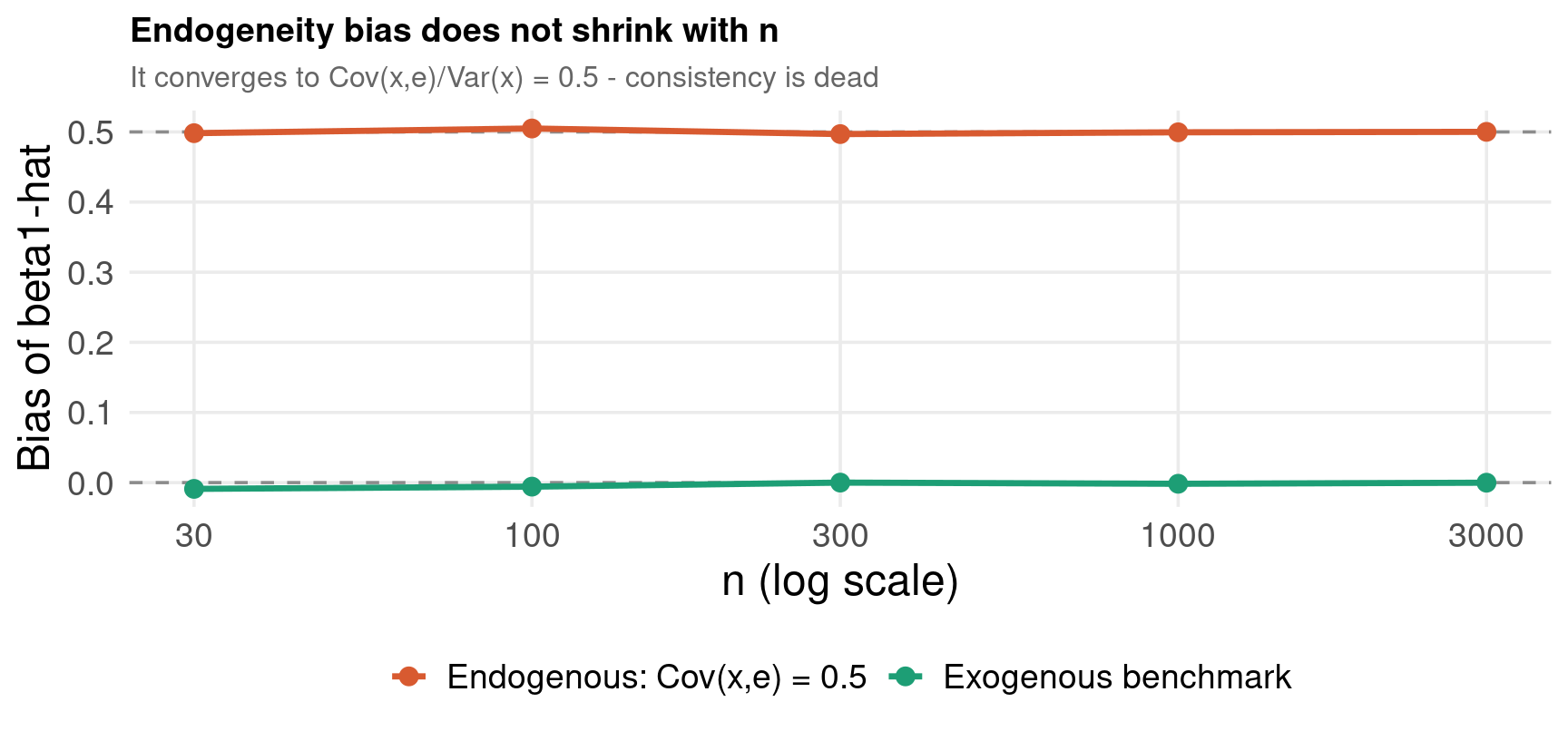
print("Endogenous bias converges to Cov(x,e)/Var(x) = 0.5")

Endogenous bias converges to Cov(x,e)/Var(x) = 0.5

capture program drop endogmc
program define endogmc, rclass
  syntax [, nobs(integer 100)]
  clear
  quietly set obs `nobs'
  gen z = rnormal()
  gen e = 0.5*z + sqrt(1 - 0.25)*rnormal()   // Corr(x,e) = 0.5
  gen x = z
  gen y = 1 + 2*x + e
  quietly regress y x
  return scalar b1 = _b[x]
end

set seed 14159
tempfile results
tempname h
postfile `h' n bias using `results'
foreach n in 30 100 300 1000 3000 {
  quietly simulate b1 = r(b1), reps(500) nodots: endogmc, nobs(`n')
  quietly summarize b1
  display "n = " %5.0f `n' "   bias of b1 = " %7.4f r(mean) - 2
  post `h' (`n') (r(mean) - 2)
}
postclose `h'
display "Bias stays at ~0.5 no matter how large n gets."
use `results', clear
twoway (connected bias n, lcolor(red) mcolor(red) msize(medium)), ///
  xscale(log) yline(0.5, lpattern(dash) lcolor(gs10)) yline(0, lpattern(dash) lcolor(gs10)) ///
  ylabel(0(0.1)0.6) xtitle("n (log scale)") ytitle("Bias of b1") ///
  title("Endogeneity bias does not shrink with n")

n =    30   bias of b1 =  0.4990
n =   100   bias of b1 =  0.4975
n =   300   bias of b1 =  0.4981
n =  1000   bias of b1 =  0.4990
n =  3000   bias of b1 =  0.5003


Bias stays at ~0.5 no matter how large n gets.

Heteroskedasticity — Classical vs Robust Standard Errors

• Setup

Keep A3 but break A4 with error variance rising in the regressor:

\[ y_i = 1 + 2 x_i + \varepsilon_i, \qquad \varepsilon_i = e^{x_i / 2}\, u_i, \qquad u_i \sim \mathcal{N}(0,1) \]

• \(\hat\beta\) is still unbiased — but the classical variance formula \(\sigma^2(\mathbf{X}'\mathbf{X})^{-1}\) is wrong
• We compare the size of the \(t\)-test on \(\beta_1\) using classical vs HC3 robust standard errors
• Prediction: classical over-rejects; HC3 restores size near 5%

set.seed(14159)
B <- 3000; n <- 100

rej_ols <- numeric(B); rej_hc3 <- numeric(B)
for (b in 1:B) {
  x <- rnorm(n)
  y <- 1 + 2 * x + exp(x / 2) * rnorm(n)
  fit <- lm(y ~ x)
  t_ols <- (coef(fit)[2] - 2) / sqrt(vcov(fit)[2, 2])
  t_hc3 <- (coef(fit)[2] - 2) / sqrt(sandwich::vcovHC(fit, type = "HC3")[2, 2])
  crit  <- qt(0.975, n - 2)
  rej_ols[b] <- abs(t_ols) > crit
  rej_hc3[b] <- abs(t_hc3) > crit
}
cat(sprintf("Classical SE size: %.4f\n", mean(rej_ols)))
cat(sprintf("HC3 robust  size : %.4f\n", mean(rej_hc3)))
cat("Nominal: 0.05  (MC SE ~ 0.004 at B = 3000)\n")

Classical SE size: 0.1613

HC3 robust  size : 0.0593

Nominal: 0.05  (MC SE ~ 0.004 at B = 3000)

import numpy as np
import statsmodels.api as sm
from scipy import stats

rng = np.random.default_rng(14159)
B, n = 3000, 100
crit = stats.t.ppf(0.975, n - 2)

rej_ols = np.empty(B); rej_hc3 = np.empty(B)
for b in range(B):
    x = rng.standard_normal(n)
    y = 1 + 2 * x + np.exp(x / 2) * rng.standard_normal(n)
    X = sm.add_constant(x)
    fit = sm.OLS(y, X).fit()
    rej_ols[b] = abs((fit.params[1] - 2) / fit.bse[1]) > crit
    fit3 = fit.get_robustcov_results(cov_type="HC3")
    rej_hc3[b] = abs((fit3.params[1] - 2) / fit3.bse[1]) > crit

print(f"Classical SE size: {rej_ols.mean():.4f}")

Classical SE size: 0.1493

print(f"HC3 robust  size : {rej_hc3.mean():.4f}")

HC3 robust  size : 0.0487

print("Nominal: 0.05")

Nominal: 0.05

capture program drop hetmc
program define hetmc, rclass
  clear
  quietly set obs 100
  gen x = rnormal()
  gen y = 1 + 2*x + exp(x/2)*rnormal()
  quietly regress y x
  return scalar rej_ols = (abs((_b[x] - 2)/_se[x]) > invttail(98, 0.025))
  quietly regress y x, vce(hc3)
  return scalar rej_hc3 = (abs((_b[x] - 2)/_se[x]) > invttail(98, 0.025))
end

set seed 14159
simulate rej_ols = r(rej_ols) rej_hc3 = r(rej_hc3), reps(2000) nodots: hetmc
quietly summarize rej_ols
display "Classical SE size: " %6.4f r(mean)
quietly summarize rej_hc3
display "HC3 robust  size : " %6.4f r(mean)
display "Nominal: 0.05"

      Command: hetmc
      rej_ols: r(rej_ols)
      rej_hc3: r(rej_hc3)



Classical SE size: 0.1440


HC3 robust  size : 0.0525

Nominal: 0.05

Part IV: Designing Tests

Simulated critical values, size and power — how new tests are born

Size and Power — the Vocabulary of Test Design

• Definitions
• The Test Designer’s Workflow
• Why the ADF Needs Simulation

For a test of \(H_0\) at nominal level \(\alpha\), the power function over the parameter \(\theta\) is

\[ \pi(\theta) = \mathbb{P}\big(\text{reject } H_0 \mid \theta\big) \]

• Size \(= \pi(\theta_0)\) — the rejection rate when \(H_0\) is true. Should equal \(\alpha\); if \(\pi(\theta_0) > \alpha\) the test over-rejects (false positives), if \(<\alpha\) it is conservative (wasted power)
• Power \(= \pi(\theta_1)\) for \(\theta_1\) under \(H_1\) — the probability of catching a real effect; should rise toward 1 as \(n\) grows or \(\theta_1\) moves away from \(\theta_0\)
• Both are estimated by the same MC device: count rejections over B replications

\[ \hat\pi = \frac{1}{B}\sum_{b=1}^{B} \mathbf{1}\!\left[\text{test rejects on dataset } b\right], \qquad \widehat{\text{SE}}(\hat\pi) = \sqrt{\frac{\hat\pi(1-\hat\pi)}{B}} \]

Every published test went through exactly this pipeline:

1. Derive the statistic and (if possible) its asymptotic distribution
2. Simulate under \(H_0\) to tabulate critical values when the distribution is non-standard — the Dickey–Fuller tables, MacKinnon response surfaces, KPSS quantiles all come from MC
3. Size study: simulate under \(H_0\) across sample sizes and nuisance DGPs (heavy tails, GARCH, serial correlation) — a test with fragile size is dead on arrival
4. Power study: simulate under a grid of alternatives, compare against competitor tests
5. Report the full size/power tables — this is the “empirical section” of every econometric theory paper

Next: we replay steps 2–4 for the most famous case, the Dickey–Fuller unit root test.

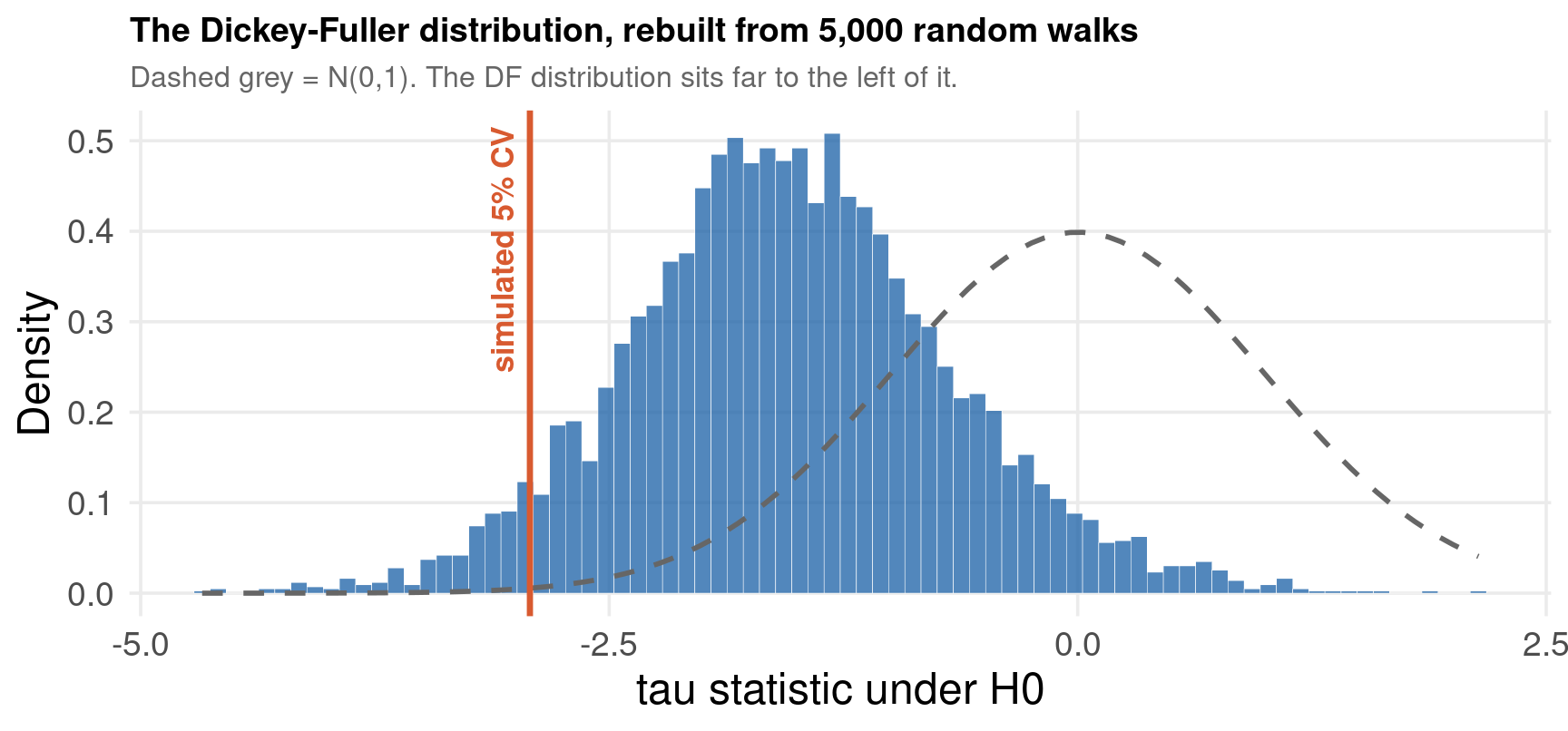
For \(y_t = \rho y_{t-1} + \varepsilon_t\), the test of \(H_0\!: \rho = 1\) uses the \(t\)-ratio \(\tau = \hat\gamma / \text{SE}(\hat\gamma)\) from \(\Delta y_t = \alpha + \gamma y_{t-1} + \varepsilon_t\). Under \(H_0\),

\[ \tau \;\xrightarrow{d}\; \frac{\int_0^1 W(r)\, dW(r)}{\left[\int_0^1 W(r)^2\, dr\right]^{1/2}} \;\;\neq\;\; t \text{ or } \mathcal{N}(0,1) \]

• The limit is a functional of Brownian motion — asymmetric, shifted left, with no closed-form CDF
• Using the \(\pm 1.96\) Normal critical values would reject a true unit root far too often
• Dickey & Fuller (1979) obtained their critical values by Monte Carlo; MacKinnon (1996) refined them with response-surface regressions on millions of simulations

Simulating Critical Values — Rebuilding the DF Table

• Algorithm

1. Impose \(H_0\): generate a pure random walk \(y_t = y_{t-1} + \varepsilon_t\), \(\varepsilon_t \sim \mathcal{N}(0,1)\), \(T = 100\)
2. Estimate the DF regression with drift, \(\Delta y_t = \alpha + \gamma y_{t-1} + \varepsilon_t\), and store \(\tau^{(b)} = \hat\gamma / \text{SE}(\hat\gamma)\)
3. Repeat \(B = 5000\) times
4. The empirical 1%, 5%, 10% quantiles of \(\{\tau^{(b)}\}\) are the critical values
5. Compare to MacKinnon’s tabulated values: \(-3.43\), \(-2.86\), \(-2.57\)

set.seed(14159)
B <- 5000; T_len <- 100

tau <- numeric(B)
for (b in 1:B) {
  y  <- cumsum(rnorm(T_len))
  dy <- diff(y)
  ylag <- y[-T_len]
  fit <- lm(dy ~ ylag)
  tau[b] <- summary(fit)$coefficients["ylag", "t value"]
}

cv <- quantile(tau, c(0.01, 0.05, 0.10))
cat("Simulated DF critical values (drift case, T = 100):\n")
print(round(cv, 3))
cat("MacKinnon tabulated:  -3.43  -2.86  -2.57\n")
cat(sprintf("Share of tau below -1.96 (naive Normal CV): %.3f - not 0.025!\n",
            mean(tau < -1.96)))

ggplot(tibble(tau = tau), aes(x = tau)) +
  geom_histogram(aes(y = after_stat(density)), bins = 80,
                 fill = "#185FA5", alpha = 0.75, color = "white", linewidth = 0.1) +
  stat_function(fun = dnorm, color = "grey40", linewidth = 1, linetype = "dashed") +
  geom_vline(xintercept = cv[2], color = "#D85A30", linewidth = 1.2) +
  annotate("text", x = cv[2] - 0.15, y = 0.38, label = "simulated 5% CV",
           color = "#D85A30", angle = 90, size = 4.5, fontface = "bold") +
  labs(x = "tau statistic under H0", y = "Density",
       title = "The Dickey-Fuller distribution, rebuilt from 5,000 random walks",
       subtitle = "Dashed grey = N(0,1). The DF distribution sits far to the left of it.") +
  theme_lecture

Simulated DF critical values (drift case, T = 100):

    1%     5%    10% 
-3.505 -2.923 -2.611 

MacKinnon tabulated:  -3.43  -2.86  -2.57

Share of tau below -1.96 (naive Normal CV): 0.306 - not 0.025!

import numpy as np

rng = np.random.default_rng(14159)
B, T = 5000, 100

tau = np.empty(B)
for b in range(B):
    y = np.cumsum(rng.standard_normal(T))
    dy = np.diff(y)
    X = np.column_stack([np.ones(T - 1), y[:-1]])
    XtXi = np.linalg.inv(X.T @ X)
    bh = XtXi @ X.T @ dy
    resid = dy - X @ bh
    s2 = resid @ resid / (T - 1 - 2)
    tau[b] = bh[1] / np.sqrt(s2 * XtXi[1, 1])

cv = np.percentile(tau, [1, 5, 10])
print("Simulated DF critical values (drift case, T = 100):")

Simulated DF critical values (drift case, T = 100):

print(np.round(cv, 3))

[-3.576 -2.969 -2.626]

print("MacKinnon tabulated:  -3.43  -2.86  -2.57")

MacKinnon tabulated:  -3.43  -2.86  -2.57

print(f"Share of tau below -1.96: {np.mean(tau < -1.96):.3f} - not 0.025!")

Share of tau below -1.96: 0.319 - not 0.025!

capture program drop dfmc
program define dfmc, rclass
  clear
  quietly set obs 100
  gen t = _n
  quietly tsset t
  gen y = sum(rnormal())
  quietly regress D.y L.y
  return scalar tau = _b[L.y] / _se[L.y]
end

set seed 14159
simulate tau = r(tau), reps(2000) nodots: dfmc
_pctile tau, percentiles(1 5 10)
display "Simulated DF critical values (T = 100):"
display "  1%: " %6.3f r(r1) "   5%: " %6.3f r(r2) "   10%: " %6.3f r(r3)
display "MacKinnon tabulated:  -3.43  -2.86  -2.57"
local cv5 = r(r2)
twoway (histogram tau, density bin(60) color(navy%70)) ///
       (function y = normalden(x), range(-4.5 3) lcolor(gs8) lpattern(dash) lwidth(medthick)), ///
  xline(`cv5', lcolor(red) lwidth(medthick)) ///
  legend(label(1 "tau under H0") label(2 "N(0,1)")) ///
  xtitle("tau statistic under H0") ///
  title("The Dickey-Fuller distribution, rebuilt from random walks")

      Command: dfmc
          tau: r(tau)



Simulated DF critical values (T = 100):

  1%: -3.517   5%: -2.855   10%: -2.552

MacKinnon tabulated:  -3.43  -2.86  -2.57

The ADF Power Surface

• Algorithm

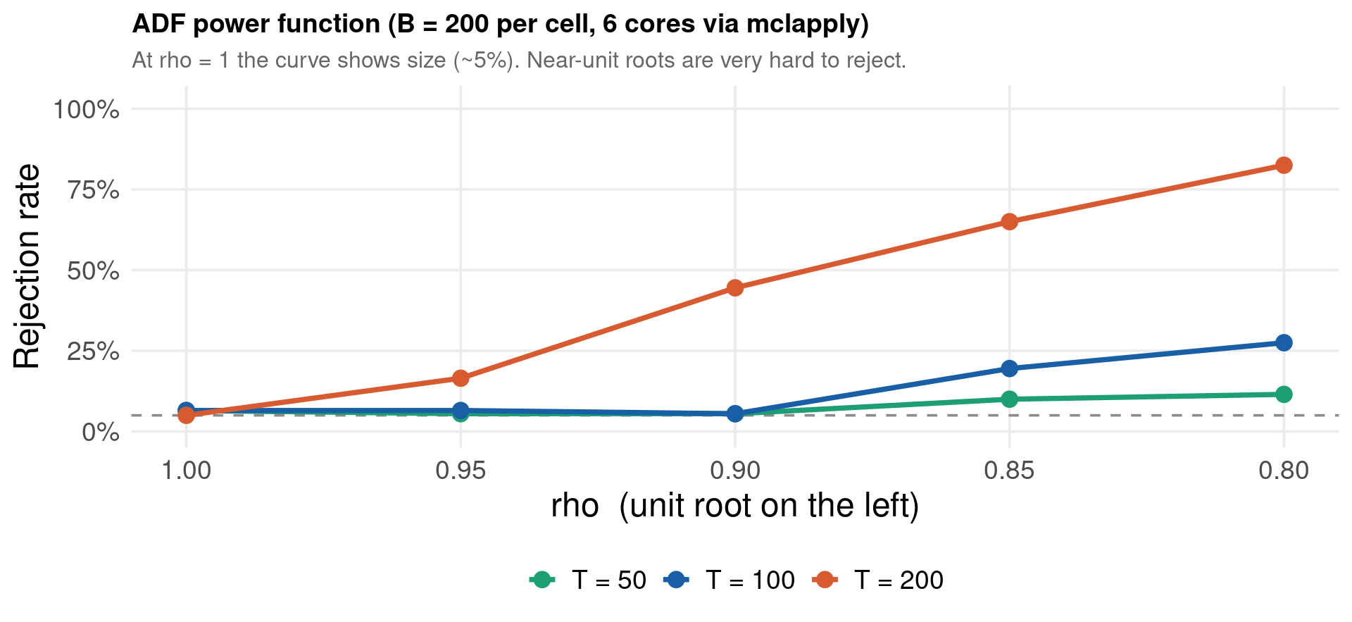
1. Grid: \(\rho \in \{0.80, 0.85, 0.90, 0.95, 1.00\}\) × \(T \in \{50, 100, 200\}\) — the \(\rho = 1\) row is the size row
2. Per cell: simulate an AR(1) with that \(\rho\), run the ADF test (adf.test / adfuller / dfuller), record whether \(p < 0.05\)
3. \(B = 200\) replications per cell (MC SE ≤ 0.035 — enough for the qualitative picture; scale up for research)
4. R distributes the 15 cells over 6 cores with mclapply — each adf.test() call costs ~2–5 ms, so this is exactly the task-size regime where parallelism pays
5. Read the surface: power rises as \(\rho\) falls and \(T\) grows; near the unit root (\(\rho = 0.95\)) power is painfully low even at \(T = 200\)

library(parallel)
library(tseries)

power_cell <- function(cell, B = 200) {
  rej <- 0L
  for (b in 1:B) {
    y <- numeric(cell$T)
    y[1] <- rnorm(1)
    for (t in 2:cell$T) y[t] <- cell$rho * y[t - 1] + rnorm(1)
    pv <- suppressWarnings(adf.test(y, alternative = "stationary")$p.value)
    rej <- rej + (pv < 0.05)
  }
  data.frame(rho = cell$rho, T = cell$T, power = rej / B)
}

grid <- expand.grid(rho = c(0.80, 0.85, 0.90, 0.95, 1.00), T = c(50, 100, 200))
cells <- lapply(seq_len(nrow(grid)), function(i) list(rho = grid$rho[i], T = grid$T[i]))

set.seed(14159)
pow <- do.call(rbind, mclapply(cells, power_cell, mc.set.seed = TRUE, mc.cores = 6))

pow$T_lab <- factor(paste0("T = ", pow$T), levels = paste0("T = ", c(50, 100, 200)))
ggplot(pow, aes(x = rho, y = power, color = T_lab, group = T_lab)) +
  geom_hline(yintercept = 0.05, linetype = "dashed", color = "grey55") +
  geom_line(linewidth = 1.3) + geom_point(size = 3.5) +
  scale_x_reverse() +
  scale_color_manual(values = c("#1D9E75", "#185FA5", "#D85A30"), name = NULL) +
  scale_y_continuous(labels = scales::percent_format(accuracy = 1), limits = c(0, 1.02)) +
  labs(x = "rho  (unit root on the left)", y = "Rejection rate",
       title = "ADF power function (B = 200 per cell, 6 cores via mclapply)",
       subtitle = "At rho = 1 the curve shows size (~5%). Near-unit roots are very hard to reject.") +
  theme_lecture

import numpy as np
import pandas as pd
from statsmodels.tsa.stattools import adfuller

rng = np.random.default_rng(14159)
B = 200

rows = []
for T in [50, 100, 200]:
    for rho in [0.80, 0.90, 0.95, 1.00]:
        rej = 0
        for b in range(B):
            e = rng.standard_normal(T)
            y = np.empty(T); y[0] = e[0]
            for t in range(1, T):
                y[t] = rho * y[t - 1] + e[t]
            pv = adfuller(y, regression="c", autolag="AIC")[1]
            rej += pv < 0.05
        rows.append({"T": T, "rho": rho, "power": rej / B})

tab = pd.DataFrame(rows).pivot(index="rho", columns="T", values="power")
print("ADF rejection rates (rho = 1.00 row = size):")

ADF rejection rates (rho = 1.00 row = size):

print(tab.round(3))

T       50     100    200
rho                      
0.80  0.340  0.825  0.990
0.90  0.275  0.350  0.810
0.95  0.100  0.150  0.325
1.00  0.110  0.040  0.055

capture program drop adfmc
program define adfmc, rclass
  syntax [, rho(real 1.0) tlen(integer 100)]
  clear
  quietly set obs `tlen'
  gen t = _n
  quietly tsset t
  gen y = rnormal() in 1
  quietly replace y = `rho'*L.y + rnormal() if t > 1
  quietly dfuller y
  return scalar rej = (r(Zt) < -2.86)     // 5% CV, drift case
end

set seed 14159
tempfile results
tempname h
postfile `h' rho power using `results'
foreach rho in 0.80 0.85 0.90 0.95 1.00 {
  quietly simulate rej = r(rej), reps(200) nodots: adfmc, rho(`rho') tlen(100)
  quietly summarize rej
  display "rho = `rho'   T = 100   rejection rate = " %6.3f r(mean)
  post `h' (`rho') (r(mean))
}
postclose `h'
display "rho = 1.00 is the size row: should be ~0.05."
use `results', clear
twoway (connected power rho, lcolor(navy) mcolor(navy) msize(medium)), ///
  yline(0.05, lpattern(dash) lcolor(gs10)) ///
  xscale(reverse) ylabel(0(0.2)1) ///
  xtitle("rho  (unit root on the left)") ytitle("Rejection rate") ///
  title("ADF power function at T = 100 (B = 200 per cell)")

rho = 0.80   T = 100   rejection rate =  0.840
rho = 0.85   T = 100   rejection rate =  0.615
rho = 0.90   T = 100   rejection rate =  0.300
rho = 0.95   T = 100   rejection rate =  0.095
rho = 1.00   T = 100   rejection rate =  0.025


rho = 1.00 is the size row: should be ~0.05.

Size Robustness — Stress-Testing the ADF Under Ugly Errors

• Setup

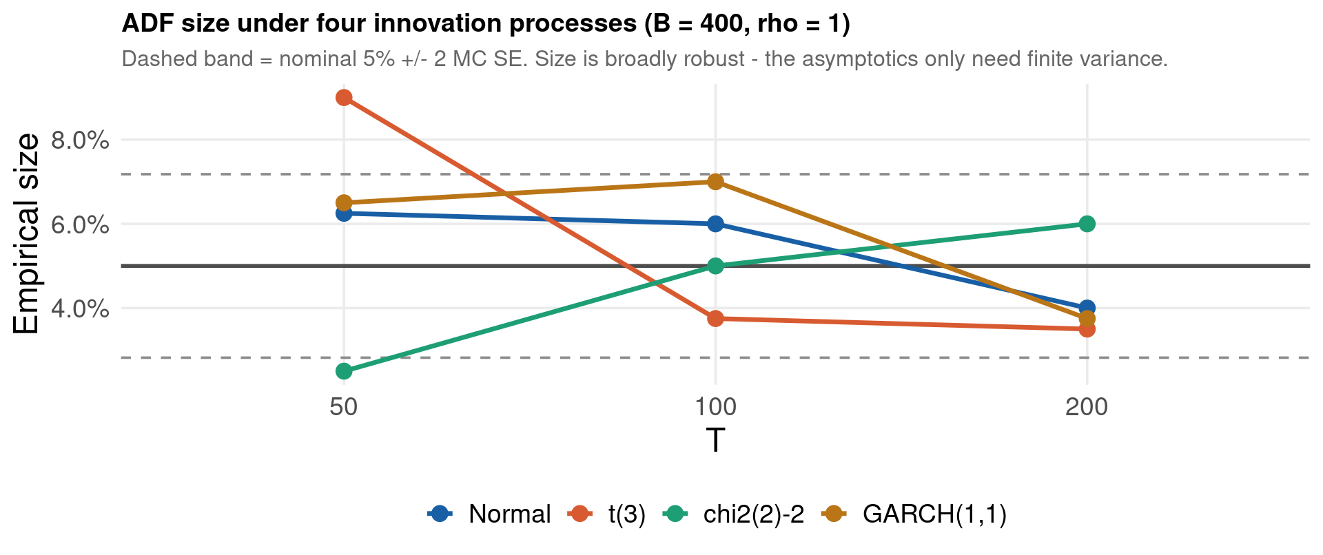
A good test keeps its size when the innovation distribution is not the Gaussian it was derived under. We re-run the size row (\(\rho = 1\), \(H_0\) true) with four innovation processes:

\[ \varepsilon_t \sim \mathcal{N}(0,1), \qquad \varepsilon_t \sim t(3), \qquad \varepsilon_t \sim \chi^2(2)-2, \qquad \varepsilon_t = \sigma_t z_t \ \text{(GARCH(1,1))} \]

\[ \sigma_t^2 = 0.1 + 0.3\,\varepsilon_{t-1}^2 + 0.6\,\sigma_{t-1}^2 \]

The Brownian-motion limit only needs finite variance and weak dependence, so size should survive — the question is how well at small T.

size_cell <- function(cell, B = 400) {
  rej <- 0L
  for (b in 1:B) {
    T_len <- cell$T
    eps <- numeric(T_len)
    if (cell$dist == "garch") {
      h <- 1
      for (t in 1:T_len) {
        z <- rnorm(1)
        eps[t] <- sqrt(h) * z
        h <- 0.1 + 0.3 * eps[t]^2 + 0.6 * h
      }
    } else {
      eps <- switch(cell$dist,
        normal = rnorm(T_len),
        t3     = rt(T_len, df = 3),
        chi2   = rchisq(T_len, df = 2) - 2)
    }
    y <- cumsum(eps)                       # random walk: H0 true
    pv <- suppressWarnings(adf.test(y, alternative = "stationary")$p.value)
    rej <- rej + (pv < 0.05)
  }
  data.frame(T = cell$T, dist = cell$dist, size = rej / B)
}

grid <- expand.grid(T = c(50, 100, 200), dist = c("normal", "t3", "chi2", "garch"),
                    stringsAsFactors = FALSE)
cells <- lapply(seq_len(nrow(grid)), function(i) list(T = grid$T[i], dist = grid$dist[i]))

set.seed(14159)
sz <- do.call(rbind, mclapply(cells, size_cell, mc.set.seed = TRUE, mc.cores = 6))
print(sz)

import numpy as np
import pandas as pd
from statsmodels.tsa.stattools import adfuller

rng = np.random.default_rng(14159)
B, T = 400, 100

def innovations(dist, T):
    if dist == "normal":
        return rng.standard_normal(T)
    if dist == "t3":
        return rng.standard_t(3, T)
    if dist == "chi2":
        return rng.chisquare(2, T) - 2
    eps = np.empty(T); h = 1.0
    for t in range(T):
        eps[t] = np.sqrt(h) * rng.standard_normal()
        h = 0.1 + 0.3 * eps[t]**2 + 0.6 * h
    return eps

rows = []
for dist in ["normal", "t3", "chi2", "garch"]:
    rej = 0
    for b in range(B):
        y = np.cumsum(innovations(dist, T))
        rej += adfuller(y, regression="c", autolag="AIC")[1] < 0.05
    rows.append({"dist": dist, "size": rej / B})
print(pd.DataFrame(rows).to_string(index=False))

  dist   size
normal 0.0575
    t3 0.0700
  chi2 0.0900
 garch 0.0975

print("Nominal 5%; MC SE ~ 0.011 at B = 400")

Nominal 5%; MC SE ~ 0.011 at B = 400

capture program drop adfsize
program define adfsize, rclass
  syntax [, dist(string)]
  clear
  quietly set obs 100
  gen t = _n
  quietly tsset t
  if "`dist'" == "t3"   gen eps = rt(3)
  else if "`dist'" == "chi2" gen eps = rchi2(2) - 2
  else gen eps = rnormal()
  gen y = sum(eps)
  quietly dfuller y
  return scalar rej = (r(Zt) < -2.86)
end

set seed 14159
tempfile results
tempname h
postfile `h' str8 dist size using `results'
foreach d in normal t3 chi2 {
  quietly simulate rej = r(rej), reps(300) nodots: adfsize, dist(`d')
  quietly summarize rej
  display "errors = `d'    empirical size = " %6.3f r(mean) "   (nominal 0.05)"
  post `h' ("`d'") (r(mean))
}
postclose `h'
use `results', clear
graph bar (asis) size, over(dist) yline(0.05, lcolor(red) lwidth(medthick)) ///
  bar(1, color(navy)) ytitle("Empirical size") ///
  title("ADF size under non-Gaussian errors (T = 100, rho = 1)")

errors = normal    empirical size =  0.057   (nominal 0.05)
errors = t3    empirical size =  0.050   (nominal 0.05)
errors = chi2    empirical size =  0.030   (nominal 0.05)

Part V: Applications in Micro & Macro

Measurement error · weak instruments · spurious regression · small-T bias

Micro I — Measurement Error and Attenuation Bias

• Setup

The classic labour-economics problem: true schooling \(x^*\) drives wages, but the survey records a noisy \(x = x^* + u\):

\[ y_i = \beta_0 + \beta_1 x_i^* + \varepsilon_i, \qquad x_i = x_i^* + u_i, \qquad u_i \perp (x_i^*, \varepsilon_i) \]

OLS of \(y\) on the observed \(x\) converges not to \(\beta_1\) but to a shrunken version:

\[ \text{plim}\ \hat\beta_1 = \beta_1 \cdot \lambda, \qquad \lambda = \frac{\sigma_{x^*}^2}{\sigma_{x^*}^2 + \sigma_u^2} \in (0, 1) \quad \text{(the reliability ratio)} \]

With \(\beta_1 = 2\), \(\sigma_{x^*}^2 = 1\), \(\sigma_u^2 = 0.5\): \(\text{plim}\ \hat\beta_1 = 2 \times \tfrac{1}{1.5} = [1.333]{.hl-red}\) — a 33% underestimate that no sample size can fix.

set.seed(14159)
B <- 2000
sigma_u2_grid <- c(0, 0.25, 0.5, 1)
n <- 500

results <- list()
for (s2 in sigma_u2_grid) {
  b1 <- numeric(B)
  for (b in 1:B) {
    xstar <- rnorm(n)
    x     <- xstar + rnorm(n, 0, sqrt(s2))
    y     <- 1 + 2 * xstar + rnorm(n)
    b1[b] <- coef(lm(y ~ x))[2]
  }
  results[[length(results) + 1]] <- tibble(
    sigma_u2 = s2, mean_b1 = mean(b1),
    theory = 2 * 1 / (1 + s2))
}
res_me <- bind_rows(results)
print(res_me)

ggplot(res_me, aes(x = sigma_u2)) +
  geom_hline(yintercept = 2, linetype = "dashed", color = "grey55") +
  geom_line(aes(y = theory, color = "Theory: 2 x reliability"), linewidth = 1.1, linetype = "dashed") +
  geom_point(aes(y = mean_b1, color = "MC mean of beta1-hat"), size = 4) +
  scale_color_manual(values = c("MC mean of beta1-hat" = "#185FA5",
                                "Theory: 2 x reliability" = "#D85A30"), name = NULL) +
  labs(x = "Measurement-error variance sigma_u^2", y = "E[beta1-hat]",
       title = "Attenuation bias: noisier regressors, smaller coefficients",
       subtitle = "True beta1 = 2 (grey dashed). MC dots land exactly on the reliability-ratio prediction.") +
  theme_lecture

# A tibble: 4 × 3
  sigma_u2 mean_b1 theory
     <dbl>   <dbl>  <dbl>
1     0       2.00   2   
2     0.25    1.60   1.6 
3     0.5     1.33   1.33
4     1       1.00   1   

import numpy as np

rng = np.random.default_rng(14159)
B, n = 2000, 500

print(f"{'sigma_u^2':>10} {'MC mean b1':>12} {'theory':>8}")

 sigma_u^2   MC mean b1   theory

for s2 in [0, 0.25, 0.5, 1]:
    b1 = np.empty(B)
    for b in range(B):
        xstar = rng.standard_normal(n)
        x = xstar + rng.normal(0, np.sqrt(s2), n)
        y = 1 + 2 * xstar + rng.standard_normal(n)
        b1[b] = np.cov(x, y)[0, 1] / x.var(ddof=1)
    print(f"{s2:>10} {b1.mean():>12.4f} {2 / (1 + s2):>8.4f}")

         0       2.0021   2.0000
      0.25       1.6006   1.6000
       0.5       1.3322   1.3333
         1       1.0000   1.0000

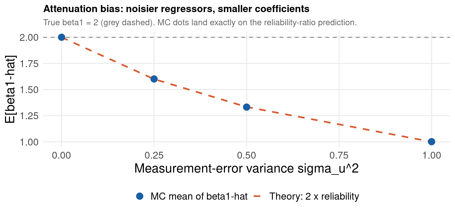
print("True beta1 = 2; the MC mean matches 2 x reliability ratio")

True beta1 = 2; the MC mean matches 2 x reliability ratio

capture program drop memc
program define memc, rclass
  syntax [, s2(real 0.5)]
  clear
  quietly set obs 500
  gen xstar = rnormal()
  gen u = rnormal()
  gen x = xstar + sqrt(`s2')*u        // sqrt(0)*u = 0 handles the no-noise case
  gen y = 1 + 2*xstar + rnormal()
  quietly regress y x
  return scalar b1 = _b[x]
end

set seed 14159
tempfile results
tempname h
postfile `h' s2 meanb1 theory using `results'
foreach s2 in 0 0.25 0.5 1 {
  quietly simulate b1 = r(b1), reps(1000) nodots: memc, s2(`s2')
  quietly summarize b1
  display "sigma_u^2 = `s2'   MC mean b1 = " %6.4f r(mean) ///
          "   theory = " %6.4f 2/(1 + `s2')
  post `h' (`s2') (r(mean)) (2/(1 + `s2'))
}
postclose `h'
use `results', clear
twoway (line theory s2, lcolor(red) lpattern(dash) lwidth(medthick)) ///
       (scatter meanb1 s2, mcolor(navy) msize(large)), ///
  yline(2, lpattern(dash) lcolor(gs10)) ///
  legend(order(2 "MC mean of b1" 1 "Theory: 2 x reliability")) ///
  xtitle("Measurement-error variance sigma_u^2") ytitle("E[b1]") ///
  title("Attenuation bias: noisier regressors, smaller coefficients")

  5.   post `h' (`s2') (r(mean)) (2/(1 + `s2'))
  6. }
sigma_u^2 = 0   MC mean b1 = 1.9991   theory = 2.0000
sigma_u^2 = 0.25   MC mean b1 = 1.5996   theory = 1.6000
sigma_u^2 = 0.5   MC mean b1 = 1.3363   theory = 1.3333
sigma_u^2 = 1   MC mean b1 = 1.0024   theory = 1.0000

Micro II — Weak Instruments

• Setup

IV fixes endogeneity — if the instrument is strong. The just-identified DGP:

\[ y_i = \beta x_i + \varepsilon_i, \qquad x_i = \pi z_i + v_i, \qquad \text{Corr}(\varepsilon_i, v_i) = 0.8, \qquad \beta = 1 \]

\[ \hat\beta_{2SLS} = \frac{\mathbf{z}'\mathbf{y}}{\mathbf{z}'\mathbf{x}}, \qquad \text{instrument strength} \approx \text{first-stage } F = \left(\frac{\hat\pi}{\text{SE}(\hat\pi)}\right)^2 \]

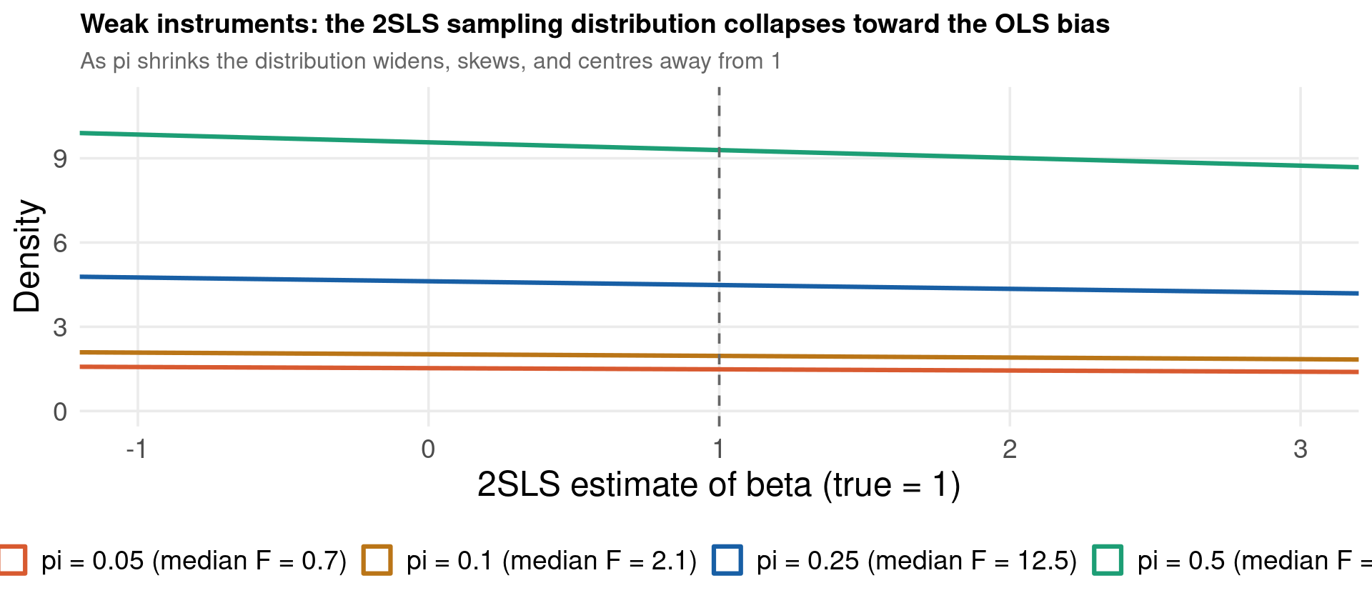
Staiger & Stock (1997): with weak \(\pi\), 2SLS is biased toward OLS and its distribution is wildly non-Normal. The famous rule of thumb — first-stage \(F > 10\) — comes straight from Monte Carlo evidence.

set.seed(14159)
B <- 2000; n <- 200
pi_grid <- c(0.05, 0.1, 0.25, 0.5)      # instrument strength

results <- list()
for (pi_z in pi_grid) {
  b_iv <- numeric(B); F1 <- numeric(B)
  for (b in 1:B) {
    z <- rnorm(n)
    err <- MASS::mvrnorm(n, c(0, 0), matrix(c(1, 0.8, 0.8, 1), 2, 2))
    v <- err[, 1]; e <- err[, 2]
    x <- pi_z * z + v
    y <- 1 * x + e
    b_iv[b] <- sum(z * y) / sum(z * x)
    fs      <- summary(lm(x ~ z))$coefficients
    F1[b]   <- (fs["z", "t value"])^2
  }
  results[[length(results) + 1]] <- tibble(
    pi = pi_z, median_F = median(F1),
    median_bias = median(b_iv) - 1,
    p10 = quantile(b_iv, 0.10), p90 = quantile(b_iv, 0.90),
    b_iv = list(b_iv))
}
res_iv <- bind_rows(results)
print(res_iv |> select(-b_iv))

df_dens <- res_iv |>
  select(pi, b_iv) |>
  unnest(b_iv) |>
  mutate(pi_lab = factor(glue("pi = {pi} (median F = {round(res_iv$median_F[match(pi, res_iv$pi)], 1)})")))

ggplot(df_dens, aes(x = b_iv, color = pi_lab)) +
  geom_density(linewidth = 1.1) +
  geom_vline(xintercept = 1, linetype = "dashed", color = "grey40") +
  coord_cartesian(xlim = c(-1, 3)) +
  scale_color_manual(values = c("#D85A30", "#BA7517", "#185FA5", "#1D9E75"), name = NULL) +
  labs(x = "2SLS estimate of beta (true = 1)", y = "Density",
       title = "Weak instruments: the 2SLS sampling distribution collapses toward the OLS bias",
       subtitle = "As pi shrinks the distribution widens, skews, and centres away from 1") +
  theme_lecture

   pi median_F median_bias    p10  p90
 0.05    0.717     0.46880 -0.502 3.38
 0.10    2.064     0.11549 -0.769 1.81
 0.25   12.452     0.00289  0.419 1.29
 0.50   49.801    -0.00261  0.777 1.16

import numpy as np

rng = np.random.default_rng(14159)
B, n = 2000, 200
cov = np.array([[1.0, 0.8], [0.8, 1.0]])

print(f"{'pi':>6} {'median F':>10} {'median bias':>12} {'10-90% range':>18}")

    pi   median F  median bias       10-90% range

for pi_z in [0.05, 0.1, 0.25, 0.5]:
    b_iv = np.empty(B); F1 = np.empty(B)
    for b in range(B):
        z = rng.standard_normal(n)
        err = rng.multivariate_normal([0, 0], cov, size=n)
        v, e = err[:, 0], err[:, 1]
        x = pi_z * z + v
        y = x + e
        b_iv[b] = (z @ y) / (z @ x)
        pi_hat = (z @ x) / (z @ z)
        resid = x - pi_hat * z
        se_pi = np.sqrt(resid @ resid / (n - 1) / (z @ z))
        F1[b] = (pi_hat / se_pi) ** 2
    p10, p90 = np.percentile(b_iv, [10, 90])
    print(f"{pi_z:>6} {np.median(F1):>10.1f} {np.median(b_iv) - 1:>12.3f} "
          f"[{p10:>7.2f}, {p90:>6.2f}]")

  0.05        0.8        0.469 [  -0.30,   3.28]
   0.1        2.0        0.123 [  -0.69,   1.76]
  0.25       12.4       -0.007 [   0.47,   1.28]
   0.5       49.1       -0.003 [   0.77,   1.15]

print("True beta = 1. Below F ~ 10 the 2SLS estimator is unusable.")

True beta = 1. Below F ~ 10 the 2SLS estimator is unusable.

capture program drop wivmc
program define wivmc, rclass
  syntax [, pi(real 0.5)]
  clear
  quietly set obs 200
  gen z = rnormal()
  gen v = rnormal()
  gen e = 0.8*v + sqrt(1 - 0.64)*rnormal()
  gen x = `pi'*z + v
  gen y = x + e
  quietly ivregress 2sls y (x = z)
  return scalar biv = _b[x]
  quietly regress x z
  return scalar F1 = e(F)
end

set seed 14159
tempfile all
local first = 1
foreach p in 0.05 0.25 0.5 {
  quietly simulate biv = r(biv) F1 = r(F1), reps(1000) nodots: wivmc, pi(`p')
  quietly summarize F1, detail
  local medF = r(p50)
  quietly summarize biv, detail
  display "pi = `p'   median F = " %6.1f `medF' ///
          "   median 2SLS bias = " %7.3f r(p50) - 1
  quietly gen double pi = `p'
  if `first' == 0 quietly append using `all'
  quietly save `all', replace
  local first = 0
}
use `all', clear
twoway (kdensity biv if pi == 0.5  & inrange(biv, -1, 3), lcolor(green) lwidth(medthick)) ///
       (kdensity biv if pi == 0.25 & inrange(biv, -1, 3), lcolor(navy) lwidth(medthick)) ///
       (kdensity biv if pi == 0.05 & inrange(biv, -1, 3), lcolor(red) lwidth(medthick)), ///
  xline(1, lpattern(dash) lcolor(gs8)) ///
  legend(label(1 "pi = 0.5 (strong)") label(2 "pi = 0.25") label(3 "pi = 0.05 (weak)")) ///
  xtitle("2SLS estimate of beta (true = 1)") ytitle("Density") ///
  title("Weak instruments push 2SLS toward the OLS bias")

  7.   quietly gen double pi = `p'
  8.   if `first' == 0 quietly append using `all'
  9.   quietly save `all', replace
 10.   local first = 0
 11. }
pi = 0.05   median F =    0.7   median 2SLS bias =   0.521
pi = 0.25   median F =   12.3   median 2SLS bias =   0.003
pi = 0.5   median F =   49.0   median 2SLS bias =  -0.007

(simulate: wivmc)

Macro I — Spurious Regression (Granger–Newbold)

• Setup

Regress one random walk on another, completely independent one:

\[ y_t = y_{t-1} + \varepsilon_t, \qquad x_t = x_{t-1} + u_t, \qquad \varepsilon_t \perp u_s \;\forall\, t, s \]

\[ y_t = a + b\,x_t + w_t \quad\text{— true } b = 0, \text{ yet…} \]

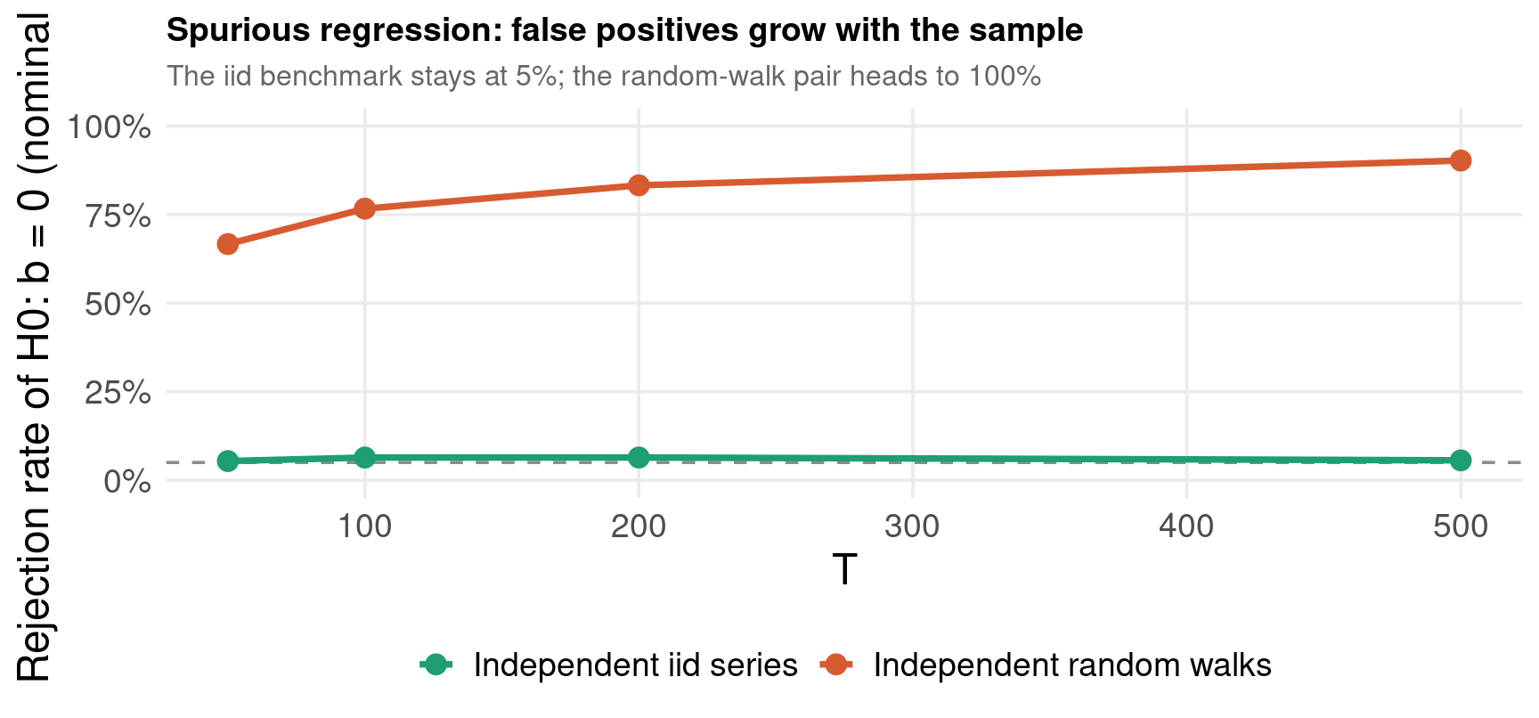
Granger & Newbold (1974) discovered by simulation that the \(t\)-test on \(b\) rejects far more than 5% — and Phillips (1986) later proved that the rejection rate tends to 1 as \(T \to \infty\). The MC came first; the theory followed twelve years later. Classic diagnostic: \(R^2 > DW\) signals a spurious regression.

set.seed(14159)
B <- 1000
T_grid <- c(50, 100, 200, 500)

rej_rw <- numeric(length(T_grid))
rej_iid <- numeric(length(T_grid))
for (j in seq_along(T_grid)) {
  T_len <- T_grid[j]
  r1 <- 0; r2 <- 0
  for (b in 1:B) {
    y <- cumsum(rnorm(T_len)); x <- cumsum(rnorm(T_len))
    p_rw <- summary(lm(y ~ x))$coefficients[2, 4]
    r1 <- r1 + (p_rw < 0.05)
    yi <- rnorm(T_len); xi <- rnorm(T_len)     # iid benchmark
    p_iid <- summary(lm(yi ~ xi))$coefficients[2, 4]
    r2 <- r2 + (p_iid < 0.05)
  }
  rej_rw[j] <- r1 / B; rej_iid[j] <- r2 / B
}

df_sp <- bind_rows(
  tibble(T = T_grid, rate = rej_rw,  case = "Independent random walks"),
  tibble(T = T_grid, rate = rej_iid, case = "Independent iid series"))
ggplot(df_sp, aes(x = T, y = rate, color = case)) +
  geom_hline(yintercept = 0.05, linetype = "dashed", color = "grey55") +
  geom_line(linewidth = 1.3) + geom_point(size = 3.5) +
  scale_color_manual(values = c("#1D9E75", "#D85A30"), name = NULL) +
  scale_y_continuous(labels = scales::percent_format(accuracy = 1), limits = c(0, 1)) +
  labs(x = "T", y = "Rejection rate of H0: b = 0 (nominal 5%)",
       title = "Spurious regression: false positives grow with the sample",
       subtitle = "The iid benchmark stays at 5%; the random-walk pair heads to 100%") +
  theme_lecture

import numpy as np
from scipy import stats

rng = np.random.default_rng(14159)
B = 1000

print(f"{'T':>5} {'reject rate (RW pair)':>22} {'reject rate (iid pair)':>23}")

    T  reject rate (RW pair)  reject rate (iid pair)

for T in [50, 100, 200, 500]:
    r_rw = 0; r_iid = 0
    for b in range(B):
        for kind in ["rw", "iid"]:
            if kind == "rw":
                y = np.cumsum(rng.standard_normal(T)); x = np.cumsum(rng.standard_normal(T))
            else:
                y = rng.standard_normal(T); x = rng.standard_normal(T)
            xc = x - x.mean(); yc = y - y.mean()
            bh = (xc @ yc) / (xc @ xc)
            resid = yc - bh * xc
            se = np.sqrt(resid @ resid / (T - 2) / (xc @ xc))
            rej = abs(bh / se) > stats.t.ppf(0.975, T - 2)
            if kind == "rw":
                r_rw += rej
            else:
                r_iid += rej
    print(f"{T:>5} {r_rw / B:>22.3f} {r_iid / B:>23.3f}")

   50                  0.649                   0.063
  100                  0.783                   0.053
  200                  0.859                   0.050
  500                  0.895                   0.041

print("Nominal level 5% - the random-walk pair over-rejects massively.")

Nominal level 5% - the random-walk pair over-rejects massively.

capture program drop spurmc
program define spurmc, rclass
  syntax [, tlen(integer 100)]
  clear
  quietly set obs `tlen'
  gen y = sum(rnormal())
  gen x = sum(rnormal())
  quietly regress y x
  return scalar rej = (abs(_b[x]/_se[x]) > invttail(`tlen' - 2, 0.025))
  return scalar r2  = e(r2)
end

set seed 14159
tempfile results
tempname h
postfile `h' T rate using `results'
foreach T in 50 100 200 500 {
  quietly simulate rej = r(rej) r2 = r(r2), reps(500) nodots: spurmc, tlen(`T')
  quietly summarize rej
  local rr = r(mean)
  quietly summarize r2
  display "T = " %4.0f `T' "   rejection rate = " %5.3f `rr' ///
          "   mean R2 = " %5.3f r(mean) "   (both should be ~0.05 if the test worked)"
  post `h' (`T') (`rr')
}
postclose `h'
use `results', clear
twoway (connected rate T, lcolor(red) mcolor(red) msize(medium)), ///
  yline(0.05, lpattern(dash) lcolor(gs10)) ylabel(0(0.2)1) ///
  xtitle("T") ytitle("Rejection rate of H0: b = 0 (nominal 5%)") ///
  title("Spurious regression: false positives grow with the sample")

  7.   post `h' (`T') (`rr')
  8. }
T =   50   rejection rate = 0.688   mean R2 = 0.241   (both should be ~0.05 if the test worked)
T =  100   rejection rate = 0.766   mean R2 = 0.231   (both should be ~0.05 if the test worked)
T =  200   rejection rate = 0.834   mean R2 = 0.242   (both should be ~0.05 if the test worked)
T =  500   rejection rate = 0.898   mean R2 = 0.255   (both should be ~0.05 if the test worked)

Macro II — Small-T Bias in Dynamic Models

• Setup

Estimating persistence — of inflation, output gaps, interest rates — means fitting an AR(1):

\[ y_t = \rho\, y_{t-1} + \varepsilon_t, \qquad \hat\rho_{OLS} = \frac{\sum_t y_{t-1} y_t}{\sum_t y_{t-1}^2} \]

OLS is consistent here but biased downward in finite T (the lagged regressor is only predetermined, not strictly exogenous). Kendall’s approximation:

\[ \mathbb{E}[\hat\rho] - \rho \;\approx\; -\frac{1 + 3\rho}{T} \]

• At \(T = 25\), \(\rho = 0.9\): bias \(\approx -0.15\) — the estimated half-life of a shock is less than half the truth
• The same mechanism scaled to panels is the Nickell bias that motivates Arellano–Bond GMM

set.seed(14159)
B <- 5000
T_grid <- c(25, 50, 100, 200)
rho <- 0.9

bias_mc <- numeric(length(T_grid))
for (j in seq_along(T_grid)) {
  T_len <- T_grid[j]
  rho_hat <- numeric(B)
  for (b in 1:B) {
    y <- numeric(T_len)
    y[1] <- rnorm(1) / sqrt(1 - rho^2)     # stationary start
    for (t in 2:T_len) y[t] <- rho * y[t - 1] + rnorm(1)
    rho_hat[b] <- sum(y[-T_len] * y[-1]) / sum(y[-T_len]^2)
  }
  bias_mc[j] <- mean(rho_hat) - rho
}

df_ar <- tibble(T = T_grid, mc = bias_mc, kendall = -(1 + 3 * rho) / T_grid)
print(df_ar)

ggplot(df_ar, aes(x = T)) +
  geom_hline(yintercept = 0, linetype = "dashed", color = "grey55") +
  geom_line(aes(y = kendall, color = "Kendall approximation -(1+3rho)/T"),
            linewidth = 1.1, linetype = "dashed") +
  geom_line(aes(y = mc, color = "Monte Carlo bias"), linewidth = 1.3) +
  geom_point(aes(y = mc), color = "#185FA5", size = 3.5) +
  scale_color_manual(values = c("Monte Carlo bias" = "#185FA5",
                                "Kendall approximation -(1+3rho)/T" = "#D85A30"), name = NULL) +
  labs(x = "T", y = "Bias of rho-hat (true rho = 0.9)",
       title = "Downward bias of OLS persistence estimates in short samples",
       subtitle = "Macro samples are short: 25 years of annual data means rho-hat ~ 0.75 when truth is 0.9") +
  theme_lecture

   T       mc kendall
  25 -0.05774 -0.1480
  50 -0.03376 -0.0740
 100 -0.01749 -0.0370
 200 -0.00887 -0.0185

import numpy as np

rng = np.random.default_rng(14159)
B, rho = 5000, 0.9

print(f"{'T':>5} {'MC bias':>10} {'Kendall -(1+3rho)/T':>20}")

    T    MC bias  Kendall -(1+3rho)/T

for T in [25, 50, 100, 200]:
    rho_hat = np.empty(B)
    for b in range(B):
        y = np.empty(T)
        y[0] = rng.standard_normal() / np.sqrt(1 - rho**2)
        e = rng.standard_normal(T)
        for t in range(1, T):
            y[t] = rho * y[t - 1] + e[t]
        rho_hat[b] = (y[:-1] @ y[1:]) / (y[:-1] @ y[:-1])
    print(f"{T:>5} {rho_hat.mean() - rho:>10.4f} {-(1 + 3*rho)/T:>20.4f}")

   25    -0.0593              -0.1480
   50    -0.0339              -0.0740
  100    -0.0169              -0.0370
  200    -0.0091              -0.0185

capture program drop ar1mc
program define ar1mc, rclass
  syntax [, tlen(integer 50)]
  clear
  quietly set obs `tlen'
  gen t = _n
  quietly tsset t
  gen y = rnormal()/sqrt(1 - 0.81) in 1
  quietly replace y = 0.9*L.y + rnormal() if t > 1
  quietly regress y L.y, noconstant
  return scalar rho = _b[L.y]
end

set seed 14159
tempfile results
tempname h
postfile `h' T bias kendall using `results'
foreach T in 25 50 100 200 {
  quietly simulate rho = r(rho), reps(2000) nodots: ar1mc, tlen(`T')
  quietly summarize rho
  display "T = " %4.0f `T' "   MC bias = " %7.4f r(mean) - 0.9 ///
          "   Kendall = " %7.4f -(1 + 3*0.9)/`T'
  post `h' (`T') (r(mean) - 0.9) (-(1 + 3*0.9)/`T')
}
postclose `h'
use `results', clear
twoway (line kendall T, lcolor(red) lpattern(dash) lwidth(medthick)) ///
       (connected bias T, lcolor(navy) mcolor(navy) msize(medium)), ///
  yline(0, lpattern(dash) lcolor(gs10)) ///
  legend(order(2 "Monte Carlo bias" 1 "Kendall: -(1+3rho)/T")) ///
  xtitle("T") ytitle("Bias of rho-hat (true rho = 0.9)") ///
  title("Downward bias of OLS persistence estimates in short samples")

  5.   post `h' (`T') (r(mean) - 0.9) (-(1 + 3*0.9)/`T')
  6. }
T =   25   MC bias = -0.0538   Kendall = -0.1480
T =   50   MC bias = -0.0296   Kendall = -0.0740
T =  100   MC bias = -0.0153   Kendall = -0.0370
T =  200   MC bias = -0.0083   Kendall = -0.0185

Part VI: Applications in Finance

Option pricing · variance reduction · Value-at-Risk & Expected Shortfall

Pricing by Simulation — Geometric Brownian Motion

• The Model
• Algorithm
• Paths

Under the risk-neutral measure, the stock follows geometric Brownian motion:

\[ dS_t = r\,S_t\,dt + \sigma\,S_t\,dW_t \quad\Longrightarrow\quad S_T = S_0 \exp\!\left[\left(r - \tfrac{\sigma^2}{2}\right)T + \sigma\sqrt{T}\,Z\right], \quad Z \sim \mathcal{N}(0,1) \]

A European call with strike \(K\) pays \(\max(S_T - K, 0)\) at maturity; its price is a discounted expectation — exactly the object MC estimates:

\[ C = e^{-rT}\,\mathbb{E}^{\mathbb{Q}}\!\left[\max(S_T - K,\ 0)\right] \;\approx\; \frac{e^{-rT}}{B}\sum_{b=1}^{B} \max\!\left(S_T^{(b)} - K,\ 0\right) \]

For this payoff Black–Scholes gives the closed form to check against:

\[ C_{BS} = S_0\,\Phi(d_1) - K e^{-rT}\,\Phi(d_2), \qquad d_{1,2} = \frac{\ln(S_0/K) + (r \pm \sigma^2/2)T}{\sigma\sqrt{T}} \]

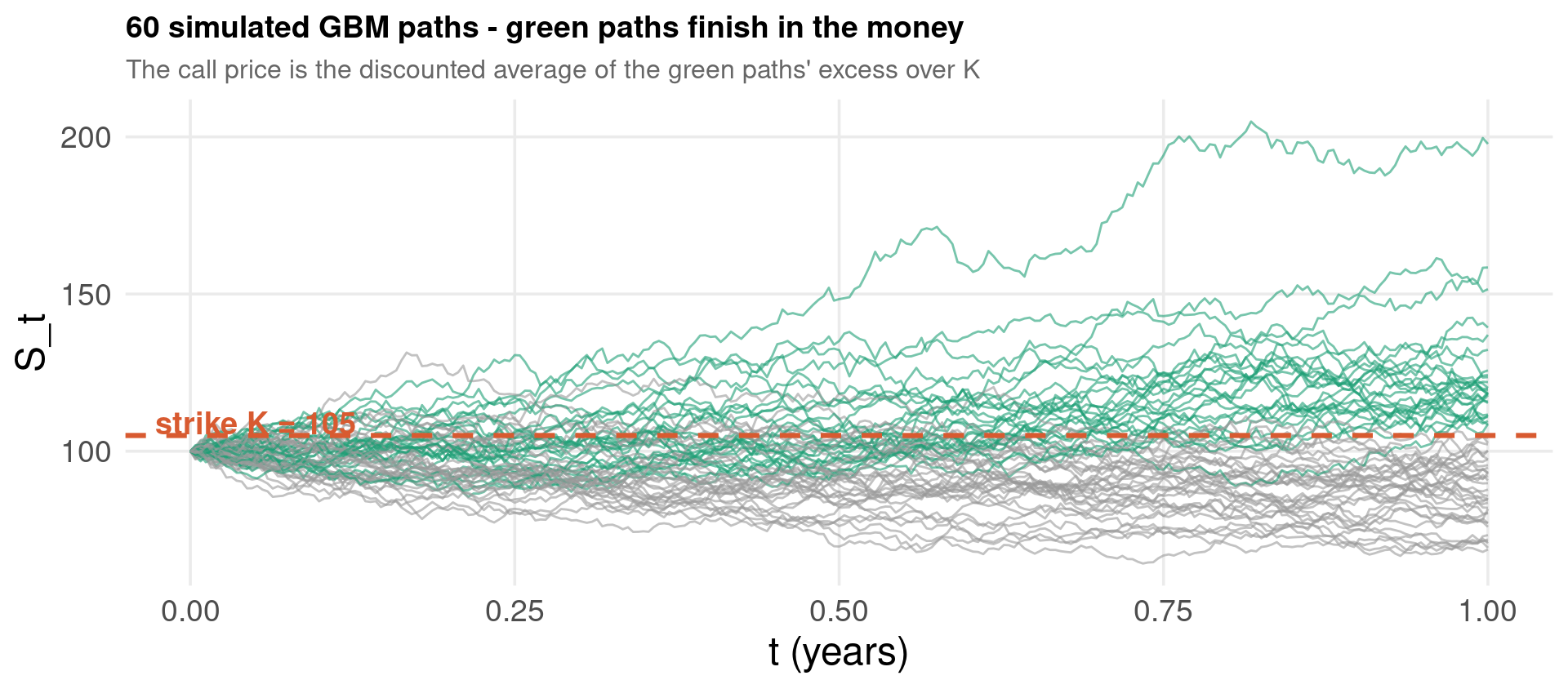
Parameters throughout: \(S_0 = 100\), \(K = 105\), \(r = 0.03\), \(\sigma = 0.2\), \(T = 1\). Boyle (1977) introduced this method precisely because most exotic payoffs have no closed form — MC is then the only general pricing tool.

1. Draw \(Z_b \sim \mathcal{N}(0,1)\) and form the terminal price \(S_T^{(b)} = S_0\, e^{(r - \sigma^2/2)T + \sigma\sqrt{T} Z_b}\)
2. Compute the discounted payoff \(e^{-rT}\max(S_T^{(b)} - K, 0)\)
3. Average over \(b = 1, \dots, B\); report the MC standard error \(\hat\sigma_{\text{payoff}}/\sqrt{B}\)
4. Variance reduction — antithetic variates: reuse every draw as \(-Z_b\); the pair’s payoffs are negatively correlated, so their average has lower variance at the same cost
5. Compare against \(C_{BS}\)

Why antithetic variates work

For a pair \((h(Z), h(-Z))\) the variance of the average is

\[ \text{Var}\!\left(\frac{h(Z) + h(-Z)}{2}\right) = \frac{\text{Var}(h)}{2}\left(1 + \text{Corr}\big(h(Z), h(-Z)\big)\right) \]

If \(h\) is monotone in \(Z\) (a call payoff is), the correlation is negative, so the paired estimator beats two independent draws — same number of random numbers, strictly smaller MC error. Other classical tricks in the same family: control variates (use a correlated payoff with known price), importance sampling (oversample the tail that matters), quasi-Monte Carlo (low-discrepancy sequences).

set.seed(14159)
S0 <- 100; K <- 105; r <- 0.03; sigma <- 0.2; T_mat <- 1
B <- 100000

# Black-Scholes closed form
d1 <- (log(S0 / K) + (r + sigma^2 / 2) * T_mat) / (sigma * sqrt(T_mat))
d2 <- d1 - sigma * sqrt(T_mat)
C_bs <- S0 * pnorm(d1) - K * exp(-r * T_mat) * pnorm(d2)

# Plain Monte Carlo
z  <- rnorm(B)
ST <- S0 * exp((r - sigma^2 / 2) * T_mat + sigma * sqrt(T_mat) * z)
payoff <- exp(-r * T_mat) * pmax(ST - K, 0)
C_mc  <- mean(payoff)
se_mc <- sd(payoff) / sqrt(B)

# Antithetic variates: reuse each z as -z (same B random numbers)
ST_a <- S0 * exp((r - sigma^2 / 2) * T_mat + sigma * sqrt(T_mat) * (-z))
payoff_a <- (payoff + exp(-r * T_mat) * pmax(ST_a - K, 0)) / 2
C_av  <- mean(payoff_a)
se_av <- sd(payoff_a) / sqrt(B)

cat(sprintf("Black-Scholes closed form : %.4f\n", C_bs))
cat(sprintf("Plain MC (B = 100000)     : %.4f   (SE %.4f)\n", C_mc, se_mc))
cat(sprintf("Antithetic MC             : %.4f   (SE %.4f)\n", C_av, se_av))
cat(sprintf("Variance reduction factor : %.1fx\n", (se_mc / se_av)^2))

Black-Scholes closed form : 7.1281

Plain MC (B = 100000)     : 7.1206   (SE 0.0396)

Antithetic MC             : 7.1478   (SE 0.0232)

Variance reduction factor : 2.9x

set.seed(14159)
n_steps <- 252; n_paths <- 60
dt <- T_mat / n_steps
paths <- matrix(NA_real_, n_steps + 1, n_paths)
paths[1, ] <- S0
for (p in 1:n_paths) {
  for (t in 2:(n_steps + 1)) {
    paths[t, p] <- paths[t - 1, p] * exp((r_f - sigma_f^2 / 2) * dt + sigma_f * sqrt(dt) * rnorm(1))
  }
}
df_paths <- as_tibble(paths, .name_repair = ~paste0("p", seq_along(.x))) |>
  mutate(t = (0:n_steps) / n_steps) |>
  pivot_longer(-t, names_to = "path", values_to = "S")
df_paths$itm <- df_paths$path %in% paste0("p", which(paths[n_steps + 1, ] > K))
ggplot(df_paths, aes(x = t, y = S, group = path, color = itm)) +
  geom_line(alpha = 0.6, linewidth = 0.5) +
  geom_hline(yintercept = K, color = "#D85A30", linewidth = 1.1, linetype = "dashed") +
  annotate("text", x = 0.05, y = K + 4, label = "strike K = 105", color = "#D85A30", size = 5, fontface = "bold") +
  scale_color_manual(values = c("grey60", "#1D9E75"), guide = "none") +
  labs(x = "t (years)", y = "S_t",
       title = "60 simulated GBM paths - green paths finish in the money",
       subtitle = "The call price is the discounted average of the green paths' excess over K") +
  theme_lecture

import numpy as np
from scipy import stats

rng = np.random.default_rng(14159)
S0, K, r, sigma, T = 100, 105, 0.03, 0.2, 1
B = 100000

d1 = (np.log(S0 / K) + (r + sigma**2 / 2) * T) / (sigma * np.sqrt(T))
d2 = d1 - sigma * np.sqrt(T)
C_bs = S0 * stats.norm.cdf(d1) - K * np.exp(-r * T) * stats.norm.cdf(d2)

z = rng.standard_normal(B)
ST = S0 * np.exp((r - sigma**2 / 2) * T + sigma * np.sqrt(T) * z)
payoff = np.exp(-r * T) * np.maximum(ST - K, 0)
C_mc, se_mc = payoff.mean(), payoff.std(ddof=1) / np.sqrt(B)

ST_a = S0 * np.exp((r - sigma**2 / 2) * T - sigma * np.sqrt(T) * z)
payoff_av = (payoff + np.exp(-r * T) * np.maximum(ST_a - K, 0)) / 2
C_av, se_av = payoff_av.mean(), payoff_av.std(ddof=1) / np.sqrt(B)

print(f"Black-Scholes closed form : {C_bs:.4f}")

Black-Scholes closed form : 7.1281

print(f"Plain MC (B = 100000)     : {C_mc:.4f}   (SE {se_mc:.4f})")

Plain MC (B = 100000)     : 7.1172   (SE 0.0395)

print(f"Antithetic MC             : {C_av:.4f}   (SE {se_av:.4f})")

Antithetic MC             : 7.1001   (SE 0.0229)

print(f"Variance reduction factor : {(se_mc / se_av)**2:.1f}x")

Variance reduction factor : 3.0x

quietly {
  clear
  set seed 14159
  set obs 100000
  scalar S0 = 100
  scalar K  = 105
  scalar r  = 0.03
  scalar sg = 0.2
  scalar T  = 1
  gen z  = rnormal()
  gen ST = S0 * exp((r - sg^2/2)*T + sg*sqrt(T)*z)
  gen payoff = exp(-r*T) * max(ST - K, 0)
  summarize payoff
  scalar C_mc  = r(mean)
  scalar se_mc = r(sd)/sqrt(_N)
  scalar d1 = (ln(S0/K) + (r + sg^2/2)*T) / (sg*sqrt(T))
  scalar d2 = d1 - sg*sqrt(T)
  scalar C_bs = S0*normal(d1) - K*exp(-r*T)*normal(d2)
}
display "Black-Scholes closed form : " %7.4f C_bs
display "Monte Carlo (B = 100000)  : " %7.4f C_mc "   (SE " %6.4f se_mc ")"

Black-Scholes closed form :  7.1281

Monte Carlo (B = 100000)  :  7.1863   (SE 0.0399)

Value-at-Risk and Expected Shortfall by Simulation

• Setup

For a portfolio with return \(R\), the level-\(\alpha\) Value-at-Risk and Expected Shortfall are

\[ \text{VaR}_\alpha = -\,q_\alpha(R), \qquad \text{ES}_\alpha = -\,\mathbb{E}\!\left[R \mid R \le q_\alpha(R)\right] \]

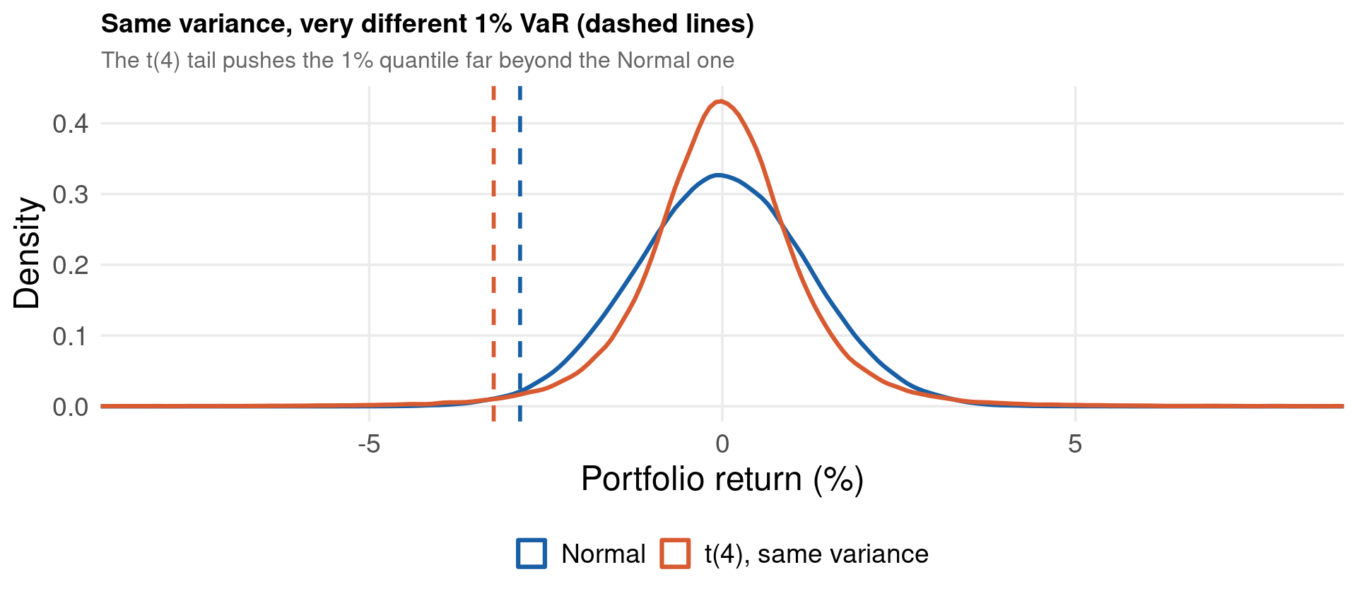
Simulation estimates both by reading quantiles and tail means off B simulated returns. The experiment: a two-asset portfolio (60/40, correlation 0.3, both with daily volatility 1.5%), returns drawn either Normal or Student-\(t(4)\) scaled to the same variance:

\[ R = 0.6\,r_1 + 0.4\,r_2 \]

• The Normal model underestimates tail risk: same variance, but \(t(4)\) tails hold far more mass beyond the 1% quantile
• ES reacts more strongly than VaR — it looks into the tail, not just at its edge; this is why Basel moved from VaR to ES

set.seed(14159)
B <- 200000
w <- c(0.6, 0.4); vol <- 0.015; rho_a <- 0.3
Sigma <- vol^2 * matrix(c(1, rho_a, rho_a, 1), 2, 2)

# Normal returns
rets_n <- MASS::mvrnorm(B, mu = c(0, 0), Sigma = Sigma)
R_n <- rets_n %*% w

# t(4) returns scaled to the same covariance: multiply by sqrt((nu-2)/nu) adjustment
nu <- 4
chi <- sqrt(rchisq(B, nu) / nu)
rets_t <- (MASS::mvrnorm(B, mu = c(0, 0), Sigma = Sigma * (nu - 2) / nu)) / chi
R_t <- rets_t %*% w

risk <- function(R, a) {
  q <- quantile(R, a)
  c(VaR = -q, ES = -mean(R[R <= q]))
}
for (a in c(0.05, 0.01)) {
  rn <- risk(R_n, a); rt <- risk(R_t, a)
  cat(sprintf("alpha = %d%%:  Normal VaR %.3f%%  ES %.3f%%   |   t(4) VaR %.3f%%  ES %.3f%%\n",
      round(100 * a), 100 * rn["VaR"], 100 * rn["ES"], 100 * rt["VaR"], 100 * rt["ES"]))
}

df_var <- bind_rows(tibble(R = as.numeric(R_n), model = "Normal"),
                    tibble(R = as.numeric(R_t), model = "t(4), same variance"))
ggplot(df_var, aes(x = 100 * R, color = model)) +
  geom_density(linewidth = 1.1) +
  geom_vline(xintercept = 100 * quantile(R_n, 0.01), color = "#185FA5", linetype = "dashed", linewidth = 1) +
  geom_vline(xintercept = 100 * quantile(R_t, 0.01), color = "#D85A30", linetype = "dashed", linewidth = 1) +
  coord_cartesian(xlim = c(-8, 8)) +
  scale_color_manual(values = c("#185FA5", "#D85A30"), name = NULL) +
  labs(x = "Portfolio return (%)", y = "Density",
       title = "Same variance, very different 1% VaR (dashed lines)",
       subtitle = "The t(4) tail pushes the 1% quantile far beyond the Normal one") +
  theme_lecture

alpha = 5%:  Normal VaR 2.021%  ES 2.537%   |   t(4) VaR 1.838%  ES 2.769%
alpha = 1%:  Normal VaR 2.864%  ES 3.295%   |   t(4) VaR 3.237%  ES 4.519%

import numpy as np

rng = np.random.default_rng(14159)
B = 200000
w = np.array([0.6, 0.4]); vol = 0.015; rho = 0.3
Sigma = vol**2 * np.array([[1, rho], [rho, 1]])

R_n = rng.multivariate_normal([0, 0], Sigma, size=B) @ w

nu = 4
chi = np.sqrt(rng.chisquare(nu, B) / nu)
R_t = (rng.multivariate_normal([0, 0], Sigma * (nu - 2) / nu, size=B) / chi[:, None]) @ w

def risk(R, a):
    q = np.quantile(R, a)
    return -q, -R[R <= q].mean()

for a in [0.05, 0.01]:
    vn, en = risk(R_n, a)
    vt, et = risk(R_t, a)
    print(f"alpha = {a:.0%}:  Normal VaR {vn:.3%}  ES {en:.3%}   |   "
          f"t(4) VaR {vt:.3%}  ES {et:.3%}")

alpha = 5%:  Normal VaR 2.007%  ES 2.520%   |   t(4) VaR 1.837%  ES 2.782%
alpha = 1%:  Normal VaR 2.844%  ES 3.262%   |   t(4) VaR 3.267%  ES 4.564%

print("Fat tails: identical variance, much larger 1% VaR and ES.")

Fat tails: identical variance, much larger 1% VaR and ES.

quietly {
  clear
  set seed 14159
  set obs 200000
  * two correlated normals via Cholesky: r2 = rho*r1 + sqrt(1-rho^2)*z2
  gen z1 = rnormal()
  gen z2 = 0.3*z1 + sqrt(1 - 0.09)*rnormal()
  gen r1n = 0.015*z1
  gen r2n = 0.015*z2
  gen Rn  = 0.6*r1n + 0.4*r2n
  * t(4) version, scaled to the same variance
  gen chi = sqrt(rchi2(4)/4)
  gen Rt  = (0.6*0.015*sqrt(0.5)*z1 + 0.4*0.015*sqrt(0.5)*z2) / chi
  _pctile Rn, percentiles(1 5)
  scalar vn1 = -r(r1)
  scalar vn5 = -r(r2)
  _pctile Rt, percentiles(1 5)
  scalar vt1 = -r(r1)
  scalar vt5 = -r(r2)
}
display "Normal:  5% VaR = " %6.3f 100*vn5 "%   1% VaR = " %6.3f 100*vn1 "%"
display "t(4)  :  5% VaR = " %6.3f 100*vt5 "%   1% VaR = " %6.3f 100*vt1 "%"
display "Same variance, but the fat-tailed 1% VaR is much larger."
quietly gen Rn_pct = 100*Rn
quietly gen Rt_pct = 100*Rt
local qn1 = -100*vn1
local qt1 = -100*vt1
twoway (kdensity Rn_pct if inrange(Rn_pct, -8, 8), lcolor(navy) lwidth(medthick)) ///
       (kdensity Rt_pct if inrange(Rt_pct, -8, 8), lcolor(red) lwidth(medthick)), ///
  xline(`qn1', lcolor(navy) lpattern(dash)) xline(`qt1', lcolor(red) lpattern(dash)) ///
  legend(label(1 "Normal") label(2 "t(4), same variance")) ///
  xtitle("Portfolio return (%)") ytitle("Density") ///
  title("Same variance, very different 1% VaR (dashed lines)")

Normal:  5% VaR =  2.015%   1% VaR =  2.844%

t(4)  :  5% VaR =  1.836%   1% VaR =  3.228%

Same variance, but the fat-tailed 1% VaR is much larger.

Exercises — Estimation

1. Modify the Part I π-estimator to compute \(\int_0^1 e^{-x^2}\,dx\) by MC and report the estimate with its MC standard error at \(B = 10^4\) and \(B = 10^6\). Verify the 1/√B law between the two runs.
2. In the CLT laboratory, replace \(\text{Exp}(1)\) with \(\text{Bernoulli}(0.05)\) (rare events). How large must \(n\) be before the histogram of \(Z_n\) looks Normal? Relate your answer to the Berry–Esseen bound with \(\rho = p(1-p)\left[(1-p)^2 + p^2\right]\).
3. Extend the OLS study with a fourth error distribution, \(\varepsilon \sim \text{Exp}(1) - 1\), and a lognormal regressor \(x_1 = e^{Z}\). Which change damages t-test size more — skewed errors or a skewed regressor?
4. In the measurement-error slide, add classical measurement error to \(y\) instead of \(x\). Show by simulation that the slope stays unbiased and explain why only the standard errors grow.
5. Reproduce the weak-IV densities with 3 instruments instead of 1 (2SLS with over-identification). Does the median bias at \(\pi = 0.05\) get better or worse as instruments are added?
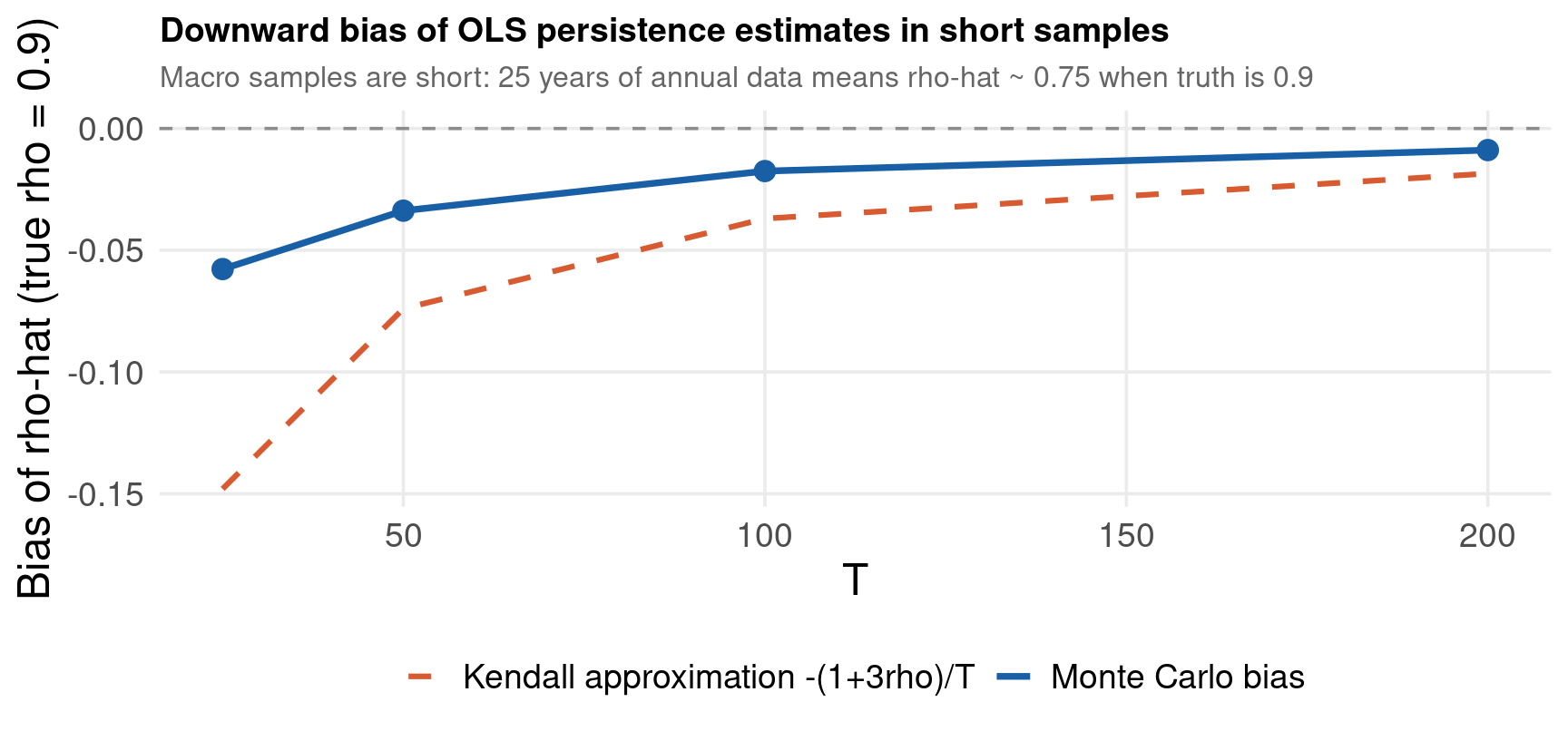
6. In the AR(1) bias study, apply the analytical correction \(\tilde\rho = \hat\rho + (1 + 3\hat\rho)/T\) and re-compute the bias. How much of the distortion does the first-order correction remove at \(T = 25\)?
7. Price an Asian call (payoff on the average price over 12 monthly observations) by simulating full GBM paths. There is no closed form — report the MC price, its SE, and the antithetic-variates improvement.

Exercises — Testing

1. Rebuild the Dickey–Fuller critical values for the no-constant case \(\Delta y_t = \gamma y_{t-1} + \varepsilon_t\) and for the trend case. Compare your 5% quantiles with MacKinnon’s \(-1.95\) and \(-3.41\).
2. Simulate the size of the naive strategy “use \(\pm 1.96\) Normal critical values for the ADF \(\tau\)”. How many true unit roots does it wrongly reject at \(T = 100\)?
3. Estimate the ADF power against the local alternative \(\rho_T = 1 - c/T\) for \(c \in \{5, 10, 20\}\) and \(T \in \{100, 200, 400\}\). Confirm that power depends on \(c\) but not on \(T\) — the Pitman-drift signature.
4. Compare ADF and KPSS by simulation: for \(\rho \in \{0.9, 0.95, 1\}\), tabulate both tests’ rejection rates and show they make opposite errors near the unit root.
5. Design your own test: propose a statistic for \(H_0\!: \text{median}(X) = 0\) based on the sign of the sample median, simulate its distribution under the null for \(n = 25\), extract 5% critical values, then estimate its power against a shifted \(t(3)\) alternative. Compare with the standard \(t\)-test.
6. In the spurious-regression study, add a lagged dependent variable to the regression (\(y_t\) on \(y_{t-1}\) and \(x_t\)). Show by simulation that the over-rejection largely disappears and explain why.
7. Compute the size of the heteroskedasticity study’s classical \(t\)-test as the heteroskedasticity strength varies: \(\varepsilon_i = e^{\kappa x_i} u_i\) for \(\kappa \in \{0, 0.25, 0.5, 1\}\). Plot size against \(\kappa\) for classical and HC3 standard errors.

Further Reading

• Methodology
• Tests & Time Series
• Finance

• Metropolis, N., & Ulam, S. (1949). The Monte Carlo method. JASA, 44(247), 335–341. DOI: 10.1080/01621459.1949.10483310
• Hendry, D. F. (1984). Monte Carlo experimentation in econometrics. Handbook of Econometrics, Vol. 2. DOI: 10.1016/S1573-4412(84)01012-8
• Kiviet, J. F. (2012). Monte Carlo Simulation for Econometricians. DOI: 10.1561/0800000011
• Davidson, R., & MacKinnon, J. G. (2004). Econometric Theory and Methods, Ch. 21. Oxford University Press.
• Efron, B., & Hastie, T. (2016). Computer Age Statistical Inference. Cambridge University Press. DOI: 10.1017/CBO9781316576533
• L’Ecuyer, P., & Simard, R. (2007). TestU01: a C library for empirical testing of random number generators. ACM TOMS, 33(4). DOI: 10.1145/1268776.1268777

• Dickey, D. A., & Fuller, W. A. (1979). JASA, 74(366), 427–431. DOI: 10.1080/01621459.1979.10482531
• MacKinnon, J. G. (1996). Numerical distribution functions for unit root and cointegration tests. Journal of Applied Econometrics, 11(6), 601–618. DOI: 10.1002/(SICI)1099-1255(199611)11:6<601::AID-JAE417>3.0.CO;2-T
• Granger, C. W. J., & Newbold, P. (1974). Spurious regressions in econometrics. Journal of Econometrics, 2(2), 111–120. DOI: 10.1016/0304-4076(74)90034-7
• Phillips, P. C. B. (1986). Understanding spurious regressions in econometrics. Journal of Econometrics, 33(3), 311–340. DOI: 10.1016/0304-4076(86)90001-1
• Elliott, G., Rothenberg, T. J., & Stock, J. H. (1996). Efficient tests for an autoregressive unit root. Econometrica, 64(4), 813–836. DOI: 10.2307/2171846
• Staiger, D., & Stock, J. H. (1997). Instrumental variables regression with weak instruments. Econometrica, 65(3), 557–586. DOI: 10.2307/2171753
• Nickell, S. (1981). Biases in dynamic models with fixed effects. Econometrica, 49(6), 1417–1426. DOI: 10.2307/1911408

• Boyle, P. P. (1977). Options: a Monte Carlo approach. Journal of Financial Economics, 4(3), 323–338. DOI: 10.1016/0304-405X(77)90005-8
• Glasserman, P. (2003). Monte Carlo Methods in Financial Engineering. Springer. DOI: 10.1007/978-0-387-21617-1
• Black, F., & Scholes, M. (1973). The pricing of options and corporate liabilities. Journal of Political Economy, 81(3), 637–654. DOI: 10.1086/260062
• Longstaff, F. A., & Schwartz, E. S. (2001). Valuing American options by simulation. Review of Financial Studies, 14(1), 113–147. DOI: 10.1093/rfs/14.1.113
• Artzner, P., Delbaen, F., Eber, J.-M., & Heath, D. (1999). Coherent measures of risk. Mathematical Finance, 9(3), 203–228. DOI: 10.1111/1467-9965.00068
• McNeil, A. J., Frey, R., & Embrechts, P. (2015). Quantitative Risk Management, 2nd ed. Princeton University Press.

Thank You

Athanassios Stavrakoudis

Applied Informatics and Computational Economics Lab
Department of Economics
University of Ioannina, Greece

astavrak@uoi.gr · linkedin.com/in/astavrakoudis