Networks and Trade Analysis

Examples and Applications using &

Applied Informatics and Computational Economics Lab

2 July 2026

Required Packages

library(tidyverse)    # data wrangling + ggplot2
library(igraph)       # graphs, centrality, communities, random graphs
library(ggraph)       # network visualization, grammar-of-graphics style
library(tidygraph)    # tidy interface to igraph
library(kableExtra)   # results tables
# optional, for downloading the raw data yourself:
# library(eurostat)   # get_eurostat("ext_tec03")
import pandas as pd
import numpy as np
import networkx as nx            # graphs, centrality, communities
import matplotlib.pyplot as plt

Literature Review — Networks in Economics

  • Jackson (2008), Social and Economic Networks, Princeton University Press — the canonical graduate text. doi:10.2307/j.ctvcm4gh1
  • Jackson, Rogers & Zenou (2017), “The Economic Consequences of Social-Network Structure”, Journal of Economic Literature 55(1), 49–95. doi:10.1257/jel.20150694
  • Acemoglu, Carvalho, Ozdaglar & Tahbaz-Salehi (2012), “The Network Origins of Aggregate Fluctuations”, Econometrica 80(5), 1977–2016. doi:10.3982/ECTA9623
  • Carvalho (2014), “From Micro to Macro via Production Networks”, Journal of Economic Perspectives 28(4), 23–48. doi:10.1257/jep.28.4.23
  • Ballester, Calvó-Armengol & Zenou (2006), “Who’s Who in Networks. Wanted: The Key Player”, Econometrica 74(5), 1403–1417. doi:10.1111/j.1468-0262.2006.00709.x
  • Newman (2003), “The Structure and Function of Complex Networks”, SIAM Review 45(2), 167–256. doi:10.1137/S003614450342480
  • Kolaczyk & Csárdi (2014), Statistical Analysis of Network Data with R, Springer. doi:10.1007/978-1-4939-0983-4

Literature Review — Trade Networks

  • De Benedictis & Tajoli (2011), “The World Trade Network”, The World Economy 34(8), 1417–1454. doi:10.1111/j.1467-9701.2011.01360.x
  • De Benedictis, Nenci, Santoni, Tajoli & Vicarelli (2014), “Network Analysis of World Trade using the BACI-CEPII Dataset”, Global Economy Journal 14(3-4), 287–343. doi:10.1515/gej-2014-0032
  • Chaney (2014), “The Network Structure of International Trade”, American Economic Review 104(11), 3600–3634. doi:10.1257/aer.104.11.3600
  • Fagiolo, Reyes & Schiavo (2009), “World-Trade Web: Topology, Country Centrality, and Dynamics”, Physical Review E 79, 036115. doi:10.1103/PhysRevE.79.036115
  • Serrano & Boguñá (2003), “Topology of the World Trade Web”, Physical Review E 68, 015101. doi:10.1103/PhysRevE.68.015101
  • Barabási & Albert (1999), “Emergence of Scaling in Random Networks”, Science 286, 509–512. doi:10.1126/science.286.5439.509
  • Watts & Strogatz (1998), “Collective Dynamics of ‘Small-World’ Networks”, Nature 393, 440–442. doi:10.1038/30918

This lecture expands the lab’s earlier notebook International Trade of EU (course material, 09-trade.Rmd), and borrows its Eurostat application. Data access via the eurostat R package: Lahti, Huovari, Kainu & Biecek (2017), The R Journal 9(1), 385–392. doi:10.32614/RJ-2017-019

The Problem & Motivation

Aggregate trade statistics answer “how much?” — they cannot answer “with whom, and how is the system wired?”

  • Bilateral trade flows are a network: countries are nodes, flows are directed, weighted edges
  • Shocks propagate along edges — Acemoglu et al. (2012): granular shocks survive aggregation because of network asymmetry
  • Two countries with identical export/GDP ratios can occupy completely different positions: a hub vs a spoke
  • Global value chains make the indirect exposure (friend-of-a-friend trade) a first-order policy question
  • Network position predicts growth, shock resilience, and gains from trade beyond gravity covariates (De Benedictis & Tajoli, 2011)

Part I — Network Fundamentals

Graphs — Basic Definitions

A graph (network) is a pair of sets:

\[ G = (V, E), \qquad V = \{1, 2, \dots, n\}, \qquad E \subseteq V \times V \]

  • \(V\): the nodes (vertices) — here, countries
  • \(E\): the edges (links) — here, trade flows
  • Directed graph: \((i,j) \in E\) does not imply \((j,i) \in E\) — exports have a direction
  • Weighted graph: each edge carries a value \(w_{ij} > 0\) — the size of the flow
  • An edge list is the tidy representation: one row per edge (from, to, weight)

The number of possible directed edges among \(n\) nodes is:

\[ E_{\max} = n(n-1) \]

The Adjacency Matrix

The same object appears in the companion deck Spatial Econometrics under a different name: row-normalise \(A\) and it becomes the spatial weight matrix \(W\). Here it encodes who trades with whom; there it encodes who is near whom, and the econometrics of \(\rho W y\) follows.

The algebraic representation of \(G\) is the \(n \times n\) adjacency matrix:

\[ A_{ij} = \begin{cases} 1 & \text{if } (i,j) \in E \\ 0 & \text{otherwise} \end{cases} \]

For weighted graphs we use the weight matrix:

\[ W_{ij} = w_{ij} \;\; \text{if } (i,j) \in E, \qquad W_{ij} = 0 \;\; \text{otherwise} \]

  • Row \(i\) of \(W\): everything country \(i\) exports; column \(i\): everything it imports
  • \(G\) undirected \(\iff\) \(A\) symmetric
  • Powers of \(A\) count walks: \([A^k]_{ij}\) = number of walks of length \(k\) from \(i\) to \(j\)

\[ [A^2]_{ij} = \sum_{h=1}^{n} A_{ih} A_{hj} \quad = \; \text{number of two-step routes } i \to h \to j \]

This is why matrix algebra shows up everywhere in network economics: indirect trade exposure is a matrix power.

Directed vs Undirected Graphs

Both share the same skeleton — they differ only in whether links carry a direction.

  • Same definition \(G=(V,E)\) — a set of nodes and a set of edges
  • Both have an adjacency matrix \(A\) and a tidy edge list
  • Both can be weighted — a value \(w_{ij}>0\) on each edge
  • Degree, paths, distance, centrality and clustering are defined for both
Aspect Undirected Directed
Edge \((i,j)\) unordered, \((i,j)=(j,i)\) ordered, \((i,j)\neq(j,i)\)
Adjacency matrix symmetric, \(A=A^{\top}\) generally asymmetric
Degree one number \(k_i\) splits into \(k_i^{\text{in}},\,k_i^{\text{out}}\)
Possible edges \(n(n-1)/2\) \(n(n-1)\)
Reciprocity trivially \(1\) informative, \(0\le r\le 1\)
Typical example friendships, co-authorship citations, web links, flows

A Toy Undirected Network — Edge List & Adjacency

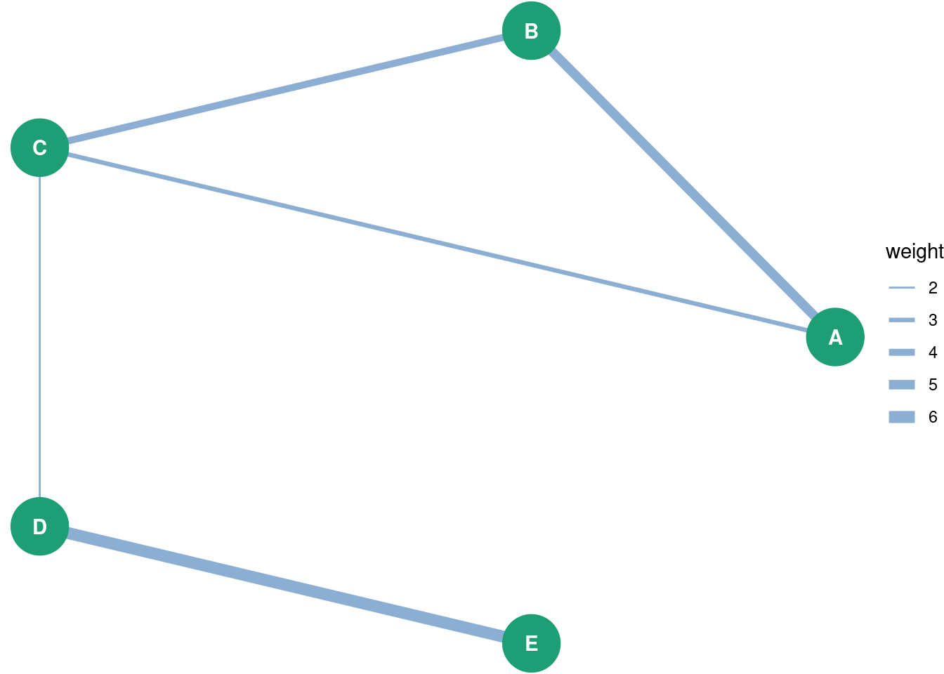
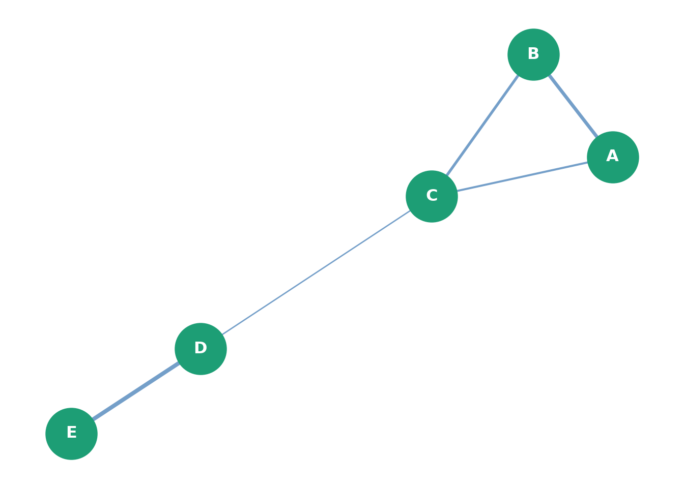
Five generic nodes (A–E) joined by five undirected weighted links. With no direction, the adjacency matrix is symmetric.

Code
library(igraph)
toy_u <- data.frame(
  from   = c("A","A","B","C","D"),
  to     = c("B","C","C","D","E"),
  weight = c(  5,   3,   4,   2,   6))
g_toy_u <- graph_from_data_frame(toy_u, directed = FALSE)
as_adjacency_matrix(g_toy_u, attr = "weight", sparse = FALSE)
  A B C D E
A 0 5 3 0 0
B 5 0 4 0 0
C 3 4 0 2 0
D 0 0 2 0 6
E 0 0 0 6 0
Code
import pandas as pd
import networkx as nx
toy_u = pd.DataFrame({
    "u"     : ["A","A","B","C","D"],
    "v"     : ["B","C","C","D","E"],
    "weight": [  5,   3,   4,   2,   6]})
G_toy_u = nx.from_pandas_edgelist(toy_u, "u", "v",
                                  edge_attr="weight",
                                  create_using=nx.Graph)
print(nx.to_pandas_adjacency(G_toy_u, weight="weight",
                             nodelist=["A","B","C","D","E"]))
     A    B    C    D    E
A  0.0  5.0  3.0  0.0  0.0
B  5.0  0.0  4.0  0.0  0.0
C  3.0  4.0  0.0  2.0  0.0
D  0.0  0.0  2.0  0.0  6.0
E  0.0  0.0  0.0  6.0  0.0

The matrix is a mirror image across the diagonal — \(A_{ij}=A_{ji}\) for every pair.

Visualizing the Undirected Network

Code
library(ggraph)
set.seed(14159)
ggraph(g_toy_u, layout = "circle") +
  geom_edge_link(aes(width = weight), alpha = 0.5, color = "#185FA5") +
  geom_node_point(size = 14, color = "#1D9E75") +
  geom_node_text(aes(label = name), color = "white", fontface = "bold") +
  scale_edge_width(range = c(0.5, 3), name = "weight") +
  theme_void()

Code
import matplotlib.pyplot as plt
pos = nx.spring_layout(G_toy_u, seed=14159)
w = [G_toy_u[u][v]["weight"] / 2 for u, v in G_toy_u.edges()]
_ = plt.figure(figsize=(7, 5))
_ = nx.draw_networkx_nodes(G_toy_u, pos, node_size=1400, node_color="#1D9E75")
_ = nx.draw_networkx_labels(G_toy_u, pos, font_color="white", font_weight="bold")
_ = nx.draw_networkx_edges(G_toy_u, pos, width=w, edge_color="#185FA5", alpha=0.6)
_ = plt.axis("off")
plt.tight_layout()
plt.show()

No arrowheads: an undirected link means the relation runs both ways by construction.

A Toy Directed Network — Edge List & Adjacency

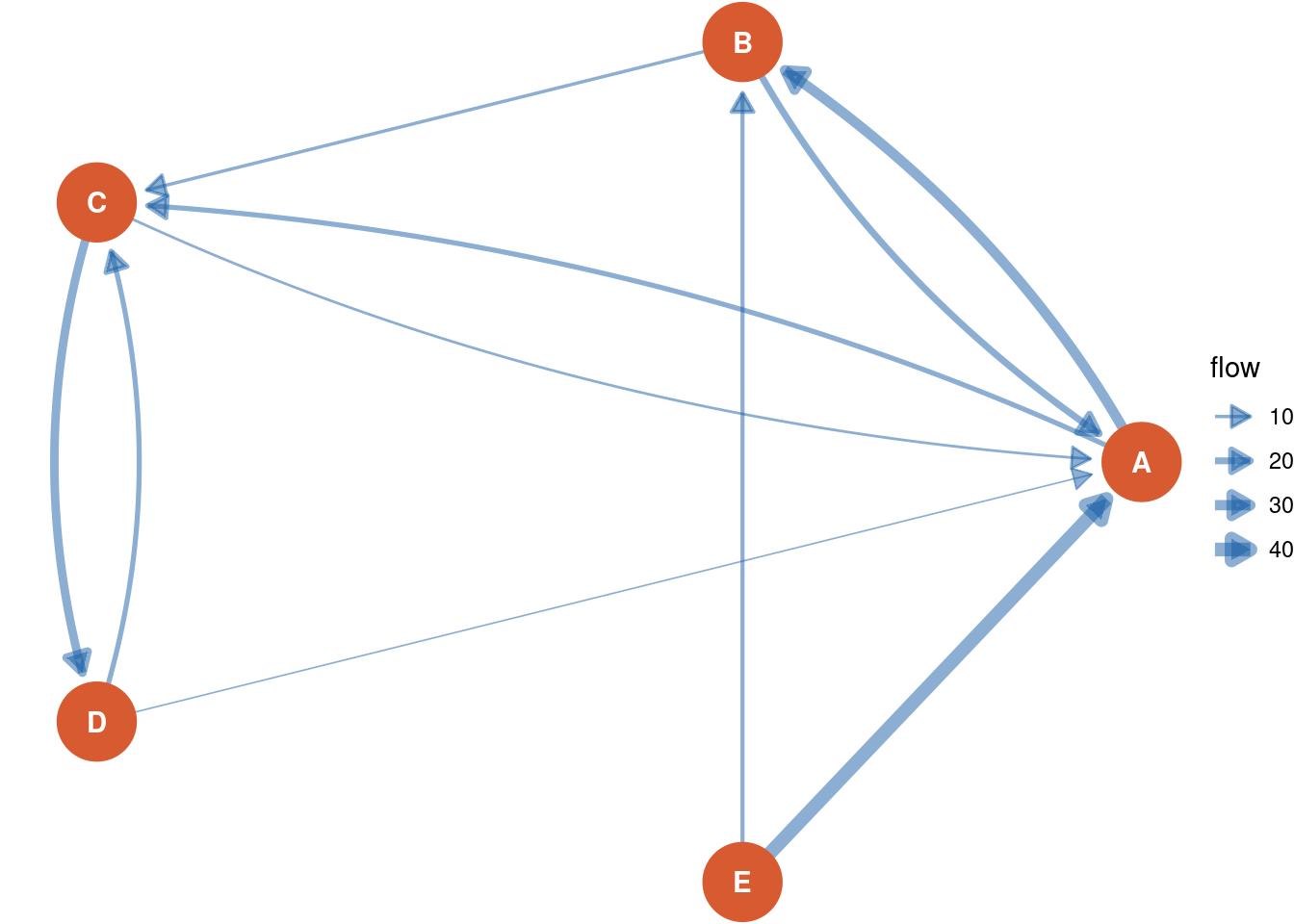
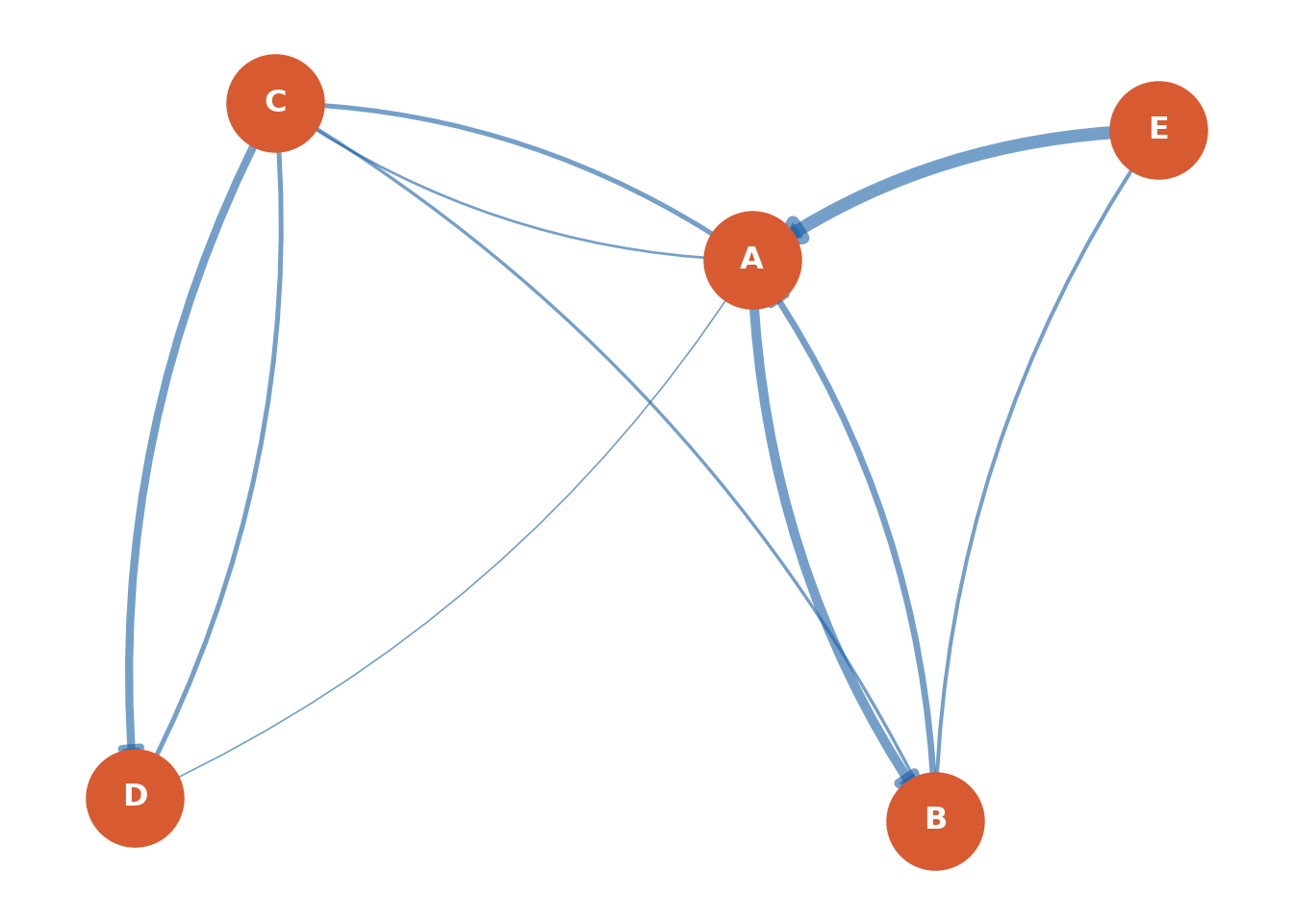
The same five generic nodes, now joined by directed links. Order matters, so \((A,B)\) and \((B,A)\) are different edges and the adjacency matrix is asymmetric.

Code
library(igraph)
toy <- data.frame(
  from   = c("A","A","B","B","C","C","D","D","E","E"),
  to     = c("B","C","A","C","A","D","C","A","A","B"),
  weight = c( 30,  15,  20,  10,   8,  25,  15,   5,  40,  12))
g_toy <- graph_from_data_frame(toy, directed = TRUE)
as_adjacency_matrix(g_toy, attr = "weight", sparse = FALSE)
   A  B  C  D E
A  0 30 15  0 0
B 20  0 10  0 0
C  8  0  0 25 0
D  5  0 15  0 0
E 40 12  0  0 0
Code
import pandas as pd
import networkx as nx
toy = pd.DataFrame({
    "from_c": ["A","A","B","B","C","C","D","D","E","E"],
    "to_c"  : ["B","C","A","C","A","D","C","A","A","B"],
    "weight": [ 30,  15,  20,  10,   8,  25,  15,   5,  40,  12]})
G_toy = nx.from_pandas_edgelist(toy, "from_c", "to_c",
                                edge_attr="weight",
                                create_using=nx.DiGraph)
print(nx.to_pandas_adjacency(G_toy, weight="weight",
                             nodelist=["A","B","C","D","E"]))
      A     B     C     D    E
A   0.0  30.0  15.0   0.0  0.0
B  20.0   0.0  10.0   0.0  0.0
C   8.0   0.0   0.0  25.0  0.0
D   5.0   0.0  15.0   0.0  0.0
E  40.0  12.0   0.0   0.0  0.0

Visualizing the Directed Network

Code
library(ggraph)
set.seed(14159)
ggraph(g_toy, layout = "circle") +
  geom_edge_fan(aes(width = weight), alpha = 0.5, color = "#185FA5",
                arrow = arrow(length = unit(3, "mm"), type = "closed"),
                end_cap = circle(7, "mm")) +
  geom_node_point(size = 14, color = "#D85A30") +
  geom_node_text(aes(label = name), color = "white", fontface = "bold") +
  scale_edge_width(range = c(0.3, 2.5), name = "flow") +
  theme_void()

Code
import matplotlib.pyplot as plt
pos = nx.spring_layout(G_toy, seed=14159)
w = [G_toy[u][v]["weight"] / 8 for u, v in G_toy.edges()]
_ = plt.figure(figsize=(7, 5))
_ = nx.draw_networkx_nodes(G_toy, pos, node_size=1400, node_color="#D85A30")
_ = nx.draw_networkx_labels(G_toy, pos, font_color="white", font_weight="bold")
_ = nx.draw_networkx_edges(G_toy, pos, width=w, edge_color="#185FA5",
                           alpha=0.6, arrowsize=18,
                           connectionstyle="arc3,rad=0.15")
_ = plt.axis("off")
plt.tight_layout()
plt.show()

Part II — Centrality: Who Matters?

Degree

Degree counts how many links a node has.

  • \(k^{\text{out}}\): number of outgoing links (out-neighbours)
  • \(k^{\text{in}}\): number of incoming links (in-neighbours)
  • In an undirected graph there is a single degree \(k_i\) — no in/out split
  • A high-degree node is a hub: connected to many others

Degree sums a row (out) or a column (in) of the adjacency matrix:

\[ k_i^{\text{out}} = \sum_{j=1}^{n} A_{ij}, \qquad k_i^{\text{in}} = \sum_{j=1}^{n} A_{ji} \]

For an undirected graph \(A=A^{\top}\), so both collapse to one number:

\[ k_i = \sum_{j=1}^{n} A_{ij} \]

Code
degree(g_toy, mode = "out")                  # number of outgoing links
degree(g_toy, mode = "in")                   # number of incoming links
degree(g_toy_u)                              # undirected: a single degree
out-degree :
A B C D E 
2 2 2 2 2 
in-degree  :
A B C D E 
4 2 3 1 0 
undirected :
A B C D E 
2 2 3 2 1 
Code
print("out-degree :", dict(G_toy.out_degree()))
out-degree : {'A': 2, 'B': 2, 'C': 2, 'D': 2, 'E': 2}
Code
print("in-degree  :", dict(G_toy.in_degree()))
in-degree  : {'A': 4, 'B': 2, 'C': 3, 'D': 1, 'E': 0}
Code
print("undirected :", dict(G_toy_u.degree()))
undirected : {'A': 2, 'B': 2, 'C': 3, 'D': 2, 'E': 1}

Strength

Strength is the weighted degree — it adds up the weights on a node’s links.

  • \(s^{\text{out}}\): total weight leaving the node; \(s^{\text{in}}\): total weight arriving
  • High strength + low degree = a few heavy links (concentrated)
  • High degree + moderate strength = many light links (diversified)
  • Undirected graph: a single strength \(s_i\)

Replace the 0/1 entries of \(A\) with the weights \(W\):

\[ s_i^{\text{out}} = \sum_{j=1}^{n} W_{ij}, \qquad s_i^{\text{in}} = \sum_{j=1}^{n} W_{ji} \]

Unweighted graph (\(W=A\)) \(\Rightarrow\) strength equals degree.

Code
strength(g_toy, mode = "out")                # total outgoing weight
strength(g_toy, mode = "in")                 # total incoming weight
strength(g_toy_u)                            # undirected: a single strength
out-strength:
 A  B  C  D  E 
45 30 33 20 52 
in-strength :
 A  B  C  D  E 
73 42 40 25  0 
undirected  :
A B C D E 
8 9 9 8 6 
Code
print("out-strength:", dict(G_toy.out_degree(weight="weight")))
out-strength: {'A': 45, 'B': 30, 'C': 33, 'D': 20, 'E': 52}
Code
print("in-strength :", dict(G_toy.in_degree(weight="weight")))
in-strength : {'A': 73, 'B': 42, 'C': 40, 'D': 25, 'E': 0}
Code
print("undirected  :", dict(G_toy_u.degree(weight="weight")))
undirected  : {'A': 8, 'B': 9, 'C': 9, 'D': 8, 'E': 6}

Closeness

Closeness measures how quickly a node can reach everyone else.

  • Small total distance to all others \(\Rightarrow\) high closeness — a node near the centre
  • Built on shortest paths: let \(d(i,j)\) be the shortest-path distance from \(i\) to \(j\)
  • Weights are costs in path algorithms! A bigger weight = a stronger tie = a shorter distance, so we pass \(1/w_{ij}\) as the edge length

\[ C_i^{\text{clo}} = \frac{n-1}{\sum_{j \neq i} d(i,j)} \]

The denominator is the total distance from \(i\) to every reachable node; dividing \(n-1\) by it puts the score on a \(0\)\(1\) scale.

Code
# invert weights: strong links = short distances
E(g_toy)$dist <- 1 / E(g_toy)$weight
round(closeness(g_toy, mode = "out", weights = E(g_toy)$dist), 2)
closeness (out):
   A    B    C    D    E 
4.84 3.45 3.09 2.07 3.26 
Code
# invert weights: strong links = short distances
for u, v in G_toy.edges():
    G_toy[u][v]["dist"] = 1 / G_toy[u][v]["weight"]
# networkx uses incoming distances, so reverse to match igraph mode="out"
clo = nx.closeness_centrality(G_toy.reverse(), distance="dist")
print("closeness:", {k: round(v, 2) for k, v in clo.items()})
closeness: {'A': 10.89, 'B': 7.76, 'C': 6.96, 'D': 4.66, 'E': 13.04}

Betweenness

Betweenness measures how often a node sits on the way between others.

  • A high-betweenness node is a broker: shortest paths funnel through it
  • High betweenness but modest degree = a structural bottleneck — remove it and paths get much longer
  • Same weight-as-distance rule applies: pass \(1/w_{ij}\) as the edge length

\[ C_i^{\text{bet}} = \sum_{s \neq i \neq t} \frac{\sigma_{st}(i)}{\sigma_{st}} \]

where \(\sigma_{st}\) is the number of shortest \(s \to t\) paths and \(\sigma_{st}(i)\) those passing through \(i\).

Code
E(g_toy)$dist <- 1 / E(g_toy)$weight
round(betweenness(g_toy, weights = E(g_toy)$dist), 2)
betweenness:
A B C D E 
5 0 5 0 0 
Code
for u, v in G_toy.edges():
    G_toy[u][v]["dist"] = 1 / G_toy[u][v]["weight"]
bet = nx.betweenness_centrality(G_toy, weight="dist")
print("betweenness:", {k: round(v, 2) for k, v in bet.items()})
betweenness: {'A': 0.42, 'B': 0.0, 'C': 0.42, 'D': 0.0, 'E': 0.0}

Small numeric differences between R and Python reflect normalization conventions, not errors.

Eigenvector, Katz–Bonacich and PageRank

It is not only how many neighbours you have — it is how important they are.

  • Eigenvector: your importance is proportional to the importance of your neighbours
  • Katz–Bonacich: sum walks of every length, discounting longer ones by \(\phi\) — the economics workhorse
  • PageRank: a random-surfer normalization built for directed graphs
  • Eigenvector centrality needs an undirected graph, so we collapse directions first

Eigenvector — importance proportional to neighbours’ importance, with \(\lambda\) the largest eigenvalue of \(A\) (Perron–Frobenius):

\[ x_i = \frac{1}{\lambda} \sum_{j} A_{ij} \, x_j \qquad \Longleftrightarrow \qquad A x = \lambda x \]

Katz–Bonacich — discounts walks by length:

\[ b = (I - \phi A)^{-1} \mathbf{1} = \sum_{k=0}^{\infty} \phi^k A^k \mathbf{1}, \qquad 0 < \phi < 1/\lambda \]

PageRank — random-surfer normalization for directed graphs:

\[ x_i = \frac{1-\alpha}{n} + \alpha \sum_{j} \frac{A_{ji}}{k_j^{\text{out}}} \, x_j, \qquad \alpha \approx 0.85 \]

Code
# eigenvector: defined for undirected graphs -> collapse directions
g_und <- as_undirected(g_toy, mode = "collapse", edge.attr.comb = "sum")
round(eigen_centrality(g_und, weights = E(g_und)$weight)$vector, 3)
# PageRank: works directly on the directed weighted graph
round(page_rank(g_toy, weights = E(g_toy)$weight)$vector, 3)
eigenvector (undirected):
    A     B     C     D     E 
1.000 0.795 0.565 0.347 0.624 
PageRank (directed):
    A     B     C     D     E 
0.263 0.185 0.299 0.222 0.030 
Code
ec = nx.eigenvector_centrality(G_toy.to_undirected(), weight="weight",
                               max_iter=1000)
pr = nx.pagerank(G_toy, weight="weight")
print("eigenvector:", {k: round(v, 3) for k, v in ec.items()})
eigenvector: {'A': 0.648, 'B': 0.419, 'C': 0.212, 'D': 0.122, 'E': 0.587}
Code
print("PageRank   :", {k: round(v, 3) for k, v in pr.items()})
PageRank   : {'A': 0.263, 'B': 0.185, 'C': 0.299, 'D': 0.222, 'E': 0.03}

Part III — Global Structure

Density, Reciprocity, Clustering

Statistics of the whole network, not a single node.

  • Density: how close the network is to complete — dense cores vs sparse peripheries
  • Reciprocity: share of links that run both ways — only meaningful for directed graphs (always \(1\) if undirected)
  • Clustering: do a node’s neighbours also link to each other? — measured by counting triangles
  • These are the summaries you compare against a null model (next slides)

Density — share of possible edges that exist:

\[ \rho = \frac{L}{n(n-1)}, \qquad L = |E| \]

Reciprocity — share of edges that run both ways:

\[ r = \frac{L^{\leftrightarrow}}{L}, \qquad L^{\leftrightarrow} = \#\{(i,j) \in E : (j,i) \in E\} \]

Clustering (transitivity) — are a node’s neighbours linked to each other?

\[ C = \frac{3 \times \#\text{triangles}}{\#\text{connected triples}} \]

Code
edge_density(g_toy)               # rho
reciprocity(g_toy)                # r
transitivity(g_toy)               # C  (directions ignored)
mean_distance(g_toy)              # average shortest path length
density      : 0.5 
reciprocity  : 0.6 
transitivity : 0.686 
mean distance: 24.062 
Code
print("density      :", round(nx.density(G_toy), 3))
density      : 0.5
Code
print("reciprocity  :", round(nx.reciprocity(G_toy), 3))
reciprocity  : 0.6
Code
print("transitivity :", round(nx.transitivity(nx.Graph(G_toy)), 3))
transitivity : 0.643
Code
# average over reachable ordered pairs (matches igraph mean_distance)
dists = [d for src, tgt in nx.all_pairs_shortest_path_length(G_toy)
         for node, d in tgt.items() if d > 0]
print("mean distance:", round(sum(dists) / len(dists), 3))
mean distance: 1.438

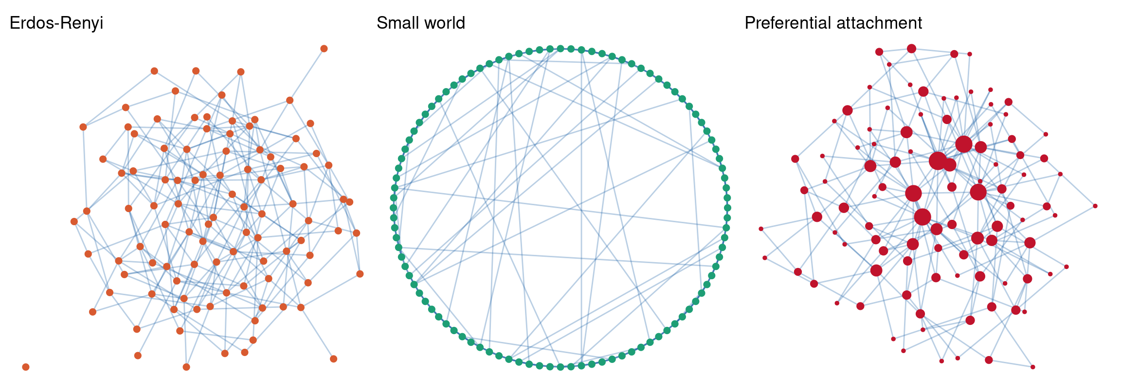
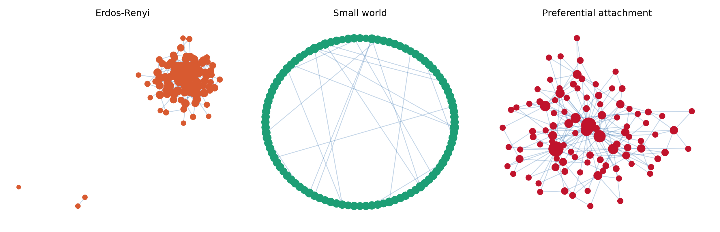
Degree Distributions and Random Graph Benchmarks

To say a network is “surprisingly clustered” you need a null model. Three classics:

  • Erdős–Rényi \(G(n,p)\): every edge appears independently — the “pure chance” benchmark
  • Watts–Strogatz: a ring lattice with a little rewiring — high clustering and short paths (small world)
  • Barabási–Albert: new nodes attach to popular ones — generates hubs and a fat-tailed degree distribution
  • Fat tails mean a few very connected nodes carry most of the structure

Erdős–Rényi — Poisson-like degree distribution:

\[ P(k) = \binom{n-1}{k} p^k (1-p)^{n-1-k} \approx \frac{e^{-\bar{k}} \, \bar{k}^k}{k!} \]

Watts–Strogatz — a ring lattice rewired with probability \(\beta\) (no closed-form \(P(k)\); described by high clustering with short path length).

Barabási–Albert — scale-free power-law tail:

\[ P(k) \sim k^{-\gamma}, \qquad \gamma \approx 3 \]

Code
set.seed(14159)
g_er <- sample_gnp(100, p = 0.05)                 # Erdos-Renyi
g_ws <- sample_smallworld(1, 100, nei = 3, p = 0.05)  # Watts-Strogatz
g_ba <- sample_pa(100, m = 2, directed = FALSE)   # Barabasi-Albert
p1 <- ggraph(g_er, layout = "stress") +
  geom_edge_link(alpha = .3, color = "#185FA5") +
  geom_node_point(color = "#D85A30", size = 2) +
  labs(title = "Erdos-Renyi") + theme_void()
p2 <- ggraph(g_ws, layout = "circle") +
  geom_edge_link(alpha = .3, color = "#185FA5") +
  geom_node_point(color = "#1D9E75", size = 2) +
  labs(title = "Small world") + theme_void()
p3 <- ggraph(g_ba, layout = "stress") +
  geom_edge_link(alpha = .3, color = "#185FA5") +
  geom_node_point(aes(size = degree(g_ba)), color = "#C0132C",
                  show.legend = FALSE) +
  labs(title = "Preferential attachment") + theme_void()
p1 + p2 + p3

Code
import numpy as np
G_er = nx.erdos_renyi_graph(100, 0.05, seed=14159)
G_ws = nx.watts_strogatz_graph(100, 6, 0.05, seed=14159)
G_ba = nx.barabasi_albert_graph(100, 2, seed=14159)
fig, axes = plt.subplots(1, 3, figsize=(13, 4.2))
for G, ax, ttl, col in [(G_er, axes[0], "Erdos-Renyi", "#D85A30"),
                        (G_ws, axes[1], "Small world", "#1D9E75"),
                        (G_ba, axes[2], "Preferential attachment", "#C0132C")]:
    pos = (nx.circular_layout(G) if ttl == "Small world"
           else nx.spring_layout(G, seed=14159))
    deg = dict(G.degree())
    _ = nx.draw_networkx_nodes(G, pos, ax=ax, node_color=col,
                               node_size=[25 + 12 * deg[v] for v in G])
    _ = nx.draw_networkx_edges(G, pos, ax=ax, alpha=0.25,
                               edge_color="#185FA5")
    ax.set_title(ttl); ax.axis("off")
plt.tight_layout()
plt.show()

Community Detection — Modularity

A community is a group of nodes more densely connected internally than externally.

  • Modularity \(Q\) compares observed within-group weight to what a random rewiring with the same strengths would give
  • The Louvain algorithm greedily maximizes \(Q\) — fast, standard, works on weighted graphs
  • Defined for undirected graphs, so we collapse directions first
  • Rule of thumb: \(Q > 0.3\) indicates meaningful community structure

Modularity of a partition \(\{c_i\}\) (Newman), with \(s_i\) the node strengths:

\[ Q = \frac{1}{2m} \sum_{i,j} \left( W_{ij} - \frac{s_i \, s_j}{2m} \right) \delta(c_i, c_j), \qquad m = \tfrac{1}{2}\sum_{i,j} W_{ij} \]

\(\delta(c_i,c_j)=1\) when \(i\) and \(j\) share a community, else \(0\). Louvain searches partitions to make \(Q\) as large as possible.

Code
# modularity is undirected -> collapse directions, summing weights
g_und <- as_undirected(g_toy, mode = "collapse", edge.attr.comb = "sum")
set.seed(14159)
cl <- cluster_louvain(g_und, weights = E(g_und)$weight)
membership(cl)      # community label per node
modularity(cl)      # Q of the partition
membership:
A B C D E 
1 1 2 2 1 
modularity Q: 0.23 
Code
Gu = G_toy.to_undirected()
comms = nx.community.louvain_communities(Gu, weight="weight", seed=14159)
Q = nx.community.modularity(Gu, comms, weight="weight")
print("communities:", [sorted(c) for c in comms])
print("modularity Q:", round(Q, 3))

Comparing Network Structures

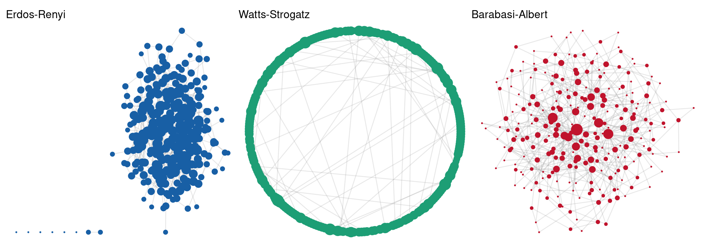
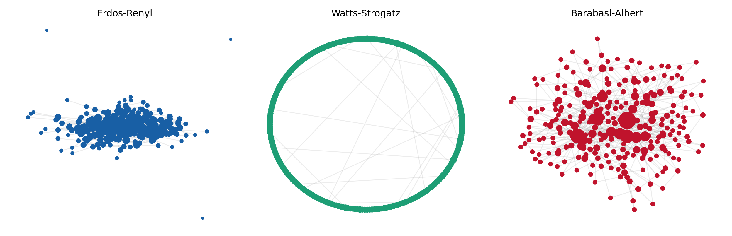
Three Networks, Same Size

We fix the size (\(n=250\) nodes) and the mean degree (\(\bar{k}\approx 4\)), then change only the wiring rule. Any difference in clustering, path length or degree spread is therefore due to structure alone.

  • Erdős–Rényi \(G(n,p)\): connect every pair with the same probability — pure chance
  • Watts–Strogatz: a ring lattice with a few links rewired — a small world
  • Barabási–Albert: new nodes attach to already-popular ones — grows hubs
  • Sources: Erdős & Rényi (1960); Watts & Strogatz (1998, doi:10.1038/30918); Barabási & Albert (1999, doi:10.1126/science.286.5439.509)
Code
library(ggraph); library(patchwork)
set.seed(14159)
n <- 250
c_er <- sample_gnp(n, p = 4 / (n - 1))              # Erdos-Renyi
c_ws <- sample_smallworld(1, n, nei = 2, p = 0.05)  # Watts-Strogatz
c_ba <- sample_pa(n, m = 2, directed = FALSE)       # Barabasi-Albert
# one small helper: node size shows degree, so hubs pop out
plot_net <- function(g, ttl, col, lay = "stress") {
  ggraph(g, layout = lay) +
    geom_edge_link(alpha = 0.2, color = "grey55") +
    geom_node_point(aes(size = degree(g)), color = col, show.legend = FALSE) +
    scale_size(range = c(0.4, 6)) +
    labs(title = ttl) + theme_void()
}
plot_net(c_er, "Erdos-Renyi", "#185FA5") +
  plot_net(c_ws, "Watts-Strogatz", "#1D9E75", "circle") +
  plot_net(c_ba, "Barabasi-Albert", "#C0132C")

Code
import numpy as np, matplotlib.pyplot as plt
n = 250
cg_er = nx.gnp_random_graph(n, 4 / (n - 1), seed=14159)
cg_ws = nx.watts_strogatz_graph(n, 4, 0.05, seed=14159)
cg_ba = nx.barabasi_albert_graph(n, 2, seed=14159)
fig, axes = plt.subplots(1, 3, figsize=(13, 4.2))
specs = [(cg_er, axes[0], "Erdos-Renyi", "#185FA5"),
         (cg_ws, axes[1], "Watts-Strogatz", "#1D9E75"),
         (cg_ba, axes[2], "Barabasi-Albert", "#C0132C")]
for G, ax, ttl, col in specs:
    pos = (nx.circular_layout(G) if ttl == "Watts-Strogatz"
           else nx.spring_layout(G, seed=14159))
    deg = dict(G.degree())
    _ = nx.draw_networkx_nodes(G, pos, ax=ax, node_color=col,
                               node_size=[8 + 9 * deg[v] for v in G])
    _ = nx.draw_networkx_edges(G, pos, ax=ax, alpha=0.15, edge_color="grey")
    ax.set_title(ttl); ax.axis("off")
plt.tight_layout()
plt.show()

Same number of nodes and links in all three — yet the pictures could hardly look more different.

Structural Fingerprints

Model Edges Mean degree Clustering Mean distance Diameter Assortativity Max degree
Erdős–Rényi 491 3.93 0.014 4.08 8 0.063 10
Watts–Strogatz 500 4.00 0.351 6.50 13 -0.083 6
Barabási–Albert 497 3.98 0.026 3.62 7 -0.063 35

WS clustering is ~10× the others; BA max degree is a huge hub (mean is only 4) and its paths are the shortest.

Code
measure <- function(g) data.frame(
  edges     = ecount(g),
  mean_deg  = round(mean(degree(g)), 2),
  cluster   = round(transitivity(g), 3),
  mean_dist = round(mean_distance(g), 2),
  diameter  = diameter(g),
  assort    = round(assortativity_degree(g), 3),
  max_deg   = max(degree(g)))
rbind(ER = measure(c_er), WS = measure(c_ws), BA = measure(c_ba))
   edges mean_deg cluster mean_dist diameter assort max_deg
ER   491     3.93   0.014      4.08        8  0.063      10
WS   500     4.00   0.351      6.50       13 -0.083       6
BA   497     3.98   0.026      3.62        7 -0.063      35
Code
import pandas as pd
def mean_dist(G):                    # average over reachable pairs
    ds = [d for _, tgt in nx.all_pairs_shortest_path_length(G)
          for _, d in tgt.items() if d > 0]
    return round(sum(ds) / len(ds), 2)
def giant_diameter(G):               # diameter of the largest component
    C = max(nx.connected_components(G), key=len)
    return nx.diameter(G.subgraph(C))
def measure(G):
    deg = [d for _, d in G.degree()]
    return dict(edges=G.number_of_edges(), mean_deg=round(np.mean(deg), 2),
        cluster=round(nx.transitivity(G), 3), mean_dist=mean_dist(G),
        diameter=giant_diameter(G),
        assort=round(nx.degree_assortativity_coefficient(G), 3),
        max_deg=max(deg))
tab = pd.DataFrame([measure(cg_er), measure(cg_ws), measure(cg_ba)],
                   index=["ER", "WS", "BA"])
print(tab.to_string())

Degree Distributions Compared

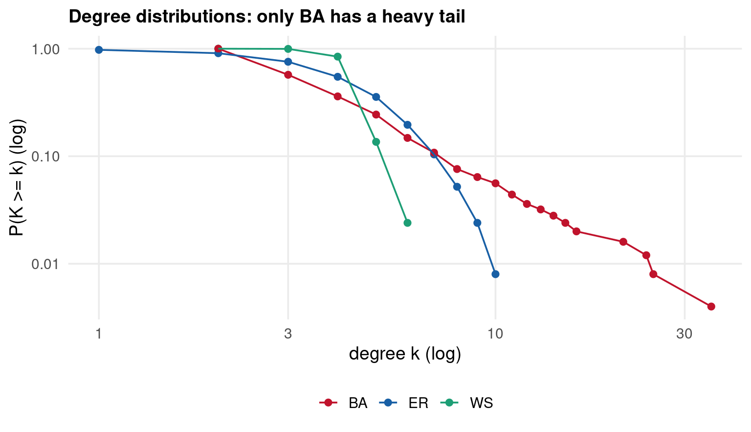
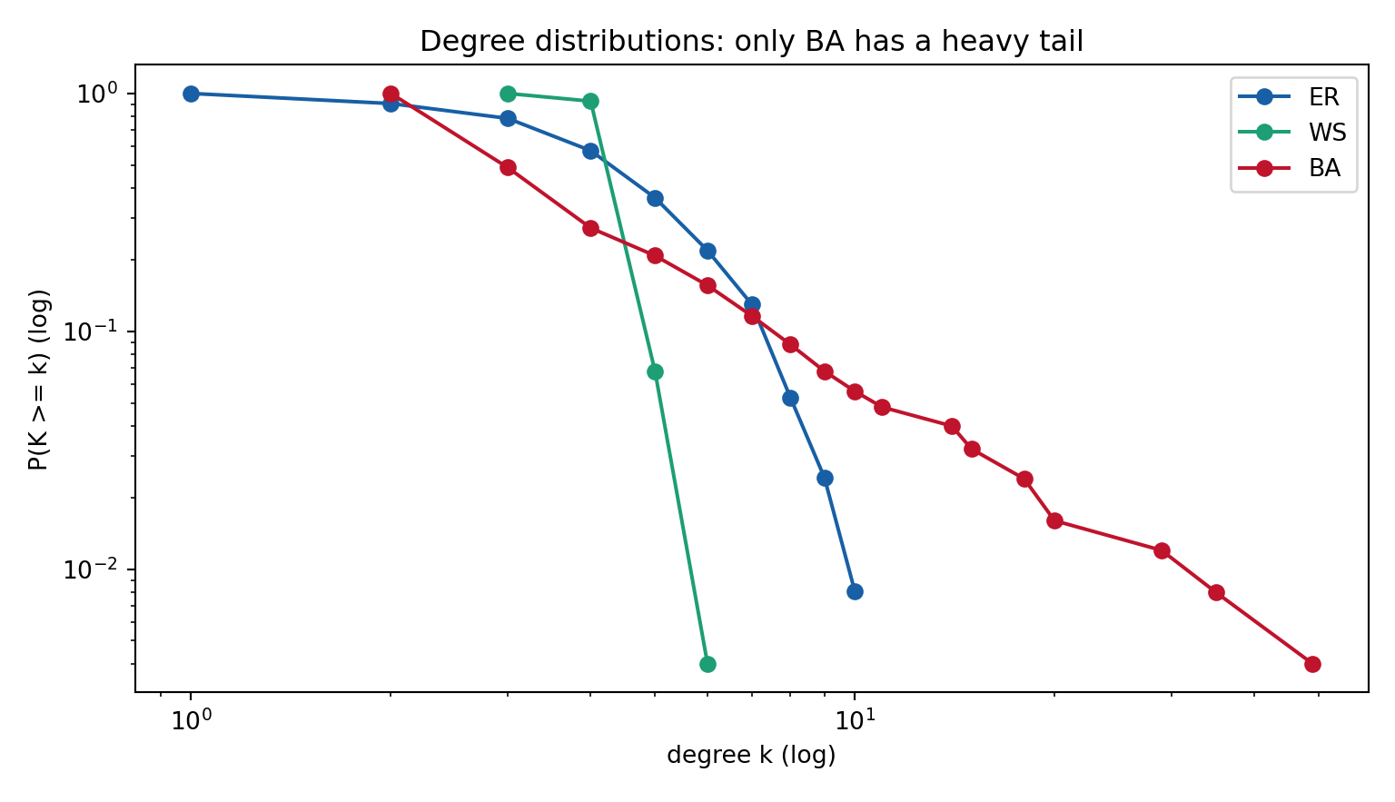
The degree distribution is the clearest fingerprint. On a log-log plot of the tail (complementary CDF, \(P(K \ge k)\)):

  • ER: a Poisson bump — degrees cluster tightly around the mean, the curve falls off fast
  • WS: even narrower — almost every node has the same degree
  • BA: a straight line = a power-law tail — a handful of nodes have enormous degree
Code
# complementary CDF of the degree sequence: P(K >= k)
ccdf_df <- function(g, label) {
  d  <- degree(g)
  ks <- sort(unique(d[d > 0]))
  cc <- numeric(length(ks))
  for (i in seq_along(ks)) cc[i] <- mean(d >= ks[i])
  data.frame(k = ks, ccdf = cc, model = label)
}
df <- rbind(ccdf_df(c_er, "ER"), ccdf_df(c_ws, "WS"), ccdf_df(c_ba, "BA"))
ggplot(df, aes(k, ccdf, color = model)) +
  geom_point(size = 2) + geom_line() +
  scale_x_log10() + scale_y_log10() +
  scale_color_manual(values = c(ER = "#185FA5", WS = "#1D9E75", BA = "#C0132C")) +
  labs(x = "degree k (log)", y = "P(K >= k) (log)", color = NULL,
       title = "Degree distributions: only BA has a heavy tail")

Code
def ccdf(G):
    d  = np.array([x for _, x in G.degree() if x > 0])
    ks = np.sort(np.unique(d))
    cc = np.array([np.mean(d >= k) for k in ks])
    return ks, cc
_ = plt.figure(figsize=(8, 4.6))
for G, lab, col in [(cg_er, "ER", "#185FA5"),
                    (cg_ws, "WS", "#1D9E75"),
                    (cg_ba, "BA", "#C0132C")]:
    ks, cc = ccdf(G)
    _ = plt.loglog(ks, cc, "o-", color=col, label=lab)
_ = plt.xlabel("degree k (log)"); _ = plt.ylabel("P(K >= k) (log)")
_ = plt.title("Degree distributions: only BA has a heavy tail")
_ = plt.legend(); plt.tight_layout(); plt.show()

What the Numbers Say

Three wiring rules, three very different worlds:

  • Erdős–Rényi — low clustering, short paths, Poisson degrees, assortativity \(\approx 0\). The null model: what “no structure” looks like.
  • Watts–Strogatzhigh clustering and short paths at the same time: the small-world property of social and collaboration networks.
  • Barabási–Albert — a fat-tailed degree distribution: a few dominant hubs, the shortest paths of all, and negative assortativity (hubs attach to the periphery).

Why economists care: real trade and production networks are hub-dominated, closer to BA than to ER. That is exactly why idiosyncratic shocks to central sectors/countries do not wash out but drive aggregate volatility — Acemoglu, Carvalho, Ozdaglar & Tahbaz-Salehi (2012, doi:10.3982/ECTA9623). Small-world structure, in turn, governs how fast shocks and information diffuse.

Further reading: Newman, Networks: An Introduction (2010, doi:10.1093/oso/9780198805090.001.0001); Jackson, Social and Economic Networks (2008, Princeton UP, JSTOR). Numbers differ slightly between R (igraph) and Python (networkx) because the two libraries use different random generators — the qualitative fingerprints are identical.

Part IV — Application: The EU Trade Network

Data — Eurostat Table ext_tec03

Annual international trade of EU countries by partner country (Trade by Enterprise Characteristics). We use total exports in thousands of euros, 2012–2024.

You could download it live (as the original lab notebook did):

library(eurostat)
ext_tec03 <- get_eurostat(id = "ext_tec03",
                          stringsAsFactors = FALSE,
                          time_format = "num")

In class we use the snapshot already saved at ../data/ext_tec03.csv:

Code
trade <- read.csv("../data/ext_tec03.csv")
str(trade)
'data.frame':   616744 obs. of  8 variables:
 $ freq    : chr  "A" "A" "A" "A" ...
 $ unit    : chr  "NR_ENT" "NR_ENT" "NR_ENT" "NR_ENT" ...
 $ stk_flow: chr  "EXP" "EXP" "EXP" "EXP" ...
 $ nace_r2 : chr  "A_F_H-U" "A_F_H-U" "A_F_H-U" "A_F_H-U" ...
 $ partner : chr  "AE" "AE" "AE" "AE" ...
 $ geo     : chr  "AT" "AT" "AT" "AT" ...
 $ time    : int  2012 2013 2014 2015 2016 2017 2018 2019 2020 2021 ...
 $ values  : num  119 117 130 151 133 123 109 123 139 184 ...
Code
trade = pd.read_csv("../data/ext_tec03.csv")
print(trade.head())
print(trade.shape)

Dimensions: freq, unit (THS_EUR = thousand €, NR_ENT = number of enterprises), stk_flow (EXP/IMP), nace_r2 (sector), partner, geo (reporter), time, values.

Building the Edge List

We keep: exports, total economy, thousand euros, EU-27 reporters and partners — one directed weighted edge per country pair. Weights are converted to shares of the exporter’s world exports so that small and large countries are comparable.

\[ w_{ij} = 100 \times \frac{\text{EXP}_{i \to j}}{\text{EXP}_{i \to \text{WORLD}}} \]

Code
eu27 <- c("AT","BE","BG","CY","CZ","DE","DK","EE","EL","ES","FI","FR",
          "HR","HU","IE","IT","LT","LU","LV","MT","NL","PL","PT","RO",
          "SE","SI","SK")
exp_tot <- trade %>%
  filter(unit == "THS_EUR", stk_flow == "EXP", nace_r2 == "TOTAL")
world <- exp_tot %>%
  filter(geo %in% eu27, partner == "WORLD") %>%
  select(geo, time, world = values)
edges_all <- exp_tot %>%
  filter(geo %in% eu27, partner %in% eu27,
         geo != partner, !is.na(values)) %>%
  inner_join(world, by = c("geo", "time")) %>%
  mutate(share = round(100 * values / world, 2)) %>%
  select(time, from = geo, to = partner, value = values, share)
write.csv(edges_all, "../data/trade_edges.csv", row.names = FALSE)
head(edges_all)
rows: 8862  years: 2012-2024 
  time from to   value share
1 2012   BE AT 3209881  0.94
2 2013   BE AT 3363683  0.97
3 2014   BE AT 3607532  1.04
4 2015   BE AT 3549116  1.01
5 2016   BE AT 3556102  1.01
6 2017   BE AT 3814261  1.03
Code
eu27 = ["AT","BE","BG","CY","CZ","DE","DK","EE","EL","ES","FI","FR",
        "HR","HU","IE","IT","LT","LU","LV","MT","NL","PL","PT","RO",
        "SE","SI","SK"]
exp_tot = trade[(trade.unit == "THS_EUR") & (trade.stk_flow == "EXP")
                & (trade.nace_r2 == "TOTAL")]
world = (exp_tot[(exp_tot.geo.isin(eu27)) & (exp_tot.partner == "WORLD")]
         [["geo", "time", "values"]].rename(columns={"values": "world"}))
edges = exp_tot[(exp_tot.geo.isin(eu27)) & (exp_tot.partner.isin(eu27))
                & (exp_tot.geo != exp_tot.partner)].dropna(subset=["values"])
edges = edges.merge(world, on=["geo", "time"])
edges["share"] = round(100 * edges["values"] / edges["world"], 2)
edges = edges.rename(columns={"geo": "from_c", "partner": "to_c"})
print(edges[["time", "from_c", "to_c", "values", "share"]].head())
print("rows:", len(edges))

Intra-EU Export Shares

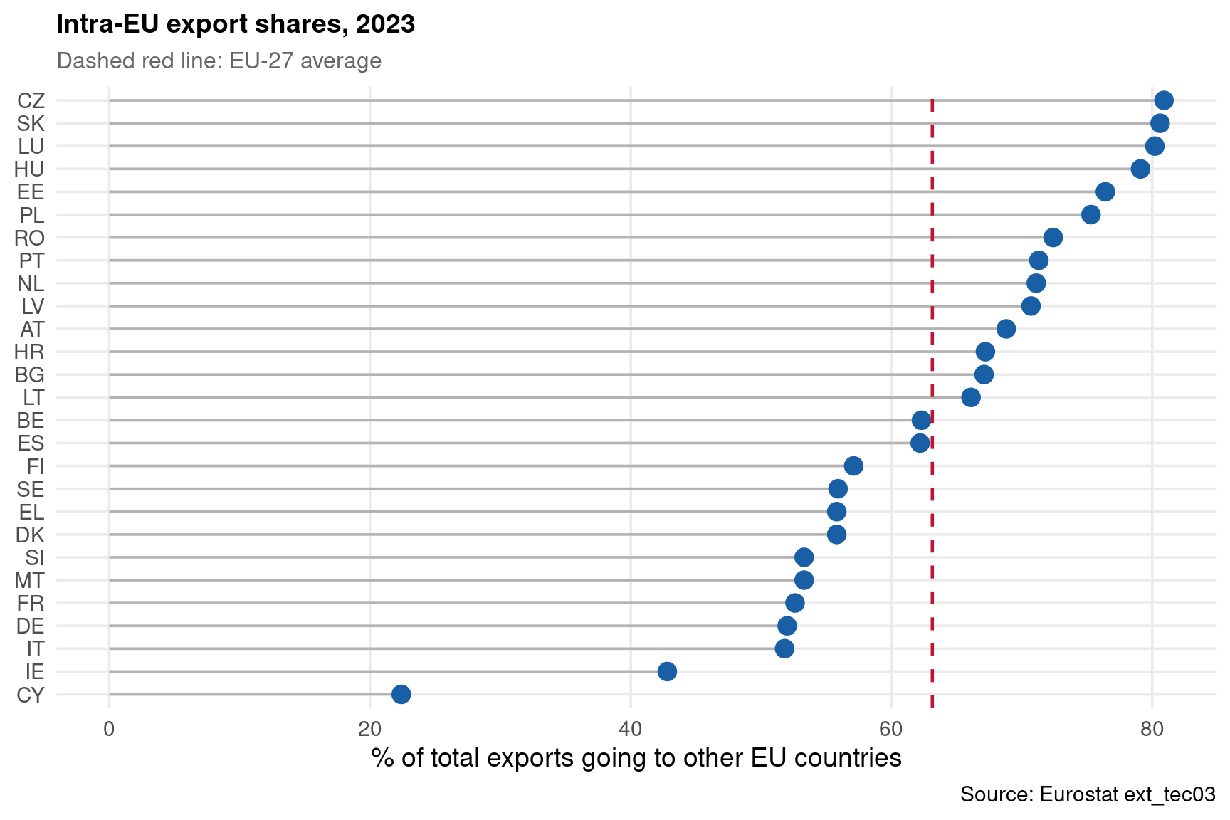
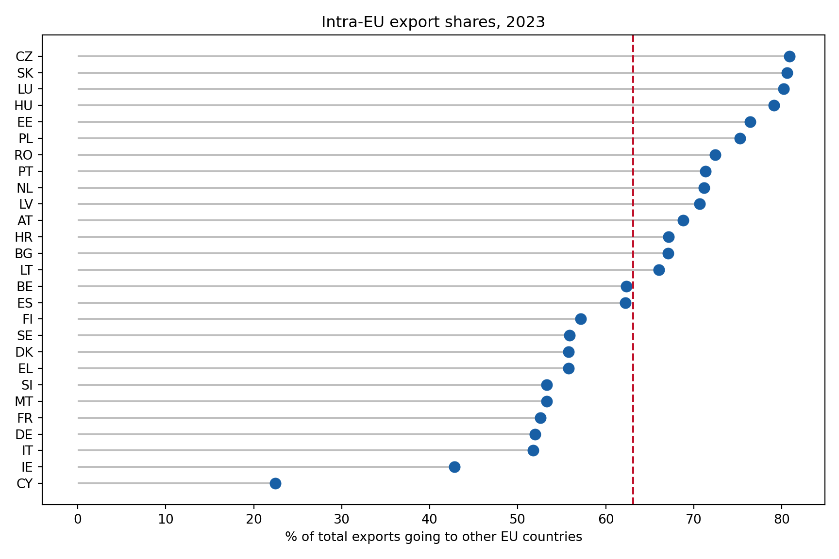
How dependent is each member state on the single market? (Update of the lab’s 2017 chart to 2023.)

Code
intra <- trade %>%
  filter(unit == "THS_EUR", stk_flow == "EXP", nace_r2 == "TOTAL",
         time == 2023, geo %in% eu27,
         partner %in% c("INT_EU", "WORLD")) %>%
  pivot_wider(id_cols = geo, names_from = partner, values_from = values) %>%
  mutate(perc = round(100 * INT_EU / WORLD, 1))
ggplot(intra, aes(x = reorder(geo, perc), y = perc)) +
  geom_segment(aes(xend = reorder(geo, perc), y = 0, yend = perc),
               color = "grey70") +
  geom_point(size = 4, color = "#185FA5") +
  geom_hline(yintercept = mean(intra$perc), linetype = "dashed",
             color = "#C0132C", linewidth = 0.8) +
  coord_flip() +
  labs(x = NULL, y = "% of total exports going to other EU countries",
       title = "Intra-EU export shares, 2023",
       subtitle = "Dashed red line: EU-27 average",
       caption = "Source: Eurostat ext_tec03")

Code
sub = trade[(trade.unit == "THS_EUR") & (trade.stk_flow == "EXP")
            & (trade.nace_r2 == "TOTAL") & (trade.time == 2023)
            & (trade.geo.isin(eu27))
            & (trade.partner.isin(["INT_EU", "WORLD"]))]
piv = sub.pivot_table(index="geo", columns="partner", values="values")
piv["perc"] = 100 * piv["INT_EU"] / piv["WORLD"]
piv = piv.sort_values("perc")
_ = plt.figure(figsize=(9, 6))
_ = plt.hlines(piv.index, 0, piv["perc"], color="grey", alpha=0.5)
_ = plt.plot(piv["perc"], piv.index, "o", color="#185FA5", markersize=8)
_ = plt.axvline(piv["perc"].mean(), color="#C0132C", linestyle="--")
_ = plt.xlabel("% of total exports going to other EU countries")
_ = plt.title("Intra-EU export shares, 2023")
plt.tight_layout()
plt.show()

Constructing the Trade Network

An edge \(i \to j\) enters the graph when \(j\) absorbs more than 5% of \(i\)’s world exports — we keep only economically meaningful dependencies.

Code
strong <- edges_all %>% filter(time == 2023, share > 5)
g_eu <- graph_from_data_frame(strong %>% select(from, to),
                              directed = TRUE)
E(g_eu)$share <- strong$share
g_eu
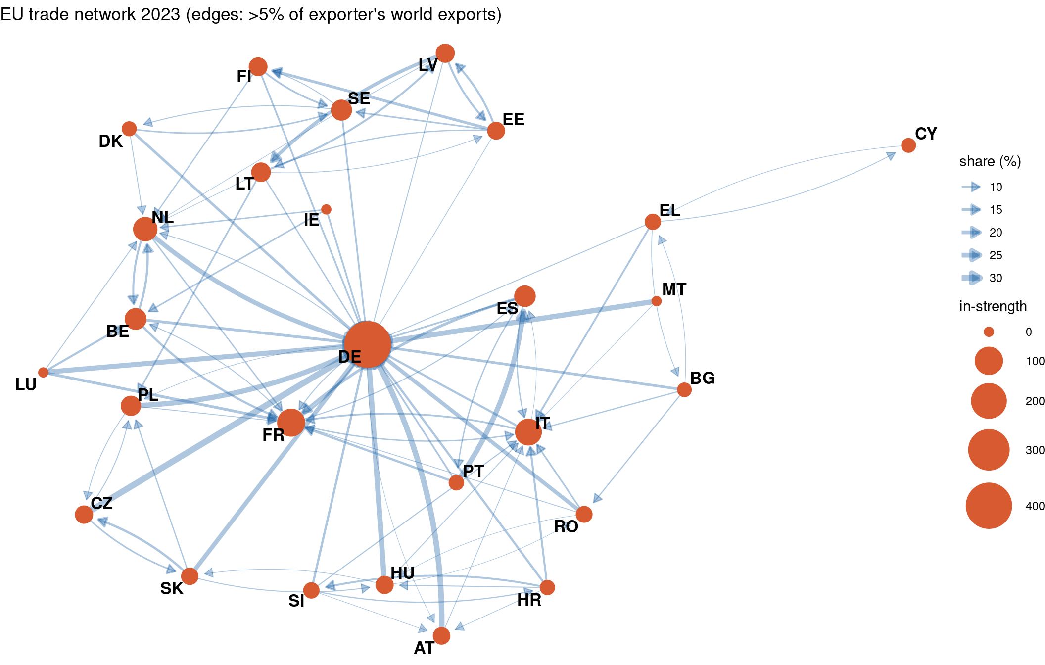
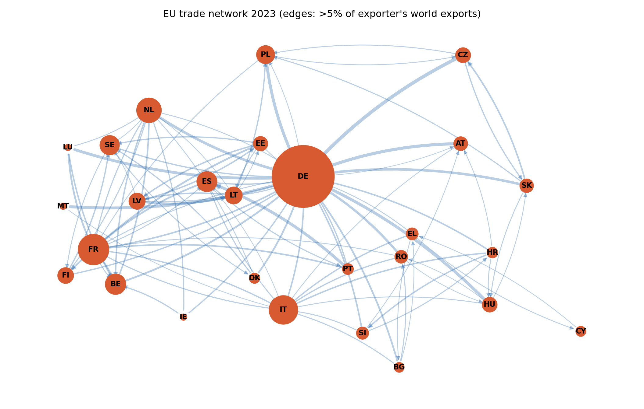
nodes: 27   edges: 95 
density     : 0.135 
reciprocity : 0.463 
transitivity: 0.358 
mean distance: 2.433 
Code
strong = edges[(edges.time == 2023) & (edges.share > 5)]
G_eu = nx.from_pandas_edgelist(strong, "from_c", "to_c",
                               edge_attr="share",
                               create_using=nx.DiGraph)
print("nodes:", G_eu.number_of_nodes(),
      " edges:", G_eu.number_of_edges())
print("density    :", round(nx.density(G_eu), 3))
print("reciprocity:", round(nx.reciprocity(G_eu), 3))
print("transitivity:", round(nx.transitivity(nx.Graph(G_eu)), 3))

Visualizing the EU Trade Network

Code
V(g_eu)$instr <- strength(g_eu, mode = "in", weights = E(g_eu)$share)
set.seed(14159)
ggraph(g_eu, layout = "stress") +
  geom_edge_fan(aes(width = share), alpha = 0.35, color = "#185FA5",
                arrow = arrow(length = unit(2.5, "mm"), type = "closed"),
                end_cap = circle(4, "mm")) +
  geom_node_point(aes(size = instr), color = "#D85A30") +
  geom_node_text(aes(label = name), repel = TRUE, fontface = "bold",
                 size = 4.5) +
  scale_edge_width(range = c(0.2, 2.2), name = "share (%)") +
  scale_size(range = c(3, 16), name = "in-strength") +
  labs(title = "EU trade network 2023 (edges: >5% of exporter's world exports)") +
  theme_void()

Code
instr = dict(G_eu.in_degree(weight="share"))
pos = nx.spring_layout(G_eu, seed=14159, k=1.2)
_ = plt.figure(figsize=(11, 7))
_ = nx.draw_networkx_nodes(G_eu, pos,
    node_size=[60 + 14 * instr[v] for v in G_eu],
    node_color="#D85A30")
_ = nx.draw_networkx_edges(G_eu, pos, alpha=0.3, edge_color="#185FA5",
    width=[0.2 + G_eu[u][v]["share"] / 8 for u, v in G_eu.edges()],
    arrowsize=10, connectionstyle="arc3,rad=0.1")
_ = nx.draw_networkx_labels(G_eu, pos, font_size=9, font_weight="bold")
_ = plt.title("EU trade network 2023 (edges: >5% of exporter's world exports)")
_ = plt.axis("off")
plt.tight_layout()
plt.show()

Centrality — Who Is the Hub of EU Trade?

Code
E(g_eu)$dist <- 1 / E(g_eu)$share
centr <- data.frame(
  country  = V(g_eu)$name,
  in_deg   = degree(g_eu, mode = "in"),
  in_str   = round(strength(g_eu, mode = "in",  weights = E(g_eu)$share), 1),
  betw     = round(betweenness(g_eu, weights = E(g_eu)$dist), 1),
  pagerank = round(page_rank(g_eu, weights = E(g_eu)$share)$vector, 3))
centr[order(-centr$pagerank), ][1:10, ]
 country in_deg in_str betw pagerank
      DE     25  412.4  157    0.281
      FR      9   96.6   54    0.156
      NL      8   61.0   25    0.095
      PL      4   30.8   79    0.065
      IT     10   83.9   15    0.065
      AT      3   16.2    0    0.057
      BE      4   41.0    5    0.055
      ES      3   38.9   26    0.049
      CZ      2   19.7   56    0.016
      PT      1    8.5    0    0.014
Code
for u, v in G_eu.edges():
    G_eu[u][v]["dist"] = 1 / G_eu[u][v]["share"]
cen = pd.DataFrame({
    "in_deg":   dict(G_eu.in_degree()),
    "in_str":   dict(G_eu.in_degree(weight="share")),
    "betw":     nx.betweenness_centrality(G_eu, weight="dist"),
    "pagerank": nx.pagerank(G_eu, weight="share")})
print(cen.sort_values("pagerank", ascending=False).round(3).head(10))
    in_deg  in_str   betw  pagerank
DE      25  412.36  0.242     0.281
FR       9   96.57  0.083     0.156
NL       8   60.98  0.038     0.095
IT      10   83.93  0.023     0.065
PL       4   30.78  0.122     0.065
AT       3   16.25  0.000     0.057
BE       4   40.98  0.008     0.055
ES       3   38.94  0.040     0.049
CZ       2   19.69  0.086     0.016
PT       1    8.51  0.000     0.014

Germany is the hub on every measure — 25 of 26 partners send it more than 5% of their exports. France, the Netherlands, Italy and Poland form a second tier; Poland’s high betweenness reflects its gateway role for the Baltics and Central Europe.

Results Table

EU trade network 2023 — top 10 by PageRank
Country In-degree In-strength Betweenness PageRank
DE 25 412.4 157 0.281
FR 9 96.6 54 0.156
NL 8 61.0 25 0.095
PL 4 30.8 79 0.065
IT 10 83.9 15 0.065
AT 3 16.2 0 0.057
BE 4 41.0 5 0.055
ES 3 38.9 26 0.049
CZ 2 19.7 56 0.016
PT 1 8.5 0 0.014
\begin{table}

\caption{\label{tab:results-latex}EU trade network 2023 --- top 10 by PageRank}
\centering
\begin{tabular}[t]{lrrrr}
\toprule
Country & In-degree & In-strength & Betweenness & PageRank\\
\midrule
DE & 25 & 412.4 & 157 & 0.281\\
FR & 9 & 96.6 & 54 & 0.156\\
NL & 8 & 61.0 & 25 & 0.095\\
PL & 4 & 30.8 & 79 & 0.065\\
IT & 10 & 83.9 & 15 & 0.065\\
\addlinespace
AT & 3 & 16.2 & 0 & 0.057\\
BE & 4 & 41.0 & 5 & 0.055\\
ES & 3 & 38.9 & 26 & 0.049\\
CZ & 2 & 19.7 & 56 & 0.016\\
PT & 1 & 8.5 & 0 & 0.014\\
\bottomrule
\end{tabular}
\end{table}
Code
tab10 <- centr[order(-centr$pagerank), ][1:10, ]
kbl(tab10, row.names = FALSE,
    col.names = c("Country", "In-degree", "In-strength",
                  "Betweenness", "PageRank")) |>
  kable_styling(font_size = 24, full_width = FALSE)
 country in_deg in_str betw pagerank
      DE     25  412.4  157    0.281
      FR      9   96.6   54    0.156
      NL      8   61.0   25    0.095
      PL      4   30.8   79    0.065
      IT     10   83.9   15    0.065
      AT      3   16.2    0    0.057
      BE      4   41.0    5    0.055
      ES      3   38.9   26    0.049
      CZ      2   19.7   56    0.016
      PT      1    8.5    0    0.014
Code
top10 = cen.sort_values("pagerank", ascending=False).head(10).round(3)
print(top10.to_string())
    in_deg  in_str   betw  pagerank
DE      25  412.36  0.242     0.281
FR       9   96.57  0.083     0.156
NL       8   60.98  0.038     0.095
IT      10   83.93  0.023     0.065
PL       4   30.78  0.122     0.065
AT       3   16.25  0.000     0.057
BE       4   40.98  0.008     0.055
ES       3   38.94  0.040     0.049
CZ       2   19.69  0.086     0.016
PT       1    8.51  0.000     0.014

Communities in EU Trade

Louvain on the collapsed (undirected) weighted network:

Code
g_eu_u <- as_undirected(g_eu, mode = "collapse", edge.attr.comb = "sum")
set.seed(14159)
comm <- cluster_louvain(g_eu_u, weights = E(g_eu_u)$share)
V(g_eu)$bloc <- factor(membership(comm)[V(g_eu)$name])
set.seed(14159)
ggraph(g_eu, layout = "stress") +
  geom_edge_fan(aes(width = share), alpha = 0.25, color = "grey60") +
  geom_node_point(aes(color = bloc), size = 10) +
  geom_node_text(aes(label = name), color = "white", size = 3,
                 fontface = "bold") +
  scale_color_manual(values = c("#185FA5", "#D85A30",
                                "#1D9E75", "#BA7517"), name = "bloc") +
  scale_edge_width(range = c(0.2, 2), guide = "none") +
  labs(title = paste0("Louvain communities, modularity Q = ",
                      round(modularity(comm), 3))) +
  theme_void()

Code
G_u = nx.Graph()
for u, v, d in G_eu.edges(data=True):
    w = d["share"] + (G_eu[v][u]["share"] if G_eu.has_edge(v, u) else 0)
    G_u.add_edge(u, v, share=w)
blocs = nx.community.louvain_communities(G_u, weight="share", seed=14159)
Q = nx.community.modularity(G_u, blocs, weight="share")
print("modularity Q =", round(Q, 3))
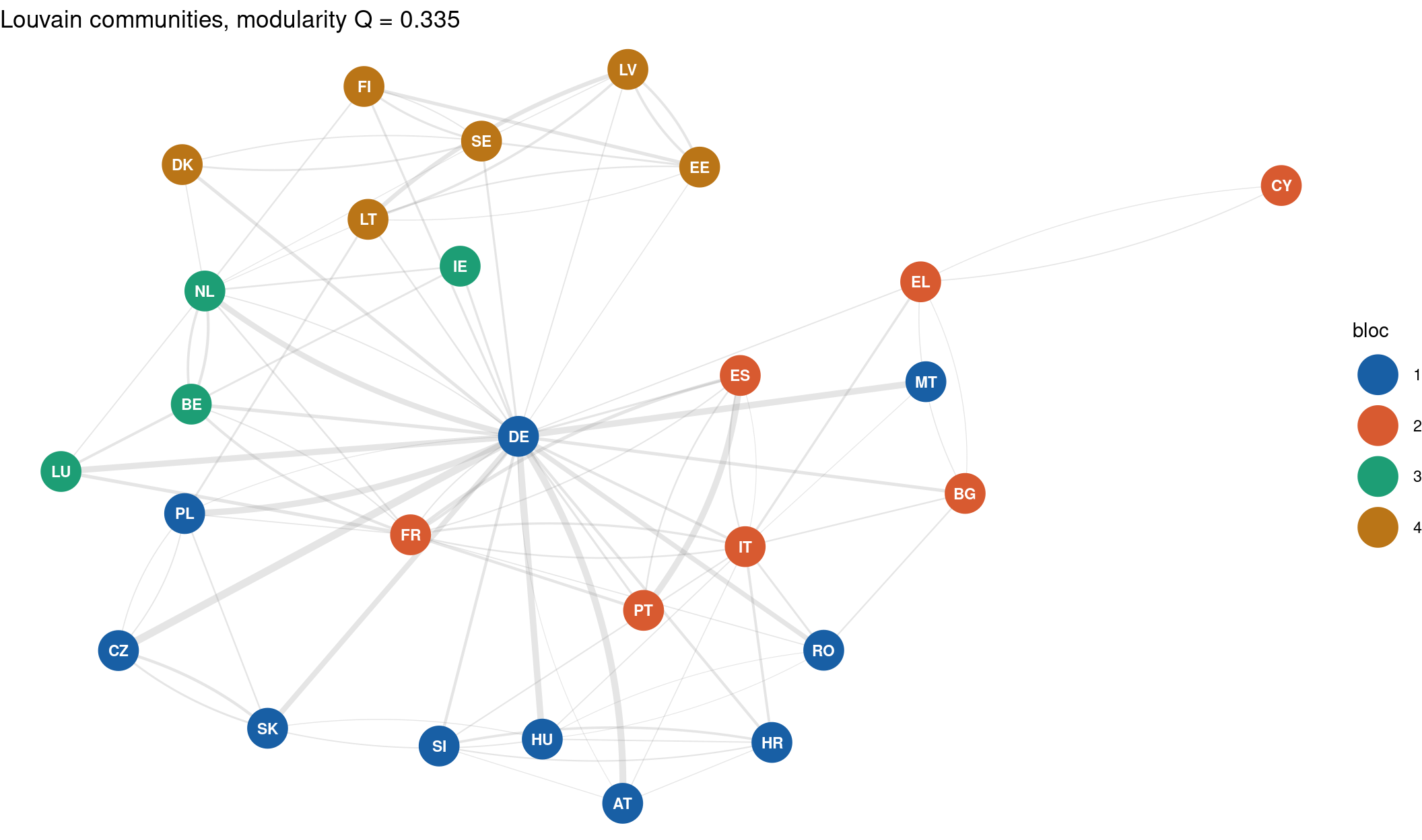
modularity Q = 0.335
Code
for i, b in enumerate(blocs, 1):
    print(f"bloc {i}:", sorted(b))
bloc 1: ['AT', 'CZ', 'DE', 'HR', 'HU', 'MT', 'PL', 'RO', 'SI', 'SK']
bloc 2: ['BE', 'IE', 'LU', 'NL']
bloc 3: ['BG', 'CY', 'EL', 'ES', 'FR', 'IT', 'PT']
bloc 4: ['DK', 'EE', 'FI', 'LT', 'LV', 'SE']

Geography emerges from trade flows alone: a Central-European bloc anchored on Germany, a Benelux group, a Mediterranean group around France–Italy–Spain, and a Nordic–Baltic group — no coordinates were used.

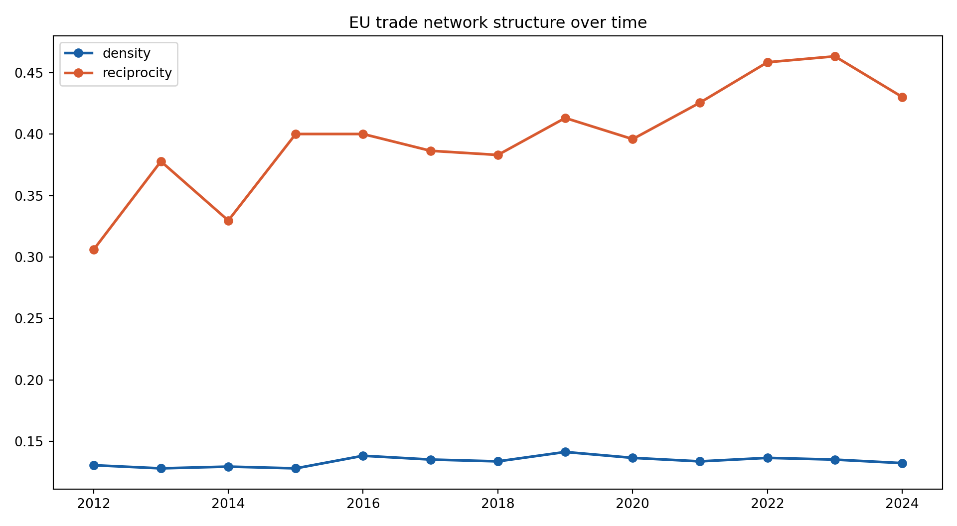
The Network over Time, 2012–2024

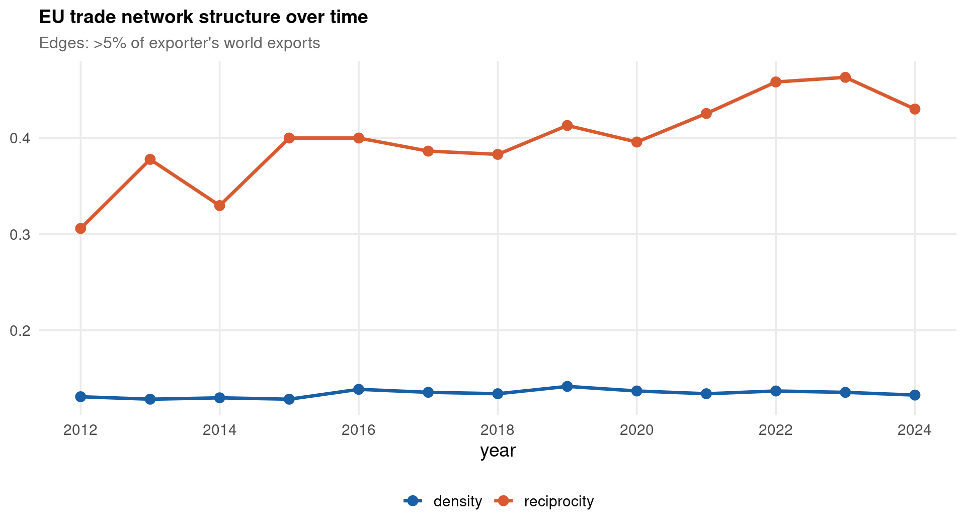
Did the EU trade network become denser and more reciprocal?

Code
years <- sort(unique(edges_all$time))
dens <- numeric(length(years))
rec  <- numeric(length(years))
for (i in seq_along(years)) {
  ey <- edges_all %>% filter(time == years[i], share > 5)
  gy <- graph_from_data_frame(ey %>% select(from, to), directed = TRUE)
  dens[i] <- edge_density(gy)
  rec[i]  <- reciprocity(gy)
}
ts <- data.frame(year = years, density = dens, reciprocity = rec)
ggplot(ts, aes(x = year)) +
  geom_line(aes(y = density,     color = "density"),     linewidth = 1.2) +
  geom_line(aes(y = reciprocity, color = "reciprocity"), linewidth = 1.2) +
  geom_point(aes(y = density,     color = "density"),     size = 3) +
  geom_point(aes(y = reciprocity, color = "reciprocity"), size = 3) +
  scale_color_manual(values = c(density = "#185FA5",
                                reciprocity = "#D85A30"), name = NULL) +
  scale_x_continuous(breaks = seq(2012, 2024, 2)) +
  labs(y = NULL, title = "EU trade network structure over time",
       subtitle = "Edges: >5% of exporter's world exports")

Code
rows = []
for yr in sorted(edges.time.unique()):
    ey = edges[(edges.time == yr) & (edges.share > 5)]
    Gy = nx.from_pandas_edgelist(ey, "from_c", "to_c",
                                 create_using=nx.DiGraph)
    rows.append([yr, nx.density(Gy), nx.reciprocity(Gy)])
ts = pd.DataFrame(rows, columns=["year", "density", "reciprocity"])
_ = plt.figure(figsize=(10, 5.5))
_ = plt.plot(ts.year, ts.density, "o-", color="#185FA5",
             linewidth=2, label="density")
_ = plt.plot(ts.year, ts.reciprocity, "o-", color="#D85A30",
             linewidth=2, label="reciprocity")
_ = plt.legend(); _ = plt.title("EU trade network structure over time")
plt.tight_layout()
plt.show()

Networks Meet Modern Trade Theory

  • Gravity explains flow sizes; networks explain the architecture of who-trades-with-whom. Head & Mayer (2014), Handbook of International Economics 4. doi:10.1016/B978-0-444-54314-1.00003-3
  • Chaney (2014): firms find new markets through existing contacts — trade networks grow by “friend-of-a-friend” dynamics, generating the observed geographic diffusion of exports. doi:10.1257/aer.104.11.3600
  • Production networks: sectoral shocks travel along input-output edges; asymmetric networks (hubs!) turn micro shocks into aggregate volatility — Acemoglu et al. (2012). doi:10.3982/ECTA9623
  • Global value chains: upstreamness/downstreamness are path-based network measures on the world input-output matrix — Antràs & Chor (2022), Handbook of International Economics 5. doi:10.1016/bs.hesint.2022.02.005
  • Supply-chain resilience: Covid and the Suez blockage renewed interest in centrality-as-vulnerability — Baldwin & Freeman (2022), Annual Review of Economics 14, 153–180. doi:10.1146/annurev-economics-051420-113737

Reading strategy: use network statistics as measurement (dependent or explanatory variables), and gravity/GE trade models as theory — the strongest papers do both.

Part V — Testing Network Structure

Reciprocity Test against the Erdős–Rényi Null

Is EU trade more two-way than chance?

  • Under \(G(n,p)\) with \(\hat{p} = L/[n(n-1)]\), each edge’s reverse exists independently with probability \(\hat{p}\), so the null expectation of reciprocity is \(\hat{p}\) itself
  • A raw reciprocity of \(0.46\) means nothing by itself — in a dense network even random edges reciprocate often
  • The test asks whether mutual trade dependence is structural

Test statistic, with \(\hat{r} = L^{\leftrightarrow}/L\):

\[ z = \frac{\hat{r} - \hat{p}}{\sqrt{\hat{p}(1-\hat{p}) / L}} \]

Reject the random null when:

\[ |z| > z_{0.975} = 1.96 \quad (\alpha = 0.05, \text{ two-sided}) \]

Code
L     <- ecount(g_eu)
n     <- vcount(g_eu)
p_hat <- edge_density(g_eu)
r_hat <- reciprocity(g_eu)
z     <- (r_hat - p_hat) / sqrt(p_hat * (1 - p_hat) / L)
p_val <- 2 * (1 - pnorm(abs(z)))
observed reciprocity : 0.463 
ER null (density)    : 0.135 
z statistic          : 9.34 
p-value              : <2e-16 
criterion            : reject if |z| > 1.96
verdict: REJECT the random null -- trade reciprocity is structural
Code
from scipy import stats
L = G_eu.number_of_edges()
p_hat = nx.density(G_eu)
r_hat = nx.reciprocity(G_eu)
z = (r_hat - p_hat) / np.sqrt(p_hat * (1 - p_hat) / L)
p_val = 2 * (1 - stats.norm.cdf(abs(z)))
print("observed reciprocity :", round(r_hat, 3))
print("ER null (density)    :", round(p_hat, 3))
print("z statistic          :", round(z, 2))
print("p-value              :", f"{p_val:.3g}")
print("criterion            : reject if |z| > 1.96")
print("verdict:",
      "REJECT the random null -- reciprocity is structural"
      if abs(z) > 1.96 else "cannot reject the random null")

Clustering Test — Monte Carlo against \(G(n,p)\)

Is the EU network more clustered than a random graph of the same density?

  • No closed-form null distribution for transitivity in small graphs — so we simulate it (a conditional uniform graph test)
  • Clustering rises mechanically with density; the correct question is “conditional on density, is the transitivity surprising?”
  • Draw \(B\) random graphs at the observed density, recompute clustering, and see where the observed value lands

Simulate \(B\) benchmark graphs and recompute clustering:

\[ C^{(b)} = C\!\left(G^{(b)}\right), \quad G^{(b)} \sim G(n, \hat{p}_u), \quad b = 1, \dots, B \]

Monte Carlo p-value, reject when \(p < \alpha = 0.05\):

\[ p = \frac{1}{B} \sum_{b=1}^{B} \mathbf{1}\!\left\{ C^{(b)} \geq C_{\text{obs}} \right\} \]

Code
set.seed(14159)
n_u   <- vcount(g_eu_u)
p_u   <- ecount(g_eu_u) / (n_u * (n_u - 1) / 2)
C_obs <- transitivity(g_eu_u)
B     <- 500
C_sim <- numeric(B)
for (b in 1:B) {
  C_sim[b] <- transitivity(sample_gnp(n_u, p_u))
}
p_mc <- mean(C_sim >= C_obs)
observed transitivity : 0.358 
ER mean (simulated)   : 0.205 
Monte Carlo p-value   : 0  (B = 500 )
criterion             : reject if p < 0.05
verdict: REJECT randomness -- clustering exceeds the ER null
Code
rng = np.random.default_rng(14159)
n_u = G_u.number_of_nodes()
p_u = G_u.number_of_edges() / (n_u * (n_u - 1) / 2)
C_obs = nx.transitivity(G_u)
B = 500
C_sim = np.empty(B)
for b in range(B):
    Gb = nx.gnp_random_graph(n_u, p_u, seed=int(rng.integers(1e9)))
    C_sim[b] = nx.transitivity(Gb)
p_mc = float(np.mean(C_sim >= C_obs))
print("observed transitivity :", round(C_obs, 3))
print("ER mean (simulated)   :", round(C_sim.mean(), 3))
print("Monte Carlo p-value   :", round(p_mc, 3), f"(B = {B})")
print("criterion             : reject if p < 0.05")
print("verdict:",
      "REJECT randomness -- clustering exceeds the ER null"
      if p_mc < 0.05 else
      "cannot reject -- clustering is compatible with the ER null")

Power-Law Degree Distribution Test (Clauset–Shalizi–Newman)

Do trade hubs follow a scale-free law \(P(k) \sim k^{-\alpha}\)? The CSN procedure (Clauset, Shalizi & Newman, 2009, doi:10.1137/070710111):

  • “Scale-free” claims are routinely made from eyeballing log-log plots; CSN showed most fail a formal test
  • Fit the tail by maximum likelihood, then judge the fit with a Kolmogorov–Smirnov distance and a bootstrap p-value
  • Economics alternative: the log rank-size regression with the Gabaix–Ibragimov \((\text{rank}-\tfrac{1}{2})\) correction (doi:10.1198/jbes.2009.06157) — Zipf’s law econometrics

Maximum likelihood exponent (for \(k \geq k_{\min}\)):

\[ \hat{\alpha} = 1 + n_{\text{tail}} \left[ \sum_{i=1}^{n_{\text{tail}}} \ln \frac{k_i}{k_{\min} - \tfrac{1}{2}} \right]^{-1} \]

Kolmogorov–Smirnov distance between empirical and fitted tail CDFs:

\[ D = \max_{k \geq k_{\min}} \left| \hat{F}(k) - F_{\hat{\alpha}}(k) \right| \]

Reject the power law when \(p_{\text{KS}} < 0.05\) (small \(p \Rightarrow\) the law fits badly).

Code
deg_in <- degree(g_eu, mode = "in")
deg_in <- deg_in[deg_in > 0]
set.seed(14159)
fit <- fit_power_law(deg_in, p.value = TRUE)   # CSN / plfit
alpha (MLE)   : 2.17 
k_min         : 2 
KS statistic  : 0.08 
KS p-value    : 0.606 
criterion     : reject power law if p < 0.05
verdict: power law NOT rejected (but see the warning below!)
Code
deg_in = np.array([d for _, d in G_eu.in_degree() if d > 0])
kmin = 2
tail = deg_in[deg_in >= kmin]
n_t = len(tail)
alpha = 1 + n_t / np.sum(np.log(tail / (kmin - 0.5)))
# KS distance against the fitted continuous power law
xs = np.sort(tail)
F_emp = np.arange(1, n_t + 1) / n_t
F_fit = 1 - (xs / kmin) ** (1 - alpha)
D = np.max(np.abs(F_emp - F_fit))
D_crit = 1.36 / np.sqrt(n_t)          # approximate 5% KS critical value
print("alpha (MLE)  :", round(alpha, 2), " (k_min =", kmin, ")")
print("KS statistic :", round(D, 3))
print("5% critical  :", round(D_crit, 3))
print("criterion    : reject power law if D > critical value")
print("verdict:",
      "REJECT the power law" if D > D_crit
      else "power law NOT rejected (small n -- weak evidence!)")

Part VI — Variations

Variation — Threshold Sensitivity

Every binarized result should survive a threshold change. Recompute the key statistics at 2%, 5% and 10%:

Code
thresholds <- c(2, 5, 10)
res <- data.frame()
for (th in thresholds) {
  et <- edges_all %>% filter(time == 2023, share > th)
  gt <- graph_from_data_frame(et %>% select(from, to), directed = TRUE)
  res <- rbind(res, data.frame(
    threshold   = th,
    edges       = ecount(gt),
    density     = round(edge_density(gt), 3),
    reciprocity = round(reciprocity(gt), 3),
    top_in      = names(sort(degree(gt, mode = "in"),
                             decreasing = TRUE))[1]))
}
res
 threshold edges density reciprocity top_in
         2   207   0.295       0.464     DE
         5    95   0.135       0.463     DE
        10    42   0.065       0.143     DE
Code
rows = []
for th in [2, 5, 10]:
    et = edges[(edges.time == 2023) & (edges.share > th)]
    Gt = nx.from_pandas_edgelist(et, "from_c", "to_c",
                                 create_using=nx.DiGraph)
    top = max(dict(Gt.in_degree()).items(), key=lambda x: x[1])[0]
    rows.append([th, Gt.number_of_edges(),
                 round(nx.density(Gt), 3),
                 round(nx.reciprocity(Gt), 3), top])
print(pd.DataFrame(rows, columns=["threshold", "edges", "density",
                                  "reciprocity", "top_in"]).to_string())

Germany stays the hub at every cutoff — the qualitative story is robust; the level of density and reciprocity is not. Report both.

Variation — Sectoral Networks

ext_tec03 also splits flows by NACE sector: B-E (industry) vs G (distribution/trade services). Do the two layers have the same architecture?

Code
sector_net <- function(nace_code) {
  st <- trade %>%
    filter(unit == "THS_EUR", stk_flow == "EXP", nace_r2 == nace_code,
           time == 2023, geo %in% eu27, partner %in% eu27,
           geo != partner, !is.na(values))
  sw <- trade %>%
    filter(unit == "THS_EUR", stk_flow == "EXP", nace_r2 == nace_code,
           time == 2023, geo %in% eu27, partner == "WORLD") %>%
    select(geo, world = values)
  st <- st %>% inner_join(sw, by = "geo") %>%
    mutate(share = 100 * values / world) %>% filter(share > 5)
  graph_from_data_frame(st %>% select(geo, partner), directed = TRUE)
}
g_ind <- sector_net("B-E")   # industry
g_srv <- sector_net("G")     # distribution & trade services
INDUSTRY (B-E)  : edges = 90  density = 0.138  reciprocity = 0.289 
  top in-degree :
DE IT FR NL BE 
25 11 10  8  6 
DISTRIBUTION (G): edges = 99  density = 0.141  reciprocity = 0.505 
  top in-degree :
DE IT FR NL PL 
22 10  9  7  7 
Code
def sector_net(nace_code):
    st = trade[(trade.unit == "THS_EUR") & (trade.stk_flow == "EXP")
               & (trade.nace_r2 == nace_code) & (trade.time == 2023)
               & (trade.geo.isin(eu27)) & (trade.partner.isin(eu27))
               & (trade.geo != trade.partner)].dropna(subset=["values"])
    sw = trade[(trade.unit == "THS_EUR") & (trade.stk_flow == "EXP")
               & (trade.nace_r2 == nace_code) & (trade.time == 2023)
               & (trade.geo.isin(eu27)) & (trade.partner == "WORLD")]
    sw = sw[["geo", "values"]].rename(columns={"values": "world"})
    st = st.merge(sw, on="geo")
    st["share"] = 100 * st["values"] / st["world"]
    st = st[st.share > 5]
    return nx.from_pandas_edgelist(st, "geo", "partner",
                                   create_using=nx.DiGraph)

for code, name in [("B-E", "INDUSTRY"), ("G", "DISTRIBUTION")]:
    Gs = sector_net(code)
    top = sorted(dict(Gs.in_degree()).items(), key=lambda x: -x[1])[:3]
    print(f"{name:14s}: edges={Gs.number_of_edges()}, "
          f"density={nx.density(Gs):.3f}, "
          f"reciprocity={nx.reciprocity(Gs):.3f}, top={top}")

Variations — Further Ideas

  • Imports instead of exports (stk_flow == "IMP"): does the import network have the same hubs? Correlate in-strength across the two
  • Maximum spanning tree backbone: keep the \(n-1\) strongest edges that connect everyone — the skeleton of EU trade
  • Add the neighbours: geo also covers CH, NO, UK, TR — how does Brexit-era UK sit in the network over 2012–2024?
  • Enterprise counts (unit == "NR_ENT"): a network of how many firms trade, not how much — extensive vs intensive margin
  • Multilayer view: treat each NACE sector as a layer; compare centrality rankings across layers
  • Rolling communities: run Louvain year by year — are blocs stable over 2012–2024?
  • Weighted throughout: redo the whole analysis with no threshold using strength and weighted PageRank only

Exercises — Estimation

  1. Rebuild the 2023 network with a 2% threshold and recompute in-degree, in-strength and PageRank. Which countries change rank the most, and why?
  2. Construct the import network (stk_flow == "IMP") for 2023 and compare its top-5 in-strength countries with the export network’s.
  3. Compute out-degree over time for Greece (EL) 2012–2024. Does its export diversification inside the EU rise or fall?
  4. Compute weighted betweenness using \(1/w_{ij}\) distances for all 27 countries in 2019 and 2023. Which country’s intermediation role changed most?
  5. Build the network on enterprise counts (unit == "NR_ENT", shares of the country’s world total) and correlate its in-strength ranking with the euro-value ranking (Spearman).
  6. Estimate the Katz–Bonacich vector \(b = (I - \phi A)^{-1}\mathbf{1}\) on the binarized 2023 network for \(\phi = 0.5/\lambda_{\max}\) and \(\phi = 0.9/\lambda_{\max}\), using solve() in R or np.linalg.solve in Python. How sensitive is the ranking to \(\phi\)?
  7. Extract the maximum spanning tree of the collapsed weighted network (mst() on negative weights in igraph) and plot it. Which edges form the backbone?
  8. Run Louvain for every year 2012–2024 with a fixed seed. Report the modularity time series and the years in which bloc membership changes.

Exercises — Testing

  1. Repeat the reciprocity z-test at thresholds 2%, 5% and 10%. Is the rejection robust?
  2. Repeat the clustering Monte Carlo test with \(B = 5000\) replications. Does the p-value change materially from \(B = 500\)?
  3. Design a Monte Carlo test for assortativity: is the EU network’s degree assortativity significantly negative compared to \(G(n, \hat{p})\)?
  4. Apply the CSN power-law test to the out-strength distribution (a continuous variable) instead of in-degree. Compare \(\hat{\alpha}\) and the KS p-value.
  5. Run the Gabaix–Ibragimov rank-size regression in all three languages for 2013 and 2023, and test whether \(\hat{\alpha}\) changed between the two years.
  6. Simulate 500 directed ER graphs with the same \(n\) and \(L\) and compare the observed maximum in-degree (Germany’s 25) with the simulated distribution. What is the Monte Carlo p-value of such a hub arising by chance?
  7. Use a degree-preserving rewiring null (rewire(g, keeping_degseq(niter = 1000)) in igraph) instead of ER for the clustering test. Does the conclusion survive when hubs are kept fixed?
  8. Test whether the Louvain partition beats chance: permute country labels 500 times, recompute modularity of the permuted partition, and compare with \(Q_{\text{obs}}\).

Further Reading

Thank You

Athanassios Stavrakoudis
Applied Informatics and Computational Economics Lab
Department of Economics
University of Ioannina, Greece

astavrak@uoi.gr · linkedin.com/in/astavrakoudis