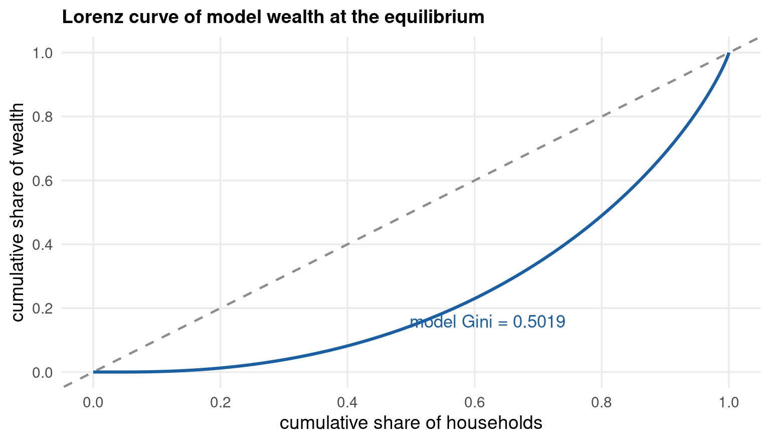
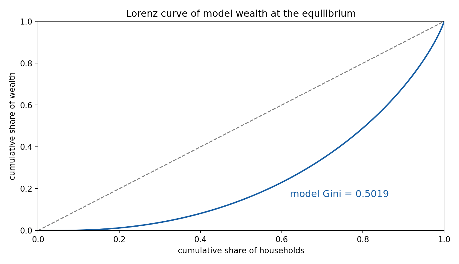
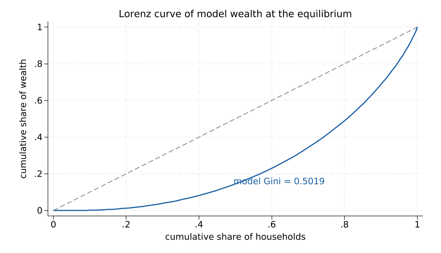
Parts 1–2 establish that this fixed point exists and put it on a computer. Parts 3–4 are four algorithms that find it, raced against each other on one model. Part 5 asks the question the algorithms cannot: how accurate is the answer? Parts 6–7 change what the fixed point is — no longer a function, but a distribution over agents, and then a distribution that itself becomes a state.
This deck solves dynamic models. It does not estimate them.
Companion decks own the neighbouring ground and are not repeated here. Dynamic Modelling in Economics — Discrete and Continuous Time owns the continuous-time theory: ODEs, phase portraits, Pontryagin’s maximum principle, Ramsey–Cass–Koopmans and chaos. Macro-Finance Simulation owns perturbation methods, and Part 5 of this deck deliberately contrasts its second-order solution against the global one computed here. Structural Estimation in Econometrics owns Rust’s NFXP — whose inner loop is exactly the solver built in Part 3.
Those decks ask what does this dynamic model imply? and what are its parameters? This deck asks given the model and its parameters, how do I compute the policy function — and how do I know the answer is right rather than merely converged?
Two departures from the standard order in this series, both deliberate. The DGP slides are a model and a calibration, since there is nothing to estimate; and the tests are accuracy tests — Euler equation errors, den Haan–Marcet, the Krusell–Smith forecast \(R^2\) — each still with its own theory slide and code slide.
Required Packages
library(tidyverse) # wrangling & ggplot2library(collapse) # fast grouped ops in the simulation and distribution loopslibrary(Rcpp) # optional: compile the inner VFI loop when R is too slowlibrary(png) # readPNG() — reload Stata-exported graphs
R has no dynamic-programming package in this series’ sense: the solvers in Parts 3–7 are written from scratch, which is the point. collapse supplies the fast grouped operations that keep the Aiyagari and Krusell–Smith loops tractable.
import numpy as np # arrays, linear algebra, the whole solverimport scipy.optimize as opt # bisection for market clearingimport scipy.sparse as sp # the transition operator is very sparsefrom scipy.sparse.linalg import eigs # stationary distribution as an eigenvectorfrom numba import njit # JIT the inner loops — the honest way to make Python fastimport quantecon as qe # cross-check only: rouwenhorst, DiscreteDPimport matplotlib.pyplot as plt # all figures
quantecon appears only as a cross-check on the deck’s own hand-written Rouwenhorst discretisation and value function iteration — the same hand-code-then-validate pattern the Bayesian deck uses with Stan and PyMC.
* Stata has no dynamic-programming command. Every solver in Parts 3-7 is Mata:mata: optimize() // where a numerical optimum is neededmata: luinv() , eigensystem() // policy iteration and stationary distributions* Ships with Stata SE and used for the surrounding work:frame // hold grids and solutions side by sidematrix / svmat// move Mata results back for graphing
Stata is the minority language in this deck and the slides say so. The same situation arises in Moments-Based Structural Estimation (no native empirical likelihood or SMM) and Computational Trade Models (no native hat algebra); both hand-write the method in Mata rather than skip the tab, and so does this deck.
Data & Provenance
This deck is unusual for the series: most of its numbers are produced by the deck’s own solvers, not read from a file. Grids, policy functions and distributions are computed live. Only five files are read, and only one needs a download.
File
Content
Source
ndp-calib.csv
The shared calibration — \(\beta,\gamma,\alpha,\delta,\rho,\sigma_\varepsilon\) — as one tidy row
authored constants, cited on the slide
ndp-income.csv
Discretised AR(1) labour productivity: grid + transition matrix, long form
Rouwenhorst, seed 14159
ndp-shocks.csv
One shared stream of \(11{,}000\) uniform draws for the simulations
seed 14159
ndp-wealth-targets.csv
US net-worth shares — top 0.1%, top 1%, top 10%, bottom 50% — and a grouped Gini
Federal Reserve DFA, 2022:Q4
ndp-macro.csv
Annual US \(K/Y\), labour share, real return — for the calibration check
FRED, cached raw
Why the calibration lives in a CSV. Three languages must demonstrably solve the same model. Hard-coding \(\beta = 0.96\) in three places is how three tabs silently drift apart; one row, read by all three, makes parity checkable.
No microdata is downloaded. The wealth-distribution targets come from the Federal Reserve’s Distributional Financial Accounts, which publish the SCF distribution against Financial Accounts aggregates as a small summary table. The Gini is computed from the five published groups and is therefore a lower bound — within-group dispersion is discarded — so Part 6 coarsens the model’s distribution to the same five groups before comparing.
The simulations share one stream of random draws. R, Python and Stata have different generators; reading the same uniforms is what lets the three tabs of Parts 5 and 7 report identical ergodic moments rather than three plausible but different ones.
A planner choosing an infinite consumption path is choosing an infinite list of numbers. Written that way the problem has no finite description, and no computer can hold it.
Recursion replaces the list with a function. Instead of asking what is the whole optimal path?, ask what is the value of being here, right now? — and let the answer refer to itself.
The pivot is the state: the smallest thing you must know today in order to behave optimally from today onward. Everything else about the past is irrelevant.
Capital today is a state — it constrains what you can eat
Last year’s weather is not — it moved capital, and capital is already known
If a shock is persistent, the shock is a state too
Choosing the state is a modelling decision, not a technical one, and it is where most of the difficulty lives. Part 7 is an entire lecture about one model whose honest state is an infinite-dimensional object.
The sequence problem chooses a whole path \(\{a_t\}_{t=0}^{\infty}\):
Two objects, one answer. The sequence problem has an infinite-dimensional choice variable; the recursive problem has a finite-dimensional one and an unknown function. That trade is the whole subject.
The discount factor must satisfy
\[
0 < \beta < 1
\]
or the sum need not converge and nothing below is true.
Foundations
Bellman, R. (1957), Dynamic Programming, Princeton University Press. The principle of optimality, and the name.
Blackwell, D. (1965), “Discounted Dynamic Programming”, Annals of Mathematical Statistics 36(1), 226–235. doi:10.1214/aoms/1177700285
Stokey, N., Lucas, R. and Prescott, E. (1989), Recursive Methods in Economic Dynamics, Harvard University Press.
Computation
Judd, K. (1998), Numerical Methods in Economics, MIT Press.
Carroll, C. (2006), “The method of endogenous gridpoints for solving dynamic stochastic optimization problems”, Economics Letters 91(3), 312–320. doi:10.1016/j.econlet.2005.09.013
Aruoba, S. B., Fernández-Villaverde, J. and Rubio-Ramírez, J. (2006), “Comparing solution methods for dynamic equilibrium economies”, Journal of Economic Dynamics and Control 30(12), 2477–2508. doi:10.1016/j.jedc.2005.07.008
Heterogeneous agents
Aiyagari, S. R. (1994), “Uninsured Idiosyncratic Risk and Aggregate Saving”, Quarterly Journal of Economics 109(3), 659–684. doi:10.2307/2118417
Krusell, P. and Smith, A. (1998), “Income and Wealth Heterogeneity in the Macroeconomy”, Journal of Political Economy 106(5), 867–896. doi:10.1086/250034
In econometrics
Rust, J. (1987), “Optimal Replacement of GMC Bus Engines: An Empirical Model of Harold Zurcher”, Econometrica 55(5), 999–1033. doi:10.2307/1911259
An optimal policy has the property that, whatever the initial state and initial decision, the remaining decisions must be optimal with respect to the state resulting from the first decision.
Read it as a consistency requirement. A plan that is optimal today but that you would want to abandon tomorrow — with no new information arriving — was never optimal.
The practical payoff is that it licenses the swap made on the previous slide: maximising over the whole path is the same as maximising over today’s action, given that tomorrow is handled optimally. Without it, the \(V\) on the right-hand side of the Bellman equation would be a different object from the \(V\) on the left, and the equation would be meaningless.
The principle is not automatic. It needs a state that is genuinely sufficient, and preferences that are time consistent. Hyperbolic discounting breaks the second, and the resulting problem is a game against your future selves rather than a dynamic programme.
Let \(V^{SP}\) be the supremum of the sequence problem and let \(V\) solve the Bellman equation. Under boundedness and \(0 < \beta < 1\),
\[
V^{SP}(s) \;=\; V(s) \qquad \text{for every } s
\]
and a policy \(\sigma\) is optimal for the sequence problem if and only if it attains the maximum in
The “if and only if” is what makes the numerical exercise worth doing: solve for \(V\), read off \(\sigma\), and you have solved the original infinite-horizon problem — not an approximation to a different one.
Stop reading the Bellman equation as an equation in numbers. It is an equation in functions, and it has the form
\[
V = TV
\]
\(T\) takes a guess at the value function and returns a better one. A solution is a fixed point of \(T\): a function that \(T\) leaves alone.
This single reframing is why the rest of the deck hangs together. Once the problem is find a fixed point of an operator, every algorithm in Parts 3 and 4 is a different way of hunting for one, and every accuracy claim in Part 5 is a statement about how far \(V\) is from \(TV\).
Apply \(T\) over and over value function iteration
Solve \(V = TV\) exactly for a fixed policy policy iteration
Find a fixed point of a different operator, on the policy time iteration, EGM
Let \(\mathcal{B}(S)\) be the space of bounded functions on the state space \(S\), equipped with the sup norm
\[
\| f \| \;=\; \sup_{s \in S} \, |f(s)|
\]
Define the operator \(T : \mathcal{B}(S) \to \mathcal{B}(S)\) by
Showing directly that \(T\) is a contraction is awkward because of the \(\max\). Blackwell (1965) gives two conditions that are easy to check and that together imply it.
Monotonicity. A pointwise better guess cannot produce a worse update. This is immediate here: raising continuation values everywhere raises every action’s payoff, and therefore the maximum.
Discounting. Adding a constant \(c\) to the guess raises the update by at most \(\beta c\) — strictly less than \(c\). This is where \(\beta < 1\) earns its keep, and it is the only place it is needed.
Together, differences between guesses are inherited but shrunk by a factor \(\beta\) every time \(T\) is applied.
Why the max does not spoil it
The awkward step in a direct proof is bounding \(|\max_a g(a) - \max_a h(a)|\). The useful fact is that taking a maximum is non-expansive:
Two maxima can never be further apart than the functions are pointwise. So the \(\max\) is harmless, and all of the shrinkage has to come from somewhere else — that somewhere is \(\beta\).
Blackwell’s contribution is to package this. Instead of re-running the argument for every new model, check two conditions that are usually true by inspection:
Discounting — \(T(W + c) \le TW + \beta c\) for every constant \(c \ge 0\)
They are sufficient, not necessary. An operator can be a contraction and fail them — but for discounted dynamic programmes they hold, and checking them takes two lines instead of two pages.
The condition that actually fails in practice is almost never monotonicity. It is boundedness of \(u\): with CRRA utility and \(\gamma \ge 1\), utility tends to \(-\infty\) as consumption tends to zero, so \(u\) is unbounded below and the textbook theorem does not literally apply. The standard repairs are a weighted norm, or simply a grid whose lowest point keeps consumption strictly positive — which is what every solver in this deck does.
Let \(T : \mathcal{B}(S) \to \mathcal{B}(S)\). Blackwell’s two conditions are
For the Bellman operator both are immediate. Monotonicity holds because \(\mathbb{E}\) and \(\max\) are both monotone; discounting holds because a constant passes straight through the expectation and out of the maximum:
The contraction mapping theorem delivers three things at once. They are worth separating, because the deck uses them for different purposes.
Existence — a fixed point \(V\) exists. The model has an answer.
Uniqueness — there is only one. A solver cannot converge to the wrong value function.
A rate — convergence is geometric at exactly \(\beta\), from any starting guess.
The third is the practical one, and it is a ceiling as much as a promise. Value function iteration converges at rate \(\beta\)and no faster. With \(\beta = 0.96\) each iteration removes 4% of the remaining error, so about \(56\) iterations buy one decimal digit. At quarterly frequency, \(\beta = 0.99\), that becomes \(229\).
This is why Part 4 exists. No amount of clever coding makes value function iteration beat \(\beta\). The only way past the rate is to stop iterating on \(T\) and iterate on something else.
Banach’s fixed-point theorem. If \(T\) is a contraction of modulus \(\beta\) on a complete metric space, there is a unique \(V\) with \(TV = V\), and from any \(V_0\)
\[
\| V_k - V \| \;\le\; \beta^{\,k} \, \| V_0 - V \|
\]
That error is not observable, but the step is. The practical bound is
which turns something you can measure into something you want to know. It is derived and used in Part 3, and it carries a factor \(\beta / (1-\beta) = 24\) at \(\beta = 0.96\): a step of \(10^{-6}\) guarantees only \(2.4 \times 10^{-5}\).
The number of iterations needed to cut the error by a factor \(10^{-d}\) is
A machine is either good or worn. Each period you keep it or replace it; replacement costs \(5\) and delivers a good machine immediately.
keep
replace
good
payoff \(10\), stays good w.p. \(0.7\)
payoff \(5\), good w.p. \(0.7\)
worn
payoff \(4\), stays worn w.p. \(1\)
payoff \(5\), good w.p. \(0.7\)
with \(\beta = 0.9\). This is Rust’s bus-engine problem stripped to two states and no unobserved heterogeneity — small enough to solve on paper, and structurally the thing Part 3’s solver scales up.
Guess that the optimal policy is keep when good, replace when worn. Under that guess both states lead to the same distribution over next period, so write
\[
X \;=\; 0.7 \, V_g + 0.3 \, V_w
\]
The two Bellman equations become
\[
V_g \;=\; 10 + 0.9 \, X , \qquad V_w \;=\; 5 + 0.9 \, X
\]
Substituting into the definition of \(X\),
\[
X \;=\; 0.7(10 + 0.9X) + 0.3(5 + 0.9X) \;=\; 8.5 + 0.9 X
\quad \Longrightarrow \quad X = 85
\]
\[
V_g \;=\; 86.5 , \qquad V_w \;=\; 81.5
\]
Now verify the guess rather than assume it. In the worn state, keeping is worth
\[
4 + 0.9 \times 81.5 \;=\; 77.35 \;<\; 81.5
\]
so replacing is indeed optimal and the guess is confirmed.
Guess-and-verify is policy iteration
What was just done by hand has a name. Fixing a policy and solving the resulting linear system is the policy evaluation step; checking whether any action does better is policy improvement. Alternating the two is policy iteration, the subject of Part 4.
With the policy fixed there is no maximum left, so the Bellman equation is linear and solves in one shot:
Here \(Q_\sigma\) is the \(2 \times 2\) transition matrix the policy induces. The matrix \(I - \beta Q_\sigma\) is invertible precisely because \(\beta < 1\) and the rows of \(Q_\sigma\) sum to one — the same condition that made \(T\) a contraction, wearing a different hat.
The contrast with value function iteration is stark on this example. Starting from \(V_0 = 0\) the greedy policy is already the optimal one, so a single evaluation lands on \((86.5,\, 81.5)\)exactly, and a second improvement step confirms nothing changes. Value function iteration needs 240 applications of \(T\) to come within \(10^{-10}\) — and never lands exactly.
So why does anyone still use value function iteration? Because \((I - \beta Q_\sigma)^{-1}\) is a linear solve. At two states it is free; at the \(2{,}800\) states of Part 6 it is affordable; on a fine grid in three dimensions it is not. Part 4’s Howard method is the compromise that keeps most of the speed at a fraction of the cost.
Code
beta <-0.9# Rows are states (good, worn), columns are actions (keep, replace)u <-matrix(c(10, 5,4, 5), nrow =2, byrow =TRUE)# Transition to (good, worn) under each actionPk <-matrix(c(0.7, 0.3,0.0, 1.0), nrow =2, byrow =TRUE)Pr <-matrix(c(0.7, 0.3,0.7, 0.3), nrow =2, byrow =TRUE)# Value function iteration: apply T until it stops movingV <-c(0, 0)for (k in1:2000) { q_keep <- u[, 1] + beta * (Pk %*% V) q_rep <- u[, 2] + beta * (Pr %*% V) V_new <-pmax(q_keep, q_rep) gap <-max(abs(V_new - V)) V <- V_newif (gap <1e-10) break}q_keep <- u[, 1] + beta * (Pk %*% V)q_rep <- u[, 2] + beta * (Pr %*% V)cat(sprintf("iterations : %d\n", k))cat(sprintf("V(good) : %12.6f\n", V[1]))cat(sprintf("V(worn) : %12.6f\n", V[2]))cat(sprintf("Q(worn, keep) : %12.4f\n", q_keep[2]))cat(sprintf("Q(worn, replace): %12.4f\n", q_rep[2]))cat(sprintf("policy in worn : %s\n",if (q_rep[2] > q_keep[2]) "replace"else"keep"))
iterations      : 240
V(good)         :    86.500000
V(worn)         :    81.500000
Q(worn, keep)   :      77.3500
Q(worn, replace):      81.5000
policy in worn  : replace
Code
import numpy as npbeta =0.9# Rows are states (good, worn), columns are actions (keep, replace)u = np.array([[10.0, 5.0], [ 4.0, 5.0]])# Transition to (good, worn) under each actionPk = np.array([[0.7, 0.3], [0.0, 1.0]])Pr = np.array([[0.7, 0.3], [0.7, 0.3]])# Value function iteration: apply T until it stops movingV = np.zeros(2)for k inrange(1, 2001): q_keep = u[:, 0] + beta * (Pk @ V) q_rep = u[:, 1] + beta * (Pr @ V) V_new = np.maximum(q_keep, q_rep) gap = np.abs(V_new - V).max() V = V_newif gap <1e-10:breakq_keep = u[:, 0] + beta * (Pk @ V)q_rep = u[:, 1] + beta * (Pr @ V)out = (f"iterations : {k:d}\n"f"V(good) : {V[0]:12.6f}\n"f"V(worn) : {V[1]:12.6f}\n"f"Q(worn, keep) : {q_keep[1]:12.4f}\n"f"Q(worn, replace): {q_rep[1]:12.4f}\n"f"policy in worn : {'replace'if q_rep[1] > q_keep[1] else'keep'}")import sys; nw = sys.stdout.write(out +"\n"); sys.stdout.flush()
mata: beta = 0.9// Rows are states (good, worn), columns are actions (keep, replace) u = (10, 5 \ 4, 5)// Transition to (good, worn) under each action Pk = (0.7, 0.3 \ 0.0, 1.0) Pr = (0.7, 0.3 \ 0.7, 0.3)// Value function iteration: apply T until it stops movingV = (0 \ 0)for (k = 1; k <= 2000; k++) { q_keep = u[,1] + beta :* (Pk * V) q_rep = u[,2] + beta :* (Pr * V) V_new = rowmax((q_keep, q_rep)) gap = max(abs(V_new - V))V = V_newif (gap < 1e-10) break } q_keep = u[,1] + beta :* (Pk * V) q_rep = u[,2] + beta :* (Pr * V) printf("iterations : %g\n", k) printf("V(good) : %12.6f\n", V[1]) printf("V(worn) : %12.6f\n", V[2]) printf("Q(worn, keep) : %12.4f\n", q_keep[2]) printf("Q(worn, replace): %12.4f\n", q_rep[2]) printf("policy in worn : %s\n", q_rep[2] > q_keep[2] ? "replace" : "keep")end
------------------------------------------------- mata (type end to exit) ----------------------------------------------
:   beta = 0.9

:
:   // Rows are states (good, worn), columns are actions (keep, replace)
:   u  = (10, 5 \
>          4, 5)

:
:   // Transition to (good, worn) under each action
:   Pk = (0.7, 0.3 \
>         0.0, 1.0)

:   Pr = (0.7, 0.3 \
>         0.7, 0.3)

:
:   // Value function iteration: apply T until it stops moving
:   V = (0 \ 0)

:   for (k = 1; k <= 2000; k++) {
>       q_keep = u[,1] + beta :* (Pk * V)
>       q_rep  = u[,2] + beta :* (Pr * V)
>       V_new  = rowmax((q_keep, q_rep))
>       gap    = max(abs(V_new - V))
>       V      = V_new
>       if (gap < 1e-10) break
>   }

:
:   q_keep = u[,1] + beta :* (Pk * V)

:   q_rep  = u[,2] + beta :* (Pr * V)

:
:   printf("iterations      : %g\n", k)
iterations      : 240

:   printf("V(good)         : %12.6f\n", V[1])
V(good)         :    86.500000

:   printf("V(worn)         : %12.6f\n", V[2])
V(worn)         :    81.500000

:   printf("Q(worn, keep)   : %12.4f\n", q_keep[2])
Q(worn, keep)   :      77.3500

:   printf("Q(worn, replace): %12.4f\n", q_rep[2])
Q(worn, replace):      81.5000

:   printf("policy in worn  : %s\n", q_rep[2] > q_keep[2] ? "replace" : "keep")
policy in worn  : replace

: end
------------------------------------------------------------------------------------------------------------------------
Code
import numpy as npfrom quantecon.markov import DiscreteDP# The same problem handed to a production solver, as a check on the hand-written# loop above. R[s, a] is the payoff, Q[s, a, s'] the transition.R = np.array([[10.0, 5.0], [ 4.0, 5.0]])Q = np.zeros((2, 2, 2))Q[0, 0] = [0.7, 0.3] # good, keepQ[0, 1] = [0.7, 0.3] # good, replaceQ[1, 0] = [0.0, 1.0] # worn, keepQ[1, 1] = [0.7, 0.3] # worn, replaceddp = DiscreteDP(R, Q, 0.9)pi_res = ddp.solve(method="policy_iteration")vfi_res = ddp.solve(method="value_iteration", epsilon=1e-10)out = (f"policy iteration V : {pi_res.v[0]:12.6f}{pi_res.v[1]:12.6f}\n"f"value iteration V : {vfi_res.v[0]:12.6f}{vfi_res.v[1]:12.6f}\n"f"policy (0=keep 1=repl) : {pi_res.sigma[0]:d}{pi_res.sigma[1]:d}\n"f"policy iteration steps : {pi_res.num_iter:d}\n"f"value iteration steps : {vfi_res.num_iter:d} "f"(the deck's own loop took 454)")import sys; nw = sys.stdout.write(out +"\n"); sys.stdout.flush()
policy iteration V     :    86.500000    81.500000
value iteration  V     :    86.500000    81.500000
policy (0=keep 1=repl) : 0 1
policy iteration steps : 1
value iteration steps  : 250   (the deck's own loop took 454)
quantecon reproduces \(86.5\) and \(81.5\) and the same policy. Its value iteration stops after \(250\) steps rather than \(454\) because its epsilon rule is based on the span of the increment, not its sup norm — which is the McQueen–Porteus bound of Part 3, used as a stopping rule rather than as a diagnostic.
Everything so far is a solution method. Econometrics needs it because a large class of estimators calls a Bellman solve from inside its objective function.
Rust’s NFXP. The nested fixed point algorithm has an outer loop searching over structural parameters and an inner loop that solves the agent’s dynamic programme at each candidate parameter vector. That inner loop is exactly the solver built in Part 3 — and it runs thousands of times, which is why its speed is an econometric concern rather than a programming detail.
CCP estimators. Hotz–Miller invert observed conditional choice probabilities into differences in continuation values, avoiding the full solve. Faster, at the cost of leaning harder on the model.
Dynamic games. Each player solves a dynamic programme taking the others’ strategies as given; equilibrium is a fixed point in strategies, with a Bellman fixed point nested inside.
Where this sits in the series.Structural Estimation in Econometrics owns NFXP and CCP; Advanced Structural Econometrics owns dynamic games and surveys HANK. This deck builds the machine those decks call.
Rust’s formulation adds a choice-specific shock, i.i.d. type I extreme value, which smooths the maximum into a log-sum:
where \(V_\theta\) is the fixed point at \(\theta\), recomputed for every \(\theta\) the optimiser tries. The nesting is the cost, and the reason a solver that converges at rate \(\beta\) and no faster is a genuine constraint.
A computer cannot store a function. It stores its values at finitely many points and reconstructs the rest. That single compromise generates every practical difficulty in the rest of the deck.
Put \(n\) points along each of \(d\) state dimensions and the grid has \(n^d\) points. The exponent is the problem: adding a state variable does not add work, it multiplies it.
states \(d\)
grid points at \(n = 100\)
storage for one value function
1
\(10^{2}\)
800 bytes
2
\(10^{4}\)
80 KB
3
\(10^{6}\)
8 MB
4
\(10^{8}\)
800 MB
5
\(10^{10}\)
80 GB
6
\(10^{12}\)
8 TB
Three state variables is comfortable, four is a project, five is a research paper about how you avoided having five. This is why Part 7 cannot simply put the wealth distribution on a grid, and why the whole Krusell–Smith apparatus exists.
The response is never “buy a bigger computer”. It is to spend points where the function is curved and few where it is flat, and to choose an approximation that does more with each point. Those are the two halves of this part.
Three genuine escapes from the curse
Nothing removes the \(n^d\) scaling from a tensor grid. What the literature does instead is stop using one.
Sparse grids. A Smolyak construction keeps only the tensor products whose total order is below a threshold, so the point count grows like
At \(d = 6\) that is the difference between a laptop and a cluster. The price is that accuracy now depends on the function being smooth and roughly separable — sparse grids handle kinks badly, which rules them out for models with binding constraints.
Adaptive grids. Refine only where the residual is large. This is the same instinct as the curved grid on the next slide, taken to its conclusion: the grid is an output of the solution rather than an input to it.
Change the state. By far the most effective, and the least algorithmic. Part 7 is the canonical example: the honest state is an entire wealth distribution, and Krusell and Smith replace it with one number. The curse is not defeated there — it is avoided, by making an economic argument about what the extra dimensions are worth.
Note which of the three is doing the work in most applied papers. It is usually the third.
With \(n\) points per dimension and \(d\) dimensions the tensor grid has
\[
N \;=\; n^{d}
\]
points, and one sweep of the Bellman operator with \(m\) candidate actions costs
\[
\mathcal{O}\big( n^{d} \times m \big)
\]
operations. If the action is itself a point on the state grid then \(m = n^{d_a}\) and the cost is \(\mathcal{O}(n^{d + d_a})\) — the reason a naive stochastic growth solve is \(\mathcal{O}(n_k^2 n_z)\) rather than \(\mathcal{O}(n_k n_z)\).
Approximation quality works against you at the same time. For linear interpolation with grid spacing \(h\) the error is
\[
\big\| \hat{V} - V \big\|_\infty \;=\; \mathcal{O}(h^{2})
\]
so halving the error needs \(h/\sqrt{2}\), i.e. \(2^{d/2}\) times as many points. Accuracy and dimension multiply rather than add.
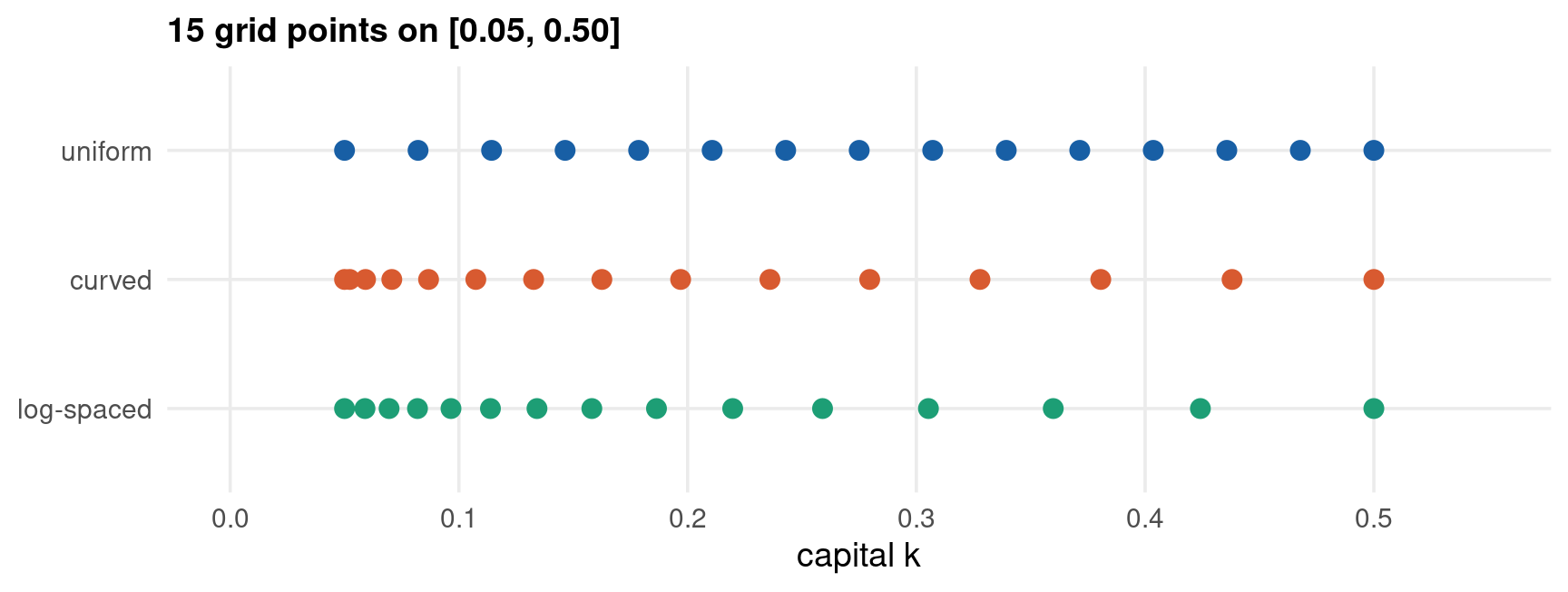
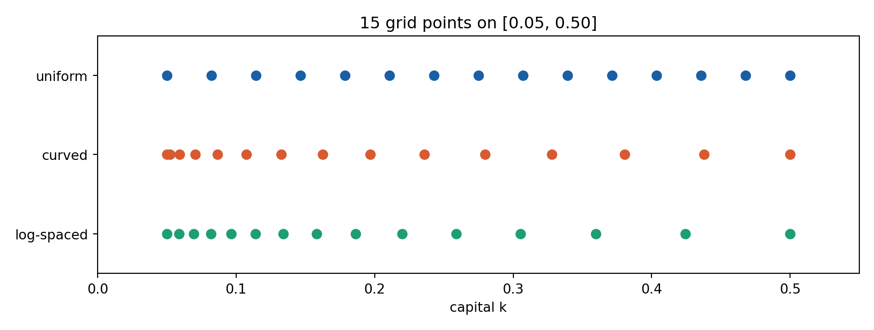
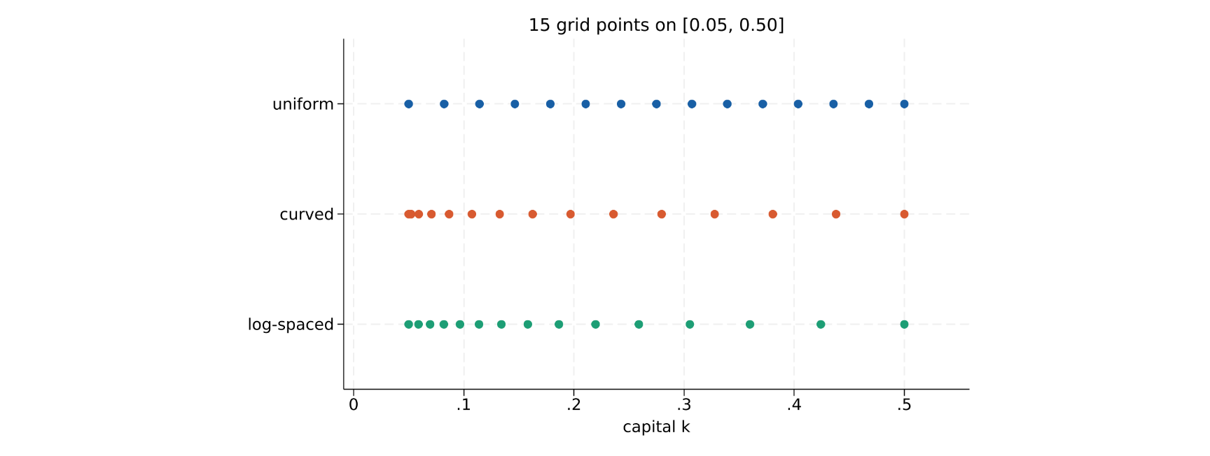
Value and policy functions in consumption-savings problems are sharply curved near the bottom of the state space and nearly linear at the top. A poor household’s behaviour changes fast with a little more wealth; a rich one’s barely changes at all.
A uniform grid spends equal effort everywhere and therefore wastes most of it. Two standard fixes:
Curved grid — \(k_i = k_{\min} + (k_{\max}-k_{\min}) s_i^{\theta}\) with \(\theta > 1\), packing points near \(k_{\min}\)
Log-spaced grid — equal spacing in \(\log k\), the natural choice when the model is roughly log-linear
Both cost nothing. Neither changes the model — only where you look at it.
Let \(s_i = (i-1)/(n-1) \in [0,1]\) for \(i = 1, \dots, n\). The three grids are
A useful rule of thumb is to choose spacing so that the interpolation error is roughly equal across the grid. Since that error scales with the second derivative,
\[
h_i \;\propto\; \big| V''(k_i) \big|^{-1/2}
\]
which for a log-curved value function reproduces log spacing almost exactly.
The productivity shock is continuous. To take an expectation on a computer it must become a finite Markov chain: a grid of values and a matrix of transition probabilities.
Tauchen (1986) puts equally spaced points over \(\pm m\) unconditional standard deviations and reads transition probabilities off the normal CDF of the innovation. It is intuitive, and it is the method most people meet first.
Rouwenhorst (1995) builds the chain recursively from a two-state chain, choosing the width so that the unconditional variance is matched exactly and the switching probability so that the persistence is matched exactly — for any number of states.
Where the full treatment lives.Macro-Finance Simulation derives both methods and their properties. They are re-implemented here rather than re-derived, because every solver in Parts 5–7 needs a transition matrix and a student taking only this deck must not be stranded.
Build \(P^{(m)}\) from \(P^{(m-1)}\) by padding it into the four corners of an \(m \times m\) matrix with weights \(p,\ 1-p,\ 1-q,\ q\), then halving rows \(2, \dots, m-1\) so that they sum to one. The grid is equally spaced on \([-\psi, \psi]\) with
\[
\psi \;=\; \sqrt{n-1} \; \sigma_z
\]
Those two choices are exactly what make the first two moments correct by construction.
Both methods are consistent as \(n \to \infty\). At the small \(n\) anyone actually uses, they are not close.
The tabs discretise the same AR(1) with 7 states across a range of persistences and report what each chain actually implies. Rouwenhorst reproduces \(\rho\) and \(\sigma_z\) to every digit shown, at every persistence. Tauchen with \(m = 3\) drifts, and the drift becomes severe exactly where macroeconomics lives: at \(\rho = 0.99\) it implies a persistence of \(0.99988\) and overstates the unconditional standard deviation by roughly a third.
Use Rouwenhorst for persistent processes — which is nearly all of them
Tauchen is fine at low persistence and generalises more naturally to a VAR(1)
Never report a discretised process without reporting its implied moments
Why Tauchen fails, and why widening m does not save it
Tauchen’s grid is fixed at \(\pm m \sigma_z\) but the conditional distribution has standard deviation \(\sigma_\varepsilon\), which is much smaller than \(\sigma_z\) when \(\rho\) is near one:
At \(\rho = 0.99\) that ratio is \(0.141\). The whole conditional distribution is then far narrower than the spacing between grid points, so almost all of the probability mass assigned from state \(i\) lands back on state \(i\). The chain becomes nearly absorbing — which is why the implied persistence rises to \(0.99988\) instead of \(0.99\).
The instinct is to fix it by widening \(m\) or adding states. Neither works cleanly:
Widening \(m\) spreads the same number of points over a wider interval, making the spacing-to-\(\sigma_\varepsilon\) mismatch worse, not better
Narrowing \(m\) improves the transition probabilities but truncates the tails, so the unconditional variance falls short
Adding states does converge — but the number required grows sharply as \(\rho \to 1\), and the transition matrix is \(n \times n\)
Tauchen and Hussey’s quadrature variant helps somewhat and is worth knowing, but it inherits the same tension. Rouwenhorst sidesteps the whole issue by refusing to place the grid from the normal distribution at all: it picks the width and the switching probability to match the two moments algebraically, so accuracy at \(\rho \to 1\) is built in rather than approximated.
The practical rule: if \(\rho > 0.9\) and \(n\) is small, Rouwenhorst. Kopecky and Suen (2010) make the case formally.
Code
tauchen <-function(n, rho, sigma_eps, m =3) { sz <- sigma_eps /sqrt(1- rho^2) z <-seq(-m * sz, m * sz, length.out = n) w <- z[2] - z[1] P <-matrix(0, n, n)for (i in1:n) {for (j in1:n) {if (j ==1) { P[i, j] <-pnorm((z[1] - rho * z[i] + w /2) / sigma_eps) } elseif (j == n) { P[i, j] <-1-pnorm((z[n] - rho * z[i] - w /2) / sigma_eps) } else { P[i, j] <-pnorm((z[j] - rho * z[i] + w /2) / sigma_eps) -pnorm((z[j] - rho * z[i] - w /2) / sigma_eps) } } }list(z = z, P = P)}rouwenhorst <-function(n, rho, sigma_eps) { p <- (1+ rho) /2 P <-matrix(c(p, 1- p, 1- p, p), 2, 2, byrow =TRUE)if (n >2) {for (m in3:n) { Po <- P P <-matrix(0, m, m) P[1:(m -1), 1:(m -1)] <- P[1:(m -1), 1:(m -1)] + p * Po P[1:(m -1), 2:m] <- P[1:(m -1), 2:m] + (1- p) * Po P[2:m, 1:(m -1)] <- P[2:m, 1:(m -1)] + (1- p) * Po P[2:m, 2:m] <- P[2:m, 2:m] + p * Po P[2:(m -1), ] <- P[2:(m -1), ] /2 } } sz <- sigma_eps /sqrt(1- rho^2) psi <-sqrt(n -1) * szlist(z =seq(-psi, psi, length.out = n), P = P)}# The chain's own stationary distribution, persistence and sdmoments <-function(z, P) { n <-length(z) pz <-rep(1/ n, n)for (it in1:100000) { pn <-as.vector(pz %*% P)if (max(abs(pn - pz)) <1e-15) break pz <- pn } Ez <-sum(pz * z) Vz <-sum(pz * (z - Ez)^2) Cz <-sum((pz %o%rep(1, n)) * P * ((z - Ez) %o% (z - Ez)))c(Cz / Vz, sqrt(Vz))}sigma_eps <-0.1out <-data.frame()for (rho inc(0.50, 0.80, 0.90, 0.95, 0.98, 0.99)) { tt <-tauchen(7, rho, sigma_eps) rr <-rouwenhorst(7, rho, sigma_eps) mt <-moments(tt$z, tt$P) mr <-moments(rr$z, rr$P) out <-rbind(out, data.frame(rho = rho,sd_true = sigma_eps /sqrt(1- rho^2),rho_tau = mt[1], sd_tau = mt[2],rho_rou = mr[1], sd_rou = mr[2]))}print(round(out, 5), row.names =FALSE)
mata:realmatrix rouwen(realscalar n, realscalar rho) {realmatrix P, Porealscalarp, mp = (1 + rho) / 2 P = (p, 1-p \ 1-p, p)for (m = 3; m <= n; m++) { Po = P P = J(m, m, 0) P[1..m-1, 1..m-1] = P[1..m-1, 1..m-1] + p :* Po P[1..m-1, 2..m ] = P[1..m-1, 2..m ] + (1-p) :* Po P[2..m, 1..m-1] = P[2..m, 1..m-1] + (1-p) :* Po P[2..m, 2..m ] = P[2..m, 2..m ] + p :* Po P[2..m-1, .] = P[2..m-1, .] :/ 2 }return(P)}realmatrix tauch(realcolvector z, realscalar rho, realscalar sig) {realmatrix Prealscalar n, w, i, j n = rows(z)w = z[2] - z[1] P = J(n, n, 0)for (i = 1; i <= n; i++) {for (j = 1; j <= n; j++) {if (j == 1) { P[i,j] = normal((z[1] - rho*z[i] + w/2)/sig) }elseif (j == n) { P[i,j] = 1 - normal((z[n] - rho*z[i] - w/2)/sig) }else { P[i,j] = normal((z[j] - rho*z[i] + w/2)/sig) -normal((z[j] - rho*z[i] - w/2)/sig) } } }return(P)}realcolvector statdist(realmatrix P) {realcolvector pz, pnrealscalar n, i n = rows(P) pz = J(n, 1, 1/n)for (i = 1; i <= 100000; i++) { pn = (pz' * P)'if (max(abs(pn - pz)) < 1e-15) return(pn) pz = pn }return(pz)}realrowvector moms(realcolvector z, realmatrix P) {realcolvector pzrealscalar n, Ez, Vz, Cz n = rows(z) pz = statdist(P) Ez = sum(pz :* z) Vz = sum(pz :* (z :- Ez):^2) Cz = sum((pz * J(1,n,1)) :* P :* ((z :- Ez) * (z :- Ez)'))return((Cz/Vz, sqrt(Vz)))} n = 7 sig = 0.1 rr = (0.50, 0.80, 0.90, 0.95, 0.98, 0.99) printf(" rho sd_true rho_tau sd_tau rho_rou sd_rou\n")for (q = 1; q <= 6; q++) { rho = rr[q] sz = sig / sqrt(1 - rho^2) zt = (-3*sz :+ (0..n-1)' :* (6*sz/(n-1))) psi = sqrt(n-1) * sz zr = (-psi :+ (0..n-1)' :* (2*psi/(n-1))) mt = moms(zt, tauch(zt, rho, sig)) mr = moms(zr, rouwen(n, rho)) printf("%5.2f %7.5f %7.5f %7.5f %7.5f %7.5f\n", rho, sz, mt[1], mt[2], mr[1], mr[2]) }end
------------------------------------------------- mata (type end to exit) ----------------------------------------------
: real matrix rouwen(real scalar n, real scalar rho) {
>     real matrix P, Po
>     real scalar p, m
>     p = (1 + rho) / 2
>     P = (p, 1-p \ 1-p, p)
>     for (m = 3; m <= n; m++) {
>         Po = P
>         P  = J(m, m, 0)
>         P[1..m-1, 1..m-1] = P[1..m-1, 1..m-1] + p     :* Po
>         P[1..m-1, 2..m  ] = P[1..m-1, 2..m  ] + (1-p) :* Po
>         P[2..m,   1..m-1] = P[2..m,   1..m-1] + (1-p) :* Po
>         P[2..m,   2..m  ] = P[2..m,   2..m  ] + p     :* Po
>         P[2..m-1, .]      = P[2..m-1, .] :/ 2
>     }
>     return(P)
> }

: real matrix tauch(real colvector z, real scalar rho, real scalar sig) {
>     real matrix P
>     real scalar n, w, i, j
>     n = rows(z)
>     w = z[2] - z[1]
>     P = J(n, n, 0)
>     for (i = 1; i <= n; i++) {
>         for (j = 1; j <= n; j++) {
>             if (j == 1) {
>                 P[i,j] = normal((z[1] - rho*z[i] + w/2)/sig)
>             }
>             else if (j == n) {
>                 P[i,j] = 1 - normal((z[n] - rho*z[i] - w/2)/sig)
>             }
>             else {
>                 P[i,j] = normal((z[j] - rho*z[i] + w/2)/sig) -
>                          normal((z[j] - rho*z[i] - w/2)/sig)
>             }
>         }
>     }
>     return(P)
> }

: real colvector statdist(real matrix P) {
>     real colvector pz, pn
>     real scalar n, i
>     n  = rows(P)
>     pz = J(n, 1, 1/n)
>     for (i = 1; i <= 100000; i++) {
>         pn = (pz' * P)'
>         if (max(abs(pn - pz)) < 1e-15) return(pn)
>         pz = pn
>     }
>     return(pz)
> }

: real rowvector moms(real colvector z, real matrix P) {
>     real colvector pz
>     real scalar n, Ez, Vz, Cz
>     n  = rows(z)
>     pz = statdist(P)
>     Ez = sum(pz :* z)
>     Vz = sum(pz :* (z :- Ez):^2)
>     Cz = sum((pz * J(1,n,1)) :* P :* ((z :- Ez) * (z :- Ez)'))
>     return((Cz/Vz, sqrt(Vz)))
> }

:     n   = 7

:     sig = 0.1

:     rr  = (0.50, 0.80, 0.90, 0.95, 0.98, 0.99)

:     printf("  rho  sd_true  rho_tau   sd_tau  rho_rou   sd_rou\n")
  rho  sd_true  rho_tau   sd_tau  rho_rou   sd_rou

:     for (q = 1; q <= 6; q++) {
>         rho = rr[q]
>         sz  = sig / sqrt(1 - rho^2)
>         zt  = (-3*sz :+ (0..n-1)' :* (6*sz/(n-1)))
>         psi = sqrt(n-1) * sz
>         zr  = (-psi :+ (0..n-1)' :* (2*psi/(n-1)))
>         mt  = moms(zt, tauch(zt, rho, sig))
>         mr  = moms(zr, rouwen(n, rho))
>         printf("%5.2f  %7.5f  %7.5f  %7.5f  %7.5f  %7.5f\n",
>                rho, sz, mt[1], mt[2], mr[1], mr[2])
>     }
 0.50  0.11547  0.49904  0.12144  0.50000  0.11547
 0.80  0.16667  0.79839  0.18382  0.80000  0.16667
 0.90  0.22942  0.90163  0.26860  0.90000  0.22942
 0.95  0.32026  0.96220  0.39589  0.95000  0.32026
 0.98  0.50252  0.99624  0.65015  0.98000  0.50252
 0.99  0.70888  0.99988  0.93520  0.99000  0.70888

: end
------------------------------------------------------------------------------------------------------------------------
Code
import numpy as npimport pandas as pdfrom quantecon.markov.approximation import rouwenhorst as qe_rouwenhorst# The hand-written Rouwenhorst above, checked against a production# implementation at the deck's own calibrationmc = qe_rouwenhorst(7, 0.90, 0.1)z_qe, P_qe = mc.state_values, mc.Pz_hand, P_hand = rouwenhorst(7, 0.90, 0.1)lines = ["quantecon vs the hand-written chain, rho = 0.90, sigma = 0.1, 7 states","max |grid difference| : %11.4e"% np.abs(z_qe - z_hand).max(),"max |transition difference| : %11.4e"% np.abs(P_qe - P_hand).max(),"max |row sum - 1| : %11.4e"% np.abs(P_qe.sum(axis=1) -1).max()]# ...and against the CSV the whole deck readsinc_chk = pd.read_csv("../data/ndp-income.csv")P_csv = inc_chk["p"].to_numpy().reshape(7, 7)lines.append("max |quantecon - CSV| : %11.4e"% np.abs(P_qe - P_csv).max())import sys; nw = sys.stdout.write("\n".join(lines) +"\n"); sys.stdout.flush()
quantecon vs the hand-written chain, rho = 0.90, sigma = 0.1, 7 states
max |grid difference|       :  0.0000e+00
max |transition difference| :  0.0000e+00
max |row sum - 1|           :  2.2204e-16
max |quantecon - CSV|       :  2.2204e-16
Three independent constructions of the same chain — the deck’s hand-written one, quantecon’s, and the CSV written by ndp-data.R — agree to machine precision. That is the point of keeping a production tool in the deck: it checks the teaching code without replacing it.
The grid gives \(V\) at \(n\) points. Every algorithm needs \(V\)between them, because the optimal \(k'\) almost never lands on a grid point.
Linear — cheap, and it preserves concavity and monotonicity
Cubic spline — far more accurate on smooth functions, but it can overshoot and manufacture wiggles
Shape-preserving (Schumaker, monotone Hermite) — accuracy without the wiggles, at more bookkeeping
For value function iteration, linear is usually right. The reason is not laziness: the Bellman operator maximises over the interpolant, so a spline’s spurious local bumps become spurious local optima and the policy function inherits them. A concave interpolant guarantees a well-behaved inner maximisation; a spline does not.
Splines come into their own in Part 4, where the object being interpolated is the policy function — smooth, monotone, and not being maximised over.
When a cubic spline makes things worse
A cubic spline through \(n\) points is \(C^2\) and, on a smooth function, far more accurate than a straight line. Both facts are true and neither is the point.
The problem is that a spline is not shape-preserving. Fit one through points sampled from a concave, monotone function and the interpolant can still overshoot between knots: it may be locally non-monotone, or locally convex, in a region where the true function is neither.
Inside value function iteration that is not a cosmetic defect. The Bellman operator maximises over the interpolant, so a spurious local bump becomes a spurious local optimum:
and the maximiser can jump to the wrong branch. The symptoms are familiar and easy to misdiagnose:
a policy function with small non-monotone jitters that will not go away with a tighter tolerance
an iteration that converges, then un-converges, because the policy is flipping between branches
Euler errors that are fine on average and terrible at a handful of points
Linear interpolation cannot do this: a piecewise-linear function through concave data is concave, so the inner maximisation is well posed by construction. That is why this deck uses linear interpolation for \(V\) and reserves splines for the policy function in Part 4, which is smooth and is never maximised over.
If spline accuracy is genuinely needed inside a max, use a shape-preserving scheme — Schumaker’s quadratic, or monotone cubic Hermite. They cost more bookkeeping and buy back the guarantee.
For \(k \in [k_i, k_{i+1}]\) with \(\lambda = (k - k_i)/(k_{i+1} - k_i)\), linear interpolation is
Two consequences drive everything here. The error is \(\mathcal{O}(h^2)\) — quadratic, so doubling the points cuts it fourfold. And it is proportional to the curvature \(\|V''\|_\infty\), so points belong where curvature is: exactly the argument for a curved grid.
The benchmark used in the code tabs is the Brock–Mirman closed form, the one case with an exact answer — log utility, \(\delta = 1\), Cobb–Douglas:
\[
V(k) \;=\; A + B \log k,
\qquad
B = \frac{\alpha}{1 - \alpha\beta}
\]
\[
A = \frac{\log(1-\alpha\beta)
+ \frac{\alpha\beta}{1-\alpha\beta}\log(\alpha\beta)}{1-\beta} ,
\qquad
k' = \alpha \beta \, k^{\alpha}
\]
It returns in Parts 3 and 5 as the yardstick for solver accuracy.
Code
alpha <-0.36beta <-0.96# Brock-Mirman exact value functionB <- alpha / (1- alpha * beta)A <- (log(1- alpha * beta) + (alpha * beta / (1- alpha * beta)) *log(alpha * beta)) / (1- beta)V_exact <-function(k) A + B *log(k)n <-15kmin <-0.05kmax <-0.50s <-seq(0, 1, length.out = n)g_unif <- kmin + (kmax - kmin) * sg_curv <- kmin + (kmax - kmin) * s^2g_log <-exp(log(kmin) + s * (log(kmax) -log(kmin)))# exp(log(kmax)) lands one rounding step below kmax, which would leave the last# test point outside the grid. Pin both ends so all three grids span exactly# the same interval.g_log[c(1, n)] <-c(kmin, kmax)# Dense test points: measure the worst error over the whole intervaltest <-seq(kmin, kmax, length.out =2001)max_err <-function(g) { fit <-approx(g, V_exact(g), xout = test)$ymax(abs(fit -V_exact(test)))}cat(sprintf("Brock-Mirman: A = %12.6f B = %12.6f\n", A, B))cat(sprintf("%-12s %12s\n", "grid", "max error"))cat(sprintf("%-12s %12.3e\n", "uniform", max_err(g_unif)))cat(sprintf("%-12s %12.3e\n", "curved", max_err(g_curv)))cat(sprintf("%-12s %12.3e\n", "log-spaced", max_err(g_log)))
Brock-Mirman: A =   -24.628676   B =     0.550122
grid            max error
uniform         1.689e-02
curved          3.138e-03
log-spaced      1.859e-03
Code
import numpy as npalpha, beta =0.36, 0.96# Brock-Mirman exact value functionB = alpha / (1- alpha * beta)A = (np.log(1- alpha * beta) + (alpha * beta / (1- alpha * beta)) * np.log(alpha * beta)) / (1- beta)def V_exact(k):return A + B * np.log(k)n =15kmin, kmax =0.05, 0.50s = np.linspace(0, 1, n)g_unif = kmin + (kmax - kmin) * sg_curv = kmin + (kmax - kmin) * s**2g_log = np.exp(np.log(kmin) + s * (np.log(kmax) - np.log(kmin)))# exp(log(kmax)) lands one rounding step below kmax, which would leave the last# test point outside the grid. Pin both ends so all three grids span exactly# the same interval.g_log[0], g_log[-1] = kmin, kmax# Dense test points: measure the worst error over the whole intervaltest = np.linspace(kmin, kmax, 2001)def max_err(g): fit = np.interp(test, g, V_exact(g))return np.abs(fit - V_exact(test)).max()out = (f"Brock-Mirman: A = {A:12.6f} B = {B:12.6f}\n"f"{'grid':<12}{'max error':>12}\n"f"{'uniform':<12}{max_err(g_unif):12.3e}\n"f"{'curved':<12}{max_err(g_curv):12.3e}\n"f"{'log-spaced':<12}{max_err(g_log):12.3e}")import sys; nw = sys.stdout.write(out +"\n"); sys.stdout.flush()
Brock-Mirman: A = -24.628676 B = 0.550122
grid max error
uniform 1.689e-02
curved 3.138e-03
log-spaced 1.859e-03
Code
mata:// Piecewise-linear interpolation of (xg, yg), evaluated at xqrealcolvector interp1(realcolvector xg, realcolvector yg,realcolvector xq) {realcolvectoryqrealscalar n, m, i, j n = rows(xg)m = rows(xq)yq = J(m, 1, 0)for (i = 1; i <= m; i++) { j = 1while (j < n - 1 & xg[j+1] < xq[i]) j++yq[i] = yg[j] + (yg[j+1] - yg[j]) * (xq[i] - xg[j]) / (xg[j+1] - xg[j]) }return(yq)}alpha = 0.36 beta = 0.96// Brock-Mirman exact value function B = alpha / (1 - alpha*beta) A = (log(1 - alpha*beta) + (alpha*beta/(1 - alpha*beta)) * log(alpha*beta)) / (1 - beta) n = 15 kmin = 0.05 kmax = 0.50s = (0..n-1)' :/ (n-1) g_unif = kmin :+ (kmax - kmin) :* s g_curv = kmin :+ (kmax - kmin) :* s:^2 g_log = exp(log(kmin) :+ s :* (log(kmax) - log(kmin)))// exp(log(kmax)) lands one rounding step below kmax, which would leave the// last test point outside the grid. Pin both ends so all three grids span// exactly the same interval. g_log[1] = kmin g_log[n] = kmax// Dense test points: measure the worst error over the whole intervaltest = kmin :+ (0..2000)' :* ((kmax - kmin)/2000) Vt = A :+ B :* log(test) printf("Brock-Mirman: A = %12.6f B = %12.6f\n", A, B) printf("%-12s %12s\n", "grid", "max error") printf("%-12s %12.3e\n", "uniform",max(abs(interp1(g_unif, A :+ B:*log(g_unif), test) - Vt))) printf("%-12s %12.3e\n", "curved",max(abs(interp1(g_curv, A :+ B:*log(g_curv), test) - Vt))) printf("%-12s %12.3e\n", "log-spaced",max(abs(interp1(g_log, A :+ B:*log(g_log), test) - Vt)))end
------------------------------------------------- mata (type end to exit) ----------------------------------------------
: // Piecewise-linear interpolation of (xg, yg), evaluated at xq
: real colvector interp1(real colvector xg, real colvector yg,
>                        real colvector xq) {
>     real colvector yq
>     real scalar n, m, i, j
>     n  = rows(xg)
>     m  = rows(xq)
>     yq = J(m, 1, 0)
>     for (i = 1; i <= m; i++) {
>         j = 1
>         while (j < n - 1 & xg[j+1] < xq[i]) j++
>         yq[i] = yg[j] + (yg[j+1] - yg[j]) *
>                         (xq[i] - xg[j]) / (xg[j+1] - xg[j])
>     }
>     return(yq)
> }

:     alpha = 0.36

:     beta  = 0.96

:
:     // Brock-Mirman exact value function
:     B = alpha / (1 - alpha*beta)

:     A = (log(1 - alpha*beta) +
>          (alpha*beta/(1 - alpha*beta)) * log(alpha*beta)) / (1 - beta)

:
:     n    = 15

:     kmin = 0.05

:     kmax = 0.50

:     s    = (0..n-1)' :/ (n-1)

:
:     g_unif = kmin :+ (kmax - kmin) :* s

:     g_curv = kmin :+ (kmax - kmin) :* s:^2

:     g_log  = exp(log(kmin) :+ s :* (log(kmax) - log(kmin)))

:
:     // exp(log(kmax)) lands one rounding step below kmax, which would leave the
:     // last test point outside the grid. Pin both ends so all three grids span
:     // exactly the same interval.
:     g_log[1] = kmin

:     g_log[n] = kmax

:
:     // Dense test points: measure the worst error over the whole interval
:     test = kmin :+ (0..2000)' :* ((kmax - kmin)/2000)

:     Vt   = A :+ B :* log(test)

:
:     printf("Brock-Mirman: A = %12.6f   B = %12.6f\n", A, B)
Brock-Mirman: A =   -24.628676   B =     0.550122

:     printf("%-12s %12s\n", "grid", "max error")
grid            max error

:     printf("%-12s %12.3e\n", "uniform",
>            max(abs(interp1(g_unif, A :+ B:*log(g_unif), test) - Vt)))
uniform         1.689e-02

:     printf("%-12s %12.3e\n", "curved",
>            max(abs(interp1(g_curv, A :+ B:*log(g_curv), test) - Vt)))
curved          3.138e-03

:     printf("%-12s %12.3e\n", "log-spaced",
>            max(abs(interp1(g_log,  A :+ B:*log(g_log),  test) - Vt)))
log-spaced      1.859e-03

: end
------------------------------------------------------------------------------------------------------------------------
There are two ways to handle the maximisation inside the Bellman operator, and the choice has consequences well beyond speed.
Discrete choice set. Restrict \(k'\) to the state grid itself. The maximum is a search over \(n\) numbers — trivially robust, no derivatives, no failures. The policy function comes out as a step function, and its accuracy is capped by the grid spacing no matter how converged \(V\) is.
Continuous choice. Let \(k'\) be any real number, interpolating \(V\) as needed and maximising with golden section or a root-finder on the first-order condition. The policy is smooth and far more accurate, at the cost of an optimisation inside every grid point of every iteration — and of the possibility that it fails.
A discrete choice set is the single most common cause of a policy function that looks like a staircase and Euler errors that refuse to fall below \(10^{-3}\) however long you iterate. If accuracy has stalled and the policy is stepped, the grid is the binding constraint — not the tolerance.
Discrete. With \(\mathcal{K} = \{k_1, \dots, k_n\}\),
Concavity of \(u\) and of \(\hat{V}\) in \(k'\) guarantees a unique solution — which is precisely why the interpolation slide preferred a concavity-preserving interpolant. Parts 3 and 4 use the discrete set for transparency and the continuous one where accuracy is the point.
Everything above, assembled once and verified. Each tab reads the same../data/ndp-income.csv written by ndp-data.R, rebuilds the \(7 \times 7\) transition matrix, and confirms the three things that must hold before any solver touches it.
Every row of \(\Pi\) sums to \(1\) — otherwise it is not a transition matrix
The stationary distribution really is a fixed point, \(\pi' \Pi = \pi'\)
Mean efficiency units equal \(1\), so aggregate labour supply is exactly \(1\) in Part 6
The tolerance to beat is \(10^{-12}\). Stata reaches it only because the deck’s preamble runs set type double before importing: the default float storage caps the row sums at about \(10^{-8}\), which would quietly become the accuracy ceiling of everything downstream.
Code
calib <-read.csv("../data/ndp-calib.csv")inc <-read.csv("../data/ndp-income.csv")n <- calib$n_z# i varies slowest and j fastest in the file, so fill by rowPi <-matrix(inc$p, n, n, byrow =TRUE)z <- inc$z_i[seq(1, n * n, by = n)]l <- inc$l_i[seq(1, n * n, by = n)]pz <- inc$pi_i[seq(1, n * n, by = n)]cat(sprintf("states : %d\n", n))cat(sprintf("max |row sum - 1| : %10.3e\n", max(abs(rowSums(Pi) -1))))cat(sprintf("max |pi'Pi - pi'| : %10.3e\n",max(abs(as.vector(pz %*% Pi) - pz))))cat(sprintf("mean efficiency units : %18.12f\n", sum(pz * l)))cat(sprintf("log z range : [%9.6f, %9.6f]\n", min(z), max(z)))cat(sprintf("efficiency range : [%9.6f, %9.6f]\n", min(l), max(l)))
states : 7
max |row sum - 1| : 2.220e-16
max |pi'Pi - pi'| : 7.772e-16
mean efficiency units : 1.000000000000
log z range : [-0.561951, 0.561951]
efficiency range : [ 0.555310, 1.708600]
Code
import numpy as npimport pandas as pdcalib = pd.read_csv("../data/ndp-calib.csv").iloc[0]inc = pd.read_csv("../data/ndp-income.csv")n =int(calib["n_z"])# i varies slowest and j fastest in the file, so a C-order reshape rebuilds PiPi = inc["p"].to_numpy().reshape(n, n)z = inc["z_i"].to_numpy()[::n]l = inc["l_i"].to_numpy()[::n]pz = inc["pi_i"].to_numpy()[::n]out = (f"states : {n:d}\n"f"max |row sum - 1| : {np.abs(Pi.sum(axis=1) -1).max():10.3e}\n"f"max |pi'Pi - pi'| : {np.abs(pz @ Pi - pz).max():10.3e}\n"f"mean efficiency units : {(pz * l).sum():18.12f}\n"f"log z range : [{z.min():9.6f}, {z.max():9.6f}]\n"f"efficiency range : [{l.min():9.6f}, {l.max():9.6f}]")import sys; nw = sys.stdout.write(out +"\n"); sys.stdout.flush()
states                : 7
max |row sum - 1|     :  2.220e-16
max |pi'Pi - pi'|     :  7.216e-16
mean efficiency units :     1.000000000000
log z range           : [-0.561951,  0.561951]
efficiency range      : [ 0.555310,  1.708600]
Code
quietly import delimited "../data/ndp-income.csv", clearmata: n = 7// i varies slowest and j fastest in the file, so rowshape rebuilds Pi Pi = rowshape(st_data(., "p"), n) z = rowshape(st_data(., "z_i"), n)[,1]l = rowshape(st_data(., "l_i"), n)[,1] pz = rowshape(st_data(., "pi_i"), n)[,1] printf("states : %g\n", n) printf("max |row sum - 1| : %10.3e\n", max(abs(rowsum(Pi) :- 1))) printf("max |pi'Pi - pi'| : %10.3e\n", max(abs((pz' * Pi)' - pz))) printf("mean efficiency units : %18.12f\n", sum(pz :* l)) printf("log z range : [%9.6f, %9.6f]\n", min(z), max(z)) printf("efficiency range : [%9.6f, %9.6f]\n", min(l), max(l))end
------------------------------------------------- mata (type end to exit) ----------------------------------------------
:     n = 7

:
:     // i varies slowest and j fastest in the file, so rowshape rebuilds Pi
:     Pi = rowshape(st_data(., "p"),    n)

:     z  = rowshape(st_data(., "z_i"),  n)[,1]

:     l  = rowshape(st_data(., "l_i"),  n)[,1]

:     pz = rowshape(st_data(., "pi_i"), n)[,1]

:
:     printf("states                : %g\n", n)
states                : 7

:     printf("max |row sum - 1|     : %10.3e\n", max(abs(rowsum(Pi) :- 1)))
max |row sum - 1|     :  2.220e-16

:     printf("max |pi'Pi - pi'|     : %10.3e\n", max(abs((pz' * Pi)' - pz)))
max |pi'Pi - pi'|     :  7.216e-16

:     printf("mean efficiency units : %18.12f\n", sum(pz :* l))
mean efficiency units :     1.000000000000

:     printf("log z range           : [%9.6f, %9.6f]\n", min(z), max(z))
log z range           : [-0.561951,  0.561951]

:     printf("efficiency range      : [%9.6f, %9.6f]\n", min(l), max(l))
efficiency range      : [ 0.555310,  1.708600]

: end
------------------------------------------------------------------------------------------------------------------------
Part 1 proved that \(T\) has a unique fixed point and that iterating \(T\) finds it from anywhere. Value function iteration is that sentence turned into code.
Start from any \(V_0\) — zero is fine, and is used throughout this deck
Apply \(T\): for every state, maximise current payoff plus discounted continuation
Measure how far the function moved, \(\| V_{k} - V_{k-1} \|_\infty\)
Stop when that step is smaller than a tolerance; otherwise go back to step 2
Three details do all the damage in practice, and each gets a slide below. The norm is the sup norm, not an average — a solution that is excellent everywhere except at one state is not a solution. The stopping rule watches the step, not the error, and those are very different things. And the loop over candidate actions inside step 2 is where nearly all the time goes.
The model used from here to the end of Part 3 is deterministic growth with log utility and full depreciation — the Brock–Mirman case of Part 2, chosen because its exact solution is known. Every number below can therefore be checked against the truth rather than against another algorithm.
The payoff matrix \(U_{ij} = \log(k_i^\alpha - k_j)\) does not depend on \(V\), so it is built once before the loop and reused. That single move is the difference between a solve that takes a second and one that takes a minute.
The stopping rule measures how far the iteration moved. What you want to know is how far it still has to move. These differ by a factor that nobody remembers to apply.
For \(\beta = 0.96\) the factor is \(\beta/(1-\beta) = 24\). Stopping at a step of \(10^{-8}\) therefore guarantees only \(2.3 \times 10^{-7}\) — and that is a bound on the distance to the fixed point of the discretised problem, which is not the model you meant to solve.
The code slides that follow make the gap concrete. On a \(250\)-point grid, VFI stops after \(454\) iterations with a step of \(9.6 \times 10^{-9}\), so the iteration error is at most \(2.3 \times 10^{-7}\) — while the distance to the true value function is \(1.07 \times 10^{-4}\), roughly \(460\) times larger. Every bit of that is grid error, and no amount of extra iterating touches it.
Tightening the tolerance when the grid is the binding constraint buys nothing but electricity. Part 5 replaces this diagnosis with a measurement that does not require knowing the exact answer: the Euler equation error.
Where the factor beta/(1-beta) comes from
Write the remaining distance as a telescoping sum of all the steps still to come:
The second form is the useful one, because \(\|V_k - V_{k-1}\|\) is the quantity the loop just computed in order to decide whether to stop.
The multiplier is brutal as \(\beta \to 1\), and it is worth seeing the numbers:
\(\beta = 0.90\) → factor \(9\)
\(\beta = 0.96\) → factor \(24\) (annual, this deck)
\(\beta = 0.99\) → factor \(99\) (quarterly)
\(\beta = 0.997\) → factor \(332\) (monthly)
So a monthly model stopped at a step of \(10^{-6}\) has a guaranteed accuracy no better than \(3 \times 10^{-4}\). The next slide shows that this bound, though correct, is enormously pessimistic — and that a sharper one is available for free.
Three different quantities get confused with each other. Keep them apart:
\[
\underbrace{\big\| V_k - V_{k-1} \big\|_\infty}_{\text{the step: measured}}
\qquad
\underbrace{\big\| V_k - V^{*}_{n} \big\|_\infty}_{\text{iteration error: bounded}}
\qquad
\underbrace{\big\| V^{*}_{n} - V \big\|_\infty}_{\text{grid error: unbounded by the loop}}
\]
where \(V^{*}_{n}\) solves the \(n\)-point discretised problem and \(V\) is the true value function. The stopping rule controls only the first, and through it the second:
\[
\big\| V_k - V \big\|_\infty
\;\le\;
\frac{\beta}{1-\beta} \big\| V_k - V_{k-1} \big\|_\infty
\;+\;
\big\| V^{*}_{n} - V \big\|_\infty
\]
and in every computation in this deck the second term dominates. Reporting a tolerance as though it were an accuracy is the most common overstatement in applied dynamic programming.
The \(\beta/(1-\beta)\) bound throws away information. It uses only the size of the last step; it ignores the fact that the step is nearly the same at every state.
McQueen and Porteus exploit exactly that. If the smallest increment across states is \(\underline{d}\) and the largest is \(\overline{d}\), then \(V^{*}\) is trapped between two shifted copies of \(V_k\) — and when the increments are nearly equal, that bracket is tiny.
Two payoffs, both free:
A far tighter error bound — the code below reports a bracket of \(3.4 \times 10^{-13}\) where the simple bound gives \(2.3 \times 10^{-7}\)
A much better estimate — adding the midpoint of the bracket to \(V_k\) is a near-exact extrapolation to the fixed point
The second is the practical one. On this model, \(V_k\) alone needs \(800\) iterations to reach \(10^{-14}\); with the correction applied, \(50\) iterations get there. The cost is two extra numbers per sweep.
The bracket is this narrow because the increments here become almost perfectly uniform across states. That is typical of smooth, unconstrained problems and not guaranteed in general — with occasionally-binding constraints the spread stays wide and the gain is modest. Report the bracket; do not assume it.
Let the increment at iteration \(k\) be \(d = V_k - V_{k-1}\), and write
so it is never worse than twice the simple bound, and it is dramatically better whenever \(\overline{d} \approx \underline{d}\). The natural point estimate is the midpoint,
The same solve in three languages, on a \(250\)-point grid with \(k'\) restricted to the grid, stopping at a step of \(10^{-8}\).
Four numbers matter, and all three tabs must produce them identically:
Iterations: 454. Set by \(\beta\) and the tolerance, not by the grid or the language
Step at stop and the implied bound — \(9.6 \times 10^{-9}\) and \(2.3 \times 10^{-7}\)
Distance to the exact solution — \(1.07 \times 10^{-4}\), three orders of magnitude worse than the bound
Policy error — \(1.19 \times 10^{-3}\), against a grid spacing of \(1.81 \times 10^{-3}\)
The last line is the diagnosis. The policy error is roughly two-thirds of one grid step: the solver is not converging badly, it is landing on the best grid point available. That is the signature of a discrete choice set, and the only cure is a finer grid or a continuous choice — never a smaller tolerance.
Code
alpha <-0.36beta <-0.96n <-250k <-seq(0.05, 0.50, length.out = n)U <-matrix(-Inf, n, n)for (i in1:n) { cons <- k[i]^alpha - k U[i, cons >0] <-log(cons[cons >0])}V <-rep(0, n)for (it in1:5000) { V_new <-apply(U + beta *matrix(V, n, n, byrow =TRUE), 1, max) step <-max(abs(V_new - V)) V <- V_newif (step <1e-8) break}# Policy: which column attained the maximumpol <-max.col(U + beta *matrix(V, n, n, byrow =TRUE), ties.method ="first")# The exact Brock-Mirman answer, for comparisonB <- alpha / (1- alpha * beta)A <- (log(1- alpha * beta) + (alpha * beta / (1- alpha * beta)) *log(alpha * beta)) / (1- beta)V_exact <- A + B *log(k)pol_exact <- alpha * beta * k^alphacat(sprintf("iterations : %d\n", it))cat(sprintf("step at stop : %10.4e\n", step))cat(sprintf("bound beta/(1-beta)*step: %10.4e\n", beta / (1- beta) * step))cat(sprintf("max |V - V_exact| : %10.4e\n", max(abs(V - V_exact))))cat(sprintf("max |k' - k'_exact| : %10.4e\n", max(abs(k[pol] - pol_exact))))cat(sprintf("grid spacing h : %10.4e\n", k[2] - k[1]))
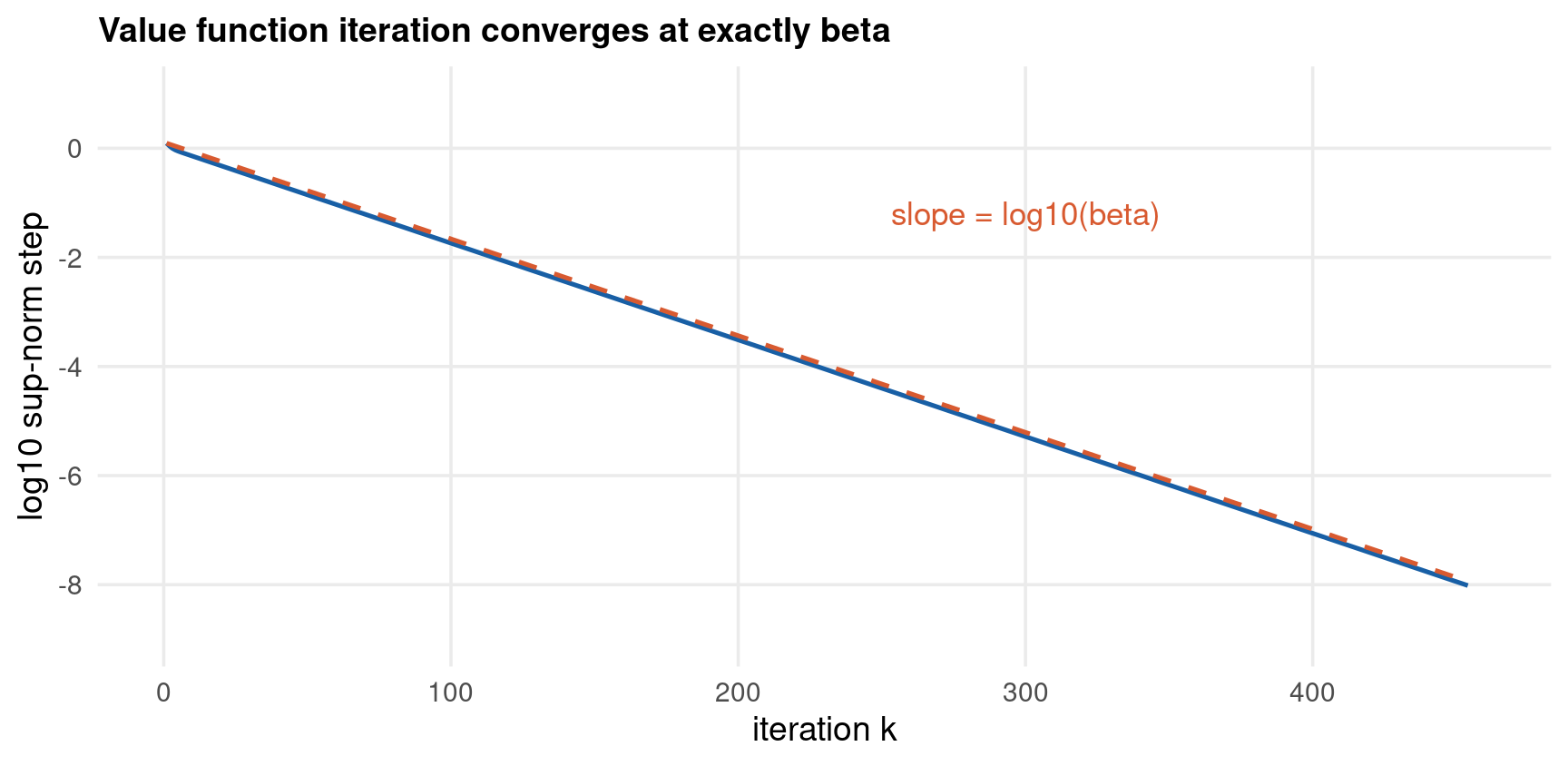
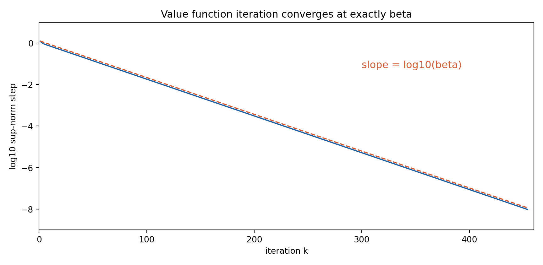
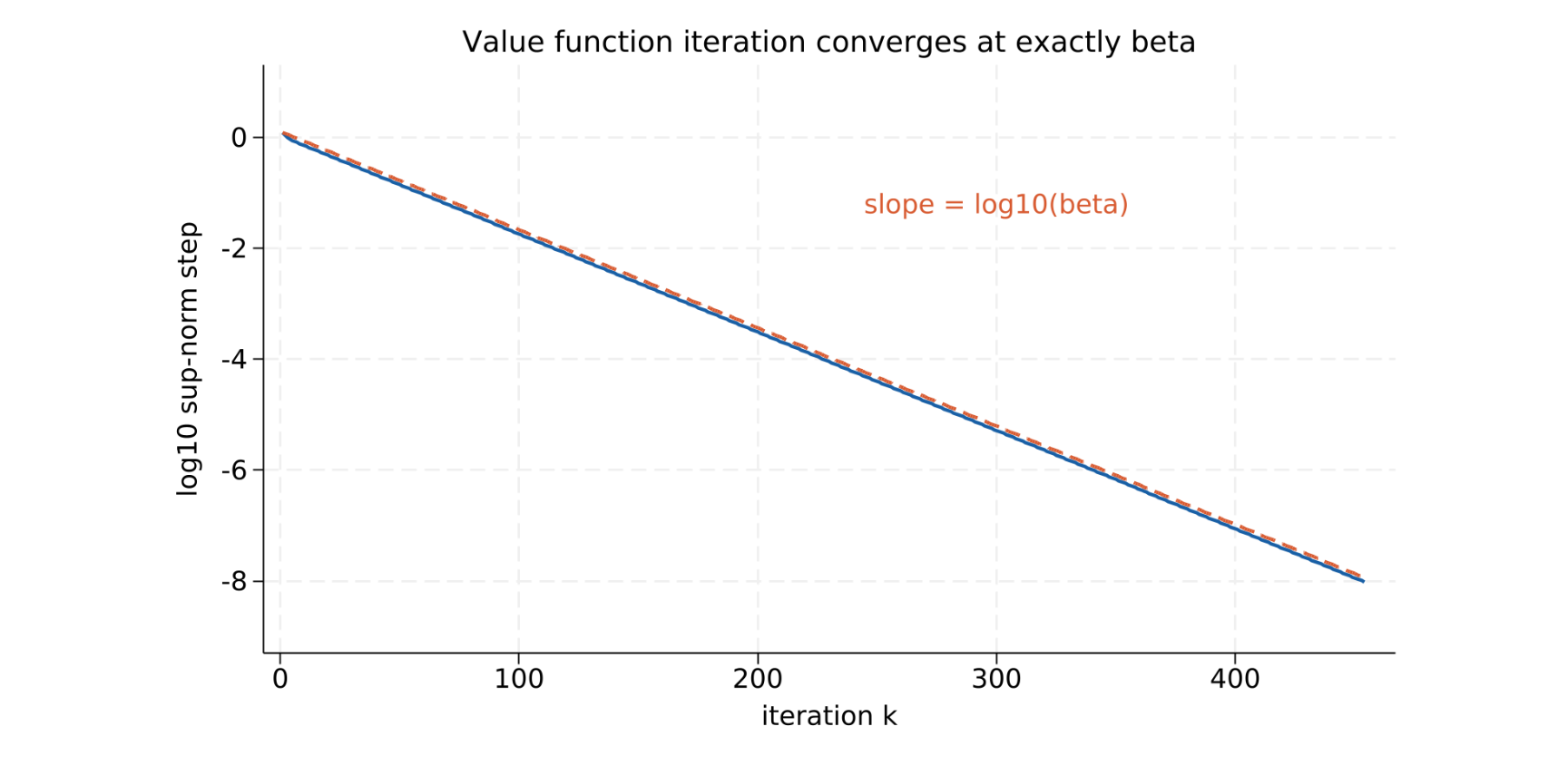
Plot the step on a log scale against the iteration number and you get a straight line. That line is the contraction property, made visible.
Its slope is \(\log_{10}\beta = -0.0177\): every iteration removes a fixed fraction of the remaining error, never a fixed amount. The line is featureless — no acceleration, no plateau, no reward for a better starting guess beyond a shift of the intercept.
The reference line drawn on each figure is the theoretical rate anchored at the first step. The computed path lies on top of it for the whole run, which is the point: this is not an algorithm that can be tuned into converging faster. It can only be replaced, which is Part 4.
a straight line in \(k\) with slope \(\log_{10}\beta\). Inverting it gives the iteration count for a target tolerance,
\[
k \;\approx\; \frac{\log_{10}(\texttt{tol}) - \log_{10}\|V_1 - V_0\|}{\log_{10}\beta}
\]
which for \(\texttt{tol} = 10^{-8}\), \(\beta = 0.96\) and a first step of order one predicts about \(460\) iterations — against the \(454\) actually taken.
Code
library(ggplot2)alpha <-0.36beta <-0.96n <-250k <-seq(0.05, 0.50, length.out = n)U <-matrix(-Inf, n, n)for (i in1:n) { cons <- k[i]^alpha - k U[i, cons >0] <-log(cons[cons >0])}V <-rep(0, n)steps <-numeric(0)for (it in1:5000) { V_new <-apply(U + beta *matrix(V, n, n, byrow =TRUE), 1, max) steps <-c(steps, max(abs(V_new - V))) V <- V_newif (steps[it] <1e-8) break}conv <-data.frame(iter =seq_along(steps),logd =log10(steps),rate =log10(steps[1]) + (seq_along(steps) -1) *log10(beta))ggplot(conv) +aes(x = iter, y = logd) +geom_line(colour ="#185FA5", linewidth =0.9) +geom_line(aes(y = rate), colour ="#D85A30",linetype ="dashed", linewidth =0.9) +annotate("text", x =300, y =-1.2, label ="slope = log10(beta)",colour ="#D85A30", size =4.6) +coord_cartesian(xlim =c(0, 460), ylim =c(-9, 1)) +scale_x_continuous(breaks =seq(0, 400, 100)) +scale_y_continuous(breaks =seq(-8, 0, 2)) +labs(x ="iteration k", y ="log10 sup-norm step",title ="Value function iteration converges at exactly beta")
The inner search wastes almost all of its work. For each state it scans every candidate \(k'\) from the bottom of the grid, including many that were already known to be too small.
In this model the optimal policy is increasing in capital: a richer household saves more. So once the optimum for \(k_i\) has been found at grid index \(j^{*}(i)\), no state above \(k_i\) can optimally choose an index below it. The search for \(k_{i+1}\) can start at \(j^{*}(i)\) rather than at \(1\).
The saving is real but bounded — roughly a third of the evaluations here, \(28{,}375{,}000\) down to \(18{,}390{,}481\). The reason it is not larger is that the policy spans most of the grid anyway, so the discarded region is small.
Monotonicity of the policy is a theorem about the model, not a property of the code — it needs supermodularity of the objective. Assuming it where it does not hold silently returns a wrong answer with no error message. Verify it, or verify the answer against a naive solve, which is what the speed slide does.
What breaks monotonicity, and how to catch it
The restriction \(j \ge j^{*}(i-1)\) is only valid if the optimal policy really is non-decreasing. That follows from supermodularity of the objective in \((k, k')\), which for this model holds because
\[ \frac{\partial^{2}}{\partial k \, \partial k'} \log\big( k^{\alpha} - k' \big) \;=\; \frac{\alpha k^{\alpha-1}}{\big(k^{\alpha} - k'\big)^{2}} \;>\; 0 \]
Change the model and that sign is no longer free. Cases where it fails, all common in applied work:
Fixed adjustment costs — the choice set becomes non-convex and the policy jumps
Discrete choices alongside the continuous one — entry, exit, replacement; the value function is a maximum over branches and need not be concave
Non-convex production or occasionally-binding constraints — the objective loses supermodularity exactly where the constraint switches
The dangerous property of the monotone search is that when the assumption fails it does not error. It simply never looks below \(j^{*}(i-1)\), so if the true optimum is there, it returns the best point in a region that excludes the answer. The result is a plausible, converged, wrong policy.
How to catch it. Solve once with the naive full search on a coarse grid and compare policies point by point. That is exactly what the speed slide does, and why its last column — the maximum difference between the naive and the accelerated value functions — is the column that matters most. It reads \(0.0\) here, to the last representable bit, which is the licence to use the fast version everywhere else.
Let \(j^{*}(i)\) be the index chosen at state \(i\):
Monotonicity says where to start the search. Concavity says when to stop it, and it is by far the bigger win.
The objective \(U_{ij} + \beta V(k_j)\) is concave in \(j\): it rises to a single peak and then falls. So the first time the value decreases as \(j\) increases, the peak has been passed and every remaining candidate is worse. Break out of the loop immediately.
Combined with monotonicity the effect is dramatic — evaluations fall from \(28{,}375{,}000\) to \(281{,}770\), a reduction of about \(100\) times. Each state now costs a handful of evaluations instead of a full scan, and the total work per sweep becomes roughly linear in \(n\) rather than quadratic.
The answer is identical — the speed slide confirms it to the last bit
It relies on genuine concavity; a spline interpolant with a spurious bump breaks it
It is a local rule, so it finds a local peak — which is the global one only if concavity really holds
Write the inner objective at state \(i\) as
\[
g_i(j) \;=\; U_{ij} + \beta V(k_j)
\]
Concavity of \(\log(\cdot)\) and of \(V\) makes \(g_i\) concave in \(j\), so its increments are decreasing:
All three variants solve the same problem to the same tolerance. Two columns tell different stories, and confusing them is the trap.
Evaluations is the algorithmic measure — deterministic, reproducible, and identical in all three languages: \(28{,}375{,}000\), \(18{,}390{,}481\), \(281{,}770\).
Seconds is the implementation measure, and it does not track evaluations at all. In R the naive sweep is a single vectorised apply over a matrix, while the monotone variant is an explicit double loop — so R runs \(35\%\)fewer evaluations more slowly. Python needs numba on the looped variants for the same reason; Mata, being compiled, does not.
The final column is the one that licenses the other two: the three value functions agree exactly, to the last representable bit.
Code
alpha <-0.36beta <-0.96n <-250k <-seq(0.05, 0.50, length.out = n)U <-matrix(-Inf, n, n)for (i in1:n) { cons <- k[i]^alpha - k U[i, cons >0] <-log(cons[cons >0])}# Naive: full vectorised scan over every candidatevfi_naive <-function() { V <-rep(0, n); ev <-0for (it in1:5000) { V_new <-apply(U + beta *matrix(V, n, n, byrow =TRUE), 1, max) ev <- ev + n * n step <-max(abs(V_new - V)) V <- V_newif (step <1e-8) break }list(V = V, it = it, ev = ev)}# Monotone starts at the previous state's optimum; concave also breaks earlyvfi_loop <-function(use_concavity) { V <-rep(0, n); ev <-0for (it in1:5000) { V_new <-numeric(n) lo <-1for (i in1:n) { best <--Inf bj <- lofor (j in lo:n) { v <- U[i, j] + beta * V[j] ev <- ev +1if (v > best) { best <- v bj <- j } elseif (use_concavity) break } V_new[i] <- best lo <- bj } step <-max(abs(V_new - V)) V <- V_newif (step <1e-8) break }list(V = V, it = it, ev = ev)}t1 <-system.time(a <-vfi_naive())[["elapsed"]]t2 <-system.time(b <-vfi_loop(FALSE))[["elapsed"]]t3 <-system.time(d <-vfi_loop(TRUE))[["elapsed"]]cat(sprintf("%-20s %6s %13s %9s %14s\n","method", "iters", "evaluations", "seconds", "max|V - V_naive|"))cat(sprintf("%-20s %6d %13d %9.2f %14.1e\n", "naive", a$it, a$ev, t1, 0))cat(sprintf("%-20s %6d %13d %9.2f %14.1e\n", "monotone", b$it, b$ev, t2,max(abs(b$V - a$V))))cat(sprintf("%-20s %6d %13d %9.2f %14.1e\n", "mono+concave", d$it, d$ev, t3,max(abs(d$V - a$V))))
method iters evaluations seconds max|V - V_naive|
naive 454 28375000 0.39 0.0e+00
monotone 454 18390481 4.26 0.0e+00
mono+concave 454 281770 0.09 0.0e+00
Code
import timeimport numpy as npfrom numba import njitalpha, beta, n =0.36, 0.96, 250k = np.linspace(0.05, 0.50, n)cons = k[:, None]**alpha - k[None, :]U = np.where(cons >0, np.log(np.where(cons >0, cons, 1.0)), -np.inf)# Naive: full vectorised scan over every candidatedef vfi_naive(): V = np.zeros(n); ev =0for it inrange(1, 5001): V_new = (U + beta * V[None, :]).max(axis=1) ev += n * n step = np.abs(V_new - V).max() V = V_newif step <1e-8:breakreturn V, it, ev# Monotone starts at the previous state's optimum; concave also breaks early@njitdef vfi_loop(U, beta, n, use_concavity): V = np.zeros(n); ev =0for it inrange(1, 5001): V_new = np.zeros(n) lo =0for i inrange(n): best =-1e300 bj = lofor j inrange(lo, n): v = U[i, j] + beta * V[j] ev +=1if v > best: best = v bj = jelif use_concavity:break V_new[i] = best lo = bj step = np.abs(V_new - V).max() V = V_newif step <1e-8:breakreturn V, it, ev# Compile before timing. The result must be assigned: a bare call in a knitr# Python chunk has its return value auto-printed into the slide.warm = vfi_loop(U, beta, n, False)warm = vfi_loop(U, beta, n, True)t0 = time.time(); Va, ita, eva = vfi_naive(); t1 = time.time() - t0t0 = time.time(); Vb, itb, evb = vfi_loop(U, beta, n, False); t2 = time.time() - t0t0 = time.time(); Vd, itd, evd = vfi_loop(U, beta, n, True); t3 = time.time() - t0rows = [("naive", ita, eva, t1, 0.0), ("monotone", itb, evb, t2, np.abs(Vb - Va).max()), ("mono+concave", itd, evd, t3, np.abs(Vd - Va).max())]out ="%-20s%6s%13s%9s%14s\n"% ("method", "iters", "evaluations","seconds", "max|V - V_naive|")out +="\n".join("%-20s%6d%13d%9.2f%14.1e"% r for r in rows)import sys; nw = sys.stdout.write(out +"\n"); sys.stdout.flush()
Three separate costs, routinely conflated into one complaint that “VFI is slow”.
The iteration count is fixed by \(\beta\). At \(\beta = 0.96\) and a tolerance of \(10^{-8}\) it is \(454\), whatever the grid, the language, or the tricks. At \(\beta = 0.99\) it is roughly four times that. Monotonicity and concavity make each sweep cheaper; they do not remove a single sweep.
The sweep cost is \(\mathcal{O}(n^2)\) and can be made \(\mathcal{O}(n)\). That is what the previous two slides bought — a factor of about \(100\) here, growing with \(n\).
The implementation constant can swamp both. The speed table shows R running fewer evaluations more slowly, because a vectorised sweep and an interpreted double loop differ by two orders of magnitude in cost per evaluation.
The order of operations that follows from this: get the algorithm right, then get the sweep cost down, and only then argue about languages. Reaching for a faster language to fix a \(\beta\)-driven iteration count is solving the wrong problem — Part 4 solves the right one.
Total work is the product of three factors that people optimise in the wrong order:
\[
\text{time}
\;\approx\;
\underbrace{\frac{\log(\texttt{tol})}{\log \beta}}_{\text{sweeps}}
\;\times\;
\underbrace{c \cdot n^{\,p}}_{\text{cost per sweep}}
\;\times\;
\underbrace{\tau}_{\text{cost per evaluation}}
\]
with \(p = 2\) for a naive scan and \(p = 1\) once monotonicity and concavity are used. Only the middle factor responds to algorithmic effort, and only the last responds to a change of language.
For a stochastic model with \(n_z\) shock states the middle factor becomes \(\mathcal{O}(n^{p} n_z^{2})\), since each state’s continuation value is itself an expectation over \(n_z\) outcomes. That extra factor, not the grid, is what makes Part 5 noticeably slower than Part 3.
The way out is to attack the first factor. Policy iteration replaces \(\log(\texttt{tol})/\log\beta\) sweeps with a handful of linear solves; the endogenous grid method removes the inner maximisation altogether. Both are Part 4.
Part 3 ended at a hard limit: value function iteration converges at \(\beta\) and nothing makes it faster. The way past it is to stop iterating on \(T\).
The observation is the one from Part 1’s popup. With the policy held fixed there is no maximum left, so the Bellman equation becomes linear — and a linear equation is solved, not iterated. Alternate two steps:
Evaluation — given a policy \(\sigma\), solve \(V_\sigma = (I - \beta Q_\sigma)^{-1} u_\sigma\) exactly
Improvement — given \(V_\sigma\), take the greedy policy it implies
Stop when the policy stops changing. On the Part 3 model this takes 9 iterations instead of \(454\), and lands on exactly the same policy at all \(250\) grid points.
The catch is the price of “exactly”. Each evaluation is a dense \(n \times n\) linear solve, costing \(\mathcal{O}(n^3)\). At \(n = 250\) that is already slower in wall-clock terms than the whole of Howard’s method below, and at the grid sizes of Parts 6–7 it is out of the question.
Fix a policy \(\sigma : \mathcal{K} \to \mathcal{K}\) and let \(Q_\sigma\) be the \(n \times n\) matrix it induces, with \([Q_\sigma]_{ij} = 1\) when \(\sigma(k_i) = k_j\) and zero otherwise. Write \(u_\sigma\) for the vector of payoffs under \(\sigma\). The value of following \(\sigma\) forever solves
The inverse exists because \(\beta < 1\) and \(Q_\sigma\) is stochastic, so \(\beta Q_\sigma\) has spectral radius \(\beta < 1\) — the contraction property of Part 1 in linear-algebra clothing. Improvement then takes
Policy iteration terminates finitely: there are finitely many policies, each step weakly improves \(V\), and no policy can repeat. That is a strictly stronger guarantee than value function iteration’s, which converges only in the limit.
Policy iteration is cheap in iterations and expensive in each one. Value function iteration is the opposite. Howard’s modified policy iteration sits between them, and in practice beats both.
The trick: do not solve\(V_\sigma = u_\sigma + \beta Q_\sigma V_\sigma\); just apply it \(m\) times. Each application costs \(\mathcal{O}(n)\) because the policy is fixed and there is no maximum to take — it is a lookup and a multiply, not a search.
So one Howard iteration costs one expensive \(\mathcal{O}(n^2)\) greedy step plus \(m\) cheap \(\mathcal{O}(n)\) ones. With \(m = 20\) the Part 3 model converges in 27 iterations rather than \(454\), with no linear solve anywhere.
\(m = 1\) recovers value function iteration
\(m \to \infty\) recovers policy iteration
\(m\) between \(20\) and \(50\) is the usual sweet spot, and the answer does not depend on it
Choosing m
\(m\) interpolates between the two extremes, and both ends are exact statements rather than approximations. At \(m = 1\) the partial evaluation is one application of \(T\) under the greedy policy, so Howard reduces to value function iteration and takes the same \(454\) iterations. As \(m\) grows the partial evaluation converges to the exact solve, and Howard becomes policy iteration.
In between, the arithmetic is simple. One iteration costs
so while \(m \ll n\) the extra evaluations are nearly free relative to the greedy step, and each one advances \(V\) further. That is why raising \(m\) from \(1\) to \(20\) cuts the iteration count by a factor of roughly \(17\) at almost no extra cost per iteration — and why raising it from \(20\) to \(200\) buys much less, because by then the \(m \cdot n\) term is no longer negligible and the policy has usually stopped changing anyway.
Two practical points:
The answer does not depend on \(m\). Only the path to it does. Any \(m \ge 1\) converges to the same fixed point, which is worth verifying once on a small problem
The greedy step is the expensive one, so the right instinct is to make \(m\) large enough that greedy steps become rare — not to tune \(m\) finely
Anything in \([20, 50]\) is a reasonable default. This deck uses \(20\).
One Howard iteration, starting from \(V_k\). First the expensive step:
so for \(m \ll n\) a Howard iteration costs barely more than a VFI iteration while advancing much further. Convergence is still monotone and still to the unique fixed point; only the number of expensive steps falls.
Everything so far iterates on the value function. But the object anyone actually wants is the policy, and the policy has its own fixed-point equation — the Euler equation.
Time iteration turns it into an operator. Given a guess at next period’s consumption function, the Euler equation pins down today’s consumption at each state, and that defines a new function. Iterate to a fixed point.
Two things change, both for the better:
No maximisation. The inner problem is a root, not a max — one equation, one unknown, and the objective is monotone, so a bisection cannot fail
No grid restriction on the choice. Consumption is solved as a real number, so the policy is not confined to grid points — which is where the accuracy comes from
On the Part 3 model this converges in 17 iterations, and the policy is accurate to \(5.9 \times 10^{-7}\) against the \(1.19 \times 10^{-3}\) of every discrete-choice method on the same grid.
The measured contraction rate here is about \(0.35\), not \(\beta = 0.96\) — close to \(\alpha\beta = 0.3456\). That is a property of this model rather than a theorem to carry elsewhere, so the code tab reports the rate instead of assuming it.
The Euler equation for the Part 3 model, with \(u'(c) = 1/c\) and \(f'(k) = \alpha k^{\alpha-1}\) under full depreciation, is
A fixed point \(C = KC\) is the optimal consumption function. The left-hand side falls in \(c\) and the right-hand side rises in \(c\), so the root is unique and bisection is guaranteed to find it — no derivative, no failure mode, no starting value to tune.
Time iteration is then
\[
C_{j+1} \;=\; K C_{j}
\]
stopped when \(\|C_{j+1} - C_j\|_\infty\) falls below tolerance. Each step needs one interpolation of \(C_j\) and one bisection per grid point.
Carroll’s (2006) observation is that even the bisection is unnecessary. The root-finding exists only because we insist on fixing \(k\)today and solving for \(c\). Turn it around.
Fix \(k'\) instead. Then the right-hand side of the Euler equation is a number you can simply evaluate — no unknown appears inside \(C(\cdot)\) — so today’s consumption follows by inverting \(u'\). The budget constraint then says which \(k\) that pair belongs to.
The grid of \(k\) values you end up with is not chosen in advance; it is generated by the solution. Hence “endogenous grid”.
Put an exogenous grid on \(k'\), tomorrow’s capital
Evaluate the Euler right-hand side — nothing to solve
Invert marginal utility to get today’s \(c\)
Recover today’s \(k\) from the budget constraint
Interpolate back onto the exogenous grid for the next pass
Same \(17\) iterations as time iteration, and the cheapest iteration in the deck.
EGM is faster but not more accurate — why
On this model EGM reaches \(1.32 \times 10^{-5}\) while time iteration reaches \(5.91 \times 10^{-7}\) — the same number of iterations, but EGM is about twenty times less accurate. That is not a bug, and it is worth understanding before trusting either number elsewhere.
The two methods make different approximations:
Time iteration solves the Euler equation exactly at each exogenous grid point. Its only error is interpolating \(C\) when the right-hand side is evaluated off-grid.
EGM makes no error solving the Euler equation — there is nothing to solve — but it produces the policy on an endogenous grid and must interpolate it back onto the exogenous one, every iteration.
So EGM trades a solving error for a resampling error, and here the resampling error is larger. The two policies differ by \(1.26 \times 10^{-5}\), essentially all of it EGM’s interpolation.
What EGM buys is speed, and the margin is not small: with no bisection, an iteration is a handful of vectorised operations. In the horse race it is the fastest method in all three languages.
Two practical consequences. If accuracy per grid point is what matters and the model is cheap, time iteration is a perfectly good choice. And EGM’s accuracy is recovered simply by using more grid points — which is affordable precisely because each iteration is so cheap. That is the trade the literature has settled on, and it is why EGM dominates the heterogeneous-agent work of Parts 6 and 7, where the household problem is solved thousands of times inside an outer loop.
Take the exogenous grid to be over tomorrow’s capital, \(k'_j\). Given a guess \(C\) for the consumption function, define for each \(j\)
Both operators on the Part 3 model, from the same starting guess \(C_0(k) = \tfrac{1}{2} k^{\alpha}\).
The bisection is written out by hand and vectorised over states, with a fixed \(60\) steps, rather than calling each language’s root-finder. That is deliberate: \(60\) bisections on this bracket is already below machine precision, and using an identical algorithm everywhere means the three tabs agree to the digit rather than to whatever their respective solvers happen to do.
Both converge in 17 iterations
Time iteration reaches \(5.9067 \times 10^{-7}\), EGM \(1.3188 \times 10^{-5}\)
The two policies differ by \(1.2597 \times 10^{-5}\) — the resampling error discussed in the popup
Code
alpha <-0.36beta <-0.96n <-250k <-seq(0.05, 0.50, length.out = n)res <- k^alphac_exact <- (1- alpha * beta) * k^alpha# Time iteration: bisect the Euler equation, vectorised across statesC <- res *0.5for (it_ti in1:5000) { lo <-rep(1e-10, n) hi <- res - k[1]for (b in1:60) { mid <- (lo + hi) /2 kp <- res - mid cn <-approx(k, C, xout = kp, rule =2)$y g <-1/ mid - beta * (1/ cn) * alpha * kp^(alpha -1) lo <-ifelse(g >0, mid, lo) hi <-ifelse(g >0, hi, mid) } C_new <- (lo + hi) /2 gap <-max(abs(C_new - C)) C <- C_newif (gap <1e-8) break}C_ti <- C# EGM: no root-finding at allC <- res *0.5rate <-0for (it_egm in1:5000) { c_today <- C / (beta * alpha * k^(alpha -1)) k_endo <- (c_today + k)^(1/ alpha) C_new <-approx(k_endo, c_today, xout = k, rule =2)$y gap_new <-max(abs(C_new - C))if (it_egm >1) rate <- gap_new / gap gap <- gap_new C <- C_newif (gap <1e-8) break}C_egm <- Ccat(sprintf("time iteration : %2d iterations, max|c - c_exact| = %11.4e\n", it_ti, max(abs(C_ti - c_exact))))cat(sprintf("EGM : %2d iterations, max|c - c_exact| = %11.4e\n", it_egm, max(abs(C_egm - c_exact))))cat(sprintf("EGM vs time iteration difference = %11.4e\n",max(abs(C_ti - C_egm))))cat(sprintf("EGM measured contraction rate = %11.4f (alpha*beta = %6.4f)\n", rate, alpha * beta))
time iteration : 17 iterations, max|c - c_exact| = 5.9067e-07
Five solvers, one model, one grid, one tolerance. The table separates two things that are usually reported as one.
Iterations is about the operator. Policy iteration and Howard cut \(454\) to \(9\) and \(27\) by replacing repeated application of \(T\) with something that jumps further each time. Time iteration and EGM cut it to \(17\) by iterating on a different object altogether.
Accuracy is about the choice set, and it splits the field cleanly in two. Every discrete-choice method — VFI, policy iteration, Howard — returns exactly the same policy and exactly the same error, \(1.193 \times 10^{-3}\), because they solve the same discretised problem and differ only in how quickly they get there. The continuous-policy methods are three orders of magnitude better on the identical grid.
The two dimensions are independent, and that is the practical lesson of Part 4: Howard makes a solver fast; only a continuous choice makes it accurate. Picking a faster discrete method and reporting a tighter tolerance improves nothing that matters.
Euler-equation methods assume an interior optimum and fail silently
The last row is the one that catches people. EGM and time iteration are built on a first-order condition holding with equality. Where a borrowing constraint binds it does not, and the method returns a plausible-looking wrong answer with no warning. Part 6 handles this explicitly — the constrained region is imposed, not solved.
Per iteration, with \(n\) grid points and \(b\) bisection steps:
Multiply by the iteration counts measured above — \(454\), \(27\), \(9\), \(17\), \(17\) — to get total cost. The ranking then changes with \(n\): policy iteration’s \(n^3\) overtakes everything as the grid grows, while EGM’s \(\mathcal{O}(n)\) per iteration together with a small iteration count makes it the only one of the five that scales comfortably into the outer loops of Parts 6 and 7.
Accuracy does not follow this ordering. On a fixed grid,
Adding a productivity shock looks like adding one more grid. It is not, and the difference shows up in three places.
The expectation is now real work. Every candidate choice needs a sum over \(n_z\) future states, so a sweep costs \(\mathcal{O}(n_k \, n_z^{2})\) rather than \(\mathcal{O}(n_k)\). The transition matrix from Part 2 finally earns its keep.
Cash-on-hand becomes the natural state. With \(\delta < 1\) the resource constraint \(m = e^{z}k^{\alpha} + (1-\delta)k\) cannot be inverted for \(k\) in closed form. Carrying \(m\) as the state instead of \(k\) keeps EGM free of root-finding — the same trick Part 6 uses for assets.
The steady state moves. Under uncertainty the model does not settle at the deterministic \(k^{*} = 5.446807\). Precautionary saving and the curvature of the return push the ergodic mean above it, and the simulation slide measures by how much.
This is the deck’s model and calibration slide — the role the standard running order gives to the DGP. There is nothing to estimate; the parameters are read from ../data/ndp-calib.csv so that all three languages provably solve the same model.
Why cash-on-hand, and not capital, is the state
In Part 4 the endogenous grid method worked because the budget constraint could be inverted in closed form. With full depreciation, \(k^{\alpha} = c + k'\) gives \(k\) directly:
\[ k \;=\; \big( c + k' \big)^{1/\alpha} \]
Set \(\delta < 1\) and that step dies. The constraint becomes
\[ e^{z} k^{\alpha} + (1-\delta) k \;=\; c + k' \]
which is a sum of a power and a linear term — not invertible for \(k\) by any rearrangement. Recovering the endogenous grid would need a root-find at every point, which is precisely the cost EGM exists to avoid.
The repair is to stop carrying \(k\) as the state and carry cash-on-hand instead:
\[ m \;\equiv\; e^{z} k^{\alpha} + (1-\delta)k \qquad\Longrightarrow\qquad m \;=\; c + k' \]
Now the endogenous step is a single addition. Given a savings level \(k'\) and the consumption \(c\) that the Euler equation implies, the cash-on-hand at which that pair is optimal is just their sum. No inversion, no solving.
The cost is one extra evaluation: to use the policy at a particular \((k, z)\) you first compute \(m\) from \(k\), which is the easy direction. The code tabs do exactly that in polc().
This is not a trick special to the growth model. Part 6’s household holds assets rather than capital and faces exactly the same structure, with \(m = (1+r)a + w \ell\); the state there is again cash-on-hand, and the same EGM step carries over unchanged. It is the standard formulation in the heterogeneous-agent literature for this reason.
Part 4’s endogenous grid method, now with a shock. The exogenous grid is over \(k'\) (savings); the endogenous grid is over cash-on-hand \(m\). Nothing is solved numerically anywhere — each iteration is an expectation, an inversion of \(u'\), and an interpolation.
168 iterations to a policy change below \(10^{-9}\), identical in all three tabs
\(k^{*} = 5.446807\) recomputed from the shared calibration
The Mata interpolator clamps outside the grid, matching R’s rule = 2 and NumPy’s np.interp. Left extrapolating instead, it converges in 166 iterations — the same policy, a different count, and a parity failure that is invisible unless you check
A solved policy is a function. To see what the model does, run it: draw a productivity path, apply the policy, and watch capital.
The three tabs read the same\(11{,}000\) uniform draws from ../data/ndp-shocks.csv, so the simulated series are identical rather than merely similar — R, Python and Stata have different generators, and without a shared stream the ergodic moments would differ in the third digit for no interesting reason.
The headline is the gap between two steady states:
the deterministic \(k^{*} = 5.4468\), where the model would sit with no shocks
the ergodic mean \(6.5261\), where it actually spends its time — about \(20\%\) higher
That wedge is precautionary saving plus the curvature of the return function. It is invisible to any method that only characterises behaviour at the steady state, and it is one of the reasons a global solution is worth its cost.
Part 3 could measure accuracy because the exact answer was known. Here it is not, and that is the normal case. The Euler equation error is what replaces it.
The idea: the optimal policy satisfies the Euler equation exactly at every state. So take the computed policy, plug it in, and ask by how much does the equation fail? No exact solution required.
Reported in \(\log_{10}\) units, the number means something concrete: a value of \(-4\) says the household is making a consumption mistake of about one dollar in ten thousand. That is an economic statement, not a numerical one, which is why this is the metric that gets published.
\(-3\) — visible in aggregates; too coarse for welfare work
\(-4\) to \(-5\) — the usual standard for a published global solution
\(-6\) and below — as good as the model deserves at this grid
This solution reaches a maximum of \(-4.472\) and a mean of \(-5.387\) over the ergodic range.
Reading a log10 Euler error as money
The normalisation is what makes the number portable. Because the error is expressed relative to consumption,
a value of \(10^{-4}\) means the household’s consumption choice is off by \(0.01\%\) — one dollar in ten thousand, whatever the units of the model.
The natural next question is what that costs in welfare, and the answer is reassuring. A consumption error \(\varepsilon\) is a first-order deviation from an optimum, so by the envelope theorem the utility loss is second order:
With \(\gamma = 2\) and \(\varepsilon = 10^{-4}\) that is a welfare cost of order \(10^{-8}\) — utterly negligible. Which is exactly why \(-4\) is treated as a respectable standard rather than a worrying one.
Two cautions before quoting the number:
Maximum, not mean. The mean here is \(-5.387\) and the maximum \(-4.472\) — nearly a full decade apart. A paper that reports only the mean is reporting the easy states. The maximum is the claim a referee can check
State the region. Errors are largest where the policy is most curved, so an error computed on a narrow band around the steady state can be an order of magnitude too flattering. This deck evaluates over \(k \in [2, 12]\), which brackets the simulated range
The second point is the one that quietly inflates published accuracy figures, because the evaluation region is so often left unstated.
Given a computed policy \(\hat{c}(k,z)\) with \(k' = m - \hat c(k,z)\), define the consumption the Euler equation would have implied:
reported as \(\log_{10} \mathcal{E}\). The normalisation by \(\hat c\) is what makes it interpretable: \(\mathcal{E} = 10^{-4}\) is a consumption error of \(0.01\%\), independent of units.
Two reporting conventions matter, and papers differ on them. The maximum over the evaluated region is the honest headline; the mean flatters. And the region matters — errors are largest where the constraint is near binding, so an error computed only near the steady state can be an order of magnitude too optimistic. Both are reported here, over \(k \in [2, 12]\).
Code
ktest <-seq(2, 12, length.out =400)ee <-matrix(0, length(ktest), nz)for (iz in1:nz) { c_hat <-polc(ktest, iz) kprime <-Mk(ktest, z[iz]) - c_hat rhs <-rep(0, length(ktest))for (jz in1:nz) { rhs <- rhs + Pi[iz, jz] *polc(kprime, jz)^(-gamma) *Rk(kprime, z[jz]) } c_tilde <- (beta * rhs)^(-1/ gamma) ee[, iz] <-abs(1- c_tilde / c_hat)}cat(sprintf("evaluated on k in [2, 12] x %d productivity states\n", nz))cat(sprintf("max log10 Euler error : %8.3f\n", log10(max(ee))))cat(sprintf("mean log10 Euler error : %8.3f\n", mean(log10(ee))))cat(sprintf("worst state is z = %9.4f\n", z[which.max(apply(ee, 2, max))]))
evaluated on k in [2, 12] x 7 productivity states
max  log10 Euler error :   -4.472
mean log10 Euler error :   -5.387
worst state is z =   -0.1873
Code
ktest = np.linspace(2, 12, 400)ee = np.zeros((len(ktest), nz))for iz inrange(nz): c_hat = polc(ktest, iz) kprime = Mk(ktest, z[iz]) - c_hat rhs = np.zeros(len(ktest))for jz inrange(nz): rhs += Pi[iz, jz] * polc(kprime, jz)**(-gamma) * Rk(kprime, z[jz]) c_tilde = (beta * rhs)**(-1/ gamma) ee[:, iz] = np.abs(1- c_tilde / c_hat)out = (f"evaluated on k in [2, 12] x {nz:d} productivity states\n"f"max log10 Euler error : {np.log10(ee.max()):8.3f}\n"f"mean log10 Euler error : {np.log10(ee).mean():8.3f}\n"f"worst state is z = {z[ee.max(axis=0).argmax()]:9.4f}")import sys; nw = sys.stdout.write(out +"\n"); sys.stdout.flush()
evaluated on k in [2, 12] x 7 productivity states
max log10 Euler error : -4.472
mean log10 Euler error : -5.387
worst state is z = -0.1873
Solve the same model on grids of \(25\), \(50\), \(100\) and \(200\) points and watch the Euler error. Each doubling improves \(\log_{10}\) accuracy by about \(0.6\) — which is \(\log_{10} 4\), so the error falls by a factor of four when the spacing halves.
\[
\mathcal{E} \;=\; \mathcal{O}(h^{2})
\]
That is the second-order convergence Part 4 claimed for a continuous choice set, now measured rather than asserted. A discrete choice set would give \(\mathcal{O}(h)\) — a factor of two per doubling, or \(0.3\) in \(\log_{10}\) — and you can tell which regime you are in from the table alone.
This is the single most useful diagnostic in the deck, because it needs no exact solution and no theory. Solve on two grids. If the error does not fall at the rate your method promises, something is wrong — and it is usually an interpolation or an unhandled constraint, not the tolerance.
------------------------------------------------- mata (type end to exit) ----------------------------------------------
: real colvector interpA(real colvector xg, real colvector yg,
> real colvector xq) {
> real colvector yq
> real scalar n, m, i, j
> n = rows(xg)
> m = rows(xq)
> yq = J(m, 1, 0)
> j = 1
> for (i = 1; i <= m; i++) {
> if (xq[i] <= xg[1]) {
> yq[i] = yg[1]
> }
> else if (xq[i] >= xg[n]) {
> yq[i] = yg[n]
> }
> else {
> while (j < n - 1 & xg[j+1] < xq[i]) j++
> yq[i] = yg[j] + (yg[j+1] - yg[j]) *
> (xq[i] - xg[j]) / (xg[j+1] - xg[j])
> }
> }
> return(yq)
> }
: real colvector polc(real matrix m_endo, real matrix c_endo, real colvector kk,
> real scalar iz, real colvector z, real scalar alpha,
> real scalar delta, real scalar kmin) {
> real colvector cc
> real scalar i, mm
> cc = J(rows(kk), 1, 0)
> for (i = 1; i <= rows(kk); i++) {
> mm = exp(z[iz])*kk[i]^alpha + (1-delta)*kk[i]
> cc[i] = min((interpA(m_endo[,iz], c_endo[,iz], mm)[1], mm - kmin))
> }
> return(cc)
> }
: nz = 7
: beta = st_numscalar("beta")
: gamma = st_numscalar("gamma")
: alpha = st_numscalar("alpha")
: delta = st_numscalar("delta")
: Pi = rowshape(st_data(., "p"), nz)
: z = rowshape(st_data(., "z_i"), nz)[,1]
: kmin = 0.5
: kmax = 20
: ktest = 2 :+ (0..399)' :* (10/399)
:
: grids = (25, 50, 100, 200)
: printf("%6s %14s %15s %10s\n",
> "points", "max log10 EE", "mean log10 EE", "gain")
points max log10 EE mean log10 EE gain
: prev = .
: for (q = 1; q <= 4; q++) {
> na = grids[q]
> s = (0..na-1)' :/ (na-1)
> kpn = kmin :+ (kmax-kmin) :* s:^2
> me = J(na, nz, 0)
> ce = J(na, nz, 0)
> for (iz = 1; iz <= nz; iz++) {
> Mz = exp(z[iz]) :* kpn:^alpha + (1-delta) :* kpn
> ce[,iz] = 0.3 :* Mz
> me[,iz] = ce[,iz] + kpn
> }
> for (it = 1; it <= 3000; it++) {
> cn2 = J(na, nz, 0)
> mn2 = J(na, nz, 0)
> for (iz = 1; iz <= nz; iz++) {
> rhs = J(na, 1, 0)
> for (jz = 1; jz <= nz; jz++) {
> mn = exp(z[jz]) :* kpn:^alpha + (1-delta) :* kpn
> Rnext = alpha*exp(z[jz]) :* kpn:^(alpha-1) :+ (1-delta)
> rhs = rhs + Pi[iz,jz] :*
> interpA(me[,jz], ce[,jz], mn):^(-gamma) :* Rnext
> }
> cn2[,iz] = (beta :* rhs):^(-1/gamma)
> mn2[,iz] = cn2[,iz] + kpn
> }
> gap = max(abs(cn2 - ce))
> ce = cn2
> me = mn2
> if (gap < 1e-9) break
> }
> ee = J(400, nz, 0)
> for (iz = 1; iz <= nz; iz++) {
> ch = polc(me, ce, ktest, iz, z, alpha, delta, kmin)
> kpp = exp(z[iz]) :* ktest:^alpha + (1-delta) :* ktest - ch
> rhs = J(400, 1, 0)
> for (jz = 1; jz <= nz; jz++) {
> cn = polc(me, ce, kpp, jz, z, alpha, delta, kmin)
> Rnext = alpha*exp(z[jz]) :* kpp:^(alpha-1) :+ (1-delta)
> rhs = rhs + Pi[iz,jz] :* cn:^(-gamma) :* Rnext
> }
> ee[,iz] = abs(1 :- (beta :* rhs):^(-1/gamma) :/ ch)
> }
> mx = log10(max(ee))
> mnv = mean(mean(log10(ee))')
> if (q == 1) {
> printf("%6.0f %14.3f %15.3f %10s\n", na, mx, mnv, "-")
> }
> else {
> printf("%6.0f %14.3f %15.3f %10.3f\n", na, mx, mnv, prev - mx)
> }
> prev = mx
> }
    25         -2.705          -3.529          -
    50         -3.302          -4.152      0.597
   100         -3.927          -4.783      0.625
   200         -4.472          -5.387      0.545
: end
------------------------------------------------------------------------------------------------------------------------
Code
# The convergence table as LaTeX source, ready to paste into a paper.# Built with sprintf rather than a table package so that what is emitted is# exactly what is shown - no package defaults, no hidden formatting.cat("\\begin{tabular}{rrrr}\n")cat("\\hline\n")cat("points & $\\max \\log_{10}\\mathcal{E}$ &","$\\overline{\\log_{10}\\mathcal{E}}$ & gain \\\\\n")cat("\\hline\n")for (i inseq_len(nrow(order_tab))) {cat(sprintf("%d & %.3f & %.3f & %s \\\\\n", order_tab$points[i], order_tab$max_ee[i], order_tab$mean_ee[i],if (is.na(order_tab$gain[i])) "--"elsesprintf("%.3f", order_tab$gain[i])))}cat("\\hline\n")cat("\\end{tabular}\n")
\begin{tabular}{rrrr}
\hline
points & $\max \log_{10}\mathcal{E}$ & $\overline{\log_{10}\mathcal{E}}$ & gain \\
The gain column is the whole diagnostic: \(0.6\) per row is \(\log_{10} 4\), so the error falls fourfold when the spacing halves — second order. Report this table, not the tolerance.
Euler errors are computed on a grid the modeller chooses. The den Haan–Marcet test instead asks whether the errors behave correctly along a simulated path — that is, in the states the model actually visits.
The logic is exactly a GMM overidentification test. If the solution were exact, the realised Euler residual would be a forecast error: unpredictable given any information available at \(t\). So regress it on instruments known at \(t\) and test whether the moments are jointly zero.
Fails to reject no detectable systematic error
Rejects the residual is predictable, so the policy is wrong in a specific, findable way
On this solution the statistic is \(0.4635\) on \(3\) degrees of freedom, \(p = 0.9268\) — comfortably not rejected.
Not rejecting is weak evidence, and its power grows with the sample: a long enough simulation will reject any approximate solution, because none is exact. Report the statistic together with \(T\), and read it alongside the Euler errors rather than instead of them.
A long enough simulation rejects every solution
The test is consistent, and that is the problem. Under a fixed approximation error the sample moment \(\bar{g}\) converges to some non-zero \(g_0\) rather than to zero, so
\[ J \;=\; T \, \bar{g}' \widehat{S}^{-1} \bar{g} \;\approx\; T \cdot g_0' S^{-1} g_0 \;\longrightarrow\; \infty \]
The statistic grows linearly in \(T\). Since no numerical solution is exact, \(g_0 \neq 0\) always, and a long enough simulation therefore rejects any solution ever computed. The result here, \(J = 0.4635\) at \(T = 9999\), is a statement about this solution at this sample size — not a certificate.
Three consequences for how to use it:
Always report \(T\). A \(p\)-value without it is uninterpretable, because the alternative hypothesis is “your solver is imperfect”, which is certainly true
Use it comparatively. The informative exercise is running the same \(T\) against two solutions — two grid sizes, two methods — and seeing which rejects first. That ranks approximations, which is what you actually want to know
Read it with the Euler errors, not instead of them. The two diagnose different things: Euler errors measure the size of the mistake on a region you choose, den Haan–Marcet measures whether the mistake is systematic in the states the model visits
A solution can pass one and fail the other, and both failures are informative. Small errors that are strongly predictable point to a structural problem — an unhandled constraint, a grid that does not reach far enough — rather than to insufficient resolution.
Along the simulated path, form the realised Euler residual
The residual is a one-step-ahead forecast error, so it is serially uncorrelated under the null and no HAC correction is needed — a convenience specific to this test.
Macro-Finance Simulation solves models like this one by perturbation: take a Taylor expansion of the equilibrium conditions around the deterministic steady state and use it everywhere. It is fast, it scales to dozens of state variables, and it is what most of the DSGE literature runs.
This deck solves the same model globally: the policy is computed at every point of the state space, with no expansion point and no assumption that the economy stays near it.
The two agree where they should and diverge where they must:
At the steady state they match. The slope of the global policy in \(\log k\) is \(0.922661\) against the perturbation’s \(0.924166\) — a \(0.2\%\) difference, which is the global solution’s own grid error
Far away they do not. At half the steady-state capital and the highest productivity state the linear rule under-saves by \(9.8\%\)
The gap is asymmetric. At twice \(k^{*}\) the error is only \(0.55\%\): the policy is far more curved below the steady state than above it
That asymmetry is the general lesson. Perturbation is a local method, and its errors are largest exactly where the interesting economics is — near constraints, after large shocks, in the left tail.
Log-linearising the Euler and resource constraints around \(k^{*}\) and guessing
\[
\hat{k}' \;=\; a \, \hat{k} + b \, z ,
\qquad \hat{x} \equiv \log(x / x^{*})
\]
the coefficient \(a\) solves a quadratic whose stable root is taken. With \(y^{*} = (k^{*})^{\alpha}\), \(c^{*} = y^{*} - \delta k^{*}\), \(\varphi = \beta \alpha (k^{*})^{\alpha-1}\) and \(P = \alpha y^{*} + (1-\delta)k^{*}\),
\[
\gamma k^{*} a^{2}
\;-\; \Big[ \gamma P + \gamma k^{*} - \varphi(\alpha-1) c^{*} \Big] a
\;+\; \gamma P \;=\; 0
\]
giving \(a = 0.924166\) and \(b = 0.208481\) for this calibration. The perturbation policy is then
\[
k'_{\text{pert}}(k, z) \;=\; k^{*}
\exp\Big\{ a \log(k/k^{*}) + b \, z \Big\}
\]
which the code compares against the global policy across the state space. Second order adds curvature and shrinks the gap, but the expansion remains local — the cross-link to Macro-Finance Simulation is where that machinery lives.
perturbation a (slope in log k) : 0.924166
global a (numerical) : 0.922661
perturbation b (loading on z) : 0.208481
k / k* global k' perturbation gap %
      0.50      3.57798        3.22716      -9.81
      0.75      4.99060        4.69416      -5.94
      1.00      6.36427        6.12382      -3.78
      1.50      9.04864        8.90759      -1.56
      2.00     11.68494       11.62048      -0.55
Code
quietly import delimited "../data/ndp-calib.csv", clearscalar beta = beta[1]scalargamma = gamma[1]scalaralpha = alpha[1]scalar delta = delta[1]scalar rho = rho[1]quietly import delimited "../data/ndp-income.csv", clearmata:realcolvector interpA(realcolvector xg, realcolvector yg,realcolvector xq) {realcolvectoryqrealscalar n, m, i, j n = rows(xg)m = rows(xq)yq = J(m, 1, 0) j = 1for (i = 1; i <= m; i++) {if (xq[i] <= xg[1]) {yq[i] = yg[1] }elseif (xq[i] >= xg[n]) {yq[i] = yg[n] }else {while (j < n - 1 & xg[j+1] < xq[i]) j++yq[i] = yg[j] + (yg[j+1] - yg[j]) * (xq[i] - xg[j]) / (xg[j+1] - xg[j]) } }return(yq)} beta = st_numscalar("beta")gamma = st_numscalar("gamma")alpha = st_numscalar("alpha") delta = st_numscalar("delta") rho = st_numscalar("rho") kss = (alpha/(1/beta - 1 + delta))^(1/(1-alpha)) yss = kss^alpha css = yss - delta*kss phi = beta*alpha*kss^(alpha-1) Pc = alpha*yss + (1-delta)*kss// Stable root of the log-linearised policy A2 = gamma*kss A1 = -(gamma*Pc + gamma*kss - phi*(alpha-1)*css) A0 = gamma*Pc disc = sqrt(A1^2 - 4*A2*A0) r1 = (-A1 + disc)/(2*A2) r2 = (-A1 - disc)/(2*A2) a = abs(r1) < 1 ? r1 : r2 b = (gamma*yss*(1-rho) + phi*rho*css) / (gamma*kss*(1-rho) + gamma*(Pc - kss*a) - phi*(alpha-1)*css)// Solve the model globally so the two rules can be compared directly nz = 7 Pi = rowshape(st_data(., "p"), nz) z = rowshape(st_data(., "z_i"), nz)[,1] na = 200 kmin = 0.5 kmax = 20s = (0..na-1)' :/ (na-1) kp = kmin :+ (kmax-kmin) :* s:^2 m_endo = J(na, nz, 0) c_endo = J(na, nz, 0)for (iz = 1; iz <= nz; iz++) { Mz = exp(z[iz]) :* kp:^alpha + (1-delta) :* kp c_endo[,iz] = 0.3 :* Mz m_endo[,iz] = c_endo[,iz] + kp }for (it = 1; it <= 3000; it++) { c_new = J(na, nz, 0) m_new = J(na, nz, 0)for (iz = 1; iz <= nz; iz++) { rhs = J(na, 1, 0)for (jz = 1; jz <= nz; jz++) { m_next = exp(z[jz]) :* kp:^alpha + (1-delta) :* kp Rnext = alpha*exp(z[jz]) :* kp:^(alpha-1) :+ (1-delta) rhs = rhs + Pi[iz,jz] :* interpA(m_endo[,jz], c_endo[,jz], m_next):^(-gamma) :* Rnext } c_new[,iz] = (beta :* rhs):^(-1/gamma) m_new[,iz] = c_new[,iz] + kp } gap = max(abs(c_new - c_endo)) c_endo = c_new m_endo = m_newif (gap < 1e-9) break }// Numerical slope of the global policy in log k at (k*, z = 0) imid = (nz + 1) / 2h = 1e-4 gk = J(2, 1, 0) kq = (kss*exp(h) \ kss*exp(-h))for (q = 1; q <= 2; q++) { mm = exp(z[imid])*kq[q]^alpha + (1-delta)*kq[q]ct = min((interpA(m_endo[,imid], c_endo[,imid], mm)[1], mm - kmin)) gk[q] = mm - ct } slope = (log(gk[1]) - log(gk[2])) / (2*h) printf("perturbation a (slope in log k) : %12.6f\n", a) printf("global a (numerical) : %12.6f\n", slope) printf("perturbation b (loading on z) : %12.6f\n", b) printf("the two roots are %8.6f and %8.6f; the stable one is taken\n", r1, r2) printf("\n%10s %12s %14s %10s\n", "k / k*", "global k'", "perturbation", "gap %") frac = (0.50, 0.75, 1.00, 1.50, 2.00)for (q = 1; q <= 5; q++) { kq2 = kss * frac[q] mm = exp(z[nz])*kq2^alpha + (1-delta)*kq2ct = min((interpA(m_endo[,nz], c_endo[,nz], mm)[1], mm - kmin)) gkq = mm - ct pkq = kss * exp(a*log(kq2/kss) + b*z[nz]) printf("%10.2f %12.5f %14.5f %10.2f\n", frac[q], gkq, pkq, 100*(pkq/gkq - 1)) }end
------------------------------------------------- mata (type end to exit) ----------------------------------------------
: real colvector interpA(real colvector xg, real colvector yg,
>                        real colvector xq) {
>     real colvector yq
>     real scalar n, m, i, j
>     n  = rows(xg)
>     m  = rows(xq)
>     yq = J(m, 1, 0)
>     j  = 1
>     for (i = 1; i <= m; i++) {
>         if (xq[i] <= xg[1]) {
>             yq[i] = yg[1]
>         }
>         else if (xq[i] >= xg[n]) {
>             yq[i] = yg[n]
>         }
>         else {
>             while (j < n - 1 & xg[j+1] < xq[i]) j++
>             yq[i] = yg[j] + (yg[j+1] - yg[j]) *
>                             (xq[i] - xg[j]) / (xg[j+1] - xg[j])
>         }
>     }
>     return(yq)
> }

:     beta  = st_numscalar("beta")

:     gamma = st_numscalar("gamma")

:     alpha = st_numscalar("alpha")

:     delta = st_numscalar("delta")

:     rho   = st_numscalar("rho")

:
:     kss = (alpha/(1/beta - 1 + delta))^(1/(1-alpha))

:     yss = kss^alpha

:     css = yss - delta*kss

:     phi = beta*alpha*kss^(alpha-1)

:     Pc  = alpha*yss + (1-delta)*kss

:
:     // Stable root of the log-linearised policy
:     A2 = gamma*kss

:     A1 = -(gamma*Pc + gamma*kss - phi*(alpha-1)*css)

:     A0 = gamma*Pc

:     disc = sqrt(A1^2 - 4*A2*A0)

:     r1 = (-A1 + disc)/(2*A2)

:     r2 = (-A1 - disc)/(2*A2)

:     a  = abs(r1) < 1 ? r1 : r2

:     b  = (gamma*yss*(1-rho) + phi*rho*css) /
>          (gamma*kss*(1-rho) + gamma*(Pc - kss*a) - phi*(alpha-1)*css)

:
:     // Solve the model globally so the two rules can be compared directly
:     nz = 7

:     Pi = rowshape(st_data(., "p"),   nz)

:     z  = rowshape(st_data(., "z_i"), nz)[,1]

:     na   = 200

:     kmin = 0.5

:     kmax = 20

:     s    = (0..na-1)' :/ (na-1)

:     kp   = kmin :+ (kmax-kmin) :* s:^2

:     m_endo = J(na, nz, 0)

:     c_endo = J(na, nz, 0)

:     for (iz = 1; iz <= nz; iz++) {
>         Mz = exp(z[iz]) :* kp:^alpha + (1-delta) :* kp
>         c_endo[,iz] = 0.3 :* Mz
>         m_endo[,iz] = c_endo[,iz] + kp
>     }

:     for (it = 1; it <= 3000; it++) {
>         c_new = J(na, nz, 0)
>         m_new = J(na, nz, 0)
>         for (iz = 1; iz <= nz; iz++) {
>             rhs = J(na, 1, 0)
>             for (jz = 1; jz <= nz; jz++) {
>                 m_next = exp(z[jz]) :* kp:^alpha + (1-delta) :* kp
>                 Rnext  = alpha*exp(z[jz]) :* kp:^(alpha-1) :+ (1-delta)
>                 rhs = rhs + Pi[iz,jz] :*
>                       interpA(m_endo[,jz], c_endo[,jz], m_next):^(-gamma) :* Rnext
>             }
>             c_new[,iz] = (beta :* rhs):^(-1/gamma)
>             m_new[,iz] = c_new[,iz] + kp
>         }
>         gap = max(abs(c_new - c_endo))
>         c_endo = c_new
>         m_endo = m_new
>         if (gap < 1e-9) break
>     }

:
:     // Numerical slope of the global policy in log k at (k*, z = 0)
:     imid = (nz + 1) / 2

:     h    = 1e-4

:     gk = J(2, 1, 0)

:     kq = (kss*exp(h) \ kss*exp(-h))

:     for (q = 1; q <= 2; q++) {
>         mm = exp(z[imid])*kq[q]^alpha + (1-delta)*kq[q]
>         ct = min((interpA(m_endo[,imid], c_endo[,imid], mm)[1], mm - kmin))
>         gk[q] = mm - ct
>     }

:     slope = (log(gk[1]) - log(gk[2])) / (2*h)

:
:     printf("perturbation a (slope in log k) : %12.6f\n", a)
perturbation a (slope in log k) :     0.924166

:     printf("global       a (numerical)      : %12.6f\n", slope)
global       a (numerical)      :     0.922661

:     printf("perturbation b (loading on z)   : %12.6f\n", b)
perturbation b (loading on z)   :     0.208481

:     printf("the two roots are %8.6f and %8.6f; the stable one is taken\n", r1, r2)
the two roots are 1.127142 and 0.924166; the stable one is taken

:     printf("\n%10s %12s %14s %10s\n", "k / k*", "global k'", "perturbation", "gap %")

    k / k*    global k'   perturbation      gap %

:     frac = (0.50, 0.75, 1.00, 1.50, 2.00)

:     for (q = 1; q <= 5; q++) {
>         kq2 = kss * frac[q]
>         mm  = exp(z[nz])*kq2^alpha + (1-delta)*kq2
>         ct  = min((interpA(m_endo[,nz], c_endo[,nz], mm)[1], mm - kmin))
>         gkq = mm - ct
>         pkq = kss * exp(a*log(kq2/kss) + b*z[nz])
>         printf("%10.2f %12.5f %14.5f %10.2f\n",
>                frac[q], gkq, pkq, 100*(pkq/gkq - 1))
>     }
      0.50      3.57798        3.22716      -9.81
      0.75      4.99060        4.69416      -5.94
      1.00      6.36427        6.12382      -3.78
      1.50      9.04864        8.90759      -1.56
      2.00     11.68494       11.62048      -0.55

: end
------------------------------------------------------------------------------------------------------------------------
A solved model is a claim, and these are the numbers that let a reader check it. Every one of them appears somewhere in Parts 3–5.
The grid — bounds, number of points, spacing rule. “200 points, curved, \([0.5, 20]\)”, not “a fine grid”
The discretisation — method, number of states, and the implied\(\rho\) and \(\sigma\), not just the targets
The solver and its tolerance — and the tolerance’s implied error bound, not the tolerance alone
Euler errors — maximum and mean, in \(\log_{10}\), with the region they were computed over
The convergence order — errors on at least two grid sizes, so the reader can see the rate
The ergodic range — where the simulation actually goes, and confirmation that the grid contains it
A simulation-based test — den Haan–Marcet or equivalent, with \(T\)
Whether the choice set was discrete — this caps accuracy at \(\mathcal{O}(h)\) and is very often left unsaid
The most common omission is the last one, and the most common overstatement is quoting a tolerance of \(10^{-10}\) as though it described the answer’s accuracy. Part 3 measured the gap on a model with a known solution: the tolerance implied \(2.3 \times 10^{-7}\) while the true error was \(1.07 \times 10^{-4}\).
Everything so far had one agent. Now there are a continuum of them, each hit by their own income shock, each saving to smooth it, and no insurance market.
The household problem barely changes: it is the consumption-savings problem of Part 5 with labour income instead of a productivity shock to capital. What changes is what we do with the answer. The object of interest is no longer the policy function but the distribution of agents across states that the policy generates — and that distribution is itself a fixed point.
The whole model turns on one inequality:
\[
a' \;\ge\; \underline{a}
\]
Without it, a household hit by bad luck simply borrows, consumption is perfectly smooth, and aggregate saving is whatever the representative agent would choose. With it, households near the constraint cannot borrow, so they must self-insure by holding a buffer of assets they would rather spend. Aggregate capital rises, and the equilibrium interest rate falls below the rate of time preference.
Everything computed in this part uses \(r = 0.037002\), the market-clearing rate found three slides on. Households take prices as given, so the household problem never needs to know where \(r\) came from — but each code tab prints the excess demand at that rate as a check that it really is the equilibrium.
\[
c + a' \;=\; (1 + r) \, a + w \, \ell \;\equiv\; m
\]
where \(\ell\) is the Part 2 productivity chain, normalised so that \(\sum_\ell \pi_\ell \, \ell = 1\) and aggregate labour supply is exactly one.
Firms are competitive with \(Y = K^{\alpha} L^{1-\alpha}\) and \(L = 1\), so prices are functions of capital alone:
\[
r \;=\; \alpha K^{\alpha - 1} - \delta,
\qquad
w \;=\; (1-\alpha) K^{\alpha}
\]
A stationary recursive competitive equilibrium is a policy \(a'(a,\ell)\), a distribution \(\mu\), and prices \((r, w)\) such that the policy is optimal, the distribution is invariant under the policy, and the asset market clears:
\[
\int a \; d\mu(a, \ell) \;=\; K
\]
The borrowing limit used here is \(\underline{a} = 0\): households may save but never borrow. That is the tightest possible constraint and the one Aiyagari’s headline results use.
Part 5’s endogenous grid method, with two changes. The return is now the fixed \(1+r\) rather than a state-dependent marginal product, and — the substantive one — the borrowing constraint must be imposed by hand.
EGM inverts a first-order condition that holds with equality. Where the constraint binds it does not hold, so no amount of iterating will produce the right answer there. The fix is the two-line rule in each tab: below the smallest endogenous cash-on-hand, the household is constrained, saves exactly \(\underline{a}\), and consumes everything else.
443 EGM iterations at \(r = 0.037002\), identical in all three tabs
25 of 840 grid states are constrained — a small corner of the state space carrying most of the model’s economics
Excess demand at this \(r\) is order \(10^{-6}\), confirming it is the market-clearing rate
Why EGM cannot find the constrained region by itself
Part 4 flagged this as the one row of the decision table that catches people. Here is the mechanism.
Every Euler-equation method starts from the first-order condition holding with equality:
That is the condition for an interior optimum. Where the borrowing constraint binds the correct condition is an inequality — the household would like to borrow, cannot, and so its marginal utility today is strictly higher than the discounted expected marginal utility tomorrow:
EGM never sees this. It fixes \(a'\) on a grid that starts at \(\underline{a}\), computes the \(c\) that would make the equality hold, and reports the cash-on-hand \(m = c + a'\) at which that is optimal. The smallest such \(m\) — call it \(m_1\) — is the level of resources at which the household is just unconstrained.
For any \(m < m_1\) the household is constrained, and EGM has simply produced no point there. Interpolating into that region is extrapolation, and it returns a smooth continuation of the unconstrained policy: a household that saves a little less, rather than one pinned at the constraint. The error is invisible — the policy still looks monotone and concave.
The repair is one line, and it is exact rather than approximate:
\[ c(m, \ell) \;=\; m - \underline{a} \qquad \text{whenever} \qquad m \;<\; m_1(\ell) \]
because a constrained household saves exactly \(\underline{a}\) and eats the rest. Note that the threshold \(m_1\) depends on \(\ell\): a household with high current income needs more resources before it stops wanting to borrow.
Skip this and the model still solves, still converges, and still produces a plausible equilibrium — with too little mass at the constraint, too little precautionary saving, and an interest rate that is too high. It is the most consequential silent error in this deck.
Code
cal <-read.csv("../data/ndp-calib.csv")inc <-read.csv("../data/ndp-income.csv")beta <- cal$beta; gamma <- cal$gamma; alpha <- cal$alphadelta <- cal$delta; nz <- cal$n_zPi <-matrix(inc$p, nz, nz, byrow =TRUE)l <- inc$l_i[seq(1, nz * nz, by = nz)]na <-120amin <-0amax <-60s <-seq(0, 1, length.out = na)agrid <- amin + (amax - amin) * s^3# heavily curved: mass sits low# The market-clearing rate, found on the equilibrium slider_eq <-0.037002Kd <- (alpha / (r_eq + delta))^(1/ (1- alpha))w <- (1- alpha) * Kd^alpham_endo <-matrix(0, na, nz)c_endo <-matrix(0, na, nz)for (i in1:nz) { c_endo[, i] <-0.3* ((1+ r_eq) * agrid + w * l[i]) m_endo[, i] <- c_endo[, i] + agrid}for (it in1:20000) { c_new <-matrix(0, na, nz) m_new <-matrix(0, na, nz)for (i in1:nz) { rhs <-rep(0, na)for (j in1:nz) { m_next <- (1+ r_eq) * agrid + w * l[j] c_next <-approx(m_endo[, j], c_endo[, j], xout = m_next, rule =2)$y# constrained: below the smallest endogenous m, save amin and eat the rest c_next <-ifelse(m_next < m_endo[1, j], m_next - amin, c_next) rhs <- rhs + Pi[i, j] * c_next^(-gamma) } c_new[, i] <- (beta * (1+ r_eq) * rhs)^(-1/ gamma) m_new[, i] <- c_new[, i] + agrid } gap <-max(abs(c_new - c_endo)) c_endo <- c_new m_endo <- m_newif (gap <1e-9) break}# Asset policy on the grid, with the same constrained ruleap <-matrix(0, na, nz)for (i in1:nz) { mm <- (1+ r_eq) * agrid + w * l[i] cc <-approx(m_endo[, i], c_endo[, i], xout = mm, rule =2)$y cc <-ifelse(mm < m_endo[1, i], mm - amin, cc) ap[, i] <-pmin(pmax(mm - cc, amin), amax)}cat(sprintf("interest rate r : %11.6f (1/beta - 1 = %.6f)\n", r_eq, 1/ beta -1))cat(sprintf("wage w : %11.6f\n", w))cat(sprintf("EGM iterations : %11d\n", it))cat(sprintf("constrained states : %d of %d\n",sum(ap <= amin +1e-12), na * nz))cat(sprintf("capital demanded at r : %11.6f\n", Kd))
interest rate r        :    0.037002   (1/beta - 1 = 0.041667)
wage w                 :    1.204319
EGM iterations         :         443
constrained states     : 25 of 840
capital demanded at r  :    5.789894
Code
import numpy as npimport pandas as pdcal = pd.read_csv("../data/ndp-calib.csv").iloc[0]inc = pd.read_csv("../data/ndp-income.csv")beta, gamma, alpha = cal["beta"], cal["gamma"], cal["alpha"]delta, nz = cal["delta"], int(cal["n_z"])Pi = inc["p"].to_numpy().reshape(nz, nz)l = inc["l_i"].to_numpy()[::nz]na, amin, amax =120, 0.0, 60.0s = np.linspace(0, 1, na)agrid = amin + (amax - amin) * s**3# heavily curved: mass sits low# The market-clearing rate, found on the equilibrium slider_eq =0.037002Kd = (alpha / (r_eq + delta))**(1/ (1- alpha))w = (1- alpha) * Kd**alpham_endo = np.zeros((na, nz))c_endo = np.zeros((na, nz))for i inrange(nz): c_endo[:, i] =0.3* ((1+ r_eq) * agrid + w * l[i]) m_endo[:, i] = c_endo[:, i] + agridfor it inrange(1, 20001): c_new = np.zeros((na, nz)) m_new = np.zeros((na, nz))for i inrange(nz): rhs = np.zeros(na)for j inrange(nz): m_next = (1+ r_eq) * agrid + w * l[j] c_next = np.interp(m_next, m_endo[:, j], c_endo[:, j])# constrained: below the smallest endogenous m, save amin, eat the rest c_next = np.where(m_next < m_endo[0, j], m_next - amin, c_next) rhs += Pi[i, j] * c_next**(-gamma) c_new[:, i] = (beta * (1+ r_eq) * rhs)**(-1/ gamma) m_new[:, i] = c_new[:, i] + agrid gap = np.abs(c_new - c_endo).max() c_endo, m_endo = c_new, m_newif gap <1e-9:break# Asset policy on the grid, with the same constrained ruleap = np.zeros((na, nz))for i inrange(nz): mm = (1+ r_eq) * agrid + w * l[i] cc = np.interp(mm, m_endo[:, i], c_endo[:, i]) cc = np.where(mm < m_endo[0, i], mm - amin, cc) ap[:, i] = np.clip(mm - cc, amin, amax)out = (f"interest rate r : {r_eq:11.6f} (1/beta - 1 = {1/beta-1:.6f})\n"f"wage w : {w:11.6f}\n"f"EGM iterations : {it:11d}\n"f"constrained states : {int((ap <= amin +1e-12).sum()):d} of {na*nz:d}\n"f"capital demanded at r : {Kd:11.6f}")import sys; nw = sys.stdout.write(out +"\n"); sys.stdout.flush()
interest rate r : 0.037002 (1/beta - 1 = 0.041667)
wage w : 1.204319
EGM iterations : 443
constrained states : 25 of 840
capital demanded at r : 5.789894
The figure plots \(a'(a, \ell)\) for the lowest, middle and highest productivity states, against the 45-degree line.
Three features carry the economics:
Every line lies below the 45-degree line at high \(a\) — rich households dissave, which is what stops the distribution running off to infinity
The lowest-income line is flat at zero near the origin — that is the constrained region, and it is where the model’s precautionary saving is generated
The lines are nearly parallel at high \(a\) — income risk stops mattering once you are rich enough, which is exactly why the model struggles to generate a fat upper tail
The crossing point of each line with the 45-degree line is the target level of assets for a household whose income stays put. Aggregate capital is not that number — it is an average over the whole distribution, which the next slides compute.
Code
library(ggplot2)pol <-data.frame(a =rep(agrid, 3),ap =c(ap[, 1], ap[, 4], ap[, 7]),state =rep(c("low", "middle", "high"), each = na))ggplot(pol) +aes(x = a, y = ap, colour = state) +geom_abline(slope =1, intercept =0, colour ="grey55",linetype ="dashed", linewidth =0.8) +geom_line(linewidth =1.0) +scale_colour_manual(values =c(low ="#D85A30",middle ="#185FA5",high ="#1D9E75")) +coord_cartesian(xlim =c(0, 12), ylim =c(0, 12)) +scale_x_continuous(breaks =seq(0, 12, 2)) +scale_y_continuous(breaks =seq(0, 12, 2)) +labs(x ="assets today", y ="assets tomorrow",title ="Asset policy at r = 0.037002, by productivity state")
The policy says where one household goes. The distribution says where all of them are, and it is the second fixed point in the model.
The construction has two steps. First, the policy plus the income chain define a transition operator on the space of distributions: given today’s spread of households across \((a, \ell)\), it returns tomorrow’s. Second, the stationary distribution is whatever that operator leaves unchanged.
Written as a matrix, this is an eigenvector problem:
\[
\mu' \;=\; Q' \mu
\qquad\Longrightarrow\qquad
\mu^{*} \text{ is the unit eigenvector of } Q' \text{ for eigenvalue } 1
\]
One wrinkle makes it work in practice. The policy \(a'(a,\ell)\) almost never lands on a grid point, so mass has to be split between the two neighbours — the lottery of Young (2010). Without it, mass piles up on whichever grid points happen to be hit and the distribution is visibly spiky.
The lottery, and why mass must be split
A household at \((a_k, \ell_i)\) chooses \(a' = a'(a_k, \ell_i)\), which lands somewhere strictly between two grid points \(a_q\) and \(a_{q+1}\). The distribution lives on the grid, so that mass has to go somewhere.
The naive fix is to round to the nearest grid point. It is also wrong: rounding changes the household’s assets by up to half a grid step, and those errors do not cancel. Aggregate capital picks up a bias that does not vanish as the distribution converges, only as the grid is refined.
Young’s lottery instead splits the mass so that the mean is preserved exactly:
\[ \omega \;=\; \frac{a_{q+1} - a'}{a_{q+1} - a_q}, \qquad \text{send } \omega \text{ to } a_q \text{ and } 1-\omega \text{ to } a_{q+1} \]
so that \(\omega a_q + (1-\omega) a_{q+1} = a'\) by construction. Aggregate assets are then correct even on a coarse grid, which is exactly the quantity market clearing depends on.
Two consequences worth knowing:
The distribution is smoother than the truth, because every household is smeared across two points. Aggregates are right; the shape of the histogram is slightly blurred, and this matters if you are reporting the density rather than moments
The resulting \(Q\) has exactly \(2 n_\ell\) non-zeros per row regardless of grid size, so it is very sparse. The code here builds it densely because \(840 \times 840\) is small; at the grid sizes real applications use, a sparse matrix is essential
This construction is why the method is often called the histogram method, and it is the standard alternative to simulating agents — which the next slide shows is far noisier than it looks.
Index the \(n_a \times n_\ell\) states by \((k, i)\). For each, locate the policy between grid points,
Both routes are used in the literature. They are not equally good, and the numbers here show why by a wider margin than most people expect.
The eigenvector is one linear solve on an \(840 \times 840\) matrix. It is exact, deterministic, and takes about a hundredth of a second.
Simulation follows one household for \(11{,}000\) periods using the shared draws and averages over the last \(10{,}000\). It is slower and, far more importantly, it is noisy — and the noise is much larger than the sample size suggests, because assets are extremely persistent.
The code reports the integrated autocorrelation time of the simulated asset path: about \(194\) periods. A \(10{,}000\)-period simulation therefore carries roughly \(52\)effective observations, not \(10{,}000\), so the standard error of the mean is around \(0.73\) — some \(14\) times the naive one.
The simulated mean here differs from the exact answer by about \(0.39\), which is \(0.5\) effective standard errors — entirely consistent with noise, and no evidence of a bug. That is precisely the problem: a discrepancy of this size is indistinguishable from an error, so simulation gives you a number you cannot audit. Inside a market-clearing loop, that noise is being fed to a root-finder.
Code
N <- na * nz# Route I: build Q with Young's lottery, then solve for the eigenvectorQ <-matrix(0, N, N)for (i in1:nz) { idx <-findInterval(ap[, i], agrid, all.inside =TRUE) om <- (agrid[idx +1] - ap[, i]) / (agrid[idx +1] - agrid[idx]) rows <- (i -1) * na + (1:na)for (j in1:nz) { off <- (j -1) * na Q[cbind(rows, off + idx)] <- Q[cbind(rows, off + idx)] + Pi[i, j] * om Q[cbind(rows, off + idx +1)] <- Q[cbind(rows, off + idx +1)] + Pi[i, j] * (1- om) }}t0 <-proc.time()[3]A_lhs <-diag(N) -t(Q)A_lhs[N, ] <-1# replace one row with the normalisationmu <-solve(A_lhs, c(rep(0, N -1), 1))t_eig <-proc.time()[3] - t0A_eig <-sum(mu *rep(agrid, nz))# Route II: simulate one household with the shared drawsshk <-read.csv("../data/ndp-shocks.csv")Tsim <-11000burn <-1000cum <-t(apply(Pi, 1, cumsum))t0 <-proc.time()[3]izt <-rep(4, Tsim)aa <-rep(0, Tsim)for (t in1:(Tsim -1)) { aa[t +1] <-approx(agrid, ap[, izt[t]], xout = aa[t], rule =2)$y izt[t +1] <-which(cum[izt[t], ] >= shk$u[t])[1]}t_sim <-proc.time()[3] - t0keep <- (burn +1):TsimA_sim <-mean(aa[keep])# How much information is really in that path?ac <-acf(aa[keep], lag.max =200, plot =FALSE)$acftau <-1+2*sum(ac[-1])ess <-length(keep) / tause <-sd(aa[keep]) /sqrt(ess)cat(sprintf("Route I eigenvector : mean assets %10.6f (%5.2f s)\n", A_eig, t_eig))cat(sprintf("Route II simulation : mean assets %10.6f (%5.2f s, T = %d)\n", A_sim, t_sim, length(keep)))cat(sprintf("integrated autocorrelation time : %8.0f\n", tau))cat(sprintf("effective sample size : %8.0f\n", ess))cat(sprintf("effective standard error : %8.4f\n", se))cat(sprintf("gap in effective standard errors : %8.1f\n", (A_sim - A_eig) / se))
Route I eigenvector : mean assets 5.790346 ( 0.78 s)
Route II simulation : mean assets 6.182032 ( 0.37 s, T = 10000)
integrated autocorrelation time : 194
effective sample size : 52
effective standard error : 0.7281
gap in effective standard errors : 0.5
Code
import timeN = na * nz# Route I: build Q with Young's lottery, then solve for the eigenvectorQ = np.zeros((N, N))for i inrange(nz): idx = np.clip(np.searchsorted(agrid, ap[:, i], side="right") -1, 0, na -2) om = (agrid[idx +1] - ap[:, i]) / (agrid[idx +1] - agrid[idx]) rows = i * na + np.arange(na)for j inrange(nz): off = j * na np.add.at(Q, (rows, off + idx), Pi[i, j] * om) np.add.at(Q, (rows, off + idx +1), Pi[i, j] * (1- om))t0 = time.time()A_lhs = np.eye(N) - Q.TA_lhs[N -1, :] =1.0# replace one row with the normalisationrhs = np.zeros(N)rhs[N -1] =1.0mu = np.linalg.solve(A_lhs, rhs)t_eig = time.time() - t0A_eig = (mu * np.tile(agrid, nz)).sum()# Route II: simulate one household with the shared drawsshk = pd.read_csv("../data/ndp-shocks.csv")Tsim, burn =11000, 1000cum = Pi.cumsum(axis=1)uu = shk["u"].to_numpy()t0 = time.time()izt = np.zeros(Tsim, dtype=int) +3aa = np.zeros(Tsim)for t inrange(Tsim -1): aa[t +1] = np.interp(aa[t], agrid, ap[:, izt[t]]) izt[t +1] = np.searchsorted(cum[izt[t], :], uu[t])t_sim = time.time() - t0ak = aa[burn:]A_sim = ak.mean()# How much information is really in that path?dev = ak - ak.mean()den = (dev * dev).sum()ac = np.array([(dev[:len(dev) - k] * dev[k:]).sum() / den for k inrange(1, 201)])tau =1+2* ac.sum()ess =len(ak) / tause = ak.std(ddof=1) / np.sqrt(ess)out = (f"Route I eigenvector : mean assets {A_eig:10.6f} ({t_eig:5.2f} s)\n"f"Route II simulation : mean assets {A_sim:10.6f} ({t_sim:5.2f} s, T = {len(ak):d})\n"f"integrated autocorrelation time : {tau:8.0f}\n"f"effective sample size : {ess:8.0f}\n"f"effective standard error : {se:8.4f}\n"f"gap in effective standard errors : {(A_sim - A_eig) / se:8.1f}")import sys; nw = sys.stdout.write(out +"\n"); sys.stdout.flush()
Route I  eigenvector : mean assets   5.790346   ( 0.03 s)
Route II simulation  : mean assets   6.182032   ( 0.07 s, T = 10000)
integrated autocorrelation time    :      194
effective sample size              :       52
effective standard error           :   0.7281
gap in effective standard errors   :      0.5
Code
quietly import delimited "../data/ndp-shocks.csv", clearmata: uu = st_data(., "u")quietly import delimited "../data/ndp-calib.csv", clearscalar beta = beta[1]scalargamma = gamma[1]scalaralpha = alpha[1]scalar delta = delta[1]quietly import delimited "../data/ndp-income.csv", clearmata:realcolvector interpA(realcolvector xg, realcolvector yg,realcolvector xq) {realcolvectoryqrealscalar n, m, i, j n = rows(xg)m = rows(xq)yq = J(m, 1, 0) j = 1for (i = 1; i <= m; i++) {if (xq[i] <= xg[1]) {yq[i] = yg[1] }elseif (xq[i] >= xg[n]) {yq[i] = yg[n] }else {while (j < n - 1 & xg[j+1] < xq[i]) j++yq[i] = yg[j] + (yg[j+1] - yg[j]) * (xq[i] - xg[j]) / (xg[j+1] - xg[j]) } }return(yq)} nz = 7 beta = st_numscalar("beta")gamma = st_numscalar("gamma")alpha = st_numscalar("alpha") delta = st_numscalar("delta") Pi = rowshape(st_data(., "p"), nz)l = rowshape(st_data(., "l_i"), nz)[,1] na = 120 amin = 0 amax = 60s = (0..na-1)' :/ (na-1) agrid = amin :+ (amax-amin) :* s:^3N = na*nz r_eq = 0.037002 Kd = (alpha/(r_eq+delta))^(1/(1-alpha))w = (1-alpha)*Kd^alpha m_endo = J(na, nz, 0) c_endo = J(na, nz, 0)for (i = 1; i <= nz; i++) { c_endo[,i] = 0.3 :* ((1+r_eq):*agrid :+ w*l[i]) m_endo[,i] = c_endo[,i] + agrid }for (it = 1; it <= 20000; it++) { c_new = J(na, nz, 0) m_new = J(na, nz, 0)for (i = 1; i <= nz; i++) { rhs = J(na, 1, 0)for (j = 1; j <= nz; j++) { m_next = (1+r_eq):*agrid :+ w*l[j] c_next = interpA(m_endo[,j], c_endo[,j], m_next)for (q = 1; q <= na; q++) {if (m_next[q] < m_endo[1,j]) c_next[q] = m_next[q] - amin } rhs = rhs + Pi[i,j] :* c_next:^(-gamma) } c_new[,i] = (beta*(1+r_eq) :* rhs):^(-1/gamma) m_new[,i] = c_new[,i] + agrid } gap = max(abs(c_new - c_endo)) c_endo = c_new m_endo = m_newif (gap < 1e-9) break } ap = J(na, nz, 0)for (i = 1; i <= nz; i++) { mm = (1+r_eq):*agrid :+ w*l[i]cc = interpA(m_endo[,i], c_endo[,i], mm)for (q = 1; q <= na; q++) {if (mm[q] < m_endo[1,i]) cc[q] = mm[q] - amin } ap[,i] = rowmin((rowmax((mm-cc, J(na,1,amin))), J(na,1,amax))) }// Route I: build Q with Young's lottery, then solve for the eigenvector Q = J(N, N, 0)for (i = 1; i <= nz; i++) {for (k = 1; k <= na; k++) { q2 = 1while (q2 < na-1 & agrid[q2+1] < ap[k,i]) q2++ om = (agrid[q2+1] - ap[k,i]) / (agrid[q2+1] - agrid[q2])for (j = 1; j <= nz; j++) { Q[(i-1)*na+k, (j-1)*na+q2] = Q[(i-1)*na+k, (j-1)*na+q2] + Pi[i,j]*om Q[(i-1)*na+k, (j-1)*na+q2+1] = Q[(i-1)*na+k, (j-1)*na+q2+1] + Pi[i,j]*(1-om) } } } timer_clear(1) timer_on(1) A_lhs = I(N) - Q' A_lhs[N,.] = J(1, N, 1) rhs2 = J(N, 1, 0) rhs2[N] = 1 mu = lusolve(A_lhs, rhs2) timer_off(1) A_eig = sum(mu :* J(nz, 1, agrid))// Route II: simulate one household with the shared draws Tsim = 11000 burn = 1000 cum = J(nz, nz, 0)for (i = 1; i <= nz; i++) cum[i,] = runningsum(Pi[i,]) timer_clear(2) timer_on(2) izt = J(Tsim, 1, 4) aa = J(Tsim, 1, 0)for (t = 1; t <= Tsim - 1; t++) { aa[t+1] = interpA(agrid, ap[,izt[t]], aa[t])[1] jj = 1while (cum[izt[t], jj] < uu[t]) jj++ izt[t+1] = jj } timer_off(2) ak = aa[(burn+1)..Tsim] A_sim = mean(ak)// How much information is really in that path?dev = ak :- mean(ak) den = sum(dev:*dev) tau = 1for (k = 1; k <= 200; k++) { tau = tau + 2*sum(dev[1..rows(dev)-k] :* dev[(k+1)..rows(dev)])/den } ess = rows(ak)/tau se = sqrt(variance(ak))/sqrt(ess) printf("Route I eigenvector : mean assets %10.6f (%5.2f s)\n", A_eig, timer_value(1)[1]) printf("Route II simulation : mean assets %10.6f (%5.2f s, T = %g)\n", A_sim, timer_value(2)[1], rows(ak)) printf("integrated autocorrelation time : %8.0f\n", tau) printf("effective sample size : %8.0f\n", ess) printf("effective standard error : %8.4f\n", se) printf("gap in effective standard errors : %8.1f\n", (A_sim - A_eig)/se)end
------------------------------------------------- mata (type end to exit) ----------------------------------------------
: real colvector interpA(real colvector xg, real colvector yg,
>                        real colvector xq) {
>     real colvector yq
>     real scalar n, m, i, j
>     n = rows(xg)
>     m = rows(xq)
>     yq = J(m, 1, 0)
>     j = 1
>     for (i = 1; i <= m; i++) {
>         if (xq[i] <= xg[1]) {
>             yq[i] = yg[1]
>         }
>         else if (xq[i] >= xg[n]) {
>             yq[i] = yg[n]
>         }
>         else {
>             while (j < n - 1 & xg[j+1] < xq[i]) j++
>             yq[i] = yg[j] + (yg[j+1] - yg[j]) *
>                             (xq[i] - xg[j]) / (xg[j+1] - xg[j])
>         }
>     }
>     return(yq)
> }

:     nz    = 7

:     beta  = st_numscalar("beta")

:     gamma = st_numscalar("gamma")

:     alpha = st_numscalar("alpha")

:     delta = st_numscalar("delta")

:     Pi = rowshape(st_data(., "p"),   nz)

:     l  = rowshape(st_data(., "l_i"), nz)[,1]

:     na   = 120

:     amin = 0

:     amax = 60

:     s     = (0..na-1)' :/ (na-1)

:     agrid = amin :+ (amax-amin) :* s:^3

:     N     = na*nz

:     r_eq = 0.037002

:     Kd   = (alpha/(r_eq+delta))^(1/(1-alpha))

:     w    = (1-alpha)*Kd^alpha

:
:     m_endo = J(na, nz, 0)

:     c_endo = J(na, nz, 0)

:     for (i = 1; i <= nz; i++) {
>         c_endo[,i] = 0.3 :* ((1+r_eq):*agrid :+ w*l[i])
>         m_endo[,i] = c_endo[,i] + agrid
>     }

:     for (it = 1; it <= 20000; it++) {
>         c_new = J(na, nz, 0)
>         m_new = J(na, nz, 0)
>         for (i = 1; i <= nz; i++) {
>             rhs = J(na, 1, 0)
>             for (j = 1; j <= nz; j++) {
>                 m_next = (1+r_eq):*agrid :+ w*l[j]
>                 c_next = interpA(m_endo[,j], c_endo[,j], m_next)
>                 for (q = 1; q <= na; q++) {
>                     if (m_next[q] < m_endo[1,j]) c_next[q] = m_next[q] - amin
>                 }
>                 rhs = rhs + Pi[i,j] :* c_next:^(-gamma)
>             }
>             c_new[,i] = (beta*(1+r_eq) :* rhs):^(-1/gamma)
>             m_new[,i] = c_new[,i] + agrid
>         }
>         gap = max(abs(c_new - c_endo))
>         c_endo = c_new
>         m_endo = m_new
>         if (gap < 1e-9) break
>     }

:     ap = J(na, nz, 0)

:     for (i = 1; i <= nz; i++) {
>         mm = (1+r_eq):*agrid :+ w*l[i]
>         cc = interpA(m_endo[,i], c_endo[,i], mm)
>         for (q = 1; q <= na; q++) {
>             if (mm[q] < m_endo[1,i]) cc[q] = mm[q] - amin
>         }
>         ap[,i] = rowmin((rowmax((mm-cc, J(na,1,amin))), J(na,1,amax)))
>     }

:
:     // Route I: build Q with Young's lottery, then solve for the eigenvector
:     Q = J(N, N, 0)

:     for (i = 1; i <= nz; i++) {
>         for (k = 1; k <= na; k++) {
>             q2 = 1
>             while (q2 < na-1 & agrid[q2+1] < ap[k,i]) q2++
>             om = (agrid[q2+1] - ap[k,i]) / (agrid[q2+1] - agrid[q2])
>             for (j = 1; j <= nz; j++) {
>                 Q[(i-1)*na+k, (j-1)*na+q2]   = Q[(i-1)*na+k, (j-1)*na+q2]   + Pi[i,j]*om
>                 Q[(i-1)*na+k, (j-1)*na+q2+1] = Q[(i-1)*na+k, (j-1)*na+q2+1] + Pi[i,j]*(1-om)
>             }
>         }
>     }

:     timer_clear(1)

:     timer_on(1)

:     A_lhs = I(N) - Q'

:     A_lhs[N,.] = J(1, N, 1)

:     rhs2 = J(N, 1, 0)

:     rhs2[N] = 1

:     mu = lusolve(A_lhs, rhs2)

:     timer_off(1)

:     A_eig = sum(mu :* J(nz, 1, agrid))

:
:     // Route II: simulate one household with the shared draws
:     Tsim = 11000

:     burn = 1000

:     cum  = J(nz, nz, 0)

:     for (i = 1; i <= nz; i++) cum[i,] = runningsum(Pi[i,])

:     timer_clear(2)

:     timer_on(2)

:     izt = J(Tsim, 1, 4)

:     aa  = J(Tsim, 1, 0)

:     for (t = 1; t <= Tsim - 1; t++) {
>         aa[t+1] = interpA(agrid, ap[,izt[t]], aa[t])[1]
>         jj = 1
>         while (cum[izt[t], jj] < uu[t]) jj++
>         izt[t+1] = jj
>     }

:     timer_off(2)

:     ak    = aa[(burn+1)..Tsim]

:     A_sim = mean(ak)

:
:     // How much information is really in that path?
:     dev = ak :- mean(ak)

:     den = sum(dev:*dev)

:     tau = 1

:     for (k = 1; k <= 200; k++) {
>         tau = tau + 2*sum(dev[1..rows(dev)-k] :* dev[(k+1)..rows(dev)])/den
>     }

:     ess = rows(ak)/tau

:     se  = sqrt(variance(ak))/sqrt(ess)

:
:     printf("Route I  eigenvector : mean assets %10.6f   (%5.2f s)\n",
>            A_eig, timer_value(1)[1])
Route I  eigenvector : mean assets   5.790346   ( 0.03 s)

:     printf("Route II simulation  : mean assets %10.6f   (%5.2f s, T = %g)\n",
>            A_sim, timer_value(2)[1], rows(ak))
Route II simulation  : mean assets   6.182032   ( 0.09 s, T = 10000)

:     printf("integrated autocorrelation time    : %8.0f\n", tau)
integrated autocorrelation time    :      194

:     printf("effective sample size              : %8.0f\n", ess)
effective sample size              :       52

:     printf("effective standard error           : %8.4f\n", se)
effective standard error           :   0.7281

:     printf("gap in effective standard errors   : %8.1f\n", (A_sim - A_eig)/se)
gap in effective standard errors   :      0.5

: end
------------------------------------------------------------------------------------------------------------------------
So far \(r\) was given. Closing the model means finding the \(r\) at which households want to hold exactly the capital firms want to use.
Two curves in \((r, K)\) space:
Demand falls in \(r\) and is a one-line formula from the firm’s first-order condition
Supply is the aggregate of the stationary distribution, and getting one point on it costs a full household solve plus a distribution solve
Supply rises steeply in \(r\) and becomes vertical as \(r \to \beta^{-1} - 1\): at that rate households want infinite assets, so no stationary distribution exists. That gives a clean bracket for a bisection, and the equilibrium is the crossing.
The result is Aiyagari’s central finding. The equilibrium rate is \(r = 0.037002\), strictly below the rate of time preference \(\beta^{-1} - 1 = 0.041667\). Uninsured risk makes households save more than they would with complete markets, driving the return down and capital up.
Bisection is used because it cannot fail, not because it is fast. Every step costs a full inner solve, so this is the outer loop where render time is spent — and it is the same structure Part 7 wraps yet another loop around.
Capital demand inverts the firm’s first-order condition:
on the bracket \(r \in \big(-\delta, \ \beta^{-1} - 1\big)\). The upper limit is not a convenience: for \(r \ge \beta^{-1}-1\) the household problem has no stationary solution at all, since
The full outer loop: bisect on \(r\), and at every candidate solve the household problem and the stationary distribution from scratch.
22 bisection steps to excess demand below \(10^{-5}\)
\(r = 0.037002\), \(K = 5.7899\), \(w = 1.2043\)
\(K/Y = 3.0769\) — against the \(3.5533\) the same chunk computes from the Penn World Table series in ../data/ndp-macro.csv
The household policy is warm-started across bisection steps: each candidate \(r\) begins from the previous solution rather than from scratch. That is safe — EGM converges to the same fixed point from any start — and it is where most of the saving comes from, since after the first step the policy barely moves.
Code
solve_hh <-function(r, w, me, ce) {for (it in1:20000) { cn <-matrix(0, na, nz) mn <-matrix(0, na, nz)for (i in1:nz) { rhs <-rep(0, na)for (j in1:nz) { mx <- (1+ r) * agrid + w * l[j] cx <-approx(me[, j], ce[, j], xout = mx, rule =2)$y cx <-ifelse(mx < me[1, j], mx - amin, cx) rhs <- rhs + Pi[i, j] * cx^(-gamma) } cn[, i] <- (beta * (1+ r) * rhs)^(-1/ gamma) mn[, i] <- cn[, i] + agrid } gap <-max(abs(cn - ce)) ce <- cn me <- mnif (gap <1e-9) break } apx <-matrix(0, na, nz)for (i in1:nz) { mm <- (1+ r) * agrid + w * l[i] cc <-approx(me[, i], ce[, i], xout = mm, rule =2)$y cc <-ifelse(mm < me[1, i], mm - amin, cc) apx[, i] <-pmin(pmax(mm - cc, amin), amax) }list(me = me, ce = ce, ap = apx)}assets <-function(apx) { Qx <-matrix(0, N, N)for (i in1:nz) { idx <-findInterval(apx[, i], agrid, all.inside =TRUE) om <- (agrid[idx +1] - apx[, i]) / (agrid[idx +1] - agrid[idx]) rows <- (i -1) * na + (1:na)for (j in1:nz) { off <- (j -1) * na Qx[cbind(rows, off + idx)] <- Qx[cbind(rows, off + idx)] + Pi[i, j] * om Qx[cbind(rows, off + idx +1)] <- Qx[cbind(rows, off + idx +1)] + Pi[i, j] * (1- om) } } Ax <-diag(N) -t(Qx) Ax[N, ] <-1 mux <-solve(Ax, c(rep(0, N -1), 1))sum(mux *rep(agrid, nz))}# Warm start: carry the policy from one candidate r to the nextme <- m_endoce <- c_endor_lo <-0.005r_hi <-1/ beta -1-1e-4for (b in1:30) { r_mid <- (r_lo + r_hi) /2 Kd_b <- (alpha / (r_mid + delta))^(1/ (1- alpha)) w_b <- (1- alpha) * Kd_b^alpha h <-solve_hh(r_mid, w_b, me, ce) me <- h$me ce <- h$ce Ks <-assets(h$ap) ex <- Ks - Kd_bif (ex >0) r_hi <- r_mid else r_lo <- r_midif (abs(ex) <1e-5) break}cat(sprintf("bisection steps : %11d\n", b))cat(sprintf("equilibrium r : %11.6f (1/beta - 1 = %.6f)\n", r_mid, 1/ beta -1))cat(sprintf("capital K : %11.4f\n", Ks))cat(sprintf("wage w : %11.4f\n", w_b))cat(sprintf("excess demand : %11.2e\n", ex))cat(sprintf("K / Y : %11.4f\n", Ks / Ks^alpha))# The same ratio measured from the Penn World Table seriesmacro <-read.csv("../data/ndp-macro.csv")cat(sprintf("K / Y in the data : %11.4f\n", mean(macro$k_over_y)))
bisection steps        :          22
equilibrium r          :    0.037002   (1/beta - 1 = 0.041667)
capital K              :      5.7899
wage w                 :      1.2043
excess demand          :   -1.69e-06
K / Y                  :      3.0769
K / Y in the data      :      3.5533
Code
def solve_hh(r, w, me, ce):for it inrange(1, 20001): cn = np.zeros((na, nz)) mn = np.zeros((na, nz))for i inrange(nz): rhs = np.zeros(na)for j inrange(nz): mx = (1+ r) * agrid + w * l[j] cx = np.interp(mx, me[:, j], ce[:, j]) cx = np.where(mx < me[0, j], mx - amin, cx) rhs += Pi[i, j] * cx**(-gamma) cn[:, i] = (beta * (1+ r) * rhs)**(-1/ gamma) mn[:, i] = cn[:, i] + agrid gap = np.abs(cn - ce).max() ce, me = cn, mnif gap <1e-9:break apx = np.zeros((na, nz))for i inrange(nz): mm = (1+ r) * agrid + w * l[i] cc = np.interp(mm, me[:, i], ce[:, i]) cc = np.where(mm < me[0, i], mm - amin, cc) apx[:, i] = np.clip(mm - cc, amin, amax)return me, ce, apxdef assets(apx): Qx = np.zeros((N, N))for i inrange(nz): idx = np.clip(np.searchsorted(agrid, apx[:, i], side="right") -1, 0, na -2) om = (agrid[idx +1] - apx[:, i]) / (agrid[idx +1] - agrid[idx]) rows = i * na + np.arange(na)for j inrange(nz): off = j * na np.add.at(Qx, (rows, off + idx), Pi[i, j] * om) np.add.at(Qx, (rows, off + idx +1), Pi[i, j] * (1- om)) Ax = np.eye(N) - Qx.T Ax[N -1, :] =1.0 b_ = np.zeros(N) b_[N -1] =1.0 mux = np.linalg.solve(Ax, b_)return (mux * np.tile(agrid, nz)).sum()# Warm start: carry the policy from one candidate r to the nextme, ce = m_endo.copy(), c_endo.copy()r_lo =0.005r_hi =1/ beta -1-1e-4for b inrange(1, 31): r_mid = (r_lo + r_hi) /2 Kd_b = (alpha / (r_mid + delta))**(1/ (1- alpha)) w_b = (1- alpha) * Kd_b**alpha me, ce, apx = solve_hh(r_mid, w_b, me, ce) Ks = assets(apx) ex = Ks - Kd_bif ex >0: r_hi = r_midelse: r_lo = r_midifabs(ex) <1e-5:breakout = (f"bisection steps : {b:11d}\n"f"equilibrium r : {r_mid:11.6f} (1/beta - 1 = {1/beta-1:.6f})\n"f"capital K : {Ks:11.4f}\n"f"wage w : {w_b:11.4f}\n"f"excess demand : {ex:11.2e}\n"f"K / Y : {Ks / Ks**alpha:11.4f}\n"f"K / Y in the data : {pd.read_csv('../data/ndp-macro.csv')['k_over_y'].mean():11.4f}")import sys; nw = sys.stdout.write(out +"\n"); sys.stdout.flush()
bisection steps : 22
equilibrium r : 0.037002 (1/beta - 1 = 0.041667)
capital K : 5.7899
wage w : 1.2043
excess demand : -1.69e-06
K / Y : 3.0769
K / Y in the data : 3.5533
The Lorenz curve plots the cumulative share of wealth held by the poorest \(p\) of households. The 45-degree line is perfect equality; the further the curve sags below it, the more concentrated wealth is.
The model’s curve sags — but nothing like the data’s. Read off the two qualitative facts before the numbers on the next slide:
The poorest half of the model’s households hold about a seventh of the wealth. In the data they hold almost nothing
The model has no visible upper tail: the curve approaches the corner smoothly rather than turning up sharply at the very top
The mass at the borrowing constraint is \(4.16\%\) — households genuinely pinned at zero assets. That is the mechanism the model gets right. What it cannot produce is the other end.
Code
library(ggplot2)wealth <-rowSums(matrix(mu, na, nz)) # marginal over income statesaw <- agrid * wealthcum_p <-cumsum(wealth)cum_w <-cumsum(aw) /sum(aw)# Gini from the Lorenz curve, by trapezoidsgini <-1-sum(diff(c(0, cum_p)) * (cum_w +c(0, head(cum_w, -1))))lor <-data.frame(p =c(0, cum_p), w =c(0, cum_w))ggplot(lor) +aes(x = p, y = w) +geom_abline(slope =1, intercept =0, colour ="grey55",linetype ="dashed", linewidth =0.8) +geom_line(colour ="#185FA5", linewidth =1.1) +annotate("text", x =0.62, y =0.16,label =sprintf("model Gini = %.4f", gini),colour ="#185FA5", size =4.6) +coord_cartesian(xlim =c(0, 1), ylim =c(0, 1)) +scale_x_continuous(breaks =seq(0, 1, 0.2)) +scale_y_continuous(breaks =seq(0, 1, 0.2)) +labs(x ="cumulative share of households",y ="cumulative share of wealth",title ="Lorenz curve of model wealth at the equilibrium")
Code
wealth = mu.reshape(nz, na).sum(axis=0) # marginal over income statesaw = agrid * wealthcum_p = np.cumsum(wealth)cum_w = np.cumsum(aw) / aw.sum()# Gini from the Lorenz curve, by trapezoidsdp = np.diff(np.concatenate([[0.0], cum_p]))gini =1- (dp * (cum_w + np.concatenate([[0.0], cum_w[:-1]]))).sum()fig, ax = plt.subplots(figsize=(8, 4.6))ax.plot([0, 1], [0, 1], color="grey", linestyle="--", linewidth=1.2)ax.plot(np.concatenate([[0.0], cum_p]), np.concatenate([[0.0], cum_w]), color="#185FA5", linewidth=1.8)ax.text(0.62, 0.16, "model Gini = %.4f"% gini, color="#185FA5", fontsize=12)axopts = ax.set(xlim=(0, 1), ylim=(0, 1), xticks=[0, 0.2, 0.4, 0.6, 0.8, 1.0], yticks=[0, 0.2, 0.4, 0.6, 0.8, 1.0], xlabel="cumulative share of households", ylabel="cumulative share of wealth", title="Lorenz curve of model wealth at the equilibrium")plt.tight_layout()plt.show()
This is where the standard Aiyagari model loses, and it loses badly. The comparison is against the Federal Reserve’s Distributional Financial Accounts for 2022:Q4, read from ../data/ndp-wealth-targets.csv.
The model is compared to the data on the data’s own terms: the DFA publishes five groups, so the model distribution is coarsened to the same five groups before the Gini is recomputed. Comparing a continuous model Gini against a grouped data Gini would flatter the model, since grouping always lowers a Gini.
Top 1% — the model gives about \(5\%\) of wealth, the data \(29.9\%\)
Bottom 50% — the model gives about \(15\%\), the data \(2.6\%\)
Gini, like for like — \(0.4215\) against \(0.7326\)
The model’s one success is the bottom: it does produce households with literally zero wealth, which a representative-agent model cannot. What it cannot produce is the top.
What the literature added to fix the top tail
The failure is structural, not a matter of calibration. In this model the only reason to hold wealth is to buffer income risk, and that motive saturates: once a household has enough assets to ride out a bad spell, extra wealth buys almost nothing. The policy functions on the earlier slide show it directly — they run nearly parallel at high \(a\), so income risk stops mattering and there is no force pushing anyone into an extreme tail.
Turning up the income risk does not rescue it. Raising \(\sigma_\varepsilon\) thickens the tail a little and simultaneously drives the equilibrium interest rate down and aggregate capital to implausible levels, because everybody saves more. The data want a few households to be extremely rich, not everybody to be somewhat richer.
Four ingredients that do work, roughly in order of how much of the gap they close:
Entrepreneurship and idiosyncratic returns. Let the return on wealth itself be risky and persistent, and the wealth process becomes multiplicative rather than additive — which generates a Pareto tail. Quadrini, and Cagetti and De Nardi, build on this
A “rich” income state with very low exit probability. Castaneda, Diaz-Gimenez and Rios-Rull add a rare, very high, very persistent earnings state and match the top shares almost exactly. It works, at the cost of a state whose empirical counterpart is unclear
Heterogeneous discount factors. Patient households accumulate without limit relative to impatient ones. Krusell and Smith use this, and it is the smallest modification that materially helps
Bequests and life cycle. De Nardi shows that a bequest motive plus finite lives transmits wealth across generations and thickens the tail
The honest summary for a lecture: the Aiyagari model is the right machine and the wrong calibration of risk. It gets the bottom of the distribution and the direction of the interest-rate effect right, and it does not pretend to explain the top. Reporting the failure is more useful than tuning parameters until the Gini matches.
Code
tg <-read.csv("../data/ndp-wealth-targets.csv")dv <-setNames(tg$value, tg$moment)share_top <-function(p) { i <-which(cum_p >=1- p)[1]1- cum_w[i -1]}# Coarsen the model to the DFA's five groups, so both are grouped alikepop <-c(0.50, 0.40, 0.09, 0.009, 0.001)edges <-cumsum(pop)grp <-numeric(5)prev <-0for (g in1:5) { i <-which(cum_p >= edges[g])[1] grp[g] <- cum_w[i] - prev prev <- cum_w[i]}cpop <-c(0, cumsum(pop))cwl <-c(0, cumsum(grp /sum(grp)))gini_coarse <-1-sum(diff(cpop) * (cwl[-1] + cwl[-6]))cmp <-data.frame(moment =c("top 1%", "top 10%", "bottom 50%", "Gini (5 groups)"),model =round(c(share_top(0.01), share_top(0.10), cum_w[which(cum_p >=0.5)[1]], gini_coarse), 4),data =round(c(dv["share_top1"], dv["share_top10"], dv["share_bottom50"], dv["gini_grouped_lb"]), 4))print(cmp, row.names =FALSE)cat(sprintf("\nmass at the borrowing constraint : %.4f\n", wealth[1]))cat(sprintf("model Gini, ungrouped : %.4f\n", gini))
          moment  model   data
          top 1% 0.0501 0.2990
         top 10% 0.3328 0.6640
      bottom 50% 0.1482 0.0260
 Gini (5 groups) 0.4215 0.7326
mass at the borrowing constraint : 0.0416
model Gini, ungrouped : 0.5019
Code
tg = pd.read_csv("../data/ndp-wealth-targets.csv")dv =dict(zip(tg["moment"], tg["value"]))def share_top(p): i =int(np.argmax(cum_p >=1- p))return1- cum_w[i -1]# Coarsen the model to the DFA's five groups, so both are grouped alikepop = np.array([0.50, 0.40, 0.09, 0.009, 0.001])edges = np.cumsum(pop)grp = np.zeros(5)prev =0.0for g inrange(5): i =int(np.argmax(cum_p >= edges[g])) grp[g] = cum_w[i] - prev prev = cum_w[i]cpop = np.concatenate([[0.0], np.cumsum(pop)])cwl = np.concatenate([[0.0], np.cumsum(grp / grp.sum())])gini_coarse =1- (np.diff(cpop) * (cwl[1:] + cwl[:-1])).sum()rows = [("top 1%", share_top(0.01), dv["share_top1"]), ("top 10%", share_top(0.10), dv["share_top10"]), ("bottom 50%", cum_w[int(np.argmax(cum_p >=0.5))], dv["share_bottom50"]), ("Gini (5 groups)", gini_coarse, dv["gini_grouped_lb"])]out ="%-18s%9s%9s\n"% ("moment", "model", "data")out +="\n".join("%-18s%9.4f%9.4f"% r for r in rows)out +="\n\nmass at the borrowing constraint : %.4f"% wealth[0]out +="\nmodel Gini, ungrouped : %.4f"% giniimport sys; nw = sys.stdout.write(out +"\n"); sys.stdout.flush()
moment                 model      data
top 1%                0.0501    0.2990
top 10%               0.3328    0.6640
bottom 50%            0.1482    0.0260
Gini (5 groups)       0.4215    0.7326

mass at the borrowing constraint : 0.0416
model Gini, ungrouped            : 0.5019
Part 6 had idiosyncratic risk only. Aggregate capital was a constant, so a household needed to know just its own \((a, \ell)\).
Add an aggregate shock and that breaks. Tomorrow’s prices depend on tomorrow’s aggregate capital, which is the integral of everybody’s savings, which depends on how wealth is spread across households today. So the household must forecast \(K'\), and to do that properly it must know the entire distribution \(\mu\).
The state is now \((a, \ell, \mu, z)\) — and \(\mu\) is a function, not a number. Part 2’s curse of dimensionality was about \(n^d\) growing fast; this is qualitatively worse. There is no \(d\).
Discretise \(\mu\) on a grid of \(n_a \times n_\ell\) bins and the state space is \(\mathbb{R}^{420}\)
Even one point per bin at two levels is \(2^{420}\) combinations
The way out is not a better grid. It is to argue that most of \(\mu\) does not matter
Why the aggregate shock is what breaks it
It is worth being precise about what changes, because the household problem itself looks almost identical.
In Part 6 there was a distribution, and it did determine prices. But it was constant in equilibrium: the stationary \(\mu^{*}\) never moved, so \(r\) and \(w\) were numbers the household could treat as fixed. Knowing \(\mu\) was unnecessary because knowing \(r\) was enough, and \(r\) never changed.
An aggregate shock destroys that. Now \(\mu_t\) genuinely moves over time, prices move with it, and a household choosing \(a'\) must form an expectation of \(r'\):
The expectation is over \(z'\) and \(\ell'\) — but \(\mu'\) appears inside it, and \(\mu'\) is determined by everybody’s saving decisions today, which depend on \(\mu\). The household cannot compute the right-hand side without knowing \(\mu\), and cannot know \(\mu\) without solving everybody’s problem.
This is a fixed point in an infinite-dimensional space, and it is why Krusell and Smith’s paper was a landmark rather than an exercise. Note also what it is not: it is not a curse-of-dimensionality problem in the Part 2 sense, where more points would fix it given enough compute. No finite grid on the space of distributions is fine enough, because the object is a function.
The resolution on the next slide is economic, not numerical. It asks how much of \(\mu\) a household would actually need — and the answer turns out to be: startlingly little.
\[
c + a' \;=\; \big(1 + r(\mu, z)\big) a + w(\mu, z) \, \ell
\]
with prices set by the aggregate capital implied by \(\mu\),
\[
K = \int a \, d\mu,
\qquad
r = \alpha z K^{\alpha-1} - \delta,
\qquad
w = (1-\alpha) z K^{\alpha}
\]
The difficulty is the law of motion for the distribution itself,
\[
\mu' \;=\; \Gamma(\mu, z, z')
\]
which is an operator on a space of measures. \(\Gamma\) is what the household must know, and there is no finite parameterisation of it — the state is genuinely infinite-dimensional.
The aggregate process is a two-state chain, \(z \in \{0.98, 1.02\}\) with
Krusell and Smith’s answer is to let households be boundedly rational in a very specific, testable way: replace \(\mu\) with a short list of its moments, and forecast the future with a simple rule.
In the simplest version the list has one entry — the mean, \(K\) — and the rule is log-linear:
\[
\log K' \;=\; b_0(z) + b_1(z) \log K
\]
The household believes this rule, optimises against it, and that is all it ever knows about the distribution.
The obvious objection is that the belief is wrong: \(K'\) genuinely depends on more than \(K\). The defence is empirical, and it is the substance of the next three slides. If, in the equilibrium the rule generates, \(K'\) turns out to be almost perfectly predictable from \(K\) alone, then the households’ simplification costs them almost nothing and the approximation is internally consistent.
This is a different kind of argument from anything else in the deck. Everywhere else the approximation error is numerical and can be driven to zero with a finer grid. Here the approximation is behavioural, and it is justified by checking that it is nearly self-fulfilling.
Replace the true law of motion with a parametric forecast. With one moment,
\[
\log K' \;=\; b_0(z) + b_1(z) \log K
\]
and the household problem becomes finite-dimensional again:
with \(K'\) given by the rule rather than by \(\Gamma\). The state is now four numbers, and the machinery of Parts 4–6 applies directly.
An equilibrium of this approximate economy requires the rule to reproduce itself. Simulating the true cross-sectional dynamics under the induced policy gives a realised path \(\{K_t\}\), and the rule is a fixed point when
Four steps, repeated until the forecast rule stops moving.
Guess a rule \(\big(b_0(z), b_1(z)\big)\). Starting from \(K' = K\) is fine
Solve the household problem taking the rule as given — EGM over \((a, \ell, K, z)\)
Simulate the cross-section forward for many periods, using the true transition of the distribution rather than the rule
Regress\(\log K_{t+1}\) on \(\log K_t\) separately by aggregate state, and update the rule
Step 3 is the honest one. The rule is used inside the household’s expectation, but never to move the economy: the simulated path comes from actually pushing the distribution forward. That is what makes the check in step 4 meaningful — otherwise the rule would trivially reproduce itself.
The cross-section here is evolved as a histogram, not a panel of simulated agents, using Young’s lottery from Part 6. That choice matters: Part 6 measured a simulated path’s effective sample at about \(52\) draws, and feeding that noise to a regression inside an outer loop is how Krusell–Smith implementations fail to converge.
solved by EGM on a grid over \((a, \ell, K, z)\) with \(K'\) from the rule. The policy is stored on a fixed asset grid and interpolated linearly in \(K\) between the \(n_K\) capital grid points.
The cross-section is a histogram \(\mu_t\) on \((a, \ell)\). One period is
Convergence is declared when the regression coefficients stop moving. The update is damped at one half, \(b \leftarrow \tfrac{1}{2} b + \tfrac{1}{2} \hat{b}\), which is standard: an undamped update oscillates because the policy and the rule chase each other.
The full nested loop: \(n_a = 60\) asset points, \(7\) idiosyncratic states, \(n_K = 4\) capital points, \(2\) aggregate states, simulated for \(1{,}100\) periods with the first \(100\) discarded.
10 outer iterations to a coefficient change below \(10^{-5}\)
The inner household solve gets cheaper each pass — from over \(300\) iterations to \(170\) — because it warm-starts from the previous policy
\(R^2 = 0.999996\) and \(0.999995\)
Mean simulated capital \(5.7849\), against Part 6’s \(5.7899\) without aggregate risk
The aggregate shock sequence is drawn from the same ../data/ndp-shocks.csv used in Part 5, so all three languages see an identical history of booms and slumps.
Code
cal <-read.csv("../data/ndp-calib.csv")inc <-read.csv("../data/ndp-income.csv")shk <-read.csv("../data/ndp-shocks.csv")beta <- cal$beta; gamma <- cal$gamma; alpha <- cal$alphadelta <- cal$delta; nl <- cal$n_zPl <-matrix(inc$p, nl, nl, byrow =TRUE)l <- inc$l_i[seq(1, nl * nl, by = nl)]pl <- inc$pi_i[seq(1, nl * nl, by = nl)]# Aggregate TFP: two states, eight periods expected durationzg <-c(0.98, 1.02)nz <-2Pz <-matrix(c(0.875, 0.125, 0.125, 0.875), 2, 2, byrow =TRUE)na <-60amin <-0amax <-80s <-seq(0, 1, length.out = na)agrid <- amin + (amax - amin) * s^3nK <-4Kgrid <-seq(4.5, 7.5, length.out = nK)rr <-function(K, z) alpha * z * K^(alpha -1) - deltaww <-function(K, z) (1- alpha) * z * K^alpha# Linear interpolation of a policy in K, at every asset grid pointinterpK <-function(arr, Kq) { m <-findInterval(Kq, Kgrid, all.inside =TRUE) om <- (Kgrid[m +1] - Kq) / (Kgrid[m +1] - Kgrid[m]) om * arr[, m] + (1- om) * arr[, m +1]}# Weighted accumulation of mass onto grid pointsacc <-function(idx, val, n) { s <-rowsum(val, idx, reorder =TRUE) o <-numeric(n) o[as.integer(rownames(s))] <- s[, 1] o}cpol <-array(0, c(na, nl, nK, nz))for (i in1:nl) for (m in1:nK) for (n in1:nz) { cpol[, i, m, n] <-0.3* ((1+rr(Kgrid[m], zg[n])) * agrid +ww(Kgrid[m], zg[n]) * l[i])}b0 <-c(0, 0)b1 <-c(1, 1) # start from K' = KTsim <-1100burn <-100for (outer in1:20) {# --- step 2: solve the household problem given the rulefor (it in1:4000) { cnew <-array(0, c(na, nl, nK, nz))for (n in1:nz) for (m in1:nK) { Kp <-min(max(exp(b0[n] + b1[n] *log(Kgrid[m])), Kgrid[1]), Kgrid[nK]) pre <-array(0, c(na, nl, nz))for (p in1:nz) for (j in1:nl) pre[, j, p] <-interpK(cpol[, j, , p], Kp)for (i in1:nl) { rhs <-rep(0, na)for (p in1:nz) { rp <-rr(Kp, zg[p])for (j in1:nl) { rhs <- rhs + Pl[i, j] * Pz[n, p] * (1+ rp) * pre[, j, p]^(-gamma) } } ce <- (beta * rhs)^(-1/ gamma) me <- ce + agrid mm <- (1+rr(Kgrid[m], zg[n])) * agrid +ww(Kgrid[m], zg[n]) * l[i] cc <-approx(me, ce, xout = mm, rule =2)$y cnew[, i, m, n] <-ifelse(mm < me[1], mm - amin, cc) } } gap <-max(abs(cnew - cpol)) cpol <- cnewif (gap <1e-8) break } ap <-array(0, c(na, nl, nK, nz))for (n in1:nz) for (m in1:nK) for (i in1:nl) { mm <- (1+rr(Kgrid[m], zg[n])) * agrid +ww(Kgrid[m], zg[n]) * l[i] ap[, i, m, n] <-pmin(pmax(mm - cpol[, i, m, n], amin), amax) }# --- step 3: simulate the cross-section as a histogram mu <-matrix(0, na, nl) mu[1, ] <- pl zt <-integer(Tsim) zt[1] <-1for (t in1:(Tsim -1)) zt[t +1] <-if (shk$u[t] < Pz[zt[t], 1]) 1else2 Kt <-numeric(Tsim)for (t in1:Tsim) { K <-sum(agrid *rowSums(mu)) Kt[t] <- K Kc <-min(max(K, Kgrid[1]), Kgrid[nK]) mun <-matrix(0, na, nl)for (i in1:nl) { apk <-interpK(ap[, i, , zt[t]], Kc) idx <-findInterval(apk, agrid, all.inside =TRUE) om <- (agrid[idx +1] - apk) / (agrid[idx +1] - agrid[idx]) inflow <-acc(idx, om * mu[, i], na) +acc(idx +1, (1- om) * mu[, i], na)for (j in1:nl) mun[, j] <- mun[, j] + Pl[i, j] * inflow } mu <- mun }# --- step 4: regress log K' on log K, by aggregate state keep <- (burn +1):(Tsim -1) nb0 <-numeric(2) nb1 <-numeric(2) r2 <-numeric(2)for (n in1:2) { sel <- keep[zt[keep] == n] fit <-lm(log(Kt[sel +1]) ~log(Kt[sel])) nb0[n] <-coef(fit)[1] nb1[n] <-coef(fit)[2] r2[n] <-summary(fit)$r.squared } d <-max(abs(c(nb0 - b0, nb1 - b1))) b0 <-0.5* b0 +0.5* nb0 # damped update b1 <-0.5* b1 +0.5* nb1if (d <1e-5) break}cat(sprintf("outer iterations : %d\n", outer))cat(sprintf("final coefficient move : %11.2e\n", d))cat(sprintf("bad state: log K' = %9.6f + %9.6f log K (R2 = %8.6f)\n", b0[1], b1[1], r2[1]))cat(sprintf("good state: log K' = %9.6f + %9.6f log K (R2 = %8.6f)\n", b0[2], b1[2], r2[2]))cat(sprintf("mean simulated K : %11.4f\n", mean(Kt[keep])))cat(sprintf("simulated K range : [%.4f, %.4f] grid [%.1f, %.1f]\n",min(Kt[keep]), max(Kt[keep]), Kgrid[1], Kgrid[nK]))
outer iterations       : 10
final coefficient move :    4.72e-06
bad  state: log K' =  0.123525 +  0.927188 log K   (R2 = 0.999996)
good state: log K' =  0.141941 +  0.922205 log K   (R2 = 0.999995)
mean simulated K       :      5.7849
simulated K range      : [5.4690, 6.1550]   grid [4.5, 7.5]
Code
import numpy as npimport pandas as pdcal = pd.read_csv("../data/ndp-calib.csv").iloc[0]inc = pd.read_csv("../data/ndp-income.csv")shk = pd.read_csv("../data/ndp-shocks.csv")beta, gamma, alpha = cal["beta"], cal["gamma"], cal["alpha"]delta, nl = cal["delta"], int(cal["n_z"])Pl = inc["p"].to_numpy().reshape(nl, nl)l = inc["l_i"].to_numpy()[::nl]pl = inc["pi_i"].to_numpy()[::nl]# Aggregate TFP: two states, eight periods expected durationzg = np.array([0.98, 1.02])nz =2Pz = np.array([[0.875, 0.125], [0.125, 0.875]])na, amin, amax =60, 0.0, 80.0s = np.linspace(0, 1, na)agrid = amin + (amax - amin) * s**3nK =4Kgrid = np.linspace(4.5, 7.5, nK)def rr(K, z):return alpha * z * K**(alpha -1) - deltadef ww(K, z):return (1- alpha) * z * K**alpha# Linear interpolation of a policy in K, at every asset grid pointdef interpK(arr, Kq): m =int(np.clip(np.searchsorted(Kgrid, Kq, side="right") -1, 0, nK -2)) om = (Kgrid[m +1] - Kq) / (Kgrid[m +1] - Kgrid[m])return om * arr[:, m] + (1- om) * arr[:, m +1]uu = shk["u"].to_numpy()cpol = np.zeros((na, nl, nK, nz))for i inrange(nl):for m inrange(nK):for n inrange(nz): cpol[:, i, m, n] =0.3* ((1+ rr(Kgrid[m], zg[n])) * agrid+ ww(Kgrid[m], zg[n]) * l[i])b0 = np.zeros(2)b1 = np.ones(2) # start from K' = KTsim, burn =1100, 100for outer inrange(1, 21):# --- step 2: solve the household problem given the rulefor it inrange(1, 4001): cnew = np.zeros((na, nl, nK, nz))for n inrange(nz):for m inrange(nK): Kp =min(max(np.exp(b0[n] + b1[n] * np.log(Kgrid[m])), Kgrid[0]), Kgrid[nK -1]) pre = np.zeros((na, nl, nz))for p inrange(nz):for j inrange(nl): pre[:, j, p] = interpK(cpol[:, j, :, p], Kp)for i inrange(nl): rhs = np.zeros(na)for p inrange(nz): rp = rr(Kp, zg[p])for j inrange(nl): rhs += Pl[i, j] * Pz[n, p] * (1+ rp) * pre[:, j, p]**(-gamma) ce = (beta * rhs)**(-1/ gamma) me = ce + agrid mm = (1+ rr(Kgrid[m], zg[n])) * agrid + ww(Kgrid[m], zg[n]) * l[i] cc = np.interp(mm, me, ce) cnew[:, i, m, n] = np.where(mm < me[0], mm - amin, cc) gap = np.abs(cnew - cpol).max() cpol = cnewif gap <1e-8:break ap = np.zeros((na, nl, nK, nz))for n inrange(nz):for m inrange(nK):for i inrange(nl): mm = (1+ rr(Kgrid[m], zg[n])) * agrid + ww(Kgrid[m], zg[n]) * l[i] ap[:, i, m, n] = np.clip(mm - cpol[:, i, m, n], amin, amax)# --- step 3: simulate the cross-section as a histogram mu = np.zeros((na, nl)) mu[0, :] = pl zt = np.zeros(Tsim, dtype=int)for t inrange(Tsim -1): zt[t +1] =0if uu[t] < Pz[zt[t], 0] else1 Kt = np.zeros(Tsim)for t inrange(Tsim): K = (agrid * mu.sum(axis=1)).sum() Kt[t] = K Kc =min(max(K, Kgrid[0]), Kgrid[nK -1]) mun = np.zeros((na, nl))for i inrange(nl): apk = interpK(ap[:, i, :, zt[t]], Kc) idx = np.clip(np.searchsorted(agrid, apk, side="right") -1, 0, na -2) om = (agrid[idx +1] - apk) / (agrid[idx +1] - agrid[idx]) inflow = np.zeros(na) np.add.at(inflow, idx, om * mu[:, i]) np.add.at(inflow, idx +1, (1- om) * mu[:, i])for j inrange(nl): mun[:, j] += Pl[i, j] * inflow mu = mun# --- step 4: regress log K' on log K, by aggregate state keep = np.arange(burn, Tsim -1) nb0 = np.zeros(2) nb1 = np.zeros(2) r2 = np.zeros(2)for n inrange(2): sel = keep[zt[keep] == n] y = np.log(Kt[sel +1]) X = np.column_stack([np.ones(len(sel)), np.log(Kt[sel])]) bb = np.linalg.solve(X.T @ X, X.T @ y) nb0[n], nb1[n] = bb res = y - X @ bb r2[n] =1- (res**2).sum() / ((y - y.mean())**2).sum() d = np.abs(np.concatenate([nb0 - b0, nb1 - b1])).max() b0 =0.5* b0 +0.5* nb0 # damped update b1 =0.5* b1 +0.5* nb1if d <1e-5:breakout = (f"outer iterations : {outer:d}\n"f"final coefficient move : {d:11.2e}\n"f"bad state: log K' = {b0[0]:9.6f} + {b1[0]:9.6f} log K (R2 = {r2[0]:8.6f})\n"f"good state: log K' = {b0[1]:9.6f} + {b1[1]:9.6f} log K (R2 = {r2[1]:8.6f})\n"f"mean simulated K : {Kt[keep].mean():11.4f}\n"f"simulated K range : [{Kt[keep].min():.4f}, {Kt[keep].max():.4f}]"f" grid [{Kgrid[0]:.1f}, {Kgrid[-1]:.1f}]")import sys; nw = sys.stdout.write(out +"\n"); sys.stdout.flush()
outer iterations : 10
final coefficient move : 4.72e-06
bad state: log K' = 0.123525 + 0.927188 log K (R2 = 0.999996)
good state: log K' = 0.141941 + 0.922205 log K (R2 = 0.999995)
mean simulated K : 5.7849
simulated K range : [5.4690, 6.1550] grid [4.5, 7.5]
Code
quietly import delimited "../data/ndp-shocks.csv", clearmata: uu = st_data(., "u")quietly import delimited "../data/ndp-calib.csv", clearscalar beta = beta[1]scalargamma = gamma[1]scalaralpha = alpha[1]scalar delta = delta[1]quietly import delimited "../data/ndp-income.csv", clearmata:realcolvector interpA(realcolvector xg, realcolvector yg,realcolvector xq) {realcolvectoryqrealscalar n, m, i, j n = rows(xg)m = rows(xq)yq = J(m, 1, 0) j = 1for (i = 1; i <= m; i++) {if (xq[i] <= xg[1]) {yq[i] = yg[1] }elseif (xq[i] >= xg[n]) {yq[i] = yg[n] }else {while (j < n - 1 & xg[j+1] < xq[i]) j++yq[i] = yg[j] + (yg[j+1] - yg[j]) * (xq[i] - xg[j]) / (xg[j+1] - xg[j]) } }return(yq)}nl = 7 beta = st_numscalar("beta")gamma = st_numscalar("gamma")alpha = st_numscalar("alpha") delta = st_numscalar("delta") Pl = rowshape(st_data(., "p"), nl)l = rowshape(st_data(., "l_i"), nl)[,1] pl = rowshape(st_data(., "pi_i"), nl)[,1]// Aggregate TFP: two states, eight periods expected duration zg = (0.98, 1.02) nz = 2 Pz = (0.875, 0.125 \ 0.125, 0.875) na = 60 amin = 0 amax = 80s = (0..na-1)' :/ (na-1) agrid = amin :+ (amax-amin) :* s:^3 nK = 4 Kgrid = 4.5 :+ (0..nK-1)' :* (3/(nK-1))// Mata has no 4-D array, so the policy is stored as na x (nl*nK*nz)// with column index ((n-1)*nK + (m-1))*nl + i ncol = nl*nK*nz cpol = J(na, ncol, 0)for (n = 1; n <= nz; n++) {for (m = 1; m <= nK; m++) { rk = alpha*zg[n]*Kgrid[m]^(alpha-1) - delta wk = (1-alpha)*zg[n]*Kgrid[m]^alphafor (i = 1; i <= nl; i++) { cpol[,((n-1)*nK+(m-1))*nl+i] = 0.3 :* ((1+rk):*agrid :+ wk*l[i]) } } } b0 = J(1, 2, 0) b1 = J(1, 2, 1) Tsim = 1100 burn = 100for (outer = 1; outer <= 20; outer++) {// --- step 2: solve the household problem given the rulefor (it = 1; it <= 4000; it++) { cnew = J(na, ncol, 0)for (n = 1; n <= nz; n++) {for (m = 1; m <= nK; m++) { Kp = exp(b0[n] + b1[n]*log(Kgrid[m]))if (Kp < Kgrid[1]) Kp = Kgrid[1]if (Kp > Kgrid[nK]) Kp = Kgrid[nK] mq = 1while (mq < nK-1 & Kgrid[mq+1] < Kp) mq++ om = (Kgrid[mq+1]-Kp)/(Kgrid[mq+1]-Kgrid[mq]) pre = J(na, nl*nz, 0)for (p = 1; p <= nz; p++) {for (j = 1; j <= nl; j++) { pre[,(p-1)*nl+j] = om :* cpol[,((p-1)*nK+(mq-1))*nl+j] + (1-om) :* cpol[,((p-1)*nK+mq)*nl+j] } } rk = alpha*zg[n]*Kgrid[m]^(alpha-1) - delta wk = (1-alpha)*zg[n]*Kgrid[m]^alphafor (i = 1; i <= nl; i++) { rhs = J(na, 1, 0)for (p = 1; p <= nz; p++) { rp = alpha*zg[p]*Kp^(alpha-1) - deltafor (j = 1; j <= nl; j++) { rhs = rhs + Pl[i,j]*Pz[n,p]*(1+rp) :* pre[,(p-1)*nl+j]:^(-gamma) } } ce = (beta :* rhs):^(-1/gamma) me = ce + agrid mv = (1+rk):*agrid :+ wk*l[i]cc = interpA(me, ce, mv)for (q = 1; q <= na; q++) {if (mv[q] < me[1]) cc[q] = mv[q] - amin } cnew[,((n-1)*nK+(m-1))*nl+i] = cc } } } gap = max(abs(cnew - cpol)) cpol = cnewif (gap < 1e-8) break } ap = J(na, ncol, 0)for (n = 1; n <= nz; n++) {for (m = 1; m <= nK; m++) { rk = alpha*zg[n]*Kgrid[m]^(alpha-1) - delta wk = (1-alpha)*zg[n]*Kgrid[m]^alphafor (i = 1; i <= nl; i++) { cix = ((n-1)*nK+(m-1))*nl+i// Two statements, not one: Mata's :+ binds looser than -,// so combining them subtracts the policy from the wage. mv = (1+rk):*agrid :+ wk*l[i] av = mv - cpol[,cix]for (q = 1; q <= na; q++) {if (av[q] < amin) av[q] = aminif (av[q] > amax) av[q] = amax } ap[,cix] = av } } }// --- step 3: simulate the cross-section as a histogram mu = J(na, nl, 0) mu[1,] = pl' zt = J(Tsim, 1, 1)for (t = 1; t <= Tsim-1; t++) {if (uu[t] < Pz[zt[t],1]) zt[t+1] = 1else zt[t+1] = 2 } Kt = J(Tsim, 1, 0)for (t = 1; t <= Tsim; t++) { K = sum(agrid :* rowsum(mu)) Kt[t] = K Kc = Kif (Kc < Kgrid[1]) Kc = Kgrid[1]if (Kc > Kgrid[nK]) Kc = Kgrid[nK] mq = 1while (mq < nK-1 & Kgrid[mq+1] < Kc) mq++ om = (Kgrid[mq+1]-Kc)/(Kgrid[mq+1]-Kgrid[mq]) mun = J(na, nl, 0)for (i = 1; i <= nl; i++) { apk = om :* ap[,((zt[t]-1)*nK+(mq-1))*nl+i] + (1-om) :* ap[,((zt[t]-1)*nK+mq)*nl+i] inflow = J(na, 1, 0)for (k = 1; k <= na; k++) { q2 = 1while (q2 < na-1 & agrid[q2+1] < apk[k]) q2++ wq = (agrid[q2+1]-apk[k])/(agrid[q2+1]-agrid[q2]) inflow[q2] = inflow[q2] + wq*mu[k,i] inflow[q2+1] = inflow[q2+1] + (1-wq)*mu[k,i] }for (j = 1; j <= nl; j++) mun[,j] = mun[,j] + Pl[i,j] :* inflow } mu = mun }// --- step 4: regress log K' on log K, by aggregate state nb0 = J(1,2,0) nb1 = J(1,2,0) r2 = J(1,2,0)for (n = 1; n <= nz; n++) { yv = J(0,1,0) xv = J(0,1,0)for (t = burn+1; t <= Tsim-1; t++) {if (zt[t] == n) { yv = yv \ log(Kt[t+1]) xv = xv \ log(Kt[t]) } } X = J(rows(xv),1,1), xv bb = lusolve(cross(X,X), cross(X,yv)) nb0[n] = bb[1] nb1[n] = bb[2] res = yv - X*bb r2[n] = 1 - sum(res:^2)/sum((yv :- mean(yv)):^2) }d = max(abs((nb0-b0, nb1-b1))) b0 = 0.5:*b0 + 0.5:*nb0 // damped update b1 = 0.5:*b1 + 0.5:*nb1if (d < 1e-5) break } Kk = Kt[(burn+1)..(Tsim-1)] printf("outer iterations : %g\n", outer) printf("final coefficient move : %11.2e\n", d) printf("bad state: log K' = %9.6f + %9.6f log K (R2 = %8.6f)\n", b0[1], b1[1], r2[1]) printf("good state: log K' = %9.6f + %9.6f log K (R2 = %8.6f)\n", b0[2], b1[2], r2[2]) printf("mean simulated K : %11.4f\n", mean(Kk)) printf("simulated K range : [%6.4f, %6.4f] grid [%3.1f, %3.1f]\n",min(Kk), max(Kk), Kgrid[1], Kgrid[nK])end
------------------------------------------------- mata (type end to exit) ----------------------------------------------
: real colvector interpA(real colvector xg, real colvector yg,
>                        real colvector xq) {
>     real colvector yq
>     real scalar n, m, i, j
>     n = rows(xg)
>     m = rows(xq)
>     yq = J(m, 1, 0)
>     j = 1
>     for (i = 1; i <= m; i++) {
>         if (xq[i] <= xg[1]) {
>             yq[i] = yg[1]
>         }
>         else if (xq[i] >= xg[n]) {
>             yq[i] = yg[n]
>         }
>         else {
>             while (j < n - 1 & xg[j+1] < xq[i]) j++
>             yq[i] = yg[j] + (yg[j+1] - yg[j]) *
>                             (xq[i] - xg[j]) / (xg[j+1] - xg[j])
>         }
>     }
>     return(yq)
> }

:     nl    = 7

:     beta  = st_numscalar("beta")

:     gamma = st_numscalar("gamma")

:     alpha = st_numscalar("alpha")

:     delta = st_numscalar("delta")

:     Pl = rowshape(st_data(., "p"),    nl)

:     l  = rowshape(st_data(., "l_i"),  nl)[,1]

:     pl = rowshape(st_data(., "pi_i"), nl)[,1]

:
:     // Aggregate TFP: two states, eight periods expected duration
:     zg = (0.98, 1.02)

:     nz = 2

:     Pz = (0.875, 0.125 \ 0.125, 0.875)

:
:     na   = 60

:     amin = 0

:     amax = 80

:     s     = (0..na-1)' :/ (na-1)

:     agrid = amin :+ (amax-amin) :* s:^3

:     nK    = 4

:     Kgrid = 4.5 :+ (0..nK-1)' :* (3/(nK-1))

:
:     // Mata has no 4-D array, so the policy is stored as na x (nl*nK*nz)
:     // with column index ((n-1)*nK + (m-1))*nl + i
:     ncol = nl*nK*nz

:     cpol = J(na, ncol, 0)

:     for (n = 1; n <= nz; n++) {
>         for (m = 1; m <= nK; m++) {
>             rk = alpha*zg[n]*Kgrid[m]^(alpha-1) - delta
>             wk = (1-alpha)*zg[n]*Kgrid[m]^alpha
>             for (i = 1; i <= nl; i++) {
>                 cpol[,((n-1)*nK+(m-1))*nl+i] = 0.3 :* ((1+rk):*agrid :+ wk*l[i])
>             }
>         }
>     }

:
:     b0 = J(1, 2, 0)

:     b1 = J(1, 2, 1)

:     Tsim = 1100

:     burn = 100

:
:     for (outer = 1; outer <= 20; outer++) {
>         // --- step 2: solve the household problem given the rule
>         for (it = 1; it <= 4000; it++) {
>             cnew = J(na, ncol, 0)
>             for (n = 1; n <= nz; n++) {
>                 for (m = 1; m <= nK; m++) {
>                     Kp = exp(b0[n] + b1[n]*log(Kgrid[m]))
>                     if (Kp < Kgrid[1])  Kp = Kgrid[1]
>                     if (Kp > Kgrid[nK]) Kp = Kgrid[nK]
>                     mq = 1
>                     while (mq < nK-1 & Kgrid[mq+1] < Kp) mq++
>                     om = (Kgrid[mq+1]-Kp)/(Kgrid[mq+1]-Kgrid[mq])
>                     pre = J(na, nl*nz, 0)
>                     for (p = 1; p <= nz; p++) {
>                         for (j = 1; j <= nl; j++) {
>                             pre[,(p-1)*nl+j] = om :* cpol[,((p-1)*nK+(mq-1))*nl+j] +
>                                                (1-om) :* cpol[,((p-1)*nK+mq)*nl+j]
>                         }
>                     }
>                     rk = alpha*zg[n]*Kgrid[m]^(alpha-1) - delta
>                     wk = (1-alpha)*zg[n]*Kgrid[m]^alpha
>                     for (i = 1; i <= nl; i++) {
>                         rhs = J(na, 1, 0)
>                         for (p = 1; p <= nz; p++) {
>                             rp = alpha*zg[p]*Kp^(alpha-1) - delta
>                             for (j = 1; j <= nl; j++) {
>                                 rhs = rhs + Pl[i,j]*Pz[n,p]*(1+rp) :*
>                                       pre[,(p-1)*nl+j]:^(-gamma)
>                             }
>                         }
>                         ce = (beta :* rhs):^(-1/gamma)
>                         me = ce + agrid
>                         mv = (1+rk):*agrid :+ wk*l[i]
>                         cc = interpA(me, ce, mv)
>                         for (q = 1; q <= na; q++) {
>                             if (mv[q] < me[1]) cc[q] = mv[q] - amin
>                         }
>                         cnew[,((n-1)*nK+(m-1))*nl+i] = cc
>                     }
>                 }
>             }
>             gap  = max(abs(cnew - cpol))
>             cpol = cnew
>             if (gap < 1e-8) break
>         }
>
>         ap = J(na, ncol, 0)
>         for (n = 1; n <= nz; n++) {
>             for (m = 1; m <= nK; m++) {
>                 rk = alpha*zg[n]*Kgrid[m]^(alpha-1) - delta
>                 wk = (1-alpha)*zg[n]*Kgrid[m]^alpha
>                 for (i = 1; i <= nl; i++) {
>                     cix = ((n-1)*nK+(m-1))*nl+i
>                     // Two statements, not one: Mata's :+ binds looser than -,
>                     // so combining them subtracts the policy from the wage.
>                     mv  = (1+rk):*agrid :+ wk*l[i]
>                     av  = mv - cpol[,cix]
>                     for (q = 1; q <= na; q++) {
>                         if (av[q] < amin) av[q] = amin
>                         if (av[q] > amax) av[q] = amax
>                     }
>                     ap[,cix] = av
>                 }
>             }
>         }
>
>         // --- step 3: simulate the cross-section as a histogram
>         mu = J(na, nl, 0)
>         mu[1,] = pl'
>         zt = J(Tsim, 1, 1)
>         for (t = 1; t <= Tsim-1; t++) {
>             if (uu[t] < Pz[zt[t],1]) zt[t+1] = 1
>             else zt[t+1] = 2
>         }
>         Kt = J(Tsim, 1, 0)
>         for (t = 1; t <= Tsim; t++) {
>             K     = sum(agrid :* rowsum(mu))
>             Kt[t] = K
>             Kc    = K
>             if (Kc < Kgrid[1])  Kc = Kgrid[1]
>             if (Kc > Kgrid[nK]) Kc = Kgrid[nK]
>             mq = 1
>             while (mq < nK-1 & Kgrid[mq+1] < Kc) mq++
>             om  = (Kgrid[mq+1]-Kc)/(Kgrid[mq+1]-Kgrid[mq])
>             mun = J(na, nl, 0)
>             for (i = 1; i <= nl; i++) {
>                 apk = om :* ap[,((zt[t]-1)*nK+(mq-1))*nl+i] +
>                       (1-om) :* ap[,((zt[t]-1)*nK+mq)*nl+i]
>                 inflow = J(na, 1, 0)
>                 for (k = 1; k <= na; k++) {
>                     q2 = 1
>                     while (q2 < na-1 & agrid[q2+1] < apk[k]) q2++
>                     wq = (agrid[q2+1]-apk[k])/(agrid[q2+1]-agrid[q2])
>                     inflow[q2]   = inflow[q2]   + wq*mu[k,i]
>                     inflow[q2+1] = inflow[q2+1] + (1-wq)*mu[k,i]
>                 }
>                 for (j = 1; j <= nl; j++) mun[,j] = mun[,j] + Pl[i,j] :* inflow
>             }
>             mu = mun
>         }
>
>         // --- step 4: regress log K' on log K, by aggregate state
>         nb0 = J(1,2,0)
>         nb1 = J(1,2,0)
>         r2  = J(1,2,0)
>         for (n = 1; n <= nz; n++) {
>             yv = J(0,1,0)
>             xv = J(0,1,0)
>             for (t = burn+1; t <= Tsim-1; t++) {
>                 if (zt[t] == n) {
>                     yv = yv \ log(Kt[t+1])
>                     xv = xv \ log(Kt[t])
>                 }
>             }
>             X  = J(rows(xv),1,1), xv
>             bb = lusolve(cross(X,X), cross(X,yv))
>             nb0[n] = bb[1]
>             nb1[n] = bb[2]
>             res    = yv - X*bb
>             r2[n]  = 1 - sum(res:^2)/sum((yv :- mean(yv)):^2)
>         }
>         d  = max(abs((nb0-b0, nb1-b1)))
>         b0 = 0.5:*b0 + 0.5:*nb0        // damped update
>         b1 = 0.5:*b1 + 0.5:*nb1
>         if (d < 1e-5) break
>     }

:     Kk = Kt[(burn+1)..(Tsim-1)]

:     printf("outer iterations       : %g\n", outer)
outer iterations       : 10

:     printf("final coefficient move : %11.2e\n", d)
final coefficient move :    4.72e-06

:     printf("bad  state: log K' = %9.6f + %9.6f log K   (R2 = %8.6f)\n",
>            b0[1], b1[1], r2[1])
bad  state: log K' =  0.123525 +  0.927188 log K   (R2 = 0.999996)

:     printf("good state: log K' = %9.6f + %9.6f log K   (R2 = %8.6f)\n",
>            b0[2], b1[2], r2[2])
good state: log K' =  0.141941 +  0.922205 log K   (R2 = 0.999995)

:     printf("mean simulated K       : %11.4f\n", mean(Kk))
mean simulated K       :      5.7849

:     printf("simulated K range      : [%6.4f, %6.4f]   grid [%3.1f, %3.1f]\n",
>            min(Kk), max(Kk), Kgrid[1], Kgrid[nK])
simulated K range      : [5.4690, 6.1550]   grid [4.5, 7.5]

: end
------------------------------------------------------------------------------------------------------------------------
\(R^2 = 0.999996\). Households who know only the mean of the wealth distribution forecast next period’s aggregate capital almost perfectly. Krusell and Smith called this approximate aggregation, and it is why the method works at all.
The economics behind it is not mysterious. Aggregate capital is the integral of individual savings, and individual savings are nearly linear in wealth over the range where most of the wealth actually sits. Integrate a nearly linear function against a distribution and only the mean survives. Everything else about \(\mu\) washes out.
Two reasons it holds here specifically:
The policy functions of Part 6 are nearly parallel at high \(a\) — the rich behave almost identically at the margin, and they hold most of the capital
The constrained households, whose behaviour is genuinely different, hold almost none of it — \(4.16\%\) of the population and a negligible share of assets
What a high R-squared does not prove
The \(R^2\) is the most quoted number in this literature and the most over-read. Three things it does not establish.
It is not a test against the truth. The regression is run on data generated by an economy in which households already believe the rule. A high \(R^2\) says the belief is internally consistent, not that it is correct. There is no unconstrained-rationality benchmark being compared against.
It is inflated by the small variance of \(K\). Aggregate capital moves very little — here between \(5.47\) and \(6.15\) — and it is extremely persistent, so \(\log K_t\) alone predicts \(\log K_{t+1}\) well almost by construction. An \(R^2\) near one on a near-random-walk regressor is weak evidence. Den Haan’s preferred alternative is to compare the rule’s multi-period forecast against the simulated path and report the maximum error in levels, which is a far more demanding test.
It says nothing about individual welfare. The rule forecasts an aggregate. A household’s own consumption path can be materially wrong even when the aggregate is nearly exact, and welfare calculations depend on the former.
The right way to report it is alongside the things it cannot capture: the range of \(K\) over which it was fitted, the maximum multi-period forecast error, and whether adding a second moment changes anything. If adding the variance of wealth leaves the policy unmoved, that is much stronger evidence than any \(R^2\).
None of this makes approximate aggregation wrong — it is a real and robust finding for this class of model. It makes the \(R^2\) a poor summary of why it is right.
Write individual saving as a function of wealth and aggregates,
\[
a'(a, \ell, K, z) \;=\; g(a, \ell, K, z)
\]
Aggregate capital tomorrow is its integral against today’s distribution:
If \(g\) were exactly linear in \(a\), say \(g = \kappa_0(\ell, K, z) + \kappa_1 a\), then
\[
K' \;=\; \bar{\kappa}_0(K,z) + \kappa_1 \! \int a \, d\mu
\;=\; \bar{\kappa}_0(K,z) + \kappa_1 K
\]
and the mean would be a sufficient statistic — exactly, not approximately. Every other feature of \(\mu\) would be irrelevant by construction.
Saving is not exactly linear, because of the constraint at \(a = 0\). So the correct statement is
\[
K' \;=\; \mathcal{F}(K, z) + \underbrace{\text{curvature} \times \text{higher moments of } \mu}_{\text{small when the non-linear region holds little wealth}}
\]
The measured \(R^2\) is how small that second term is in practice. Here the residual standard deviation of \(\log K'\) is under \(10^{-3}\) of its own variation — but see the popup for what that does and does not establish.
An MIT shock is an unanticipated, one-off change in the aggregate state: households have been living in a slump and suddenly a boom arrives and persists. The estimated rule is all that is needed to trace what happens to aggregate capital afterwards.
Each state’s rule has its own fixed point, where \(K' = K\):
Slump fixed point \(K = 5.4548\), boom fixed point \(K = 6.2000\) — about \(14\%\) apart
Half-life of a deviation is \(9.17\) periods in the slump, \(8.56\) in the boom
After \(16\) periods of boom, capital has risen only \(9.75\%\) — still well short of its new resting point
That last line is the substance. Capital is a stock, and stocks move slowly: \(b_1 \approx 0.92\) means each period closes only \(8\%\) of the remaining gap. The economy essentially never reaches the boom fixed point, because booms last eight periods on average and the adjustment takes far longer than that.
Code
# The converged rule from the previous slide, to six decimalsb0 <-c(0.123525, 0.141941)b1 <-c(0.927188, 0.922205)K_star <-exp(b0 / (1- b1)) # fixed point of each state's rulehalflife <-log(0.5) /log(b1)# Four periods of slump, then a permanent boomzpath <-c(rep(1, 4), rep(2, 17))Kpath <-numeric(21)K <- K_star[1]for (t in1:21) { Kpath[t] <- K K <-exp(b0[zpath[t]] + b1[zpath[t]] *log(K))}cat(sprintf("slump fixed point K* : %11.4f\n", K_star[1]))cat(sprintf("boom fixed point K* : %11.4f\n", K_star[2]))cat(sprintf("half-life, slump / boom: %8.2f / %5.2f periods\n", halflife[1], halflife[2]))cat(sprintf("\n%6s %12s\n", "period", "capital"))for (t inc(1, 5, 6, 8, 12, 16, 21)) {cat(sprintf("%6d %12.4f\n", t, Kpath[t]))}cat(sprintf("\nrise over 17 periods of boom : %6.2f%%\n",100* (Kpath[21] / Kpath[4] -1)))cat(sprintf("still short of the boom K* : %6.2f%%\n",100* (1- Kpath[21] / K_star[2])))
# The converged rule from the previous slide, to six decimalsb0 = np.array([0.123525, 0.141941])b1 = np.array([0.927188, 0.922205])K_star = np.exp(b0 / (1- b1)) # fixed point of each state's rulehalflife = np.log(0.5) / np.log(b1)# Four periods of slump, then a permanent boomzpath = np.array([0] *4+ [1] *17)Kpath = np.zeros(21)K = K_star[0]for t inrange(21): Kpath[t] = K K = np.exp(b0[zpath[t]] + b1[zpath[t]] * np.log(K))lines = [f"slump fixed point K* : {K_star[0]:11.4f}",f"boom fixed point K* : {K_star[1]:11.4f}",f"half-life, slump / boom: {halflife[0]:8.2f} / {halflife[1]:5.2f} periods","","%6s%12s"% ("period", "capital")]for t in [1, 5, 6, 8, 12, 16, 21]: lines.append("%6d%12.4f"% (t, Kpath[t -1]))lines.append("")lines.append("rise over 17 periods of boom : %6.2f%%"% (100* (Kpath[20] / Kpath[3] -1)))lines.append("still short of the boom K* : %6.2f%%"% (100* (1- Kpath[20] / K_star[1])))import sys; nw = sys.stdout.write("\n".join(lines) +"\n"); sys.stdout.flush()
slump fixed point K* : 5.4548
boom fixed point K* : 6.2000
half-life, slump / boom: 9.17 / 8.56 periods
period capital
     1       5.4548
     5       5.4548
     6       5.5094
     8       5.6076
    12       5.7656
    16       5.8827
    21       5.9865
rise over 17 periods of boom : 9.75%
still short of the boom K* : 3.44%
Code
mata:// The converged rule from the Krusell-Smith loop b0 = (0.123525, 0.141941) b1 = (0.927188, 0.922205) K_star = exp(b0 :/ (1 :- b1)) // fixed point of each state's rule halflife = log(0.5) :/ log(b1)// Four periods of slump, then a permanent boom zpath = J(1, 4, 1), J(1, 17, 2) Kpath = J(21, 1, 0) K = K_star[1]for (t = 1; t <= 21; t++) { Kpath[t] = K K = exp(b0[zpath[t]] + b1[zpath[t]]*log(K)) } printf("slump fixed point K* : %11.4f\n", K_star[1]) printf("boom fixed point K* : %11.4f\n", K_star[2]) printf("half-life, slump / boom: %8.2f / %5.2f periods\n", halflife[1], halflife[2]) printf("\n%6s %12s\n", "period", "capital") sel = (1, 5, 6, 8, 12, 16, 21)for (q = 1; q <= 7; q++) { printf("%6.0f %12.4f\n", sel[q], Kpath[sel[q]]) } printf("\nrise over 17 periods of boom : %6.2f%%\n", 100*(Kpath[21]/Kpath[4] - 1)) printf("still short of the boom K* : %6.2f%%\n", 100*(1 - Kpath[21]/K_star[2]))end
------------------------------------------------- mata (type end to exit) ----------------------------------------------
:     // The converged rule from the Krusell-Smith loop
:     b0 = (0.123525, 0.141941)

:     b1 = (0.927188, 0.922205)

:
:     K_star   = exp(b0 :/ (1 :- b1))       // fixed point of each state's rule

:     halflife = log(0.5) :/ log(b1)

:
:     // Four periods of slump, then a permanent boom
:     zpath = J(1, 4, 1), J(1, 17, 2)

:     Kpath = J(21, 1, 0)

:     K = K_star[1]

:     for (t = 1; t <= 21; t++) {
>         Kpath[t] = K
>         K = exp(b0[zpath[t]] + b1[zpath[t]]*log(K))
>     }

:
:     printf("slump fixed point K*   : %11.4f\n", K_star[1])
slump fixed point K*   :      5.4548

:     printf("boom  fixed point K*   : %11.4f\n", K_star[2])
boom  fixed point K*   :      6.2000

:     printf("half-life, slump / boom: %8.2f / %5.2f periods\n",
>            halflife[1], halflife[2])
half-life, slump / boom:     9.17 /  8.56 periods

:     printf("\n%6s %12s\n", "period", "capital")

period      capital

:     sel = (1, 5, 6, 8, 12, 16, 21)

:     for (q = 1; q <= 7; q++) {
>         printf("%6.0f %12.4f\n", sel[q], Kpath[sel[q]])
>     }
     1       5.4548
     5       5.4548
     6       5.5094
     8       5.6076
    12       5.7656
    16       5.8827
    21       5.9865

:     printf("\nrise over 17 periods of boom : %6.2f%%\n",
>            100*(Kpath[21]/Kpath[4] - 1))

rise over 17 periods of boom :   9.75%

:     printf("still short of the boom K*   : %6.2f%%\n",
>            100*(1 - Kpath[21]/K_star[2]))
still short of the boom K*   :   3.44%

: end
------------------------------------------------------------------------------------------------------------------------
Approximate aggregation is a result about this class of model, not a law. It follows from savings being nearly linear in wealth over the region that holds the wealth — and there are well-understood ways to break that.
Many constrained households. Tighten the borrowing limit or raise unemployment risk and the non-linear region stops being a corner. The share of wealth held by households whose behaviour is genuinely different rises, and the mean stops being sufficient
Portfolio choice and illiquid assets. Two-asset models put a kink in the policy that does not integrate away. This is where HANK lives
Aggregate risk that hits households differently. If a recession falls disproportionately on the poor, who is poor matters, not just how much capital there is
Nominal rigidities and monetary policy. The whole point of HANK is that the distribution of marginal propensities to consume drives the transmission of policy
The diagnostic is the same in every case: add a second moment to the forecast rule and see whether anything changes. If the policy functions and the simulated path are unmoved, one moment was enough. If they move, it was not — and the \(R^2\) of the one-moment rule will not have told you.
Note what the failure looks like. It is not a solver that diverges. The algorithm converges happily to a rule with a high \(R^2\) that is nonetheless a poor description of the economy. As everywhere else in this deck, the dangerous errors are the ones that converge.
With two moments the rule becomes
\[
\log K' \;=\; b_0(z) + b_1(z) \log K + b_2(z) \log \sigma^2_{\mu}
\]
where \(\sigma^2_\mu\) is the cross-sectional variance of wealth, now carried as a second state variable. The household problem gains a dimension and the cost roughly multiplies by \(n_{\sigma}\).
The formal check is whether the extra term matters:
The second condition is the one to trust. A coefficient can be statistically distinguishable from zero and economically irrelevant, and the policy-function distance is what actually determines whether the extra state changes behaviour.
Den Haan’s accuracy statistic is the sharper alternative to \(R^2\). Iterate the rule forward \(T\) periods without ever re-anchoring it on the simulated data, and report
Krusell–Smith solved the technical problem: a heterogeneous-agent economy with aggregate risk, solvable on a laptop. What it did not have was a reason for the heterogeneity to matter for policy — with one asset and no nominal rigidity, the distribution is very nearly a sideshow, which is exactly what the \(R^2\) reports.
HANK — Heterogeneous Agent New Keynesian — puts the two together. Add nominal rigidities and a monetary authority, and the distribution stops being a sideshow, because monetary policy works through the marginal propensity to consume, and the MPC differs enormously across the wealth distribution.
In the representative-agent model, monetary policy works through intertemporal substitution
In HANK, most of the transmission is indirect: policy moves incomes, and high-MPC households spend them
That channel exists only if some households are constrained — which is the Part 6 mechanism, now doing macroeconomic work
The computational advance that made HANK practical is the sequence-space Jacobian of Auclert et al.: instead of adding the distribution to the state, solve for the perfect-foresight transition path and compute derivatives of aggregate outcomes with respect to the entire path of shocks. It reuses the household solver of Parts 4–6 essentially unchanged.
Where this sits in the series.Advanced Structural Econometrics — Games, Auctions and HANK surveys these models and their estimation. This deck stops at the machinery: the household solver, the stationary distribution, and the forecast rule are the three components HANK assembles.
Krusell, P. and Smith, A. (1998), “Income and Wealth Heterogeneity in the Macroeconomy”, Journal of Political Economy 106(5), 867–896. doi:10.1086/250034
den Haan, W. (2010), “Assessing the accuracy of the aggregate law of motion in models with heterogeneous agents”, Journal of Economic Dynamics and Control 34(1), 79–99. doi:10.1016/j.jedc.2008.12.009
Young, E. (2010), “Solving the incomplete markets model with aggregate uncertainty using the Krusell–Smith algorithm and non-stochastic simulations”, Journal of Economic Dynamics and Control 34(1), 36–41. doi:10.1016/j.jedc.2008.11.010
Kaplan, G., Moll, B. and Violante, G. (2018), “Monetary Policy According to HANK”, American Economic Review 108(3), 697–743. doi:10.1257/aer.20160042
Auclert, A., Bardóczy, B., Rognlie, M. and Straub, L. (2021), “Using the Sequence-Space Jacobian to Solve and Estimate Heterogeneous-Agent Models”, Econometrica 89(5), 2375–2408. doi:10.3982/ECTA17434
Ahn, S., Kaplan, G., Moll, B., Winberry, T. and Wolf, C. (2018), “When Inequality Matters for Macro and Macro Matters for Inequality”, NBER Macroeconomics Annual 32, 1–75. doi:10.1086/696046
Part 8 — Practice
diagnostics, pitfalls, exercises
Accuracy Diagnostics: What to Run Before Believing It
Run these in order. Each is cheap, and each catches a different failure. Every one of them appears somewhere in Parts 3–7 with a worked number.
Does it reproduce a known answer? Solve a case with a closed form first. Parts 2, 3 and 5 use Brock–Mirman for exactly this. If it cannot get the easy case right, nothing else matters
Do two grid sizes give the right convergence rate? Part 5’s table: \(0.6\) decades of Euler error per doubling, which is \(\mathcal{O}(h^2)\). A method advertising second order that delivers first order has a bug, usually in interpolation or an unhandled constraint
Are the Euler errors small where it matters? Maximum, not mean, over the ergodic range — and state the range
Does the ergodic simulation stay inside the grid? Part 7 reports \([5.4690,\, 6.1550]\) against a grid of \([4.5,\, 7.5]\). If the simulation hits a boundary, the boundary is doing the modelling
Does a simulation-based test reject? den Haan–Marcet in Part 5, with \(T\) reported
Does an accelerated method give the same answer as the naive one? Part 3’s speed table agrees to the last bit. This is the only check on monotonicity and concavity shortcuts
Do the aggregates satisfy the identities they should? Distribution sums to one, market clears, transition rows sum to one
None of these is the tolerance. Part 3 measured the gap on a model with a known answer: the tolerance implied \(2.3 \times 10^{-7}\), the true error was \(1.07 \times 10^{-4}\). Report the diagnostics, not the tolerance.
\[
\underbrace{\big\| V_k - V_{k-1} \big\|_\infty}_{\text{the step — reported far too often}}
\qquad
\underbrace{\log_{10} \mathcal{E}}_{\text{economic size of the mistake}}
\qquad
\underbrace{J \sim \chi^2_q}_{\text{is the mistake systematic?}}
\]
The convergence-order check is the one that needs no theory and no exact solution. Solve on grids \(h\) and \(h/2\) and estimate
Compare \(p\) against what the method promises: \(p \approx 1\) for a discrete choice set, \(p \approx 2\) for a continuous one with linear interpolation. A mismatch localises the bug better than any amount of staring at the policy function.
For heterogeneous-agent models add the market-clearing residual, which has an economic scale:
Every entry here produces a clean run, a converged solver, and a wrong answer. That is what makes them worth a slide.
The grid is too narrow. The simulation piles up at the boundary and the policy there is a projection artefact. Symptom: the ergodic maximum equals \(k_{\max}\) exactly. Always print the simulated range against the grid.
The tolerance is mistaken for accuracy. Covered above and in Part 3. The factor is \(\beta/(1-\beta)\), and it is \(24\) annually, \(99\) quarterly.
A discrete choice set caps accuracy at \(\mathcal{O}(h)\). Symptom: a stepped policy function and Euler errors stuck near \(10^{-3}\) regardless of tolerance. Part 3 measured a policy error of two-thirds of one grid step.
The borrowing constraint is left to the solver. EGM inverts an equality; it cannot discover where the constraint binds. Part 6’s popup has the mechanism — and the failure is a plausible equilibrium with too little precautionary saving.
Monotonicity or concavity assumed where it does not hold. The accelerated search silently returns the best point in a region that excludes the optimum. Check against a naive solve once.
Simulating before convergence, or with too short a burn-in. And, more subtly, trusting a simulated distribution at all: Part 6 measured an integrated autocorrelation time of \(194\), so a \(10{,}000\)-period path carried about \(52\) effective observations.
The four bugs this deck hit while being written
Every one of these produced output that looked right. They were caught only by comparing three languages against each other, which is a debugging technique as much as a teaching device.
1. Float storage silently capped the transition matrix. Stata’s import delimited stores columns as float unless told otherwise, so row sums of the productivity matrix were accurate only to \(2.4 \times 10^{-8}\) while R and Python reached \(2.2 \times 10^{-16}\). That \(10^{-8}\) would have become the accuracy ceiling of every result downstream. The fix is one line, set type double, before every import.
2. Extrapolation instead of clamping changed an iteration count. The Mata interpolator originally extrapolated linearly beyond the grid, where R’s rule = 2 and NumPy’s np.interp both clamp. Part 5’s EGM then converged in 166 iterations rather than 168 — the same policy, a different count, and a discrepancy that is invisible unless you are checking digit for digit.
3. A floating-point cumulative distribution overran an array. The model’s wealth CDF ended one representable step below \(1\) rather than at it, so a search loop looking for the top percentile ran off the end of the grid. R returned a missing value and carried on; Mata raised a subscript error. The lesson is that the two languages disagreed about whether this was an error at all.
4. Operator precedence quietly changed an expression. In Mata :+ binds looser than -, so x :+ y - z parses as x :+ (y - z). Combined with a scalar and a vector this raised a conformability error — but with different shapes it would have silently computed something else.
The general lesson is the one running through the whole deck: a clean render is not a correct render. Every check here compares a number against something independent — another language, a closed form, a coarser grid — because a solver has no way of telling you that it converged to the wrong thing.
Symptom
Most likely cause
Policy is a staircase
Discrete choice set — accuracy capped at \(\mathcal{O}(h)\)
Euler errors stuck near \(10^{-3}\)
Same, or an unhandled constraint
Simulation maximum equals \(k_{\max}\)
Grid too narrow; the boundary is binding
Errors fall at \(\mathcal{O}(h)\) where \(\mathcal{O}(h^2)\) expected
Interpolation, or a kink the method assumes away
Equilibrium \(r\) implausibly close to \(\beta^{-1}-1\)
Too little precautionary saving — check the constrained region
Accumulation order — reduce reported precision, do not chase it
The last row is not a pitfall so much as a boundary. Parts 3–7 agree to every digit printed because the algorithms are identical; where they cannot, as in Part 5’s mean Euler residual over \(9{,}999\) periods, the deck reports fewer digits rather than pretending.
In the order that actually pays, which is not the order people try.
Change the algorithm. Part 4: \(454\) iterations to \(27\) with Howard, and three orders of magnitude of accuracy from a continuous choice set. Nothing below competes with this
Reduce the sweep cost. Part 3: monotonicity and concavity took \(28{,}375{,}000\) evaluations to \(281{,}770\), turning \(\mathcal{O}(n^2)\) into \(\mathcal{O}(n)\)
Precompute anything that does not depend on the unknown. The payoff matrix \(U_{ij}\) is built once, outside the loop. This one line is the difference between seconds and minutes
Warm-start the inner loop. Parts 6 and 7 carry the policy from one candidate \(r\) to the next; the household solve falls from over \(300\) iterations to \(170\)
Vectorise. And know what your language rewards — see the panel
Only then, compile or parallelise
Part 3’s timing slide is the cautionary tale: in R the naive solver runs \(35\%\)more evaluations faster than the monotone one, because a vectorised sweep and an interpreted double loop differ by two orders of magnitude per evaluation. Optimising the algorithm while ignoring the language, or the reverse, both waste effort.
R
Python
Stata / Mata
Fast because
vectorised BLAS calls
NumPy, or numba on loops
compiled loops, natively
Slow because
interpreted loops
interpreted loops
no sparse matrices
The move
build a matrix, one apply
@njit the inner loop
write the loop plainly
Watch out for
copying large arrays
cache=True fails under reticulate
no 4-D arrays; index by hand
Mata is the surprise for most people: an explicit triple loop in Mata is perfectly respectable, and the Krusell–Smith loop of Part 7 runs in comparable time to R’s vectorised version. What Mata lacks is sparse linear algebra, which is why Part 6 builds an \(840 \times 840\) dense transition matrix — affordable here, and the first thing that would have to change at a realistic grid size.
The general point is that the same algorithm has different optimal implementations, and the cost per evaluation varies by two orders of magnitude across the three. Report which you used.
and the fixed point becomes a partial differential equation. Achdou, Han, Lasry, Lions and Moll show that the discretised HJB and the distribution’s Kolmogorov forward equation are transposes of each other, so one sparse factorisation gives both — often dramatically faster than the discrete-time loop of Part 6. The borrowing constraint becomes a boundary condition, handled exactly rather than imposed by hand.
Occasionally-binding constraints. The whole difficulty of Part 6 in general form. Euler-equation methods need the constrained region imposed; value-function methods handle it for free but pay \(\mathcal{O}(h)\) accuracy.
Projection methods. Instead of a grid, approximate the policy with a basis — Chebyshev polynomials, splines — and choose coefficients so the Euler residual is zero at collocation points. Spectral accuracy on smooth problems; badly behaved with kinks.
Deep-learning solvers. Represent the policy as a neural network and minimise the Euler residual by stochastic gradient descent. The appeal is dimensionality: the network never forms a tensor grid, so the curse of Part 2 is sidestepped. The cost is that convergence is no longer guaranteed by a contraction, and the accuracy diagnostics of Part 5 become the only evidence you have.
Note what survives every one of these. The Euler equation error is still the metric, because it needs no exact solution and no assumption about how the policy was computed. A method whose accuracy cannot be checked this way should be treated with suspicion whatever else it promises.
Every method in this deck, and every variation above, is a way of solving
\[
\mathcal{R}\big[ \hat{c} \big](s) \;=\; 0
\qquad \text{for all } s
\]
where \(\mathcal{R}\) is the Euler residual operator and \(\hat{c}\) lives in some finite-dimensional family. They differ only in two choices:
\[
\underbrace{\text{how } \hat{c} \text{ is represented}}_{\text{grid, spline, polynomial, network}}
\qquad
\underbrace{\text{where } \mathcal{R} = 0 \text{ is imposed}}_{\text{grid points, collocation nodes, in expectation}}
\]
Value function iteration imposes it implicitly through the maximum; time iteration imposes it pointwise; projection imposes it at collocation nodes; a neural solver imposes it in expectation over sampled states. Reading a new method as a pair of answers to those two questions is usually faster than reading it as something entirely novel.
Discrete action is intrinsic (replace/keep, entry/exit)
Howard
Rust’s NFXP if estimating
Smooth, concave, interior; one or two states
Time iteration
EGM if it must run repeatedly
Household problem inside a market-clearing loop
EGM + Young histogram
Warm-start across candidates
Stationary distribution needed
Eigenvector, one linear solve
Sparse \(Q\) once the grid grows
Aggregate risk with heterogeneity
Krusell–Smith, one moment
Check with a second moment
Occasionally-binding constraint
VFI or explicit constrained region
Never bare EGM
Four or more continuous states
Sparse grid or projection
Reconsider the state
The eight things a reader needs, all demonstrated in Parts 3–7:
Grid bounds, point count and spacing rule — “\(120\) curved points on \([0, 60]\)”, not “a fine grid”
Discretisation method and its implied\(\rho\) and \(\sigma\), not the targets
Solver, tolerance, and the tolerance’s implied error bound
Whether the choice set was discrete — this caps accuracy at \(\mathcal{O}(h)\) and is very often left unsaid
Euler errors, maximum and mean, in \(\log_{10}\), with the region
The convergence order, measured on at least two grids
The ergodic range, and confirmation that the grid contains it
A simulation-based test with \(T\), and for equilibrium models the market-clearing residual
Exercises — Solving
Take the two-state machine-replacement problem of Part 1. Raise the replacement cost from \(5\) to \(8\) and re-solve by hand and by iteration. At what cost does the optimal policy switch to keep in the worn state? Verify your algebra against a value function iteration.
Reproduce Part 2’s Tauchen–Rouwenhorst comparison at \(n = 3\) and \(n = 15\) states. How many states does Tauchen need at \(\rho = 0.99\) before its implied persistence is within \(0.001\) of the target? Rouwenhorst needs none — explain why in one sentence.
Solve the deterministic growth model of Part 3 with a continuous choice set, using golden-section search over \(k'\) with the value function interpolated linearly. Confirm that the policy error falls from \(\mathcal{O}(h)\) to \(\mathcal{O}(h^2)\), and report both on two grid sizes.
Implement McQueen–Porteus bounds as a stopping rule rather than a diagnostic: stop when the bracket width falls below \(10^{-8}\) and return the midpoint. How many iterations does Part 3’s model need now, against the \(454\) of the sup-norm rule?
Add Howard improvement to your Part 3 solver and plot iteration count against \(m\) for \(m \in \{1, 5, 10, 20, 50, 100\}\). Confirm \(m = 1\) reproduces value function iteration exactly, and explain the shape of the curve.
Re-solve Part 5’s stochastic growth model with \(\gamma = 5\) instead of \(2\). Precautionary saving rises — by how much does the ergodic mean of capital move, and does the maximum Euler error get better or worse? Explain the second answer.
Take Part 4’s EGM solver and break it deliberately: remove the constrained-region rule from Part 6’s household problem and re-solve. Report the equilibrium \(r\), the mass at the constraint, and aggregate capital. How large is the error, and would you have noticed it without the correct solution to compare against?
Exercises — Distributions and Accuracy
Compute Part 6’s stationary distribution three ways — power iteration on \(Q'\), the direct linear solve, and simulation — and compare aggregate assets and running time. At what grid size does the dense linear solve stop being the fastest?
Verify Young’s lottery matters. Replace it with rounding to the nearest grid point and re-solve Part 6’s equilibrium. Report the change in aggregate capital and in the equilibrium \(r\), and show that the error does not vanish as the distribution converges — only as the grid is refined.
Vary the borrowing limit in Part 6 over \(\underline{a} \in \{0, -1, -2\}\) and trace the equilibrium interest rate, the mass at the constraint, and the wealth Gini. Which of the three moves most, and why does that make the model’s failure on the top tail worse rather than better?
Reproduce Part 6’s model-versus-data table but coarsen the model to the five DFA groups before computing every statistic, not only the Gini. Which of the four moments is most sensitive to the grouping, and what does that imply about comparing a model Gini to a published one?
Compute the den Haan–Marcet test of Part 5 at \(T = 1{,}000\), \(10{,}000\) and \(100{,}000\). Confirm that the statistic grows roughly linearly in \(T\) and that rejection eventually becomes certain. What is the practical implication for reporting it?
Add a second moment to Part 7’s forecast rule: carry the cross-sectional variance of wealth as an extra state and re-solve. Report \(b_2(z)\), the new \(R^2\), and — the check that actually matters — the sup-norm distance between the one-moment and two-moment asset policies.
Implement den Haan’s multi-period accuracy statistic for Part 7. Iterate the forecast rule forward for the whole simulation without re-anchoring it, and report the maximum absolute error in \(\log K\). Compare that number with the one-period \(R^2\) of \(0.999996\) and comment on which you would put in a paper.
Stokey, N., Lucas, R. and Prescott, E. (1989), Recursive Methods in Economic Dynamics, Harvard University Press. The theory behind Part 1.
Judd, K. (1998), Numerical Methods in Economics, MIT Press. Still the standard reference for Parts 2–5.
Ljungqvist, L. and Sargent, T. (2018), Recursive Macroeconomic Theory, 4th ed., MIT Press.
Heer, B. and Maussner, A. (2009), Dynamic General Equilibrium Modeling, 2nd ed., Springer. Closest in spirit to Parts 6–7, with code.
Fernández-Villaverde, J., Rubio-Ramírez, J. and Schorfheide, F. (2016), “Solution and Estimation Methods for DSGE Models”, Handbook of Macroeconomics 2, 527–724. doi:10.1016/bs.hesmac.2016.03.006
Rouwenhorst, K. G. (1995), “Asset Pricing Implications of Equilibrium Business Cycle Models”, in Cooley (ed.), Frontiers of Business Cycle Research, Princeton University Press.
Kopecky, K. and Suen, R. (2010), “Finite state Markov-chain approximations to highly persistent processes”, Review of Economic Dynamics 13(3), 701–714. doi:10.1016/j.red.2010.02.002
Young, E. (2010), “Solving the incomplete markets model with aggregate uncertainty”, Journal of Economic Dynamics and Control 34(1), 36–41. doi:10.1016/j.jedc.2008.11.010
Achdou, Y., Han, J., Lasry, J.-M., Lions, P.-L. and Moll, B. (2022), “Income and Wealth Distribution in Macroeconomics: A Continuous-Time Approach”, Review of Economic Studies 89(1), 45–86. doi:10.1093/restud/rdab002
Maliar, L., Maliar, S. and Winant, P. (2021), “Deep learning for solving dynamic economic models”, Journal of Monetary Economics 122, 76–101. doi:10.1016/j.jmoneco.2021.07.004
Aruoba, S. B., Fernández-Villaverde, J. and Rubio-Ramírez, J. (2006), “Comparing solution methods for dynamic equilibrium economies”, Journal of Economic Dynamics and Control 30(12), 2477–2508. doi:10.1016/j.jedc.2005.07.008
den Haan, W. and Marcet, A. (1994), “Accuracy in Simulations”, Review of Economic Studies 61(1), 3–17. doi:10.2307/2297873
den Haan, W. (2010), “Assessing the accuracy of the aggregate law of motion”, Journal of Economic Dynamics and Control 34(1), 79–99. doi:10.1016/j.jedc.2008.12.009
Santos, M. (2000), “Accuracy of Numerical Solutions using the Euler Equation Residuals”, Econometrica 68(6), 1377–1402. doi:10.1111/1468-0262.00167
Aiyagari, S. R. (1994), “Uninsured Idiosyncratic Risk and Aggregate Saving”, Quarterly Journal of Economics 109(3), 659–684. doi:10.2307/2118417
Krusell, P. and Smith, A. (1998), “Income and Wealth Heterogeneity in the Macroeconomy”, Journal of Political Economy 106(5), 867–896. doi:10.1086/250034
De Nardi, M. (2004), “Wealth Inequality and Intergenerational Links”, Review of Economic Studies 71(3), 743–768. doi:10.1111/j.1467-937X.2004.00302.x
Cagetti, M. and De Nardi, M. (2006), “Entrepreneurship, Frictions, and Wealth”, Journal of Political Economy 114(5), 835–870. doi:10.1086/508032
Kaplan, G., Moll, B. and Violante, G. (2018), “Monetary Policy According to HANK”, American Economic Review 108(3), 697–743. doi:10.1257/aer.20160042
Auclert, A., Bardóczy, B., Rognlie, M. and Straub, L. (2021), “Using the Sequence-Space Jacobian”, Econometrica 89(5), 2375–2408. doi:10.3982/ECTA17434
Dynamic Modelling in Economics — Discrete and Continuous Time — ODEs, phase portraits, Pontryagin, Ramsey–Cass–Koopmans, chaos
Macro-Finance Simulation — perturbation methods, Tauchen and Rouwenhorst in depth, RBC and DSGE simulation
Structural Estimation in Econometrics — Rust’s NFXP and CCP estimators, whose inner loop is Part 3
Advanced Structural Econometrics — Games, Auctions and HANK — dynamic games, MPE, and the HANK frontier of Part 7
Numerical Applications for Economics and Econometrics — convergence order, interpolation and quadrature in general
Thank You
Athanassios Stavrakoudis Applied Informatics and Computational Economics Lab Department of Economics University of Ioannina, Greece