OLS vs Random vs Fixed Effects in Panel Data

Estimation, Testing, and Diagnostics
using , &

Athanassios Stavrakoudis

astavrak@uoi.gr

Applied Informatics and Computational Economics Lab

28 April 2026

Outline

Background & Theory

Motivation & the panel data advantage
Between and within variation — explained
Literature highlights
The true model & DGP
Mathematical framework
- Pooled OLS
- Fixed Effects (Within)
- Random Effects (GLS)

Estimation, Tests & Applications

Required libraries
Load and explore data
Estimation in R · Python · Stata
Coefficient comparison
Tabular results & LaTeX export
Tests: F-test · Breusch-Pagan LM · Hausman
Variations: clustered SEs · FD · Mundlak
Empirical examples: wagepan · crime4 · jtrain
Further reading & exercises

Where this goes next. This deck estimates one-way entity effects. The companion deck Two-Way Fixed Effects adds the time dimension and the modern difference-in-differences literature built on it. When errors are correlated across units rather than within them, the companion deck Spatial Econometrics supplies the remedy — Conley standard errors and spatial panel models.

Motivation

Why panel data?

Data type	Structure	Limitation
Cross-section	\(N\) units, 1 period	Unit heterogeneity confounds \(X\) effects
Time-series	1 unit, \(T\) periods	No cross-sectional identification
Panel	\(N\) units, \(T\) periods	Controls for unobserved time-invariant effects

Important

The core problem. Each individual carries unobserved, time-invariant traits (\(\alpha_i\) — ability, culture, management quality). If \(\alpha_i\) is correlated with the regressors, OLS is biased. Panel data lets us eliminate \(\alpha_i\).

Running example: wages and education Unobserved ability \(\alpha_i\) is fixed over time but correlates with schooling. A panel differences out \(\alpha_i\), isolating the causal return to education.

The Panel Data Advantage

\[\text{wage}_{it} = \alpha_i + \beta \cdot \text{educ}_{it} + \varepsilon_{it}\]

Method	Controls for \(\alpha_i\)?	Uses variation	Efficient?
Pooled OLS	✗ (omits \(\alpha_i\))	Between + Within	✓ (but biased)
Fixed Effects	✓ (eliminates \(\alpha_i\))	Within only	Moderate
Random Effects	✓ if \(\alpha_i \perp X\)	Between + Within	✓ (if valid)
Between est.	✗	Between only	Low

Tip

Decision rule:

Is \(\alpha_i\) correlated with \(X_{it}\)?

→ Yes: use Fixed Effects → No: use Random Effects (more efficient)

Use the Hausman test to decide empirically.

Between and Within Variation

Panel data has a richer variance structure than cross-section or time-series.

Variance decomposition

For any variable \(y_{it}\), denote \(\bar{y}_i = \frac{1}{T}\sum_t y_{it}\) and \(\bar{\bar{y}} = \frac{1}{NT}\sum_{i,t} y_{it}\):

\[\underbrace{\sum_{i,t}(y_{it} - \bar{\bar{y}})^2}_{\text{Total}} = \underbrace{T\sum_i (\bar{y}_i - \bar{\bar{y}})^2}_{\text{Between}} + \underbrace{\sum_{i,t}(y_{it} - \bar{y}_i)^2}_{\text{Within}}\]

What each component captures

🔵 Between variation — differences in time-averaged values across individuals. Are high-\(\bar{x}_i\) individuals also high-\(\bar{y}_i\)? Susceptible to omitted-variable bias when \(\alpha_i \not\perp X\).

🟠 Within variation — deviations of each unit from its own mean over time. Does individual \(i\)’s outcome change when their \(x\) changes? Since \(\alpha_i\) is constant it cancels in the demeaning → free of omitted-variable bias.

Within vs Between — The Key Intuition

Between estimator: Compare entity \(i\) (high average \(\bar{x}_{1,i}\)) to entity \(j\) (low average \(\bar{x}_{1,j}\)):

\[\hat{\beta}_{B}: \quad \bar{y}_i = \mu + \beta_1 \bar{x}_{1,i} + \beta_2 \bar{x}_{2,i} + \underbrace{\alpha_i + \bar{\varepsilon}_i}_{\bar{u}_i}\]

\(\alpha_i\) still lives in the error → biased when \(\text{Cov}(\alpha_i, X) \neq 0\).

Within estimator (Fixed Effects): Compare individual \(i\) to themselves at different points in time:

\[\hat{\beta}_{W}: \quad \underbrace{y_{it} - \bar{y}_i}_{\tilde{y}_{it}} = \beta_1 \underbrace{(x_{1,it}-\bar{x}_{1,i})}_{\tilde{x}_{1,it}} + \beta_2 \tilde{x}_{2,it} + \tilde{\varepsilon}_{it}\]

Demeaning removes \(\alpha_i\) exactly: \(\tilde{\alpha}_i = \alpha_i - \alpha_i = 0\) → consistent regardless of \(\text{Cov}(\alpha_i, X)\).

Warning

Cost of FE: uses only within variation. Time-invariant regressors (gender, country, industry) demean to zero and cannot be identified.

Literature Review

Foundational papers

Mundlak (1978) — “On the Pooling of Time-Series and Cross-Section Data.” Econometrica 46(1), 69–85. Showed OLS on panels is biased; introduced correlated RE via auxiliary means regression. DOI: 10.2307/1913646
Hausman (1978) — “Specification Tests in Econometrics.” Econometrica 46(6), 1251–1271. The canonical FE vs. RE test. DOI: 10.2307/1913827
Baltagi (2021) — Econometric Analysis of Panel Data, 6th ed. Springer. Standard reference. DOI: 10.1007/978-3-030-53953-5
Wooldridge (2010) — Econometric Analysis of Cross Section and Panel Data, 2nd ed. MIT Press. Modern asymptotic treatment.
Balestra & Nerlove (1966) — The error-components model that RE estimates. Econometrica 34(3), 585–612. DOI: 10.2307/1909771
Breusch & Pagan (1980) — The LM test used on this deck’s RE slide. Review of Economic Studies 47(1), 239–253. DOI: 10.2307/2297111

Further developments

Arellano & Bond (1991) — GMM for dynamic panels. Review of Economic Studies 58(2), 277–297. DOI: 10.2307/2297968
Pesaran (2006) — Cross-sectional dependence. Econometrica 74(4), 967–1012. DOI: 10.1111/j.1468-0262.2006.00692.x
Driscoll & Kraay (1998) — Spatial/temporal robust SEs. Review of Economics and Statistics 80(4), 549–560. DOI: 10.1162/003465398557825

Software references

plm (R): Croissant & Millo (2008). Journal of Statistical Software 27(2). DOI: 10.18637/jss.v027.i02
linearmodels (Python): bashtage.github.io/linearmodels
Stata xtreg: stata.com/manuals/xt

The True Model

\[y_{it} = \alpha_i + \beta_1 x_{1,it} + \beta_2 x_{2,it} + \varepsilon_{it}\]

Notation

Symbol	Meaning
\(i = 1,\ldots,N\)	individual / entity
\(t = 1,\ldots,T\)	time period
\(\alpha_i\)	individual fixed effect (unobserved)
\(\beta_1, \beta_2\)	true slopes
\(\varepsilon_{it} \overset{iid}{\sim}\mathcal{N}(0,\sigma^2_\varepsilon)\)	idiosyncratic error

DGP parameters

Parameter	Value
\(N\) (individuals)	200
\(T\) (periods)	10
\(\beta_1\) (true)	1.5
\(\beta_2\) (true)	0.8
\(\sigma_\alpha\)	1.0
\(\sigma_\varepsilon\)	0.5
\(\rho(x_1, \alpha_i)\)	0.6
GLOBAL_SEED	14159 (from `config.yml`)

DGP: Endogeneity Structure

Individual effects:

\[\alpha_i \overset{iid}{\sim} \mathcal{N}(0,\, \sigma_\alpha^2)\]

Regressors:

\[x_{1,it} = \underbrace{\rho \cdot \alpha_i}_{\text{endogenous part}} + \sqrt{1-\rho^2}\, u_{it}, \quad u_{it} \overset{iid}{\sim} \mathcal{N}(0,1)\]

\[x_{2,it} \overset{iid}{\sim} \mathcal{N}(1,\, 1.44), \quad \text{independent of } \alpha_i\]

Outcome:

\[y_{it} = \alpha_i + 1.5\, x_{1,it} + 0.8\, x_{2,it} + \varepsilon_{it}\]

Correlation structure (\(\rho = 0.6\)):

\[\text{Cov}(x_{1,it},\, \alpha_i) = \rho\,\sigma_\alpha \neq 0\]

\(x_1\) is endogenous — correlated with \(\alpha_i\)

\[\text{Cov}(x_{2,it},\, \alpha_i) = 0\]

\(x_2\) is strictly exogenous

Warning

Consequences for estimation:

Estimator	\(\hat{\beta}_1\)	\(\hat{\beta}_2\)
Pooled OLS	Biased ✗	Consistent ✓
Fixed Effects	Consistent ✓	Consistent ✓
Random Effects	Biased ✗	Consistent ✓

Generating the Data (`panel-OLS-FE-RE-DGP.R`)

Code

set.seed(14159)                    # GLOBAL_SEED from config.yml
N <- 200; Tper <- 10
beta1_true <- 1.5; beta2_true <- 0.8
sigma_alpha <- 1.0; sigma_eps <- 0.5; rho <- 0.6

out <- tibble(id = 1:N, alpha = rnorm(N, 0, sigma_alpha)) %>%
  crossing(time = 1:Tper) %>%
  arrange(id, time) %>%
  mutate(
    x1  = rho * alpha + sqrt(1 - rho^2) * rnorm(n()),
    x2  = rnorm(n(), 1, 1.2),
    eps = rnorm(n(), 0, sigma_eps),
    y   = alpha + beta1_true * x1 + beta2_true * x2 + eps
  ) %>%
  select(id, time, y, x1, x2)

write_csv(out, "../data/panel-OLS-FE-RE.csv")
sprintf("Saved: %d obs, N=%d, T=%d", nrow(out), N, Tper)

Code

# Equivalent Python DGP (the CSV is created once by panel-OLS-FE-RE-DGP.R)
import numpy as np, pandas as pd
GLOBAL_SEED = 14159
np.random.seed(GLOBAL_SEED)

N, T = 200, 10
b1, b2, sa, se, rho = 1.5, 0.8, 1.0, 0.5, 0.6
alpha = np.random.normal(0, sa, N)
ids   = np.repeat(np.arange(1, N+1), T)
times = np.tile(np.arange(1, T+1), N)
ai    = alpha[ids - 1]
x1    = rho * ai + np.sqrt(1 - rho**2) * np.random.normal(0, 1, N*T)
x2    = np.random.normal(1, 1.2, N*T)
eps   = np.random.normal(0, se, N*T)
y     = ai + b1*x1 + b2*x2 + eps
df_py = pd.DataFrame({"id": ids, "time": times, "y": y, "x1": x1, "x2": x2})
df_py.to_csv("../data/panel-OLS-FE-RE.csv", index=False)
print(f"Saved: {len(df_py)} obs  |  β₁={b1}, β₂={b2}  |  seed={GLOBAL_SEED}")

Code

* Data is already created by panel-OLS-FE-RE-DGP.R
* Load and inspect:
quietly import delimited "../data/panel-OLS-FE-RE.csv", clear
quietly xtset id time
xtdescribe

      id:  1, 2, ..., 200                                    n =        200
    time:  1, 2, ..., 10                                     T =         10
           Delta(time) = 1 unit
           Span(time)  = 10 periods
           (id*time uniquely identifies each observation)

Distribution of T_i:   min      5%     25%       50%       75%     95%     max
                        10      10      10        10        10      10      10

     Freq.  Percent    Cum. |  Pattern
 ---------------------------+------------
      200    100.00  100.00 |  1111111111
 ---------------------------+------------
      200    100.00         |  XXXXXXXXXX

Methodology: Pooled OLS

Ignores panel structure; stacks all \(NT\) observations:

\[y_{it} = \mu + \beta_1 x_{1,it} + \beta_2 x_{2,it} + u_{it}, \quad u_{it} = \underbrace{\alpha_i}_{\text{in error!}} + \varepsilon_{it}\]

OLS estimator:

\[\hat{\boldsymbol{\beta}}_{OLS} = \left(\mathbf{X}^\top \mathbf{X}\right)^{-1}\mathbf{X}^\top \mathbf{y}\]

Problem 1 — Bias If \(\text{Cov}(\mathbf{x}_{it}, \alpha_i) \neq 0\), then \(\mathbf{x}_{it}\) and \(u_{it}\) are correlated:

\[\text{plim}\,\hat{\boldsymbol{\beta}}_{OLS} \neq \boldsymbol{\beta} \quad \text{(inconsistent)}\]

Problem 2 — Invalid SEs Even if \(\text{Cov}(\mathbf{x}_{it}, \alpha_i) = 0\), residuals are serially correlated:

\[\text{Cov}(u_{it}, u_{is}) = \sigma^2_\alpha > 0 \quad (t \neq s)\]

OLS SEs are underestimated → inference is invalid.

Methodology: Fixed Effects

Eliminate \(\alpha_i\) by within-group demeaning. Define \(\tilde{y}_{it} = y_{it} - \bar{y}_i\):

\[\tilde{y}_{it} = \beta_1 \tilde{x}_{1,it} + \beta_2 \tilde{x}_{2,it} + \tilde{\varepsilon}_{it}\]

Within estimator:

\[\hat{\boldsymbol{\beta}}_{FE} = \left(\tilde{\mathbf{X}}^\top \tilde{\mathbf{X}} \right)^{-1}\tilde{\mathbf{X}}^\top \tilde{\mathbf{y}}\]

Equivalent to OLS with \(N\) individual dummies. Individual effects are recovered as \(\hat{\alpha}_i = \bar{y}_i - \hat{\beta}_{FE}^\top \bar{\mathbf{x}}_i\).

✓ Consistent even when \(\text{Cov}(\alpha_i, \mathbf{x}_{it}) \neq 0\) ✓ No assumption on the distribution of \(\alpha_i\) ✓ Allows arbitrary correlation between \(\alpha_i\) and \(X_{it}\)

✗ Cannot identify time-invariant regressors ✗ Degrees of freedom: \(NT - N - k\) (loses \(N-1\) df) ✗ Less efficient than RE when RE is valid

Methodology: Random Effects

Assumption: \(\alpha_i \overset{iid}{\sim}(0,\sigma_\alpha^2)\), independent of \(\mathbf{x}_{it}\).

Composite error: \(u_{it} = \alpha_i + \varepsilon_{it}\) with equicorrelated structure:

\[\boldsymbol{\Omega}_i = \sigma^2_\varepsilon \mathbf{I}_T + \sigma^2_\alpha \mathbf{1}_T\mathbf{1}_T^\top\]

GLS quasi-demeaning parameter:

\[\theta = 1 - \frac{\sigma_\varepsilon}{\sqrt{T\sigma_\alpha^2 + \sigma_\varepsilon^2}} \in [0,1]\]

RE transformation (quasi-demeaning):

\[y_{it} - \theta\bar{y}_i = (1-\theta)\mu + \beta_1(x_{1,it} - \theta\bar{x}_{1,i}) + \beta_2(x_{2,it} - \theta\bar{x}_{2,i}) + (u_{it} - \theta\bar{u}_i)\]

When \(\theta \to 1\) (large \(T\)): RE \(\to\) FE. When \(\theta \to 0\) (\(\sigma_\alpha^2 \to 0\)): RE \(\to\) OLS. RE uses both within and between variation → more efficient than FE when the RE assumption holds.

Required Libraries

library(AER)          # ivreg, tobit; auto-loads sandwich, lmtest, car
library(sandwich)     # vcovCL, vcovHC — clustered/robust SEs
library(lmtest)       # coeftest, bgtest
library(car)          # linearHypothesis, Anova
library(wooldridge)   # Wooldridge Econometrics datasets
library(plm)          # plm(), pFtest(), plmtest(), phtest()
library(modelsummary) # regression tables
library(kableExtra)   # table formatting
library(broom)        # tidy(), glance()
library(glue)
library(tidyverse)
library(patchwork)

import numpy as np                               # numerical computing
import pandas as pd                              # data frames
import statsmodels.api as sm                     # OLS, add_constant
from scipy.stats import chi2 as chi2_dist        # Hausman / LM p-values
from scipy.stats import f as f_dist              # F-test p-values
from linearmodels.panel import (                 # panel estimators
    PooledOLS, PanelOLS, RandomEffects,
    FirstDifferenceOLS, compare
)
import matplotlib.pyplot as plt
import warnings; warnings.filterwarnings("ignore")
print("Python packages loaded successfully.")

Python packages loaded successfully.

* Built-in XT commands
* xtset       — declare panel structure
* xtreg       — FE and RE estimation
* xtsum       — within/between summary statistics
* xtdescribe  — panel balance check
* xttest0     — Breusch-Pagan LM test (after xtreg, re)
* hausman     — Hausman specification test

* User-written (install once)
* ssc install require,  replace   // must come first
* ssc install ftools,   replace   // reghdfe dependency
* ssc install reghdfe,  replace   // fast FE (absorbs high-dim FE)
* ssc install estout,   replace   // esttab, eststo, estadd tables
* ssc install coefplot, replace   // coefficient plots

Load Data & Descriptive Statistics

df  <- read_csv("../data/panel-OLS-FE-RE.csv")
pdf <- pdata.frame(df, index = c("id", "time"))
summary(df %>% dplyr::select(y, x1, x2))

       y                 x1                 x2         
 Min.   :-7.5806   Min.   :-3.40133   Min.   :-2.6317  
 1st Qu.:-1.0349   1st Qu.:-0.72173   1st Qu.: 0.1458  
 Median : 0.6736   Median :-0.06220   Median : 0.9227  
 Mean   : 0.6079   Mean   :-0.05822   Mean   : 0.9566  
 3rd Qu.: 2.1846   3rd Qu.: 0.60377   3rd Qu.: 1.7572  
 Max.   : 9.4120   Max.   : 3.16117   Max.   : 5.0771

df_py = pd.read_csv("../data/panel-OLS-FE-RE.csv")
df_py = df_py.set_index(["id", "time"])
print(df_py.describe().round(4))

               y         x1         x2
count  2000.0000  2000.0000  2000.0000
mean      0.6079    -0.0582     0.9566
std       2.4855     1.0044     1.2181
min      -7.5806    -3.4013    -2.6317
25%      -1.0349    -0.7217     0.1458
50%       0.6736    -0.0622     0.9227
75%       2.1846     0.6038     1.7572
max       9.4120     3.1612     5.0771

quietly import delimited "../data/panel-OLS-FE-RE.csv", clear
quietly xtset id time
summarize y x1 x2

    Variable |        Obs        Mean    Std. dev.       Min        Max
-------------+---------------------------------------------------------
           y |      2,000    .6078702    2.485512  -7.580562    9.41196
          x1 |      2,000    -.058221    1.004421  -3.401333   3.161175
          x2 |      2,000    .9566371    1.218078  -2.631657   5.077078

Between & Within Decomposition

# Overall / between / within standard deviations
map_dfr(c("y", "x1", "x2"), function(v) {
  gm <- ave(df[[v]], df$id)
  tibble(
    Variable = v,
    Overall  = sd(df[[v]]),
    Between  = sd(tapply(df[[v]], df$id, mean)),
    Within   = sd(df[[v]] - gm)
  )
}) %>% kbl(digits = 4) %>% kable_styling(font_size = 22)

Variable	Overall	Between	Within
y	2.4855	1.9107	1.5949
x1	1.0044	0.6254	0.7871
x2	1.2181	0.3488	1.1673

print(f"{'Variable':8s}  {'Overall':>8s}  {'Between':>8s}  {'Within':>8s}")

Variable   Overall   Between    Within

for col in ["y", "x1", "x2"]:
    gm      = df_py[col].groupby("id").transform("mean")
    between = df_py[col].groupby("id").mean().std()
    within  = (df_py[col] - gm).std()
    print(f"{col:8s}  {df_py[col].std():8.4f}  {between:8.4f}  {within:8.4f}")

y           2.4855    1.9107    1.5949
x1          1.0044    0.6254    0.7871
x2          1.2181    0.3488    1.1673

quietly import delimited "../data/panel-OLS-FE-RE.csv", clear
quietly xtset id time
xtsum y x1 x2

Variable         |      Mean   Std. dev.       Min        Max |    Observations
-----------------+--------------------------------------------+----------------
y        overall |  .6078702   2.485512  -7.580562    9.41196 |     N =    2000
         between |              1.91067  -3.961439   6.571817 |     n =     200
         within  |              1.59485  -5.004289   6.387262 |     T =      10
                 |                                            |
x1       overall |  -.058221   1.004421  -3.401333   3.161175 |     N =    2000
         between |             .6254248  -1.417901   1.896193 |     n =     200
         within  |             .7870617  -3.013855   2.834897 |     T =      10
                 |                                            |
x2       overall |  .9566371   1.218078  -2.631657   5.077078 |     N =    2000
         between |               .34883   .1392908   1.868303 |     n =     200
         within  |             1.167296   -3.00237   4.975022 |     T =      10

Note

For \(x_1\): the between SD is driven by \(\rho \cdot \alpha_i\) — this is what creates the endogeneity. The within SD comes from the idiosyncratic component \(\sqrt{1-\rho^2}\,u_{it}\). This is exactly why FE and OLS give different answers for \(\beta_1\).

Pooled OLS Estimation

ols_r <- lm(y ~ x1 + x2, data = df)
summary(ols_r)


Call:
lm(formula = y ~ x1 + x2, data = df)

Residuals:
    Min      1Q  Median      3Q     Max 
-3.4951 -0.6423 -0.0024  0.6405  3.4087 

Coefficients:
            Estimate Std. Error t value Pr(>|t|)    
(Intercept) -0.03580    0.02706  -1.323    0.186    
x1           2.06298    0.02116  97.474   <2e-16 ***
x2           0.79840    0.01745  45.748   <2e-16 ***
---
Signif. codes:  0 '***' 0.001 '**' 0.01 '*' 0.05 '.' 0.1 ' ' 1

Residual standard error: 0.9504 on 1997 degrees of freedom
Multiple R-squared:  0.8539,    Adjusted R-squared:  0.8538 
F-statistic:  5837 on 2 and 1997 DF,  p-value: < 2.2e-16

y_p    = df_py["y"]
X_c    = sm.add_constant(df_py[["x1", "x2"]])
ols_py = PooledOLS(y_p, X_c).fit(cov_type="unadjusted")
print(ols_py.summary.tables[1])

                             Parameter Estimates                              
==============================================================================
            Parameter  Std. Err.     T-stat    P-value    Lower CI    Upper CI
------------------------------------------------------------------------------
const         -0.0358     0.0271    -1.3229     0.1860     -0.0889      0.0173
x1             2.0630     0.0212     97.474     0.0000      2.0215      2.1045
x2             0.7984     0.0175     45.748     0.0000      0.7642      0.8326
==============================================================================

quietly import delimited "../data/panel-OLS-FE-RE.csv", clear
quietly xtset id time
regress y x1 x2
estimates store OLS

      Source |       SS           df       MS      Number of obs   =     2,000
-------------+----------------------------------   F(2, 1997)      =   5837.36
       Model |  10545.5176         2  5272.75881   Prob > F        =    0.0000
    Residual |  1803.84632     1,997  .903278079   R-squared       =    0.8539
-------------+----------------------------------   Adj R-squared   =    0.8538
       Total |  12349.3639     1,999  6.17777086   Root MSE        =    .95041

------------------------------------------------------------------------------
           y | Coefficient  Std. err.      t    P>|t|     [95% conf. interval]
-------------+----------------------------------------------------------------
          x1 |   2.062979   .0211644    97.47   0.000     2.021473    2.104486
          x2 |   .7983965   .0174521    45.75   0.000     .7641704    .8326227
       _cons |  -.0357967   .0270603    -1.32   0.186     -.088866    .0172726
------------------------------------------------------------------------------

Fixed Effects Estimation

fe_r <- plm(y ~ x1 + x2, data = pdf, model = "within")
summary(fe_r)

Oneway (individual) effect Within Model

Call:
plm(formula = y ~ x1 + x2, data = pdf, model = "within")

Balanced Panel: n = 200, T = 10, N = 2000

Residuals:
     Min.   1st Qu.    Median   3rd Qu.      Max. 
-1.830903 -0.300098 -0.000773  0.323605  1.582668 

Coefficients:
    Estimate Std. Error t-value  Pr(>|t|)    
x1 1.5011504  0.0138017 108.766 < 2.2e-16 ***
x2 0.8040246  0.0093059  86.399 < 2.2e-16 ***
---
Signif. codes:  0 '***' 0.001 '**' 0.01 '*' 0.05 '.' 0.1 ' ' 1

Total Sum of Squares:    5084.6
Residual Sum of Squares: 423.86
R-Squared:      0.91664
Adj. R-Squared: 0.90732
F-statistic: 9885.3 on 2 and 1798 DF, p-value: < 2.22e-16

fe_py = PanelOLS(y_p, df_py[["x1", "x2"]],
                 entity_effects=True).fit(cov_type="unadjusted")
print(fe_py.summary.tables[1])

                             Parameter Estimates                              
==============================================================================
            Parameter  Std. Err.     T-stat    P-value    Lower CI    Upper CI
------------------------------------------------------------------------------
x1             1.5012     0.0138     108.77     0.0000      1.4741      1.5282
x2             0.8040     0.0093     86.399     0.0000      0.7858      0.8223
==============================================================================

quietly import delimited "../data/panel-OLS-FE-RE.csv", clear
quietly xtset id time
xtreg y x1 x2, fe
estimates store FE

Fixed-effects (within) regression               Number of obs     =      2,000
Group variable: id                              Number of groups  =        200

R-squared:                                      Obs per group:
     Within  = 0.9166                                         min =         10
     Between = 0.9363                                         avg =       10.0
     Overall = 0.8382                                         max =         10

                                                F(2, 1798)        =    9885.30
corr(u_i, Xb) = 0.4682                          Prob > F          =     0.0000

------------------------------------------------------------------------------
           y | Coefficient  Std. err.      t    P>|t|     [95% conf. interval]
-------------+----------------------------------------------------------------
          x1 |    1.50115   .0138017   108.77   0.000     1.474081    1.528219
          x2 |   .8040246   .0093059    86.40   0.000      .785773    .8222762
       _cons |   -.073891   .0140755    -5.25   0.000    -.1014971   -.0462848
-------------+----------------------------------------------------------------
     sigma_u |  1.0066421
     sigma_e |  .48552911
         rho |  .81126828   (fraction of variance due to u_i)
------------------------------------------------------------------------------
F test that all u_i=0: F(199, 1798) = 29.42                  Prob > F = 0.0000

Random Effects Estimation

re_r <- plm(y ~ x1 + x2, data = pdf, model = "random")
summary(re_r)

Oneway (individual) effect Random Effect Model 
   (Swamy-Arora's transformation)

Call:
plm(formula = y ~ x1 + x2, data = pdf, model = "random")

Balanced Panel: n = 200, T = 10, N = 2000

Effects:
                 var std.dev share
idiosyncratic 0.2357  0.4855 0.594
individual    0.1612  0.4015 0.406
theta: 0.6428

Residuals:
    Min.  1st Qu.   Median  3rd Qu.     Max. 
-2.16535 -0.39358  0.00884  0.39272  2.19345 

Coefficients:
             Estimate Std. Error  z-value Pr(>|z|)    
(Intercept) -0.065810   0.037655  -1.7477  0.08052 .  
x1           1.609284   0.015788 101.9292  < 2e-16 ***
x2           0.802159   0.011002  72.9111  < 2e-16 ***
---
Signif. codes:  0 '***' 0.001 '**' 0.01 '*' 0.05 '.' 0.1 ' ' 1

Total Sum of Squares:    6011.6
Residual Sum of Squares: 665.54
R-Squared:      0.88929
Adj. R-Squared: 0.88918
Chisq: 16041.1 on 2 DF, p-value: < 2.22e-16

re_py = RandomEffects(y_p, X_c).fit(cov_type="unadjusted")
print(re_py.summary.tables[1])

                             Parameter Estimates                              
==============================================================================
            Parameter  Std. Err.     T-stat    P-value    Lower CI    Upper CI
------------------------------------------------------------------------------
const         -0.0658     0.0377    -1.7477     0.0807     -0.1397      0.0080
x1             1.6093     0.0158     101.93     0.0000      1.5783      1.6402
x2             0.8022     0.0110     72.911     0.0000      0.7806      0.8237
==============================================================================

quietly import delimited "../data/panel-OLS-FE-RE.csv", clear
quietly xtset id time
xtreg y x1 x2, re
estimates store RE

Random-effects GLS regression                   Number of obs     =      2,000
Group variable: id                              Number of groups  =        200

R-squared:                                      Obs per group:
     Within  = 0.9156                                         min =         10
     Between = 0.9404                                         avg =       10.0
     Overall = 0.8447                                         max =         10

                                                Wald chi2(2)      =   16041.14
corr(u_i, X) = 0 (assumed)                      Prob > chi2       =     0.0000

------------------------------------------------------------------------------
           y | Coefficient  Std. err.      z    P>|z|     [95% conf. interval]
-------------+----------------------------------------------------------------
          x1 |   1.609284   .0157883   101.93   0.000      1.57834    1.640229
          x2 |   .8021588   .0110019    72.91   0.000     .7805955    .8237221
       _cons |  -.0658104   .0376553    -1.75   0.081    -.1396135    .0079927
-------------+----------------------------------------------------------------
     sigma_u |  .40145909
     sigma_e |  .48552911
         rho |  .40606245   (fraction of variance due to u_i)
------------------------------------------------------------------------------

Coefficient Comparison

Code

comp_df <- tibble(
  Estimator = factor(
    c("True DGP", "Pooled OLS", "Fixed Effects", "Random Effects"),
    levels = c("True DGP", "Pooled OLS", "Fixed Effects", "Random Effects")),
  beta1 = c(BETA1_TRUE, coef(ols_r)["x1"], coef(fe_r)["x1"], coef(re_r)["x1"]),
  beta2 = c(BETA2_TRUE, coef(ols_r)["x2"], coef(fe_r)["x2"], coef(re_r)["x2"])
)

comp_long <- comp_df |>
  pivot_longer(c(beta1, beta2), names_to = "param", values_to = "estimate") |>
  mutate(param_label = if_else(
    param == "beta1",
    "β₁   (true = 1.5 · x₁ correlated with αᵢ)",
    "β₂   (true = 0.8 · x₂ uncorrelated with αᵢ)"
  ))

true_lines <- tibble(
  param_label = c(
    "β₁   (true = 1.5 · x₁ correlated with αᵢ)",
    "β₂   (true = 0.8 · x₂ uncorrelated with αᵢ)"),
  tv = c(BETA1_TRUE, BETA2_TRUE))

pal <- c("True DGP"="#2ca02c", "Pooled OLS"="#d62728",
         "Fixed Effects"="#1f77b4", "Random Effects"="#ff7f0e")

ggplot(comp_long,
       aes(x = estimate, y = fct_rev(Estimator),
           colour = Estimator, shape = Estimator)) +
  geom_vline(data = true_lines, aes(xintercept = tv),
             linetype = "dashed", linewidth = 0.9,
             colour = "grey35", inherit.aes = FALSE) +
  geom_point(size = 5, stroke = 1.2) +
  geom_text(aes(label = sprintf("%.4f", estimate)),
            hjust = -0.28, size = 4.5, show.legend = FALSE) +
  scale_colour_manual(values = pal, name = NULL) +
  scale_shape_manual(values = c(18, 16, 17, 15), name = NULL) +
  scale_x_continuous(expand = expansion(mult = c(0.06, 0.25))) +
  facet_wrap(~ param_label, scales = "free_x", nrow = 1) +
  labs(x = "Estimated coefficient value", y = NULL,
       title    = "Estimated vs. True Parameters",
       subtitle = "Dashed line = true DGP value  |  OLS and RE are biased for β₁") +
  theme(
    legend.position  = "bottom",
    legend.key.width = unit(1.8, "cm"),
    panel.spacing.x  = unit(3.0, "cm"),
    strip.text       = element_text(size = 12.5, face = "bold"),
    plot.title       = element_text(size = 15, face = "bold"),
    plot.subtitle    = element_text(size = 11.5, colour = "grey45"),
    axis.text.y      = element_text(size = 12)
  )

Code

params   = ["β₁  (true=1.5)", "β₂  (true=0.8)"]
true_v   = [1.5, 0.8]
names    = ["True DGP", "Pooled OLS", "Fixed Effects", "Random Effects"]
vals_b1  = [1.5, float(ols_py.params["x1"]), float(fe_py.params["x1"]),
            float(re_py.params["x1"])]
vals_b2  = [0.8, float(ols_py.params["x2"]), float(fe_py.params["x2"]),
            float(re_py.params["x2"])]
colors   = ["#2ca02c", "#d62728", "#1f77b4", "#ff7f0e"]
markers  = ["D", "o", "^", "s"]

fig, axes = plt.subplots(1, 2, figsize=(12, 4))
for ax, vals, tv, param in zip(axes, [vals_b1, vals_b2], true_v, params):
    ax.axvline(tv, color="grey", linestyle="--", linewidth=1.5)
    for i, (name, val, col, mk) in enumerate(zip(names, vals, colors, markers)):
        ax.scatter(val, i, color=col, marker=mk, s=120, zorder=3)
        ax.text(val + 0.01*(ax.get_xlim()[1] - ax.get_xlim()[0] + 0.3),
                i, f"{val:.4f}", va="center", fontsize=10, color=col)
    ax.set_yticks(range(len(names)))
    ax.set_yticklabels(names, fontsize=10)
    ax.set_xlabel("Estimated value", fontsize=11)
    ax.set_title(param, fontsize=12, fontweight="bold")
    ax.grid(axis="x", alpha=0.3)

plt.suptitle("Estimated vs. True Parameters", fontsize=13, fontweight="bold", y=1.01)
plt.tight_layout()
plt.show()

Code

quietly import delimited "../data/panel-OLS-FE-RE.csv", clear
quietly xtset id time
quietly regress y x1 x2
quietly estimates store OLS
quietly xtreg y x1 x2, fe
quietly estimates store FE
quietly xtreg y x1 x2, re
quietly estimates store RE
* Coefficient comparison table (true values shown for reference)
esttab OLS FE RE,                                          ///
    b(4) se(4) star(* 0.10 ** 0.05 *** 0.01)               ///
    keep(x1 x2) noobs                                      ///
    mtitles("Pooled OLS" "Fixed Effects" "Random Effects") ///
    title("Coefficient comparison (true: x1=1.5, x2=0.8)")
coefplot OLS FE RE, keep(x1 x2) xline(1.5, lp(dash)) ///
    legend(label(2 "OLS") label(4 "FE") label(6 "RE"))

Coefficient comparison (true: x1=1.5, x2=0.8)
------------------------------------------------------------
                      (1)             (2)             (3)   
               Pooled OLS    Fixed Effe~s    Random Eff~s   
------------------------------------------------------------
x1                 2.0630***       1.5012***       1.6093***
                 (0.0212)        (0.0138)        (0.0158)   

x2                 0.7984***       0.8040***       0.8022***
                 (0.0175)        (0.0093)        (0.0110)   
------------------------------------------------------------
Standard errors in parentheses
* p<0.10, ** p<0.05, *** p<0.01

True vs. Estimated — Equation Format

\[\underbrace{y_{it} = \alpha_i + \mathbf{1.500}\, x_{1,it} + \mathbf{0.800}\, x_{2,it} + \varepsilon_{it}}_{\text{True DGP}}\]

\[\hat{y}_{it}^{OLS} = \underset{(0.021)}{2.063}\, x_{1,it} + \underset{(0.017)}{0.798}\, x_{2,it}\]

\[\hat{y}_{it}^{FE\;\star} = \underset{(0.014)}{1.501}\, x_{1,it} + \underset{(0.009)}{0.804}\, x_{2,it}\]

\[\hat{y}_{it}^{RE} = \underset{(0.016)}{1.609}\, x_{1,it} + \underset{(0.011)}{0.802}\, x_{2,it}\]

\(\star\) Consistent estimator

Note

Why is \(\hat{\beta}_1^{OLS}\) biased upward?

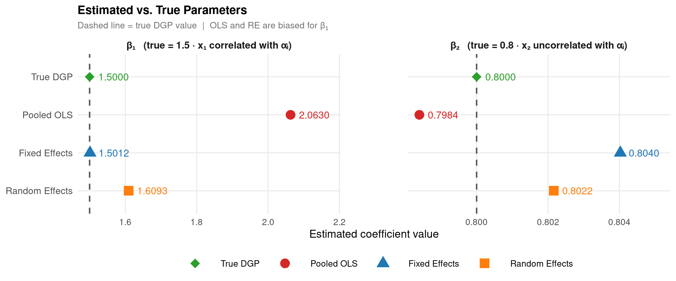
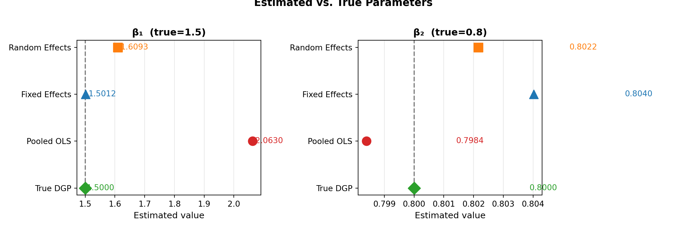
OLS attributes part of \(\text{Cov}(x_1, \alpha_i)\) to the coefficient. High-\(\alpha_i\) individuals tend to have high \(x_1\) (\(\rho=0.6\)), so OLS confounds individual ability with \(x_1\)’s effect.

Note

Why is \(\hat{\beta}_2\) unaffected?

\(x_2 \perp \alpha_i\) by construction. All three estimators are consistent for \(\beta_2 = 0.8\).

Results — Tabular Format

modelsummary(
  list("Pooled OLS" = ols_r, "Fixed Effects" = fe_r, "Random Effects" = re_r),
  stars    = TRUE,
  gof_omit = "IC|Log|F|RMSE",
  notes    = "SEs in parentheses. *** p<0.01, ** p<0.05, * p<0.1",
  title    = "Panel Regression Results"
)

Panel Regression Results
	Pooled OLS	Fixed Effects	Random Effects
+ p < 0.1, * p < 0.05, p < 0.01, * p < 0.001
SEs in parentheses. * p<0.01, p<0.05, * p<0.1
(Intercept)	-0.036		-0.066+
	(0.027)		(0.038)
x1	2.063***	1.501***	1.609***
	(0.021)	(0.014)	(0.016)
x2	0.798***	0.804***	0.802***
	(0.017)	(0.009)	(0.011)
Num.Obs.	2000	2000	2000
R2	0.854	0.917	0.889
R2 Adj.	0.854	0.907	0.889

print(compare({"Pooled OLS": ols_py, "FE": fe_py, "RE": re_py}))

                            Model Comparison                           
=======================================================================
                            Pooled OLS             FE                RE
-----------------------------------------------------------------------
Dep. Variable                        y              y                 y
Estimator                    PooledOLS       PanelOLS     RandomEffects
No. Observations                  2000           2000              2000
Cov. Est.                   Unadjusted     Unadjusted        Unadjusted
R-squared                       0.8539         0.9166            0.8893
R-Squared (Within)              0.8398         0.9166            0.9138
R-Squared (Between)             0.8638         0.7467            0.7549
R-Squared (Overall)             0.8539         0.8127            0.8203
F-statistic                     5837.4         9885.3            8020.6
P-value (F-stat)                0.0000         0.0000            0.0000
=====================     ============   ============   ===============
const                          -0.0358                          -0.0658
                             (-1.3229)                        (-1.7477)
x1                              2.0630         1.5012            1.6093
                              (97.474)       (108.77)          (101.93)
x2                              0.7984         0.8040            0.8022
                              (45.748)       (86.399)          (72.911)
======================= ============== ============== =================
Effects                                        Entity                  
-----------------------------------------------------------------------

T-stats reported in parentheses

quietly import delimited "../data/panel-OLS-FE-RE.csv", clear
quietly xtset id time
quietly regress y x1 x2
quietly estimates store OLS
quietly xtreg y x1 x2, fe
quietly estimates store FE
quietly xtreg y x1 x2, re
quietly estimates store RE
esttab OLS FE RE,                                            ///
    b(4) se(4) star(* 0.10 ** 0.05 *** 0.01)                 ///
    stats(N r2_w r2_b r2_o,                                  ///
          labels("N" "R² within" "R² between" "R² overall")  ///
          fmt(0 3 3 3))                                      ///
    title("Panel Regression Results")                        ///
    mtitles("Pooled OLS" "Fixed Effects" "Random Effects")   ///
    note("SEs in parentheses.  * p<0.10  ** p<0.05  *** p<0.01")

Panel Regression Results
------------------------------------------------------------
                      (1)             (2)             (3)   
               Pooled OLS    Fixed Effe~s    Random Eff~s   
------------------------------------------------------------
x1                 2.0630***       1.5012***       1.6093***
                 (0.0212)        (0.0138)        (0.0158)   

x2                 0.7984***       0.8040***       0.8022***
                 (0.0175)        (0.0093)        (0.0110)   

_cons             -0.0358         -0.0739***      -0.0658*  
                 (0.0271)        (0.0141)        (0.0377)   
------------------------------------------------------------
N                    2000            2000            2000   
R² within                           0.917           0.916   
R² between                          0.936           0.940   
R² overall                          0.838           0.845   
------------------------------------------------------------
SEs in parentheses.  * p<0.10  ** p<0.05  *** p<0.01
* p<0.10, ** p<0.05, *** p<0.01

LaTeX Table Export

modelsummary(
  list("Pooled OLS" = ols_r, "Fixed Effects" = fe_r, "Random Effects" = re_r),
  stars = TRUE, gof_omit = "IC|Log|F|RMSE",
  output = "latex"
)

strs = lambda p: "***" if p<0.01 else ("**" if p<0.05 else ("*" if p<0.1 else ""))
rows = []
for nm, res in [("Pooled OLS", ols_py), ("FE", fe_py), ("RE", re_py)]:
    for v in ["x1", "x2"]:
        if v in res.params.index:
            rows.append({"Variable": v, "Model": nm,
                         "Coef": f"{res.params[v]:.4f}{strs(res.pvalues[v])}"})
pivot = pd.DataFrame(rows).pivot(index="Variable", columns="Model", values="Coef")
print(pivot.to_latex(caption="Panel Regression Results", label="tab:panel"))

\begin{table}
\caption{Panel Regression Results}
\label{tab:panel}
\begin{tabular}{llll}
\toprule
Model & FE & Pooled OLS & RE \\
Variable &  &  &  \\
\midrule
x1 & 1.5012*** & 2.0630*** & 1.6093*** \\
x2 & 0.8040*** & 0.7984*** & 0.8022*** \\
\bottomrule
\end{tabular}
\end{table}

quietly import delimited "../data/panel-OLS-FE-RE.csv", clear
quietly xtset id time
quietly regress y x1 x2
quietly estimates store OLS
quietly xtreg y x1 x2, fe
quietly estimates store FE
quietly xtreg y x1 x2, re
quietly estimates store RE
esttab OLS FE RE using "panel-results.tex",                 ///
    b(4) se(4) star(* 0.10 ** 0.05 *** 0.01)                ///
    booktabs replace                                        ///
    title("Panel Regression Results\label{tab:panel}")      ///
    mtitles("Pooled OLS" "Fixed Effects" "Random Effects")  ///
    stats(N r2_w r2_b r2_o, fmt(0 3 3 3)                    ///
          labels("$N$" "$R^2$ within" "$R^2$ between" "$R^2$ overall"))

(output written to panel-results.tex)

F-test for Fixed Effects — Theory

Null hypothesis: all individual effects are equal (pooled OLS is sufficient)

\[H_0: \alpha_1 = \alpha_2 = \cdots = \alpha_N\]

Test statistic:

\[F = \frac{(RSS_{OLS} - RSS_{FE})\,/\,(N-1)}{RSS_{FE}\,/\,(NT - N - k)} \sim F(N-1,\; NT-N-k)\]

Why needed: if the \(\alpha_i\) do not differ, pooled OLS is unbiased and efficient — FE would needlessly sacrifice \(N-1\) degrees of freedom.

Reject when: \(F > F_{1-\alpha}(N-1, NT-N-k)\) — individual effects are jointly significant → prefer FE over pooled OLS.

F-test for Fixed Effects — Code

pFtest(fe_r, ols_r)


    F test for individual effects

data:  y ~ x1 + x2
F = 29.417, df1 = 199, df2 = 1798, p-value < 2.2e-16
alternative hypothesis: significant effects

y_arr     = y_p.to_numpy().ravel()
yhat_arr  = ols_py.fitted_values.to_numpy().ravel()
resid_fe  = fe_py.resids.to_numpy().ravel()
resid_ols = y_arr - yhat_arr
N_i, T_i, k_i = 200, 10, 2;  NT_i = N_i * T_i
RSS_fe  = float(np.dot(resid_fe, resid_fe))
RSS_ols = float(np.dot(resid_ols, resid_ols))
F_stat  = float(((RSS_ols - RSS_fe) / (N_i - 1)) / (RSS_fe / (NT_i - N_i - k_i)))
p_F     = float(1 - f_dist.cdf(F_stat, N_i - 1, NT_i - N_i - k_i))
print(f"F({N_i-1}, {NT_i-N_i-k_i}) = {F_stat:.4f},  p-value = {p_F:.3e}")

F(199, 1798) = 29.4166,  p-value = 1.110e-16

print("Decision:", "Reject H₀ → FE preferred" if p_F < 0.05 else "Do not reject H₀")

Decision: Reject H₀ → FE preferred

quietly import delimited "../data/panel-OLS-FE-RE.csv", clear
quietly xtset id time
* The F-test appears automatically at the bottom of xtreg, fe output
xtreg y x1 x2, fe
* "F test that all u_i=0: F(N-1, NT-N-k)  Prob > F = ..."

Fixed-effects (within) regression               Number of obs     =      2,000
Group variable: id                              Number of groups  =        200

R-squared:                                      Obs per group:
     Within  = 0.9166                                         min =         10
     Between = 0.9363                                         avg =       10.0
     Overall = 0.8382                                         max =         10

                                                F(2, 1798)        =    9885.30
corr(u_i, Xb) = 0.4682                          Prob > F          =     0.0000

------------------------------------------------------------------------------
           y | Coefficient  Std. err.      t    P>|t|     [95% conf. interval]
-------------+----------------------------------------------------------------
          x1 |    1.50115   .0138017   108.77   0.000     1.474081    1.528219
          x2 |   .8040246   .0093059    86.40   0.000      .785773    .8222762
       _cons |   -.073891   .0140755    -5.25   0.000    -.1014971   -.0462848
-------------+----------------------------------------------------------------
     sigma_u |  1.0066421
     sigma_e |  .48552911
         rho |  .81126828   (fraction of variance due to u_i)
------------------------------------------------------------------------------
F test that all u_i=0: F(199, 1798) = 29.42                  Prob > F = 0.0000

Breusch-Pagan LM Test — Theory

Null hypothesis: no random individual effects (pooled OLS is sufficient)

\[H_0: \sigma_\alpha^2 = 0\]

Test statistic (Breusch & Pagan, 1980):

\[LM = \frac{NT}{2(T-1)}\left[\frac{\sum_i \left(\sum_t \hat{u}_{it}\right)^2}{\sum_{i,t} \hat{u}_{it}^2} - 1\right]^2 \sim \chi^2(1)\]

Why needed: detects whether the composite error contains an individual component at all — computed from pooled OLS residuals only.

Reject when: \(LM > \chi^2_{1-\alpha}(1)\) — random effects exist → prefer RE (or FE) over pooled OLS.

Breusch-Pagan LM Test — Code

ols_plm <- plm(y ~ x1 + x2, data = pdf, model = "pooling")
plmtest(ols_plm, effect = "individual", type = "bp")


    Lagrange Multiplier Test - (Breusch-Pagan)

data:  y ~ x1 + x2
chisq = 2234.5, df = 1, p-value < 2.2e-16
alternative hypothesis: significant effects

resid_s = pd.Series(resid_ols, index=y_p.index)
g_sum   = resid_s.groupby(level="id").sum()
LM      = float((NT_i / (2*(T_i - 1))) *
                ((g_sum**2).sum() / (resid_ols**2).sum() - 1)**2)
p_LM    = float(1 - chi2_dist.cdf(LM, df=1))
print(f"LM = {LM:.4f},  p-value = {p_LM:.3e}")

LM = 2234.4923,  p-value = 0.000e+00

print("Decision:", "Reject H₀ → RE present" if p_LM < 0.05 else "Do not reject H₀")

Decision: Reject H₀ → RE present

quietly import delimited "../data/panel-OLS-FE-RE.csv", clear
quietly xtset id time
quietly xtreg y x1 x2, re
xttest0

Breusch and Pagan Lagrangian multiplier test for random effects

        y[id,t] = Xb + u[id] + e[id,t]

        Estimated results:
                         |       Var     SD = sqrt(Var)
                ---------+-----------------------------
                       y |   6.177771       2.485512
                       e |   .2357385       .4855291
                       u |   .1611694       .4014591

        Test: Var(u) = 0
                             chibar2(01) =  2234.49
                          Prob > chibar2 =   0.0000

Hausman Specification Test — Theory

Null hypothesis: the individual effects are uncorrelated with the regressors (RE is consistent and efficient)

\[H_0: \text{Cov}(\alpha_i, \mathbf{x}_{it}) = 0\]

Test statistic:

\[H = (\hat{\boldsymbol{\beta}}_{FE} - \hat{\boldsymbol{\beta}}_{RE})^\top \left[\widehat{\text{Var}}(\hat{\boldsymbol{\beta}}_{FE}) - \widehat{\text{Var}}(\hat{\boldsymbol{\beta}}_{RE})\right]^{-1} (\hat{\boldsymbol{\beta}}_{FE} - \hat{\boldsymbol{\beta}}_{RE}) \sim \chi^2(k)\]

Why needed: under \(H_0\) both FE and RE are consistent (use RE — more efficient); under \(H_1\) only FE is consistent. The test compares the two estimates directly.

Reject when: \(H > \chi^2_{1-\alpha}(k)\) — the FE and RE estimates diverge systematically → use FE.

Hausman Specification Test — Code

phtest(fe_r, re_r)


    Hausman Test

data:  y ~ x1 + x2
chisq = 198.93, df = 2, p-value < 2.2e-16
alternative hypothesis: one model is inconsistent

b_fe   = fe_py.params.to_numpy().ravel()
b_re   = re_py.params[["x1", "x2"]].to_numpy().ravel()
V_fe   = fe_py.cov.to_numpy()
V_re   = re_py.cov.loc[["x1", "x2"], ["x1", "x2"]].to_numpy()
diff   = b_fe - b_re
# abs() + pinv guard against a non-positive-definite variance difference
H_stat = float(abs(diff @ np.linalg.pinv(V_fe - V_re) @ diff))
p_H    = float(1 - chi2_dist.cdf(H_stat, df=len(diff)))
print(f"H = {H_stat:.4f},  df = {len(diff)},  p-value = {p_H:.3e}")

H = 198.9319,  df = 2,  p-value = 0.000e+00

print("Decision:", "Reject H₀ → use FE" if p_H < 0.05 else "Cannot reject → RE preferred")

Decision: Reject H₀ → use FE

quietly import delimited "../data/panel-OLS-FE-RE.csv", clear
quietly xtset id time
quietly xtreg y x1 x2, fe
estimates store FE_h
quietly xtreg y x1 x2, re
estimates store RE_h
hausman FE_h RE_h, sigmamore

                 ---- Coefficients ----
             |      (b)          (B)            (b-B)     sqrt(diag(V_b-V_B))
             |      FE_h         RE_h        Difference       Std. err.
-------------+----------------------------------------------------------------
          x1 |     1.50115     1.609284       -.1081338        .0044752
          x2 |    .8040246     .8021588        .0018658        .0011782
------------------------------------------------------------------------------
                          b = Consistent under H0 and Ha; obtained from xtreg.
           B = Inconsistent under Ha, efficient under H0; obtained from xtreg.

Test of H0: Difference in coefficients not systematic

    chi2(2) = (b-B)'[(V_b-V_B)^(-1)](b-B)
            = 585.84
Prob > chi2 = 0.0000

Test Summary

Test	H0	Statistic	p-value	Decision
F-test for FE	All \(\alpha_i\) equal (OLS ok)	29.417	<2e-16	Reject → FE
Breusch-Pagan LM	\(\sigma^2_\alpha = 0\) (OLS ok)	2234.492	<2e-16	Reject → RE/FE
Hausman	\(\text{Cov}(\alpha_i, X) = 0\) (RE consistent)	198.932	<2e-16	Reject → FE

Important

All three tests point to the same conclusion: use Fixed Effects. Individual effects are significant and correlated with \(X_{it}\); the RE assumption is violated. \(\hat{\beta}_1^{FE} \approx 1.501 \approx \beta_1^{true} = 1.5\) ✓

Variation: Clustered Standard Errors

Classical FE SEs assume \(\varepsilon_{it}\) is iid. In practice, errors are often serially correlated within individuals. Cluster-robust SEs correct for this.

\[\hat{V}_{CR}(\hat{\boldsymbol{\beta}}_{FE}) = (\tilde{X}^\top \tilde{X})^{-1} \left(\sum_{i=1}^N \tilde{\mathbf{x}}_i^\top \hat{\boldsymbol{\varepsilon}}_i \hat{\boldsymbol{\varepsilon}}_i^\top \tilde{\mathbf{x}}_i \right)(\tilde{X}^\top \tilde{X})^{-1}\]

coeftest(fe_r, vcov = vcovHC(fe_r, type = "HC1", cluster = "group"))


t test of coefficients:

    Estimate Std. Error t value  Pr(>|t|)    
x1 1.5011504  0.0134327 111.754 < 2.2e-16 ***
x2 0.8040246  0.0097967  82.071 < 2.2e-16 ***
---
Signif. codes:  0 '***' 0.001 '**' 0.01 '*' 0.05 '.' 0.1 ' ' 1

fe_cl = PanelOLS(y_p, df_py[["x1", "x2"]],
                 entity_effects=True).fit(cov_type="clustered",
                                          cluster_entity=True)
print(fe_cl.summary.tables[1])

                             Parameter Estimates                              
==============================================================================
            Parameter  Std. Err.     T-stat    P-value    Lower CI    Upper CI
------------------------------------------------------------------------------
x1             1.5012     0.0134     111.75     0.0000      1.4748      1.5275
x2             0.8040     0.0098     82.071     0.0000      0.7848      0.8232
==============================================================================

quietly import delimited "../data/panel-OLS-FE-RE.csv", clear
quietly xtset id time
xtreg y x1 x2, fe vce(cluster id)

Fixed-effects (within) regression               Number of obs     =      2,000
Group variable: id                              Number of groups  =        200

R-squared:                                      Obs per group:
     Within  = 0.9166                                         min =         10
     Between = 0.9363                                         avg =       10.0
     Overall = 0.8382                                         max =         10

                                                F(2, 199)         =    9672.25
corr(u_i, Xb) = 0.4682                          Prob > F          =     0.0000

                                   (Std. err. adjusted for 200 clusters in id)
------------------------------------------------------------------------------
             |               Robust
           y | Coefficient  std. err.      t    P>|t|     [95% conf. interval]
-------------+----------------------------------------------------------------
          x1 |    1.50115   .0134664   111.47   0.000     1.474595    1.527706
          x2 |   .8040246   .0098213    81.87   0.000     .7846574    .8233918
       _cons |   -.073891   .0094372    -7.83   0.000    -.0925008   -.0552812
-------------+----------------------------------------------------------------
     sigma_u |  1.0066421
     sigma_e |  .48552911
         rho |  .81126828   (fraction of variance due to u_i)
------------------------------------------------------------------------------

Variation: First Differences

Alternative to FE: eliminate \(\alpha_i\) by differencing consecutive periods:

\[\Delta y_{it} = \beta_1 \Delta x_{1,it} + \beta_2 \Delta x_{2,it} + \Delta\varepsilon_{it}, \quad t = 2,\ldots,T\]

Condition	Prefer
\(\varepsilon_{it}\) is iid	FE (uses all \(T\) observations per person)
\(\varepsilon_{it}\) follows a random walk	FD (more robust to unit roots)
\(T = 2\)	FD ≡ FE

fd_r <- plm(y ~ x1 + x2, data = pdf, model = "fd")
tidy(fd_r) %>%
  kbl(digits = 4) %>%
  kable_styling(font_size = 15)

term	estimate	std.error	statistic	p.value
(Intercept)	0.0029	0.0162	0.1767	0.8598
x1	1.5052	0.0138	109.3835	0.0000
x2	0.8110	0.0093	87.0787	0.0000

fd_py = FirstDifferenceOLS(y_p, df_py[["x1", "x2"]]).fit()
print(fd_py.summary.tables[1])

                             Parameter Estimates                              
==============================================================================
            Parameter  Std. Err.     T-stat    P-value    Lower CI    Upper CI
------------------------------------------------------------------------------
x1             1.5051     0.0138     109.42     0.0000      1.4782      1.5321
x2             0.8110     0.0093     87.102     0.0000      0.7928      0.8293
==============================================================================

quietly import delimited "../data/panel-OLS-FE-RE.csv", clear
quietly xtset id time
gen dy  = d.y
gen dx1 = d.x1
gen dx2 = d.x2
regress dy dx1 dx2, noconstant vce(cluster id)

(200 missing values generated)

(200 missing values generated)

(200 missing values generated)


Linear regression                               Number of obs     =      1,800
                                                F(2, 199)         =    6987.69
                                                Prob > F          =     0.0000
                                                R-squared         =     0.9188
                                                Root MSE          =      .6859

                                   (Std. err. adjusted for 200 clusters in id)
------------------------------------------------------------------------------
             |               Robust
          dy | Coefficient  std. err.      t    P>|t|     [95% conf. interval]
-------------+----------------------------------------------------------------
         dx1 |   1.505147   .0167414    89.91   0.000     1.472134     1.53816
         dx2 |   .8110255   .0105181    77.11   0.000     .7902843    .8317667
------------------------------------------------------------------------------

Variation: Mundlak Correction

Idea (Mundlak, 1978): Include individual means \(\bar{\mathbf{x}}_i\) in a RE model to absorb the correlation between \(\alpha_i\) and \(X_{it}\).

\[y_{it} = \mu + \beta_1 x_{1,it} + \beta_2 x_{2,it} + \underbrace{\gamma_1 \bar{x}_{1,i} + \gamma_2 \bar{x}_{2,i}}_{\text{Mundlak terms}} + v_i + \varepsilon_{it}\]

If \(\gamma_j \neq 0\) → FE preferred. The slopes \(\hat{\beta}_j\) are numerically identical to FE.

df_m  <- df %>%
  group_by(id) %>%
  mutate(x1_bar = mean(x1), x2_bar = mean(x2)) %>%
  ungroup()
pdf_m <- pdata.frame(df_m, index = c("id", "time"))
mundlak_r <- plm(y ~ x1 + x2 + x1_bar + x2_bar, data = pdf_m, model = "random")
tidy(mundlak_r) %>%
  kbl(digits = 4) %>%
  kable_styling(font_size = 15)

term	estimate	std.error	statistic	p.value
(Intercept)	-0.1067	0.0889	-1.2003	0.2300
x1	1.5012	0.0138	108.7657	0.0000
x2	0.8040	0.0093	86.3991	0.0000
x1_bar	1.4592	0.0507	28.7786	0.0000
x2_bar	0.1231	0.0880	1.3999	0.1615

dm2 = df_py.reset_index()
dm2["x1_bar"] = dm2.groupby("id")["x1"].transform("mean")
dm2["x2_bar"] = dm2.groupby("id")["x2"].transform("mean")
dm2 = dm2.set_index(["id", "time"])
Xm  = sm.add_constant(dm2[["x1", "x2", "x1_bar", "x2_bar"]])
print(RandomEffects(dm2["y"], Xm).fit().summary.tables[1])

                             Parameter Estimates                              
==============================================================================
            Parameter  Std. Err.     T-stat    P-value    Lower CI    Upper CI
------------------------------------------------------------------------------
const         -0.1067     0.0893    -1.1954     0.2321     -0.2819      0.0684
x1             1.5012     0.0138     108.81     0.0000      1.4741      1.5282
x2             0.8040     0.0093     86.438     0.0000      0.7858      0.8223
x1_bar         1.4592     0.0509     28.670     0.0000      1.3594      1.5590
x2_bar         0.1231     0.0883     1.3943     0.1634     -0.0501      0.2964
==============================================================================

quietly {
    import delimited "../data/panel-OLS-FE-RE.csv", clear
    xtset id time
    bysort id: egen x1_bar = mean(x1)
    bysort id: egen x2_bar = mean(x2)
}
xtreg y x1 x2 x1_bar x2_bar, re
* Significant x1_bar/x2_bar confirms Cov(alpha_i, X) != 0  →  use FE

Random-effects GLS regression                   Number of obs     =      2,000
Group variable: id                              Number of groups  =        200

R-squared:                                      Obs per group:
     Within  = 0.9166                                         min =         10
     Between = 0.9499                                         avg =       10.0
     Overall = 0.9362                                         max =         10

                                                Wald chi2(4)      =   23505.99
corr(u_i, X) = 0 (assumed)                      Prob > chi2       =     0.0000

------------------------------------------------------------------------------
           y | Coefficient  Std. err.      z    P>|z|     [95% conf. interval]
-------------+----------------------------------------------------------------
          x1 |    1.50115   .0138017   108.77   0.000       1.4741    1.528201
          x2 |   .8040246   .0093059    86.40   0.000     .7857853    .8222639
      x1_bar |   1.459163   .0507031    28.78   0.000     1.359787    1.558539
      x2_bar |   .1231477   .0879676     1.40   0.162    -.0492656     .295561
       _cons |  -.1067447   .0889302    -1.20   0.230    -.2810447    .0675553
-------------+----------------------------------------------------------------
     sigma_u |   .4014591
     sigma_e |  .48552911
         rho |  .40606246   (fraction of variance due to u_i)
------------------------------------------------------------------------------

Empirical Applications

πάντως δὲ κἀκεῖ ταῦτʼ ἔδρας ἑκάστοτε.

and you did exactly this there too, every single time

Ἀριστοφάνης, Σφῆκες 770

Data Access

library(wooldridge)
data("wagepan"); data("crime4"); data("jtrain")
# Export for the Python session (R creates all shared data)
write_csv(wagepan, "../data/wagepan.csv")
write_csv(crime4,  "../data/crime4.csv")
write_csv(jtrain,  "../data/jtrain.csv")

# Python reads the CSVs exported by R
wagepan_py = pd.read_csv("../data/wagepan.csv").set_index(["nr", "year"])
crime4_py  = pd.read_csv("../data/crime4.csv").set_index(["county", "year"])
jtrain_py  = (pd.read_csv("../data/jtrain.csv")
                .dropna(subset=["lscrap"])
                .set_index(["fcode", "year"]))
print(f"wagepan: {wagepan_py.shape} | crime4: {crime4_py.shape} | jtrain: {jtrain_py.shape}")

wagepan: (4360, 42) | crime4: (630, 57) | jtrain: (162, 28)

* Stata reads the original .dta files from the Boston College archive
quietly use "http://fmwww.bc.edu/ec-p/data/wooldridge/wagepan.dta", clear
quietly use "http://fmwww.bc.edu/ec-p/data/wooldridge/crime4.dta", clear
quietly use "http://fmwww.bc.edu/ec-p/data/wooldridge/jtrain.dta", clear
describe, short

Contains data from http://fmwww.bc.edu/ec-p/data/wooldridge/jtrain.dta
 Observations:           471                  
    Variables:            30                  26 Jan 2000 12:16
Sorted by:

The Three Examples — Question, Data & Model

wagepan — union premium
crime4 — county crime
jtrain — training grants

Research question: What is the wage premium from joining a union, controlling for individual ability?

The endogeneity problem. Union membership is not randomly assigned. Workers with higher unobservable productivity — motivation, reliability, cognitive skill — are more likely to join (or be accepted by) unions and earn higher wages regardless of union status. A naive cross-sectional regression conflates the union wage effect with the selection effect:

\[\underbrace{\text{Cov}(union_{it},\, \alpha_i)}_{\text{selection: } > 0} \neq 0 \implies \hat{\beta}_{OLS} \text{ is biased upward}\]

Panel solution. With repeated observations of the same worker, we can difference out \(\alpha_i\) (time-invariant ability). Fixed Effects identifies the union premium only from workers who change union status over the panel — a within-person comparison free of selection bias.

Tip

Wooldridge reference: Table 14.2, p. 484 (7th ed.). The OLS union premium (≈ 18%) drops by more than half under FE (≈ 8%), a concrete illustration of ability bias.

Source: National Longitudinal Survey of Young Men (NLSY), 1980–1987. Structure: Balanced panel — \(N = 545\) men, \(T = 8\) years, \(NT = 4{,}360\) observations.

Variable	Description	Type
`nr`	Individual identifier	ID
`year`	Survey year (1980–1987)	Time
`lwage`	Log hourly wage (outcome)	Continuous
`union`	= 1 if union member	Time-varying
`married`	= 1 if married	Time-varying
`exper`, `expersq`	Experience (years) & its square	Time-varying
`educ`	Years of schooling	Time-invariant
`black`, `hisp`	Race/ethnicity indicators	Time-invariant
`d81`–`d87`	Year dummies (base = 1980)	Time fixed effects

Warning

educ, black, and hisp are time-invariant — Fixed Effects cannot identify their coefficients (they are absorbed into \(\hat{\alpha}_i\)). Only OLS and RE can estimate them.

\[\log(wage_{it}) = \alpha_i + \beta_1\, union_{it} + \beta_2\, married_{it} + \beta_3\, exper_{it} + \beta_4\, exper_{it}^2 + \gamma_1\, educ_i + \gamma_2\, black_i + \gamma_3\, hisp_i + \sum_{s=1981}^{1987}\delta_s\, d_{st} + \varepsilon_{it}\]

Endogeneity structure:

\[\underbrace{\text{Cov}(union_{it},\, \alpha_i) > 0}_{\text{productive workers join unions}} \implies \hat{\beta}_1^{OLS} > \hat{\beta}_1^{FE}\]

Estimator comparison:

Estimator	Identifies \(\beta_1\)?	Identifies \(\gamma_1\) (educ)?	Variation used
Pooled OLS	Biased ✗	✓	Between + Within
Fixed Effects	Consistent ✓	✗ (dropped)	Within only
Random Effects	Consistent only if \(\alpha_i \perp X\)	✓	Between + Within

Research question: Does increasing police presence reduce crime, and by how much?

The endogeneity problem. Police are deployed in response to crime: counties with chronically high crime rates hire more officers. This reverse causality means Pooled OLS will show a positive correlation between police and crime — the opposite of the deterrence effect. Time-invariant county characteristics (geography, population density, culture, historical crime patterns) compound the problem.

\[\underbrace{\text{Cov}(polpc_{it},\, \alpha_i)}_{\text{high-crime counties hire more police}} \neq 0 \implies \hat{\beta}^{OLS}_{polpc} \text{ is biased upward (or even sign-reversed)}\]

Panel solution. County fixed effects absorb all time-invariant characteristics. The within-county variation in policing over time, after controlling for economic conditions, identifies the deterrence effect free of cross-sectional confounding.

Tip

Wooldridge reference: Table 13.3, p. 438 (7th ed.). The OLS coefficient on lpolpc is positive; the FE coefficient changes markedly — an illustration of omitted variable bias from stable county characteristics.

Source: Cornwell & Trumbull (1994), North Carolina county crime data. Structure: Balanced panel — \(N = 90\) counties, \(T = 7\) years (1981–1987), \(NT = 630\) observations.

Variable	Description	Type
`county`	County identifier	ID
`year`	Year (1981–1987)	Time
`lcrmrte`	Log crime rate per person (outcome)	Continuous
`lpolpc`	Log police per capita	Time-varying
`ldensity`	Log population density	Mostly time-invariant
`lwcon`	Log weekly wage in construction	Time-varying
`lwser`	Log weekly wage in services	Time-varying
`lwtrd`	Log weekly wage in trade	Time-varying
`d82`–`d87`	Year dummies (base = 1981)	Time fixed effects

Economic intuition: wage variables capture the opportunity cost of crime (higher wages → higher cost of incarceration → less crime). County fixed effects capture all time-invariant characteristics: geography, culture, historical crime environment.

\[\log(crmrte_{it}) = \alpha_i + \lambda_t + \beta_1\,\log(polpc_{it}) + \beta_2\,\log(density_{it}) + \beta_3\,\log(wcon_{it}) + \beta_4\,\log(wser_{it}) + \beta_5\,\log(wtrd_{it}) + \sum_{s=1982}^{1987}\delta_s\,d_{st} + \varepsilon_{it}\]

Sign predictions:

\[\beta_1 < 0 \text{ (deterrence)}, \quad \beta_3, \beta_4, \beta_5 < 0 \text{ (higher wages → lower crime)}\]

Endogeneity:

\[\text{Cov}(\log polpc_{it},\, \alpha_i) > 0 \text{ because counties with high } \alpha_i \text{ (crime culture) hire more police}\]

\[\implies \hat{\beta}_1^{OLS} \neq \hat{\beta}_1^{FE} \quad \text{(OLS confounds deterrence with reverse causality)}\]

Identification in FE comes from within-county changes in police staffing over time — a policy-relevant source of variation free of cross-sectional selection.

Research question: Does government-funded job training reduce production defects (scrap)?

The endogeneity problem. Grant receipt is not random. Two opposing selection mechanisms may operate simultaneously:

Negative selection: poorly-performing firms are targeted for grants (or more likely to apply for remedial training) → \(\text{Cov}(grant_{it}, \alpha_i) < 0\) → OLS under-estimates the training effect
Positive selection: better-managed firms have the administrative capacity to apply for grants → \(\text{Cov}(grant_{it}, \alpha_i) > 0\) → OLS over-estimates the effect

Without knowing which dominates, OLS is unreliable in either direction.

Panel solution. Firm fixed effects absorb management quality (\(\alpha_i\)). The within-firm change in scrap rate after receiving a grant — compared to the same firm before — identifies the causal training effect.

Tip

Wooldridge reference: Table 13.8, p. 444 (7th ed.). \(T = 3\) (1987–1989), \(N = 54\) firms with complete lscrap data. The FE estimate of grant is negative and substantially larger in magnitude than OLS.

Source: Holzer et al. (1993), Michigan manufacturing firms. Structure: Unbalanced panel (after dropping missing lscrap) — \(T = 3\) years (1987–1989), \(N = 54\) firms with complete scrap data.

Variable	Description	Type
`fcode`	Firm identifier	ID
`year`	Survey year (1987–1989)	Time
`lscrap`	Log scrap rate (defects per 100 items, outcome)	Continuous
`grant`	= 1 if firm received training grant this year	Time-varying
`grant_1`	= 1 if firm received grant in previous year	Time-varying
`d88`, `d89`	Year dummies (base = 1987)	Time fixed effects

Warning

lscrap has many missing values — only firms that voluntarily reported scrap rates are included. This selective reporting may introduce attrition bias; results should be interpreted cautiously.

Expected sign: \(\beta_1 < 0\) — training reduces defects (lower scrap = higher productivity). \(\beta_2 \leq 0\) — any lagged effect of prior-year grant.

\[\log(scrap_{it}) = \alpha_i + \beta_1\, grant_{it} + \beta_2\, grant_{i,t-1} + \delta_1\, d88_t + \delta_2\, d89_t + \varepsilon_{it}\]

Identification under FE: Demeaning gives \(\widetilde{\log(scrap)}_{it} = \beta_1\, \widetilde{grant}_{it} + \beta_2\, \widetilde{grant}_{1,it} + \ldots\) The within-firm variation in grant receipt identifies \(\beta_1\) — controlling for all stable firm characteristics: management quality, capital stock, product complexity, industry.

Endogeneity structure:

\[\text{Cov}(grant_{it},\, \alpha_i) \neq 0 \text{ (direction ambiguous)} \implies \hat{\beta}_1^{OLS} \neq \hat{\beta}_1^{FE}\]

Key test: The Hausman test determines whether the correlation between \(\alpha_i\) and \(grant_{it}\) is large enough to make RE inconsistent.

wagepan_r <- wagepan
pdf_w     <- pdata.frame(wagepan_r, index = c("nr", "year"))
ols_w <- lm(lwage ~ union + married + exper + expersq +
              educ + black + hisp + d81 + d82 + d83 + d84 + d85 + d86 + d87,
            data = wagepan_r)
summary(ols_w)


Call:
lm(formula = lwage ~ union + married + exper + expersq + educ + 
    black + hisp + d81 + d82 + d83 + d84 + d85 + d86 + d87, data = wagepan_r)

Residuals:
    Min      1Q  Median      3Q     Max 
-5.2657 -0.2484  0.0319  0.2947  2.5291 

Coefficients:
             Estimate Std. Error t value Pr(>|t|)    
(Intercept)  0.092056   0.078270   1.176 0.239608    
union        0.182461   0.017157  10.635  < 2e-16 ***
married      0.108253   0.015689   6.900 5.96e-12 ***
exper        0.067235   0.013695   4.909 9.47e-07 ***
expersq     -0.002412   0.000820  -2.941 0.003286 ** 
educ         0.091350   0.005237  17.442  < 2e-16 ***
black       -0.139234   0.023580  -5.905 3.80e-09 ***
hisp         0.016019   0.020797   0.770 0.441179    
d81          0.058320   0.030354   1.921 0.054753 .  
d82          0.062774   0.033214   1.890 0.058825 .  
d83          0.062012   0.036660   1.692 0.090807 .  
d84          0.090467   0.040091   2.257 0.024085 *  
d85          0.109246   0.043353   2.520 0.011773 *  
d86          0.141960   0.046423   3.058 0.002242 ** 
d87          0.173833   0.049433   3.517 0.000442 ***
---
Signif. codes:  0 '***' 0.001 '**' 0.01 '*' 0.05 '.' 0.1 ' ' 1

Residual standard error: 0.4803 on 4345 degrees of freedom
Multiple R-squared:  0.1893,    Adjusted R-squared:  0.1867 
F-statistic: 72.46 on 14 and 4345 DF,  p-value: < 2.2e-16

y_w  = wagepan_py["lwage"]
Xo_w = sm.add_constant(wagepan_py[["union", "married", "exper", "expersq",
                                   "educ", "black", "hisp",
                                   "d81", "d82", "d83", "d84", "d85", "d86", "d87"]])
ols_py_w = PooledOLS(y_w, Xo_w).fit(cov_type="unadjusted")
print(ols_py_w.summary.tables[1])

                             Parameter Estimates                              
==============================================================================
            Parameter  Std. Err.     T-stat    P-value    Lower CI    Upper CI
------------------------------------------------------------------------------
const          0.0921     0.0783     1.1761     0.2396     -0.0614      0.2455
union          0.1825     0.0172     10.635     0.0000      0.1488      0.2161
married        0.1083     0.0157     6.8997     0.0000      0.0775      0.1390
exper          0.0672     0.0137     4.9095     0.0000      0.0404      0.0941
expersq       -0.0024     0.0008    -2.9413     0.0033     -0.0040     -0.0008
educ           0.0913     0.0052     17.442     0.0000      0.0811      0.1016
black         -0.1392     0.0236    -5.9049     0.0000     -0.1855     -0.0930
hisp           0.0160     0.0208     0.7703     0.4412     -0.0248      0.0568
d81            0.0583     0.0304     1.9214     0.0548     -0.0012      0.1178
d82            0.0628     0.0332     1.8900     0.0588     -0.0023      0.1279
d83            0.0620     0.0367     1.6915     0.0908     -0.0099      0.1339
d84            0.0905     0.0401     2.2566     0.0241      0.0119      0.1691
d85            0.1092     0.0434     2.5200     0.0118      0.0243      0.1942
d86            0.1420     0.0464     3.0580     0.0022      0.0509      0.2330
d87            0.1738     0.0494     3.5165     0.0004      0.0769      0.2707
==============================================================================

quietly use "http://fmwww.bc.edu/ec-p/data/wooldridge/wagepan.dta", clear
quietly xtset nr year
regress lwage union married exper expersq educ black hisp d81 d82 d83 d84 d85 d86 d87
estimates store OLS_w

      Source |       SS           df       MS      Number of obs   =     4,360
-------------+----------------------------------   F(14, 4345)     =     72.46
       Model |  234.048258        14  16.7177327   Prob > F        =    0.0000
    Residual |  1002.48136     4,345  .230720682   R-squared       =    0.1893
-------------+----------------------------------   Adj R-squared   =    0.1867
       Total |  1236.52962     4,359  .283672774   Root MSE        =    .48033

------------------------------------------------------------------------------
       lwage | Coefficient  Std. err.      t    P>|t|     [95% conf. interval]
-------------+----------------------------------------------------------------
       union |   .1824613   .0171568    10.63   0.000     .1488252    .2160973
     married |    .108253   .0156894     6.90   0.000     .0774937    .1390122
       exper |   .0672345   .0136948     4.91   0.000     .0403856    .0940834
     expersq |  -.0024117     .00082    -2.94   0.003    -.0040192   -.0008042
        educ |   .0913498   .0052374    17.44   0.000     .0810819    .1016177
       black |  -.1392342   .0235796    -5.90   0.000    -.1854622   -.0930063
        hisp |   .0160195   .0207971     0.77   0.441    -.0247535    .0567925
         d81 |     .05832   .0303536     1.92   0.055    -.0011886    .1178286
         d82 |   .0627744   .0332141     1.89   0.059    -.0023421    .1278909
         d83 |   .0620117   .0366601     1.69   0.091    -.0098608    .1338843
         d84 |   .0904672   .0400907     2.26   0.024     .0118689    .1690654
         d85 |   .1092463   .0433525     2.52   0.012     .0242533    .1942392
         d86 |   .1419595    .046423     3.06   0.002     .0509468    .2329723
         d87 |   .1738334    .049433     3.52   0.000     .0769194    .2707474
       _cons |   .0920558   .0782701     1.18   0.240    -.0613935    .2455051
------------------------------------------------------------------------------

crime4_r <- crime4
pdf_c    <- pdata.frame(crime4_r, index = c("county", "year"))
ols_c <- lm(lcrmrte ~ lpolpc + ldensity + lwcon + lwser + lwtrd +
              d82 + d83 + d84 + d85 + d86 + d87, data = crime4_r)
summary(ols_c)


Call:
lm(formula = lcrmrte ~ lpolpc + ldensity + lwcon + lwser + lwtrd + 
    d82 + d83 + d84 + d85 + d86 + d87, data = crime4_r)

Residuals:
     Min       1Q   Median       3Q      Max 
-2.46283 -0.23311 -0.00395  0.25372  2.07595 

Coefficients:
             Estimate Std. Error t value Pr(>|t|)    
(Intercept) -3.543527   0.690486  -5.132 3.85e-07 ***
lpolpc       0.116650   0.032373   3.603 0.000339 ***
ldensity     0.472771   0.026406  17.904  < 2e-16 ***
lwcon        0.042525   0.084828   0.501 0.616330    
lwser       -0.004471   0.050969  -0.088 0.930134    
lwtrd        0.111869   0.096808   1.156 0.248298    
d82         -0.010028   0.062865  -0.160 0.873310    
d83         -0.103683   0.063430  -1.635 0.102641    
d84         -0.173982   0.065757  -2.646 0.008356 ** 
d85         -0.181016   0.067201  -2.694 0.007259 ** 
d86         -0.129165   0.068584  -1.883 0.060127 .  
d87         -0.065069   0.072035  -0.903 0.366721    
---
Signif. codes:  0 '***' 0.001 '**' 0.01 '*' 0.05 '.' 0.1 ' ' 1

Residual standard error: 0.4207 on 618 degrees of freedom
Multiple R-squared:  0.4701,    Adjusted R-squared:  0.4606 
F-statistic: 49.84 on 11 and 618 DF,  p-value: < 2.2e-16

y_c  = crime4_py["lcrmrte"]
Xo_c = sm.add_constant(crime4_py[["lpolpc", "ldensity", "lwcon", "lwser", "lwtrd",
                                  "d82", "d83", "d84", "d85", "d86", "d87"]])
ols_py_c = PooledOLS(y_c, Xo_c).fit(cov_type="unadjusted")
print(ols_py_c.summary.tables[1])

                             Parameter Estimates                              
==============================================================================
            Parameter  Std. Err.     T-stat    P-value    Lower CI    Upper CI
------------------------------------------------------------------------------
const         -3.5435     0.6905    -5.1319     0.0000     -4.8995     -2.1875
lpolpc         0.1167     0.0324     3.6034     0.0003      0.0531      0.1802
ldensity       0.4728     0.0264     17.904     0.0000      0.4209      0.5246
lwcon          0.0425     0.0848     0.5013     0.6163     -0.1241      0.2091
lwser         -0.0045     0.0510    -0.0877     0.9301     -0.1046      0.0956
lwtrd          0.1119     0.0968     1.1556     0.2483     -0.0782      0.3020
d82           -0.0100     0.0629    -0.1595     0.8733     -0.1335      0.1134
d83           -0.1037     0.0634    -1.6346     0.1026     -0.2282      0.0209
d84           -0.1740     0.0658    -2.6458     0.0084     -0.3031     -0.0448
d85           -0.1810     0.0672    -2.6936     0.0073     -0.3130     -0.0490
d86           -0.1292     0.0686    -1.8833     0.0601     -0.2639      0.0055
d87           -0.0651     0.0720    -0.9033     0.3667     -0.2065      0.0764
==============================================================================

quietly use "http://fmwww.bc.edu/ec-p/data/wooldridge/crime4.dta", clear
quietly xtset county year
regress lcrmrte lpolpc ldensity lwcon lwser lwtrd d82 d83 d84 d85 d86 d87
estimates store OLS_c

      Source |       SS           df       MS      Number of obs   =       630
-------------+----------------------------------   F(11, 618)      =     49.84
       Model |  97.0151227        11  8.81955661   Prob > F        =    0.0000
    Residual |  109.365222       618  .176966379   R-squared       =    0.4701
-------------+----------------------------------   Adj R-squared   =    0.4606
       Total |  206.380345       629  .328108656   Root MSE        =    .42067

------------------------------------------------------------------------------
     lcrmrte | Coefficient  Std. err.      t    P>|t|     [95% conf. interval]
-------------+----------------------------------------------------------------
      lpolpc |   .1166504   .0323727     3.60   0.000     .0530766    .1802241
    ldensity |   .4727705   .0264061    17.90   0.000      .420914     .524627
       lwcon |    .042525   .0848276     0.50   0.616    -.1240603    .2091103
       lwser |  -.0044707   .0509693    -0.09   0.930    -.1045648    .0956234
       lwtrd |   .1118694   .0968076     1.16   0.248    -.0782424    .3019811
         d82 |  -.0100284   .0628648    -0.16   0.873    -.1334829    .1134262
         d83 |  -.1036831     .06343    -1.63   0.103    -.2282477    .0208814
         d84 |  -.1739818    .065757    -2.65   0.008     -.303116   -.0448476
         d85 |  -.1810165   .0672012    -2.69   0.007    -.3129868   -.0490461
         d86 |  -.1291651   .0685839    -1.88   0.060    -.2638509    .0055206
         d87 |  -.0650693   .0720354    -0.90   0.367    -.2065331    .0763945
       _cons |  -3.543526    .690486    -5.13   0.000     -4.89951   -2.187543
------------------------------------------------------------------------------

jtrain_r <- jtrain %>% filter(!is.na(lscrap))
pdf_j    <- pdata.frame(jtrain_r, index = c("fcode", "year"))
ols_j <- lm(lscrap ~ grant + grant_1 + d88 + d89, data = jtrain_r)
summary(ols_j)


Call:
lm(formula = lscrap ~ grant + grant_1 + d88 + d89, data = jtrain_r)

Residuals:
    Min      1Q  Median      3Q     Max 
-5.2026 -0.8960 -0.0846  1.0242  3.3003 

Coefficients:
            Estimate Std. Error t value Pr(>|t|)   
(Intercept)  0.59743    0.20306   2.942  0.00375 **
grant        0.20002    0.33828   0.591  0.55519   
grant_1      0.04894    0.43607   0.112  0.91079   
d88         -0.23937    0.31086  -0.770  0.44245   
d89         -0.49652    0.33793  -1.469  0.14375   
---
Signif. codes:  0 '***' 0.001 '**' 0.01 '*' 0.05 '.' 0.1 ' ' 1

Residual standard error: 1.492 on 157 degrees of freedom
Multiple R-squared:  0.01731,   Adjusted R-squared:  -0.007726 
F-statistic: 0.6914 on 4 and 157 DF,  p-value: 0.5989

y_j  = jtrain_py["lscrap"]
Xo_j = sm.add_constant(jtrain_py[["grant", "grant_1", "d88", "d89"]])
ols_py_j = PooledOLS(y_j, Xo_j).fit(cov_type="unadjusted")
print(ols_py_j.summary.tables[1])

                             Parameter Estimates                              
==============================================================================
            Parameter  Std. Err.     T-stat    P-value    Lower CI    Upper CI
------------------------------------------------------------------------------
const          0.5974     0.2031     2.9421     0.0038      0.1963      0.9985
grant          0.2000     0.3383     0.5913     0.5552     -0.4682      0.8682
grant_1        0.0489     0.4361     0.1122     0.9108     -0.8124      0.9102
d88           -0.2394     0.3109    -0.7700     0.4424     -0.8534      0.3746
d89           -0.4965     0.3379    -1.4693     0.1437     -1.1640      0.1709
==============================================================================

quietly use "http://fmwww.bc.edu/ec-p/data/wooldridge/jtrain.dta", clear
quietly keep if !missing(lscrap)
quietly xtset fcode year
regress lscrap grant grant_1 d88 d89
estimates store OLS_j

      Source |       SS           df       MS      Number of obs   =       162
-------------+----------------------------------   F(4, 157)       =      0.69
       Model |  6.15830795         4  1.53957699   Prob > F        =    0.5989
    Residual |  349.586765       157  2.22666729   R-squared       =    0.0173
-------------+----------------------------------   Adj R-squared   =   -0.0077
       Total |  355.745073       161  2.20959673   Root MSE        =    1.4922

------------------------------------------------------------------------------
      lscrap | Coefficient  Std. err.      t    P>|t|     [95% conf. interval]
-------------+----------------------------------------------------------------
       grant |   .2000196   .3382846     0.59   0.555    -.4681564    .8681957
     grant_1 |   .0489357   .4360663     0.11   0.911    -.8123777    .9102492
         d88 |  -.2393704   .3108639    -0.77   0.442    -.8533854    .3746446
         d89 |  -.4965237   .3379281    -1.47   0.144    -1.163996    .1709483
       _cons |    .597434    .203063     2.94   0.004     .1963462    .9985218
------------------------------------------------------------------------------

Fixed Effects — All Three Examples

wagepan — union premium
crime4 — county crime
jtrain — training grants

fe_w <- plm(lwage ~ union + married + exper + expersq + educ + black + hisp +
              d82 + d83 + d84 + d85 + d86 + d87,
            data = pdf_w, model = "within")
summary(fe_w)

Oneway (individual) effect Within Model

Call:
plm(formula = lwage ~ union + married + exper + expersq + educ + 
    black + hisp + d82 + d83 + d84 + d85 + d86 + d87, data = pdf_w, 
    model = "within")

Balanced Panel: n = 545, T = 8, N = 4360

Residuals:
   Min. 1st Qu.  Median 3rd Qu.    Max. 
-4.1593 -0.1253  0.0113  0.1549  1.4921 

Coefficients:
           Estimate  Std. Error t-value  Pr(>|t|)    
union    0.08000186  0.01931031  4.1430 3.503e-05 ***
married  0.04668036  0.01831044  2.5494   0.01083 *  
exper    0.15119121  0.02194893  6.8883 6.578e-12 ***
expersq -0.00518550  0.00070444 -7.3612 2.222e-13 ***
d82     -0.04941155  0.03685806 -1.3406   0.18013    
d83     -0.09912988  0.05641429 -1.7572   0.07897 .  
d84     -0.11465003  0.07713099 -1.4864   0.13725    
d85     -0.13847376  0.09845549 -1.4065   0.15967    
d86     -0.14165066  0.12026196 -1.1779   0.23893    
d87     -0.13331351  0.14253820 -0.9353   0.34970    
---
Signif. codes:  0 '***' 0.001 '**' 0.01 '*' 0.05 '.' 0.1 ' ' 1

Total Sum of Squares:    572.05
Residual Sum of Squares: 468.75
R-Squared:      0.18058
Adj. R-Squared: 0.061271
F-statistic: 83.8515 on 10 and 3805 DF, p-value: < 2.22e-16

Xf_w    = wagepan_py[["union", "married", "exper", "expersq",
                      "d82", "d83", "d84", "d85", "d86", "d87"]]
fe_py_w = PanelOLS(y_w, Xf_w, entity_effects=True).fit(cov_type="unadjusted")
print(fe_py_w.summary.tables[1])

                             Parameter Estimates                              
==============================================================================
            Parameter  Std. Err.     T-stat    P-value    Lower CI    Upper CI
------------------------------------------------------------------------------
union          0.0800     0.0193     4.1430     0.0000      0.0421      0.1179
married        0.0467     0.0183     2.5494     0.0108      0.0108      0.0826
exper          0.1512     0.0219     6.8883     0.0000      0.1082      0.1942
expersq       -0.0052     0.0007    -7.3612     0.0000     -0.0066     -0.0038
d82           -0.0494     0.0369    -1.3406     0.1801     -0.1217      0.0229
d83           -0.0991     0.0564    -1.7572     0.0790     -0.2097      0.0115
d84           -0.1147     0.0771    -1.4864     0.1372     -0.2659      0.0366
d85           -0.1385     0.0985    -1.4065     0.1597     -0.3315      0.0546
d86           -0.1417     0.1203    -1.1779     0.2389     -0.3774      0.0941
d87           -0.1333     0.1425    -0.9353     0.3497     -0.4128      0.1461
==============================================================================

quietly use "http://fmwww.bc.edu/ec-p/data/wooldridge/wagepan.dta", clear
quietly xtset nr year
xtreg lwage union married exper expersq educ black hisp d81 d82 d83 d84 d85 d86 d87, fe
* Note: educ black hisp are dropped (time-invariant within person)
estimates store FE_w

note: educ omitted because of collinearity.
note: black omitted because of collinearity.
note: hisp omitted because of collinearity.
note: d87 omitted because of collinearity.

Fixed-effects (within) regression               Number of obs     =      4,360
Group variable: nr                              Number of groups  =        545

R-squared:                                      Obs per group:
     Within  = 0.1806                                         min =          8
     Between = 0.0005                                         avg =        8.0
     Overall = 0.0635                                         max =          8

                                                F(10, 3805)       =      83.85
corr(u_i, Xb) = -0.1212                         Prob > F          =     0.0000

------------------------------------------------------------------------------
       lwage | Coefficient  Std. err.      t    P>|t|     [95% conf. interval]
-------------+----------------------------------------------------------------
       union |   .0800019   .0193103     4.14   0.000     .0421423    .1178614
     married |   .0466804   .0183104     2.55   0.011     .0107812    .0825796
       exper |   .1321464   .0098247    13.45   0.000     .1128842    .1514087
     expersq |  -.0051855   .0007044    -7.36   0.000    -.0065666   -.0038044
        educ |          0  (omitted)
       black |          0  (omitted)
        hisp |          0  (omitted)
         d81 |   .0190448   .0203626     0.94   0.350    -.0208779    .0589674
         d82 |   -.011322   .0202275    -0.56   0.576    -.0509798    .0283359
         d83 |  -.0419955   .0203205    -2.07   0.039    -.0818357   -.0021553
         d84 |  -.0384709   .0203144    -1.89   0.058    -.0782991    .0013573
         d85 |  -.0432498   .0202458    -2.14   0.033    -.0829434   -.0035563
         d86 |   -.027382   .0203863    -1.34   0.179    -.0673511    .0125872
         d87 |          0  (omitted)
       _cons |    1.02764   .0299499    34.31   0.000     .9689201    1.086359
-------------+----------------------------------------------------------------
     sigma_u |  .40092789
     sigma_e |  .35099001
         rho |  .56612235   (fraction of variance due to u_i)
------------------------------------------------------------------------------
F test that all u_i=0: F(544, 3805) = 9.64                   Prob > F = 0.0000

fe_c <- plm(lcrmrte ~ lpolpc + ldensity + lwcon + lwser + lwtrd +
              d82 + d83 + d84 + d85 + d86 + d87,
            data = pdf_c, model = "within")
summary(fe_c)

Oneway (individual) effect Within Model

Call:
plm(formula = lcrmrte ~ lpolpc + ldensity + lwcon + lwser + lwtrd + 
    d82 + d83 + d84 + d85 + d86 + d87, data = pdf_c, model = "within")

Balanced Panel: n = 90, T = 7, N = 630

Residuals:
    Min.  1st Qu.   Median  3rd Qu.     Max. 
-0.68807 -0.07379  0.00171  0.07465  0.69024 

Coefficients:
           Estimate Std. Error t-value  Pr(>|t|)    
lpolpc    0.2390231  0.0262491  9.1060 < 2.2e-16 ***
ldensity  0.8328414  0.3235439  2.5741  0.010320 *  
lwcon    -0.0420775  0.0457208 -0.9203  0.357829    
lwser     0.0153568  0.0224434  0.6842  0.494120    
lwtrd    -0.0251047  0.0475971 -0.5274  0.598108    
d82      -0.0049134  0.0243685 -0.2016  0.840285    
d83      -0.1040681  0.0254086 -4.0958 4.867e-05 ***
d84      -0.1652525  0.0286220 -5.7736 1.324e-08 ***
d85      -0.1720680  0.0314085 -5.4784 6.647e-08 ***
d86      -0.1112500  0.0338068 -3.2908  0.001066 ** 
d87      -0.0460720  0.0377466 -1.2206  0.222795    
---
Signif. codes:  0 '***' 0.001 '**' 0.01 '*' 0.05 '.' 0.1 ' ' 1

Total Sum of Squares:    17.991
Residual Sum of Squares: 13.738
R-Squared:      0.23641
Adj. R-Squared: 0.092062
F-statistic: 14.889 on 11 and 529 DF, p-value: < 2.22e-16

Xf_c    = crime4_py[["lpolpc", "ldensity", "lwcon", "lwser", "lwtrd",
                     "d82", "d83", "d84", "d85", "d86", "d87"]]
fe_py_c = PanelOLS(y_c, Xf_c, entity_effects=True).fit(cov_type="unadjusted")
print(fe_py_c.summary.tables[1])

                             Parameter Estimates                              
==============================================================================
            Parameter  Std. Err.     T-stat    P-value    Lower CI    Upper CI
------------------------------------------------------------------------------
lpolpc         0.2390     0.0262     9.1060     0.0000      0.1875      0.2906
ldensity       0.8328     0.3235     2.5741     0.0103      0.1973      1.4684
lwcon         -0.0421     0.0457    -0.9203     0.3578     -0.1319      0.0477
lwser          0.0154     0.0224     0.6842     0.4941     -0.0287      0.0594
lwtrd         -0.0251     0.0476    -0.5274     0.5981     -0.1186      0.0684
d82           -0.0049     0.0244    -0.2016     0.8403     -0.0528      0.0430
d83           -0.1041     0.0254    -4.0958     0.0000     -0.1540     -0.0542
d84           -0.1653     0.0286    -5.7736     0.0000     -0.2215     -0.1090
d85           -0.1721     0.0314    -5.4784     0.0000     -0.2338     -0.1104
d86           -0.1112     0.0338    -3.2908     0.0011     -0.1777     -0.0448
d87           -0.0461     0.0377    -1.2206     0.2228     -0.1202      0.0281
==============================================================================

quietly use "http://fmwww.bc.edu/ec-p/data/wooldridge/crime4.dta", clear
quietly xtset county year
xtreg lcrmrte lpolpc ldensity lwcon lwser lwtrd d82 d83 d84 d85 d86 d87, fe
estimates store FE_c

Fixed-effects (within) regression               Number of obs     =        630
Group variable: county                          Number of groups  =         90

R-squared:                                      Obs per group:
     Within  = 0.2364                                         min =          7
     Between = 0.4914                                         avg =        7.0
     Overall = 0.4657                                         max =          7

                                                F(11, 529)        =      14.89
corr(u_i, Xb) = -0.5693                         Prob > F          =     0.0000

------------------------------------------------------------------------------
     lcrmrte | Coefficient  Std. err.      t    P>|t|     [95% conf. interval]
-------------+----------------------------------------------------------------
      lpolpc |   .2390231   .0262491     9.11   0.000     .1874579    .2905882
    ldensity |   .8328452   .3235439     2.57   0.010     .1972567    1.468434
       lwcon |  -.0420775   .0457208    -0.92   0.358    -.1318941    .0477392
       lwser |   .0153567   .0224434     0.68   0.494    -.0287325    .0594459
       lwtrd |  -.0251048   .0475971    -0.53   0.598    -.1186072    .0683977
         d82 |  -.0049135   .0243685    -0.20   0.840    -.0527844    .0429575
         d83 |  -.1040681   .0254086    -4.10   0.000    -.1539824   -.0541539
         d84 |  -.1652527    .028622    -5.77   0.000    -.2214793    -.109026
         d85 |  -.1720682   .0314085    -5.48   0.000    -.2337688   -.1103675
         d86 |  -.1112502   .0338068    -3.29   0.001    -.1776622   -.0448382
         d87 |  -.0460723   .0377466    -1.22   0.223    -.1202239    .0280793
       _cons |  -1.679477   .3955793    -4.25   0.000    -2.456576   -.9023778
-------------+----------------------------------------------------------------
     sigma_u |  .47881132
     sigma_e |  .16114885
         rho |  .89825244   (fraction of variance due to u_i)
------------------------------------------------------------------------------
F test that all u_i=0: F(89, 529) = 41.38                    Prob > F = 0.0000

fe_j <- plm(lscrap ~ grant + grant_1 + d88 + d89,
            data = pdf_j, model = "within")
summary(fe_j)

Oneway (individual) effect Within Model

Call:
plm(formula = lscrap ~ grant + grant_1 + d88 + d89, data = pdf_j, 
    model = "within")

Balanced Panel: n = 54, T = 3, N = 162

Residuals:
   Min. 1st Qu.  Median 3rd Qu.    Max. 
-2.2869 -0.1124 -0.0178  0.1443  1.4267 

Coefficients:
         Estimate Std. Error t-value Pr(>|t|)  
grant   -0.252315   0.150629 -1.6751  0.09692 .
grant_1 -0.421590   0.210200 -2.0057  0.04749 *
d88     -0.080216   0.109475 -0.7327  0.46537  
d89     -0.247203   0.133218 -1.8556  0.06634 .
---
Signif. codes:  0 '***' 0.001 '**' 0.01 '*' 0.05 '.' 0.1 ' ' 1

Total Sum of Squares:    32.25
Residual Sum of Squares: 25.766
R-Squared:      0.20105
Adj. R-Squared: -0.23684
F-statistic: 6.54259 on 4 and 104 DF, p-value: 9.7741e-05

Xf_j    = jtrain_py[["grant", "grant_1", "d88", "d89"]]
fe_py_j = PanelOLS(y_j, Xf_j, entity_effects=True).fit(cov_type="unadjusted")
print(fe_py_j.summary.tables[1])

                             Parameter Estimates                              
==============================================================================
            Parameter  Std. Err.     T-stat    P-value    Lower CI    Upper CI
------------------------------------------------------------------------------
grant         -0.2523     0.1506    -1.6751     0.0969     -0.5510      0.0464
grant_1       -0.4216     0.2102    -2.0057     0.0475     -0.8384     -0.0048
d88           -0.0802     0.1095    -0.7327     0.4654     -0.2973      0.1369
d89           -0.2472     0.1332    -1.8556     0.0663     -0.5114      0.0170
==============================================================================

quietly use "http://fmwww.bc.edu/ec-p/data/wooldridge/jtrain.dta", clear
quietly keep if !missing(lscrap)
quietly xtset fcode year
xtreg lscrap grant grant_1 d88 d89, fe
estimates store FE_j

Fixed-effects (within) regression               Number of obs     =        162
Group variable: fcode                           Number of groups  =         54

R-squared:                                      Obs per group:
     Within  = 0.2010                                         min =          3
     Between = 0.0079                                         avg =        3.0
     Overall = 0.0068                                         max =          3

                                                F(4, 104)         =       6.54
corr(u_i, Xb) = -0.0714                         Prob > F          =     0.0001

------------------------------------------------------------------------------
      lscrap | Coefficient  Std. err.      t    P>|t|     [95% conf. interval]
-------------+----------------------------------------------------------------
       grant |  -.2523149    .150629    -1.68   0.097    -.5510178     .046388
     grant_1 |  -.4215895      .2102    -2.01   0.047    -.8384239   -.0047551
         d88 |  -.0802157   .1094751    -0.73   0.465    -.2973089    .1368776
         d89 |  -.2472028   .1332183    -1.86   0.066    -.5113797     .016974
       _cons |    .597434   .0677344     8.82   0.000     .4631142    .7317539
-------------+----------------------------------------------------------------
     sigma_u |   1.438982
     sigma_e |   .4977442
         rho |  .89313867   (fraction of variance due to u_i)
------------------------------------------------------------------------------
F test that all u_i=0: F(53, 104) = 24.66                    Prob > F = 0.0000

Random Effects — All Three Examples

wagepan — union premium
crime4 — county crime
jtrain — training grants

re_w <- plm(lwage ~ union + married + exper + expersq + educ + black + hisp +
              d81 + d82 + d83 + d84 + d85 + d86 + d87,
            data = pdf_w, model = "random")
summary(re_w)

Oneway (individual) effect Random Effect Model 
   (Swamy-Arora's transformation)

Call:
plm(formula = lwage ~ union + married + exper + expersq + educ + 
    black + hisp + d81 + d82 + d83 + d84 + d85 + d86 + d87, data = pdf_w, 
    model = "random")

Balanced Panel: n = 545, T = 8, N = 4360

Effects:
                 var std.dev share
idiosyncratic 0.1232  0.3510 0.539
individual    0.1054  0.3246 0.461
theta: 0.6429

Residuals:
   Min. 1st Qu.  Median 3rd Qu.    Max. 
 -4.567  -0.144   0.023   0.190   1.552 

Coefficients:
              Estimate Std. Error z-value  Pr(>|z|)    
(Intercept)  0.0235864  0.1506683  0.1565 0.8756034    
union        0.1061344  0.0178539  5.9446 2.771e-09 ***
married      0.0639860  0.0167742  3.8145 0.0001364 ***
exper        0.1057545  0.0153668  6.8820 5.902e-12 ***
expersq     -0.0047239  0.0006895 -6.8513 7.319e-12 ***
educ         0.0918763  0.0106597  8.6190 < 2.2e-16 ***
black       -0.1393767  0.0477228 -2.9205 0.0034942 ** 
hisp         0.0217317  0.0426063  0.5101 0.6100100    
d81          0.0404620  0.0246946  1.6385 0.1013184    
d82          0.0309212  0.0323416  0.9561 0.3390320    
d83          0.0202806  0.0415820  0.4877 0.6257435    
d84          0.0431187  0.0513163  0.8403 0.4007666    
d85          0.0578155  0.0612323  0.9442 0.3450682    
d86          0.0919476  0.0712293  1.2909 0.1967494    
d87          0.1349289  0.0813135  1.6594 0.0970420 .  
---
Signif. codes:  0 '***' 0.001 '**' 0.01 '*' 0.05 '.' 0.1 ' ' 1

Total Sum of Squares:    656.78
Residual Sum of Squares: 538.16
R-Squared:      0.18062
Adj. R-Squared: 0.17798
Chisq: 957.774 on 14 DF, p-value: < 2.22e-16

re_py_w = RandomEffects(y_w, Xo_w).fit(cov_type="unadjusted")
print(re_py_w.summary.tables[1])

                             Parameter Estimates                              
==============================================================================
            Parameter  Std. Err.     T-stat    P-value    Lower CI    Upper CI
------------------------------------------------------------------------------
const          0.0234     0.1514     0.1546     0.8771     -0.2735      0.3203
union          0.1059     0.0179     5.9289     0.0000      0.0709      0.1409
married        0.0638     0.0168     3.8035     0.0001      0.0309      0.0967
exper          0.1058     0.0154     6.8706     0.0000      0.0756      0.1361
expersq       -0.0047     0.0007    -6.8623     0.0000     -0.0061     -0.0034
educ           0.0919     0.0107     8.5744     0.0000      0.0709      0.1129
black         -0.1394     0.0480    -2.9054     0.0037     -0.2334     -0.0453
hisp           0.0217     0.0428     0.5078     0.6116     -0.0622      0.1057
d81            0.0404     0.0247     1.6362     0.1019     -0.0080      0.0889
d82            0.0309     0.0324     0.9519     0.3412     -0.0327      0.0944
d83            0.0202     0.0417     0.4840     0.6284     -0.0616      0.1020
d84            0.0430     0.0515     0.8350     0.4037     -0.0580      0.1440
d85            0.0577     0.0615     0.9383     0.3482     -0.0629      0.1782
d86            0.0918     0.0716     1.2834     0.1994     -0.0485      0.2321
d87            0.1348     0.0817     1.6504     0.0989     -0.0253      0.2950
==============================================================================

quietly use "http://fmwww.bc.edu/ec-p/data/wooldridge/wagepan.dta", clear
quietly xtset nr year
xtreg lwage union married exper expersq educ black hisp d81 d82 d83 d84 d85 d86 d87, re
estimates store RE_w

Random-effects GLS regression                   Number of obs     =      4,360
Group variable: nr                              Number of groups  =        545

R-squared:                                      Obs per group:
     Within  = 0.1799                                         min =          8
     Between = 0.1860                                         avg =        8.0
     Overall = 0.1830                                         max =          8

                                                Wald chi2(14)     =     957.77
corr(u_i, X) = 0 (assumed)                      Prob > chi2       =     0.0000

------------------------------------------------------------------------------
       lwage | Coefficient  Std. err.      z    P>|z|     [95% conf. interval]
-------------+----------------------------------------------------------------
       union |   .1061344   .0178539     5.94   0.000     .0711415    .1411273
     married |    .063986   .0167742     3.81   0.000     .0311091    .0968629
       exper |   .1057545   .0153668     6.88   0.000     .0756361    .1358729
     expersq |  -.0047239   .0006895    -6.85   0.000    -.0060753   -.0033726
        educ |   .0918763   .0106597     8.62   0.000     .0709836    .1127689
       black |  -.1393767   .0477228    -2.92   0.003    -.2329117   -.0458417
        hisp |   .0217317   .0426063     0.51   0.610    -.0617751    .1052385
         d81 |    .040462   .0246946     1.64   0.101    -.0079386    .0888625
         d82 |   .0309212   .0323416     0.96   0.339    -.0324672    .0943096
         d83 |   .0202806    .041582     0.49   0.626    -.0612186    .1017798
         d84 |   .0431187   .0513163     0.84   0.401    -.0574595    .1436969
         d85 |   .0578154   .0612323     0.94   0.345    -.0621977    .1778285
         d86 |   .0919475   .0712293     1.29   0.197    -.0476592    .2315543
         d87 |   .1349289   .0813135     1.66   0.097    -.0244427    .2943005
       _cons |   .0235864   .1506683     0.16   0.876    -.2717179    .3188908
-------------+----------------------------------------------------------------
     sigma_u |  .32460314
     sigma_e |  .35099001
         rho |  .46100215   (fraction of variance due to u_i)
------------------------------------------------------------------------------

re_c <- plm(lcrmrte ~ lpolpc + ldensity + lwcon + lwser + lwtrd +
              d82 + d83 + d84 + d85 + d86 + d87,
            data = pdf_c, model = "random")
summary(re_c)

Oneway (individual) effect Random Effect Model 
   (Swamy-Arora's transformation)

Call:
plm(formula = lcrmrte ~ lpolpc + ldensity + lwcon + lwser + lwtrd + 
    d82 + d83 + d84 + d85 + d86 + d87, data = pdf_c, model = "random")

Balanced Panel: n = 90, T = 7, N = 630

Effects:
                  var std.dev share
idiosyncratic 0.02597 0.16115 0.142
individual    0.15647 0.39556 0.858
theta: 0.8478

Residuals:
    Min.  1st Qu.   Median  3rd Qu.     Max. 
-0.98466 -0.07456  0.00728  0.08572  0.87590 

Coefficients:
              Estimate Std. Error z-value  Pr(>|z|)    
(Intercept) -1.8140709  0.3909822 -4.6398 3.488e-06 ***
lpolpc       0.2269913  0.0252211  9.0001 < 2.2e-16 ***
ldensity     0.5008088  0.0543570  9.2133 < 2.2e-16 ***
lwcon       -0.0365123  0.0451763 -0.8082 0.4189648    
lwser        0.0137204  0.0223490  0.6139 0.5392722    
lwtrd       -0.0214236  0.0472043 -0.4538 0.6499385    
d82         -0.0021891  0.0241461 -0.0907 0.9277631    
d83         -0.0973936  0.0245776 -3.9627 7.411e-05 ***
d84         -0.1543893  0.0263770 -5.8532 4.822e-09 ***
d85         -0.1573731  0.0275582 -5.7106 1.126e-08 ***
d86         -0.0943217  0.0286242 -3.2952 0.0009836 ***
d87         -0.0256671  0.0310260 -0.8273 0.4080790    
---
Signif. codes:  0 '***' 0.001 '**' 0.01 '*' 0.05 '.' 0.1 ' ' 1

Total Sum of Squares:    22.354
Residual Sum of Squares: 16.051
R-Squared:      0.28196
Adj. R-Squared: 0.26918
Chisq: 242.677 on 11 DF, p-value: < 2.22e-16

re_py_c = RandomEffects(y_c, Xo_c).fit(cov_type="unadjusted")
print(re_py_c.summary.tables[1])

                             Parameter Estimates                              
==============================================================================
            Parameter  Std. Err.     T-stat    P-value    Lower CI    Upper CI
------------------------------------------------------------------------------
const         -1.8052     0.3896    -4.6330     0.0000     -2.5703     -1.0400
lpolpc         0.2278     0.0252     9.0537     0.0000      0.1784      0.2772
ldensity       0.5016     0.0560     8.9533     0.0000      0.3915      0.6116
lwcon         -0.0369     0.0450    -0.8209     0.4120     -0.1253      0.0514
lwser          0.0138     0.0222     0.6217     0.5343     -0.0299      0.0575
lwtrd         -0.0218     0.0470    -0.4638     0.6430     -0.1141      0.0705
d82           -0.0022     0.0240    -0.0895     0.9287     -0.0493      0.0450
d83           -0.0974     0.0245    -3.9831     0.0001     -0.1454     -0.0494
d84           -0.1544     0.0263    -5.8805     0.0000     -0.2059     -0.1028
d85           -0.1573     0.0274    -5.7358     0.0000     -0.2112     -0.1035
d86           -0.0942     0.0285    -3.3072     0.0010     -0.1502     -0.0383
d87           -0.0256     0.0309    -0.8284     0.4078     -0.0863      0.0351
==============================================================================

quietly use "http://fmwww.bc.edu/ec-p/data/wooldridge/crime4.dta", clear
quietly xtset county year
xtreg lcrmrte lpolpc ldensity lwcon lwser lwtrd d82 d83 d84 d85 d86 d87, re
estimates store RE_c

Random-effects GLS regression                   Number of obs     =        630
Group variable: county                          Number of groups  =         90

R-squared:                                      Obs per group:
     Within  = 0.2349                                         min =          7
     Between = 0.4798                                         avg =        7.0
     Overall = 0.4582                                         max =          7

                                                Wald chi2(11)     =     242.68
corr(u_i, X) = 0 (assumed)                      Prob > chi2       =     0.0000

------------------------------------------------------------------------------
     lcrmrte | Coefficient  Std. err.      z    P>|z|     [95% conf. interval]
-------------+----------------------------------------------------------------
      lpolpc |   .2269914   .0252211     9.00   0.000     .1775589    .2764238
    ldensity |   .5008089    .054357     9.21   0.000     .3942711    .6073467
       lwcon |  -.0365123   .0451763    -0.81   0.419    -.1250562    .0520316
       lwser |   .0137203    .022349     0.61   0.539    -.0300829    .0575235
       lwtrd |  -.0214237   .0472043    -0.45   0.650    -.1139425    .0710951
         d82 |  -.0021891   .0241461    -0.09   0.928    -.0495145    .0451363
         d83 |  -.0973936   .0245776    -3.96   0.000    -.1455648   -.0492224
         d84 |  -.1543893    .026377    -5.85   0.000    -.2060872   -.1026914
         d85 |  -.1573731   .0275582    -5.71   0.000    -.2113862     -.10336
         d86 |  -.0943217   .0286242    -3.30   0.001    -.1504242   -.0382192
         d87 |  -.0256671    .031026    -0.83   0.408     -.086477    .0351427
       _cons |   -1.81407   .3909823    -4.64   0.000    -2.580381   -1.047759
-------------+----------------------------------------------------------------
     sigma_u |  .39555863
     sigma_e |  .16114885
         rho |  .85765413   (fraction of variance due to u_i)
------------------------------------------------------------------------------

re_j <- plm(lscrap ~ grant + grant_1 + d88 + d89,
            data = pdf_j, model = "random")
summary(re_j)

Oneway (individual) effect Random Effect Model 
   (Swamy-Arora's transformation)

Call:
plm(formula = lscrap ~ grant + grant_1 + d88 + d89, data = pdf_j, 
    model = "random")

Balanced Panel: n = 54, T = 3, N = 162

Effects:
                 var std.dev share
idiosyncratic 0.2477  0.4977 0.111
individual    1.9831  1.4082 0.889
theta: 0.8001

Residuals:
   Min. 1st Qu.  Median 3rd Qu.    Max. 
-2.5760 -0.2026  0.0164  0.2403  1.6207 

Coefficients:
             Estimate Std. Error z-value Pr(>|z|)   
(Intercept)  0.597434   0.203285  2.9389 0.003294 **
grant       -0.214435   0.147594 -1.4529 0.146259   
grant_1     -0.372876   0.205074 -1.8182 0.069026 . 
d88         -0.093544   0.108975 -0.8584 0.390674   
d89         -0.271358   0.131450 -2.0643 0.038986 * 
---
Signif. codes:  0 '***' 0.001 '**' 0.01 '*' 0.05 '.' 0.1 ' ' 1

Total Sum of Squares:    45.182
Residual Sum of Squares: 38.909
R-Squared:      0.13886
Adj. R-Squared: 0.11692
Chisq: 25.3157 on 4 DF, p-value: 4.3465e-05

re_py_j = RandomEffects(y_j, Xo_j).fit(cov_type="unadjusted")
print(re_py_j.summary.tables[1])

                             Parameter Estimates                              
==============================================================================
            Parameter  Std. Err.     T-stat    P-value    Lower CI    Upper CI
------------------------------------------------------------------------------
const          0.5974     0.2057     2.9042     0.0042      0.1911      1.0038
grant         -0.2158     0.1467    -1.4711     0.1433     -0.5057      0.0740
grant_1       -0.3747     0.2039    -1.8375     0.0680     -0.7774      0.0281
d88           -0.0930     0.1083    -0.8594     0.3914     -0.3069      0.1208
d89           -0.2705     0.1306    -2.0702     0.0401     -0.5285     -0.0124
==============================================================================

quietly use "http://fmwww.bc.edu/ec-p/data/wooldridge/jtrain.dta", clear
quietly keep if !missing(lscrap)
quietly xtset fcode year
xtreg lscrap grant grant_1 d88 d89, re
estimates store RE_j

Random-effects GLS regression                   Number of obs     =        162
Group variable: fcode                           Number of groups  =         54

R-squared:                                      Obs per group:
     Within  = 0.2005                                         min =          3
     Between = 0.0078                                         avg =        3.0
     Overall = 0.0079                                         max =          3

                                                Wald chi2(4)      =      25.32
corr(u_i, X) = 0 (assumed)                      Prob > chi2       =     0.0000

------------------------------------------------------------------------------
      lscrap | Coefficient  Std. err.      z    P>|z|     [95% conf. interval]
-------------+----------------------------------------------------------------
       grant |  -.2144354   .1475938    -1.45   0.146    -.5037139    .0748432
     grant_1 |  -.3728755   .2050742    -1.82   0.069    -.7748135    .0290626
         d88 |  -.0935436    .108975    -0.86   0.391    -.3071307    .1200434
         d89 |  -.2713577   .1314505    -2.06   0.039    -.5289959   -.0137194
       _cons |    .597434   .2032854     2.94   0.003      .199002    .9958661
-------------+----------------------------------------------------------------
     sigma_u |  1.4082313
     sigma_e |   .4977442
         rho |  .88894472   (fraction of variance due to u_i)
------------------------------------------------------------------------------

F-test for Fixed Effects — All Three Examples

wagepan — union premium
crime4 — county crime
jtrain — training grants

\(H_0\): all \(\alpha_i\) equal (pooled OLS sufficient)

\[F = \frac{(RSS_{OLS} - RSS_{FE})\,/\,(N-1)}{RSS_{FE}\,/\,(NT - N - k)} \sim F(N-1,\; NT-N-k)\]

pFtest(fe_w, ols_w)


    F test for individual effects

data:  lwage ~ union + married + exper + expersq + educ + black + hisp +  ...
F = 8.023, df1 = 540, df2 = 3805, p-value < 2.2e-16
alternative hypothesis: significant effects

resid_fe_w  = fe_py_w.resids.to_numpy().ravel()
resid_ols_w = y_w.to_numpy().ravel() - ols_py_w.fitted_values.to_numpy().ravel()
N_w, T_w, k_w = 545, 8, 14;  NT_w = N_w * T_w
RSS_fe_w  = float(np.dot(resid_fe_w,  resid_fe_w))
RSS_ols_w = float(np.dot(resid_ols_w, resid_ols_w))
F_w  = float(((RSS_ols_w - RSS_fe_w)/(N_w-1)) / (RSS_fe_w/(NT_w - N_w - k_w)))
p_Fw = float(1 - f_dist.cdf(F_w, N_w-1, NT_w - N_w - k_w))
print(f"F({N_w-1}, {NT_w-N_w-k_w}) = {F_w:.4f},  p = {p_Fw:.3e}")

F(544, 3801) = 7.9556,  p = 1.110e-16

print("Decision:", "Reject H0 → FE preferred" if p_Fw < 0.05 else "Do not reject H0")

Decision: Reject H0 → FE preferred

quietly use "http://fmwww.bc.edu/ec-p/data/wooldridge/wagepan.dta", clear
quietly xtset nr year
xtreg lwage union married exper expersq educ black hisp d81 d82 d83 d84 d85 d86 d87, fe
* "F test that all u_i=0" appears at the bottom of the output

note: educ omitted because of collinearity.
note: black omitted because of collinearity.
note: hisp omitted because of collinearity.
note: d87 omitted because of collinearity.

Fixed-effects (within) regression               Number of obs     =      4,360
Group variable: nr                              Number of groups  =        545

R-squared:                                      Obs per group:
     Within  = 0.1806                                         min =          8
     Between = 0.0005                                         avg =        8.0
     Overall = 0.0635                                         max =          8

                                                F(10, 3805)       =      83.85
corr(u_i, Xb) = -0.1212                         Prob > F          =     0.0000

------------------------------------------------------------------------------
       lwage | Coefficient  Std. err.      t    P>|t|     [95% conf. interval]
-------------+----------------------------------------------------------------
       union |   .0800019   .0193103     4.14   0.000     .0421423    .1178614
     married |   .0466804   .0183104     2.55   0.011     .0107812    .0825796
       exper |   .1321464   .0098247    13.45   0.000     .1128842    .1514087
     expersq |  -.0051855   .0007044    -7.36   0.000    -.0065666   -.0038044
        educ |          0  (omitted)
       black |          0  (omitted)
        hisp |          0  (omitted)
         d81 |   .0190448   .0203626     0.94   0.350    -.0208779    .0589674
         d82 |   -.011322   .0202275    -0.56   0.576    -.0509798    .0283359
         d83 |  -.0419955   .0203205    -2.07   0.039    -.0818357   -.0021553
         d84 |  -.0384709   .0203144    -1.89   0.058    -.0782991    .0013573
         d85 |  -.0432498   .0202458    -2.14   0.033    -.0829434   -.0035563
         d86 |   -.027382   .0203863    -1.34   0.179    -.0673511    .0125872
         d87 |          0  (omitted)
       _cons |    1.02764   .0299499    34.31   0.000     .9689201    1.086359
-------------+----------------------------------------------------------------
     sigma_u |  .40092789
     sigma_e |  .35099001
         rho |  .56612235   (fraction of variance due to u_i)
------------------------------------------------------------------------------
F test that all u_i=0: F(544, 3805) = 9.64                   Prob > F = 0.0000

pFtest(fe_c, ols_c)


    F test for individual effects

data:  lcrmrte ~ lpolpc + ldensity + lwcon + lwser + lwtrd + d82 + d83 +  ...
F = 41.375, df1 = 89, df2 = 529, p-value < 2.2e-16
alternative hypothesis: significant effects

resid_fe_c  = fe_py_c.resids.to_numpy().ravel()
resid_ols_c = y_c.to_numpy().ravel() - ols_py_c.fitted_values.to_numpy().ravel()
N_c, T_c, k_c = 90, 7, 11;  NT_c = N_c * T_c
RSS_fe_c  = float(np.dot(resid_fe_c,  resid_fe_c))
RSS_ols_c = float(np.dot(resid_ols_c, resid_ols_c))
F_c  = float(((RSS_ols_c - RSS_fe_c)/(N_c-1)) / (RSS_fe_c/(NT_c - N_c - k_c)))
p_Fc = float(1 - f_dist.cdf(F_c, N_c-1, NT_c - N_c - k_c))
print(f"F({N_c-1}, {NT_c-N_c-k_c}) = {F_c:.4f},  p = {p_Fc:.3e}")

F(89, 529) = 41.3751,  p = 1.110e-16

print("Decision:", "Reject H0 → FE preferred" if p_Fc < 0.05 else "Do not reject H0")

Decision: Reject H0 → FE preferred

quietly use "http://fmwww.bc.edu/ec-p/data/wooldridge/crime4.dta", clear
quietly xtset county year
xtreg lcrmrte lpolpc ldensity lwcon lwser lwtrd d82 d83 d84 d85 d86 d87, fe
* "F test that all u_i=0" appears at the bottom of the output

Fixed-effects (within) regression               Number of obs     =        630
Group variable: county                          Number of groups  =         90

R-squared:                                      Obs per group:
     Within  = 0.2364                                         min =          7
     Between = 0.4914                                         avg =        7.0
     Overall = 0.4657                                         max =          7

                                                F(11, 529)        =      14.89
corr(u_i, Xb) = -0.5693                         Prob > F          =     0.0000

------------------------------------------------------------------------------
     lcrmrte | Coefficient  Std. err.      t    P>|t|     [95% conf. interval]
-------------+----------------------------------------------------------------
      lpolpc |   .2390231   .0262491     9.11   0.000     .1874579    .2905882
    ldensity |   .8328452   .3235439     2.57   0.010     .1972567    1.468434
       lwcon |  -.0420775   .0457208    -0.92   0.358    -.1318941    .0477392
       lwser |   .0153567   .0224434     0.68   0.494    -.0287325    .0594459
       lwtrd |  -.0251048   .0475971    -0.53   0.598    -.1186072    .0683977
         d82 |  -.0049135   .0243685    -0.20   0.840    -.0527844    .0429575
         d83 |  -.1040681   .0254086    -4.10   0.000    -.1539824   -.0541539
         d84 |  -.1652527    .028622    -5.77   0.000    -.2214793    -.109026
         d85 |  -.1720682   .0314085    -5.48   0.000    -.2337688   -.1103675
         d86 |  -.1112502   .0338068    -3.29   0.001    -.1776622   -.0448382
         d87 |  -.0460723   .0377466    -1.22   0.223    -.1202239    .0280793
       _cons |  -1.679477   .3955793    -4.25   0.000    -2.456576   -.9023778
-------------+----------------------------------------------------------------
     sigma_u |  .47881132
     sigma_e |  .16114885
         rho |  .89825244   (fraction of variance due to u_i)
------------------------------------------------------------------------------
F test that all u_i=0: F(89, 529) = 41.38                    Prob > F = 0.0000

pFtest(fe_j, ols_j)


    F test for individual effects

data:  lscrap ~ grant + grant_1 + d88 + d89
F = 24.661, df1 = 53, df2 = 104, p-value < 2.2e-16
alternative hypothesis: significant effects

resid_fe_j  = fe_py_j.resids.to_numpy().ravel()
resid_ols_j = y_j.to_numpy().ravel() - ols_py_j.fitted_values.to_numpy().ravel()
N_j  = jtrain_py.index.get_level_values("fcode").nunique()
T_j  = jtrain_py.index.get_level_values("year").nunique()
NT_j = len(y_j); k_j = 4
RSS_fe_j  = float(np.dot(resid_fe_j,  resid_fe_j))
RSS_ols_j = float(np.dot(resid_ols_j, resid_ols_j))
F_j  = float(((RSS_ols_j - RSS_fe_j)/(N_j-1)) / (RSS_fe_j/(NT_j - N_j - k_j)))
p_Fj = float(1 - f_dist.cdf(F_j, N_j-1, NT_j - N_j - k_j))
print(f"F({N_j-1}, {NT_j-N_j-k_j}) = {F_j:.4f},  p = {p_Fj:.3e}")

F(53, 104) = 24.6613,  p = 1.110e-16

print("Decision:", "Reject H0 → FE preferred" if p_Fj < 0.05 else "Do not reject H0")

Decision: Reject H0 → FE preferred

quietly use "http://fmwww.bc.edu/ec-p/data/wooldridge/jtrain.dta", clear
quietly keep if !missing(lscrap)
quietly xtset fcode year
xtreg lscrap grant grant_1 d88 d89, fe
* "F test that all u_i=0" appears at the bottom of the output

Fixed-effects (within) regression               Number of obs     =        162
Group variable: fcode                           Number of groups  =         54

R-squared:                                      Obs per group:
     Within  = 0.2010                                         min =          3
     Between = 0.0079                                         avg =        3.0
     Overall = 0.0068                                         max =          3

                                                F(4, 104)         =       6.54
corr(u_i, Xb) = -0.0714                         Prob > F          =     0.0001

------------------------------------------------------------------------------
      lscrap | Coefficient  Std. err.      t    P>|t|     [95% conf. interval]
-------------+----------------------------------------------------------------
       grant |  -.2523149    .150629    -1.68   0.097    -.5510178     .046388
     grant_1 |  -.4215895      .2102    -2.01   0.047    -.8384239   -.0047551
         d88 |  -.0802157   .1094751    -0.73   0.465    -.2973089    .1368776
         d89 |  -.2472028   .1332183    -1.86   0.066    -.5113797     .016974
       _cons |    .597434   .0677344     8.82   0.000     .4631142    .7317539
-------------+----------------------------------------------------------------
     sigma_u |   1.438982
     sigma_e |   .4977442
         rho |  .89313867   (fraction of variance due to u_i)
------------------------------------------------------------------------------
F test that all u_i=0: F(53, 104) = 24.66                    Prob > F = 0.0000

Breusch-Pagan LM Test — All Three Examples

wagepan — union premium
crime4 — county crime
jtrain — training grants

\(H_0\): \(\sigma^2_\alpha = 0\) (no individual effects; OLS sufficient)

\[LM = \frac{NT}{2(T-1)}\left[\frac{\sum_i\!\left(\sum_t \hat{u}_{it}\right)^2}{\sum_{i,t}\hat{u}_{it}^2} - 1\right]^2 \sim \chi^2(1)\]

pool_w <- plm(lwage ~ union + married + exper + expersq + educ + black + hisp +
                d81 + d82 + d83 + d84 + d85 + d86 + d87,
              data = pdf_w, model = "pooling")
plmtest(pool_w, effect = "individual", type = "bp")


    Lagrange Multiplier Test - (Breusch-Pagan)

data:  lwage ~ union + married + exper + expersq + educ + black + hisp +  ...
chisq = 3203.6, df = 1, p-value < 2.2e-16
alternative hypothesis: significant effects

resid_s_w = pd.Series(resid_ols_w, index=y_w.index)
g_sum_w   = resid_s_w.groupby(level="nr").sum()
LM_w  = float((NT_w/(2*(T_w-1))) * ((g_sum_w**2).sum()/(resid_ols_w**2).sum() - 1)**2)
p_LMw = float(1 - chi2_dist.cdf(LM_w, df=1))
print(f"LM = {LM_w:.4f},  p = {p_LMw:.3e}")

LM = 3203.6391,  p = 0.000e+00

print("Decision:", "Reject H0 → RE present" if p_LMw < 0.05 else "Do not reject H0")

Decision: Reject H0 → RE present

quietly use "http://fmwww.bc.edu/ec-p/data/wooldridge/wagepan.dta", clear
quietly xtset nr year
quietly xtreg lwage union married exper expersq educ black hisp d81 d82 d83 d84 d85 d86 d87, re
xttest0

Breusch and Pagan Lagrangian multiplier test for random effects

        lwage[nr,t] = Xb + u[nr] + e[nr,t]

        Estimated results:
                         |       Var     SD = sqrt(Var)
                ---------+-----------------------------
                   lwage |   .2836728       .5326094
                       e |    .123194         .35099
                       u |   .1053672       .3246031

        Test: Var(u) = 0
                             chibar2(01) =  3203.64
                          Prob > chibar2 =   0.0000

pool_c <- plm(lcrmrte ~ lpolpc + ldensity + lwcon + lwser + lwtrd +
                d82 + d83 + d84 + d85 + d86 + d87,
              data = pdf_c, model = "pooling")
plmtest(pool_c, effect = "individual", type = "bp")


    Lagrange Multiplier Test - (Breusch-Pagan)

data:  lcrmrte ~ lpolpc + ldensity + lwcon + lwser + lwtrd + d82 + d83 +  ...
chisq = 1345.2, df = 1, p-value < 2.2e-16
alternative hypothesis: significant effects

resid_s_c = pd.Series(resid_ols_c, index=y_c.index)
g_sum_c   = resid_s_c.groupby(level="county").sum()
LM_c  = float((NT_c/(2*(T_c-1))) * ((g_sum_c**2).sum()/(resid_ols_c**2).sum() - 1)**2)
p_LMc = float(1 - chi2_dist.cdf(LM_c, df=1))
print(f"LM = {LM_c:.4f},  p = {p_LMc:.3e}")

LM = 1345.2064,  p = 0.000e+00

print("Decision:", "Reject H0 → RE present" if p_LMc < 0.05 else "Do not reject H0")

Decision: Reject H0 → RE present

quietly use "http://fmwww.bc.edu/ec-p/data/wooldridge/crime4.dta", clear
quietly xtset county year
quietly xtreg lcrmrte lpolpc ldensity lwcon lwser lwtrd d82 d83 d84 d85 d86 d87, re
xttest0

Breusch and Pagan Lagrangian multiplier test for random effects

        lcrmrte[county,t] = Xb + u[county] + e[county,t]

        Estimated results:
                         |       Var     SD = sqrt(Var)
                ---------+-----------------------------
                 lcrmrte |   .3281087       .5728077
                       e |    .025969       .1611488
                       u |   .1564666       .3955586

        Test: Var(u) = 0
                             chibar2(01) =  1345.21
                          Prob > chibar2 =   0.0000

pool_j <- plm(lscrap ~ grant + grant_1 + d88 + d89,
              data = pdf_j, model = "pooling")
plmtest(pool_j, effect = "individual", type = "bp")


    Lagrange Multiplier Test - (Breusch-Pagan)

data:  lscrap ~ grant + grant_1 + d88 + d89
chisq = 125.28, df = 1, p-value < 2.2e-16
alternative hypothesis: significant effects

resid_s_j = pd.Series(resid_ols_j, index=y_j.index)
g_sum_j   = resid_s_j.groupby(level="fcode").sum()
LM_j  = float((NT_j/(2*(T_j-1))) * ((g_sum_j**2).sum()/(resid_ols_j**2).sum() - 1)**2)
p_LMj = float(1 - chi2_dist.cdf(LM_j, df=1))
print(f"LM = {LM_j:.4f},  p = {p_LMj:.3e}")

LM = 125.2792,  p = 0.000e+00

print("Decision:", "Reject H0 → RE present" if p_LMj < 0.05 else "Do not reject H0")

Decision: Reject H0 → RE present

quietly use "http://fmwww.bc.edu/ec-p/data/wooldridge/jtrain.dta", clear
quietly keep if !missing(lscrap)
quietly xtset fcode year
quietly xtreg lscrap grant grant_1 d88 d89, re
xttest0

Breusch and Pagan Lagrangian multiplier test for random effects

        lscrap[fcode,t] = Xb + u[fcode] + e[fcode,t]

        Estimated results:
                         |       Var     SD = sqrt(Var)
                ---------+-----------------------------
                  lscrap |   2.209597       1.486471
                       e |   .2477493       .4977442
                       u |   1.983115       1.408231

        Test: Var(u) = 0
                             chibar2(01) =   125.28
                          Prob > chibar2 =   0.0000

Hausman Specification Test — All Three Examples

wagepan — union premium
crime4 — county crime
jtrain — training grants

\(H_0\): \(\text{Cov}(\alpha_i, X_{it}) = 0\) (RE consistent and efficient)

phtest(fe_w, re_w)


    Hausman Test

data:  lwage ~ union + married + exper + expersq + educ + black + hisp +  ...
chisq = 28.597, df = 10, p-value = 0.001448
alternative hypothesis: one model is inconsistent

common_w = ["union","married","exper","expersq","d82","d83","d84","d85","d86","d87"]
b_fe_w   = fe_py_w.params.to_numpy().ravel()
b_re_w   = re_py_w.params[common_w].to_numpy().ravel()
V_fe_w   = fe_py_w.cov.to_numpy()
V_re_w   = re_py_w.cov.loc[common_w, common_w].to_numpy()
diff_w   = b_fe_w - b_re_w
H_w  = float(abs(diff_w @ np.linalg.pinv(V_fe_w - V_re_w) @ diff_w))
p_Hw = float(1 - chi2_dist.cdf(H_w, df=len(diff_w)))
print(f"H = {H_w:.4f},  df = {len(diff_w)},  p = {p_Hw:.3e}")

H = 27.6226,  df = 10,  p = 2.074e-03

print("Decision:", "Reject H0 → use FE" if p_Hw < 0.05 else "Cannot reject H0 → RE preferred")

Decision: Reject H0 → use FE

quietly use "http://fmwww.bc.edu/ec-p/data/wooldridge/wagepan.dta", clear
quietly xtset nr year
quietly xtreg lwage union married exper expersq educ black hisp d81 d82 d83 d84 d85 d86 d87, fe
estimates store FE_wh
quietly xtreg lwage union married exper expersq educ black hisp d81 d82 d83 d84 d85 d86 d87, re
estimates store RE_wh
hausman FE_wh RE_wh, sigmamore

Note: the rank of the differenced variance matrix (5) does not equal the number of coefficients being tested (10); be
        sure this is what you expect, or there may be problems computing the test.  Examine the output of your
        estimators for anything unexpected and possibly consider scaling your variables so that the coefficients are on
        a similar scale.

                 ---- Coefficients ----
             |      (b)          (B)            (b-B)     sqrt(diag(V_b-V_B))
             |     FE_wh        RE_wh        Difference       Std. err.
-------------+----------------------------------------------------------------
       union |    .0800019     .1061344       -.0261326        .0074922
     married |    .0466804      .063986       -.0173057        .0074632
       exper |    .1321464     .1057545        .0263919               .
     expersq |   -.0051855    -.0047239       -.0004616        .0001533
         d81 |    .0190448      .040462       -.0214172               .
         d82 |    -.011322     .0309212       -.0422431               .
         d83 |   -.0419955     .0202806       -.0622761               .
         d84 |   -.0384709     .0431187       -.0815896               .
         d85 |   -.0432498     .0578154       -.1010653               .
         d86 |    -.027382     .0919475       -.1193295               .
------------------------------------------------------------------------------
                          b = Consistent under H0 and Ha; obtained from xtreg.
           B = Inconsistent under Ha, efficient under H0; obtained from xtreg.

Test of H0: Difference in coefficients not systematic

    chi2(5) = (b-B)'[(V_b-V_B)^(-1)](b-B)
            =  26.22
Prob > chi2 = 0.0001
(V_b-V_B is not positive definite)

phtest(fe_c, re_c)


    Hausman Test

data:  lcrmrte ~ lpolpc + ldensity + lwcon + lwser + lwtrd + d82 + d83 +  ...
chisq = 5.1003, df = 11, p-value = 0.9262
alternative hypothesis: one model is inconsistent

common_c = ["lpolpc","ldensity","lwcon","lwser","lwtrd",
            "d82","d83","d84","d85","d86","d87"]
b_fe_c   = fe_py_c.params.to_numpy().ravel()
b_re_c   = re_py_c.params[common_c].to_numpy().ravel()
V_fe_c   = fe_py_c.cov.to_numpy()
V_re_c   = re_py_c.cov.loc[common_c, common_c].to_numpy()
diff_c   = b_fe_c - b_re_c
H_c  = float(abs(diff_c @ np.linalg.pinv(V_fe_c - V_re_c) @ diff_c))
p_Hc = float(1 - chi2_dist.cdf(H_c, df=len(diff_c)))
print(f"H = {H_c:.4f},  df = {len(diff_c)},  p = {p_Hc:.3e}")

H = 4.1542,  df = 11,  p = 9.652e-01

print("Decision:", "Reject H0 → use FE" if p_Hc < 0.05 else "Cannot reject H0 → RE preferred")

Decision: Cannot reject H0 → RE preferred

quietly use "http://fmwww.bc.edu/ec-p/data/wooldridge/crime4.dta", clear
quietly xtset county year
quietly xtreg lcrmrte lpolpc ldensity lwcon lwser lwtrd d82 d83 d84 d85 d86 d87, fe
estimates store FE_ch
quietly xtreg lcrmrte lpolpc ldensity lwcon lwser lwtrd d82 d83 d84 d85 d86 d87, re
estimates store RE_ch
hausman FE_ch RE_ch, sigmamore

Note: the rank of the differenced variance matrix (5) does not equal the number of coefficients being tested (11); be
        sure this is what you expect, or there may be problems computing the test.  Examine the output of your
        estimators for anything unexpected and possibly consider scaling your variables so that the coefficients are on
        a similar scale.

                 ---- Coefficients ----
             |      (b)          (B)            (b-B)     sqrt(diag(V_b-V_B))
             |     FE_ch        RE_ch        Difference       Std. err.
-------------+----------------------------------------------------------------
      lpolpc |    .2390231     .2269914        .0120317        .0072805
    ldensity |    .8328452     .5008089        .3320363        .3189682
       lwcon |   -.0420775    -.0365123       -.0055651        .0070562
       lwser |    .0153567     .0137203        .0016365         .002074
       lwtrd |   -.0251048    -.0214237       -.0036811        .0061277
         d82 |   -.0049135    -.0021891       -.0027243        .0032979
         d83 |   -.1040681    -.0973936       -.0066746        .0064522
         d84 |   -.1652527    -.1543893       -.0108634         .011117
         d85 |   -.1720682    -.1573731        -.014695        .0150724
         d86 |   -.1112502    -.0943217       -.0169284         .017992
         d87 |   -.0460723    -.0256671       -.0204051        .0215033
------------------------------------------------------------------------------
                          b = Consistent under H0 and Ha; obtained from xtreg.
           B = Inconsistent under Ha, efficient under H0; obtained from xtreg.

Test of H0: Difference in coefficients not systematic

    chi2(5) = (b-B)'[(V_b-V_B)^(-1)](b-B)
            =   5.09
Prob > chi2 = 0.4054
(V_b-V_B is not positive definite)

phtest(fe_j, re_j)


    Hausman Test

data:  lscrap ~ grant + grant_1 + d88 + d89
chisq = 2.1425, df = 4, p-value = 0.7096
alternative hypothesis: one model is inconsistent

common_j = ["grant", "grant_1", "d88", "d89"]
b_fe_j   = fe_py_j.params.to_numpy().ravel()
b_re_j   = re_py_j.params[common_j].to_numpy().ravel()
V_fe_j   = fe_py_j.cov.to_numpy()
V_re_j   = re_py_j.cov.loc[common_j, common_j].to_numpy()
diff_j   = b_fe_j - b_re_j
H_j  = float(abs(diff_j @ np.linalg.pinv(V_fe_j - V_re_j) @ diff_j))
p_Hj = float(1 - chi2_dist.cdf(H_j, df=len(diff_j)))
print(f"H = {H_j:.4f},  df = {len(diff_j)},  p = {p_Hj:.3e}")

H = 1.1477,  df = 4,  p = 8.866e-01

print("Decision:", "Reject H0 → use FE" if p_Hj < 0.05 else "Cannot reject H0 → RE preferred")

Decision: Cannot reject H0 → RE preferred

quietly use "http://fmwww.bc.edu/ec-p/data/wooldridge/jtrain.dta", clear
quietly keep if !missing(lscrap)
quietly xtset fcode year
quietly xtreg lscrap grant grant_1 d88 d89, fe
estimates store FE_jh
quietly xtreg lscrap grant grant_1 d88 d89, re
estimates store RE_jh
hausman FE_jh RE_jh, sigmamore

Note: the rank of the differenced variance matrix (2) does not equal the number of coefficients being tested (4); be
        sure this is what you expect, or there may be problems computing the test.  Examine the output of your
        estimators for anything unexpected and possibly consider scaling your variables so that the coefficients are on
        a similar scale.

                 ---- Coefficients ----
             |      (b)          (B)            (b-B)     sqrt(diag(V_b-V_B))
             |     FE_jh        RE_jh        Difference       Std. err.
-------------+----------------------------------------------------------------
       grant |   -.2523149    -.2144354       -.0378795         .030201
     grant_1 |   -.4215895    -.3728755        -.048714         .046283
         d88 |   -.0802157    -.0935436         .013328        .0106263
         d89 |   -.2472028    -.2713577        .0241548        .0217557
------------------------------------------------------------------------------
                          b = Consistent under H0 and Ha; obtained from xtreg.
           B = Inconsistent under Ha, efficient under H0; obtained from xtreg.

Test of H0: Difference in coefficients not systematic

    chi2(2) = (b-B)'[(V_b-V_B)^(-1)](b-B)
            =   2.05
Prob > chi2 = 0.3593

Tabular Results — All Three Examples

wagepan — union premium
crime4 — county crime
jtrain — training grants

modelsummary(
  list("Pooled OLS" = ols_w, "Fixed Effects" = fe_w, "Random Effects" = re_w),
  coef_map  = c("union"="Union", "married"="Married", "exper"="Experience",
                "expersq"="Experience²", "educ"="Education",
                "black"="Black", "hisp"="Hispanic"),
  stars     = TRUE, gof_omit = "IC|Log|F|RMSE",
  title     = "Wage Equation: wagepan (N=545, T=8)"
)

Wage Equation: wagepan (N=545, T=8)
	Pooled OLS	Fixed Effects	Random Effects
+ p < 0.1, * p < 0.05, p < 0.01, * p < 0.001
Union	0.182***	0.080***	0.106***
	(0.017)	(0.019)	(0.018)
Married	0.108***	0.047*	0.064***
	(0.016)	(0.018)	(0.017)
Experience	0.067***	0.151***	0.106***
	(0.014)	(0.022)	(0.015)
Experience²	-0.002**	-0.005***	-0.005***
	(0.001)	(0.001)	(0.001)
Education	0.091***		0.092***
	(0.005)		(0.011)
Black	-0.139***		-0.139**
	(0.024)		(0.048)
Hispanic	0.016		0.022
	(0.021)		(0.043)
Num.Obs.	4360	4360	4360
R2	0.189	0.181	0.181
R2 Adj.	0.187	0.061	0.178

print(compare({"Pooled OLS": ols_py_w, "FE": fe_py_w, "RE": re_py_w}))

                            Model Comparison                           
=======================================================================
                            Pooled OLS             FE                RE
-----------------------------------------------------------------------
Dep. Variable                    lwage          lwage             lwage
Estimator                    PooledOLS       PanelOLS     RandomEffects
No. Observations                  4360           4360              4360
Cov. Est.                   Unadjusted     Unadjusted        Unadjusted
R-squared                       0.1893         0.1806            0.1806
R-Squared (Within)              0.1692         0.1806            0.1799
R-Squared (Between)             0.2066         0.6133            0.1853
R-Squared (Overall)             0.1893         0.5944            0.1828
F-statistic                     72.459         83.851            68.409
P-value (F-stat)                0.0000         0.0000            0.0000
=====================     ============   ============   ===============
const                           0.0921                           0.0234
                              (1.1761)                         (0.1546)
union                           0.1825         0.0800            0.1059
                              (10.635)       (4.1430)          (5.9289)
married                         0.1083         0.0467            0.0638
                              (6.8997)       (2.5494)          (3.8035)
exper                           0.0672         0.1512            0.1058
                              (4.9095)       (6.8883)          (6.8706)
expersq                        -0.0024        -0.0052           -0.0047
                             (-2.9413)      (-7.3612)         (-6.8623)
educ                            0.0913                           0.0919
                              (17.442)                         (8.5744)
black                          -0.1392                          -0.1394
                             (-5.9049)                        (-2.9054)
hisp                            0.0160                           0.0217
                              (0.7703)                         (0.5078)
d81                             0.0583                           0.0404
                              (1.9214)                         (1.6362)
d82                             0.0628        -0.0494            0.0309
                              (1.8900)      (-1.3406)          (0.9519)
d83                             0.0620        -0.0991            0.0202
                              (1.6915)      (-1.7572)          (0.4840)
d84                             0.0905        -0.1147            0.0430
                              (2.2566)      (-1.4864)          (0.8350)
d85                             0.1092        -0.1385            0.0577
                              (2.5200)      (-1.4065)          (0.9383)
d86                             0.1420        -0.1417            0.0918
                              (3.0580)      (-1.1779)          (1.2834)
d87                             0.1738        -0.1333            0.1348
                              (3.5165)      (-0.9353)          (1.6504)
======================= ============== ============== =================
Effects                                        Entity                  
-----------------------------------------------------------------------

T-stats reported in parentheses

quietly use "http://fmwww.bc.edu/ec-p/data/wooldridge/wagepan.dta", clear
quietly xtset nr year
quietly regress lwage union married exper expersq educ black hisp d81 d82 d83 d84 d85 d86 d87
estimates store OLS_w
quietly xtreg lwage union married exper expersq educ black hisp d81 d82 d83 d84 d85 d86 d87, fe
estimates store FE_w
quietly xtreg lwage union married exper expersq educ black hisp d81 d82 d83 d84 d85 d86 d87, re
estimates store RE_w
esttab OLS_w FE_w RE_w,                                       ///
    b(4) se(4) star(* 0.10 ** 0.05 *** 0.01)                  ///
    keep(union married exper expersq educ black hisp)         ///
    stats(N r2_w r2_b r2_o, fmt(0 3 3 3)                      ///
          labels("N" "R² within" "R² between" "R² overall"))  ///
    title("Wage Equation: wagepan") nonumber                  ///
    mtitles("Pooled OLS" "Fixed Effects" "Random Effects")

Wage Equation: wagepan
------------------------------------------------------------
               Pooled OLS    Fixed Effe~s    Random Eff~s   
------------------------------------------------------------
union              0.1825***       0.0800***       0.1061***
                 (0.0172)        (0.0193)        (0.0179)   

married            0.1083***       0.0467**        0.0640***
                 (0.0157)        (0.0183)        (0.0168)   

exper              0.0672***       0.1321***       0.1058***
                 (0.0137)        (0.0098)        (0.0154)   

expersq           -0.0024***      -0.0052***      -0.0047***
                 (0.0008)        (0.0007)        (0.0007)   

educ               0.0913***       0.0000          0.0919***
                 (0.0052)             (.)        (0.0107)   

black             -0.1392***       0.0000         -0.1394***
                 (0.0236)             (.)        (0.0477)   

hisp               0.0160          0.0000          0.0217   
                 (0.0208)             (.)        (0.0426)   
------------------------------------------------------------
N                    4360            4360            4360   
R² within                           0.181           0.180   
R² between                          0.000           0.186   
R² overall                          0.063           0.183   
------------------------------------------------------------
Standard errors in parentheses
* p<0.10, ** p<0.05, *** p<0.01

modelsummary(
  list("Pooled OLS" = ols_c, "Fixed Effects" = fe_c, "Random Effects" = re_c),
  coef_map = c("lpolpc"="log(police p.c.)", "ldensity"="log(density)",
               "lwcon"="log(wage, constr.)", "lwser"="log(wage, service)",
               "lwtrd"="log(wage, trade)"),
  stars = TRUE, gof_omit = "IC|Log|F|RMSE",
  title = "Crime Rate Equation: crime4 (N=90, T=7)"
)

Crime Rate Equation: crime4 (N=90, T=7)
	Pooled OLS	Fixed Effects	Random Effects
+ p < 0.1, * p < 0.05, p < 0.01, * p < 0.001
log(police p.c.)	0.117***	0.239***	0.227***
	(0.032)	(0.026)	(0.025)
log(density)	0.473***	0.833*	0.501***
	(0.026)	(0.324)	(0.054)
log(wage, constr.)	0.043	-0.042	-0.037
	(0.085)	(0.046)	(0.045)
log(wage, service)	-0.004	0.015	0.014
	(0.051)	(0.022)	(0.022)
log(wage, trade)	0.112	-0.025	-0.021
	(0.097)	(0.048)	(0.047)
Num.Obs.	630	630	630
R2	0.470	0.236	0.282
R2 Adj.	0.461	0.092	0.269

print(compare({"Pooled OLS": ols_py_c, "FE": fe_py_c, "RE": re_py_c}))

                            Model Comparison                           
=======================================================================
                            Pooled OLS             FE                RE
-----------------------------------------------------------------------
Dep. Variable                  lcrmrte        lcrmrte           lcrmrte
Estimator                    PooledOLS       PanelOLS     RandomEffects
No. Observations                   630            630               630
Cov. Est.                   Unadjusted     Unadjusted        Unadjusted
R-squared                       0.4701         0.2364            0.2792
R-Squared (Within)              0.1853         0.2364            0.2346
R-Squared (Between)             0.4973         0.7713            0.4773
R-Squared (Overall)             0.4701         0.7702            0.4562
F-statistic                     49.837         14.889            21.762
P-value (F-stat)                0.0000         0.0000            0.0000
=====================     ============   ============   ===============
const                          -3.5435                          -1.8052
                             (-5.1319)                        (-4.6330)
lpolpc                          0.1167         0.2390            0.2278
                              (3.6034)       (9.1060)          (9.0537)
ldensity                        0.4728         0.8328            0.5016
                              (17.904)       (2.5741)          (8.9533)
lwcon                           0.0425        -0.0421           -0.0369
                              (0.5013)      (-0.9203)         (-0.8209)
lwser                          -0.0045         0.0154            0.0138
                             (-0.0877)       (0.6842)          (0.6217)
lwtrd                           0.1119        -0.0251           -0.0218
                              (1.1556)      (-0.5274)         (-0.4638)
d82                            -0.0100        -0.0049           -0.0022
                             (-0.1595)      (-0.2016)         (-0.0895)
d83                            -0.1037        -0.1041           -0.0974
                             (-1.6346)      (-4.0958)         (-3.9831)
d84                            -0.1740        -0.1653           -0.1544
                             (-2.6458)      (-5.7736)         (-5.8805)
d85                            -0.1810        -0.1721           -0.1573
                             (-2.6936)      (-5.4784)         (-5.7358)
d86                            -0.1292        -0.1112           -0.0942
                             (-1.8833)      (-3.2908)         (-3.3072)
d87                            -0.0651        -0.0461           -0.0256
                             (-0.9033)      (-1.2206)         (-0.8284)
======================= ============== ============== =================
Effects                                        Entity                  
-----------------------------------------------------------------------

T-stats reported in parentheses

quietly use "http://fmwww.bc.edu/ec-p/data/wooldridge/crime4.dta", clear
quietly xtset county year
quietly regress lcrmrte lpolpc ldensity lwcon lwser lwtrd d82 d83 d84 d85 d86 d87
estimates store OLS_c
quietly xtreg lcrmrte lpolpc ldensity lwcon lwser lwtrd d82 d83 d84 d85 d86 d87, fe
estimates store FE_c
quietly xtreg lcrmrte lpolpc ldensity lwcon lwser lwtrd d82 d83 d84 d85 d86 d87, re
estimates store RE_c
esttab OLS_c FE_c RE_c,                                       ///
    b(4) se(4) star(* 0.10 ** 0.05 *** 0.01)                  ///
    keep(lpolpc ldensity lwcon lwser lwtrd)                   ///
    stats(N r2_w r2_b r2_o, fmt(0 3 3 3)                      ///
          labels("N" "R² within" "R² between" "R² overall"))  ///
    title("Crime Rate Equation: crime4") nonumber             ///
    mtitles("Pooled OLS" "Fixed Effects" "Random Effects")

Crime Rate Equation: crime4
------------------------------------------------------------
               Pooled OLS    Fixed Effe~s    Random Eff~s   
------------------------------------------------------------
lpolpc             0.1167***       0.2390***       0.2270***
                 (0.0324)        (0.0262)        (0.0252)   

ldensity           0.4728***       0.8328**        0.5008***
                 (0.0264)        (0.3235)        (0.0544)   

lwcon              0.0425         -0.0421         -0.0365   
                 (0.0848)        (0.0457)        (0.0452)   

lwser             -0.0045          0.0154          0.0137   
                 (0.0510)        (0.0224)        (0.0223)   

lwtrd              0.1119         -0.0251         -0.0214   
                 (0.0968)        (0.0476)        (0.0472)   
------------------------------------------------------------
N                     630             630             630   
R² within                           0.236           0.235   
R² between                          0.491           0.480   
R² overall                          0.466           0.458   
------------------------------------------------------------
Standard errors in parentheses
* p<0.10, ** p<0.05, *** p<0.01

modelsummary(
  list("Pooled OLS" = ols_j, "Fixed Effects" = fe_j, "Random Effects" = re_j),
  coef_map = c("grant"="Grant (current year)", "grant_1"="Grant (prior year)",
               "d88"="Year = 1988", "d89"="Year = 1989"),
  stars = TRUE, gof_omit = "IC|Log|F|RMSE",
  title = "Job Training Effect: jtrain (T=3, 1987–1989)"
)

Job Training Effect: jtrain (T=3, 1987–1989)
	Pooled OLS	Fixed Effects	Random Effects
+ p < 0.1, * p < 0.05, p < 0.01, * p < 0.001
Grant (current year)	0.200	-0.252+	-0.214
	(0.338)	(0.151)	(0.148)
Grant (prior year)	0.049	-0.422*	-0.373+
	(0.436)	(0.210)	(0.205)
Year = 1988	-0.239	-0.080	-0.094
	(0.311)	(0.109)	(0.109)
Year = 1989	-0.497	-0.247+	-0.271*
	(0.338)	(0.133)	(0.131)
Num.Obs.	162	162	162
R2	0.017	0.201	0.139
R2 Adj.	-0.008	-0.237	0.117

print(compare({"Pooled OLS": ols_py_j, "FE": fe_py_j, "RE": re_py_j}))

                            Model Comparison                           
=======================================================================
                            Pooled OLS             FE                RE
-----------------------------------------------------------------------
Dep. Variable                   lscrap         lscrap            lscrap
Estimator                    PooledOLS       PanelOLS     RandomEffects
No. Observations                   162            162               162
Cov. Est.                   Unadjusted     Unadjusted        Unadjusted
R-squared                       0.0173         0.2010            0.1406
R-Squared (Within)              0.1284         0.2010            0.2005
R-Squared (Between)             0.0062        -0.1103           -0.0149
R-Squared (Overall)             0.0173        -0.0839            0.0046
F-statistic                     0.6914         6.5426            6.4215
P-value (F-stat)                0.5989         0.0001            0.0001
=====================     ============   ============   ===============
const                           0.5974                           0.5974
                              (2.9421)                         (2.9042)
grant                           0.2000        -0.2523           -0.2158
                              (0.5913)      (-1.6751)         (-1.4711)
grant_1                         0.0489        -0.4216           -0.3747
                              (0.1122)      (-2.0057)         (-1.8375)
d88                            -0.2394        -0.0802           -0.0930
                             (-0.7700)      (-0.7327)         (-0.8594)
d89                            -0.4965        -0.2472           -0.2705
                             (-1.4693)      (-1.8556)         (-2.0702)
======================= ============== ============== =================
Effects                                        Entity                  
-----------------------------------------------------------------------

T-stats reported in parentheses

quietly use "http://fmwww.bc.edu/ec-p/data/wooldridge/jtrain.dta", clear
quietly keep if !missing(lscrap)
quietly xtset fcode year
quietly regress lscrap grant grant_1 d88 d89
estimates store OLS_j
quietly xtreg lscrap grant grant_1 d88 d89, fe
estimates store FE_j
quietly xtreg lscrap grant grant_1 d88 d89, re
estimates store RE_j
esttab OLS_j FE_j RE_j,                                       ///
    b(4) se(4) star(* 0.10 ** 0.05 *** 0.01)                  ///
    keep(grant grant_1 d88 d89)                               ///
    stats(N r2_w r2_b r2_o, fmt(0 3 3 3)                      ///
          labels("N" "R² within" "R² between" "R² overall"))  ///
    title("Job Training Effect: jtrain") nonumber             ///
    mtitles("Pooled OLS" "Fixed Effects" "Random Effects")

Job Training Effect: jtrain
------------------------------------------------------------
               Pooled OLS    Fixed Effe~s    Random Eff~s   
------------------------------------------------------------
grant              0.2000         -0.2523*        -0.2144   
                 (0.3383)        (0.1506)        (0.1476)   

grant_1            0.0489         -0.4216**       -0.3729*  
                 (0.4361)        (0.2102)        (0.2051)   

d88               -0.2394         -0.0802         -0.0935   
                 (0.3109)        (0.1095)        (0.1090)   

d89               -0.4965         -0.2472*        -0.2714** 
                 (0.3379)        (0.1332)        (0.1315)   
------------------------------------------------------------
N                     162             162             162   
R² within                           0.201           0.201   
R² between                          0.008           0.008   
R² overall                          0.007           0.008   
------------------------------------------------------------
Standard errors in parentheses
* p<0.10, ** p<0.05, *** p<0.01

Equation Results & Interpretation — All Three Examples

wagepan — union premium
crime4 — county crime
jtrain — training grants

\[\widehat{\log(wage)}^{OLS}_{it} = \underset{(0.017)}{0.182}\,union_{it} + \underset{(0.016)}{0.108}\,married_{it} + \ldots \quad \text{(biased)}\]

\[\widehat{\log(wage)}^{FE}_{it} = \underset{(0.019)}{0.080}\,union_{it} + \underset{(0.018)}{0.047}\,married_{it} + \ldots \quad \text{(consistent) }\checkmark\]

\[\widehat{\log(wage)}^{RE}_{it} = \underset{(0.018)}{0.106}\,union_{it} + \underset{(0.017)}{0.064}\,married_{it} + \ldots \quad \text{(Hausman rejects)}\]

Interpretation. The OLS union wage premium (18.2%) is substantially above the FE estimate (8%). Workers with higher unobservable productivity — motivation, reliability — are more likely to join unions and earn higher wages regardless. OLS conflates this selection with the causal premium. Fixed Effects identifies the effect solely from workers who change union status, removing all time-invariant confounders including ability. The Hausman test rejects the RE assumption, confirming endogeneity. Note that educ, black, and hisp are absorbed into \(\hat{\alpha}_i\) under FE and cannot be separately identified.

\[\widehat{\log(crmrte)}^{OLS}_{it} = \underset{(0.032)}{0.117}\,\log(polpc)_{it} + \ldots \quad \text{(small positive — cross-sectional confounding)}\]

\[\widehat{\log(crmrte)}^{FE}_{it} = \underset{(0.026)}{0.239}\,\log(polpc)_{it} + \ldots \quad \text{(within-county association)}\]

\[\widehat{\log(crmrte)}^{RE}_{it} = \underset{(0.025)}{0.227}\,\log(polpc)_{it} + \ldots \quad \text{(close to FE; Hausman does not reject)}\]

Interpretation. The positive coefficient on log police per capita in all specifications is a textbook illustration of reverse causality: police staffing responds to crime, so even the within-county variation is contaminated — more police this year is a response to more crime this year. FE removes the time-invariant part of the county confounding (crime culture, geography, urbanisation), but simultaneity survives demeaning; a full causal analysis requires instrumental variables (as Cornwell & Trumbull 1994 do). The economically sensible results are the wage coefficients: under FE the construction and trade wage coefficients turn negative, consistent with the opportunity-cost-of-crime hypothesis. In this specification the Hausman test does not reject RE (p ≈ 0.41 in Stata, 0.93 in R) — FE and RE estimates are close, so the county effects are only weakly correlated with these regressors.

\[\widehat{\log(scrap)}^{OLS}_{it} = \underset{(0.338)}{0.200}\,grant_{it} + \underset{(0.436)}{0.049}\,grant_{1,it} + \ldots \quad \text{(confounded by firm heterogeneity)}\]

\[\widehat{\log(scrap)}^{FE}_{it} = \underset{(0.151)}{-0.252}\,grant_{it} + \underset{(0.210)}{-0.422}\,grant_{1,it} + \ldots \quad \text{(consistent) }\checkmark\]

\[\widehat{\log(scrap)}^{RE}_{it} = \underset{(0.148)}{-0.214}\,grant_{it} + \underset{(0.205)}{-0.373}\,grant_{1,it} + \ldots\]

Interpretation. The FE estimate of \(-0.252\) implies that receiving a job training grant reduces the scrap rate by approximately 22.3% (\(e^{-0.252} - 1 \approx -22.3\)%), a meaningful improvement in production quality. The OLS estimate (\(+0.200\)) even has the wrong sign, consistent with negative selection: firms that apply for grants tend to be below-average performers, causing OLS to under-estimate (here, sign-reverse) the true effect. Firm fixed effects remove this confounding, isolating the genuine within-firm improvement attributable to training. The small panel (\(T = 3\)) limits statistical power, but the direction and magnitude are consistent with the programme’s objective. Note that the lagged grant coefficient (\(-0.422\)) captures a persistent productivity gain from prior-year training.

Exercises — Estimation

Zero endogeneity. Set rho = 0 in the DGP. Re-estimate OLS, FE, RE. Do the three estimators converge? Does the Hausman test still reject?
Bias vs. ρ. Loop over \(\rho \in \{0, 0.2, 0.4, 0.6, 0.8\}\). Record the bias of \(\hat{\beta}_1\) for each estimator. Plot bias vs. \(\rho\) and interpret.
Unbalanced panel. Randomly drop 20% of observations to create an unbalanced panel. Re-run all models. Do estimates and test conclusions change?
Time-invariant regressor. Add \(z_i \sim \mathcal{N}(0,1)\) (time-invariant) to the DGP. What happens when you run FE? Why? How does RE handle it?
Increasing T. Fix \(N=100\), \(\rho=0.6\). Run RE for \(T \in \{2, 5, 10, 20, 50\}\). How does the RE bias for \(\beta_1\) change as \(T\) grows? (Hint: what happens to \(\theta\)?)

Exercises — Testing

Mundlak equivalence. Verify numerically that \(\hat{\beta}_1\) and \(\hat{\beta}_2\) from the Mundlak model equal the FE estimates. Why does this hold?
Serial correlation in errors. Modify the DGP so \(\varepsilon_{it} = 0.7\varepsilon_{i,t-1} + \eta_{it}\) (AR(1)). Compare classical FE SEs to cluster-robust SEs. How large is the discrepancy?
Hausman by hand. Recompute the Hausman statistic manually from the FE and RE coefficient vectors and covariance matrices; confirm it matches phtest() / hausman.
BP LM on the examples. For each Wooldridge example, verify that the LM statistic computed from pooled OLS residuals matches plmtest() and Stata’s xttest0.
Dynamic panel (reading). Add \(y_{i,t-1}\) as a regressor. Why does FE produce biased estimates (Nickell bias)? Read Arellano & Bond (1991) and explain the GMM approach in two sentences.

OLS vs Random vs Fixed Effects in Panel Data

Outline

Motivation

The Panel Data Advantage

Between and Within Variation

Within vs Between — The Key Intuition

Literature Review

The True Model

DGP: Endogeneity Structure

Generating the Data (panel-OLS-FE-RE-DGP.R)

Methodology: Pooled OLS

Methodology: Fixed Effects

Methodology: Random Effects

Required Libraries

Load Data & Descriptive Statistics

Between & Within Decomposition

Pooled OLS Estimation

Fixed Effects Estimation

Random Effects Estimation

Coefficient Comparison

True vs. Estimated — Equation Format

Results — Tabular Format

LaTeX Table Export

F-test for Fixed Effects — Theory

F-test for Fixed Effects — Code

Breusch-Pagan LM Test — Theory

Breusch-Pagan LM Test — Code

Hausman Specification Test — Theory

Hausman Specification Test — Code

Test Summary

Variation: Clustered Standard Errors

Variation: First Differences

Variation: Mundlak Correction

Data Access

The Three Examples — Question, Data & Model

Pooled OLS — All Three Examples

Fixed Effects — All Three Examples

Random Effects — All Three Examples

F-test for Fixed Effects — All Three Examples

Breusch-Pagan LM Test — All Three Examples

Hausman Specification Test — All Three Examples

Tabular Results — All Three Examples

Equation Results & Interpretation — All Three Examples

Exercises — Estimation

Exercises — Testing

Further Reading

Generating the Data (`panel-OLS-FE-RE-DGP.R`)