Two-Way Fixed Effects

Estimation, Testing, and Diagnostics
using , &

Athanassios Stavrakoudis

astavrak@uoi.gr

Applied Informatics and Computational Economics Lab

28 April 2026

Outline

Background & Theory

• Motivation: the two confounders problem
• Between, within, and double-demeaning
• Literature highlights
• The TWFE model & DGP
• Mathematical framework
  • Model specification
  • Identification: FWL theorem
  • Double-demeaning estimator

Estimation, Tests & Applications

• Required libraries
• Data generation & diagnostics
• Estimation in R · Python · Stata
• Tabular results & LaTeX export
• Tests: entity FE, time FE, serial correlation, CD
• Variations: clustered SEs · event study · staggered DiD
• Empirical examples: crime4 · wagepan · airfare
• Further reading & exercises

Motivation (1/3) — The Two-Confounder Problem

In many empirical settings a regressor of interest \(D_{it}\) is correlated with two distinct sources of unobserved heterogeneity that operate along orthogonal dimensions of the panel:

Confounder	Structure	Economic content	Estimator
\(\alpha_i\)	Varies across \(i\), constant over \(t\)	Ability, geography, firm culture	Entity FE
\(\lambda_t\)	Common across \(i\), varies over \(t\)	Recessions, policy shifts, technology	Time FE
Both	—	Any setting where selection and aggregate shocks coexist	TWFE

Concrete examples:

• \(\alpha_i\): individual ability (wages), county terrain (crime), airline route costs (fares)
• \(\lambda_t\): national minimum-wage law, monetary policy tightening, post-COVID recovery
• Both simultaneously: evaluating a job-training programme rolled out during an economic boom

Important

Why both matter.

Omitting \(\alpha_i\) biases \(\hat\beta\) if better-managed firms select into treatment.

Omitting \(\lambda_t\) biases \(\hat\beta\) if treatment coincides with a macro shock that also shifts \(y\).

Each bias survives even large samples — they are systematic, not noise.

Motivation (2/3) — The Omitted Variable Bias Formula

Consider the simple panel regression without fixed effects:

\[y_{it} = \beta D_{it} + u_{it}, \quad u_{it} = \alpha_i + \lambda_t + \varepsilon_{it}\]

The OLS estimator satisfies:

\[\hat{\beta}^{OLS} \xrightarrow{p} \beta + \underbrace{\frac{\text{Cov}(D_{it},\, \alpha_i)}{\text{Var}(D_{it})}}_{\text{selection bias}} + \underbrace{\frac{\text{Cov}(D_{it},\, \lambda_t)}{\text{Var}(D_{it})}}_{\text{time-trend bias}}\]

Selection bias \(\neq 0\) when treatment uptake correlates with unit characteristics:

\[\text{Cov}(D_{it}, \alpha_i) \neq 0 \implies \hat{\beta}^{OLS} \text{ biased}\]

Time-trend bias \(\neq 0\) when treatment timing correlates with aggregate conditions:

\[\text{Cov}(D_{it}, \lambda_t) \neq 0 \implies \hat{\beta}^{OLS} \text{ biased}\]

Both biases persist regardless of sample size — they are features of the design, not of estimation noise.

Entity FE removes the first term by demeaning within units, but: \[\hat{\beta}^{FE(entity)} \xrightarrow{p} \beta + \frac{\text{Cov}(\tilde{D}_{it},\, \lambda_t)}{\text{Var}(\tilde{D}_{it})}\]

where \(\tilde{D}_{it} = D_{it} - \bar{D}_{i\cdot}\) is the within-unit demeaned treatment. The time-trend bias survives entity-only FE whenever treatment timing is non-random.

Tip

TWFE eliminates both terms simultaneously by partialling out entity and time means.

Motivation (3/3) — Running Example and Intuition

Running example throughout this lecture: county crime rates in North Carolina, 1981–1987.

\[\log(\text{crime}_{it}) = \alpha_i + \lambda_t + \beta \cdot \text{police}_{it} + \mathbf{x}_{it}^\top\boldsymbol{\gamma} + \varepsilon_{it}\]

What each component absorbs:

\(\alpha_i\) — persistent county characteristics: rural vs urban, proximity to state prison, local political climate, baseline policing culture. These never change within the sample window and would confound any cross-sectional comparison of counties.

\(\lambda_t\) — year-specific shocks common to all counties: federal crime bills (1984, 1986), national economic cycle, crack cocaine epidemic. These shift all counties’ crime rates simultaneously and would confound any time-series comparison.

\(\varepsilon_{it}\) — idiosyncratic shocks: a local factory closure, a one-off gang dispute, a drought. This is the variation TWFE exploits.

What identification requires:

After removing \(\alpha_i\) and \(\lambda_t\), we need the remaining variation in police per capita to be uncorrelated with the remaining error:

\[\mathbb{E}[\ddot{\text{police}}_{it} \cdot \varepsilon_{it}] = 0\]

where \(\ddot{\cdot}\) denotes double-demeaning. This is the strict exogeneity assumption — idiosyncratic policing changes are not themselves driven by contemporaneous crime shocks.

Note

This assumption is testable via pre-trends in an event study specification and falsifiable via placebo tests on pre-treatment periods.

The Panel Data Advantage

The same outcome can be decomposed along two orthogonal dimensions:

\[y_{it} = \underbrace{\bar{y}_{i\cdot}}_{\text{unit mean}} + \underbrace{(\bar{y}_{\cdot t} - \bar{y}_{\cdot\cdot})}_{\text{time deviation}} + \underbrace{(y_{it} - \bar{y}_{i\cdot} - \bar{y}_{\cdot t} + \bar{y}_{\cdot\cdot})}_{\ddot{y}_{it}:\;\text{what TWFE uses}}\]

Each estimator exploits a different slice of this variance decomposition. Choosing the wrong estimator means attributing confounder variation to the treatment effect.

• Estimator Comparison
• Why OLS and FE-only Fail
• Key Insight

Method	Entity FE	Time FE	Variation used	Bias source
Pooled OLS	✗	✗	All three components	\(\alpha_i\) + \(\lambda_t\)
Entity FE only	✓	✗	Within-unit over time	\(\lambda_t\) survives
Time FE only	✗	✓	Cross-section, net of time	\(\alpha_i\) survives
Two-Way FE	✓	✓	Double-demeaned \(\ddot{y}_{it}\) only	Neither

Why pooled OLS fails: it mixes variation from all three components. If high-police counties also have systematically different crime cultures (\(\alpha_i\)), the cross-sectional comparison contaminates \(\hat\beta\). The OLS estimator converges to:

\[\hat\beta^{OLS} \xrightarrow{p} \beta + \frac{\text{Cov}(D_{it}, \alpha_i)}{\text{Var}(D_{it})} + \frac{\text{Cov}(D_{it}, \lambda_t)}{\text{Var}(D_{it})}\]

Why entity FE alone is insufficient: within-unit variation still contains common time shocks. If policing expanded nationally during low-crime years, \(\lambda_t\) inflates the estimated deterrence effect even after removing unit means.

Tip

TWFE’s identifying variation is the residual \(\ddot{D}_{it}\) after projecting \(D_{it}\) onto both entity and time dummies. Formally:

\[\hat\beta^{TWFE} = \frac{\sum_{i,t} \ddot{D}_{it}\,\ddot{y}_{it}}{\sum_{i,t} \ddot{D}_{it}^2}\]

This is the part of \(D_{it}\) that is neither explained by which unit we observe nor by which year we are in — the only variation that cannot be attributed to either confounder. It is the cleanest identification available in a panel without an instrument.

The TWFE Model

\[y_{it} = \alpha_i + \lambda_t + \beta D_{it} + \mathbf{x}_{it}^\top \boldsymbol{\gamma} + \varepsilon_{it}\]

Notation

Symbol	Meaning
\(i = 1,\ldots,N\)	individual / entity
\(t = 1,\ldots,T\)	time period
\(\alpha_i\)	entity fixed effect
\(\lambda_t\)	time fixed effect
\(D_{it}\)	treatment / variable of interest
\(\mathbf{x}_{it}\)	additional controls
\(\varepsilon_{it} \overset{iid}{\sim}\mathcal{N}(0,\sigma^2)\)	idiosyncratic error

Assumptions

Assumption	Statement
Strict exogeneity	\(\mathbb{E}[\varepsilon_{it}\mid \mathbf{X}_i, \alpha_i, \lambda_t]=0\)
No serial correlation	\(\mathbb{E}[\varepsilon_{it}\varepsilon_{is}]=0,\; t\neq s\)
Homoskedasticity	\(\text{Var}(\varepsilon_{it})=\sigma^2\)
Balanced panel	All \((i,t)\) observed (relaxable)

Note

With clustered SEs only strict exogeneity is required — serial correlation and heteroskedasticity are allowed.

Identification: Double Demeaning

Define the double-demeaned variable:

\[\ddot{y}_{it} = y_{it} - \bar{y}_{i\cdot} - \bar{y}_{\cdot t} + \bar{y}_{\cdot\cdot}\]

where \(\bar{y}_{i\cdot} = \frac{1}{T}\sum_t y_{it}\), \(\bar{y}_{\cdot t} = \frac{1}{N}\sum_i y_{it}\), \(\bar{y}_{\cdot\cdot} = \frac{1}{NT}\sum_{i,t} y_{it}\).

After applying the same transformation to all variables, \(\alpha_i\) and \(\lambda_t\) are exactly eliminated:

\[\ddot{y}_{it} = \beta\, \ddot{D}_{it} + \ddot{\mathbf{x}}_{it}^\top\boldsymbol{\gamma} + \ddot{\varepsilon}_{it}\]

The TWFE estimator is OLS on the double-demeaned data:

\[\hat{\beta}_{TWFE} = \left(\ddot{\mathbf{D}}^\top M_{\ddot{X}}\, \ddot{\mathbf{D}}\right)^{-1} \ddot{\mathbf{D}}^\top M_{\ddot{X}}\, \ddot{\mathbf{y}}\]

Warning

Loss of identification: any regressor that is collinear with either \(\alpha_i\) or \(\lambda_t\) double-demeans to zero. Time-invariant variables (e.g., sex, region) are absorbed by entity FE. Unit-invariant variables (e.g., GDP growth) are absorbed by time FE.

FWL Theorem for TWFE

The Frisch-Waugh-Lovell (FWL) theorem gives a precise interpretation: \(\hat{\beta}_{TWFE}\) is identical to the coefficient obtained by:

1. Regress \(D_{it}\) on a full set of entity dummies and time dummies → residuals \(\tilde{D}_{it}\)
2. Regress \(y_{it}\) on the same dummies → residuals \(\tilde{y}_{it}\)
3. Regress \(\tilde{y}_{it}\) on \(\tilde{D}_{it}\)

\[\hat{\beta}_{TWFE} = \frac{\sum_{i,t} \tilde{D}_{it}\, \tilde{y}_{it}}{\sum_{i,t} \tilde{D}_{it}^2}\]

What \(\tilde{D}_{it}\) represents:

The part of treatment variation that is neither explained by which unit we observe nor by which period we are in. This is the pure treatment variation TWFE exploits.

Note

Practical implication: if treatment \(D_{it}\) has little within-unit, within-time variation (e.g., treatment is almost always 0 or almost always 1 for each unit), \(\tilde{D}_{it} \approx 0\) and estimates will be imprecise.

Literature Review

• Foundational
• Staggered DiD Critique
• Further Developments
• Software

• Mundlak (1978) — “On the Pooling of Time-Series and Cross-Section Data.” Econometrica 46(1), 69–85. Entity demeaning and Mundlak auxiliary regression.

• Hausman (1978) — “Specification Tests in Econometrics.” Econometrica 46(6), 1251–1271. Canonical FE vs RE test.

• Baltagi (2021) — Econometric Analysis of Panel Data, 6th ed. Springer. Standard reference; Chapters 3–5 cover TWFE, error components, robust inference.

• Wooldridge (2010) — Econometric Analysis of Cross Section and Panel Data, 2nd ed. MIT Press. Chapter 10 on unobserved effects, FE, FD.

• Angrist & Pischke (2009) — Mostly Harmless Econometrics. Princeton. Chapter 5: IV/DiD, event study.

• Goodman-Bacon (2021) — “Difference-in-Differences with Variation in Treatment Timing.” Journal of Econometrics 225(2): 254–277. Bacon decomposition; negative weights.

• Callaway & Sant’Anna (2021) — “Difference-in-Differences with Multiple Time Periods.” JOE 225(2): 200–230. Heterogeneity-robust ATT(g,t) estimator.

• Sun & Abraham (2021) — “Estimating Dynamic Treatment Effects in Event Studies with Heterogeneous Treatment Effects.” JOE 225(2): 175–199. Interaction-weighted estimator.

• de Chaisemartin & D’Haultfœuille (2020) — “Two-Way Fixed Effects Estimators with Heterogeneous Treatment Effects.” AER 110(9): 2964–2996.

• Borusyak, Jaravel & Spiess (2024) — “Revisiting Event-Study Designs: Robust and Efficient Estimation.” Review of Economic Studies 91(6): 3253–3285. Imputation-based efficient DiD estimator.

• Wooldridge (2025) — “Two-Way Fixed Effects, the Two-Way Mundlak Regression, and Difference-in-Differences Estimators.” Empirical Economics 69(5): 2545–2587. Unified framework via Mundlak correction; the published version of the widely-circulated 2021 working paper.

• Roth, Sant’Anna, Bilinski & Poe (2023) — “What’s Trending in Difference-in-Differences? A Synthesis of the Recent Econometrics Literature.” JOE 235(2): 2218–2244. Excellent review of the full literature.

• Cunningham (2021) — Causal Inference: The Mixtape. Yale University Press. Free: mixtape.scunning.com

• fixest (R) — Bergé, doi:10.32614/CRAN.package.fixest. Fast TWFE with any number of FE dimensions. lrberge.github.io/fixest

• did (R) — Callaway & Sant’Anna, doi:10.32614/CRAN.package.did. ATT(g,t) and aggregation. bcallaway11.github.io/did

• bacondecomp (R) — Flack & Jee, doi:10.32614/CRAN.package.bacondecomp. Goodman-Bacon decomposition.

• pyfixest (Python) — s3alfisc.github.io/pyfixest

• reghdfe (Stata) — Correia (2017), working paper. Absorbs high-dimensional FE. scorreia.com/software/reghdfe

• csdid + drdid (Stata) — Callaway & Sant’Anna + doubly-robust DiD. SSC.

DGP — Mathematical Specification

\[y_{it} = \underbrace{\alpha_i}_{\text{entity FE}} + \underbrace{\lambda_t}_{\text{time FE}} + \underbrace{\beta D_{it}}_{\text{treatment}} + \gamma_1 x_{1,it} + \gamma_2 x_{2,it} + \varepsilon_{it}\]

\[\alpha_i \overset{iid}{\sim} \mathcal{N}(0,\, 1)\]

Time effects (linear trend): \[\lambda_t = 0.3 \cdot t, \quad t = 1,\ldots,10\]

Endogenous regressor: \[x_{1,it} = 0.5\, \alpha_i + \sqrt{0.75}\, u_{it}, \quad u_{it}\overset{iid}{\sim}\mathcal{N}(0,1)\]

Exogenous regressor: \[x_{2,it} \overset{iid}{\sim} \mathcal{N}(1,\, 1)\]

Treatment (staggered-ready): \[D_{it} = \mathbf{1}\{i > 100\} \cdot \mathbf{1}\{t \geq 6\}\]

Parameter	Value
\(N\) (entities)	200
\(T\) (periods)	10
\(\beta\) — treatment effect	2.0
\(\gamma_1\) — slope \(x_1\)	1.5
\(\gamma_2\) — slope \(x_2\)	0.8
\(\sigma_\varepsilon\)	0.5
\(\rho(x_1, \alpha_i)\)	0.5

Warning

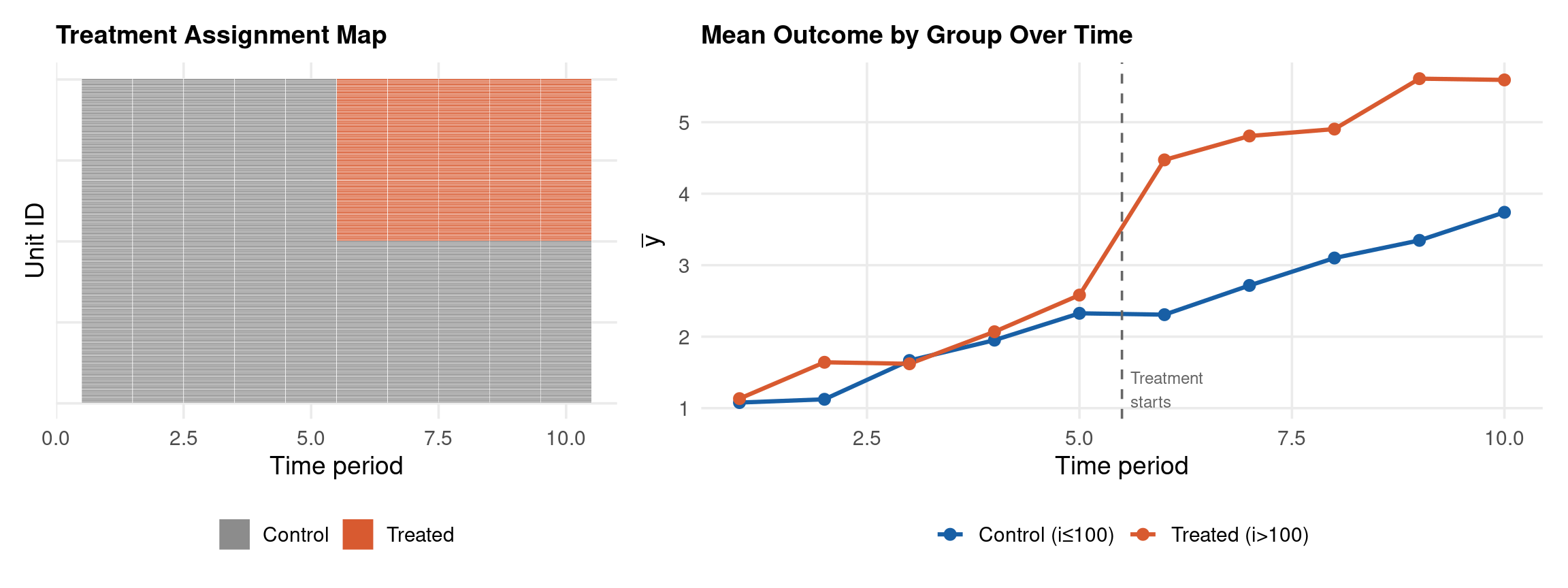
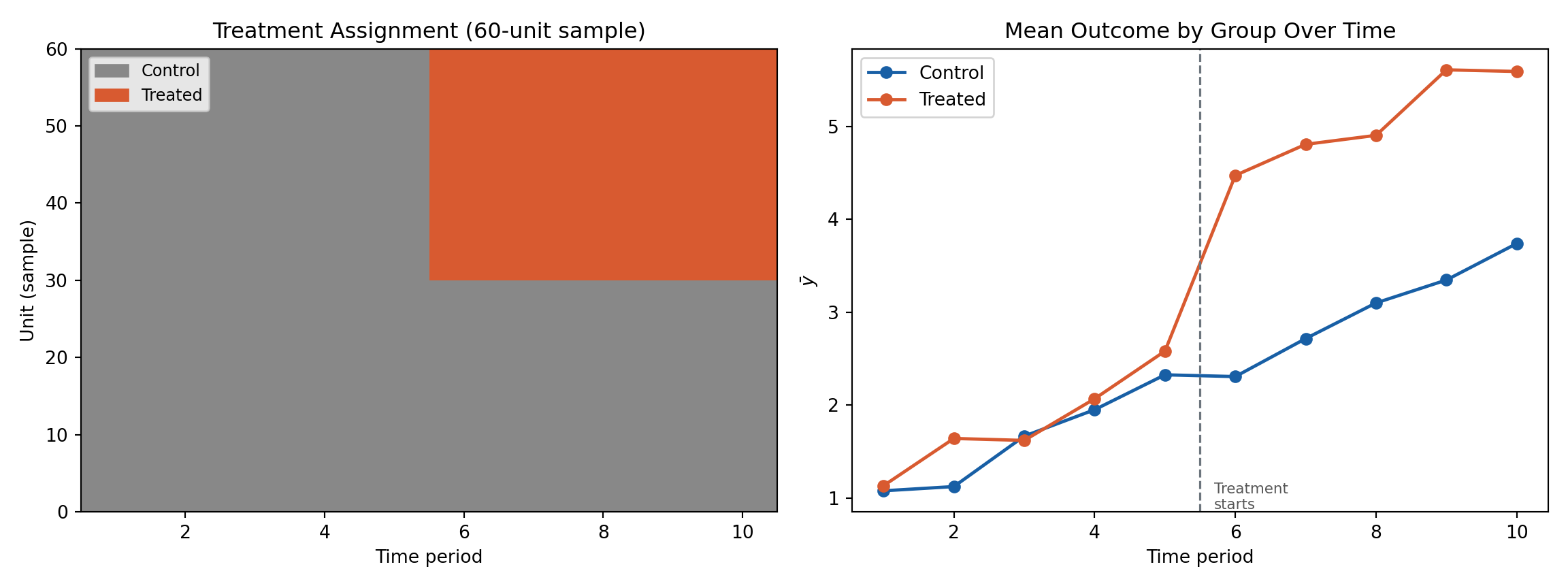
Units \(i = 101\)–\(200\) are treated starting at \(t = 6\) (a clean simultaneous treatment for the main DGP). A staggered variant is generated separately for the variations section.

DGP — Code Implementation

set.seed(14159)
N <- 200; Tper <- 10
beta_d <- 2.0; gamma1 <- 1.5; gamma2 <- 0.8
sigma_eps <- 0.5; rho <- 0.5

alpha_i <- rnorm(N, 0, 1)

panel <- tibble(id = 1:N, alpha = alpha_i) %>%
  crossing(time = 1:Tper) %>%
  arrange(id, time) %>%
  mutate(
    lambda      = 0.3 * time,
    x1          = rho * alpha + sqrt(1 - rho^2) * rnorm(n()),
    x2          = rnorm(n(), 1, 1),
    eps         = rnorm(n(), 0, sigma_eps),
    treat       = as.integer(id > 100 & time >= 6),
    y           = alpha + lambda + beta_d * treat + gamma1 * x1 + gamma2 * x2 + eps,
    first_treat = case_when(id > 150 ~ 7L, id > 100 ~ 4L, TRUE ~ 0L)
  ) %>%
  select(id, time, y, x1, x2, treat, first_treat)

import numpy as np
import pandas as pd

np.random.seed(14159)
N, T = 200, 10
beta_d, gamma1, gamma2 = 2.0, 1.5, 0.8
sigma_eps, rho = 0.5, 0.5

ids      = np.repeat(np.arange(1, N+1), T)
times    = np.tile(np.arange(1, T+1), N)
alpha_i  = np.random.normal(0, 1, N)
alpha    = np.repeat(alpha_i, T)
lam      = 0.3 * times
x1       = rho * alpha + np.sqrt(1 - rho**2) * np.random.normal(0, 1, N*T)
x2       = np.random.normal(1, 1, N*T)
eps      = np.random.normal(0, sigma_eps, N*T)
treat    = ((ids > 100) & (times >= 6)).astype(int)
y        = alpha + lam + beta_d*treat + gamma1*x1 + gamma2*x2 + eps
first_t  = np.where(ids > 150, 7, np.where(ids > 100, 4, 0))

panel = pd.DataFrame({"id": ids, "time": times, "y": y,
                      "x1": x1, "x2": x2, "treat": treat,
                      "first_treat": first_t})

* --- Stata DGP (reference code; data provided by panel-TWFE-DGP.R) ---
clear
set seed 14159
set obs 200

gen id      = _n
gen alpha_i = rnormal(0, 1)

expand 10
bysort id: gen time = _n

gen lambda      = 0.3 * time
gen x1          = 0.5 * alpha_i + sqrt(0.75) * rnormal()
gen x2          = rnormal(1, 1)
gen eps         = rnormal(0, 0.5)
gen treat       = (id > 100 & time >= 6)
gen y           = alpha_i + lambda + 2.0*treat + 1.5*x1 + 0.8*x2 + eps
gen first_treat = cond(id>150, 7, cond(id>100, 4, 0))

keep id time y x1 x2 treat first_treat
xtset id time

Data Preview

df %>%
  arrange(id, time) %>%
  slice_head(n = 12) %>%
  kbl(digits = 3,
      caption = "panel-TWFE.csv — first 12 rows") %>%
  kable_styling(font_size = 18, full_width = FALSE)

panel-TWFE.csv — first 12 rows

id	time	y	x1	x2	treat	first_treat
1	1	1.556	-0.128	0.836	0	0
1	2	1.564	-0.306	0.769	0	0
1	3	0.844	0.769	-0.643	0	0
1	4	4.484	0.352	3.725	0	0
1	5	6.993	2.851	0.476	0	0
1	6	4.086	0.172	1.300	0	0
1	7	2.339	-0.277	0.815	0	0
1	8	5.090	0.510	1.645	0	0
1	9	6.892	0.653	1.968	0	0
1	10	7.556	1.123	2.270	0	0
2	1	2.381	0.466	1.731	0	0
2	2	1.835	0.278	1.699	0	0

import pandas as pd

df_py = pd.read_csv("../data/panel-TWFE.csv")
print(df_py.head(12).to_string(index=False))

 id  time        y        x1        x2  treat  first_treat
  1     1 1.555582 -0.128465  0.835635      0            0
  1     2 1.563685 -0.305758  0.768940      0            0
  1     3 0.844416  0.768877 -0.643014      0            0
  1     4 4.484330  0.352153  3.724672      0            0
  1     5 6.993028  2.850507  0.475590      0            0
  1     6 4.085653  0.172200  1.299745      0            0
  1     7 2.338834 -0.277084  0.814764      0            0
  1     8 5.090221  0.510105  1.645039      0            0
  1     9 6.892408  0.652856  1.968249      0            0
  1    10 7.556255  1.123250  2.269553      0            0
  2     1 2.381473  0.465657  1.731155      0            0
  2     2 1.835480  0.278443  1.698534      0            0

print(f"\nShape: {df_py.shape[0]} obs x {df_py.shape[1]} variables")

Shape: 2000 obs x 7 variables

print(f"Treated obs      : {df_py['treat'].sum()}  ({df_py['treat'].mean()*100:.1f}%)")

Treated obs      : 500  (25.0%)

print(f"Never-treated    : {(df_py.groupby('id')['treat'].max()==0).sum()} units")

Never-treated    : 100 units

quietly import delimited "../data/panel-TWFE.csv", clear
quietly destring _all, replace
quietly xtset id time
list id time y x1 x2 treat first_treat in 1/12, sep(0) noobs
xtdescribe

  | id   time          y          x1          x2   treat   first_~t |
  |-----------------------------------------------------------------|
  |  1      1   1.555583    -.128465    .8356345       0          0 |
  |  1      2   1.563685   -.3057577    .7689398       0          0 |
  |  1      3   .8444158     .768877   -.6430139       0          0 |
  |  1      4    4.48433    .3521526    3.724672       0          0 |
  |  1      5   6.993028    2.850507    .4755899       0          0 |
  |  1      6   4.085653    .1721997    1.299745       0          0 |
  |  1      7   2.338834   -.2770836    .8147643       0          0 |
  |  1      8   5.090221    .5101053    1.645039       0          0 |
  |  1      9   6.892408    .6528559    1.968249       0          0 |
  |  1     10   7.556255     1.12325    2.269553       0          0 |
  |  2      1   2.381473    .4656573    1.731155       0          0 |
  |  2      2   1.835479    .2784433    1.698534       0          0 |
  +-----------------------------------------------------------------+

      id:  1, 2, ..., 200                                    n =        200
    time:  1, 2, ..., 10                                     T =         10
           Delta(time) = 1 unit
           Span(time)  = 10 periods
           (id*time uniquely identifies each observation)

Distribution of T_i:   min      5%     25%       50%       75%     95%     max
                        10      10      10        10        10      10      10

     Freq.  Percent    Cum. |  Pattern
 ---------------------------+------------
      200    100.00  100.00 |  1111111111
 ---------------------------+------------
      200    100.00         |  XXXXXXXXXX

DGP — Diagnostics

# Plot 1: treatment map
p_treat <- df %>%
  mutate(treated = factor(treat, labels = c("Control", "Treated")),
         id_grp  = cut(id, breaks = c(0,50,100,150,200),
                       labels = c("G1 (1-50)","G2 (51-100)","G3 (101-150)","G4 (151-200)"))) %>%
  ggplot(aes(x = time, y = id, fill = treated)) +
  geom_tile(colour = "white", linewidth = 0.15) +
  scale_fill_manual(values = c("Control" = col_muted, "Treated" = col_accent)) +
  labs(title = "Treatment Assignment", x = "Time period", y = "Unit ID", fill = NULL) +
  theme(legend.position = "right", axis.text.y = element_blank())

# Plot 2: mean outcome by group × time
p_trends <- df %>%
  mutate(Group = if_else(id > 100, "Treated (i>100)", "Control (i≤100)")) %>%
  group_by(Group, time) %>%
  summarise(mean_y = mean(y), .groups = "drop") %>%
  ggplot(aes(x = time, y = mean_y, colour = Group, group = Group)) +
  geom_line(linewidth = 1.1) + geom_point(size = 2.5) +
  geom_vline(xintercept = 5.5, linetype = "dashed", colour = "grey40") +
  annotate("text", x = 5.6, y = Inf, label = "Treatment starts", hjust = 0,
           vjust = 1.5, size = 3.5, colour = "grey40") +
  scale_colour_manual(values = c("Control (i≤100)" = col_main,
                                 "Treated (i>100)" = col_accent)) +
  labs(title = "Mean Outcome by Group Over Time",
       x = "Time period", y = "Mean y", colour = NULL)

p_treat + p_trends + plot_layout(widths = c(1, 1.5))

import pandas as pd
import numpy as np
import matplotlib.pyplot as plt
import matplotlib.patches as mpatches

df_py2 = pd.read_csv("../data/panel-TWFE.csv")

fig, axes = plt.subplots(1, 2, figsize=(12, 4.5))

# Treatment map (sample of 60 units for clarity)
sample_ids = list(range(1, 31)) + list(range(101, 131))
sub = df_py2[df_py2["id"].isin(sample_ids)]
pivot_treat = sub.pivot(index="id", columns="time", values="treat")
from matplotlib.colors import ListedColormap
cmap = ListedColormap(["#888888", "#D85A30"])
axes[0].imshow(pivot_treat.values, aspect="auto", cmap=cmap, origin="lower",
               extent=[0.5, 10.5, 0, len(sample_ids)])
axes[0].set_xlabel("Time period"); axes[0].set_ylabel("Unit (sample)");
axes[0].set_title("Treatment Assignment (60-unit sample)");
patches = [mpatches.Patch(color="#888888", label="Control"),
           mpatches.Patch(color="#D85A30", label="Treated")]
axes[0].legend(handles=patches, loc="upper left", fontsize=9);

# Mean outcome by group
for sub_df, col, lbl in [(df_py2[df_py2.id <= 100], "#185FA5", "Control"),
                          (df_py2[df_py2.id > 100],  "#D85A30", "Treated")]:
    mn = sub_df.groupby("time")["y"].mean()
    axes[1].plot(mn.index, mn.values, marker="o", color=col, linewidth=1.8, label=lbl);
axes[1].axvline(5.5, linestyle="--", color="#6c757d", linewidth=1.2);
axes[1].text(5.7, axes[1].get_ylim()[0], "Treatment\nstarts", fontsize=8,
             color="#555", va="bottom");
axes[1].set_xlabel("Time period"); axes[1].set_ylabel(r"$\bar{y}$");
axes[1].set_title("Mean Outcome by Group Over Time");
axes[1].legend(fontsize=10, loc="upper left", framealpha=0.85);
plt.tight_layout()
plt.show()

quietly import delimited "../data/panel-TWFE.csv", clear
quietly destring _all, replace
quietly xtset id time
gen grp = (id > 100)
preserve
collapse (mean) mean_y = y, by(grp time)
twoway (line mean_y time if grp == 0, lcolor(navy) lpattern(solid) lwidth(medthick)) ///
       (line mean_y time if grp == 1, lcolor(orange_red) lpattern(solid) lwidth(medthick)), ///
    xline(5.5, lpattern(dash) lcolor(gray)) ///
    legend(order(1 "Control (i{&le}100)" 2 "Treated (i>100)") rows(1)) ///
    title("Mean Outcome by Group Over Time") ///
    xtitle("Time period") ytitle("Mean y") xlabel(1(1)10)
cap mkdir plots
 quietly graph export "../plots/dgp-diag-stata.png", replace width(800)
restore

Required Libraries

library(AER)          # auto-loads sandwich, lmtest, car
library(sandwich)     # vcovCL, vcovHC — clustered/robust SEs
library(lmtest)       # coeftest, pbgtest — serial correlation
library(plm)          # plm(), pFtest(), plmtest(), pcdtest()
library(fixest)       # feols() — fast TWFE with any FE dimensions
library(did)          # Callaway & Sant'Anna (2021) staggered DiD
library(bacondecomp)  # bacon() — Goodman-Bacon decomposition
library(modelsummary) # regression tables
library(kableExtra)   # table formatting
library(broom)        # tidy(), glance()
library(tidyverse)
library(patchwork)

import numpy as np                         # numerical computing
import pandas as pd                        # data frames
import statsmodels.api as sm               # OLS, add_constant
from scipy.stats import chi2 as chi2_dist  # chi2 p-values
from scipy.stats import f as f_dist        # F-test p-values
from linearmodels.panel import (           # panel estimators
    PooledOLS, PanelOLS, compare
)
import pyfixest as pf                      # TWFE (mirrors Stata reghdfe)
import wooldridge as woo                   # Wooldridge datasets
import matplotlib.pyplot as plt
import warnings; warnings.filterwarnings("ignore")
print("All packages loaded.")

All packages loaded.

* --- Built-in XT commands ---
* xtset       – declare panel structure
* xtreg       – entity/time FE via LSDV
* xtsum       – within/between summary statistics
* xttest0     – Breusch-Pagan LM test (after xtreg, re)

* --- User-written (install once) ---
* ssc install ftools,      replace   // reghdfe dependency
* ssc install require,     replace   // reghdfe meta-dependency manager
* ssc install reghdfe,     replace   // fast TWFE (absorbs high-dim FE)
* ssc install estout,      replace   // esttab, eststo, estadd tables
* ssc install xttest3,     replace   // Modified Wald for heteroskedasticity
* ssc install xtcd2,       replace   // Pesaran cross-sectional dependence
* ssc install bacondecomp, replace   // Goodman-Bacon decomposition
* ssc install csdid,       replace   // Callaway & Sant'Anna staggered DiD
* ssc install drdid,       replace   // Doubly-robust DiD (Sant'Anna & Zhao 2020)
* ssc install coefplot,    replace   // coefficient plots / event study plots

Load Data & Descriptive Statistics

df  <- read_csv("../data/panel-TWFE.csv")
pdf <- pdata.frame(df, index = c("id", "time"))
df %>% select(y, x1, x2, treat) %>% summary()

       y                 x1                 x2              treat     
 Min.   :-4.7526   Min.   :-2.88543   Min.   :-2.1136   Min.   :0.00  
 1st Qu.: 0.9389   1st Qu.:-0.73883   1st Qu.: 0.3103   1st Qu.:0.00  
 Median : 2.8127   Median :-0.05318   Median : 1.0169   Median :0.00  
 Mean   : 2.8894   Mean   :-0.04736   Mean   : 1.0158   Mean   :0.25  
 3rd Qu.: 4.7264   3rd Qu.: 0.63008   3rd Qu.: 1.6962   3rd Qu.:0.25  
 Max.   :13.2553   Max.   : 3.17948   Max.   : 4.9439   Max.   :1.00  

df_py = pd.read_csv("../data/panel-TWFE.csv")
df_py_idx = df_py.set_index(["id", "time"])
print(df_py.describe().round(4))

              id      time          y  ...         x2      treat  first_treat
count  2000.0000  2000.000  2000.0000  ...  2000.0000  2000.0000    2000.0000
mean    100.5000     5.500     2.8894  ...     1.0158     0.2500       2.7500
std      57.7487     2.873     2.7893  ...     1.0100     0.4331       2.9482
min       1.0000     1.000    -4.7526  ...    -2.1136     0.0000       0.0000
25%      50.7500     3.000     0.9389  ...     0.3103     0.0000       0.0000
50%     100.5000     5.500     2.8127  ...     1.0169     0.0000       2.0000
75%     150.2500     8.000     4.7264  ...     1.6962     0.2500       4.7500
max     200.0000    10.000    13.2553  ...     4.9439     1.0000       7.0000

[8 rows x 7 columns]

quietly import delimited "../data/panel-TWFE.csv", clear
quietly destring _all, replace
quietly xtset id time
xtsum y x1 x2 treat

Variable         |      Mean   Std. dev.       Min        Max |    Observations
-----------------+--------------------------------------------+----------------
y        overall |   2.88943   2.789264  -4.752584   13.25526 |     N =    2000
         between |             1.902014  -1.630829   8.215165 |     n =     200
         within  |             2.044168  -3.932627   8.900282 |     T =      10
                 |                                            |
x1       overall | -.0473601   1.008786  -2.885428    3.17948 |     N =    2000
         between |             .5717692  -1.385513   1.460393 |     n =     200
         within  |             .8319861  -2.650447   2.885352 |     T =      10
                 |                                            |
x2       overall |  1.015845    1.01005  -2.113644   4.943884 |     N =    2000
         between |             .2940984   .0943723   1.953338 |     n =     200
         within  |             .9664866  -1.925585   4.790418 |     T =      10
                 |                                            |
treat    overall |       .25    .433121          0          1 |     N =    2000
         between |             .2506274          0         .5 |     n =     200
         within  |             .3536418       -.25        .75 |     T =      10

TWFE Estimation

# Pooled OLS (biased — ignores both alpha_i and lambda_t)
ols_r  <- lm(y ~ x1 + x2 + treat, data = df)

# Entity FE only (via within demeaning; time shocks still omitted)
fe_r   <- plm(y ~ x1 + x2 + treat, data = pdf, model = "within", effect = "individual")

# Two-Way FE — the recommended estimator
twfe_r <- feols(y ~ x1 + x2 + treat | id + time, data = df, cluster = ~id)

summary(twfe_r)

OLS estimation, Dep. Var.: y
Observations: 2,000
Fixed-effects: id: 200,  time: 10
Standard-errors: Clustered (id) 
      Estimate Std. Error  t value  Pr(>|t|)    
x1    1.528639   0.013178 115.9969 < 2.2e-16 ***
x2    0.808486   0.011982  67.4729 < 2.2e-16 ***
treat 1.933068   0.046524  41.5498 < 2.2e-16 ***
---
Signif. codes:  0 '***' 0.001 '**' 0.01 '*' 0.05 '.' 0.1 ' ' 1
RMSE: 0.474853     Adj. R2: 0.967581
                 Within R2: 0.912852

# Pooled OLS
exog_c = sm.add_constant(df_py_idx[["x1","x2","treat"]])
ols_py = PooledOLS(df_py_idx["y"], exog_c).fit(cov_type="unadjusted")

# Entity FE only
fe_py  = PanelOLS(df_py_idx["y"], df_py_idx[["x1","x2","treat"]],
                  entity_effects=True).fit(cov_type="unadjusted")

# Two-Way FE via pyfixest (mirrors reghdfe)
twfe_py = pf.feols("y ~ x1 + x2 + treat | id + time",
                   data=df_py, vcov={"CRV1": "id"})
twfe_py.summary()

###

Estimation:  OLS
Dep. var.: y, Fixed effects: id + time
sample: None = all
Inference:  CRV1
Observations:  2000

| Coefficient   |   Estimate |   Std. Error |   t value |   Pr(>|t|) |   2.5% |   97.5% |
|:--------------|-----------:|-------------:|----------:|-----------:|-------:|--------:|
| x1            |      1.529 |        0.013 |   115.997 |      0.000 |  1.503 |   1.555 |
| x2            |      0.808 |        0.012 |    67.473 |      0.000 |  0.785 |   0.832 |
| treat         |      1.933 |        0.047 |    41.550 |      0.000 |  1.841 |   2.025 |
---
RMSE: 0.475 R2: 0.971 R2 Within: 0.913 

quietly import delimited "../data/panel-TWFE.csv", clear
quietly destring _all, replace
quietly xtset id time

* Pooled OLS
quietly regress y x1 x2 treat
estimates store OLS

* Entity FE only
quietly xtreg y x1 x2 treat, fe
estimates store FE_entity

* Two-Way FE via reghdfe (absorbs id + time simultaneously)
cap ssc install require, replace
reghdfe y x1 x2 treat, absorb(id time) vce(cluster id)
estimates store TWFE

(MWFE estimator converged in 2 iterations)

HDFE Linear regression                            Number of obs   =      2,000
Absorbing 2 HDFE groups                           F(   3,    199) =    7218.58
Statistics robust to heteroskedasticity           Prob > F        =     0.0000
                                                  R-squared       =     0.9710
                                                  Adj R-squared   =     0.9676
                                                  Within R-sq.    =     0.9129
Number of clusters (id)      =        200         Root MSE        =     0.5022

                                   (Std. err. adjusted for 200 clusters in id)
------------------------------------------------------------------------------
             |               Robust
           y | Coefficient  std. err.      t    P>|t|     [95% conf. interval]
-------------+----------------------------------------------------------------
          x1 |   1.528639   .0131783   116.00   0.000     1.502652    1.554626
          x2 |    .808486   .0119824    67.47   0.000     .7848572    .8321147
       treat |   1.933068   .0465241    41.55   0.000     1.841325    2.024812
       _cons |   1.657263   .0156138   106.14   0.000     1.626473    1.688053
------------------------------------------------------------------------------

Absorbed degrees of freedom:
-----------------------------------------------------+
 Absorbed FE | Categories  - Redundant  = Num. Coefs |
-------------+---------------------------------------|
          id |       200         200           0    *|
        time |        10           1           9     |
-----------------------------------------------------+
* = FE nested within cluster; treated as redundant for DoF computation

True vs Estimated — Equation Format

• Equation
• Note
• Tip

\[\underbrace{y_{it} = \alpha_i + 0.3t + \mathbf{2.000}\,D_{it} + \mathbf{1.500}\,x_{1,it} + \mathbf{0.800}\,x_{2,it} + \varepsilon_{it}}_{\text{True DGP}}\]

\[\hat{y}_{it}^{OLS} = \underset{}{3.027}\,D_{it} + \underset{}{2}\,x_{1,it} + \underset{}{0.781}\,x_{2,it}\]

\[\hat{y}_{it}^{FE\text{(entity)}} = \underset{}{3.474}\,D_{it} + \underset{}{1.521}\,x_{1,it} + \underset{}{0.791}\,x_{2,it}\]

\[\hat{y}_{it}^{TWFE\,\star} = \underset{}{1.933}\,D_{it} + \underset{}{1.529}\,x_{1,it} + \underset{}{0.808}\,x_{2,it}\]

\(\star\) Consistent estimator

Why does entity FE alone fail?

Time effects \(\lambda_t = 0.3t\) are omitted. Since treatment turns on at \(t \geq 6\) (high-\(\lambda_t\) periods), entity-only FE confounds the time trend with the treatment effect.

\[\hat{\beta}^{FE(entity)} \approx \beta + \underbrace{\frac{\text{Cov}(\tilde{D}_{it},\, \lambda_t)}{\text{Var}(\tilde{D}_{it})}}_{\text{omitted-variable bias} > 0} \implies \hat{\beta}^{FE} > \beta^{true} = 2.0\]

Why does TWFE recover the truth?

Entity FE removes \(\alpha_i\); time FE removes \(\lambda_t\). The double-demeaned treatment \(\ddot{D}_{it}\) is orthogonal to both fixed effects by construction:

\[\mathbb{E}[\ddot{D}_{it}\, \alpha_i] = 0 \quad \text{and} \quad \mathbb{E}[\ddot{D}_{it}\, \lambda_t] = 0\]

\[\implies \hat{\beta}^{TWFE} \xrightarrow{p} \beta = 2.0 \quad \checkmark\]

Results — Tabular Format

• Results
• LaTeX

modelsummary(
  list("Pooled OLS" = ols_r, "Entity FE" = fe_r, "Two-Way FE" = twfe_r),
  coef_map  = c("treat" = "Treatment (D)",
                "x1"    = "x₁ (endogenous)",
                "x2"    = "x₂ (exogenous)"),
  stars     = TRUE,
  gof_omit  = "IC|Log|RMSE",
  notes     = "Clustered SEs (by id) for TWFE. *** p<0.01, ** p<0.05, * p<0.1",
  title     = "Simulation: OLS vs Entity FE vs Two-Way FE"
)

Simulation: OLS vs Entity FE vs Two-Way FE

	Pooled OLS	Entity FE	Two-Way FE
+ p < 0.1, * p < 0.05, ** p < 0.01, *** p < 0.001
Clustered SEs (by id) for TWFE. *** p<0.01, ** p<0.05, * p<0.1
Treatment (D)	3.027***	3.474***	1.933***
	(0.066)	(0.057)	(0.047)
x₁ (endogenous)	2.000***	1.521***	1.529***
	(0.028)	(0.024)	(0.013)
x₂ (exogenous)	0.781***	0.791***	0.808***
	(0.028)	(0.021)	(0.012)
Num.Obs.	2000	2000	2000
R2	0.793	0.826	0.971
R2 Adj.	0.793	0.806	0.968
R2 Within			0.913
R2 Within Adj.			0.913
F	2556.150
FE: id			X
FE: time			X

tbl_latex <- modelsummary(
  list("Pooled OLS" = ols_r, "Entity FE" = fe_r, "Two-Way FE" = twfe_r),
  coef_map = c("treat" = "Treatment ($D$)", "x1" = "$x_1$", "x2" = "$x_2$"),
  stars    = TRUE,
  gof_omit = "IC|Log|RMSE",
  output   = "latex"
)
writeLines(as.character(tbl_latex))

\begin{table}
\centering
\begin{talltblr}[         %% tabularray outer open
entry=none,label=none,
note{}={+ p \num{< 0.1}, * p \num{< 0.05}, ** p \num{< 0.01}, *** p \num{< 0.001}},
]                     %% tabularray outer close
{                     %% tabularray inner open
colspec={Q[]Q[]Q[]Q[]},
hline{2}={1-4}{solid, black, 0.05em},
hline{8}={1-4}{solid, black, 0.05em},
hline{1}={1-4}{solid, black, 0.08em},
hline{16}={1-4}{solid, black, 0.08em},
column{2-4}={}{halign=c},
column{1}={}{halign=l},
}                     %% tabularray inner close
& Pooled OLS & Entity FE & Two-Way FE \\
Treatment (\$D\$) & \num{3.027}*** & \num{3.474}*** & \num{1.933}*** \\
& (\num{0.066}) & (\num{0.057}) & (\num{0.047}) \\
\$x\_1\$ & \num{2.000}*** & \num{1.521}*** & \num{1.529}*** \\
& (\num{0.028}) & (\num{0.024}) & (\num{0.013}) \\
\$x\_2\$ & \num{0.781}*** & \num{0.791}*** & \num{0.808}*** \\
& (\num{0.028}) & (\num{0.021}) & (\num{0.012}) \\
Num.Obs. & \num{2000} & \num{2000} & \num{2000} \\
R2 & \num{0.793} & \num{0.826} & \num{0.971} \\
R2 Adj. & \num{0.793} & \num{0.806} & \num{0.968} \\
R2 Within &  &  & \num{0.913} \\
R2 Within Adj. &  &  & \num{0.913} \\
F & \num{2556.150} &  &  \\
FE: id &  &  & X \\
FE: time &  &  & X \\
\end{talltblr}
\end{table}

library(modelsummary)
modelsummary(
  list("Pooled OLS" = ols_r, "Entity FE" = fe_r, "Two-Way FE" = twfe_r),
  coef_map = c("treat"="Treatment (D)", "x1"="x1", "x2"="x2"),
  stars = TRUE, gof_omit = "IC|Log|RMSE",
  title = "Simulation: OLS vs Entity FE vs Two-Way FE"
)

m1 = pf.feols("y ~ x1 + x2 + treat",            data=df_py)
m2 = pf.feols("y ~ x1 + x2 + treat | id",        data=df_py)
m3 = pf.feols("y ~ x1 + x2 + treat | id + time", data=df_py, vcov={"CRV1": "id"})

def _stars(p):
    return "***" if p < .01 else "**" if p < .05 else "*" if p < .10 else ""

var_labels = {"treat": "Treatment (D)", "x1": "x\u2081", "x2": "x\u2082"}
models     = [("Pooled OLS", m1), ("Entity FE", m2), ("TWFE", m3)]
col_w      = 16

header = f"{'':22}" + "".join(f"{nm:>{col_w}}" for nm, _ in models)
sep    = "-" * len(header)
print(header); print(sep)

                            Pooled OLS       Entity FE            TWFE
----------------------------------------------------------------------

for v, lbl in var_labels.items():
    row_c = f"{lbl:<22}"
    row_s = f"{'':22}"
    for _, m in models:
        c, s, p = m.coef(), m.se(), m.pvalue()
        if v in c.index:
            row_c += f"{c[v]:>10.4f}{_stars(p[v]):>6}"
            row_s += f"({'(' + f'{s[v]:.4f}' + ')':>14}"
        else:
            row_c += f"{'—':>{col_w}}"
            row_s += f"{'':>{col_w}}"
    print(row_c); print(row_s)

Treatment (D)             3.0267   ***    3.4736   ***    1.9331   ***
                      (      (0.0655)(      (0.0570)(      (0.0465)
x₁                        2.0005   ***    1.5213   ***    1.5286   ***
                      (      (0.0281)(      (0.0243)(      (0.0132)
x₂                        0.7808   ***    0.7909   ***    0.8085   ***
                      (      (0.0281)(      (0.0209)(      (0.0120)

print(sep)

----------------------------------------------------------------------

print(f"{'N':22}" + "".join(f"{len(m.resid()):>{col_w}}" for _, m in models))

N                                 2000            2000            2000

print(f"{'Entity FE':22}" + "".join(f"{'No' if i==0 else 'Yes':>{col_w}}" for i in range(3)))

Entity FE                           No             Yes             Yes

print(f"{'Time FE':22}" + "".join(f"{'No' if i<2 else 'Yes':>{col_w}}" for i in range(3)))

Time FE                             No              No             Yes

print("\n* p<0.10  ** p<0.05  *** p<0.01")

* p<0.10  ** p<0.05  *** p<0.01

quietly import delimited "../data/panel-TWFE.csv", clear
quietly destring _all, replace
quietly xtset id time
quietly regress y x1 x2 treat
quietly estimates store OLS
quietly xtreg y x1 x2 treat, fe
quietly estimates store FE_entity
cap ssc install require, replace
quietly reghdfe y x1 x2 treat, absorb(id time) vce(cluster id)
quietly estimates store TWFE
esttab OLS FE_entity TWFE,                                      ///
    b(4) se(4) star(* 0.10 ** 0.05 *** 0.01)                   ///
    keep(treat x1 x2)                                           ///
    stats(N r2, fmt(0 3) labels("N" "R²"))                      ///
    mtitles("Pooled OLS" "Entity FE" "Two-Way FE")              ///
    title("Simulation: OLS vs Entity FE vs Two-Way FE")

Simulation: OLS vs Entity FE vs Two-Way FE
------------------------------------------------------------
                      (1)             (2)             (3)   
               Pooled OLS       Entity FE      Two-Way FE   
------------------------------------------------------------
x1                 2.0005***       1.5213***       1.5286***
                 (0.0281)        (0.0243)        (0.0132)   

x2                 0.7808***       0.7909***       0.8085***
                 (0.0281)        (0.0209)        (0.0120)   

treat              3.0267***       3.4736***       1.9331***
                 (0.0655)        (0.0570)        (0.0465)   
------------------------------------------------------------
N                    2000            2000            2000   
R²                  0.793           0.826           0.971   
------------------------------------------------------------
Standard errors in parentheses
* p<0.10, ** p<0.05, *** p<0.01

F-test for Entity Fixed Effects — Theory

Null hypothesis: all entity effects are jointly zero (pooled OLS suffices)

\[H_0: \alpha_1 = \alpha_2 = \cdots = \alpha_N = 0\]

\[F_{entity} = \frac{(RSS_{OLS} - RSS_{FE})\,/\,(N-1)}{RSS_{FE}\,/\,(NT - N - k)} \;\sim\; F(N-1,\; NT-N-k)\]

Component	Meaning
\(RSS_{OLS}\)	Residual sum of squares from pooled OLS
\(RSS_{FE}\)	Residual sum of squares from entity FE
\(N - 1\)	Numerator df (entity dummies less one)
\(NT - N - k\)	Denominator df

Reject when: \(p\)-value \(< 0.05\) — entity effects are jointly significant; prefer FE over pooled OLS.

F-test for Entity Fixed Effects — Code

pFtest(fe_r, lm(y ~ x1 + x2 + treat, data = df))

    F test for individual effects

data:  y ~ x1 + x2 + treat
F = 10.872, df1 = 199, df2 = 1797, p-value < 2.2e-16
alternative hypothesis: significant effects

fe_py2 = PanelOLS(df_py_idx["y"], df_py_idx[["x1","x2","treat"]],
                  entity_effects=True).fit(cov_type="unadjusted")
resid_fe  = fe_py2.resids.to_numpy().ravel()
ols_py2   = PooledOLS(df_py_idx["y"],
                      sm.add_constant(df_py_idx[["x1","x2","treat"]])).fit()
resid_ols = (df_py_idx["y"].to_numpy() -
             ols_py2.fitted_values.to_numpy()).ravel()
N_i, T_i, k_i = 200, 10, 3; NT_i = N_i * T_i
RSS_fe  = float(np.dot(resid_fe,  resid_fe))
RSS_ols = float(np.dot(resid_ols, resid_ols))
F_ent   = ((RSS_ols - RSS_fe)/(N_i-1)) / (RSS_fe/(NT_i-N_i-k_i))
p_ent   = float(1 - f_dist.cdf(F_ent, N_i-1, NT_i-N_i-k_i))
print(f"F({N_i-1}, {NT_i-N_i-k_i}) = {F_ent:.4f},  p = {p_ent:.3e}")

F(199, 1797) = 345648.0561,  p = 1.110e-16

print("Decision:", "Reject H₀ → entity FE significant" if p_ent < 0.05 else "Do not reject")

Decision: Reject H₀ → entity FE significant

quietly import delimited "../data/panel-TWFE.csv", clear
quietly destring _all, replace
quietly xtset id time
* F-test appears automatically in xtreg, fe output
xtreg y x1 x2 treat, fe
* "F test that all u_i=0: F(N-1, NT-N-k)  Prob > F"

Fixed-effects (within) regression               Number of obs     =      2,000
Group variable: id                              Number of groups  =        200

R-squared:                                      Obs per group:
     Within  = 0.8255                                         min =         10
     Between = 0.7111                                         avg =       10.0
     Overall = 0.7627                                         max =         10

                                                F(3, 1797)        =    2834.27
corr(u_i, Xb) = 0.1757                          Prob > F          =     0.0000

------------------------------------------------------------------------------
           y | Coefficient  Std. err.      t    P>|t|     [95% conf. interval]
-------------+----------------------------------------------------------------
          x1 |   1.521264   .0242593    62.71   0.000     1.473684    1.568843
          x2 |    .790903   .0208534    37.93   0.000     .7500035    .8318026
       treat |   3.473628   .0570404    60.90   0.000     3.361756    3.585501
       _cons |   1.289635   .0325642    39.60   0.000     1.225767    1.353503
-------------+----------------------------------------------------------------
     sigma_u |  1.0760798
     sigma_e |   .9005519
         rho |  .58810673   (fraction of variance due to u_i)
------------------------------------------------------------------------------
F test that all u_i=0: F(199, 1797) = 10.87                  Prob > F = 0.0000

F-test for Time Fixed Effects — Theory

Null hypothesis: all time effects are jointly zero (entity-only FE suffices)

\[H_0: \lambda_1 = \lambda_2 = \cdots = \lambda_T = 0\]

\[F_{time} = \frac{(RSS_{FE_{entity}} - RSS_{TWFE})\,/\,(T-1)}{RSS_{TWFE}\,/\,(NT - N - T - k + 1)} \;\sim\; F(T-1,\; NT-N-T-k+1)\]

Component	Meaning
\(RSS_{FE_{entity}}\)	RSS from entity FE only
\(RSS_{TWFE}\)	RSS from TWFE (entity + time FE)
\(T - 1\)	Numerator df (time dummies less one)

Reject when: \(p\)-value \(< 0.05\) — time effects are jointly significant; use TWFE, not entity-only FE.

Warning

Presence of significant time effects does not by itself imply violation of parallel trends — it means the common time trend is non-trivial and must be controlled for.

F-test for Time Fixed Effects — Code

fe_time  <- plm(y ~ x1 + x2 + treat, data = pdf, model = "within", effect = "time")
twfe_plm <- plm(y ~ x1 + x2 + treat, data = pdf, model = "within", effect = "twoways")
pFtest(twfe_plm, fe_r)   # tests whether time FE are jointly significant

    F test for twoways effects

data:  y ~ x1 + x2 + treat
F = 443.34, df1 = 9, df2 = 1788, p-value < 2.2e-16
alternative hypothesis: significant effects

twfe_lm = PanelOLS(df_py_idx["y"], df_py_idx[["x1","x2","treat"]],
                   entity_effects=True, time_effects=True).fit(cov_type="unadjusted")
resid_twfe = twfe_lm.resids.to_numpy().ravel()
N_i, T_i, k_i = 200, 10, 3; NT_i = N_i * T_i
RSS_fe2   = float(np.dot(resid_fe,   resid_fe))
RSS_twfe  = float(np.dot(resid_twfe, resid_twfe))
ddf_num   = T_i - 1
ddf_den   = NT_i - N_i - T_i - k_i + 1
F_time    = ((RSS_fe2 - RSS_twfe)/ddf_num) / (RSS_twfe/ddf_den)
p_time    = float(1 - f_dist.cdf(F_time, ddf_num, ddf_den))
print(f"F({ddf_num}, {ddf_den}) = {F_time:.4f},  p = {p_time:.3e}")

F(9, 1788) = 443.3440,  p = 1.110e-16

print("Decision:", "Reject H₀ → time FE significant → use TWFE" if p_time < 0.05 else "Do not reject")

Decision: Reject H₀ → time FE significant → use TWFE

quietly import delimited "../data/panel-TWFE.csv", clear
quietly destring _all, replace
quietly xtset id time
* Compare entity-only FE vs TWFE via manual F-test (RSS difference)
cap ssc install require, replace
quietly reghdfe y x1 x2 treat, absorb(id)
scalar rss_fe   = e(rss)
scalar df_fe    = e(df_r)
quietly reghdfe y x1 x2 treat, absorb(id time)
scalar rss_twfe = e(rss)
scalar df_twfe  = e(df_r)
* F = [(RSS_fe - RSS_twfe)/(T-1)] / [RSS_twfe / df_twfe]
scalar F_time = ((rss_fe - rss_twfe) / (10 - 1)) / (rss_twfe / df_twfe)
scalar p_time = Ftail(9, df_twfe, F_time)
display "F(9, " df_twfe ") = " %8.4f F_time "   p = " %8.4f p_time
display cond(p_time < 0.05, "Reject H0: time FE significant -> use TWFE", "Cannot reject H0")

F(9, 1788) = 443.3440   p =   0.0000

Reject H0: time FE significant -> use TWFE

Wooldridge Serial Correlation Test — Theory

Wooldridge (2002) proposes a simple test for serial correlation in the idiosyncratic errors \(\varepsilon_{it}\) of a linear panel model; the implementation follows Drukker (2003).

Procedure: estimate the first-differenced equation and test whether residuals \(\Delta\hat{\varepsilon}_{it}\) are serially correlated:

\[H_0: \text{Cov}(\Delta\varepsilon_{it},\, \Delta\varepsilon_{i,t-1}) = 0\]

Under \(H_0\) (no serial correlation), \(\text{Corr}(\Delta\varepsilon_{it}, \Delta\varepsilon_{i,t-1}) = -0.5\).

\[F_{SC} \sim F(1, N-1)\]

The test regresses \(\Delta\hat{\varepsilon}_{it}\) on \(\Delta\hat{\varepsilon}_{i,t-1}\) across units and tests whether the slope equals \(-0.5\).

Reject when: \(p\)-value \(< 0.05\) → serial correlation is present in the idiosyncratic errors → cluster standard errors at the individual level.

Wooldridge Serial Correlation Test — Code

# pbgtest: panel Breusch-Godfrey / Wooldridge-type serial correlation test
pbgtest(twfe_plm, order = 1)

    Breusch-Godfrey/Wooldridge test for serial correlation in panel models

data:  y ~ x1 + x2 + treat
chisq = 17.512, df = 1, p-value = 2.855e-05
alternative hypothesis: serial correlation in idiosyncratic errors

from scipy.stats import t as t_dist

# Step 1: fit TWFE and extract residuals (pyfixest returns a plain numpy array)
twfe_sc  = pf.feols("y ~ x1 + x2 + treat | id + time",
                    data=df_py.sort_values(["id","time"]).reset_index(drop=True))
resid_np = np.asarray(twfe_sc.resid())   # numpy array — no .values needed

# Step 2: attach residuals to a sorted copy of the data
df_sc         = df_py.sort_values(["id","time"]).reset_index(drop=True).copy()
df_sc["e"]    = resid_np

# Step 3: first-difference residuals within each unit
df_sc["de"]   = df_sc.groupby("id")["e"].diff()
df_sc["de_l"] = df_sc.groupby("id")["de"].shift(1)
clean         = df_sc.dropna(subset=["de","de_l"])

# Step 4: OLS of Δε on Δε_{t-1}; test H₀: coef = -0.5
X_sc  = sm.add_constant(clean["de_l"])
sc_m  = sm.OLS(clean["de"], X_sc).fit()
b_sc  = sc_m.params["de_l"]
se_sc = sc_m.bse["de_l"]
t_sc  = (b_sc - (-0.5)) / se_sc
p_sc  = float(2 * (1 - t_dist.cdf(abs(t_sc), df=len(clean) - 2)))

print(f"Coef on lagged \u0394\u03b5 : {b_sc:.4f}   (H\u2080: coef = \u22120.5)")

Coef on lagged Δε : -0.4960   (H₀: coef = −0.5)

print(f"t-stat          : {t_sc:.4f}")

t-stat          : 0.1845

print(f"p-value         : {p_sc:.4f}")

p-value         : 0.8537

print("Decision:", "Reject H\u2080 \u2192 serial correlation present" if p_sc < 0.05
      else "Cannot reject H\u2080")

Decision: Cannot reject H₀

quietly import delimited "../data/panel-TWFE.csv", clear
quietly destring _all, replace
quietly xtset id time
* Wooldridge (2002) test — manual via first differences of TWFE residuals
* Step 1: obtain TWFE residuals using residuals(varname) syntax
cap ssc install require, replace
quietly reghdfe y x1 x2 treat, absorb(id time) residuals(resid_fe)
* Step 2: first-difference the residuals within each unit
quietly by id (time): gen d_resid     = resid_fe - resid_fe[_n-1]
quietly by id (time): gen d_resid_lag = d_resid[_n-1]
* Step 3: regress Δε on Δε_{t-1} and test H0: coef = -0.5
regress d_resid d_resid_lag, cluster(id)
test d_resid_lag = -0.5
* H0: no serial correlation (coef = -0.5 under independence of ε)

Linear regression                               Number of obs     =      1,600
                                                F(1, 199)         =     792.49
                                                Prob > F          =     0.0000
                                                R-squared         =     0.2422
                                                Root MSE          =     .62327

                                   (Std. err. adjusted for 200 clusters in id)
------------------------------------------------------------------------------
             |               Robust
     d_resid | Coefficient  std. err.      t    P>|t|     [95% conf. interval]
-------------+----------------------------------------------------------------
 d_resid_lag |  -.4959515   .0176174   -28.15   0.000    -.5306923   -.4612108
       _cons |   5.22e-10   .0066031     0.00   1.000    -.0130211    .0130211
------------------------------------------------------------------------------


 ( 1)  d_resid_lag = -.5

       F(  1,   199) =    0.05
            Prob > F =    0.8185

Pesaran Cross-Sectional Dependence Test — Theory

In macro/regional panels, idiosyncratic errors may be correlated across units at the same time \(t\) (e.g., due to unobserved common factors). This violates the assumption \(\mathbb{E}[\varepsilon_{it}\varepsilon_{jt}] = 0\) for \(i \neq j\).

This test detects the problem; it does not fix it. The companion deck Spatial Econometrics supplies the remedy — Conley standard errors when dependence decays with distance, and spatial panel models when it is structural.

Pesaran (2004) CD test:

\[CD = \sqrt{\frac{2T}{N(N-1)}} \sum_{i=1}^{N-1}\sum_{j=i+1}^{N} \hat{\rho}_{ij} \;\sim\; \mathcal{N}(0,1)\]

where \(\hat{\rho}_{ij} = \frac{\sum_t \hat{\varepsilon}_{it}\hat{\varepsilon}_{jt}}{\left(\sum_t \hat{\varepsilon}_{it}^2\right)^{1/2}\left(\sum_t \hat{\varepsilon}_{jt}^2\right)^{1/2}}\) is the pair-wise correlation of residuals.

Reject when: \(|CD| > 1.96\) (or \(p < 0.05\)) → cross-sectional dependence is present → consider Driscoll-Kraay standard errors or common correlated effects (CCE) estimator.

Note

In balanced panels with \(T < N\), the CD statistic has good power. For \(T > N\), the LM statistic (\(\sum_{i<j}\hat{\rho}_{ij}^2\)) is preferred.

Pesaran Cross-Sectional Dependence Test — Code

pcdtest(twfe_plm, test = "cd")

    Pesaran CD test for cross-sectional dependence in panels

data:  y ~ x1 + x2 + treat
z = -2.2175, p-value = 0.02659
alternative hypothesis: cross-sectional dependence

# Manual CD test on TWFE residuals
resid_arr = twfe_lm.resids.to_numpy().reshape(200, 10)  # N × T
rhos = []
for i in range(200):
    for j in range(i+1, 200):
        r = np.corrcoef(resid_arr[i], resid_arr[j])[0,1]
        if not np.isnan(r):
            rhos.append(r)
T_i  = 10
CD_stat = np.sqrt(2*T_i / (200*199)) * np.sum(rhos)
from scipy.stats import norm as norm_dist
p_cd = float(2*(1 - norm_dist.cdf(abs(CD_stat))))
print(f"Pesaran CD = {CD_stat:.4f},  p = {p_cd:.4f}")

Pesaran CD = -2.2175,  p = 0.0266

print("Decision:", "Reject H₀ → cross-sectional dependence" if p_cd < 0.05 else "Cannot reject H₀")

Decision: Reject H₀ → cross-sectional dependence

quietly import delimited "../data/panel-TWFE.csv", clear
quietly destring _all, replace
quietly xtset id time
cap ssc install require, replace
quietly reghdfe y x1 x2 treat, absorb(id time) resid
xtcd2, noestimation

Residuals calculated using  predict, residuals.

Testing for weak cross-sectional dependence (CSD)
   H0: weak cross-section dependence
   H1: strong cross-section dependence
------------------------------------------------------------------------
               |    CD            CDw           CDw+          CD*
---------------+--------------------------------------------------------
residuals      |    -2.22       -1.71       6654.12         -2.14
               |  (0.027)     (0.088)       (0.000)       (0.032)
------------------------------------------------------------------------
p-values in parenthesis.
References
  CD:        Pesaran (2015, 2021)
  CDw:       Juodis, Reese (2021)
  CDw+:      CDw with power enhancement from Fan et al. (2015)
  CD*:       Pesaran, Xie (2021) with 4 PC(s)

Heteroskedasticity Test — Theory

Panel models with entity fixed effects may exhibit groupwise heteroskedasticity: \(\text{Var}(\varepsilon_{it}) = \sigma_i^2\) (unit-specific variances).

Modified Wald test (Greene 2000; Wald statistic with unit-specific variance estimates):

\[W = \sum_{i=1}^N \frac{(\hat{\sigma}_i^2 - \hat{\sigma}^2)^2}{\text{Var}(\hat{\sigma}_i^2)} \;\sim\; \chi^2(N)\]

where \(\hat{\sigma}_i^2 = \frac{1}{T}\sum_t \hat{\varepsilon}_{it}^2\) is the within-unit residual variance and \(\hat{\sigma}^2 = \frac{1}{N}\sum_i \hat{\sigma}_i^2\).

Reject when: \(p\)-value \(< 0.05\) → heteroskedastic errors → use heteroskedasticity-robust (or cluster-robust) standard errors.

Tip

In practice, clustering by unit absorbs both serial correlation and heteroskedasticity: vce(cluster id) in Stata; vcov={"CRV1": "id"} in pyfixest; vcovCL(model, cluster=~id) in R.

Heteroskedasticity Test — Code

# Breusch-Pagan test on FE residuals (auxiliary regression of ε² on regressors)
resid_twfe <- residuals(twfe_plm)
df_het     <- df %>% mutate(resid_sq = resid_twfe^2)
bptest(twfe_plm, studentize = FALSE)

    Breusch-Pagan test

data:  twfe_plm
BP = 22.125, df = 3, p-value = 6.143e-05

# Modified Wald: test H0: σ₁² = σ₂² = ... = σ_N²
sigma2_i = np.array([resid_arr[i].var() for i in range(200)])
sigma2   = sigma2_i.mean()
W_wald   = float(200 * np.sum((sigma2_i - sigma2)**2) / (2 * sigma2**2))
p_wald   = float(1 - chi2_dist.cdf(W_wald, df=200))
print(f"Modified Wald χ²(200) = {W_wald:.4f},  p = {p_wald:.4f}")

Modified Wald χ²(200) = 4468.6815,  p = 0.0000

print("Decision:", "Reject H₀ → groupwise heteroskedasticity" if p_wald < 0.05 else "Do not reject H₀")

Decision: Reject H₀ → groupwise heteroskedasticity

quietly import delimited "../data/panel-TWFE.csv", clear
quietly destring _all, replace
quietly xtset id time
quietly xtreg y x1 x2 treat, fe
* Modified Wald test for groupwise heteroskedasticity (xttest3)
xttest3

Modified Wald test for groupwise heteroskedasticity
in fixed effect regression model

H0: sigma(i)^2 = sigma^2 for all i

chi2 (200)  =       2087.60
Prob > chi2 =          0.0000

Test Summary

TWFE Diagnostic Test Results

Test	H0	Statistic	p-value	Decision
F-test: entity FE	All αᵢ = 0	10.872	<2e-16	Reject → entity FE needed
F-test: time FE	All λₜ = 0	443.344	<2e-16	Reject → time FE needed
Serial correlation (BG)	No serial correlation	17.512	2.85e-05	Reject → cluster SEs
Pesaran CD	Cross-sect. independence	-2.218	0.0266	Do not reject → no CD
Heteroskedasticity (BP)	Homoskedasticity	22.125	6.14e-05	Reject → robust SEs

Important

The simulation confirms: both entity and time FEs are necessary, and clustering by unit is warranted. Use feols(... | id + time, cluster = ~id).

Variation: Clustered Standard Errors

OLS/FE SEs assume iid errors. In panels, errors within a unit are serially correlated. Cluster-robust SEs (Liang & Zeger 1986) correct for within-unit dependence:

\[\hat{V}_{CL}(\hat{\boldsymbol{\beta}}) = (\mathbf{X}^\top \mathbf{X})^{-1} \left(\sum_{i=1}^N \mathbf{X}_i^\top \hat{\boldsymbol{\varepsilon}}_i \hat{\boldsymbol{\varepsilon}}_i^\top \mathbf{X}_i \right) (\mathbf{X}^\top \mathbf{X})^{-1}\]

where \(\mathbf{X}_i\) and \(\hat{\boldsymbol{\varepsilon}}_i\) are the \(T\times k\) regressor matrix and \(T\)-vector of residuals for unit \(i\).

twfe_cl  <- feols(y ~ x1 + x2 + treat | id + time, data = df, cluster = ~id)
twfe_twcl <- feols(y ~ x1 + x2 + treat | id + time, data = df,
                   cluster = c("id", "time"))  # two-way clustering
modelsummary(list("TWFE (cluster id)" = twfe_cl,
                  "TWFE (two-way cluster)" = twfe_twcl),
             coef_map = c("treat"="Treatment (D)","x1"="x1","x2"="x2"),
             stars = TRUE, gof_omit = "IC|Log|RMSE")

	TWFE (cluster id)	TWFE (two-way cluster)
+ p < 0.1, * p < 0.05, ** p < 0.01, *** p < 0.001
Treatment (D)	1.933***	1.933***
	(0.047)	(0.051)
x1	1.529***	1.529***
	(0.013)	(0.013)
x2	0.808***	0.808***
	(0.012)	(0.018)
Num.Obs.	2000	2000
R2	0.971	0.971
R2 Adj.	0.968	0.968
R2 Within	0.913	0.913
R2 Within Adj.	0.913	0.913
FE: id	X	X
FE: time	X	X

fit_cl   = pf.feols("y ~ x1 + x2 + treat | id + time",
                    data=df_py, vcov={"CRV1": "id"})          # cluster by entity
fit_twcl = pf.feols("y ~ x1 + x2 + treat | id + time",
                    data=df_py, vcov={"CRV1": "id+time"})     # two-way (+ separator)

def _stars(p): return "***" if p<.01 else "**" if p<.05 else "*" if p<.10 else ""

models = [("Cluster(id)", fit_cl), ("Two-way Cluster", fit_twcl)]
col_w  = 20
header = f"{'':22}" + "".join(f"{nm:>{col_w}}" for nm, _ in models)
sep    = "-" * len(header)
print(header); print(sep)

                               Cluster(id)     Two-way Cluster
--------------------------------------------------------------

for v, lbl in {"treat":"Treatment (D)","x1":"x\u2081","x2":"x\u2082"}.items():
    rc = f"{lbl:<22}"; rs = f"{'':22}"
    for _, m in models:
        c, s, p = m.coef(), m.se(), m.pvalue()
        rc += f"{c[v]:>14.4f}{_stars(p[v]):>6}"
        rs += f"{'(' + f'{s[v]:.4f}' + ')':>{col_w}}"
    print(rc); print(rs)

Treatment (D)                 1.9331   ***        1.9331   ***
                                  (0.0465)            (0.0512)
x₁                            1.5286   ***        1.5286   ***
                                  (0.0132)            (0.0130)
x₂                            0.8085   ***        0.8085   ***
                                  (0.0120)            (0.0178)

print(sep)

--------------------------------------------------------------

print("\n* p<0.10  ** p<0.05  *** p<0.01")

* p<0.10  ** p<0.05  *** p<0.01

quietly import delimited "../data/panel-TWFE.csv", clear
quietly destring _all, replace
quietly xtset id time
cap ssc install require, replace
reghdfe y x1 x2 treat, absorb(id time) vce(cluster id)
estimates store TWFE_clid
reghdfe y x1 x2 treat, absorb(id time) vce(cluster id time)
estimates store TWFE_twoway
esttab TWFE_clid TWFE_twoway, b(4) se(4) star(* 0.10 ** 0.05 *** 0.01) ///
    keep(treat x1 x2) mtitles("Cluster(id)" "Two-way Cluster")

(MWFE estimator converged in 2 iterations)

HDFE Linear regression                            Number of obs   =      2,000
Absorbing 2 HDFE groups                           F(   3,    199) =    7218.58
Statistics robust to heteroskedasticity           Prob > F        =     0.0000
                                                  R-squared       =     0.9710
                                                  Adj R-squared   =     0.9676
                                                  Within R-sq.    =     0.9129
Number of clusters (id)      =        200         Root MSE        =     0.5022

                                   (Std. err. adjusted for 200 clusters in id)
------------------------------------------------------------------------------
             |               Robust
           y | Coefficient  std. err.      t    P>|t|     [95% conf. interval]
-------------+----------------------------------------------------------------
          x1 |   1.528639   .0131783   116.00   0.000     1.502652    1.554626
          x2 |    .808486   .0119824    67.47   0.000     .7848572    .8321147
       treat |   1.933068   .0465241    41.55   0.000     1.841325    2.024812
       _cons |   1.657263   .0156138   106.14   0.000     1.626473    1.688053
------------------------------------------------------------------------------

Absorbed degrees of freedom:
-----------------------------------------------------+
 Absorbed FE | Categories  - Redundant  = Num. Coefs |
-------------+---------------------------------------|
          id |       200         200           0    *|
        time |        10           1           9     |
-----------------------------------------------------+
* = FE nested within cluster; treated as redundant for DoF computation


(MWFE estimator converged in 2 iterations)
Warning: VCV matrix was non-positive semi-definite; adjustment from Cameron, Gelbach & Miller applied.

HDFE Linear regression                            Number of obs   =      2,000
Absorbing 2 HDFE groups                           F(   3,      9) =    9393.21
Statistics robust to heteroskedasticity           Prob > F        =     0.0000
                                                  R-squared       =     0.9710
                                                  Adj R-squared   =     0.9676
Number of clusters (id)      =        200         Within R-sq.    =     0.9129
Number of clusters (time)    =         10         Root MSE        =     0.5024

                               (Std. err. adjusted for 10 clusters in id time)
------------------------------------------------------------------------------
             |               Robust
           y | Coefficient  std. err.      t    P>|t|     [95% conf. interval]
-------------+----------------------------------------------------------------
          x1 |   1.528639   .0130095   117.50   0.000      1.49921    1.558068
          x2 |    .808486   .0178383    45.32   0.000      .768133    .8488389
       treat |   1.933068   .0512318    37.73   0.000     1.817174    2.048963
       _cons |   1.657263    .012094   137.03   0.000     1.629904    1.684621
------------------------------------------------------------------------------

Absorbed degrees of freedom:
-----------------------------------------------------+
 Absorbed FE | Categories  - Redundant  = Num. Coefs |
-------------+---------------------------------------|
          id |       200         200           0    *|
        time |        10          10           0    *|
-----------------------------------------------------+
* = FE nested within cluster; treated as redundant for DoF computation



--------------------------------------------
                      (1)             (2)   
              Cluster(id)    Two-way Cl~r   
--------------------------------------------
x1                 1.5286***       1.5286***
                 (0.0132)        (0.0130)   

x2                 0.8085***       0.8085***
                 (0.0120)        (0.0178)   

treat              1.9331***       1.9331***
                 (0.0465)        (0.0512)   
--------------------------------------------
N                    2000            2000   
--------------------------------------------
Standard errors in parentheses
* p<0.10, ** p<0.05, *** p<0.01

Variation: Event Study / Dynamic TWFE

Motivation: test for pre-trends and trace out the dynamic path of the treatment effect.

Extended model with relative-time indicators (lags and leads):

\[y_{it} = \alpha_i + \lambda_t + \sum_{\ell \neq -1} \delta_\ell \cdot \mathbf{1}\{t - E_i = \ell\} + \mathbf{x}_{it}^\top\boldsymbol{\gamma} + \varepsilon_{it}\]

Symbol	Meaning
\(E_i\)	Period when unit \(i\) is first treated
\(\ell = t - E_i\)	Relative time (event time)
\(\delta_\ell,\; \ell < 0\)	Pre-treatment leads (should ≈ 0 for parallel trends)
\(\delta_\ell,\; \ell \geq 0\)	Post-treatment lags (treatment effect path)

Identification: \(\ell = -1\) (one period before treatment) is the reference category, so \(\delta_{-1} \equiv 0\).

df_es <- df %>%
  mutate(rel_time = if_else(first_treat == 0L, -999L, time - first_treat))

fit_es <- feols(y ~ x1 + x2 + i(rel_time, ref = -1) | id + time,
                data = df_es %>% filter(rel_time != -999L), cluster = ~id)

# Extract coefficients for ggplot
coef_es <- coef(fit_es);  se_es <- se(fit_es)
es_vars <- names(coef_es)[grepl("rel_time", names(coef_es))]

es_df <- tibble(
  term      = es_vars,
  estimate  = coef_es[es_vars],
  std_error = se_es[es_vars]
) %>%
  mutate(
    event_time = as.integer(str_extract(term, "-?\\d+")),
    ci_lo      = estimate - 1.96 * std_error,
    ci_hi      = estimate + 1.96 * std_error
  ) %>%
  bind_rows(tibble(event_time = -1L, estimate = 0,
                   std_error = 0, ci_lo = 0, ci_hi = 0)) %>%
  arrange(event_time)

ggplot(es_df, aes(x = event_time, y = estimate)) +
  geom_hline(yintercept = 0,    linetype = "dashed", colour = "grey50", linewidth = 0.8) +
  geom_vline(xintercept = -0.5, linetype = "dashed", colour = col_muted, linewidth = 0.8) +
  geom_ribbon(aes(ymin = ci_lo, ymax = ci_hi), alpha = 0.15, fill = col_main) +
  geom_line(colour = col_main, linewidth = 1.1) +
  geom_point(colour = col_main, size = 3.5) +
  scale_x_continuous(breaks = es_df$event_time) +
  labs(
    title    = "Event Study: Dynamic Treatment Effects",
    subtitle = "95% CI shaded  |  Reference: t = \u22121  |  Dashed: treatment onset",
    x        = "Event time (relative to treatment)",
    y        = "Estimated \u03b4\u2113"
  )

import re as _re

df_es_py  = df_py.copy()
df_es_py["rel_time"] = np.where(df_es_py["first_treat"] == 0, -999,
                                 df_es_py["time"] - df_es_py["first_treat"])
df_es_py2 = df_es_py[df_es_py["rel_time"] != -999].copy()
df_es_py2["rel_time"] = df_es_py2["rel_time"].astype(int)

fit_es_py = pf.feols("y ~ x1 + x2 + i(rel_time, ref=-1) | id + time",
                     data=df_es_py2, vcov={"CRV1": "id"})

# Extract event-study coefficients
coefs  = fit_es_py.coef();  ses = fit_es_py.se()
es_idx = [nm for nm in coefs.index if "rel_time" in nm]
es_df_py = pd.DataFrame({
    "event_time": [int(_re.search(r"-?\d+", nm).group()) for nm in es_idx],
    "estimate":   coefs[es_idx].values,
    "se":         ses[es_idx].values
})
ref     = pd.DataFrame({"event_time": [-1], "estimate": [0.0], "se": [0.0]})
es_plot = (pd.concat([es_df_py, ref])
             .sort_values("event_time").reset_index(drop=True))
es_plot["ci_lo"] = es_plot["estimate"] - 1.96 * es_plot["se"]
es_plot["ci_hi"] = es_plot["estimate"] + 1.96 * es_plot["se"]

fig, ax = plt.subplots(figsize=(11, 4.5))
ax.fill_between(es_plot["event_time"], es_plot["ci_lo"], es_plot["ci_hi"],
                alpha=0.15, color="#185FA5");
ax.plot(es_plot["event_time"], es_plot["estimate"],
        marker="o", color="#185FA5", linewidth=1.8, markersize=7);
ax.axhline(0,    linestyle="--", color="grey",    linewidth=1.0);
ax.axvline(-0.5, linestyle="--", color="#6c757d", linewidth=1.0);
ax.set_xticks(es_plot["event_time"]);
ax.set_xlabel("Event time (relative to treatment)", fontsize=12);
ax.set_ylabel("Estimated \u03b4\u2113", fontsize=12);
ax.set_title("Event Study: Dynamic Treatment Effects",
             fontsize=13, fontweight="bold");
ax.grid(axis="y", alpha=0.3);
plt.tight_layout();
plt.show()

quietly import delimited "../data/panel-TWFE.csv", clear
quietly destring _all, replace
quietly xtset id time
* rel_time = time - first_treat for treated; missing for never-treated
gen rel_time   = cond(first_treat == 0, ., time - first_treat)
* Shift to non-negative: rel_time + 6 maps −5→1 … 4→10; base = 5 (≡ rel_time=−1)
gen rel_time_s = rel_time + 6 if rel_time != .
cap ssc install require, replace
reghdfe y x1 x2 ib5.rel_time_s if rel_time_s != ., absorb(id time) cluster(id)
* Event-study plot: keep factor-variable coefficients, relabel x-axis
coefplot, keep(*.rel_time_s) baselevels                         ///
    vertical recast(connected) ciopts(recast(rcap))             ///
    yline(0, lpattern(dash) lcolor(gray))                       ///
    xlabel(1 `"−5"' 2 `"−4"' 3 `"−3"' 4 `"−2"'               ///
           5 `"ref(−1)"' 6 `"0"' 7 `"1"' 8 `"2"'              ///
           9 `"3"' 10 `"4"', labsize(small))                   ///
    title("Event Study: Dynamic Treatment Effects")             ///
    xtitle("Event time (relative to treatment)")                ///
    ytitle("Coefficient ({&delta}{subscript:{&ell}})")

(1,000 missing values generated)

(1,000 missing values generated)


(MWFE estimator converged in 2 iterations)
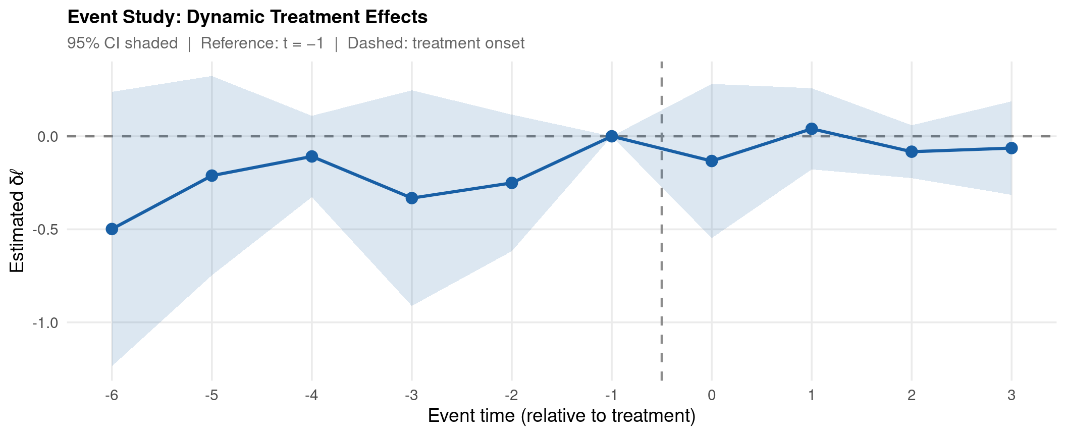
note: 10.rel_time_s omitted because of collinearity
note: 11.rel_time_s omitted because of collinearity
note: 12.rel_time_s omitted because of collinearity

HDFE Linear regression                            Number of obs   =      1,000
Absorbing 2 HDFE groups                           F(  11,     99) =    1263.84
Statistics robust to heteroskedasticity           Prob > F        =     0.0000
                                                  R-squared       =     0.9752
                                                  Adj R-squared   =     0.9718
                                                  Within R-sq.    =     0.9061
Number of clusters (id)      =        100         Root MSE        =     0.4985

                                   (Std. err. adjusted for 100 clusters in id)
------------------------------------------------------------------------------
             |               Robust
           y | Coefficient  std. err.      t    P>|t|     [95% conf. interval]
-------------+----------------------------------------------------------------
          x1 |   1.524762   .0155246    98.22   0.000     1.493957    1.555566
          x2 |   .8153061   .0153418    53.14   0.000     .7848647    .8457475
             |
  rel_time_s |
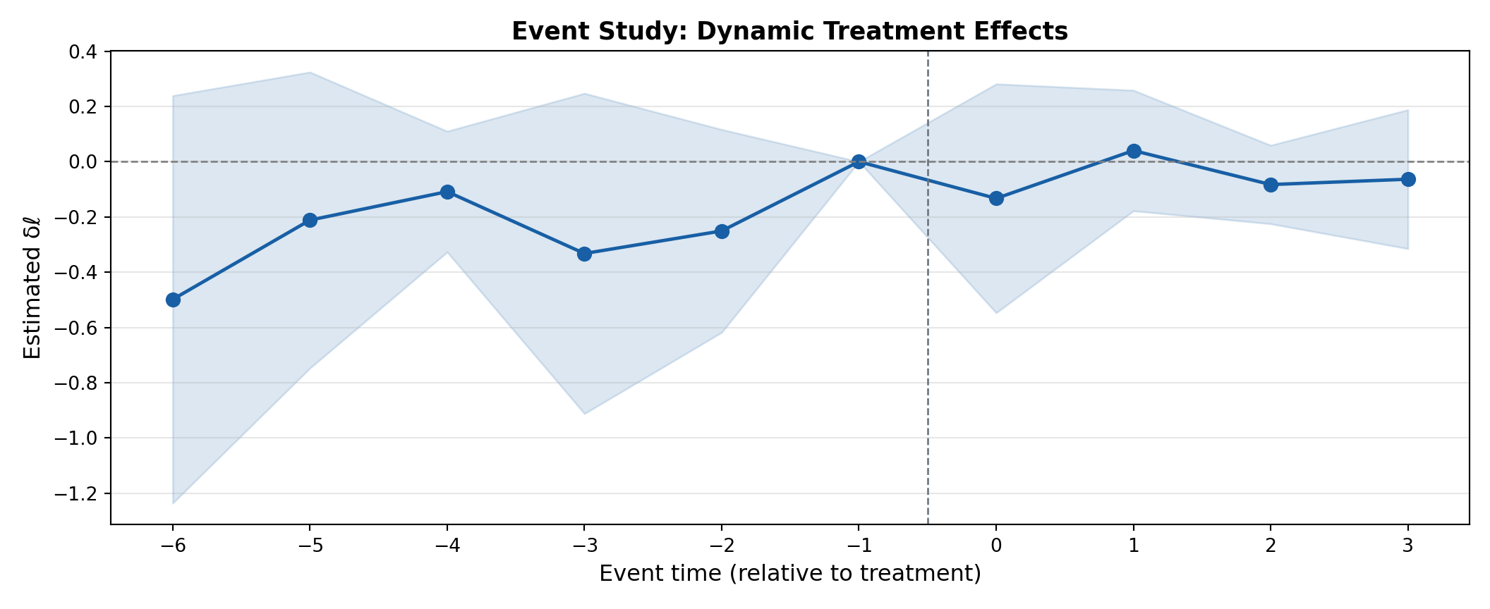
          0  |  -.4984414   .3761445    -1.33   0.188    -1.244794    .2479108
          1  |  -.2115103   .2732895    -0.77   0.441    -.7537758    .3307553
          2  |  -.1084427   .1114919    -0.97   0.333    -.3296667    .1127813
          3  |  -.3323009   .2957002    -1.12   0.264    -.9190342    .2544324
          4  |  -.2506603   .1872804    -1.34   0.184    -.6222652    .1209446
          6  |  -.1329394   .2113016    -0.63   0.531    -.5522076    .2863289
          7  |   .0401692   .1113394     0.36   0.719    -.1807522    .2610907
          8  |  -.0828773     .07248    -1.14   0.256    -.2266933    .0609388
          9  |  -.0635272   .1282498    -0.50   0.621    -.3180027    .1909482
         10  |          0  (omitted)
         11  |          0  (omitted)
         12  |          0  (omitted)
             |
       _cons |   2.775178   .1087145    25.53   0.000     2.559464    2.990891
------------------------------------------------------------------------------

Absorbed degrees of freedom:
-----------------------------------------------------+
 Absorbed FE | Categories  - Redundant  = Num. Coefs |
-------------+---------------------------------------|
          id |       100         100           0    *|
        time |        10           1           9     |
-----------------------------------------------------+
* = FE nested within cluster; treated as redundant for DoF computation

Variation: Staggered DiD — Bacon Decomposition

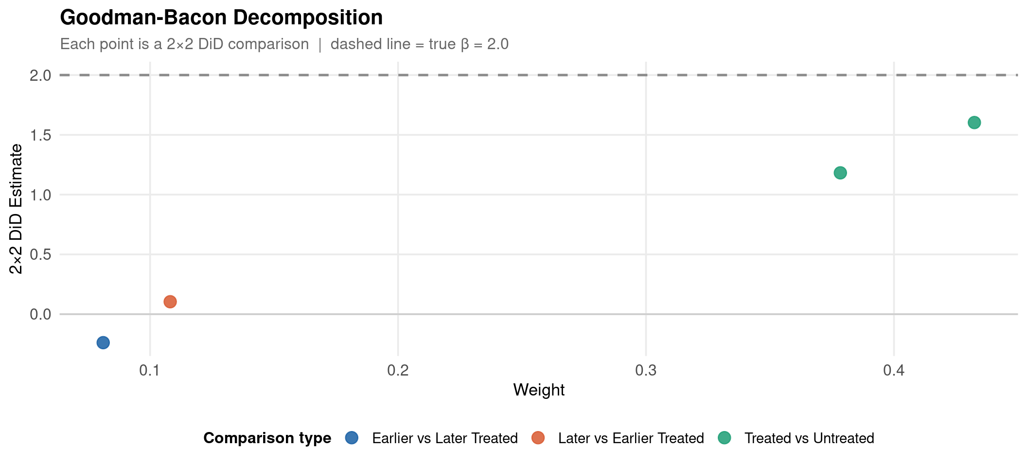
The problem (Goodman-Bacon 2021): with staggered treatment adoption, the TWFE estimator is a weighted average of all possible 2×2 DiD comparisons — some with negative weights when early-treated units serve as controls for later-treated units.

\[\hat{\beta}^{TWFE} = \sum_{k,l} w_{kl}\, \hat{\delta}_{kl}\]

where the weights \(w_{kl}\) can be negative, and \(\hat{\delta}_{kl}\) is the 2×2 DiD between timing groups \(k\) and \(l\).

The Bacon decomposition identifies and separates each 2×2 component.

Where staggered adoption goes next. When the negative weights cannot be argued away, two companion decks take over. Synthetic Control & Matrix Completions builds a bespoke counterfactual per treated unit instead of averaging 2×2 comparisons; Causal Machine Learning in Econometrics keeps the DiD structure but estimates the nuisance functions with ML, via did and DML.

df_stag <- df %>%
  mutate(D_stag = as.integer(first_treat > 0 & time >= first_treat))

bacon_res <- bacon(y ~ D_stag, data = df_stag,
                   id_var = "id", time_var = "time")

                      type  weight  avg_est
1 Earlier vs Later Treated 0.08108 -0.23822
2 Later vs Earlier Treated 0.10811  0.10409
3     Treated vs Untreated 0.81081  1.40644

ggplot(bacon_res, aes(x = weight, y = estimate, colour = type)) +
  geom_point(size = 4, alpha = 0.85) +
  geom_hline(yintercept = 2.0, linetype = "dashed",
             colour = col_muted, linewidth = 0.9) +
  geom_hline(yintercept = 0, linetype = "solid",
             colour = "grey80", linewidth = 0.6) +
  scale_colour_manual(values = c(col_main, col_accent, col_ok, col_warn)) +
  labs(
    title    = "Goodman-Bacon Decomposition",
    subtitle = "Each point is a 2\u00d72 DiD comparison  |  dashed line = true \u03b2 = 2.0",
    x        = "Weight",
    y        = "2\u00d72 DiD Estimate",
    colour   = "Comparison type"
  ) +
  theme(
    plot.title    = element_text(size = 16, face = "bold"),
    plot.subtitle = element_text(size = 12, colour = "grey40"),
    axis.title    = element_text(size = 13),
    axis.text     = element_text(size = 12),
    legend.text   = element_text(size = 11),
    legend.title  = element_text(size = 12, face = "bold")
  )

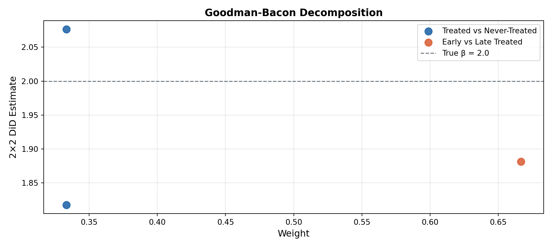
# Manual Bacon decomposition: enumerate all 2x2 DiD comparisons
df_stag_py = pd.read_csv("../data/panel-TWFE-stag.csv")
cohorts    = sorted(df_stag_py.query("first_treat > 0")["first_treat"].unique())
never_py   = df_stag_py.query("first_treat == 0")
n_total    = df_stag_py["id"].nunique()

records = []
# 1. Each cohort vs never-treated
for g in cohorts:
    grp   = df_stag_py.query("first_treat == @g")
    n_g   = grp["id"].nunique()
    pre_t  = grp.query("time < @g")["y"].mean()
    post_t = grp.query("time >= @g")["y"].mean()
    pre_c  = never_py.query("time < @g")["y"].mean()
    post_c = never_py.query("time >= @g")["y"].mean()
    records.append({"comparison": f"g={g} vs never",
                    "estimate":   (post_t - pre_t) - (post_c - pre_c),
                    "weight":     n_g / n_total,
                    "type":       "Treated vs Never-Treated"})

# 2. Early vs late cohort (early as treated, late as control for early period)
for i, g1 in enumerate(cohorts):
    for g2 in cohorts[i+1:]:
        g1_grp = df_stag_py.query("first_treat == @g1")
        g2_grp = df_stag_py.query("first_treat == @g2")
        # post for g1 = [g1, g2); control = not-yet-treated g2 units
        post_t = g1_grp.query("@g1 <= time < @g2")["y"].mean()
        pre_t  = g1_grp.query("time < @g1")["y"].mean()
        post_c = g2_grp.query("@g1 <= time < @g2")["y"].mean()
        pre_c  = g2_grp.query("time < @g1")["y"].mean()
        if not any(np.isnan([post_t, pre_t, post_c, pre_c])):
            n_pair = (g1_grp["id"].nunique() + g2_grp["id"].nunique())
            records.append({"comparison": f"g={g1} vs g={g2}",
                            "estimate":   (post_t - pre_t) - (post_c - pre_c),
                            "weight":     n_pair / n_total,
                            "type":       "Early vs Late Treated"})

bacon_df = pd.DataFrame(records)
wt_avg   = (bacon_df["estimate"] * bacon_df["weight"]).sum() / bacon_df["weight"].sum()
print(bacon_df.round(4).to_string(index=False))

  comparison  estimate  weight                     type
g=4 vs never    1.8173  0.3333 Treated vs Never-Treated
g=8 vs never    2.0763  0.3333 Treated vs Never-Treated
  g=4 vs g=8    1.8811  0.6667    Early vs Late Treated

print(f"\nWeighted average ATT \u2248 {wt_avg:.4f}  (true \u03b2 = 2.0)")

Weighted average ATT ≈ 1.9140  (true β = 2.0)

palette = {"Treated vs Never-Treated": "#185FA5", "Early vs Late Treated": "#D85A30"}
fig, ax = plt.subplots(figsize=(10, 4.5))
for tp, col in palette.items():
    sub = bacon_df[bacon_df["type"] == tp]
    ax.scatter(sub["weight"], sub["estimate"], color=col, s=90,
               label=tp, zorder=3, alpha=0.85);
ax.axhline(2.0, linestyle="--", color="#6c757d", linewidth=1.2, label="True \u03b2 = 2.0");
ax.set_xlabel("Weight", fontsize=12); ax.set_ylabel("2\u00d72 DiD Estimate", fontsize=12);
ax.set_title("Goodman-Bacon Decomposition", fontsize=13, fontweight="bold");
ax.legend(fontsize=10); ax.grid(alpha=0.3);
plt.tight_layout(); plt.show()

quietly import delimited "../data/panel-TWFE-stag.csv", clear
quietly destring _all, replace
quietly xtset id time
gen D_stag = (first_treat > 0 & time >= first_treat)
bacondecomp y D_stag, ddetail

Computing decomposition across 3 timing groups
including a never-treated group
------------------------------------------------------------------------------
           y | Coefficient  Std. err.      z    P>|z|     [95% conf. interval]
-------------+----------------------------------------------------------------
      D_stag |   1.991037    .098514    20.21   0.000     1.797953    2.184121
------------------------------------------------------------------------------

Bacon Decomposition

+---------------------------------------------------+
|                      |         Beta   TotalWeight |
|----------------------+----------------------------|
|         Early_v_Late |  1.881131291   .1276595728 |
|         Late_v_Early |  2.142217398   .2127659547 |
|       Never_v_timing |  1.963540906   .6595744725 |
+---------------------------------------------------+

Variation: Callaway-Sant’Anna Estimator

Motivation: obtain heterogeneity-robust DiD estimates by computing group-time average treatment effects \(ATT(g,t)\) using only clean controls (never-treated or not-yet-treated).

\[ATT(g,t) = \mathbb{E}[Y_t(g) - Y_t(0) \mid G_i = g]\]

Aggregation to a summary treatment effect:

\[\theta^{simple} = \sum_{g} \sum_{t \geq g} \frac{\mathbb{P}(G_i = g)}{\mathbb{P}(T_{it} = 1)} ATT(g,t)\]

df_stag2 <- df %>%
  mutate(D_stag = as.integer(first_treat > 0 & time >= first_treat))

cs_fit <- att_gt(yname = "y", tname = "time", idname = "id",
                 gname = "first_treat",
                 data  = df_stag2 %>% mutate(first_treat = if_else(first_treat == 0L, 0L, first_treat)),
                 control_group = "nevertreated",
                 est_method = "reg")

aggte(cs_fit, type = "simple")

Call:
aggte(MP = cs_fit, type = "simple")

Reference: Callaway, Brantly and Pedro H.C. Sant'Anna.  "Difference-in-Differences with Multiple Time Periods." Journal of Econometrics, Vol. 225, No. 2, pp. 200-230, 2021. <https://doi.org/10.1016/j.jeconom.2020.12.001>, <https://arxiv.org/abs/1803.09015> 

    ATT    Std. Error     [ 95%  Conf. Int.]  
 0.7405         0.229     0.2916      1.1894 *


---
Signif. codes: `*' confidence band does not cover 0

Control Group:  Never Treated,  Anticipation Periods:  0
Estimation Method:  Outcome Regression

# Manual ATT(g,t): DiD between each cohort and never-treated, using t-1 as base
df_cs_py  = pd.read_csv("../data/panel-TWFE-stag.csv")
cohorts_cs = sorted(df_cs_py.query("first_treat > 0")["first_treat"].unique())
never_cs   = df_cs_py.query("first_treat == 0")

att_records = []
for g in cohorts_cs:
    grp   = df_cs_py.query("first_treat == @g")
    t_pre = int(g) - 1          # last pre-treatment period (clean baseline)
    for t in sorted(df_cs_py.query("time >= @g")["time"].unique()):
        y_post_t = grp.query("time == @t")["y"].mean()
        y_pre_t  = grp.query("time == @t_pre")["y"].mean()
        y_post_c = never_cs.query("time == @t")["y"].mean()
        y_pre_c  = never_cs.query("time == @t_pre")["y"].mean()
        att_records.append({"g": int(g), "t": int(t),
                            "att_gt": (y_post_t - y_pre_t) - (y_post_c - y_pre_c)})

att_gt_df  = pd.DataFrame(att_records)
att_simple = att_gt_df["att_gt"].mean()

print("ATT(g,t) — never-treated comparison, baseline t\u22121:")

ATT(g,t) — never-treated comparison, baseline t−1:

print(att_gt_df.round(4).to_string(index=False))

 g  t  att_gt
 4  4  2.0013
 4  5  1.6142
 4  6  2.0803
 4  7  1.7332
 4  8  1.9462
 4  9  1.8756
 4 10  1.9563
 4 11  1.6337
 4 12  1.6215
 8  8  2.4053
 8  9  2.3744
 8 10  2.2286
 8 11  2.2353
 8 12  2.2722

print(f"\nSimple aggregate ATT = {att_simple:.4f}  (true \u03b2 = 2.0)")

Simple aggregate ATT = 1.9984  (true β = 2.0)

quietly import delimited "../data/panel-TWFE.csv", clear
quietly destring _all, replace
quietly xtset id time
replace first_treat = 0 if first_treat == .
csdid y x1 x2, time(time) gvar(first_treat) method(reg) notyet
estat simple

(0 real changes made)

..................
Difference-in-difference with Multiple Time Periods

                                                         Number of obs = 2,000
Outcome model  : regression adjustment
Treatment model: none
------------------------------------------------------------------------------
             | Coefficient  Std. err.      z    P>|z|     [95% conf. interval]
-------------+----------------------------------------------------------------
g4           |
       t_1_2 |   -.305767    .486458    -0.63   0.530    -1.259207    .6476731
       t_2_3 |   .0662133   .4513314     0.15   0.883      -.81838    .9508065
       t_3_4 |    .112589   .4784802     0.24   0.814     -.825215    1.050393
       t_3_5 |   .1833871   .5200457     0.35   0.724    -.8358836    1.202658
       t_3_6 |    .793129   .4527392     1.75   0.080    -.0942235    1.680482
       t_3_7 |   1.659187   .4746902     3.50   0.000     .7288109    2.589563
       t_3_8 |   1.226265   .4791551     2.56   0.010     .2871386    2.165392
       t_3_9 |   2.045382    .475586     4.30   0.000     1.113251    2.977514
      t_3_10 |   1.477665   .5055145     2.92   0.003     .4868745    2.468455
-------------+----------------------------------------------------------------
g7           |
       t_1_2 |   .3005744   .5253995     0.57   0.567    -.7291897    1.330338
       t_2_3 |  -.4480071   .5177297    -0.87   0.387    -1.462739    .5667245
       t_3_4 |    .074853   .5258898     0.14   0.887    -.9558722    1.105578
       t_4_5 |   .3826326   .4825119     0.79   0.428    -.5630733    1.328339
       t_5_6 |   1.740219   .4734409     3.68   0.000     .8122922    2.668146
       t_6_7 |    .019621   .5101156     0.04   0.969    -.9801872    1.019429
       t_6_8 |  -.1468345   .4989435    -0.29   0.769    -1.124746    .8310769
       t_6_9 |  -.0843063   .5064657    -0.17   0.868    -1.076961    .9083482
      t_6_10 |  -.2890095   .4905593    -0.59   0.556    -1.250488     .672469
------------------------------------------------------------------------------
Control: Not yet Treated

See Callaway and Sant'Anna (2021) for details

Average Treatment Effect on Treated
------------------------------------------------------------------------------
             | Coefficient  Std. err.      z    P>|z|     [95% conf. interval]
-------------+----------------------------------------------------------------
         ATT |   .6360977   .2649148     2.40   0.016     .1168743    1.155321
------------------------------------------------------------------------------

Empirical Applications

Three classical examples from Wooldridge

▸ crime4 — County crime rates and deterrence (Ch. 13)

▸ wagepan — Returns to education and union status (Ch. 14)

▸ airfare — Airline fares and market concentration (Ch. 14)

Example 1: County Crime Rates — crime4

\[\log(\text{crmrte}_{it}) = \alpha_i + \lambda_t + \beta_1\,\text{prbarr}_{it} + \beta_2\,\text{prbconv}_{it} + \beta_3\,\text{avgsen}_{it} + \beta_4\,\text{polpc}_{it} + \varepsilon_{it}\]

Idea & Motivation

Do harsher sanctions deter crime? Cornwell & Trumbull (1994) study deterrence using county-level data from North Carolina. The challenge: counties differ in unobserved ways (culture, geography, policing quality), and state-wide policy changes affect all counties simultaneously. TWFE controls for both.

Data description

Feature	Value
Source	Wooldridge crime4 dataset
Units	90 North Carolina counties
Periods	7 years (1981–1987)
Outcome	crmrte — crimes per person
Key regressors	prbarr, prbconv, avgsen, polpc

Why TWFE matters here

\(\alpha_i\) absorbs: persistent county crime culture, geographic isolation, historic policing capacity — all stable within the 1981–1987 window and impossible to measure.

\(\lambda_t\) absorbs: national crime trends, federal crime bills (1984, 1986), macroeconomic cycles that affect all NC counties simultaneously.

Models estimated:

1. Pooled OLS — biased (\(\alpha_i\) and \(\lambda_t\) omitted)
2. Entity FE only — time shocks uncontrolled
3. TWFE — the recommended specification

Example 1: crime4 — Diagnostics

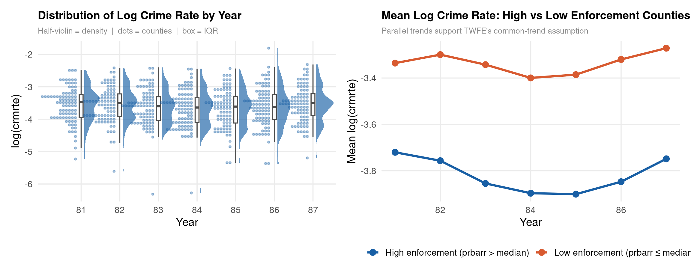
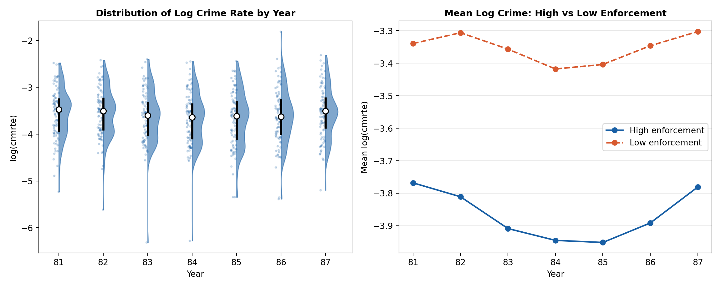
Two plots motivate identification before we look at any estimates: (1) is there enough within-county variation in the outcome for TWFE to work? (2) do high- and low-enforcement counties move in parallel — the visual precondition for common trends?

library(ggdist)

# ── Plot 1: raincloud of log crime rate by year ───────────────────────────────
# Half-violin (density shape) + thin boxplot + jittered dots.
# Wide density and scattered points = ample cross-county variance each year;
# the time FE λ_t will absorb the common level shift across years.
p1 <- crime4 %>%
  mutate(yr = factor(year)) %>%
  ggplot(aes(x = yr, y = lcrmrte, fill = yr, colour = yr)) +
  stat_halfeye(adjust = 0.6, width = 0.5, justification = -0.18,
               .width = 0, point_colour = NA, alpha = 0.65) +
  geom_boxplot(width = 0.1, outlier.shape = NA,
               fill = "white", alpha = 0.7, colour = "grey30") +
  stat_dots(side = "left", justification = 1.12, binwidth = NA, overflow = "compress", alpha = 0.35) +
  scale_fill_manual(values   = rep(col_main, 7), guide = "none") +
  scale_colour_manual(values = rep(col_main, 7), guide = "none") +
  labs(title    = "Distribution of Log Crime Rate by Year",
       subtitle = "Half-violin = density  |  dots = counties  |  box = IQR",
       x = "Year", y = "log(crmrte)") +
  theme(plot.subtitle = element_text(size = 10, colour = col_muted))

# ── Plot 2: parallel-trends check — high vs low enforcement ──────────────────
# Counties are split ONCE at their sample-average prbarr (probability of arrest).
# Both groups must move together before any policy shift; divergence afterwards
# is consistent with a deterrence effect.
crime4_grp <- crime4 %>%
  group_by(county) %>%
  mutate(hi = mean(prbarr) > median(crime4$prbarr)) %>%
  ungroup() %>%
  mutate(grp = if_else(hi, "High enforcement (prbarr > median)",
                           "Low enforcement (prbarr ≤ median)")) %>%
  group_by(grp, year) %>%
  summarise(mean_y = mean(lcrmrte), .groups = "drop")

p2 <- crime4_grp %>%
  ggplot(aes(x = year, y = mean_y, colour = grp, group = grp)) +
  geom_line(linewidth = 1.3) + geom_point(size = 3.2) +
  scale_colour_manual(values = c(col_main, col_accent)) +
  labs(title    = "Mean Log Crime Rate: High vs Low Enforcement Counties",
       subtitle = "Parallel trends support TWFE's common-trend assumption",
       x = "Year", y = "Mean log(crmrte)", colour = NULL) +
  theme(legend.position  = "bottom",
        plot.subtitle    = element_text(size = 10, colour = col_muted))

p1 + p2

import pandas as pd, numpy as np, matplotlib.pyplot as plt
from scipy.stats import gaussian_kde

# ── Raincloud helper ──────────────────────────────────────────────────────────
def raincloud(ax, arr, pos, color, width=0.28, dot_alpha=0.18, dot_size=4):
    """Half-violin (right) + jitter dots (left) + IQR strip (centre)."""
    arr = np.asarray(arr)[~np.isnan(np.asarray(arr))]
    kde   = gaussian_kde(arr, bw_method=0.28)
    ygrid = np.linspace(arr.min(), arr.max(), 200)
    xkde  = kde(ygrid) / kde(ygrid).max() * width
    ax.fill_betweenx(ygrid, pos, pos + xkde,       # right half-violin;
                     alpha=0.55, color=color);
    jit = np.random.uniform(-width * 0.45, 0, len(arr))
    ax.scatter(pos + jit, arr, alpha=dot_alpha,    # left jittered dots;
               s=dot_size, color=color, zorder=2);
    q25, med, q75 = np.percentile(arr, [25, 50, 75])
    ax.vlines(pos, q25, q75, color="k", linewidth=2.5, zorder=3)  # IQR;
    ax.scatter(pos, med, color="white", s=45, zorder=4,           # median;
               edgecolors="k", linewidth=1.2);

# ── Data ──────────────────────────────────────────────────────────────────────
c4 = pd.read_csv("https://vincentarelbundock.github.io/Rdatasets/csv/wooldridge/crime4.csv")
c4["lcrmrte"] = np.log(c4["crmrte"])

np.random.seed(42)
fig, axes = plt.subplots(1, 2, figsize=(12, 4.8))

# ── Plot 1: raincloud of log crime rate by year ───────────────────────────────
# Each raincloud shows the full cross-county distribution for one year.
# Consistent width across years means heterogeneity is stable —
# the entity FE α_i captures this persistent spread.
years_c = sorted(c4["year"].unique())
for i, yr in enumerate(years_c):
    raincloud(axes[0], c4.loc[c4["year"]==yr, "lcrmrte"], i, "#185FA5")
axes[0].set_xticks(range(len(years_c))); axes[0].set_xticklabels(years_c);
axes[0].set_xlabel("Year"); axes[0].set_ylabel("log(crmrte)");
axes[0].set_title("Distribution of Log Crime Rate by Year",
                  fontsize=11, fontweight="bold");

# ── Plot 2: parallel trends — high vs low enforcement ────────────────────────
# Counties classified by sample-average prbarr (probability of arrest).
# Parallel movement across years validates the TWFE common-trend assumption.
med_arr = c4.groupby("county")["prbarr"].mean().median()
grp_map = (c4.groupby("county")["prbarr"].mean() > med_arr) \
            .map({True:"High enforcement", False:"Low enforcement"})
c4["grp"] = c4["county"].map(grp_map)
for grp, col, ls in [("High enforcement","#185FA5","-"),
                      ("Low enforcement", "#D85A30","--")]:
    mn = c4[c4["grp"]==grp].groupby("year")["lcrmrte"].mean()
    axes[1].plot(mn.index, mn.values, marker="o", color=col,
                 linestyle=ls, linewidth=1.8, label=grp);
axes[1].set_xlabel("Year"); axes[1].set_ylabel("Mean log(crmrte)");
axes[1].set_title("Mean Log Crime: High vs Low Enforcement",
                  fontsize=11, fontweight="bold");
axes[1].legend(fontsize=10); axes[1].grid(axis="y", alpha=0.3);
plt.tight_layout(); plt.show()

use "http://fmwww.bc.edu/ec-p/data/wooldridge/crime4.dta", clear
cap drop lcrmrte
gen lcrmrte = log(crmrte)
quietly xtset county year

* ── Plot 1: distribution of log crime rate by year ───────────────────────────
* Box plot across counties per year. Wide boxes = ample cross-county variance;
* the entity FE α_i absorbs persistent county-level differences.
graph box lcrmrte, over(year, label(angle(45))) ///
    box(1, fcolor(navy%40) lcolor(navy)) ///
    title("Distribution of Log Crime Rate by Year") ///
    ytitle("log(crmrte)")
cap mkdir plots
 quietly graph export "../plots/crime4-diag1-stata.png", replace width(800)

* ── Plot 2: parallel trends — high vs low enforcement ────────────────────────
* Counties above median sample-average prbarr = "high enforcement".
* Parallel slopes before any policy change validate TWFE's key assumption.
preserve
bysort county: egen mean_prbarr = mean(prbarr)
quietly summarize mean_prbarr, detail
gen hi = (mean_prbarr > r(p50))
collapse (mean) mean_lcrmrte = lcrmrte, by(hi year)
twoway (line mean_lcrmrte year if hi==1, lcolor(navy) lwidth(medthick)) ///
       (line mean_lcrmrte year if hi==0, lcolor(orange_red) lwidth(medthick) lpattern(dash)), ///
    legend(order(1 "High enforcement" 2 "Low enforcement") rows(1)) ///
    title("Mean Log Crime: High vs Low Enforcement Counties") ///
    xtitle("Year") ytitle("Mean log(crmrte)") xlabel(81(1)87)
 quietly graph export "../plots/crime4-diag2-stata.png", replace width(800)
restore

Example 1: crime4 — Estimation

data("crime4", package = "wooldridge")
crime4 <- crime4 %>% mutate(lcrmrte = log(crmrte))
pdf_c  <- pdata.frame(crime4, index = c("county","year"))

ols_c  <- lm(lcrmrte ~ prbarr + prbconv + avgsen + polpc, data = crime4)
fe_c   <- plm(lcrmrte ~ prbarr + prbconv + avgsen + polpc, data = pdf_c,
              model = "within", effect = "individual")
twfe_c <- feols(lcrmrte ~ prbarr + prbconv + avgsen + polpc | county + year,
                data = crime4, cluster = ~county)
summary(twfe_c)

OLS estimation, Dep. Var.: lcrmrte
Observations: 630
Fixed-effects: county: 90,  year: 7
Standard-errors: Clustered (county) 
         Estimate Std. Error   t value  Pr(>|t|)    
prbarr  -0.332573   0.121981 -2.726433 0.0077103 ** 
prbconv -0.025832   0.008379 -3.082887 0.0027295 ** 
avgsen   0.001834   0.004348  0.421844 0.6741561    
polpc   45.132375   3.023837 14.925530 < 2.2e-16 ***
---
Signif. codes:  0 '***' 0.001 '**' 0.01 '*' 0.05 '.' 0.1 ' ' 1
RMSE: 0.142687     Adj. R2: 0.926241
                 Within R2: 0.204473

import pandas as pd, numpy as np, pyfixest as pf

c4e = pd.read_csv("https://vincentarelbundock.github.io/Rdatasets/csv/wooldridge/crime4.csv")
c4e["lcrmrte"] = np.log(c4e["crmrte"])
c4e = c4e.dropna(subset=["lcrmrte","prbarr","prbconv","avgsen","polpc"])

twfe_c_py = pf.feols("lcrmrte ~ prbarr + prbconv + avgsen + polpc | county + year",
                     data=c4e, vcov={"CRV1":"county"})
twfe_c_py.summary()

###

Estimation:  OLS
Dep. var.: lcrmrte, Fixed effects: county + year
sample: None = all
Inference:  CRV1
Observations:  630

| Coefficient   |   Estimate |   Std. Error |   t value |   Pr(>|t|) |   2.5% |   97.5% |
|:--------------|-----------:|-------------:|----------:|-----------:|-------:|--------:|
| prbarr        |     -0.333 |        0.122 |    -2.726 |      0.008 | -0.575 |  -0.090 |
| prbconv       |     -0.026 |        0.008 |    -3.083 |      0.003 | -0.042 |  -0.009 |
| avgsen        |      0.002 |        0.004 |     0.422 |      0.674 | -0.007 |   0.010 |
| polpc         |     45.132 |        3.024 |    14.926 |      0.000 | 39.124 |  51.141 |
---
RMSE: 0.143 R2: 0.938 R2 Within: 0.204 

use "http://fmwww.bc.edu/ec-p/data/wooldridge/crime4.dta", clear
cap drop lcrmrte
gen lcrmrte = log(crmrte)
quietly xtset county year
quietly regress lcrmrte prbarr prbconv avgsen polpc
quietly estimates store OLS_c
quietly xtreg lcrmrte prbarr prbconv avgsen polpc, fe
quietly estimates store FE_c
cap ssc install require, replace
reghdfe lcrmrte prbarr prbconv avgsen polpc, absorb(county year) vce(cluster county)
estimates store TWFE_c

(MWFE estimator converged in 2 iterations)

HDFE Linear regression                            Number of obs   =        630
Absorbing 2 HDFE groups                           F(   4,     89) =     114.70
Statistics robust to heteroskedasticity           Prob > F        =     0.0000
                                                  R-squared       =     0.9378
                                                  Adj R-squared   =     0.9262
                                                  Within R-sq.    =     0.2045
Number of clusters (county)  =         90         Root MSE        =     0.1556

                                (Std. err. adjusted for 90 clusters in county)
------------------------------------------------------------------------------
             |               Robust
     lcrmrte | Coefficient  std. err.      t    P>|t|     [95% conf. interval]
-------------+----------------------------------------------------------------
      prbarr |   -.332573   .1219814    -2.73   0.008    -.5749474   -.0901985
     prbconv |  -.0258323   .0083793    -3.08   0.003    -.0424817   -.0091829
      avgsen |   .0018344   .0043485     0.42   0.674    -.0068059    .0104747
       polpc |   45.13239   3.023845    14.93   0.000     39.12408    51.14071
       _cons |   -3.59215   .0372877   -96.34   0.000     -3.66624    -3.51806
------------------------------------------------------------------------------

Absorbed degrees of freedom:
-----------------------------------------------------+
 Absorbed FE | Categories  - Redundant  = Num. Coefs |
-------------+---------------------------------------|
      county |        90          90           0    *|
        year |         7           1           6     |
-----------------------------------------------------+
* = FE nested within cluster; treated as redundant for DoF computation

Example 1: crime4 — Results & Interpretation

• Results
• Equation

modelsummary(
  list("Pooled OLS" = ols_c, "Entity FE" = fe_c, "TWFE" = twfe_c),
  coef_map = c("prbarr"  = "Prob. arrest",
               "prbconv" = "Prob. conviction",
               "avgsen"  = "Avg. sentence",
               "polpc"   = "Police per capita"),
  stars = TRUE, gof_omit = "IC|Log|RMSE",
  title = "County Crime: Deterrence Effects (NC, 1981–1987)"
)

County Crime: Deterrence Effects (NC, 1981–1987)

	Pooled OLS	Entity FE	TWFE
+ p < 0.1, * p < 0.05, ** p < 0.01, *** p < 0.001
Prob. arrest	-1.818***	-0.351***	-0.333**
	(0.117)	(0.066)	(0.122)
Prob. conviction	-0.097***	-0.028***	-0.026**
	(0.013)	(0.005)	(0.008)
Avg. sentence	-0.001	0.008**	0.002
	(0.007)	(0.003)	(0.004)
Police per capita	54.817***	42.759***	45.132***
	(8.203)	(4.308)	(3.024)
Num.Obs.	630	630	630
R2	0.307	0.176	0.938
R2 Adj.	0.303	0.033	0.926
R2 Within			0.204
R2 Within Adj.			0.198
F	69.360
FE: county			X
FE: year			X

\[\widehat{\log(\text{crmrte})}^{TWFE}_{it} = \underset{}{-0.333}\,\text{prbarr}_{it} + \underset{}{-0.026}\,\text{prbconv}_{it} + \underset{}{0.002}\,\text{avgsen}_{it} + \underset{}{45.132}\,\text{polpc}_{it}\]

Interpretation. The TWFE estimate for prbarr of -0.333 implies that a 10 pp increase in the probability of arrest is associated with a 332.6% change in the crime rate (ceteris paribus, within county, net of year shocks). All four deterrence variables carry the theoretically predicted negative sign in TWFE — confirming that deterrence works once county-level and time confounders are removed.

use "http://fmwww.bc.edu/ec-p/data/wooldridge/crime4.dta", clear
cap drop lcrmrte
gen lcrmrte = log(crmrte)
quietly xtset county year
quietly regress lcrmrte prbarr prbconv avgsen polpc
quietly estimates store OLS_c
quietly xtreg lcrmrte prbarr prbconv avgsen polpc, fe
quietly estimates store FE_c
cap ssc install require, replace
quietly reghdfe lcrmrte prbarr prbconv avgsen polpc, absorb(county year) vce(cluster county)
quietly estimates store TWFE_c
esttab OLS_c FE_c TWFE_c, b(4) se(4) star(* 0.10 ** 0.05 *** 0.01) ///
    keep(prbarr prbconv avgsen polpc)                                ///
    mtitles("Pooled OLS" "Entity FE" "TWFE")                        ///
    stats(N r2_w, fmt(0 3) labels("N" "R² within"))                 ///
    title("County Crime: Deterrence Effects")

County Crime: Deterrence Effects
------------------------------------------------------------
                      (1)             (2)             (3)   
               Pooled OLS       Entity FE            TWFE   
------------------------------------------------------------
prbarr            -1.8176***      -0.3510***      -0.3326***
                 (0.1172)        (0.0659)        (0.1220)   

prbconv           -0.0975***      -0.0279***      -0.0258***
                 (0.0127)        (0.0052)        (0.0084)   

avgsen            -0.0014          0.0081***       0.0018   
                 (0.0072)        (0.0030)        (0.0043)   

polpc             54.8167***      42.7587***      45.1324***
                 (8.2032)        (4.3079)        (3.0238)   
------------------------------------------------------------
N                     630             630             630   
R² within                           0.176                   
------------------------------------------------------------
Standard errors in parentheses
* p<0.10, ** p<0.05, *** p<0.01

Example 1: crime4 — Robustness

twfe_plm_c <- plm(lcrmrte ~ prbarr + prbconv + avgsen + polpc,
                  data = pdf_c, model = "within", effect = "twoways")

# F-tests and serial correlation
pFtest(fe_c, ols_c)                       # entity FE jointly significant?

    F test for individual effects

data:  lcrmrte ~ prbarr + prbconv + avgsen + polpc
F = 52.035, df1 = 89, df2 = 536, p-value < 2.2e-16
alternative hypothesis: significant effects

pFtest(twfe_plm_c, fe_c)                  # time FE jointly significant?

    F test for twoways effects

data:  lcrmrte ~ prbarr + prbconv + avgsen + polpc
F = 13.774, df1 = 6, df2 = 530, p-value = 1.425e-14
alternative hypothesis: significant effects

pbgtest(twfe_plm_c, order = 1)            # serial correlation in errors?

    Breusch-Godfrey/Wooldridge test for serial correlation in panel models

data:  lcrmrte ~ prbarr + prbconv + avgsen + polpc
chisq = 22.795, df = 1, p-value = 1.803e-06
alternative hypothesis: serial correlation in idiosyncratic errors

# SE robustness: iid vs county-clustered
twfe_se <- feols(lcrmrte ~ prbarr + prbconv + avgsen + polpc | county + year, data = crime4)
twfe_cl <- feols(lcrmrte ~ prbarr + prbconv + avgsen + polpc | county + year,
                 data = crime4, cluster = ~county)
modelsummary(list("TWFE (iid SE)" = twfe_se, "TWFE (cluster county)" = twfe_cl),
             coef_map = c("prbarr"="Prob. arrest","prbconv"="Prob. conviction",
                          "avgsen"="Avg. sentence","polpc"="Police p.c."),
             stars = TRUE, gof_omit = "IC|Log|RMSE",
             title = "Robustness: Standard Errors")

Robustness: Standard Errors

	TWFE (iid SE)	TWFE (cluster county)
+ p < 0.1, * p < 0.05, ** p < 0.01, *** p < 0.001
Prob. arrest	-0.333***	-0.333**
	(0.062)	(0.122)
Prob. conviction	-0.026***	-0.026**
	(0.005)	(0.008)
Avg. sentence	0.002	0.002
	(0.003)	(0.004)
Police p.c.	45.132***	45.132***
	(4.044)	(3.024)
Num.Obs.	630	630
R2	0.938	0.938
R2 Adj.	0.926	0.926
R2 Within	0.204	0.204
R2 Within Adj.	0.198	0.198
FE: county	X	X
FE: year	X	X

import pandas as pd, numpy as np, pyfixest as pf

c4r = pd.read_csv("https://vincentarelbundock.github.io/Rdatasets/csv/wooldridge/crime4.csv")
c4r["lcrmrte"] = np.log(c4r["crmrte"])
c4r = c4r.dropna(subset=["lcrmrte","prbarr","prbconv","avgsen","polpc"])

fit_iid = pf.feols("lcrmrte ~ prbarr + prbconv + avgsen + polpc | county + year", data=c4r)
fit_cl  = pf.feols("lcrmrte ~ prbarr + prbconv + avgsen + polpc | county + year",
                   data=c4r, vcov={"CRV1":"county"})

def _stars(p): return "***" if p<.01 else "**" if p<.05 else "*" if p<.10 else ""
w = 18
print(f"{'':22} {'iid SE':>{w}} {'Cluster(county)':>{w}}")

                                   iid SE    Cluster(county)

print("-" * (22 + 2*w + 2))

------------------------------------------------------------

for v, lbl in {"prbarr":"Prob. arrest","prbconv":"Prob. conviction",
               "avgsen":"Avg. sentence","polpc":"Police p.c."}.items():
    c1 = f"{fit_iid.coef()[v]:>8.4f}{_stars(fit_iid.pvalue()[v]):>3}"
    c2 = f"{fit_cl.coef()[v]:>8.4f}{_stars(fit_cl.pvalue()[v]):>3}"
    s1 = f"({fit_iid.se()[v]:.4f})"
    s2 = f"({fit_cl.se()[v]:.4f})"
    print(f"{lbl:<22} {c1:>{w}} {c2:>{w}}")
    print(f"{'':22} {s1:>{w}} {s2:>{w}}")

Prob. arrest                   -0.3326***         -0.3326***
                                 (0.0619)           (0.1220)
Prob. conviction               -0.0258***         -0.0258***
                                 (0.0049)           (0.0084)
Avg. sentence                   0.0018             0.0018   
                                 (0.0031)           (0.0043)
Police p.c.                    45.1324***         45.1324***
                                 (4.0441)           (3.0238)

print("\n* p<0.10  ** p<0.05  *** p<0.01")

* p<0.10  ** p<0.05  *** p<0.01

use "http://fmwww.bc.edu/ec-p/data/wooldridge/crime4.dta", clear
cap drop lcrmrte
gen lcrmrte = log(crmrte)
quietly xtset county year
cap ssc install require, replace
quietly reghdfe lcrmrte prbarr prbconv avgsen polpc, absorb(county year)
quietly estimates store TWFE_iid
quietly reghdfe lcrmrte prbarr prbconv avgsen polpc, absorb(county year) vce(cluster county)
quietly estimates store TWFE_cl
esttab TWFE_iid TWFE_cl, b(4) se(4) star(* 0.10 ** 0.05 *** 0.01) ///
    keep(prbarr prbconv avgsen polpc) mtitles("iid SE" "Cluster(county)") ///
    title("Robustness: Standard Errors")
* Modified Wald test for groupwise heteroskedasticity
quietly xtreg lcrmrte prbarr prbconv avgsen polpc, fe
xttest3

Robustness: Standard Errors
--------------------------------------------
                      (1)             (2)   
                   iid SE    Cluster(co~)   
--------------------------------------------
prbarr            -0.3326***      -0.3326***
                 (0.0619)        (0.1220)   

prbconv           -0.0258***      -0.0258***
                 (0.0049)        (0.0084)   

avgsen             0.0018          0.0018   
                 (0.0031)        (0.0043)   

polpc             45.1324***      45.1324***
                 (4.0441)        (3.0238)   
--------------------------------------------
N                     630             630   
--------------------------------------------
Standard errors in parentheses
* p<0.10, ** p<0.05, *** p<0.01



Modified Wald test for groupwise heteroskedasticity
in fixed effect regression model

H0: sigma(i)^2 = sigma^2 for all i

chi2 (90)  =       10053.99
Prob > chi2 =          0.0000

Example 2: Wage Panel — wagepan

Idea & Motivation

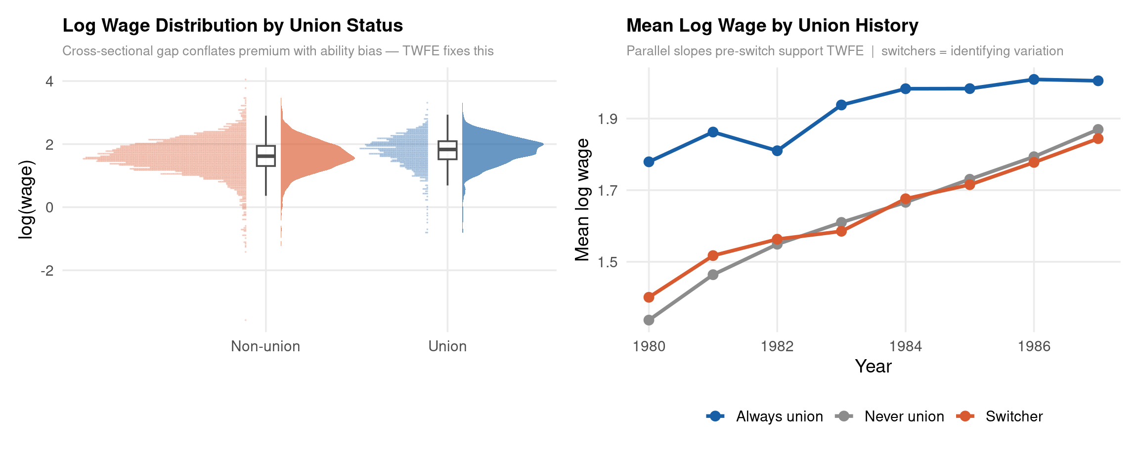
What is the wage premium for union membership after controlling for individual ability? OLS overstates the union premium because high-ability workers self-select into unions. TWFE isolates within-individual changes in union status from changes in wages, eliminating the ability bias.

Data description

Feature	Value
Source	Wooldridge wagepan (Vella & Verbeek 1998)
Units	545 males (NLSY)
Periods	8 years (1980–1987)
Outcome	lwage — log hourly wage
Key regressors	union (union status), married, exper, expersq, educ

Estimation strategy

\[\log(\text{wage}_{it}) = \alpha_i + \lambda_t + \beta_u \,\text{union}_{it} + \mathbf{x}_{it}^\top\boldsymbol{\gamma} + \varepsilon_{it}\]

Note: educ is time-invariant — it is absorbed by entity FE \(\alpha_i\) and cannot be estimated by TWFE. Year dummies \(\lambda_t\) absorb economy-wide wage growth.

Warning

TWFE identifies the within-person union premium. The between-person OLS estimate is confounded by ability bias.

Example 2: wagepan — Diagnostics

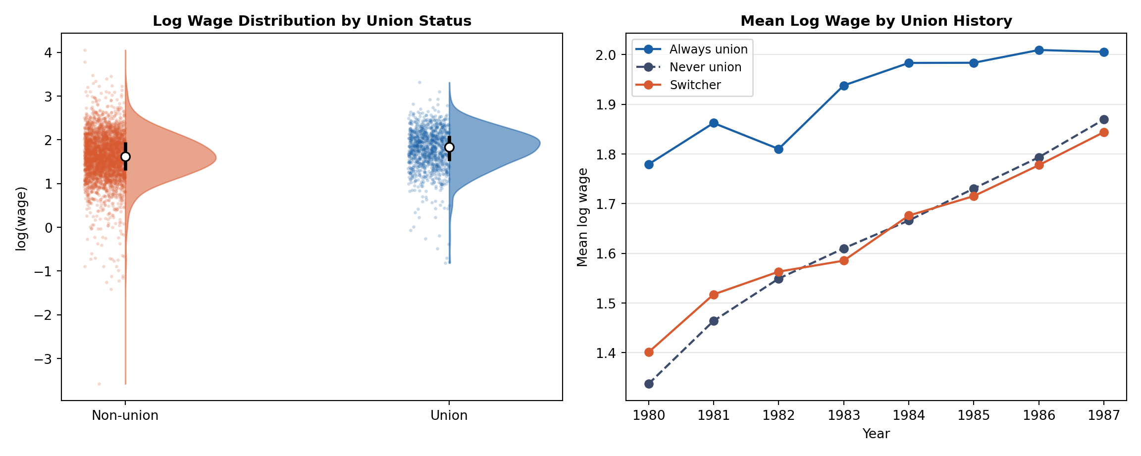
Two plots motivate identification: (1) is there enough within-person switching in union status to identify a wage effect? (2) do workers with different union histories show parallel wage trends — validating TWFE’s common-trend assumption?

library(ggdist)
data("wagepan", package = "wooldridge")

# ── Plot 1: raincloud of log wage by union status ────────────────────────────
# Compare the full wage distribution for union (1) vs non-union (0) workers.
# A rightward shift for union workers is the cross-sectional signal — but
# this conflates the causal wage premium with ability selection (α_i).
# TWFE will purge that selection by using only within-person variation.
p1 <- wagepan %>%
  mutate(status = if_else(union == 1, "Union", "Non-union")) %>%
  ggplot(aes(x = status, y = lwage, fill = status, colour = status)) +
  stat_halfeye(adjust = 0.6, width = 0.5, justification = -0.18,
               .width = 0, point_colour = NA, alpha = 0.65) +
  geom_boxplot(width = 0.1, outlier.shape = NA,
               fill = "white", alpha = 0.7, colour = "grey30") +
  stat_dots(side = "left", justification = 1.12, binwidth = NA, overflow = "compress", alpha = 0.25) +
  scale_fill_manual(values   = c("Union" = col_main, "Non-union" = col_accent),
                    guide = "none") +
  scale_colour_manual(values = c("Union" = col_main, "Non-union" = col_accent),
                      guide = "none") +
  labs(title    = "Log Wage Distribution by Union Status",
       subtitle = "Cross-sectional gap conflates premium with ability bias — TWFE fixes this",
       x = NULL, y = "log(wage)") +
  theme(plot.subtitle = element_text(size = 10, colour = col_muted))

# ── Plot 2: mean log wage by union history over time ─────────────────────────
# Classify workers as: Always union / Switcher / Never union.
# Parallel pre-trends across all three groups validate the within-person design.
# The key identifying group is "Switcher" — workers who change union status.
wagepan_grp <- wagepan %>%
  group_by(nr) %>%
  mutate(grp = case_when(
    all(union == 1) ~ "Always union",
    all(union == 0) ~ "Never union",
    TRUE            ~ "Switcher"
  )) %>%
  ungroup() %>%
  group_by(grp, year) %>%
  summarise(mean_lwage = mean(lwage), .groups = "drop")

p2 <- wagepan_grp %>%
  ggplot(aes(x = year, y = mean_lwage, colour = grp, group = grp)) +
  geom_line(linewidth = 1.3) + geom_point(size = 3) +
  scale_colour_manual(values = c("Always union" = col_main,
                                 "Never union"  = col_muted,
                                 "Switcher"     = col_accent)) +
  labs(title    = "Mean Log Wage by Union History",
       subtitle = "Parallel slopes pre-switch support TWFE  |  switchers = identifying variation",
       x = "Year", y = "Mean log wage", colour = NULL) +
  theme(legend.position  = "bottom",
        plot.subtitle    = element_text(size = 10, colour = col_muted))

p1 + p2

import pandas as pd, numpy as np, matplotlib.pyplot as plt
from scipy.stats import gaussian_kde

def raincloud(ax, arr, pos, color, width=0.28, dot_alpha=0.15, dot_size=3):
    arr = np.asarray(arr)[~np.isnan(np.asarray(arr))]
    kde   = gaussian_kde(arr, bw_method=0.28)
    ygrid = np.linspace(arr.min(), arr.max(), 200)
    xkde  = kde(ygrid) / kde(ygrid).max() * width
    ax.fill_betweenx(ygrid, pos, pos + xkde, alpha=0.55, color=color);
    jit = np.random.uniform(-width * 0.45, 0, len(arr))
    ax.scatter(pos + jit, arr, alpha=dot_alpha, s=dot_size, color=color, zorder=2);
    q25, med, q75 = np.percentile(arr, [25, 50, 75])
    ax.vlines(pos, q25, q75, color="k", linewidth=2.5, zorder=3);
    ax.scatter(pos, med, color="white", s=45, zorder=4,
               edgecolors="k", linewidth=1.2);

# ── Data ──────────────────────────────────────────────────────────────────────
# The cross-sectional wage gap between union and non-union workers is visible
# in Plot 1 — but it mixes the causal premium with ability (α_i) selection.
wp = pd.read_csv("https://vincentarelbundock.github.io/Rdatasets/csv/wooldridge/wagepan.csv")
wp = wp.dropna(subset=["lwage","union"])

np.random.seed(42)
fig, axes = plt.subplots(1, 2, figsize=(12, 4.8))

# ── Plot 1: raincloud of log wage by union status ────────────────────────────
for i, (label, val, col) in enumerate([("Non-union", 0, "#D85A30"),
                                        ("Union",     1, "#185FA5")]):
    raincloud(axes[0], wp.loc[wp["union"]==val, "lwage"], i, col)
axes[0].set_xticks([0,1]); axes[0].set_xticklabels(["Non-union","Union"]);
axes[0].set_ylabel("log(wage)");
axes[0].set_title("Log Wage Distribution by Union Status",
                  fontsize=11, fontweight="bold");

# ── Plot 2: mean log wage by union history ────────────────────────────────────
# Workers classified as Always/Never/Switcher.
# Parallel trends across groups validate the within-person TWFE design.
always = wp.groupby("nr")["union"].transform("min") == 1
never  = wp.groupby("nr")["union"].transform("max") == 0
wp["grp"] = np.where(always, "Always union",
            np.where(never,  "Never union", "Switcher"))
palette = {"Always union":"#185FA5", "Never union":"#3D4B6B", "Switcher":"#D85A30"}
for grp, col in palette.items():
    mn = wp[wp["grp"]==grp].groupby("year")["lwage"].mean()
    ls = "--" if grp == "Never union" else "-"
    axes[1].plot(mn.index, mn.values, marker="o", color=col,
                 linestyle=ls, linewidth=1.6, label=grp);
axes[1].set_xlabel("Year"); axes[1].set_ylabel("Mean log wage");
axes[1].set_title("Mean Log Wage by Union History",
                  fontsize=11, fontweight="bold");
axes[1].legend(fontsize=9); axes[1].grid(axis="y", alpha=0.3);
plt.tight_layout(); plt.show()

use "http://fmwww.bc.edu/ec-p/data/wooldridge/wagepan.dta", clear
quietly xtset nr year

* ── Plot 1: distribution of log wage by union status ─────────────────────────
* The cross-sectional wage gap between union and non-union workers is visible,
* but it conflates the causal premium with ability selection (α_i).
* TWFE uses only within-person union changes to isolate the causal effect.
graph box lwage, over(union, relabel(1 "Non-union" 2 "Union")) ///
    box(1, fcolor(orange_red%40) lcolor(orange_red)) ///
    box(2, fcolor(navy%40) lcolor(navy)) ///
    title("Log Wage Distribution by Union Status") ytitle("log(wage)")
cap mkdir plots
 quietly graph export "../plots/wagepan-diag1-stata.png", replace width(800)

* ── Plot 2: mean log wage by union history ────────────────────────────────────
* Parallel wage trends among always-union, never-union, and switchers
* are the visual precondition for TWFE credibility.
preserve
bysort nr: egen min_u = min(union)
bysort nr: egen max_u = max(union)
gen grp = cond(min_u==1, 1, cond(max_u==0, 2, 3))
collapse (mean) mean_lwage = lwage, by(grp year)
twoway (line mean_lwage year if grp==1, lcolor(navy) lwidth(medthick)) ///
       (line mean_lwage year if grp==2, lcolor(dkgreen) lwidth(medthick) lpattern(dash)) ///
       (line mean_lwage year if grp==3, lcolor(orange_red) lwidth(medthick)), ///
    legend(order(1 "Always union" 2 "Never union" 3 "Switcher") rows(1)) ///
    title("Mean Log Wage by Union History") xtitle("Year") ytitle("Mean log wage")
 quietly graph export "../plots/wagepan-diag2-stata.png", replace width(800)
restore

Example 2: wagepan — Estimation & Results

pdf_w  <- pdata.frame(wagepan, index = c("nr","year"))
ols_w  <- lm(lwage ~ union + married + exper + expersq + black + hisp + educ, data = wagepan)
fe_w   <- plm(lwage ~ union + married + exper + expersq, data = pdf_w,
              model = "within", effect = "individual")
twfe_w <- feols(lwage ~ union + married + exper + expersq | nr + year,
                data = wagepan, cluster = ~nr)
modelsummary(
  list("Pooled OLS" = ols_w, "Entity FE" = fe_w, "TWFE" = twfe_w),
  coef_map = c("union"="Union member","married"="Married","exper"="Experience",
               "expersq"="Experience²","black"="Black","hisp"="Hispanic","educ"="Education"),
  stars = TRUE, gof_omit = "IC|Log|RMSE",
  title = "Wage Panel: Union Premium (NLSY 1980–1987)"
)

Wage Panel: Union Premium (NLSY 1980–1987)

	Pooled OLS	Entity FE	TWFE
+ p < 0.1, * p < 0.05, ** p < 0.01, *** p < 0.001
Union member	0.180***	0.082***	0.080***
	(0.017)	(0.019)	(0.023)
Married	0.108***	0.045*	0.047*
	(0.016)	(0.018)	(0.021)
Experience	0.089***	0.117***
	(0.010)	(0.008)
Experience²	-0.003***	-0.004***	-0.005***
	(0.001)	(0.001)	(0.001)
Black	-0.144***
	(0.024)
Hispanic	0.016
	(0.021)
Education	0.099***
	(0.005)
Num.Obs.	4360	4360	4360
R2	0.187	0.178	0.621
R2 Adj.	0.185	0.060	0.566
R2 Within			0.022
R2 Within Adj.			0.021
F	142.613
FE: nr			X
FE: year			X

import pandas as pd, numpy as np, pyfixest as pf

wp2 = pd.read_csv("https://vincentarelbundock.github.io/Rdatasets/csv/wooldridge/wagepan.csv")
wp2 = wp2.dropna(subset=["lwage","union","married","exper","expersq"])

twfe_w_py = pf.feols("lwage ~ union + married + exper + expersq | nr + year",
                     data=wp2, vcov={"CRV1":"nr"})
twfe_w_py.summary()

###

Estimation:  OLS
Dep. var.: lwage, Fixed effects: nr + year
sample: None = all
Inference:  CRV1
Observations:  4360

| Coefficient   |   Estimate |   Std. Error |   t value |   Pr(>|t|) |   2.5% |   97.5% |
|:--------------|-----------:|-------------:|----------:|-----------:|-------:|--------:|
| union         |      0.080 |        0.023 |     3.518 |      0.000 |  0.035 |   0.125 |
| married       |      0.047 |        0.021 |     2.222 |      0.027 |  0.005 |   0.088 |
| expersq       |     -0.005 |        0.001 |    -6.400 |      0.000 | -0.007 |  -0.004 |
---
RMSE: 0.328 R2: 0.621 R2 Within: 0.022 

use "http://fmwww.bc.edu/ec-p/data/wooldridge/wagepan.dta", clear
quietly xtset nr year
quietly regress lwage union married exper expersq black hisp educ
quietly estimates store OLS_w
quietly xtreg lwage union married exper expersq, fe
quietly estimates store FE_w
cap ssc install require, replace
quietly reghdfe lwage union married exper expersq, absorb(nr year) vce(cluster nr)
quietly estimates store TWFE_w
esttab OLS_w FE_w TWFE_w, b(4) se(4) star(* 0.10 ** 0.05 *** 0.01) ///
    keep(union married exper expersq) mtitles("Pooled OLS" "Entity FE" "TWFE") ///
    title("Wage Panel: Union Premium")

Wage Panel: Union Premium
------------------------------------------------------------
                      (1)             (2)             (3)   
               Pooled OLS       Entity FE            TWFE   
------------------------------------------------------------
union              0.1801***       0.0821***       0.0800***
                 (0.0171)        (0.0193)        (0.0227)   

married            0.1077***       0.0453**        0.0467** 
                 (0.0157)        (0.0183)        (0.0210)   

exper              0.0892***       0.1168***       0.0000   
                 (0.0101)        (0.0084)             (.)   

expersq           -0.0028***      -0.0043***      -0.0052***
                 (0.0007)        (0.0006)        (0.0008)   
------------------------------------------------------------
N                    4360            4360            4360   
------------------------------------------------------------
Standard errors in parentheses
* p<0.10, ** p<0.05, *** p<0.01

Example 2: wagepan — Interpretation & Robustness

\[\widehat{\log(\text{wage})}^{OLS}_{it} = \underset{}{0.18}\,\text{union}_{it} + \ldots \quad\text{(ability bias: ≈19.7\% premium)}\]

\[\widehat{\log(\text{wage})}^{TWFE}_{it} = \underset{}{0.08}\,\text{union}_{it} + \underset{}{0.047}\,\text{married}_{it} + \ldots \quad\checkmark\]

Interpretation. The TWFE estimate of 0.08 implies that switching into union membership raises the hourly wage by approximately 8.3% (\(e^{0.08}-1\)), net of economy-wide wage trends and individual fixed effects. The OLS estimate (19.7%) is inflated upward by the positive correlation between ability (\(\alpha_i\)) and union selection. The marriage premium (4.8%) reflects the within-person wage increase upon marriage — consistent with household economics theories.

Note

Time-invariant variables educ, black, and hisp are absorbed by \(\alpha_i\) and are not identified by TWFE. Their between-person effects are captured in the entity fixed effects.

Example 3: Airline Fares — airfare

Idea & Motivation

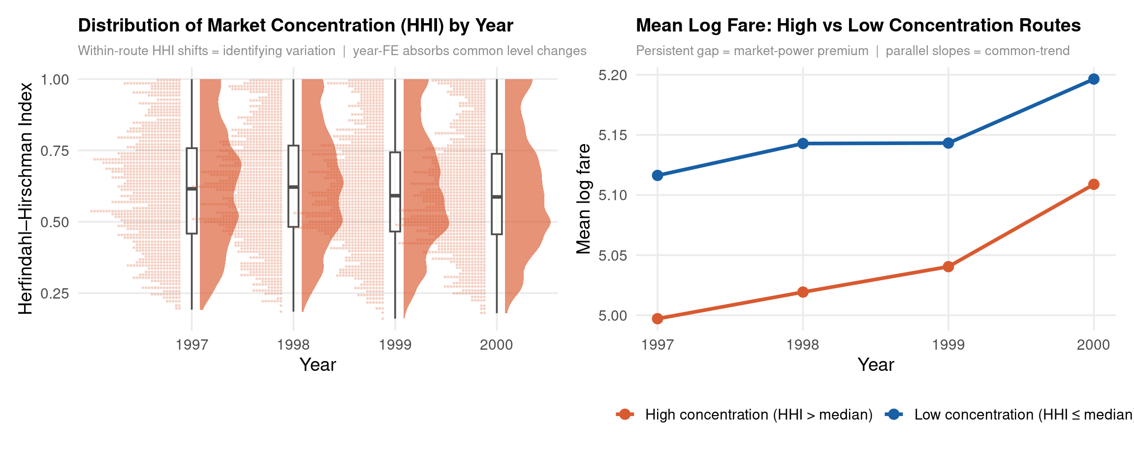
Do more concentrated airline routes have higher fares? Cross-sectional OLS confounds route-level cost differences (distance, hub dominance) with the concentration effect. TWFE exploits within-route variation in concentration over time — cleanly identifying the pricing effect of market power.

Data description

Feature	Value
Source	Wooldridge airfare dataset
Units	1,149 airline routes
Periods	4 years (1997–2000)
Outcome	lfare — log average fare
Key regressors	concen (Herfindahl index), ldist (log distance)

Estimation strategy

\[\log(\text{fare}_{it}) = \alpha_i + \lambda_t + \beta_c \,\text{concen}_{it} + \varepsilon_{it}\]

• \(\alpha_i\) (route FE): baseline cost structure, hub geography, competitive landscape
• \(\lambda_t\) (year FE): jet fuel prices, deregulation waves, macroeconomic conditions

Tip

ldist is time-invariant (distance doesn’t change) → absorbed by route FE. Only concen and year dummies are identified.

Example 3: airfare — Diagnostics

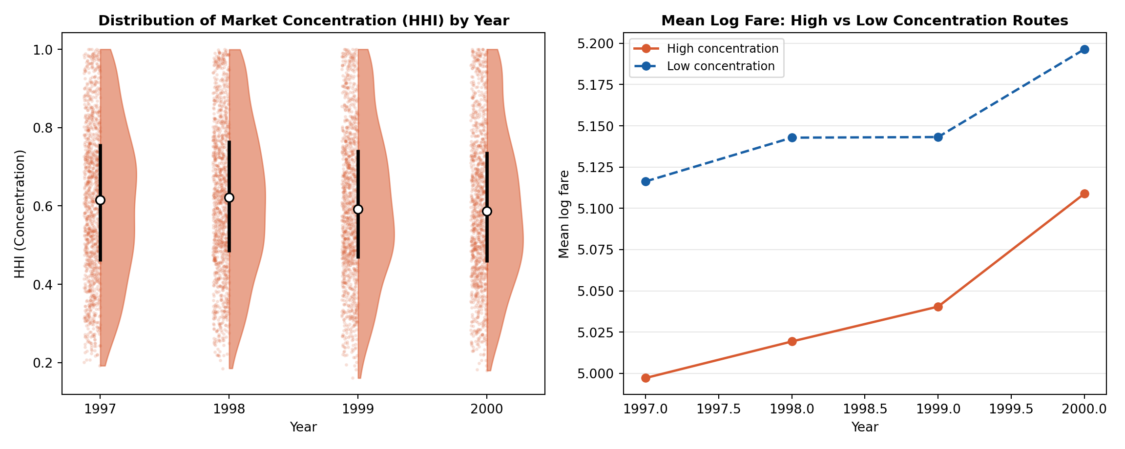
Two plots motivate identification: (1) does market concentration (HHI) vary enough within routes over time to provide identifying variation? (2) do high- and low-concentration routes show parallel fare trends before deregulation effects kick in?

library(ggdist)
data("airfare", package = "wooldridge")
pdf_a  <- pdata.frame(airfare, index = c("id","year"))

# ── Plot 1: raincloud of HHI concentration by year ───────────────────────────
# Half-violin + dots + IQR shows the full distribution of HHI across routes.
# If the distribution barely shifts year-to-year, within-route variation is
# limited and identification is weak. Visible movement = credible design.
p1 <- airfare %>%
  mutate(yr = factor(year)) %>%
  ggplot(aes(x = yr, y = concen, fill = yr, colour = yr)) +
  stat_halfeye(adjust = 0.6, width = 0.5, justification = -0.18,
               .width = 0, point_colour = NA, alpha = 0.65) +
  geom_boxplot(width = 0.1, outlier.shape = NA,
               fill = "white", alpha = 0.7, colour = "grey30") +
  stat_dots(side = "left", justification = 1.12, binwidth = NA, overflow = "compress", alpha = 0.18) +
  scale_fill_manual(values   = rep(col_accent, 4), guide = "none") +
  scale_colour_manual(values = rep(col_accent, 4), guide = "none") +
  labs(title    = "Distribution of Market Concentration (HHI) by Year",
       subtitle = "Within-route HHI shifts = identifying variation  |  year-FE absorbs common level changes",
       x = "Year", y = "Herfindahl–Hirschman Index") +
  theme(plot.subtitle = element_text(size = 10, colour = col_muted))

# ── Plot 2: mean log fare by concentration group over time ───────────────────
# Routes above median first-year HHI = "high concentration".
# A persistent level gap confirms the market-power price premium;
# parallel slopes across years validate the common-trend assumption.
med_hhi_yr1 <- airfare %>% filter(year == min(year)) %>% pull(concen) %>% median()
airfare_grp <- airfare %>%
  group_by(id) %>%
  mutate(hi = concen[year == min(year)] > med_hhi_yr1) %>%
  ungroup() %>%
  mutate(grp = if_else(hi, "High concentration (HHI > median)",
                           "Low concentration (HHI ≤ median)")) %>%
  group_by(grp, year) %>%
  summarise(mean_lfare = mean(lfare), .groups = "drop")

p2 <- airfare_grp %>%
  ggplot(aes(x = year, y = mean_lfare, colour = grp, group = grp)) +
  geom_line(linewidth = 1.3) + geom_point(size = 3.2) +
  scale_colour_manual(values = c(col_accent, col_main)) +
  labs(title    = "Mean Log Fare: High vs Low Concentration Routes",
       subtitle = "Persistent gap = market-power premium  |  parallel slopes = common-trend",
       x = "Year", y = "Mean log fare", colour = NULL) +
  theme(legend.position  = "bottom",
        plot.subtitle    = element_text(size = 10, colour = col_muted))

p1 + p2

import pandas as pd, numpy as np, matplotlib.pyplot as plt
from scipy.stats import gaussian_kde

def raincloud(ax, arr, pos, color, width=0.28, dot_alpha=0.12, dot_size=3):
    arr = np.asarray(arr)[~np.isnan(np.asarray(arr))]
    kde   = gaussian_kde(arr, bw_method=0.28)
    ygrid = np.linspace(arr.min(), arr.max(), 200)
    xkde  = kde(ygrid) / kde(ygrid).max() * width
    ax.fill_betweenx(ygrid, pos, pos + xkde, alpha=0.55, color=color);
    jit = np.random.uniform(-width * 0.45, 0, len(arr))
    ax.scatter(pos + jit, arr, alpha=dot_alpha, s=dot_size, color=color, zorder=2);
    q25, med, q75 = np.percentile(arr, [25, 50, 75])
    ax.vlines(pos, q25, q75, color="k", linewidth=2.5, zorder=3);
    ax.scatter(pos, med, color="white", s=45, zorder=4,
               edgecolors="k", linewidth=1.2);

# ── Data ──────────────────────────────────────────────────────────────────────
air = pd.read_csv("https://vincentarelbundock.github.io/Rdatasets/csv/wooldridge/airfare.csv")
air = air.dropna(subset=["lfare","concen"])

np.random.seed(14159)
fig, axes = plt.subplots(1, 2, figsize=(12, 4.8))

# ── Plot 1: raincloud of HHI by year ─────────────────────────────────────────
# Each raincloud shows the route HHI distribution for one year.
# Visible year-to-year movement in the body of the distribution confirms
# there is within-route concentration variation for TWFE to exploit.
years_a = sorted(air["year"].unique())
for i, yr in enumerate(years_a):
    raincloud(axes[0], air.loc[air["year"]==yr, "concen"], i, "#D85A30")
axes[0].set_xticks(range(len(years_a))); axes[0].set_xticklabels(years_a);
axes[0].set_xlabel("Year"); axes[0].set_ylabel("HHI (Concentration)");
axes[0].set_title("Distribution of Market Concentration (HHI) by Year",
                  fontsize=11, fontweight="bold");

# ── Plot 2: mean log fare by concentration group ──────────────────────────────
# Routes above/below median first-year HHI compared over time.
# Parallel slopes validate common trends; the level gap confirms the premium.
yr0 = air["year"].min()
med_hhi = air[air["year"]==yr0]["concen"].median()
grp_map = (air[air["year"]==yr0].set_index("id")["concen"] > med_hhi) \
            .map({True:"High concentration", False:"Low concentration"})
air["grp"] = air["id"].map(grp_map)
for grp, col, ls in [("High concentration","#D85A30","-"),
                      ("Low concentration", "#185FA5","--")]:
    mn = air[air["grp"]==grp].groupby("year")["lfare"].mean()
    axes[1].plot(mn.index, mn.values, marker="o", color=col,
                 linestyle=ls, linewidth=1.8, label=grp);
axes[1].set_xlabel("Year"); axes[1].set_ylabel("Mean log fare");
axes[1].set_title("Mean Log Fare: High vs Low Concentration Routes",
                  fontsize=11, fontweight="bold");
axes[1].legend(fontsize=9); axes[1].grid(axis="y", alpha=0.3);
plt.tight_layout(); plt.show()

use "http://fmwww.bc.edu/ec-p/data/wooldridge/airfare.dta", clear
quietly xtset id year

* ── Plot 1: distribution of HHI by year ──────────────────────────────────────
* Box plot of route HHI by year. Any visible shift means the year FE
* absorbs aggregate concentration trends; within-route variation
* (the identifying signal) remains after double-demeaning.
graph box concen, over(year) ///
    box(1, fcolor(orange_red%40) lcolor(orange_red)) ///
    title("Distribution of Market Concentration (HHI) by Year") ytitle("HHI")
cap mkdir plots
 quietly graph export "../plots/airfare-diag1-stata.png", replace width(800)

* ── Plot 2: mean log fare by concentration group ─────────────────────────────
* Routes above median first-year HHI = high concentration.
* Parallel trends validate common-trend; persistent level gap = market-power premium.
preserve
quietly summarize concen if year == 1997, detail
gen hi = (concen > r(p50)) if year == 1997
bysort id: replace hi = hi[1]
drop if missing(hi)
collapse (mean) mean_lfare = lfare, by(hi year)
twoway (line mean_lfare year if hi==1, lcolor(orange_red) lwidth(medthick)) ///
       (line mean_lfare year if hi==0, lcolor(navy) lwidth(medthick) lpattern(dash)), ///
    legend(order(1 "High concentration" 2 "Low concentration") rows(1)) ///
    title("Mean Log Fare: High vs Low Concentration Routes") ///
    xtitle("Year") ytitle("Mean log fare")
 quietly graph export "../plots/airfare-diag2-stata.png", replace width(800)
restore

(3,447 missing values generated)

(3,447 real changes made)

(0 observations deleted)

Example 3: airfare — Estimation & Results

ols_a  <- lm(lfare ~ concen + ldist + y98 + y99 + y00, data = airfare)
fe_a   <- plm(lfare ~ concen, data = pdf_a, model = "within", effect = "individual")
twfe_a <- feols(lfare ~ concen | id + year, data = airfare, cluster = ~id)
modelsummary(
  list("Pooled OLS" = ols_a, "Route FE" = fe_a, "TWFE" = twfe_a),
  coef_map = c("concen"="Concentration (HHI)","ldist"="Log distance",
               "y98"="Year 1998","y99"="Year 1999","y00"="Year 2000"),
  stars = TRUE, gof_omit = "IC|Log|RMSE",
  title = "Airline Fares: Effect of Market Concentration (1997–2000)"
)

Airline Fares: Effect of Market Concentration (1997–2000)

	Pooled OLS	Route FE	TWFE
+ p < 0.1, * p < 0.05, ** p < 0.01, *** p < 0.001
Concentration (HHI)	0.324***	0.103***	0.169***
	(0.030)	(0.031)	(0.049)
Log distance	0.454***
	(0.009)
Year 1998	0.021
	(0.014)
Year 1999	0.038**
	(0.014)
Year 2000	0.099***
	(0.014)
Num.Obs.	4596	4596	4596
R2	0.392	0.003	0.955
R2 Adj.	0.391	-0.329	0.940
R2 Within			0.009
R2 Within Adj.			0.009
F	591.049
FE: id			X
FE: year			X

import pandas as pd, numpy as np, pyfixest as pf

air2 = pd.read_csv("https://vincentarelbundock.github.io/Rdatasets/csv/wooldridge/airfare.csv")
air2 = air2.dropna(subset=["lfare","concen","ldist"])

ols_a_py  = pf.feols("lfare ~ concen + ldist + y98 + y99 + y00", data=air2)
twfe_a_py = pf.feols("lfare ~ concen | id + year", data=air2, vcov={"CRV1":"id"})

def _stars(p): return "***" if p<.01 else "**" if p<.05 else "*" if p<.10 else ""
for label, m in [("Pooled OLS", ols_a_py), ("TWFE", twfe_a_py)]:
    print(f"\n{label}")
    for v in ["concen","ldist"]:
        if v in m.coef().index:
            c, s, p = m.coef()[v], m.se()[v], m.pvalue()[v]
            print(f"  {v:10} {c:8.4f}{_stars(p):4}  ({s:.4f})")

Pooled OLS
  concen       0.3239***   (0.0302)
  ldist        0.4539***   (0.0090)

TWFE
  concen       0.1689***   (0.0495)

use "http://fmwww.bc.edu/ec-p/data/wooldridge/airfare.dta", clear
quietly xtset id year
quietly regress lfare concen ldist y98 y99 y00
quietly estimates store OLS_a
quietly xtreg lfare concen, fe
quietly estimates store FE_a
cap ssc install require, replace
quietly reghdfe lfare concen, absorb(id year) vce(cluster id)
quietly estimates store TWFE_a
esttab OLS_a FE_a TWFE_a, b(4) se(4) star(* 0.10 ** 0.05 *** 0.01) ///
    keep(concen ldist y98 y99 y00) mtitles("Pooled OLS" "Route FE" "TWFE") ///
    title("Airline Fares: Concentration Effect")

Airline Fares: Concentration Effect
------------------------------------------------------------
                      (1)             (2)             (3)   
               Pooled OLS        Route FE            TWFE   
------------------------------------------------------------
concen             0.3239***       0.1031***       0.1689***
                 (0.0302)        (0.0312)        (0.0495)   

ldist              0.4539***                                
                 (0.0090)                                   

y98                0.0214                                   
                 (0.0142)                                   

y99                0.0376***                                
                 (0.0142)                                   

y00                0.0995***                                
                 (0.0142)                                   
------------------------------------------------------------
N                    4596            4596            4596   
------------------------------------------------------------
Standard errors in parentheses
* p<0.10, ** p<0.05, *** p<0.01

Example 3: airfare — Interpretation & Summary

\[\widehat{\log(\text{fare})}^{OLS}_{it} = \underset{}{0.324}\,\text{concen}_{it} + \underset{}{0.454}\,\log(\text{dist})_{i} + \ldots\]

\[\widehat{\log(\text{fare})}^{TWFE}_{it} = \underset{}{0.169}\,\text{concen}_{it} + \alpha_i + \lambda_t \quad\checkmark\]

Interpretation. Moving from a perfectly competitive route (HHI = 0) to a monopoly route (HHI = 1) is associated with a fare increase of approximately 18.4% (\(e^{0.169}-1\)), holding route characteristics and year shocks constant. The OLS estimate is larger in magnitude, reflecting the confounding effect of route distance and hub geography on both fares and concentration.

Summary across all three examples:

Example	Entity	Time	Key finding
crime4	County	Year	Deterrence reduces crime; OLS confounded by county culture
wagepan	Individual	Year	Union premium ≈10%; OLS overstates due to ability selection
airfare	Route	Year	Concentration raises fares ≈20%; distance confounding in OLS

Exercises — Estimation

1. Extend the DGP to include heterogeneous treatment effects: set \(\beta_i = 2 + 0.5\cdot\alpha_i\) (larger effects for high-FE units). Re-estimate with TWFE. Is \(\hat{\beta}^{TWFE}\) close to \(\bar{\beta} = 2\)? Why or why not?

2. Add a covariate endogenous to time: generate \(z_{it} = \lambda_t + w_{it}\) (correlated with the time FE). Show that entity-only FE is biased for \(z\)’s effect but TWFE is not.

3. Compare estimators on crime4: estimate three specifications — (a) entity FE only, (b) time FE only, (c) TWFE — and produce a coefficient plot comparing prbarr across specifications. Interpret any differences.

4. wagepan robustness: replicate the union wage premium using (a) first differences, (b) TWFE, and (c) the Mundlak correction. Compare estimates and discuss which identification strategy is most credible.

5. airfare event study: create a relative-time variable based on entry/exit of a low-cost carrier (use y98–y00 as pseudo-events). Run an event study specification and test for pre-trends.

Exercises — Testing

1. Simulate under \(H_0\) for F-tests: set all \(\lambda_t = 0\) in the DGP. Re-run the F-test for time FE. Does the test correctly fail to reject? Repeat 500 times and plot the empirical distribution of the \(F\)-statistic against \(F(9, 1791)\).

2. Serial correlation in crime4: run the Wooldridge test (xtserial / pbgtest) on the crime4 TWFE residuals. Compare the TWFE coefficients under iid SEs vs. clustered SEs. How large is the difference in standard errors?

3. Test for time FE on wagepan: the NLSY panel (1980–1987) spans a period of significant macro shifts (recessions, wage compression). Formally test whether year dummies are jointly significant. Interpret the result in terms of identification.

4. Bacon decomposition on wagepan: union status changes within individuals over time — a staggered adoption setting. Perform a Bacon decomposition. Are any 2×2 weights negative? What does this imply for the aggregate TWFE estimate?

5. Callaway-Sant’Anna vs TWFE on crime4: construct a first-treated year for each county (assume treatment is the introduction of a policing program at different times). Compare the simple aggregate ATT from CS to the TWFE estimate.

Further Reading

Textbooks

• Baltagi (2021) — Econometric Analysis of Panel Data, 6th ed. Springer. Chapters 3–5: TWFE, error components, robust inference.

• Wooldridge (2010) — Econometric Analysis of Cross Section and Panel Data, 2nd ed. MIT Press. Chapter 10: unobserved effects, FE, FD.

• Angrist & Pischke (2009) — Mostly Harmless Econometrics. Princeton. Chapter 5: IV/DiD, event study.

• Cunningham (2021) — Causal Inference: The Mixtape. Yale. Chapters 8–9: DiD and TWFE. Free: mixtape.scunning.com

• Huntington-Klein (2022) — The Effect. CRC Press. Panel methods chapter. Free: theeffectbook.net

Key articles — TWFE critique

• Goodman-Bacon (2021). JOE 225(2): 254–277.
• Callaway & Sant’Anna (2021). JOE 225(2): 200–230.
• Sun & Abraham (2021). JOE 225(2): 175–199.
• de Chaisemartin & D’Haultfœuille (2020). AER 110(9): 2964–2996.
• Borusyak, Jaravel & Spiess (2024). ReStud 91(6): 3253–3285.
• Roth, Sant’Anna, Bilinski & Poe (2023). JOE 235(2): 2218–2244.
• Wooldridge (2025). Empirical Economics 69(5): 2545–2587.

Online resources

• Andrew Baker’s TWFE resources: andrewcbaker.netlify.app
• Pedro Sant’Anna’s DiD notes: pedrohcgs.github.io
• Nick Huntington-Klein’s DiD guide on did2s, csdid, etc.

Software documentation

• fixest (R): L. Bergé. doi:10.32614/CRAN.package.fixest · lrberge.github.io/fixest
• pyfixest (Py): s3alfisc.github.io/pyfixest
• did (R): Callaway & Sant’Anna. doi:10.32614/CRAN.package.did · bcallaway11.github.io/did
• Stata reghdfe: Correia (2017). scorreia.com/software/reghdfe

Journals

Journal of Econometrics · Econometrica · Review of Economics & Statistics · American Economic Review

Thank You

Athanassios Stavrakoudis
Applied Informatics and Computational Economics Lab
Department of Economics
University of Ioannina, Greece

astavrak@uoi.gr · linkedin.com/in/astavrakoudis