import pandas as pd, numpy as npimport statsmodels.api as sm # OLS / WLS with robust SEfrom linearmodels.iv import IV2SLS # fuzzy RDD# rdrobust is also available on PyPI (import rdrobust)
ssc install rdrobust // rdrobust, rdbwselect, rdplotssc install rddensity // manipulation test + rdplotdensityssc install lpdensity // dependency of rddensity* Fuzzy RDD uses built-in ivregress 2sls (no extra install)
Note
Two views, on purpose. The cross-language estimation slides are hand-coded (local-linear WLS, plain OLS/2SLS) so every language returns the same numbers to the digit and you can see exactly what the software does. The specialised tooling slides then run rdrobust (MSE-optimal bandwidth + robust bias-corrected CI) and rddensity (formal manipulation test) live in R, Python and Stata — and those agree across languages too (\(\hat\tau = -2.41\), robust \(p = 0.042\)).
In observational data, treatment is rarely exogenous — the treated differ from the untreated in unobserved ways. RDD exploits a special situation: treatment is switched on/off by a threshold crossing rule on an observable running variable\(X\).
Just below vs just above the cut-off \(c\), units are almost identical — the only systematic difference is treatment.
Assignment near \(c\) is “as good as random” (Lee 2008): units cannot perfectly control which side they land on.
So a jump in the outcome at \(c\) is a causal effect — no unconfoundedness assumption on covariates needed.
Any rule of the form “you get treatment if a score passes a threshold”:
Elections — incumbency advantage: win if vote share \(> 50\%\).
Potential outcomes \(Y_0\) (untreated) and \(Y_1\) (treated). The individual treatment effect is \(\theta = Y_1 - Y_0\) (random). The conditional ATE given the running variable is
We target the ATE at the cut-off — the subpopulation affected at the margin by the policy:
\[\bar\theta = \theta(c) = \mathbb{E}[\theta \mid X = c].\]
This is a narrowly-defined but policy-relevant parameter: the effect of nudging the threshold.
With \(m_0(x)\) observed only for \(x<c\) and \(m_1(x)\) only for \(x\ge c\), using \(\bar\theta\) for other \(x\) is extrapolation.
Note
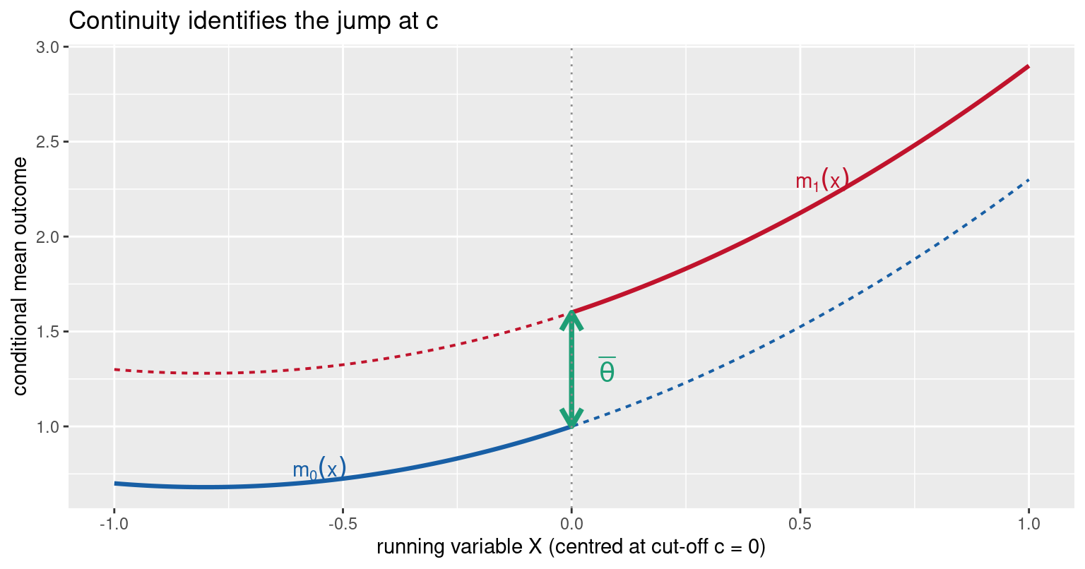
Head Start reading.\(m_0(x)\) = mortality if a county gets no grant-writing help; \(m_1(x)\) = mortality with help. Both are smooth functions of the 1960 poverty rate. There is no reason for either to jump at \(59.2\%\) — so any jump in observed mortality there is the causal effect of the programme.
Continuity of Potential Outcomes
The identifying assumption
A randomized experiment makes (Y_0, Y_1) independent of treatment. RDD asks for much less: only that the two potential-outcome regressions are continuous at the single point (x=c).
Continuity says the counterfactual trend would have passed smoothly through the cut-off. Anything discrete you see at (c) must therefore be the treatment — because nothing else is allowed to jump there.
This is weaker than unconfoundedness (no need to control for covariates) and local (it only constrains behaviour at (c)), which is exactly why RDD identifies an effect only at the cut-off.
# Two smooth potential-outcome regressions. We observe m0 only left of c and# m1 only right of c (solid); their counterfactual continuations are dashed.# The identified effect is the vertical jump at c — nothing else moves there.x <-seq(-1, 1, length.out =400)m0 <-1.0+0.8* x +0.5* x^2# E[Y0 | X=x]m1 <-1.6+0.8* x +0.5* x^2# E[Y1 | X=x], jump = 0.6 at cdf <-data.frame(x, m0, m1)ggplot(df, aes(x)) +geom_line(aes(y = m0), linewidth =1.1, colour ="#185FA5",data =subset(df, x <0)) +geom_line(aes(y = m1), linewidth =1.1, colour ="#C0132C",data =subset(df, x >=0)) +geom_line(aes(y = m0), linewidth =0.7, colour ="#185FA5",linetype ="22", data =subset(df, x >=0)) +geom_line(aes(y = m1), linewidth =0.7, colour ="#C0132C",linetype ="22", data =subset(df, x <0)) +annotate("segment", x =0, xend =0, y =1.0, yend =1.6,colour ="#1D9E75", linewidth =1.3,arrow =arrow(ends ="both", length =unit(0.15, "in"))) +annotate("text", x =0.06, y =1.3, hjust =0, colour ="#1D9E75",fontface ="bold", label ="theta-bar") +geom_vline(xintercept =0, linetype ="dotted", colour ="grey55") +labs(x ="running variable X (centred at cut-off c = 0)",y ="conditional mean outcome",title ="Continuity identifies the jump at c")
Solid curves are observed (each potential outcome is seen only on its own side); dashed curves are the counterfactual continuations we never see. Continuity says the dashed pieces join the solid ones smoothly — so the only break at \(c\) is the green jump \(\bar\theta\).
The identifying assumption is a statement about the two regression functions, not about independence:
\[m_0(x) = \mathbb{E}[Y_0 \mid X = x], \qquad m_1(x) = \mathbb{E}[Y_1 \mid X = x]\]
are continuous at \(x = c\). Equivalently, the left and right limits of each exist and agree with the function value:
The assumptions look similar but live in different dimensions:
DiD compares the same units over time and assumes their untreated path would have moved parallel to a control group — an assumption about trends across time.
RDD compares different units at one instant just either side of \(c\) and assumes their outcome regressions are smooth in the score — an assumption about continuity across \(X\).
Note
RDD is often described as “IV-like” at the cut-off. In the fuzzy design (later), the threshold indicator \(Z = \mathbb{1}\{X \ge c\}\) is literally used as an instrument for actual treatment \(D\), and the estimand becomes a LATE for compliers at \(c\). Sharp RDD is the special case of perfect compliance.
A hard threshold rule assigns treatment \(\Rightarrow\) reach for RDD.
A policy switches on at a date for some groups \(\Rightarrow\)DiD.
An exogenous shifter nudges an endogenous treatment \(\Rightarrow\)IV.
RDD buys the weakest, most local assumption — at the cost of a local, less generalizable estimand.
Identification — Theorem 21.1
Proof of Theorem 21.1
Write the observed conditional mean by conditioning the observed outcome on (X=x):
[ m(x) = m_0(x),{x<c} + m_1(x),{xc}. ]
Take right and left limits at (c). Since (m_0) and (m_1) are continuous at (c):
The conditional mean (m(x)) is generically identified from data, hence so is the jump — and therefore ().
A Local Parameter
RDD identifies the ATE only at (X=c). In Head Start terms, () is the effect for a county with a (59%) poverty rate — not for a (30%) county. Using () elsewhere is extrapolation.
Nonparametric estimation is essential. If you force a parametric (e.g. linear) fit on each side, the best-fitting lines will generically show a jump at (c) even when the true (m(x)) is continuous — you would mistake curvature for a discontinuity. This is why local linear regression (small bandwidth) is preferred over global polynomials.
Covariates are not needed for identification (continuity does the work). They can, however, shrink the residual variance and improve precision — see the covariates slide.
Let \(m(x) = \mathbb{E}[Y \mid X = x]\) and \(m(c{\pm}) = \lim_{z \to c^{\pm}} m(z)\).
Theorem 21.1 (Hahn, Todd & Van der Klaauw 2001). Assume \(D = \mathbb{1}\{X \ge c\}\) and that \(m_0(x)\) and \(m_1(x)\) are continuous at \(x = c\). Then \[\boxed{\;\bar\theta = m(c{+}) - m(c{-})\;}\]
The RDD treatment effect is the vertical jump in the conditional mean at the cut-off. That is the whole idea — estimation reduces to estimating two boundary points.
The conditions are minimal — no unconfoundedness, no functional form:
Continuity of \(m_0(\cdot)\) and \(m_1(\cdot)\) at \(c\): absent treatment, the outcome would evolve smoothly through \(c\).
No manipulation: units cannot precisely sort across \(c\) (testable — density test).
No coincident treatments: nothing else switches at \(c\).
Continuity is an assumption about the counterfactual\(m_0\) at \(c^+\) and \(m_1\) at \(c^-\) — inherently untestable, but supported by placebo checks.
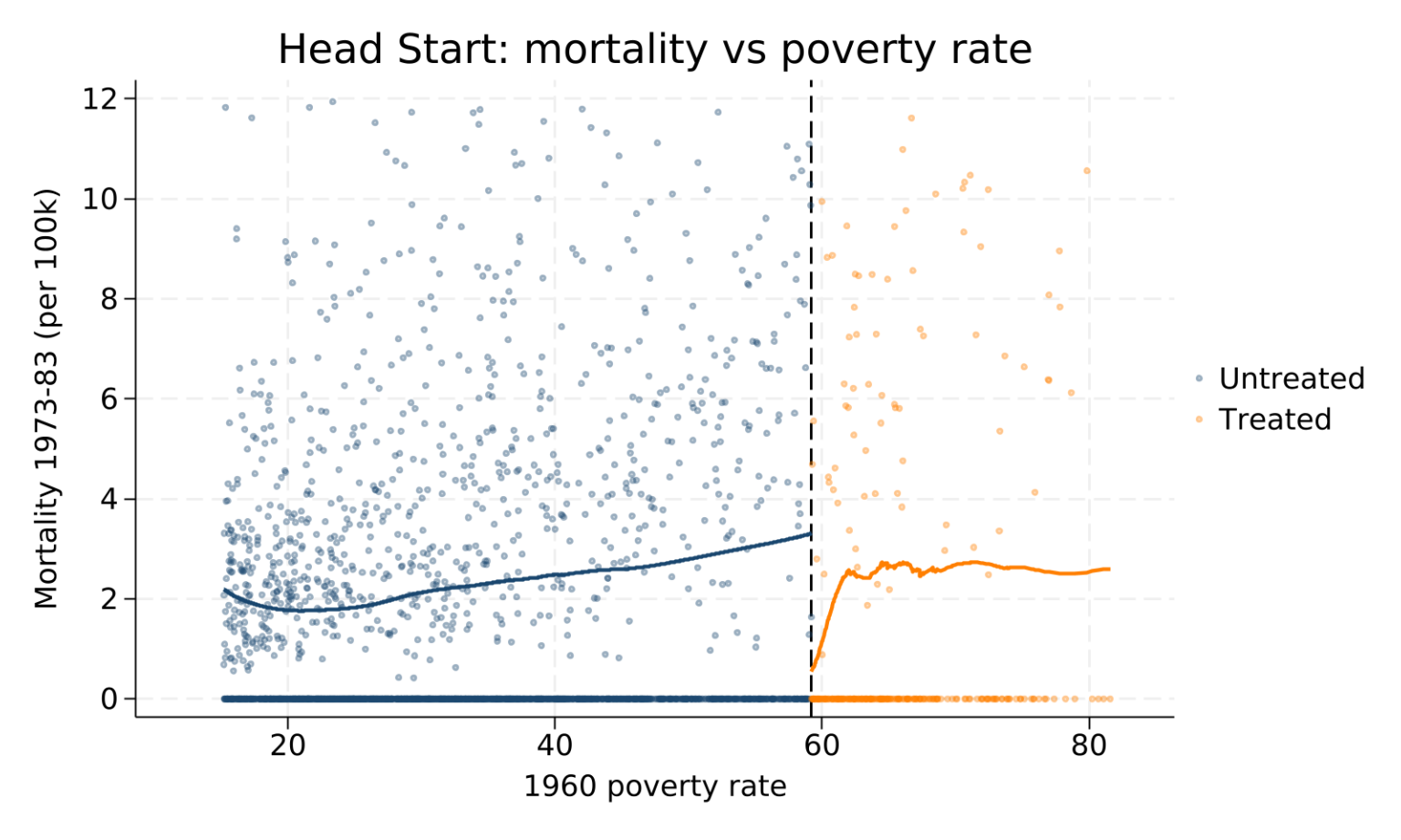
import delimited "../data/rdd-headstart.csv", case(preserve) clearscalar C0 = 59.1984gen treated = povrate60 >= C0* Scatter + lowess smoother each side, saved to a temp PNG (../plots/).* Same axes and smoother as the R/Python tabs for a like-for-like picture.* Scatter is clipped to mortHS<=12 to match R/Python's clipped VIEW; the lowess* is computed on ALL data (asin R/Python), so the smoother is identical.twoway (scatter mortHS povrate60 if !treated & mortHS<=12, msize(vsmall) mcolor(navy%25)) /// (scatter mortHS povrate60 if treated & mortHS<=12, msize(vsmall) mcolor(orange%25)) /// (lowess mortHS povrate60 if !treated, lcolor(navy) lwidth(medthick) bwidth(0.6)) /// (lowess mortHS povrate60 if treated, lcolor(orange) lwidth(medthick) bwidth(0.6)), ///xline(59.1984, lpattern(dash)) ///xscale(range(10 85)) xlabel(20(20)80) ///yscale(range(0 12)) ylabel(0(2)12) ///legend(order(1 "Untreated" 2 "Treated")) ///xtitle("1960 poverty rate") ytitle("Mortality 1973-83 (per 100k)") ///title("Head Start: mortality vs poverty rate")graphexport"../plots/rdd_stata_data.png", replacewidth(1600)
Note
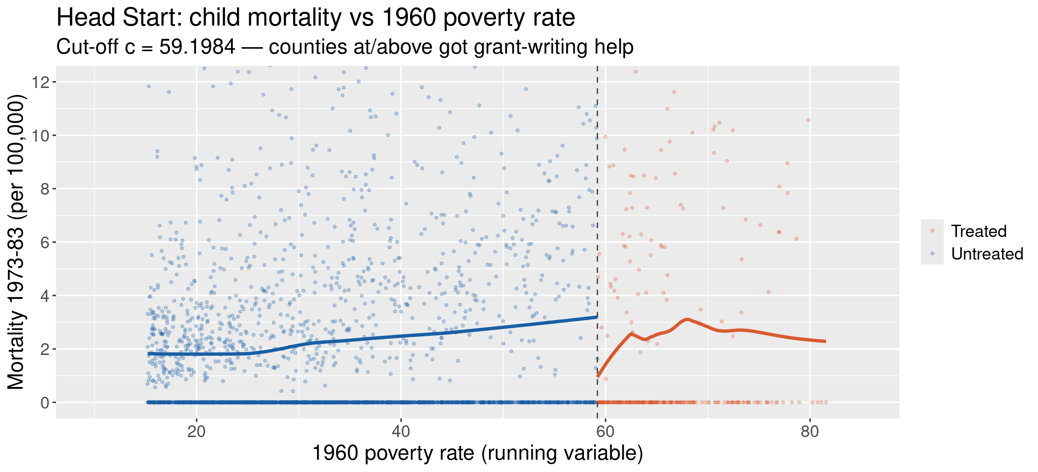
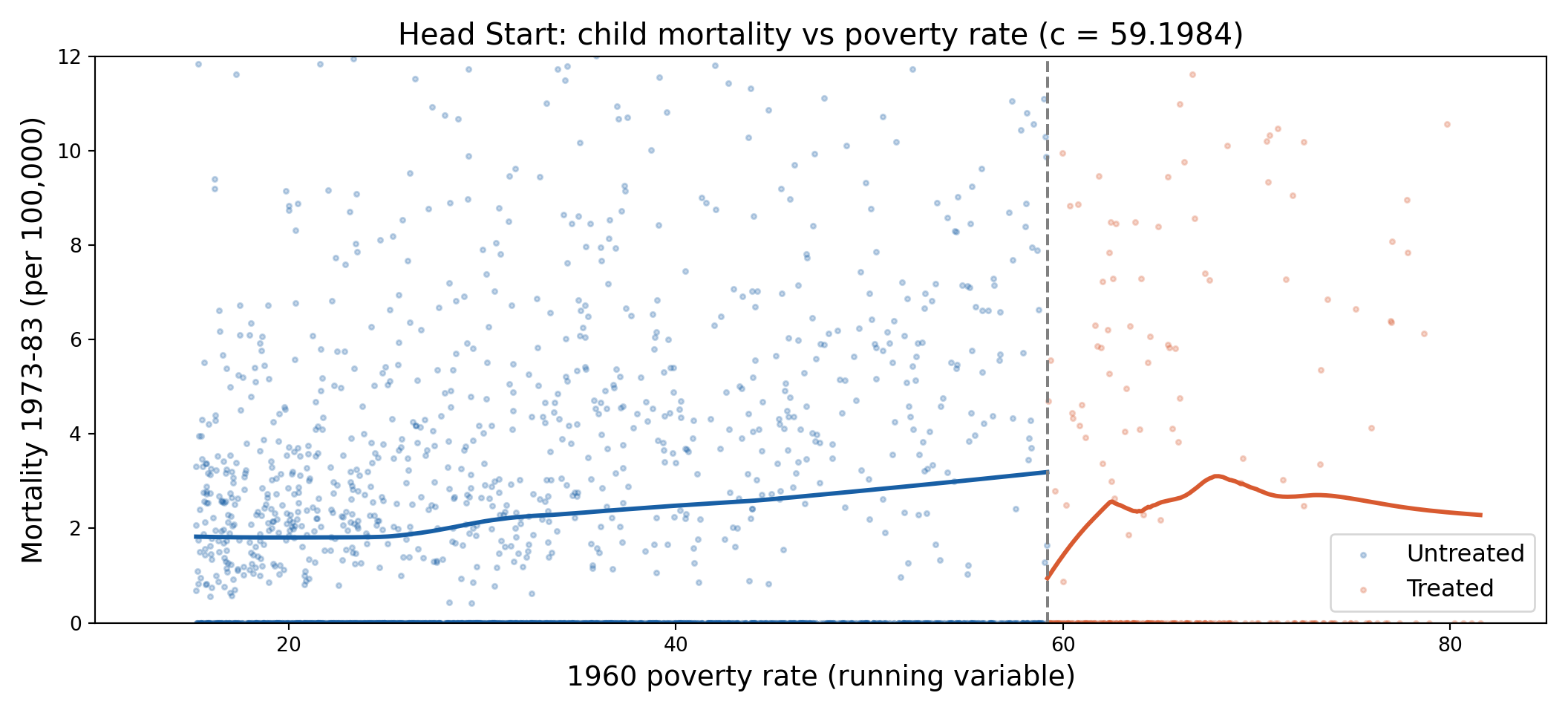
What to observe. Mortality rises with poverty (both sides) and drops downward just above the cut-off — exactly the treatment signature. Density thins out at high poverty (few counties), so the treated side is estimated with more noise. The raw scatter is very disperse; the discontinuity is a property of the conditional mean, not the raw cloud.
Part II — Estimation
Local Linear Estimation
Boundary Estimation
The RDD estimand needs (m(x)) exactly at the boundary (x=c). The Nadaraya-Watson (local constant) estimator is biased at a boundary point — it averages points that lie only on one side, so its bias is (O(h)) rather than (O(h^2)).
Series / global polynomial estimators have high variance at the boundary and are sensitive to points far from (c).
Local linear (LL) regression fits a line inside the bandwidth window on each side: it is boundary-adaptive, with bias (O(h^2)) and good boundary variance. This is why LL is the workhorse of modern RDD (Hansen §19.4, §19.10).
Gelman & Imbens (2019)
Fitting a high-order global polynomial ((x, x^2, , x^p)) over the whole support is a common but bad habit:
Weights on observations become erratic — far-away points drive the estimate at (c).
Estimates and confidence intervals are extremely sensitive to the polynomial order (p).
Runge-type oscillation near the boundary manufactures spurious discontinuities.
Recommendation: local linear (or local quadratic) with a small bandwidth. Report robustness to the bandwidth, not to the polynomial order.
The triangular kernel \(K(u) = (1-|u|)\mathbb{1}\{|u|\le 1\}\) is optimal at a boundary. Equivalently, a single weighted regression on all \(|X-c|\le h\) gives \(\hat{\bar\theta}\) directly as the coefficient on \(D\):
hs_df <-read.csv("../data/rdd-headstart.csv"); C0 <-59.1984; h <-8# One weighted regression with a triangular kernel. theta = coefficient on D.xx <- hs_df$povrate60 - C0D <-as.numeric(hs_df$povrate60 >= C0)k <-pmax(0, 1-abs(xx) / h) # triangular weights, support |X-c| <= hfit <-lm(mortHS ~ xx + D + xx:D, data = hs_df, weights = k)# CAREFUL: vcovHC() on a weighted lm treats k as VARIANCE weights (wrong here).# Build the kernel-weighted robust sandwich by hand (HC1):use <- k >0Z <-cbind(1, xx, D, xx * D)[use, ]y <- hs_df$mortHS[use]; kk <- k[use]; n <-nrow(Z)bread <-solve(t(Z * kk) %*% Z)e <-as.numeric(y - Z %*%coef(fit))meat <-t(Z * (kk^2* e^2)) %*% ZV <- bread %*% meat %*% bread * (n / (n -4))theta <-coef(fit)["D"]; se <-sqrt(V[3, 3])cat(sprintf("Local linear (triangular, h=%d): theta = %.4f se = %.4f t = %.2f\n", h, theta, se, theta / se))
Local linear RDD — Head Start (triangular kernel, h = 8)
theta_hat = -2.2487 se = 1.0763 t = -2.09 (n in window = 482)
m(c-) (untreated rate at cut-off) = 3.58 per 100,000
=> a drop of 2.2 is about 63% of the baseline mortality rate.
Code
import pandas as pd, numpy as np, statsmodels.api as smhs = pd.read_csv("../data/rdd-headstart.csv"); C0 =59.1984; h =8xx = hs.povrate60.values - C0D = (hs.povrate60.values >= C0).astype(float)k = np.maximum(0, 1- np.abs(xx) / h) # triangular weightsZ = np.column_stack([np.ones_like(xx), xx, D, xx * D])use = k >0# WLS with HC1 robust SE reproduces the kernel-weighted sandwich exactly.fit = sm.WLS(hs.mortHS.values[use], Z[use], weights=k[use]).fit(cov_type="HC1")theta, se = fit.params[2], fit.bse[2]print(f"Local linear (triangular, h={h}): theta = {theta:.4f} se = {se:.4f} t = {theta/se:.2f}")
Local linear (triangular, h=8): theta = -2.2487 se = 1.0763 t = -2.09
Code
print(f"n in window = {int(use.sum())}")
n in window = 482
Code
import delimited "../data/rdd-headstart.csv", case(preserve) clearscalar C0 = 59.1984gen xx = povrate60 - C0gen D = povrate60 >= C0gen xD = xx*Dgenk = max(0, 1 - abs(xx)/8) // triangular weights, h = 8* aweight + vce(robust) gives the kernel-weighted robust sandwich (HC1)regress mortHS xx D xD [aweight=k] ifk>0, vce(robust)dias txt "theta_hat = "as res _b[D] as txt " se = "as res _se[D] ///as txt " t = "as res _b[D]/_se[D]
All three languages implement the same weighted regression and the same HC1 kernel sandwich, so they agree to the digit:
Language
\(\hat{\bar\theta}\)
\(s(\hat{\bar\theta})\)
\(t\)
R
\(-2.2487\)
\(1.0763\)
\(-2.09\)
Python
\(-2.2487\)
\(1.0763\)
\(-2.09\)
Stata
\(-2.2487\)
\(1.0763\)
\(-2.09\)
Reading it. Grant-writing assistance lowered HS-related child mortality by about 2.25 per 100,000 at the cut-off. With a baseline (untreated) rate of \(\approx 3.6\), that is a **$\(60% reduction** — a large, statistically significant policy effect (\)t $).
Warning
Weights are kernel weights, not variance weights. In R, vcovHC(lm(..., weights = k)) divides by the weights again and returns a badly understated SE. Compute the sandwich by hand — or use rdrobust. Stata’s aweight+vce(robust) and Python’s WLS(...).fit(cov_type="HC1") happen to produce exactly the kernel-weighted sandwich we want.
Code — Simple RDD Estimator
The rectangular-kernel special case is one plain OLS on the window \(|X-c|\le h\) — no special software, robust SE, identical everywhere. This is Hansen’s eq. (21.4): \[Y = \beta_0 + \beta_1 X + \beta_3 (X-c)D + \bar\theta D + e,\qquad |X-c|\le h.\]
library(sandwich); library(lmtest)hs_df <-read.csv("../data/rdd-headstart.csv"); C0 <-59.1984; h <-8sub <-abs(hs_df$povrate60 - C0) <= h # rectangular windowfit <-lm(mortHS ~I(povrate60 - C0) + D +I((povrate60 - C0) * D),data =transform(hs_df, D =as.numeric(povrate60 >= C0)), subset = sub)coeftest(fit, vcov =vcovHC(fit, type ="HC1")) # theta = coef on D
Simple RDD (rectangular, h = 8, n = 482) — reproduces Hansen eq. (21.5)
Term
Coef
SE
t
p
Intercept
3.484
0.909
3.83
0.000
X - c
0.111
0.169
0.66
0.510
D (= theta)
-2.201
1.063
-2.07
0.039
(X - c)·D
0.181
0.236
0.77
0.443
Code
import pandas as pd, numpy as np, statsmodels.api as smhs = pd.read_csv("../data/rdd-headstart.csv"); C0 =59.1984; h =8x = hs.povrate60.values - C0D = (hs.povrate60.values >= C0).astype(float)sub = np.abs(x) <= hZ = np.column_stack([np.ones_like(x), x, D, x * D])[sub]fit = sm.OLS(hs.mortHS.values[sub], Z).fit(cov_type="HC1")print(f"n = {int(sub.sum())}")
n = 482
Code
print(f"theta (coef on D) = {fit.params[2]:.4f} se = {fit.bse[2]:.4f} "f"t = {fit.tvalues[2]:.2f} p = {fit.pvalues[2]:.3f}")
theta (coef on D) = -2.2006 se = 1.0628 t = -2.07 p = 0.038
Code
import delimited "../data/rdd-headstart.csv", case(preserve) clearscalar C0 = 59.1984gen x = povrate60 - C0gen D = povrate60 >= C0gen xD = x*Dregress mortHS x D xD ifabs(x)<=8, vce(robust)dias txt "theta (coef on D) = "as res _b[D] as txt " se = "as res _se[D]
Rectangular kernel, \(h=8\), \(n = 482\) counties in \([51.2, 67.2]\):
\(\hat{\bar\theta} = -2.20\) (se \(1.06\)) — identical in R, Python and Stata, and matching Hansen’s eq. (21.5) exactly.
The rectangular estimate (\(-2.20\)) is a touch larger and less precise than the triangular one (\(-2.25\), se \(1.08\)) — the triangular kernel down-weights the window edges and is more efficient.
Tip
This is the estimator to reach for when RDD software is unavailable: it is just OLS with an interaction, on a window, with robust standard errors. The only real choice is the bandwidth \(h\).
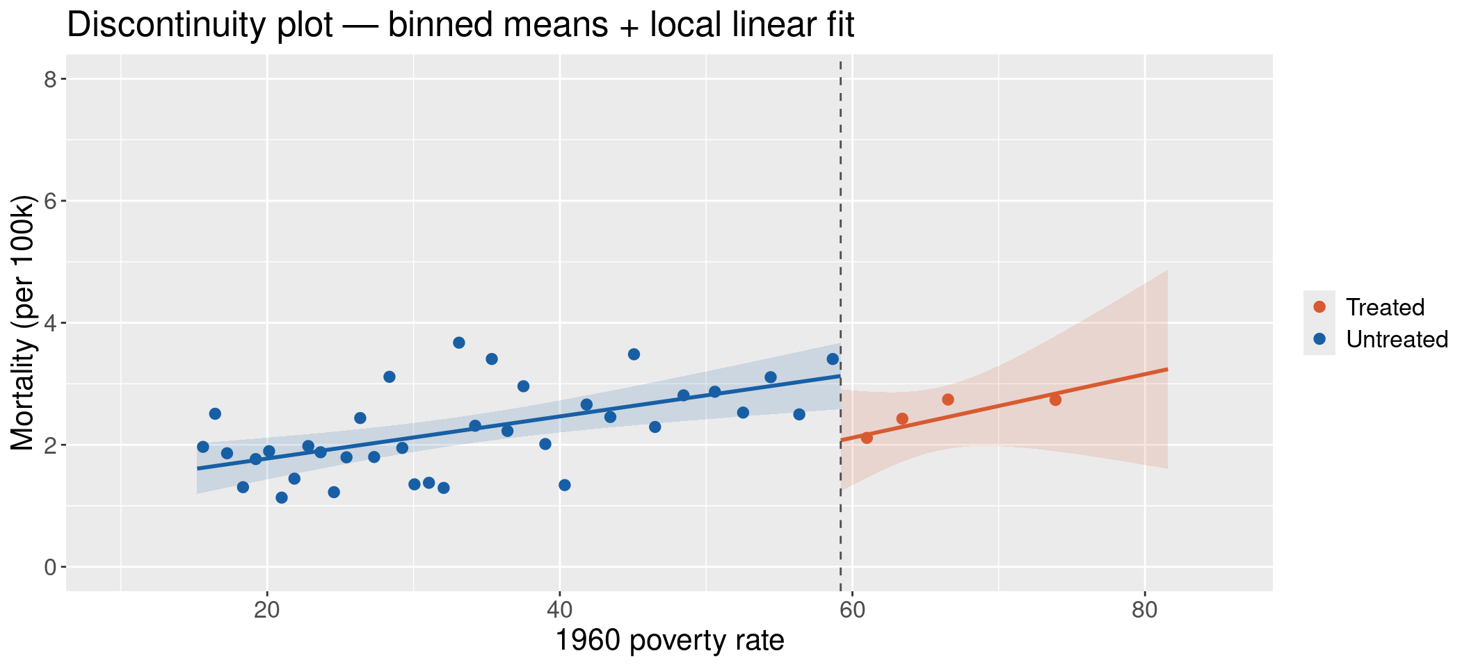
# rdplot() = binned means (equal-quantile bins) + a polynomial fit each side.# The bins are a visual aid ONLY; the estimate comes from the local-linear fit.library(rdrobust)rdplot(hs_df$mortHS, hs_df$povrate60, c = C0, p =1, nbins =c(20, 20),y.lim =c(0, 8), x.label ="1960 poverty rate", y.label ="Mortality (per 100k)",title ="rdplot — Head Start")
Code
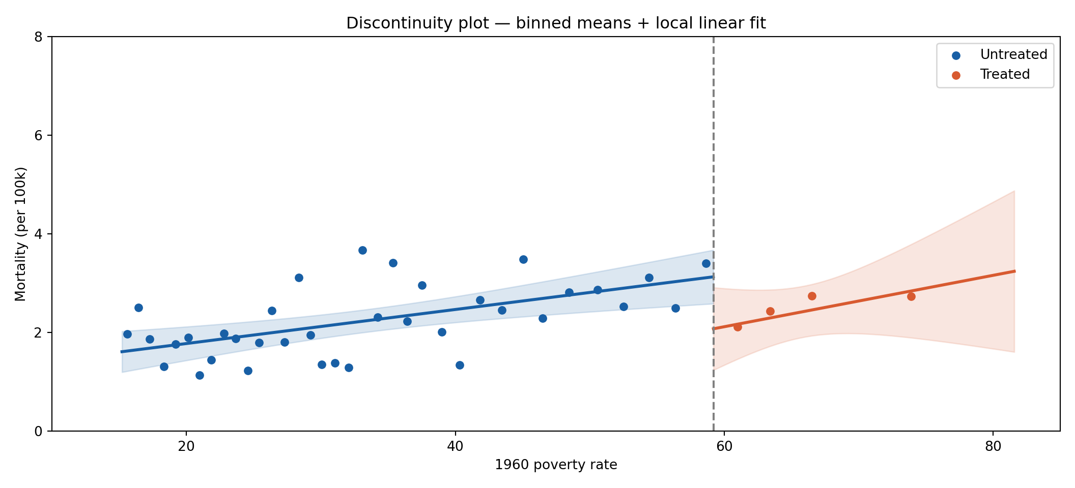
import pandas as pd, numpy as np, matplotlib.pyplot as plt, statsmodels.api as smhs = pd.read_csv("../data/rdd-headstart.csv"); C0 =59.1984q = np.quantile(hs.povrate60, np.linspace(0, 1, 41))hs["bin"] = pd.cut(hs.povrate60, np.unique(q), include_lowest=True)b = hs.groupby("bin", observed=True)[["povrate60", "mortHS"]].mean()fig, ax = plt.subplots(figsize=(11, 5))below = b.povrate60 < C0ax.scatter(b.povrate60[below], b.mortHS[below], color="#185FA5", s=28, label="Untreated")ax.scatter(b.povrate60[~below], b.mortHS[~below], color="#D85A30", s=28, label="Treated")for sub, col in [(hs[hs.povrate60 < C0], "#185FA5"), (hs[hs.povrate60 >= C0], "#D85A30")]: X = sm.add_constant(sub.povrate60); m = sm.OLS(sub.mortHS, X).fit() xs = np.linspace(sub.povrate60.min(), sub.povrate60.max(), 50) pr = m.get_prediction(sm.add_constant(xs)).summary_frame(alpha=0.05) # 95% CI band ax.plot(xs, pr["mean"], color=col, lw=2.2) ax.fill_between(xs, pr["mean_ci_lower"], pr["mean_ci_upper"], color=col, alpha=0.15)ax.axvline(C0, ls="--", color="grey")ax.set_xlim(10, 85); ax.set_ylim(0, 8)
(10.0, 85.0)
(0.0, 8.0)
Code
ax.set_xticks(range(20, 81, 20)); ax.set_yticks(range(0, 9, 2))ax.set_xlabel("1960 poverty rate"); ax.set_ylabel("Mortality (per 100k)")ax.set_title("Discontinuity plot — binned means + local linear fit"); ax.legend()plt.tight_layout(); plt.show()
Code
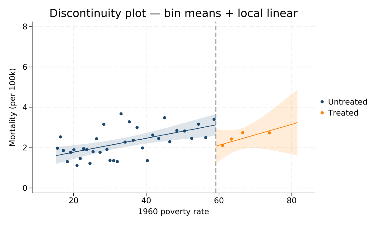
import delimited "../data/rdd-headstart.csv", case(preserve) clearscalar C0 = 59.1984gen treated = povrate60 >= C0* 40 equal-frequency bins (quantiles) of the running variable; plot binmeans +* linear fit WITH 95% CI band each side. Same axes as the R/Python tabs.egenbin = cut(povrate60), group(40)egen ybar = mean(mortHS), by(bin)egen xbar = mean(povrate60), by(bin)egentag = tag(bin)twoway (lfitci mortHS povrate60 if !treated, acolor(navy%15) alwidth(none) clcolor(navy)) /// (lfitci mortHS povrate60 if treated, acolor(orange%15) alwidth(none) clcolor(orange)) /// (scatter ybar xbar iftag & !treated, mcolor(navy)) /// (scatter ybar xbar iftag & treated, mcolor(orange)), ///xline(59.1984, lpattern(dash)) ///xscale(range(10 85)) xlabel(20(20)80) ///yscale(range(0 8)) ylabel(0(2)8) ///legend(order(5 "Untreated" 6 "Treated")) ///xtitle("1960 poverty rate") ytitle("Mortality (per 100k)") ///title("Discontinuity plot — bin means + local linear")graphexport"../plots/rdd_stata_rdplot.png", replacewidth(1600)
Warning
Binned means are a visual aid, not the estimate. They are a Nadaraya-Watson (rectangular, gridded) estimator — a poor one. Do not read the treatment effect off the dots; read it off the two local-linear fits at the cut-off. Hansen calls plotting only binned means “a bad habit”: always show the best nonparametric fit with confidence bands.
Bias grows with \(h^2\) and with curvature\(m''\) — a wider window “cuts the corner”.
Variance shrinks with \(nh\) (more effective observations) and with the density \(f(c)\) at the cut-off.
This bias-variance trade-off is the whole game in bandwidth choice.
The variance is estimated by summing the two boundary-regression sandwich variances. With \(Z_i = (1, X_i-c)'\), \(K_i = K((X_i-c)/h)\) and leave-one-out errors \(\tilde e_i\),
This is exactly the kernel-weighted sandwich we coded by hand (using raw residuals; rdrobust uses the leave-one-out variant).
Note
Honest inference. Bias does not vanish in finite samples. Two fixes: (i) use a common bandwidth on both sides (zeroes the first-order bias when \(m''\) is continuous); (ii) use a bandwidth smaller than MSE-optimal, trading variance for less bias. rdrobust instead bias-corrects the point estimate and widens the interval (robust CI).
Bandwidth Selection
Two Global Rules
Rule-of-thumb (Fan-Gijbels), with a level shift at (c): fit (m(x)=_0+_1 x++q x^q+{q+1}D) by OLS, form (’’), and
The constant (0.58) is for a variance-one kernel; use (1.00) for the rectangular and (1.42) for the unnormalised triangular kernel.
Cross-validation: pick (h) minimising the sum of squared leave-one-out prediction errors. Plot the CV criterion — if flat, bandwidths are hard to rank.
Advice (Hansen §21.6): compute the ROT for (q=2,3,4); the CV-minimiser is often near-infinite, so lean smaller than AMSE-optimal to reduce bias. For Head Start this gives (h).
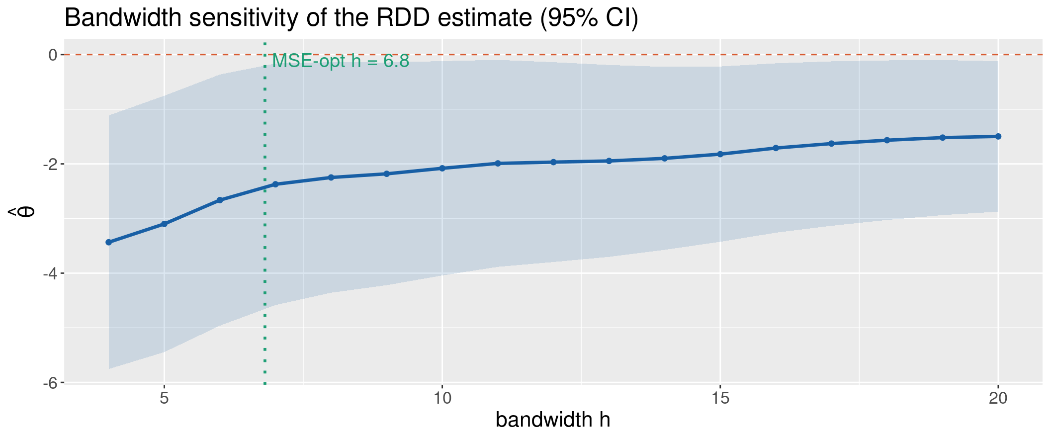
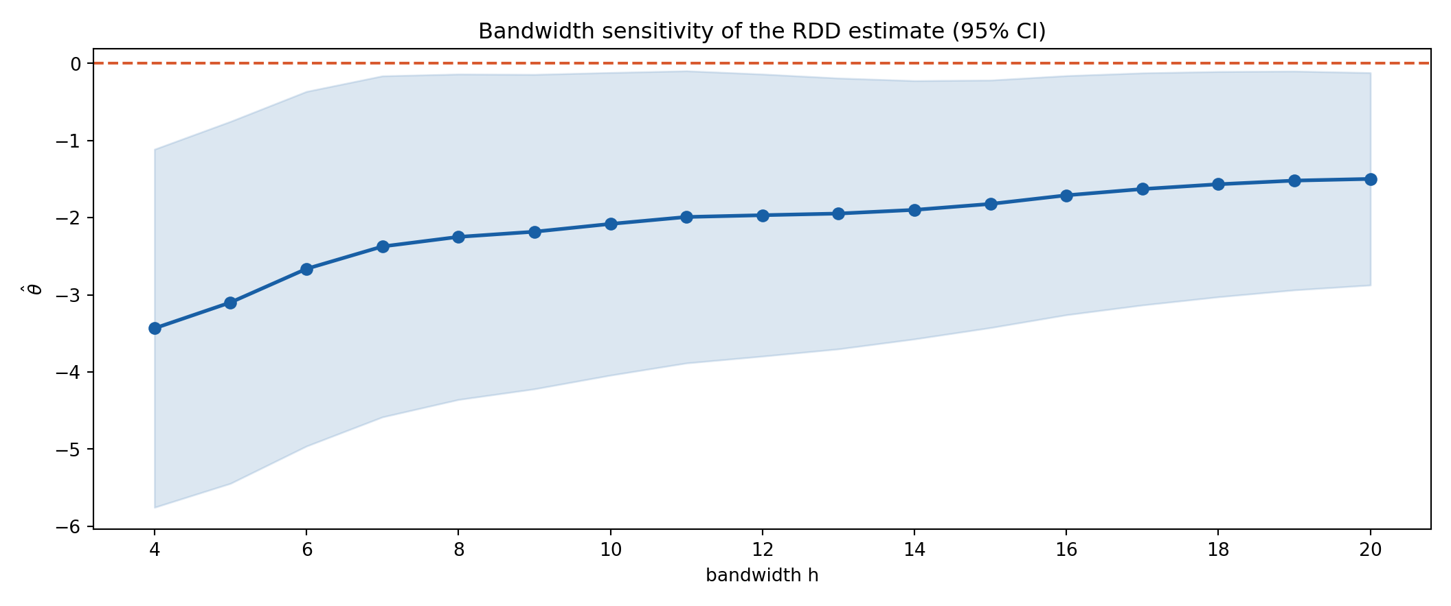
library(rdrobust)# Data-driven MSE-optimal bandwidth (Calonico-Cattaneo-Titiunik / Imbens-Kalyanaraman)bw <-rdbwselect(hs_df$mortHS, hs_df$povrate60, c = C0, bwselect ="mserd")summary(bw) # h (main) and b (bias) bandwidths# Sensitivity: theta across a grid of bandwidths (our hand-coded LL)hs <-seq(4, 20, by =1)sens <-t(sapply(hs, function(h) rd_ll(hs_df$mortHS, hs_df$povrate60, C0, h)))
Code
import pandas as pd, numpy as np, matplotlib.pyplot as plt, statsmodels.api as smhs = pd.read_csv("../data/rdd-headstart.csv"); C0 =59.1984def rd_ll(y, x, c, h): xx = x - c; D = (x >= c).astype(float); k = np.maximum(0, 1- np.abs(xx)/h) use = k >0; Z = np.column_stack([np.ones_like(xx), xx, D, xx*D])[use] f = sm.WLS(y[use], Z, weights=k[use]).fit(cov_type="HC1")return f.params[2], f.bse[2]hgrid = np.arange(4, 21)res = np.array([rd_ll(hs.mortHS.values, hs.povrate60.values, C0, h) for h in hgrid])th, se = res[:, 0], res[:, 1]plt.figure(figsize=(11, 4.6))plt.fill_between(hgrid, th -1.96*se, th +1.96*se, color="#185FA5", alpha=0.15)plt.plot(hgrid, th, "-o", color="#185FA5", lw=2)plt.axhline(0, ls="--", color="#D85A30")plt.xlabel("bandwidth h"); plt.ylabel(r"$\hat\theta$")plt.title("Bandwidth sensitivity of the RDD estimate (95% CI)")plt.tight_layout(); plt.show()
Code
import delimited "../data/rdd-headstart.csv", case(preserve) clearscalar C0 = 59.1984gen x = povrate60 - C0gen D = povrate60 >= C0gen xD = x*D* theta across bandwidths (rectangular windowfor a transparent, package-free sweep)foreachhof numlist 4 6 8 10 12 16 20 {quietlyregress mortHS x D xD ifabs(x)<=`h', vce(robust)dias txt "h = " %2.0f `h'" theta = "as res %7.3f _b[D] ///as txt " se = "as res %6.3f _se[D] as txt " n = "as res e(N)}
Tip
What the sweep shows. The estimate is negative and stable across \(h\): from about \(-2.7\) at \(h=6\) to \(-1.8\) at \(h=15\), straightening out (less curvature, more bias, narrower bands) as \(h\) grows. The MSE-optimal \(h \approx 6.8\) sits in the middle. Robustness to \(h\) — not to polynomial order — is the check that matters.
Boundary Bias & Robust Inference
Robust bias-corrected inference (CCT 2014)
Two steps beyond the conventional interval:
1. Bias-correct the point estimate. Estimate the leading bias (B,h^2) with a higher-order (pilot) local polynomial and subtract it: (_{} = - B,h^2).
2. Inflate the variance. The bias estimate (B) is itself noisy, so the CI must widen to account for that extra uncertainty — otherwise you undercover again.
The result is a CI centred on (_{}) whose width reflects both sampling and bias-estimation error. This is what rdrobust reports as Robust (as opposed to Conventional), and it attains nominal coverage even at the MSE-optimal bandwidth.
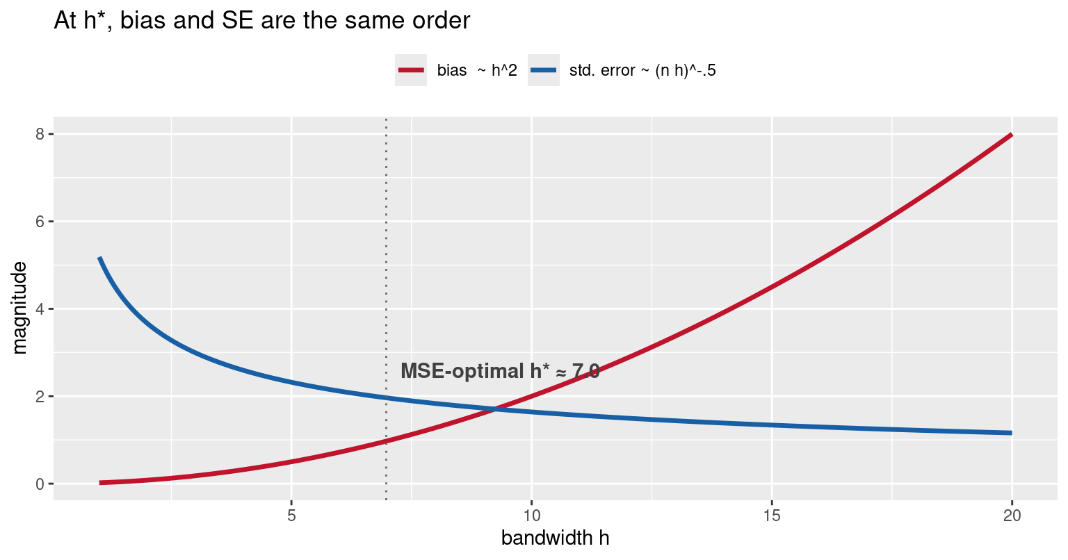
Big \(h\) → small variance but large bias (you borrow from far-away, curved regions).
Small \(h\) → small bias but large variance (few points near \(c\)).
The MSE-optimal\(h^\star \propto n^{-1/5}\)balances them — so at \(h^\star\) the bias is the same order as the SE.
Warning
Consequence. A conventional CI \(\hat\theta \pm 1.96\,\widehat{\text{SE}}\) is centred on a biased point, and the bias is not negligible relative to its width — so it undercovers (true coverage below \(95\%\)). Undersmoothing (shrinking \(h\) by hand) hides the bias but throws away precision.
Code
# Schematic: how bias (~ h^2) and SE (~ 1/sqrt(n h)) trade off with bandwidth.# Their sum of squares (MSE) is minimized at h*, where bias and SE are the# SAME ORDER — which is exactly why a conventional CI undercovers there.h <-seq(1, 20, length.out =300)n <-2783bias <-0.020* h^2# boundary smoothing biasse <-273.6/sqrt(n * h) # sampling SEmse <- bias^2+ se^2hopt <- h[which.min(mse)]df <-data.frame(h, bias, se)ggplot(df, aes(h)) +geom_line(aes(y = bias, colour ="bias ~ h^2"), linewidth =1.2) +geom_line(aes(y = se, colour ="std. error ~ (n h)^-.5"), linewidth =1.2) +geom_vline(xintercept = hopt, linetype ="dotted", colour ="grey40") +annotate("text", x = hopt +0.3, y =2.6, hjust =0,label =sprintf("MSE-optimal h* ≈ %.1f", hopt)) +scale_colour_manual(values =c("bias ~ h^2"="#C0132C","std. error ~ (n h)^-.5"="#185FA5")) +labs(x ="bandwidth h", y ="magnitude", colour =NULL,title ="At h*, bias and SE are the same order")
The red bias curve rises with \(h\); the blue SE curve falls. They cross near \(h^\star\) — precisely the regime where the conventional CI’s neglected bias bites. rdrobust’s Robust column fixes this (button above).
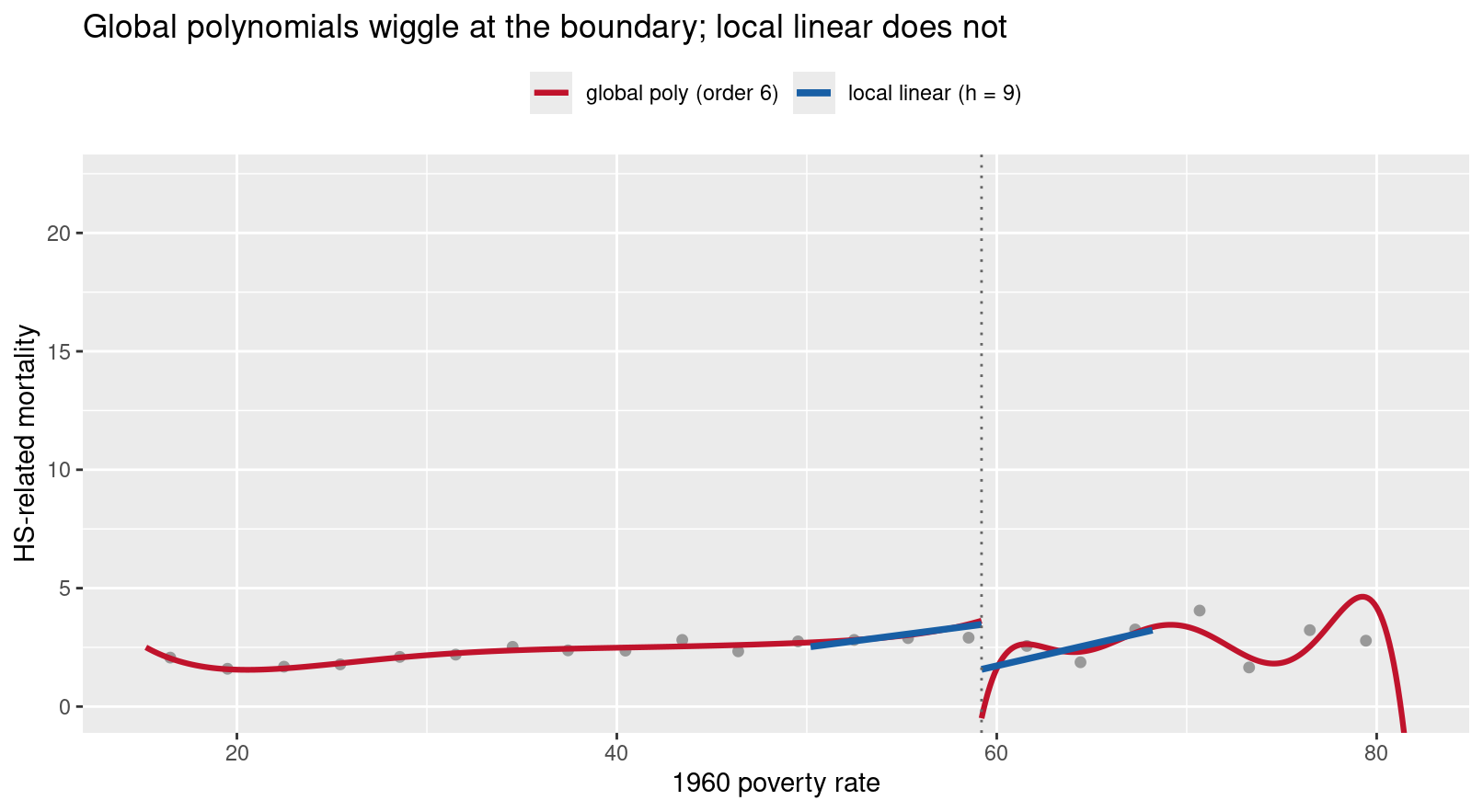
# Global high-order polynomial (order 6, fit each side) vs local linear (h = 9).# High-order global fits chase far-away points and wiggle at the boundary,# manufacturing a spurious jump at c. Local linear stays put. (Gelman & Imbens.)hs <-read.csv("../data/rdd-headstart.csv"); C0 <-59.1984L <-subset(hs, povrate60 < C0); R <-subset(hs, povrate60 >= C0)gL <-lm(mortHS ~poly(povrate60, 6), data = L) # global order 6, leftgR <-lm(mortHS ~poly(povrate60, 6), data = R) # global order 6, righthh <-9lL <-lm(mortHS ~ povrate60, data =subset(L, povrate60 > C0 - hh)) # local linearlR <-lm(mortHS ~ povrate60, data =subset(R, povrate60 < C0 + hh))gridL <-data.frame(povrate60 =seq(min(L$povrate60), C0, length =200))gridR <-data.frame(povrate60 =seq(C0, max(R$povrate60), length =200))# ... predict gL/gR (global) and lL/lR (local) on the grids, then plot with# binned means as a visual reference.
The global order-6 fit (red) swings wildly near the ends of the support and at the cut-off — its value at \(c\) is driven by data far away. The local linear fit (blue) uses only points within \(h=9\) of \(c\), so its boundary value is the one we trust.
Warning
Gelman & Imbens (2019): do not use high-order global polynomials in RDD. They:
assign large weights to observations far from \(c\), which is exactly where identification does not come from;
produce estimates that are highly sensitive to the polynomial order (order 4 vs 5 vs 6 can flip the sign of the “jump”);
deliver CIs with poor coverage.
The RDD estimand is a boundary object — use local low-order polynomials (linear or quadratic) with a principled bandwidth.
Report robustness to the bandwidth, not to ever-higher polynomial orders.
Power depends not on the total sample but on the effective sample inside the bandwidth — often a small fraction of the data. Two boundary points must each be pinned down from one side only, so RDD needs far more observations than a randomized experiment to reach the same power.
That is why an RDD can be significant yet underpowered: a wide robust CI signals that, ex ante, the design had only a modest chance of detecting a plausible effect. Reporting power/MDE alongside the estimate is honest practice.
Two questions, asked before (design) or after (interpretation) the study:
Power — given the design (bandwidth, variance, effective \(N\)), what is the probability of rejecting \(H_0:\bar\theta=0\) when the true effect is \(\tau\)? → rdpower.
Sample size — how many observations near \(c\) are needed for a target power (usually \(0.8\)) at effect \(\tau\)? → rdsampsi.
library(rdpower)hs <-read.csv("../data/rdd-headstart.csv")hs <- hs[complete.cases(hs[, c("povrate60","mortHS")]), ]Z <-cbind(hs$mortHS, hs$povrate60) # outcome, running variablerdpower(data = Z, cutoff =59.1984, tau =-2) # power to detect tau = -2rdsampsi(data = Z, cutoff =59.1984, tau =-2) # N needed for 0.8 power
For 80% power at tau = -2: need ~906 (left) + 364 (right) effective obs;
the study currently has 234 + 180 — i.e. it is underpowered for this effect.
Code
import pandas as pd, warningswarnings.filterwarnings("ignore")from rdpower import rdpowerhs = pd.read_csv("../data/rdd-headstart.csv").dropna(subset=["povrate60","mortHS"])Z = hs[["mortHS","povrate60"]] # outcome, running variablerdpower(data=Z, cutoff=59.1984, tau=-2, plot=False) # power to detect tau = -2
Number of obs  =  2783
BW type        =  mserd
Kernel type    =  Triangular
VCE method     =  NN
Derivative     =  0
HA:       tau  =  -2


Cutoff c = 59.198           Left of c      Right of c
Number of obs                   2489             294
Eff. # of obs                    234             180
BW loc. poly.                   6.81            6.81
Order loc. poly.                   1               1
Sampling BW                     6.81            6.81
New sample                       234             180


====================================================================================================
Power against:                H0: tau =      0.2*tau =      0.5*tau =      0.8*tau =          tau =
                                    0           -0.4           -1.0           -1.6             -2
----------------------------------------------------------------------------------------------------
Robust bias-corrected            0.05           0.06          0.113          0.215          0.309
====================================================================================================
{'power_rbc': 0.3094766696167214, 'se_rbc': np.float64(1.3682259049252694), 'sampsi_r': np.int64(180), 'sampsi_l': np.int64(234), 'samph_r': np.float64(6.810478803394809), 'samph_l': np.float64(6.810478803394809), 'N_r': np.int64(294), 'N_l': np.int64(2489), 'Nh_l': np.int64(234), 'Nh_r': np.int64(180), 'tau': -2, 'bias_r': np.float64(0.005453098569993304), 'bias_l': np.float64(-0.0025591091267016296), 'Vr_rb': np.float64(4921.377317379724), 'Vl_rb': np.float64(30560.49015605024), 'alpha': 0.05}
Code
import delimited "../data/rdd-headstart.csv", case(preserve) clearrdpower mortHS povrate60, c(59.1984) tau(-2) // power to detect tau = -2rdsampsi mortHS povrate60, c(59.1984) tau(-2) // N needed for 0.8 power
power at \(\tau=-2\)
\(N\) for \(0.8\) power
R
\(0.309\)
\(\approx 906 + 364\)
Python
\(0.309\)
\(\approx 906 + 364\)
Stata
\(0.309\)
\(\approx 906 + 364\)
At the MSE-optimal bandwidth, the Head Start design has only 31% power to detect an effect of \(\tau=-2\) — it is underpowered for that magnitude.
To reach \(80\%\) power you would need roughly \(906\) (left) + \(364\) (right) effective observations, versus the \(234 + 180\) actually available.
This reconciles the wide robust CI with the significant point estimate: the study got a clear signal, but had it not, we should not have been surprised. Report power, not just the \(p\)-value.
Covariates \(Z\) are not needed for identification (Theorem 21.1 already gives \(\bar\theta\)). They can, however, reduce the equation error and sharpen precision. Assume a partially-linear form:
The conditional ATE is still \(\bar\theta = m(c{+}) - m(c{-})\). The Robinson (1988) semiparametric estimator:
LL-regress \(Y\) on \(X\) → fitted \(\hat m_i\); LL-regress each \(Z_k\) on \(X\) → \(\hat g_{ki}\).
OLS of \((Y_i - \hat m_i)\) on \((Z_{ki} - \hat g_{ki})\) → \(\hat\beta\).
Form \(\hat e_i = Y_i - Z_i'\hat\beta\); LL-regress \(\hat e_i\) on \(X\) → \(\hat m(x)\), \(\hat{\bar\theta}\).
A convenient practical version just adds \(Z\) to the windowed regression.
Code
library(sandwich); library(lmtest)sub <-abs(hs_df$povrate60 - C0) <=8dd <-transform(hs_df, x = povrate60 - C0, D =as.numeric(povrate60 >= C0))base <-lm(mortHS ~ x + D + x:D, data = dd, subset = sub)covs <-lm(mortHS ~ x + D + x:D + pctblack + pcturban, data = dd, subset = sub)cb <-coeftest(base, vcov =vcovHC(base, "HC1"))cc <-coeftest(covs, vcov =vcovHC(covs, "HC1"))tab <-data.frame(``=c("theta (D)", "s(theta)", "% Black", "% Urban"),Baseline =c(sprintf("%.2f", cb["D",1]), sprintf("(%.2f)", cb["D",2]), "", ""),Covariates =c(sprintf("%.2f", cc["D",1]), sprintf("(%.2f)", cc["D",2]),sprintf("%.4f (%.4f)", cc["pctblack",1], cc["pctblack",2]),sprintf("%.4f (%.4f)", cc["pcturban",1], cc["pcturban",2])),check.names =FALSE)kbl(tab, align =c("l","r","r"),caption ="RDD estimate of Head Start on child mortality (h = 8, n = 482)") %>%kable_styling(font_size =20, full_width =TRUE, bootstrap_options =c("striped","hover")) %>%row_spec(1, bold =TRUE, color = col_accent)
RDD estimate of Head Start on child mortality (h = 8, n = 482)
Baseline
Covariates
theta (D)
-2.20
-2.17
s(theta)
(1.06)
(1.06)
% Black
0.0129 (0.0120)
% Urban
-0.0087 (0.0121)
The treatment effect is essentially unchanged (\(-2.20 \to -2.17\)) — as theory predicts. The covariate signs (% Black \(>0\), % Urban \(<0\)) are consistent with these acting as income proxies (Hansen Table 21.1).
Covariate Adjustment — When It’s “Free”
Only adjust for covariates that do NOT jump at c
The estimand is preserved only if each covariate (Z) is itself continuous at the cut-off (Calonico, Cattaneo, Farrell & Titiunik 2019).
If a covariate jumps at (c), then it is partly an outcome of treatment. Adjusting for it absorbs part of the effect and biases () — the classic “bad control” problem.
Rule: use only predetermined covariates (measured before treatment), and check their continuity at (c) exactly as you check the outcome. A covariate that fails the balance test should not be used for adjustment.
and the only thing that can change is the variance:
Covariates that predict \(Y\) near \(c\) soak up residual noise → smaller SE.
Covariates uncorrelated with \(Y\) near \(c\) → essentially no gain (and a few lost degrees of freedom).
Note
Precision is not guaranteed. On Head Start, % Black and % Urban barely correlate with mortality among near-cut-off counties, so the SE falls by well under \(1\%\). The estimand-invariance, by contrast, is exact — that is the real reason to feel safe adding predetermined covariates.
Code
hs <-read.csv("../data/rdd-headstart.csv")hs <- hs[complete.cases(hs[, c("povrate60","mortHS","pctblack","pcturban")]), ]# covs = predetermined 1960 covariates, continuous at the cut-offo0 <-rdrobust(hs$mortHS, hs$povrate60, c =59.1984)o1 <-rdrobust(hs$mortHS, hs$povrate60, c =59.1984,covs =cbind(hs$pctblack, hs$pcturban))
no covs : tau = -2.409 se = 1.206
+ covs : tau = -2.381 se = 1.198
estimand shift = +0.028 SE change = -0.7%
Code
import pandas as pd, warningswarnings.filterwarnings("ignore")from rdrobust import rdrobusths = pd.read_csv("../data/rdd-headstart.csv").dropna( subset=["povrate60","mortHS","pctblack","pcturban"])o0 = rdrobust(y=hs.mortHS, x=hs.povrate60, c=59.1984)o1 = rdrobust(y=hs.mortHS, x=hs.povrate60, c=59.1984, covs=hs[["pctblack","pcturban"]])print(f"no covs : tau = {float(o0.coef.iloc[0,0]):+.3f} se = {float(o0.se.iloc[0,0]):.3f}")
no covs : tau = -2.409 se = 1.206
Code
print(f"+ covs : tau = {float(o1.coef.iloc[0,0]):+.3f} se = {float(o1.se.iloc[0,0]):.3f}")
Identical across languages; the estimate moves by only \(0.03\) — estimand invariance in action.
The SE change is negligible here — covariates don’t predict mortality near the cut-off. Adjust for validity insurance and possible precision, never expecting a free lunch.
The cut-off effect can differ across subgroups\(G\). Estimate all group effects in one kernel-weighted regression by fully interacting the local-linear terms with \(G\) (here \(G\in\{0,1\}\)):
\[Y = \alpha + \beta x + \theta D + \gamma xD \; + \; G\big(\alpha_1 + \beta_1 x + \theta_1 D + \gamma_1 xD\big) + \varepsilon,\]
\(\theta\) = cut-off effect for group \(G=0\); \(\theta + \theta_1\) = effect for \(G=1\).
\(\theta_1\) is the heterogeneity: a \(t\)-test on \(\theta_1\) asks whether the RDD effect differs across groups.
Equivalent to running separate RDDs per group — which is exactly what rdrobust does below, group by group.
Warning
Local samples get small fast. Splitting the data shrinks the effective sample within \(h\) on each side, inflating every subgroup SE. Treat subgroup RDD effects as exploratory unless each cell is well-populated.
Code
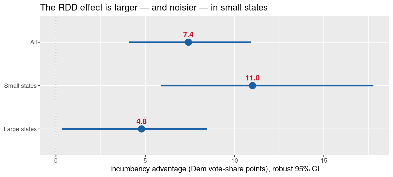
sen <-read.csv("../data/rdd-senate.csv")# incumbency advantage overall, then split states by 1960 population (median)fit <-function(d) { o <-rdrobust(d$vote, d$margin, c =0)c(est = o$coef[1], lo = o$ci[3, 1], hi = o$ci[3, 2]) }med <-median(sen$population, na.rm =TRUE)res <-rbind(All =fit(sen),`Small states`=fit(subset(sen, population < med)),`Large states`=fit(subset(sen, population >= med)))# forest plot of the three robust CIs ...
The incumbency advantage is about twice as large in small states (\(\approx 11\) pts) as in large ones (\(\approx 5\) pts), but each subgroup interval is wider than the pooled one — the price of splitting the local sample.
Heterogeneity is a statement about effect modification at the cut-off, still fully local in \(X\).
Report it with the same rigour as the main effect: MSE-optimal bandwidth per group, robust CIs.
A significant \(\theta_1\) (or non-overlapping CIs) is suggestive, not proof — pre-register subgroups to avoid fishing.
Modern extension: continuously-varying heterogeneity via covariate interactions (Calonico–Cattaneo–Farrell–Palomba–Titiunik).
library(rdrobust)# MSE-optimal bandwidth + robust bias-corrected inference (CCT 2014), triangular kernel.out <-rdrobust(hs_df$mortHS, hs_df$povrate60, c = C0) # kernel="tri", bwselect="mserd" by defaultsummary(out)# Read: 'Conventional' = point estimate at MSE-opt h; 'Robust' = bias-corrected CI (use this).
rdrobust — Head Start (triangular kernel, MSE-optimal bandwidth)
main bandwidth h = 6.810 bias bandwidth b = 10.725
effective N: left = 234 right = 180
Conventional: tau = -2.409 se = 1.206
Robust (bias-corrected): p = 0.042 95% CI = [-5.462, -0.099]
Code
import pandas as pdfrom rdrobust import rdrobust # pip install rdrobust — same API as Rhs = pd.read_csv("../data/rdd-headstart.csv"); C0 =59.1984out = rdrobust(y=hs.mortHS, x=hs.povrate60, c=C0) # triangular kernel, MSE-optimal bandwidthprint(f"MSE-optimal h = {float(out.bws.iloc[0, 0]):.3f} bias b = {float(out.bws.iloc[1, 0]):.3f}")
MSE-optimal h = 6.810 bias b = 10.725
Code
print(f"Conventional: tau = {float(out.coef.iloc[0]):.3f} se = {float(out.se.iloc[0]):.3f}")
Conventional: tau = -2.409 se = 1.206
Code
print(f"Robust (bias-corrected): p = {float(out.pv.iloc[2]):.3f} "f"95% CI = [{float(out.ci.iloc[2, 0]):.3f}, {float(out.ci.iloc[2, 1]):.3f}]")
Robust (bias-corrected): p = 0.042 95% CI = [-5.462, -0.099]
Code
* ssc install rdrobust // one-time; then the same command as R:import delimited "../data/rdd-headstart.csv", case(preserve) clearrdrobust mortHS povrate60, c(59.1984) // triangular kernel, MSE-optimal bandwidth
rdrobust() key arguments:
Argument
Default
What it controls
c
0
Cut-off on the running variable
p
1
Local polynomial order (1 = local linear)
kernel
"triangular"
Boundary-optimal weighting
bwselect
"mserd"
MSE-optimal common bandwidth (also cerrd for coverage)
h, b
data-driven
Main and bias bandwidths (set manually to override)
vce
"nn"
Nearest-neighbour variance; "hc1",… also available
covs
none
Add covariates (Robinson-style)
On Head Start: MSE-optimal \(h \approx 6.81\), \(\hat\tau_{\text{conv}} = -2.41\), and the robust bias-corrected 95% CI is \([-5.46,\,-0.10]\) (\(p = 0.042\)) — significant, and consistent with our hand-coded \(-2.2\) to \(-2.3\).
Tip
Report the robust CI, not the conventional one, when the bandwidth is data-driven: bias correction plus the wider interval is what makes the inference honest (Calonico, Cattaneo & Titiunik 2014).
RDD’s credibility rests on continuity + no manipulation. These generate testable implications:
Threat
What breaks
Falsification test
Manipulation / sorting
Density of \(X\) jumps at \(c\)
McCrary density test
Confounded jump
Covariates jump at \(c\)
Covariate balance / continuity
It’s not the cut-off
Effect appears at fake \(c\)
Placebo cut-offs
It’s not the treatment
Effect on unaffected outcome
Placebo outcomes
Tip
A validity checklist before you believe an RDD:
Plot the raw data + local-linear fit with CI bands.
Run the density test — no bunching at \(c\).
Check pre-determined covariates are continuous at \(c\).
Run placebo cut-offs (fake thresholds) — no effect.
Run placebo outcomes (things treatment can’t affect) — no effect.
Show the estimate is stable across bandwidths.
Manipulation (Density) Test
The continuity assumption fails if units sort across the cut-off. Then the density\(f(x)\) of the running variable is discontinuous at \(c\) (bunching). McCrary (2008) tests \(H_0: f(c{+}) = f(c{-})\).
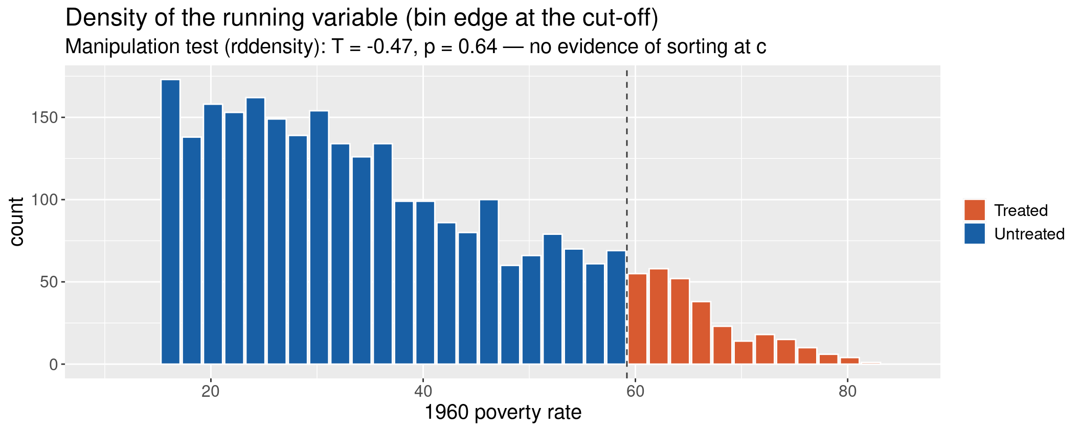
# Formal test: rddensity::rddensity(hs_df$povrate60, c = C0) (if installed)# Package-free visual: fine histogram with a bin edge exactly at the cut-off.library(rddensity) # optionaldt <-rddensity(hs_df$povrate60, c = C0)summary(dt) # T stat & p-value for a density jump
Code
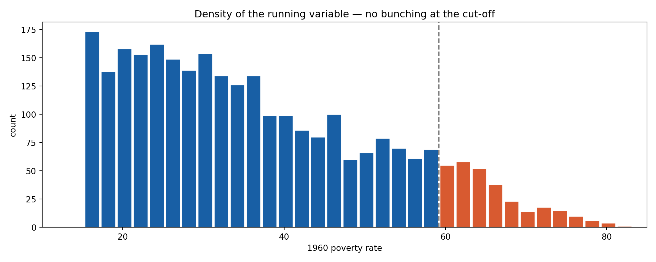
import pandas as pd, numpy as np, matplotlib.pyplot as plths = pd.read_csv("../data/rdd-headstart.csv"); C0 =59.1984lo =int(np.floor((hs.povrate60.min() - C0) /2)); hi =int(np.ceil((hs.povrate60.max() - C0) /2))brks = C0 +2.0* np.arange(lo, hi +1) # bins 2 wide, an edge exactly at the cut-offcnt, edges = np.histogram(hs.povrate60, bins=brks)mid =0.5* (edges[:-1] + edges[1:])col = np.where(mid >= C0, "#D85A30", "#185FA5")plt.figure(figsize=(11, 4.4))plt.bar(mid, cnt, width=1.8, color=col, edgecolor="white")plt.axvline(C0, ls="--", color="grey")plt.xlim(10, 85); plt.xticks(range(20, 81, 20))
(10.0, 85.0)
([<matplotlib.axis.XTick object at 0x7f8a9ad96c80>, <matplotlib.axis.XTick object at 0x7f8a9ad75660>, <matplotlib.axis.XTick object at 0x7f8a9adf6aa0>, <matplotlib.axis.XTick object at 0x7f8a9adf5660>], [Text(20, 0, '20'), Text(40, 0, '40'), Text(60, 0, '60'), Text(80, 0, '80')])
Code
plt.xlabel("1960 poverty rate"); plt.ylabel("count")plt.title("Density of the running variable — no bunching at the cut-off")plt.tight_layout(); plt.show()
Code
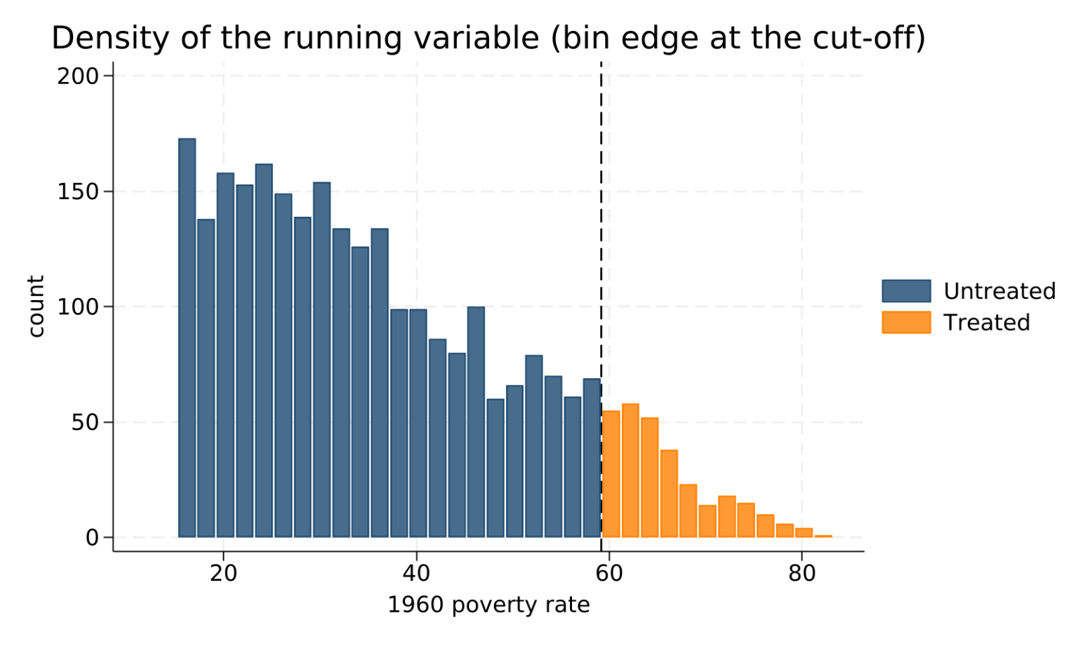
import delimited "../data/rdd-headstart.csv", case(preserve) clear* Bins 2 wide with an edge EXACTLY at the cut-off (asin R/Python), coloured by* side, counts. start = cut-off minus a whole number ofbin widths.quietlysummarize povrate60localstart = 59.1984 - 2 * ceil((59.1984 - r(min)) / 2)gen binmid = `start' + 2 * floor((povrate60 - `start') / 2) + 1 // bin centregen side = povrate60 >= 59.1984preservecollapse (count) cnt = povrate60 (mean) side, by(binmid)twoway (bar cnt binmid if side == 0, barwidth(1.8) color(navy)) /// (bar cnt binmid if side == 1, barwidth(1.8) color(orange)), ///xline(59.1984, lpattern(dash)) ///xscale(range(10 85)) xlabel(20(20)80) ///legend(order(1 "Untreated" 2 "Treated")) ///xtitle("1960 poverty rate") ytitle("count") ///title("Density of the running variable (bin edge at the cut-off)")graphexport"../plots/rdd_stata_density.png", replacewidth(1600)restore* Formal manipulation test (Cattaneo, Jansson & Ma) — H0: density continuous at crddensity povrate60, c(59.1984)
Note
Head Start passes. The rddensity test gives \(T = -0.47\), \(p = 0.64\) (R and Stata agree) — no evidence of a density jump. That is expected: the running variable is a 1960 census poverty rate, fixed by a federal agency in 1965, so counties could not manipulate it to get onto the treated side. Where the running variable is manipulable (self-reported income, re-sittable test scores), this test is essential.
# Placebo CUT-OFFS: re-estimate at fake thresholds where no policy switches.for (cc inc(45, 50, 55, 65, 70))print(rd_ll(hs_df$mortHS, hs_df$povrate60, cc, 8))# Placebo OUTCOMES: things Head Start should NOT move.rd_ll(hs_df$mort_injury, hs_df$povrate60, C0, 8) # child injuries (unrelated cause)rd_ll(hs_df$mort_adult, hs_df$povrate60, C0, 8) # adults 25+ (wrong age group)rd_ll(hs_df$mort_preHS, hs_df$povrate60, C0, 8) # 1959-64 (before the programme)
Falsification: placebo cut-offs (top) and placebo outcomes (bottom), h = 8
Check
theta
se
t
Placebo cut-offs (should be ~0)
cut-off = 45
-1.596
1.762
-0.91
cut-off = 50
0.942
1.068
0.88
cut-off = 55
0.279
1.006
0.28
cut-off = 65
0.631
0.968
0.65
cut-off = 70
-0.208
2.049
-0.10
Placebo outcomes (should be ~0)
TRUE outcome (HS mortality)
-2.249
1.076
-2.09
placebo: child injuries
0.183
3.484
0.05
placebo: adults 25+
2.038
6.274
0.32
placebo: pre-1965
-3.433
1.857
-1.85
Code
import pandas as pd, numpy as np, statsmodels.api as smhs = pd.read_csv("../data/rdd-headstart.csv"); C0 =59.1984def rd_ll(y, x, c, h=8): xx = x - c; D = (x >= c).astype(float); k = np.maximum(0, 1- np.abs(xx)/h); use = k >0 Z = np.column_stack([np.ones_like(xx), xx, D, xx*D])[use] f = sm.WLS(y[use], Z, weights=k[use]).fit(cov_type="HC1")return f.params[2], f.bse[2]print("Placebo cut-offs (theta, se):")
Placebo cut-offs (theta, se):
Code
for cc in [45, 50, 55, 65, 70]: th, se = rd_ll(hs.mortHS.values, hs.povrate60.values, cc);print(f" c={cc}: {th:7.3f} ({se:.3f})")
print("\nPlacebo outcomes at true cut-off (theta, se):")
Placebo outcomes at true cut-off (theta, se):
Code
for v, lab in [("mortHS","TRUE"),("mort_injury","injuries"),("mort_adult","adults25+"),("mort_preHS","pre-1965")]: th, se = rd_ll(hs[v].values, hs.povrate60.values, C0);print(f" {lab:9s}: {th:7.3f} ({se:.3f})")
import delimited "../data/rdd-headstart.csv", case(preserve) clearprogram rdll // theta at cutoff `2' for outcome `1', h=8gen x = povrate60 - `2'gen D = povrate60 >= `2'gen xD = x*Dgenk = max(0, 1 - abs(x)/8)quietlyregress`1' x D xD [aweight=k] ifk>0, vce(robust)dias txt " theta = "as res %7.3f _b[D] as txt " (se "as res %5.3f _se[D] as txt ")"drop x D xD kenddias txt "Placebo cut-offs (true outcome):"foreachccof numlist 45 50 55 65 70 { dias txt "c=`cc'" _c; rdll mortHS `cc' }dias txt "Placebo outcomes at true cut-off 59.1984:"foreachyin mortHS mort_injury mort_adult mort_preHS { dias txt "`y'" _c; rdll `y' 59.1984 }
Placebo cut-offs (45, 50, 55, 65, 70): all \(|t| < 1.1\) — no discontinuity at fake thresholds. The effect is specific to the real policy cut-off. ✓
Placebo outcomes: child injuries (\(-0.16\), se \(3.4\)) and adult mortality (\(+2.1\), se \(5.9\)) show no effect — Head Start targets young children’s disease mortality, not injuries or adults. ✓
Pre-1965 mortality (\(-3.7\), se \(1.9\)) is only borderline — a mild caveat worth probing (Exercise), but far weaker than the post-period effect.
Tip
Placebo outcomes are the most persuasive falsification: they show the discontinuity appears only where the mechanism predicts it should.
Local Randomization View
Two ways to justify RDD
Continuity (the default): smooth potential-outcome regressions, large-sample local-polynomial inference, MSE-optimal bandwidth. Approximation improves as the sample grows.
Local randomization (Cattaneo–Frandsen–Titiunik 2015): inside a narrow window ([c-w,,c+w]) treatment is as if randomly assigned, so the window behaves like a tiny randomized experiment. Inference is finite-sample exact (Fisher randomization), needing no smoothness or large-n asymptotics.
Local randomization is especially attractive with few observations or a discrete running variable — settings where continuity-based asymptotics are shaky. Its cost: the window must be small enough for the “as-good-as-random” assumption to hold, which you defend with covariate balance.
Pick a window \(W = [c-w,\, c+w]\) so narrow that, within it, which side of \(c\) a unit lands on is as good as a coin flip. Then:
Window selection — grow \(w\) until predetermined covariates stop being balanced; the largest balanced window is \(W\) (rdwinselect).
Randomization inference — under Fisher’s sharp null \(H_0: Y_{1i}=Y_{0i}\ \forall i\), permute the treatment labels within \(W\) and recompute a statistic \(T\) (e.g. difference in means). The exact\(p\)-value is \[p = \frac{1}{|\Omega|}\sum_{\pi\in\Omega} \mathbb{1}\{|T(\pi)| \ge |T_{\text{obs}}|\}.\]
No bandwidth-bias correction, no asymptotics — valid in finite samples.
Code
library(rdlocrand)hs <-read.csv("../data/rdd-headstart.csv")hs <- hs[complete.cases(hs[, c("povrate60","mortHS")]), ]R <- hs$povrate60 -59.1984# running variable centred at the cut-off# Fisher randomization inference in a fixed window (balance-selected: +/- 2)out <-rdrandinf(hs$mortHS, R, wl =-2, wr =2, reps =5000, seed =14159)
window = [-2, 2]
N in window = 124
diff in means = -2.5206
randomization p = 0.0140
Code
import pandas as pd, numpy as np# No rdlocrand port — the permutation test is three lines of numpy.hs = pd.read_csv("../data/rdd-headstart.csv").dropna(subset=["povrate60","mortHS"])R = hs.povrate60.values -59.1984Y = hs.mortHS.valuesm = np.abs(R) <=2# fixed window +/- 2Yw, Dw = Y[m], (R[m] >=0).astype(int)obs = Yw[Dw ==1].mean() - Yw[Dw ==0].mean()rng, reps = np.random.default_rng(14159), 5000count =0for _ inrange(reps): p = rng.permutation(Dw) # reassign treatment within the windowifabs(Yw[p ==1].mean() - Yw[p ==0].mean()) >=abs(obs): count +=1print(f"window = [-2, 2]")
window = [-2, 2]
Code
print(f"N in window = {m.sum()}")
N in window = 124
Code
print(f"diff in means = {obs:.4f}")
diff in means = -2.5206
Code
print(f"randomization p = {(count +1) / (reps +1):.4f}")
The difference in means (\(-2.52\)) and window count (\(N=124\)) are identical across languages (deterministic).
The randomization \(p\)-value is simulation-based, so implementations agree up to Monte-Carlo error (Stata reports a finite-sample \(0.008\) and a large-sample \(0.021\); R/Python’s permutation gives \(0.014\)). All say the same thing: significant at the \(5\%\) level.
Reassuringly, the local-randomization estimate (\(-2.52\)) matches the continuity-based rdrobust estimate (\(-2.41\)) — two very different justifications, one conclusion.
Discrete Running Variables
Clustering on the score is not a cure
A once-common fix (Lee & Card 2008) was to cluster the standard errors on the running-variable value, treating the gap between the true regression and the local fit as random specification error.
Kolesár & Rothe (2018) show this can badly under- or over-cover: the clustered SE has no guarantee, because the “specification error” is a fixed function, not noise. They recommend honest confidence intervals instead — intervals built to have correct coverage uniformly over all regression functions with a bounded second derivative (you supply the smoothness bound).
Bottom line: with a discrete score, reach for honest CIs (RDHonest) or the local-randomization framework — not a reflexive cluster option.
Standard RDD asymptotics assume \(X\) is continuous with positive density at \(c\), so the bandwidth can shrink to zero with more data. Many real running variables are discrete: age in years, integer test scores, birth weights, calendar dates.
With finitely many mass points, there is a smallest gap around \(c\) — you cannot let \(h\to 0\). More data means more observations per point, not points closer to \(c\).
So a residual approximation (specification) error never vanishes, and the usual local-polynomial standard errors are too small ⇒ conventional CIs undercover.
The fewer the distinct values near \(c\), the worse the continuity-based approximation.
Note
Our Head Start score (povrate60) is effectively continuous (many decimals), so this issue does not bite here — but it is central whenever the score is coarse.
Cluster by the score (Lee & Card 2008). Model the fit error as random and cluster SEs on the value of \(X\). Historically standard — but see the caveat popup: it carries no coverage guarantee.
Honest CIs (Kolesár & Rothe 2018). Assume only a bound on the second derivative of \(m(\cdot)\) and construct intervals with guaranteed coverage uniformly over that class. Implemented in RDHonest. This is the modern recommendation.
Local randomization. With very few mass points, drop asymptotics entirely and use finite-sample Fisher inference in a window (previous slide) — naturally suited to a discrete score.
Report the number of distinct values of \(X\) near \(c\) — it tells the audience how discrete the design really is.
In rdrobust, the masspoints option ("adjust" / "check") detects repeated values and adjusts the bandwidth and variance accordingly.
Prefer honest CIs or local randomization when the score is coarse; treat naive local-polynomial CIs as optimistic.
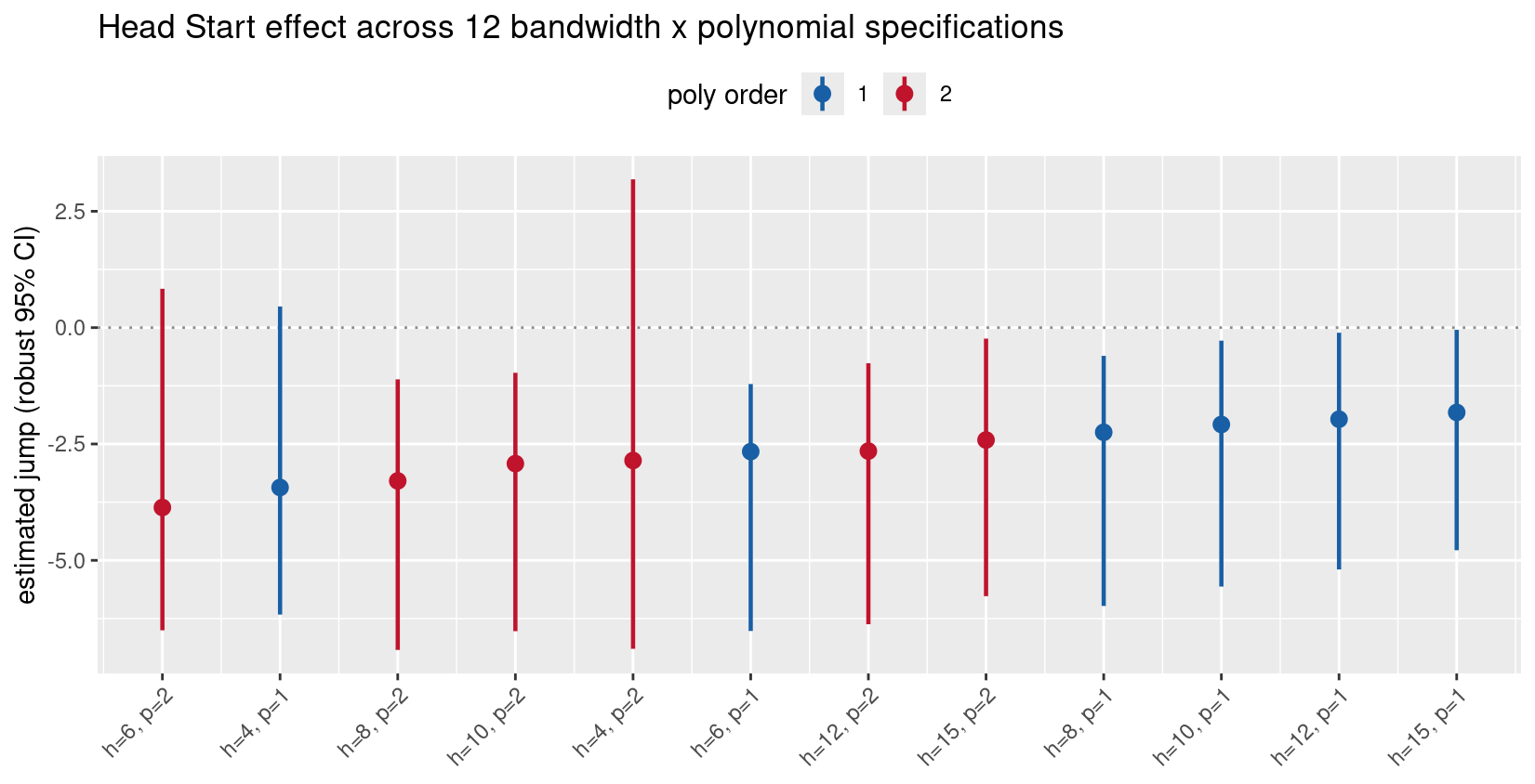
hs <-read.csv("../data/rdd-headstart.csv")# Re-estimate the jump across a grid of bandwidth x polynomial order.# A credible RDD result is stable across reasonable specifications.grid <-expand.grid(h =c(4, 6, 8, 10, 12, 15), p =c(1, 2))est <-data.frame()for (i inseq_len(nrow(grid))) { o <-rdrobust(hs$mortHS, hs$povrate60, c =59.1984,h = grid$h[i], p = grid$p[i]) est <-rbind(est, data.frame(h = grid$h[i], p = grid$p[i],tau = o$coef[1], lo = o$ci[3, 1], hi = o$ci[3, 2]))}# plot tau with robust CI, ordered by point estimate ...
Every one of the 12 specifications gives a negative estimate, and most exclude zero — the finding that Head Start reduced child mortality is not an artefact of one bandwidth or polynomial choice.
A specification curve plots the estimate (with CI) under many defensible analytic choices at once — here bandwidth \(\times\) polynomial order.
Look for: the sign holding, the bulk of CIs on one side of zero, and no single knob flipping the conclusion.
Red flags: the estimate swinging across the zero line as \(h\) or \(p\) changes, or significance resting on one lucky cell.
It complements — does not replace — reporting your pre-specified primary specification (MSE-optimal \(h\), local linear) up front.
Warning
A specification curve is a transparency device, not a licence to cherry-pick. Decide the grid before looking at the estimates, and show the whole curve.
Part VI — Fuzzy RDD
Fuzzy RDD — Theory
A Weak Instrument in Disguise
The fuzzy estimator divides by (p(c+)-p(c-)), the jump in the treatment probability. If that jump is small, the denominator is near zero and () is a weak-IV statistic: large variance, finite-sample bias toward the OLS estimate, and unreliable normal-approximation CIs.
Always plot and test the first stage — the discontinuity in (p(x)=(D=1X=x)). It is the reduced form of the IV design; identification rests on its magnitude, not just its sign.
A Head-Start-style take-up jump of (0.40) (denominator ()) is a comfortably strong first stage.
In many designs the cut-off changes the probability of treatment, not treatment itself — imperfect compliance. Define
\[p(x) = \Pr(D = 1 \mid X = x),\qquad \text{FRD applies when } p(c{+}) \ne p(c{-}).\]
For Head Start, the real take-up was 80% above vs 43% below the cut-off — a textbook fuzzy design (we treated it as sharp intent-to-treat earlier).
Theorem 21.2 (Hahn, Todd & Van der Klaauw 2001). If \(m_0, m_1\) are continuous at \(c\), \(p(x)\) is discontinuous at \(c\), and \(D\) is independent of \(\theta\) for \(X\) near \(c\), then \[\boxed{\;\bar\theta = \dfrac{m(c{+}) - m(c{-})}{p(c{+}) - p(c{-})}\;}\]
The conditional ATE is the ratio of two jumps: the jump in the outcome over the jump in the treatment probability.
is exactly a Wald / 2SLS estimator: regress \(Y\) on \(D\), instrumenting\(D\) with the assignment \(Z = \mathbb{1}\{X \ge c\}\), locally near \(c\) (controlling for the running variable). Numerator = reduced form; denominator = first stage. Sharp RDD is the special case \(p(c{+}) - p(c{-}) = 1\).
Fuzzy RDD is an instrumental-variables design at the cut-off, with instrument \(Z = \mathbb{1}\{X\ge c\}\). It rests on the standard IV triad, stated locally at \(c\):
Relevance (strong first stage).\(p(c{+}) \ne p(c{-})\) — the cut-off actually shifts treatment probability. A tiny jump ⇒ weak instrument (see popup).
Exclusion restriction. Crossing \(c\) affects \(Y\)only through\(D\) — no other channel switches at the threshold (this is the “no coincident treatments” condition wearing an IV hat).
Monotonicity (no defiers). Crossing \(c\) pushes everyone’s treatment the same direction: units are compliers or always-/never-takers, but nobody is treated because they fell below \(c\).
Under monotonicity the fuzzy estimand is not the full-population ATE but a Local Average Treatment Effect — the effect for compliers at the cut-off: the units whose treatment status is flipped by crossing \(c\). \[\bar\theta_{\text{FRD}} = \mathbb{E}\!\left[\,Y_1 - Y_0 \;\middle|\; \text{complier},\, X = c\,\right].\]
Always-takers and never-takers cancel from both jumps, so they contribute nothing to \(\bar\theta_{\text{FRD}}\) — the estimand is doubly local: local in \(X\) (at \(c\)) and local in the population (compliers only).
library(AER)fuzzy_df <-read.csv("../data/rdd-fuzzy.csv"); h <-20sub <-abs(fuzzy_df$X) <= h # window around c = 0# First stage: jump in treatment probability p(c+)-p(c-)fs <-lm(D ~ X + Z, data = fuzzy_df, subset = sub)# Reduced form: jump in the outcome m(c+)-m(c-)rf <-lm(Y ~ X + Z, data = fuzzy_df, subset = sub)cat(sprintf("first stage jump_D = %.3f | reduced form jump_Y = %.3f | Wald = %.3f\n",coef(fs)["Z"], coef(rf)["Z"], coef(rf)["Z"]/coef(fs)["Z"]))# 2SLS: Y on D, instrument D with Z, control for the running variable Xiv <-ivreg(Y ~ D + X | Z + X, data = fuzzy_df, subset = sub)coeftest(iv, vcov =vcovHC(iv, type ="HC1")) # coef on D = fuzzy RDD estimate
Fuzzy RDD — simulated data (true LATE = 3.0), window |X| <= 20
first stage: p(c+)-p(c-) = 0.421 (take-up 0.40 -> 0.80)
first stage jump_D = 0.421 | reduced form jump_Y = 1.230 | Wald = 2.922
Code
# 2SLS: dependent Y; exog [const, X]; endog D; instrument Ziv = IV2SLS(fz.Y, sm.add_constant(fz[["X"]]), fz[["D"]], fz[["Z"]]).fit(cov_type="robust")print(f"2SLS LATE = {iv.params['D']:.3f} se = {iv.std_errors['D']:.3f} n = {len(fz)}")
2SLS LATE = 2.922 se = 0.174 n = 1995
Code
import delimited "../data/rdd-fuzzy.csv", case(preserve) clear* First stage and reduced form (jumps at the cut-off c = 0)quietlyregress D X Z ifabs(X)<=20scalar jD = _b[Z]quietlyregress Y X Z ifabs(X)<=20scalar jY = _b[Z]dias txt "first stage jump_D = "as res %5.3f jD ///as txt " | reduced form jump_Y = "as res %5.3f jY ///as txt " | Wald = "as res %5.3f jY/jD* Fuzzy RDD via 2SLS: Y on D (instrumented by Z), controlling for Xivregress 2sls Y X (D = Z) ifabs(X)<=20, vce(robust)dias txt "2SLS LATE = "as res _b[D] as txt " se = "as res _se[D]
Quantity
Value
Meaning
First stage \(p(c{+})-p(c{-})\)
\(\approx 0.40\)
take-up jumps \(0.40 \to 0.80\) — strong
Reduced form \(m(c{+})-m(c{-})\)
\(\approx 1.17\)
ITT jump in the outcome
2SLS LATE
\(\approx 2.92\)
ratio ≈ recovers the true LATE of \(3.0\)
The point estimate is identical across R, Python and Stata (\(2.92\)); robust SEs agree to \(\approx 0.01\).
The Wald ratio scales up the intent-to-treat jump by the compliance rate: dividing \(1.17\) by \(0.40\) recovers the effect on compliers.
Sharp RDD is the limit where the first stage \(= 1\); there, reduced form \(=\) LATE.
Warning
Check the first stage first. A tiny denominator ⇒ weak-instrument problems (huge SEs, bias). Report \(p(c{+})-p(c{-})\) and its \(t\)-statistic alongside the LATE.
Many rules make the level of a benefit continuous but bend its slope at a threshold — think an unemployment-insurance formula that replaces a higher fraction of earnings below a cap, or a tax schedule that changes marginal rate at a bracket. Then the treatment effect shows up as a change in slope, not a jump.
The level\(m(x)\) is continuous at \(c\); its first derivative is not.
Identification (Card–Lee–Pei–Weber 2015): under smoothness of the potential-outcome derivatives, the slope change at \(c\) identifies the marginal effect of the policy variable.
Estimate with a local polynomial and read off the first derivative on each side:
rdrobust(..., deriv = 1) returns \(m'(c^{+}) - m'(c^{-})\) directly, with MSE-optimal bandwidth and robust bias-corrected inference.
Polynomial order. Use \(p \ge \text{deriv}\). For a piecewise-linear schedule (UI, tax brackets are literally piecewise linear) local linear (\(p=1\)) is exact; with genuine curvature raise to \(p=2\).
Cost. Derivative estimation inflates variance — expect wider CIs than a sharp level jump on the same sample.
Warning
A kink is not a jump. If you run a level RDD on kinked data you will (correctly) find no jump and wrongly conclude “no effect.” Match the estimator (deriv = 1) to the design.
kink <-read.csv("../data/rdd-kink.csv")# Benefit schedule bends at c = 0: level continuous, slope jumps 0.5 -> 2.0.# deriv = 1 estimates the slope change; p = 1 is exact for a piecewise-linear rule.out <-rdrobust(kink$Y, kink$X, c =0, deriv =1, p =1)summary(out)
print(f"MSE-optimal h = {float(out.bws.iloc[0,0]):.3f}")
MSE-optimal h = 0.310
Code
print(f"true kink = 1.500")
true kink = 1.500
Code
import delimited "../data/rdd-kink.csv", case(preserve) clearrdrobust y x, c(0) deriv(1) p(1) // deriv(1) = slope jump; p(1) local linear
All three languages return the same slope jump on the shared rdd-kink.csv:
Estimate
True
R
\(1.445\)
\(1.5\)
Python
\(1.445\)
\(1.5\)
Stata
\(1.445\)
\(1.5\)
The estimate sits close to the true kink of \(1.5\) and is highly significant (\(p \approx 10^{-8}\)).
Because the schedule is piecewise linear, local linear (\(p=1\)) recovers each slope exactly — deriv = 1 differences them.
Try deriv = 1, p = 2 on this data: the extra curvature term only adds variance here (no curvature to fit), so the CI widens — a concrete reminder to match \(p\) to the design.
Geographic RDD
A border switches many things at once
The identifying assumption is that only the treatment changes at the boundary. Real borders often coincide with other discontinuities — school-district quality, tax regimes, house prices, language, historical institutions.
If several policies jump at the same line, the estimate is a compound treatment effect, not the one you want (Keele & Titiunik 2015). Defend against it by checking covariate balance along the border and, where possible, comparing multiple border segments that share your treatment but differ in the confounders.
Also watch for sorting: people can move across a border to get the treatment (Tiebout sorting), violating no-manipulation in a way a one-dimensional density test may miss.
When treatment is assigned by which side of a border a unit sits on, the “running variable” is a geographic location\((\text{lat}, \text{lon})\) — a two-dimensional score, and the cut-off is an entire boundary curve, not a point.
Distance-to-border reduction. Collapse the 2-D score to a signed distance to the nearest boundary point and run a standard 1-D RDD on it. Simple, but throws away where along the border each unit is.
Boundary-point (local) approach. Estimate a separate effect at each point of the border and average — respects that the treatment contrast may vary along the boundary (Keele & Titiunik 2015).
Bandwidth is a distance band hugging the border; only units within that band enter.
Geographic designs face everything a 1-D RDD does, plus:
Compound treatments — many things change at a border (see popup); the estimate may bundle them.
Spatial sorting — households can relocate across the line to obtain treatment, a manipulation channel invisible to a naive density test.
Spatial correlation — nearby units are dependent; use spatially-robust / clustered SEs.
Sparse borders — few observations in the distance band ⇒ wide CIs.
Note
Software: rdrobust still does the 1-D estimation once you have the distance score; specialised spatial tooling (e.g. distance construction, border-point sampling) lives in GIS + the RD packages’ geographic vignettes. Reference: Keele & Titiunik (2015), Political Analysis.
Some policies use a different threshold for different groups — income limits that vary with family size, grade boundaries that differ by cohort. Each unit \(i\) faces its own cut-off \(c_i\).
Normalize and pool. Recentre every unit on its own cut-off, \(\tilde X_i = X_i - c_i\), and run one RDD at \(\tilde X = 0\). Efficient, but assumes the effect is common across cut-offs.
Cut-off-by-cut-off. Estimate a separate effect at each \(c_j\) and inspect heterogeneity — the pooled number can mask very different local effects (Cattaneo, Titiunik & Vazquez-Bare 2016).
Report both: the pooled estimate for power, the per-cut-off estimates for transparency.
Sometimes treatment needs two conditions — pass a math score and a reading score; qualify on incomeandassets. The boundary is now a frontier in score-space.
Frontier RDD. Estimate the treatment effect along the qualification frontier, which can differ at each point (e.g. the effect for those marginal on math vs marginal on reading).
Distance-to-frontier reduction. As with geographic RDD, collapse the multi-score problem to a signed distance to the nearest frontier point and run a 1-D RDD.
Each unit contributes at the frontier point closest to it; effects can be heterogeneous across the frontier.
Tip
The unifying trick behind geographic, multi-cutoff and multi-score designs is the same: reduce a complicated assignment boundary to a one-dimensional signed distance, then apply the standard local-polynomial machinery — while remembering the effect may vary along that boundary. Reference: Cattaneo, Titiunik & Vazquez-Bare (2016), Stata Journal.
A Second Sharp RDD — Senate Incumbency
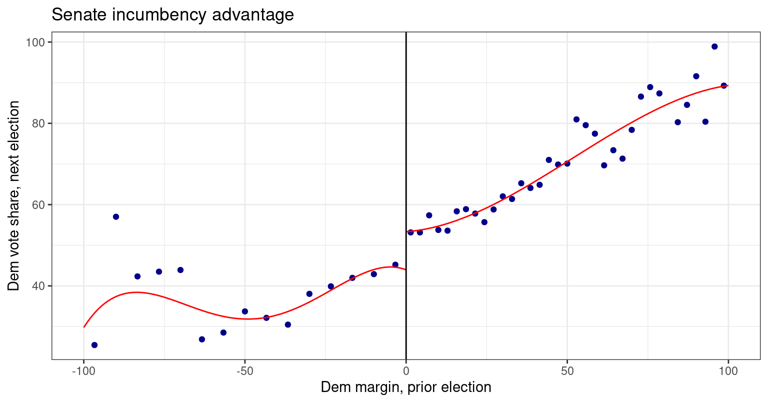
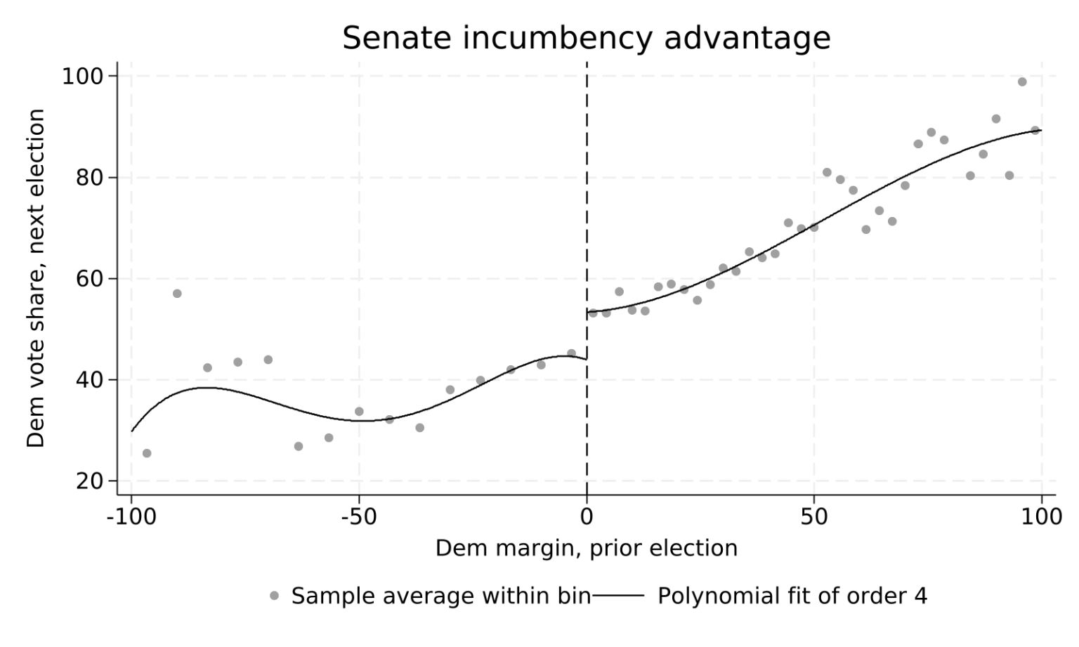
The whole workflow, in a different policy domain. Cattaneo–Frandsen–Titiunik US Senate data: does winning a Senate seat (Democratic margin \(\ge 0\) in the prior election) raise the party’s vote share in the next election? Running variable margin, outcome vote, cut-off \(0\).
sen <-read.csv("../data/rdd-senate.csv")rdplot(sen$vote, sen$margin, c =0, # binned means + polynomial fitx.label ="Dem margin, prior election",y.label ="Dem vote share, next election",title ="Senate incumbency advantage")rdrobust(sen$vote, sen$margin, c =0) # MSE-optimal, robust bias-corrected
incumbency advantage = +7.414 vote-share points
robust 95% CI = [4.09, 10.92] p = 1.6e-05
MSE-optimal h = 17.75 Nh = 360 / 323
Code
import pandas as pd, warningswarnings.filterwarnings("ignore")import matplotlib.pyplot as pltfrom rdrobust import rdrobust, rdplotsen = pd.read_csv("../data/rdd-senate.csv")rdplot(y=sen.vote, x=sen.margin, c=0, x_label="Dem margin, prior election", y_label="Dem vote share, next election", title="Senate incumbency advantage")
Call: rdplot
Number of Observations:                  1297
Kernel:                               Uniform
Polynomial Order Est. (p):                  4

                                Left      Right
------------------------------------------------
Number of Observations           595        702
Number of Effective Obs          595        702
Bandwidth poly. fit (h)        100.0      100.0
Number of bins scale               1          1
Bins Selected                     15         35
Average Bin Length             6.667      2.857
Median Bin Length              6.667      2.857
IMSE-optimal bins                8.0        9.0
Mimicking Variance bins         15.0       35.0

Relative to IMSE-optimal:
Implied scale                  1.875      3.889
WIMSE variance weight          0.132      0.017
WIMSE bias weight              0.868      0.983
Code
plt.show()
Code
o = rdrobust(y=sen.vote, x=sen.margin, c=0)print(f"incumbency advantage = {float(o.coef.iloc[0,0]):+.3f} vote-share points")
incumbency advantage = +7.414 vote-share points
Code
print(f"MSE-optimal h = {float(o.bws.iloc[0,0]):.2f}")
Winning nearly-tied elections raises the party’s next vote share by about 7.4 points — a large, precisely-estimated incumbency advantage (\(p < 10^{-4}\)).
Identical across R, Python and Stata on the shared rdd-senate.csv, exactly as for Head Start.
Same recipe, new domain: rdplot for the picture, rdrobust for the MSE-optimal robust estimate.
flowchart TD
    d1{"Threshold rule<br/>on an observable X?"}
    d3{"Density of X<br/>continuous at c?"}
    d4{"Running variable<br/>continuous or discrete?"}
    d2{"Compliance at c?"}
    dk{"Level jump<br/>or slope change?"}
    b1["Choose bandwidth h<br/>(MSE-opt) + poly order p<br/>(local linear); add<br/>predetermined covs"]
    o1["Sharp RDD<br/>LL: m(c+) - m(c-)"]
    o2["Fuzzy RDD<br/>Wald / 2SLS"]
    ok["Kink RDD<br/>rdrobust deriv=1"]
    lr["Local randomization<br/>rdrandinf in window W"]
    v1["Validity: density test,<br/>placebo cut-offs/outcomes,<br/>covariate balance, spec curve"]
    done(["Report robust CI"])
    s1["RDD not applicable<br/>(use IV / DiD / matching)"]
    s2["Manipulation!<br/>design invalid"]

    d1 -->|Yes| d3
    d1 -->|No| s1
    d3 -->|No| s2
    d3 -->|Yes| d4
    d4 -->|Continuous| d2
    d4 -->|Discrete / few mass points| lr
    d2 -->|Perfect| dk
    d2 -->|Imperfect| o2
    dk -->|Level| o1
    dk -->|Slope| ok
    o1 --> b1
    o2 --> b1
    ok --> b1
    b1 --> v1
    lr --> v1
    v1 --> done

    classDef decision fill:#dbeafe,stroke:#185FA5,color:#0c2461,font-weight:bold
    classDef process  fill:#e0f2fe,stroke:#185FA5,color:#1e40af,font-weight:bold
    classDef outcome  fill:#d1fae5,stroke:#1D9E75,color:#064e3b,font-weight:bold
    classDef sideout  fill:#fef3c7,stroke:#D85A30,color:#92400e,font-weight:bold

    class d1,d2,d3,d4,dk decision
    class b1 process
    class o1,o2,ok,lr,done outcome
    class s1,s2 sideout
Mistake
Consequence
Fix
High-order global polynomial
Spurious jumps, unstable CI
Local linear + small \(h\)
vcovHC on a weighted lm
SE badly understated
Hand sandwich / rdrobust
Reading effect off binned dots
Wrong magnitude
Read the LL fit at \(c\)
Ignoring the first stage (fuzzy)
Weak-IV bias
Report \(p(c{+})-p(c{-})\)
No manipulation test
Undetected sorting
McCrary density test
Level estimator on kink data
“No effect” — misses the slope jump
rdrobust deriv(1)
Adjusting for a covariate that jumps at \(c\)
Bad control — biases \(\hat{\bar\theta}\)
Use only predetermined, balanced covs
Extrapolating \(\bar\theta\) away from \(c\)
Wrong population
Keep it local
Tip
RDD buys credibility with a local parameter. Guard continuity (density + placebos), keep the window small, and always report robustness to the bandwidth.
Exercises — Estimation
Bandwidth sensitivity. Re-estimate the Head Start sharp RDD (local linear, triangular) for \(h = 4, 6, 8, 12, 20\). Tabulate \(\hat{\bar\theta}\) and its SE. At which \(h\) does the estimate lose significance, and why?
Kernel choice. Compare the triangular-kernel estimate to the rectangular (simple OLS) estimate at \(h = 8\). Explain the small difference in terms of efficiency at the boundary.
Reproduce Hansen eq. (21.5). Using rdd-headstart.csv, run the windowed OLS \(Y = \beta_0 + \beta_1 X + \beta_3(X-c)D + \theta D + e\) on \(|X-c|\le 8\). Confirm \(\hat\theta = -2.20\) (se \(1.06\), \(n = 482\)) in all three languages.
Covariates. Add pctblack and pcturban. Does \(\hat{\bar\theta}\) change? Explain why Theorem 21.1 predicts this, and what the covariates buy you.
rdrobust. Run rdrobust(mortHS, povrate60, c = 59.1984). Report the MSE-optimal bandwidth and the robust (bias-corrected) 95% CI. Contrast conventional vs robust inference.
Fuzzy vs sharp. In rdd-fuzzy.csv, estimate the sharp (reduced-form) jump in \(Y\) and the fuzzy 2SLS LATE. Verify LATE \(=\) (jump in \(Y\)) / (jump in \(D\)). Which one answers “the effect of treatment”?
Exercises — Validity
Placebo cut-offs. Estimate the Head Start effect at fake cut-offs \(c \in \{45, 50, 55, 65, 70\}\). Should any be significant? Interpret a spurious rejection if you find one.
Placebo outcomes. Estimate the discontinuity in mort_injury (child injuries) and mort_adult (adults 25+). Why are these good falsification tests for the Head Start mechanism?
Pre-programme check. Estimate the discontinuity in mort_preHS (1959-64, before Head Start). It is borderline. Discuss what a pre-period effect would imply for the design, and one way to probe it further.
Manipulation. Build a fine histogram of povrate60 with a bin edge exactly at \(59.1984\). Is there bunching? Why is manipulation a priori implausible for this running variable?
First-stage strength (fuzzy). In rdd-fuzzy.csv, report \(p(c{+})-p(c{-})\) and its \(t\)-statistic. Shrink the true take-up jump toward \(0\) (re-simulate) and watch the 2SLS SE explode — the weak-instrument problem.
Bias vs variance. Explain, using the bias and variance formulas, why shrinking \(h\) below the MSE-optimal value can produce “more honest” (if less precise) inference.
Second dataset — Senate. Using rdd-senate.csv, reproduce the incumbency advantage (\(\approx +7.4\) points) with rdrobust in R, Python and Stata. Then run rddensity (margin manipulation) and a covariate-balance check on demvoteshlag1 — does the design pass?
Local randomization. On Head Start, use rdwinselect (with pctblack, pcturban) to pick a balanced window, then rdrandinf for the finite-sample \(p\)-value. Compare it to the continuity-based rdrobust result and explain why they need different assumptions.
Specification curve. Re-estimate the Head Start jump across the \(6\times 2\) grid of bandwidth \(\times\) polynomial order. Plot the sorted estimates with robust CIs. Does the sign of the effect ever flip?