Every named model in Part 4 is a restriction of it. The deck’s argument is that choosing which restriction to impose is an empirical question (Part 3), that estimating it is a numerical one (Part 5), and that interpreting it is where most applied papers go wrong (Part 6).
One deliberate departure from the standard order: the tests come before the models, because the Anselin decision rule is how the model gets chosen. Each test still has its own theory slide and code slide.
Companion decks own neighbouring ground and are not repeated here.
Networks and Trade Analysis builds the same object this deck calls \(\mathbf{W}\) — an adjacency matrix — and asks what its structure looks like: centrality, communities, degree distributions. This deck asks what that structure does to an estimator. Part 1 shows the identical matrix under both readings.
Panel TWFE and Panel OLS/FE/RE own clustered standard errors and the Pesaran CD test, which detects cross-sectional dependence without offering a remedy. Part 8 is the remedy, and includes the Conley standard errors that no other deck in this series can currently produce.
That deck asks what does this network look like? This deck asks once my observations can influence each other, which of my cross-section habits still work — and what does \(\beta\) even mean?
import numpy as np # arrays, the Jacobianimport pandas as pd # data framesimport geopandas as gpd # geometry and centroidsimport libpysal # weights objects, built from the shared tripletsfrom libpysal.weights import W # the native weight objectimport esda # Moran's I, Geary's C, local Moran (LISA)import spreg # ML_Lag, ML_Error, GM_Lag, GM_Error_Hetimport matplotlib.pyplot as plt # all figures
* All native to Stata SE since Stata 15 - no installation needed:spmatrix spfrommata // build W from the shared triplet filespset // attach the spatial data structurespmatrix normalize // row-standardisationspregress // SAR / SEM / SDM by ML or GS2SLSspivregress // spatial IVspxtregress // spatial panels with fixed or random effectsestat moran // Moran's I on residualsestat impact // direct / indirect / total impacts
All three languages are genuinely strong here — this is the most balanced deck of the recent additions. R’s spdep/spatialreg are the oldest and most complete, PySAL is the reference implementation of most of the tests, and Stata’s sp* suite is native and excellent.
Data & Provenance
255 European NUTS-2 regions — the EU plus candidate countries (Turkey, Serbia, North Macedonia). Everything public and free to download.
File
Content
Source
spat-nuts.csv
GDP per head (PPS), average growth 2000–2024, population, tertiary-education share
Queen-contiguity weights, sparse triplet form (i, j, w)
derived from the geometry
spat-W-knn.csv
5-nearest-neighbour weights, same form
derived from the geometry
spat-sim.csv
Known-truth SAR sample: \(\rho = 0.5\), \(\beta = (1, -0.8)\), set by us
simulated, seed 14159
The weight matrix is data, and it is built once. R’s listw, PySAL’s W and Stata’s spmatrix are three native objects that cannot read each other. If each tab built its own \(\mathbf{W}\) from geometry, the three tabs would silently estimate three different models. So both matrices ship as sparse triplets, and each tab constructs its native object from that same file in a few visible lines. All three languages agree exactly: 1275 non-zeros for the \(k\)-nearest-neighbour matrix, 1088 for contiguity.
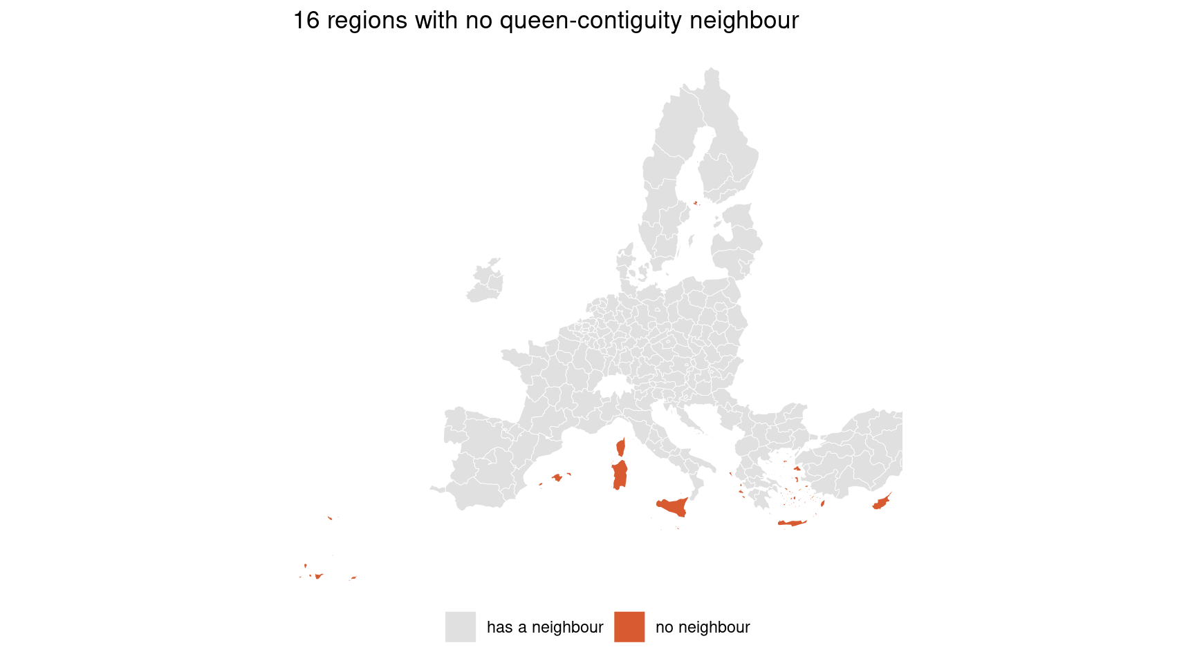
Islands are kept, not dropped.16 of the 255 regions — Malta, Cyprus, the Canaries, Åland, Corsica, Sicily, Sardinia, the Azores, Madeira and the Aegean islands — have no queen-contiguity neighbour at all, so their row of \(\mathbf{W}\) sums to 0 rather than 1. Silently removing them would change the sample; instead the \(k\)-nearest-neighbour matrix is the primary specification and contiguity the robustness check — the reverse of the textbook order, and Part 2 explains why.
A regional development grant is paid to Attiki. Two years later, output per head has risen in Sterea Elláda next door, which received nothing.
Three explanations, and they demand different models:
Workers commute across the boundary, so the grant’s effect spills over
Both regions were on the same trajectory anyway — a common shock the grant had nothing to do with
Whatever drives growth in one place drives it in the other, and it is simply missing from the regression
Only the first is a treatment effect on the neighbour. The other two are confounds that will masquerade as one.
The uncomfortable part: the standard toolkit cannot tell them apart, because it was built on an assumption that has already been violated by the time the question is asked.
Once observations can influence each other, the row of your data is no longer the unit of analysis. Almost every habit from cross-section econometrics needs re-deriving — including what \(\beta\) means.
SUTVA, stated and then violated
Every causal deck in this series leans on the Stable Unit Treatment Value Assumption. It has two parts, and spatial data breaks the first:
\[Y_i(\mathbf{d}) = Y_i(d_i) \qquad \text{for all treatment vectors } \mathbf{d}\]
Region \(i\)’s outcome depends on its own treatment \(d_i\) and on nothing anybody else received. Write out what that forbids:
That is exactly the spillover we just described. If the grant to Attiki raises output in Sterea Elláda, this derivative is not zero, and the potential-outcome notation \(Y_i(1), Y_i(0)\) is no longer even well defined — region \(i\) has as many potential outcomes as there are treatment configurations of everyone else.
What breaks, precisely, when SUTVA fails
With \(N\) units and binary treatment, the potential-outcome function of unit \(i\) is a map from \(\{0,1\}^N\) to the reals. SUTVA collapses those \(2^N\) arguments to \(2\). Drop it and three things go at once.
The estimand stops existing. “The” average treatment effect \(E[Y_i(1) - Y_i(0)]\) presumes a single control state. Under interference there are many: untreated with no treated neighbours, untreated with three treated neighbours, and so on. You must say which one you mean.
The control group is contaminated. Untreated neighbours of treated units absorb part of the treatment. Differencing against them subtracts the spillover from the direct effect, biasing the estimate toward zero — the classic understatement in evaluations of place-based policy.
Randomisation does not save you. Random assignment makes \(d_i\) independent of potential outcomes; it says nothing about \(d_j\) for a neighbour \(j\). A perfectly executed RCT with interference still returns a biased estimate of the direct effect.
The spatial-econometric response is to stop pretending the derivative is zero and to parameterise it, through a weight matrix \(\mathbf{W}\) that declares who is a neighbour and a coefficient that measures how much a neighbour matters. That is the whole apparatus of this deck.
The modern causal-inference response — partial interference, exposure mappings, spillover-robust estimators — keeps the design-based framing and restricts how interference may travel instead. Part 8 returns to it.
Tobler’s law is not yet econometrics
Everything is related to everything else, but near things are more related than distant things. — Waldo Tobler (1970)
True, and almost useless as stated. It tells you dependence exists; it does not tell you what to estimate. Three things have to be added before there is a model:
Who counts as near? Tobler does not say. You must choose, and the choice is \(\mathbf{W}\) — Part 2
How much more related? That is a parameter to estimate, not a fact to assert — Parts 4 and 5
Related how? Through the outcome, through the regressors, or through the error — and these are different models with different consequences
The last point is the one that gets skipped. “There is spatial autocorrelation in my residuals” is a diagnosis with at least three distinct treatments, and picking the wrong one is worse than picking none.
Why “add a distance control” does not fix it
A common reflex is to put latitude, longitude, or distance-to-capital on the right-hand side and declare the geography controlled for. It is not the same thing.
A smooth trend surface in coordinates — say \(\alpha_1 \text{lon}_i + \alpha_2 \text{lat}_i\) — models spatial heterogeneity: the mean varies over space. It says nothing about spatial interaction: that \(i\)’s outcome responds to \(j\)’s outcome. Two regions with the same coordinate-implied mean can still be linked, and adding coordinates leaves that link entirely in the error term.
Concretely, suppose the truth is \(\mathbf{y} = \rho \mathbf{W} \mathbf{y} + \mathbf{X}\beta + \varepsilon\). Adding a trend surface to \(\mathbf{X}\) does not remove \(\rho \mathbf{W} \mathbf{y}\); it is still an omitted, endogenous regressor. The Moran test on the residuals will still reject, and \(\hat\beta\) will still be biased — usually by slightly less, which is the dangerous part, because the diagnostic looks improved.
Region fixed effects have the same limitation in reverse: they absorb heterogeneity completely and interaction not at all.
The distinction is exactly the one on the next slide, and it is why the deck spends Part 3 on testing before Part 4 on models.
Knowledge spills over, firms follow suppliers, tax rates respond to neighbouring tax rates. The dependence is economic behaviour, and it is usually what we want to measure.
Consequence: \(\mathbf{W}\mathbf{y}\) is correlated with \(\varepsilon\) by construction, so OLS is inconsistent. This is a simultaneity, not a nuisance.
The return to education is not the same in Bavaria as in Calabria. Nothing spills over; the parameters simply differ, and pooling them manufactures autocorrelated residuals out of nothing.
Consequence: a global model is misspecified, and it will look spatially autocorrelated even though no region influences any other. The remedy is fixed effects, interactions or geographically weighted regression — not a spatial lag.
Climate, soil, a shared institution, a regional shock nobody measured. No behavioural spillover — just an unobservable that does not respect borders.
Consequence: \(\hat{\boldsymbol{\beta}}\) stays unbiased, but it is inefficient and the standard errors are wrong. This is the spatial analogue of serial correlation.
The three produce the same symptom — a significant Moran’s I on OLS residuals — and demand opposite responses.
Source
\(\hat{\boldsymbol{\beta}}\)
Inference
Remedy
Interaction
biased
invalid
model \(\mathbf{W}\mathbf{y}\)
Heterogeneity
biased if pooled
invalid
let parameters vary
Nuisance
unbiased
invalid
model the error, or robust SEs
Reading a rejected Moran test as automatic evidence for a spatial lag is the single most common error in applied work. The next slide prices it.
What OLS does when you ignore it
Two simulations on the 255 real European regions and their \(k\)-nearest-neighbour matrix. Truth is \(\beta = 1\) in both. The regressor is itself spatially clustered, as every regional covariate is.
Interaction ignored — \(\hat\beta \approx 1.42\) against a truth of 1, and the nominal 95% interval covers the true value in essentially none of 500 samples
Nuisance ignored — \(\hat\beta \approx 1.00\), unbiased, but the reported standard error is only about 70% of the true sampling variability, so coverage falls to ≈85%
Code
set.seed(14159)a <-read.csv("../data/spat-nuts.csv")wk <-read.csv("../data/spat-W-knn.csv")N <-nrow(a)# the shared triplet file becomes a dense WW <-matrix(0, N, N)W[cbind(wk$i, wk$j)] <- wk$w# these inverses are fixed across replications, so build them onceAi <-solve(diag(N) -0.5* W) # spatial multiplier, rho = lambda = 0.5Xi <-solve(diag(N) -0.7* W) # makes the regressor spatially clusteredR <-500b_lag <-numeric(R); se_lag <-numeric(R)b_err <-numeric(R); se_err <-numeric(R)for (r in1:R) { x <-as.numeric(Xi %*%rnorm(N)) e <-rnorm(N) y_lag <- Ai %*% (x + e) # interaction: y feeds back through W y_err <- x + Ai %*% e # nuisance: only the error is spatial f1 <-lm(y_lag ~ x) f2 <-lm(y_err ~ x) b_lag[r] <-coef(f1)[2]; se_lag[r] <-summary(f1)$coefficients[2, 2] b_err[r] <-coef(f2)[2]; se_err[r] <-summary(f2)$coefficients[2, 2]}# how often does the nominal 95% interval actually contain beta = 1?cover <-function(b, s) 100*mean(abs(b -1) <=1.96* s)
Each language draws its own 500 samples, so the third decimal differs; the verdict does not. Ignoring interaction destroys the estimate; ignoring nuisance destroys only the inference — which is why diagnosing the source comes before choosing the model.
The same matrix, two readings
networks-and-trade-analysis builds this object and asks what its structure looks like. Here it is the same \(255 \times 255\) matrix, asked a different question.
\(\mathbf{W}\) is a weighted digraph on 255 nodes, and its structure alone already tells us things the estimation will need:
kNN, \(k = 5\): every node has out-degree exactly 5, giving 1275 edges
but 265 of those edges are one-way — being a neighbour is not reciprocal. Sardinia counts Sicily among its five nearest; Sicily, with the mainland close by, need not return the favour
Contiguity: 1088 edges, perfectly symmetric, degree from 1 to 10, and 16 isolated nodes
The eigenvalues matter directly. For a row-standardised \(\mathbf{W}\) the largest is always exactly 1, and the smallest fixes the parameter space:
which gives \(\rho \in (-1.805,\, 1)\) for kNN and \(\rho \in (-1,\, 1)\) for contiguity. Part 5 needs these same eigenvalues again, to evaluate the likelihood.
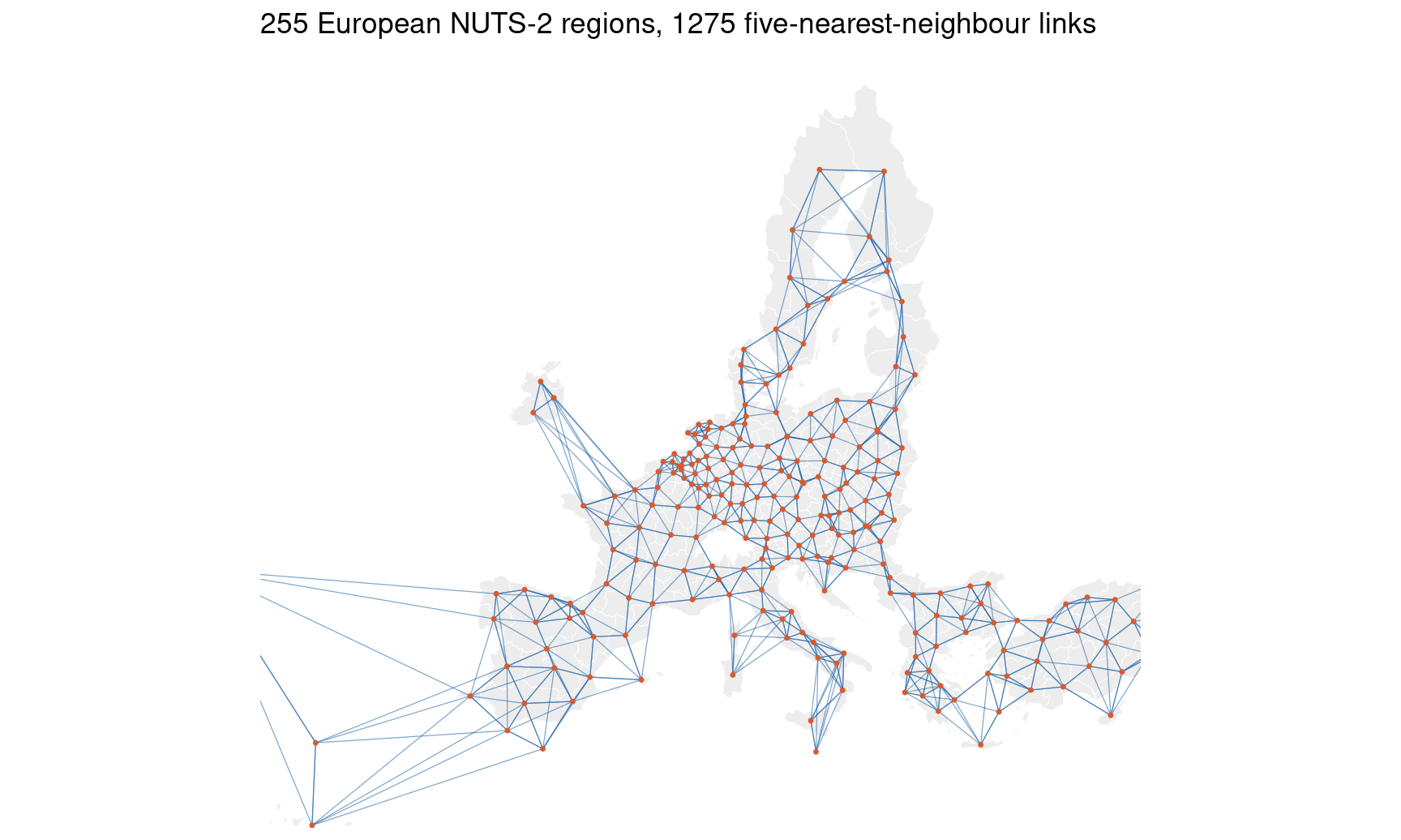
The identical matrix drawn on the map: a line joins \(i\) to \(j\) whenever \(w_{ij} > 0\).
The islands are the giveaway. Malta reaches Sicily; the Canaries reach each other and then across open ocean. Contiguity would have left every one of them with no neighbour at all — Part 2 is about that choice.
Cliff & Ord (1973), Spatial Autocorrelation — the Moran and Geary statistics given their modern sampling theory
Anselin (1988), Spatial Econometrics: Methods and Models — the book that named the field; ML estimation and the LM test family. doi:10.1007/978-94-015-7799-1
Tobler (1970), “A computer movie simulating urban growth in the Detroit region”, Economic Geography 46, 234–240 — doi:10.2307/143141
Ord (1975), “Estimation methods for models of spatial interaction”, JASA 70, 120–126 — the eigenvalue trick that made ML feasible. doi:10.1080/01621459.1975.10480272
Kelejian & Prucha (1998), “A generalized spatial two-stage least squares procedure”, J. Real Estate Finance & Economics 17, 99–121 — GS2SLS without normality. doi:10.1023/A:1007707430416
Kelejian & Prucha (2010), “Specification and estimation of spatial autoregressive models with autoregressive and heteroskedastic disturbances”, J. Econometrics 157, 53–67 — doi:10.1016/j.jeconom.2009.10.025
Lee (2004), “Asymptotic distributions of QML estimators for spatial autoregressive models”, Econometrica 72, 1899–1925 — doi:10.1111/j.1468-0262.2004.00558.x
LeSage & Pace (2009), Introduction to Spatial Econometrics — the impacts argument Part 6 is built on. doi:10.1201/9781420064254
Gibbons & Overman (2012), “Mostly pointless spatial econometrics?”, J. Regional Science 52, 172–191 — the identification critique every user of these models should read. doi:10.1111/j.1467-9787.2012.00760.x
Manski (1993), “Identification of endogenous social effects: the reflection problem”, Review of Economic Studies 60, 531–542 — doi:10.2307/2298123
Halleck Vega & Elhorst (2015), “The SLX model”, J. Regional Science 55, 339–363 — the case for starting simple. doi:10.1111/jors.12188
Conley (1999), “GMM estimation with cross sectional dependence”, J. Econometrics 92, 1–45 — the HAC standard errors of Part 8. doi:10.1016/S0304-4076(98)00084-0
Kolak & Anselin (2020), “A spatial perspective on the econometrics of program evaluation”, International Regional Science Review 43, 128–153 — doi:10.1177/0160017619869781
Part 2 — The Weight Matrix
ἀλλʼ εὐκλεές τοι δύο φίλω κεῖσθαι πέλας.
it is honourable, surely, for two friends to lie near each other
Εὐριπίδης, Φοίνισσαι 1659
What \(\mathbf{W}\) claims
\(\mathbf{W}\) is \(N \times N\). Element \(w_{ij}\) answers one question: how much does region \(j\) count, for region \(i\)?
One number per region, summarising its neighbourhood. Everything else in this deck is a claim about how that number enters the model.
Why the diagonal must be zero
Suppose we allowed \(w_{ii} = c > 0\). The model \(\mathbf{y} = \rho \mathbf{W}\mathbf{y} + \mathbf{X}\beta + \varepsilon\) would contain \(\rho c\, y_i\) on the right-hand side, and we could move it across:
Dividing through by \((1 - \rho c)\) gives a model of exactly the same form with rescaled coefficients. The data cannot distinguish \((\rho, \beta, c)\) from \((\rho', \beta', 0)\) — the parameters are not separately identified.
There is a second, more practical reason. The log-likelihood of Part 5 contains \(\ln|\mathbf{I} - \rho\mathbf{W}|\), and the parameter space for \(\rho\) is set by the eigenvalues of \(\mathbf{W}\). A non-zero diagonal shifts every eigenvalue, so the usual bounds no longer describe where the likelihood is defined.
The same logic explains why spdep, libpysal and Stata’s spmatrix all silently enforce a zero diagonal: it is not a convention, it is a condition for the model to mean anything.
Contiguity: rook or queen
Two regions are neighbours if their boundaries touch. Borrowing from chess:
Rook — they must share a border segment of positive length
Queen — sharing a single point is enough
\[w_{ij} = \begin{cases} 1 & \text{if } i \text{ and } j \text{ share a boundary} \\ 0 & \text{otherwise} \end{cases}\]
On a raster grid this matters enormously: a cell has 4 rook neighbours and 8 queen neighbours, so the choice doubles the neighbourhood. On real administrative regions it barely matters at all, because exact point-contacts are rare. Our 255 European regions:
Four links out of 1088. The textbook distinction is close to irrelevant here, and reporting it as a robustness check is theatre. The choices that do move results are on the next two slides.
Distance-based weights
When contiguity is unavailable or unattractive — point data, islands, regions of wildly different size — build \(\mathbf{W}\) from centroid distances \(d_{ij}\).
Everything is a neighbour, weighted by proximity. \(\alpha = 1\) for gravity-style decay, \(\alpha = 2\) for a physical analogy. Usually combined with a cutoff, or \(\mathbf{W}\) is dense and every eigenvalue computation becomes \(O(N^3)\) with no zeros to exploit.
Simple, and brutally sensitive to \(\bar{d}\). Too small and dense regions cluster while remote ones become islands; too large and the matrix fills in. On our data a 300 km band gives 3888 links, 800 km gives 18906 — nearly five times as many, for a threshold nobody can defend from theory.
\[w_{ij} = \begin{cases} 1 & \text{if } j \text{ is among } i\text{'s } k \text{ closest} \\ 0 & \text{otherwise}\end{cases}\]
Guarantees every region has exactly \(k\) neighbours — no islands, ever. That is why this deck uses it as the primary specification.
The price is that \(\mathbf{W}\) becomes asymmetric: \(j\) can be among \(i\)’s five nearest without \(i\) being among \(j\)’s. On our data 265 of 1275 links are one-way. Dense cities have crowded neighbourhoods; remote regions reach out much further, and are not reached back.
Kernel weights
A smooth compromise between the distance band’s cliff edge and inverse distance’s infinite reach:
\[w_{ij} = K\!\left( \frac{d_{ij}}{h} \right)\]
with bandwidth \(h\) and a kernel \(K\) that decays to zero. The common choices:
The kernel shape matters much less than \(h\), exactly as in every other nonparametric problem in this series. Two ways to set it:
Fixed bandwidth — the same \(h\) everywhere. Honest about geography, but sparse areas end up with few or no neighbours
Adaptive bandwidth — \(h_i\) is the distance to \(i\)’s \(k\)-th nearest neighbour, so every region gets a comparable neighbourhood. This is kNN with smooth edges
Kernels reappear in Part 8: Conley’s HAC standard errors are exactly a kernel weight applied to the moment conditions rather than to the outcome.
Before standardisation, \((\mathbf{W}\mathbf{y})_i\) is a sum over neighbours, so a region with 10 neighbours gets a mechanically larger spatial lag than one with 2. The coefficient \(\rho\) would then be partly measuring degree.
Now \(\rho\) has a clean reading: the fraction of a neighbourhood’s average outcome that transmits to the region itself. It is comparable across regions with different numbers of neighbours, and comparable across studies.
The bounds become tidy too. The largest eigenvalue of a row-standardised \(\mathbf{W}\) is exactly \(1\), so the upper limit of the parameter space is always \(\rho < 1\).
Symmetry is destroyed. Queen contiguity is symmetric — if \(i\) touches \(j\) then \(j\) touches \(i\). Dividing row \(i\) by \(n_i\) and row \(j\) by \(n_j \neq n_i\) breaks that:
The eigenvalues can be complex, so the Jacobian of Part 5 needs care
Influence is no longer reciprocal. A region with 2 neighbours sends 0.5 to each; a region with 10 sends 0.1. Small, remote regions become disproportionately influential transmitters — an artefact of the normalisation, not of economics
The implied “total influence received” is equalised across regions by assumption, which is a strong claim nobody usually defends
Alternatives exist — spectral normalisation (divide by the largest eigenvalue, which preserves symmetry) and doubly-stochastic scaling. Stata’s spmatrix defaults to spectral, R and PySAL to row. Mixing them silently across languages is a real way to get three different answers.
Building \(\mathbf{W}\) from the shared file
Both matrices were computed once from the GISCO geometry and stored as sparse triplets (i, j, w), where i and j index the 255 regions sorted by NUTS code. Each language now turns that same file into its own native object.
import pandas as pd, numpy as npfrom libpysal.weights import Wwk = pd.read_csv("../data/spat-W-knn.csv")N =255# triplets -> dict of neighbours and weights -> libpysal Wnb, wt = {}, {}for i inrange(1, N +1): sub = wk[wk.i == i] nb[i] = sub.j.tolist() wt[i] = sub.w.tolist()Wk = W(nb, wt, silence_warnings=True)rs = np.array([sum(v) for v in Wk.weights.values()])out = (f"libpysal W built: N = {Wk.n}, non-zeros = {Wk.nonzero}\n"f"row sums : min = {rs.min():.6f}, max = {rs.max():.6f}\n"f"mean degree : {np.mean([len(v) for v in Wk.neighbors.values()]):.2f}")import sys; sys.stdout.write(out +"\n"); sys.stdout.flush()
libpysal W built: N = 255, non-zeros = 1275
row sums    : min = 1.000000, max = 1.000000
mean degree : 5.00
108
Code
quietly import delimited "../data/spat-W-knn.csv", clearmata: ii = st_data(., "i"); jj = st_data(., "j"); vv = st_data(., "w")N = 255 Wk = J(N, N, 0)for (k = 1; k <= rows(ii); k++) Wk[ii[k], jj[k]] = vv[k]end* the sp-format geometry is already spset, and its _ID matches our rowindexquietlyuse"../data/spat-nuts-geom.dta", clearmata: idv = st_data(., "_ID")* normalize(none): the triplets are ALREADY row-standardised.* Stata would otherwise apply spectral normalisation and silently disagree* with R and Python.quietly spmatrix spfrommata Wknn = Wk idv, normalize(none) replacemata: printf("spmatrix built: N = %f, non-zeros = %f\n", N, sum(Wk :!= 0)) printf("row sums : min = %9.6f, max = %9.6f\n",min(rowsum(Wk)), max(rowsum(Wk))) printf("mean degree : %4.2f\n", mean(rowsum(Wk :!= 0)))end
------------------------------------------------- mata (type end to exit) ----------------------------------------------
:     ii = st_data(., "i"); jj = st_data(., "j"); vv = st_data(., "w")

:     N  = 255

:     Wk = J(N, N, 0)

:     for (k = 1; k <= rows(ii); k++) Wk[ii[k], jj[k]] = vv[k]

: end
------------------------------------------------------------------------------------------------------------------------


------------------------------------------------- mata (type end to exit) ----------------------------------------------
:     printf("spmatrix built: N = %f, non-zeros = %f\n", N, sum(Wk :!= 0))
spmatrix built: N = 255, non-zeros = 1275

:     printf("row sums    : min = %9.6f, max = %9.6f\n",
>            min(rowsum(Wk)), max(rowsum(Wk)))
row sums    : min =  1.000000, max =  1.000000

:     printf("mean degree : %4.2f\n", mean(rowsum(Wk :!= 0)))
mean degree : 5.00

: end
------------------------------------------------------------------------------------------------------------------------
Three native objects — listw, libpysal.weights.W, spmatrix — none of which can read the others, all built from one file and reporting 1275 non-zeros and row sums of exactly 1. That agreement is what makes the rest of the deck comparable across tabs.
Islands, and the honest choice
Sixteen of our 255 regions have no queen-contiguity neighbour: Cyprus, Malta, the Canaries, the Azores, Madeira, Åland, Corsica, Sicily, Sardinia, the Balearics, Ceuta, Melilla and four Aegean groups.
An island’s row of \(\mathbf{W}\) is entirely zero. Row-standardisation then divides by zero, and software must choose:
spdep — errors unless you pass zero.policy = TRUE, then sets the row to 0
libpysal — warns about disconnected components and carries on
Stata — an all-zero row simply contributes nothing
A zero row means \((\mathbf{W}\mathbf{y})_i = 0\), so the model asserts that this region’s neighbourhood average outcome is zero — not “unknown”, but zero. That is a substantive and false claim, and it enters the likelihood.
Drop them. Changes the sample, and does so non-randomly: islands are poorer and more peripheral than average, so estimates of convergence are affected in a predictable direction. The paper reports \(N\) and nobody notices
Keep them with zero rows. Preserves \(N\), but embeds the false claim above and makes \(\rho\) harder to interpret
Use a \(\mathbf{W}\) with no islands. kNN guarantees \(k\) neighbours for every region by construction
This deck takes the third option, which is why the primary specification is kNN and contiguity is the robustness check — the reverse of the usual textbook order. The reason is the data, not taste: with contiguity, 16 regions would carry a statement about their neighbours that is false by construction.
\(\mathbf{W}\) is an assumption, not data
The literature reports \(\hat\rho\) to three decimals and the choice of \(\mathbf{W}\) in a footnote. Here is the same statistic — Moran’s I on log GDP per head — under nine different specifications of the same 255 regions.
                     W links moranI     z
      queen contiguity  1088 0.5626 12.16
       rook contiguity  1084 0.5619 12.11
               kNN k=3   765 0.5513 11.66
               kNN k=5  1275 0.5187 14.11
              kNN k=10  2550 0.5079 19.78
           band 300 km  3888 0.5350 17.20
           band 500 km  9194 0.4932 23.67
           band 800 km 18906 0.3753 27.21
 inv. distance <800 km 18906 0.4398 25.51
Read it carefully, because the lesson is not the one usually drawn:
The point estimate is robust. Moran’s I stays between roughly 0.38 and 0.56. Every specification agrees: EU regional income is strongly spatially clustered. A referee demanding “robustness to \(\mathbf{W}\)” gets it here
The precision is not. The \(z\)-statistic runs from about 12 to 27, because the number of links runs from 765 to nearly 19000. More links means a tighter null distribution, not more evidence
That is what propagates. The LM tests of Part 3, which choose the model, are built on exactly this variance. A \(\mathbf{W}\) that doubles the link count can flip which test rejects — and therefore which model you fit — while the underlying dependence is unchanged
Report results under at least two genuinely different \(\mathbf{W}\) — one contiguity, one distance-based — and say so in the text, not the appendix. If they disagree, that is a finding about your data, not a nuisance to be tuned away.
Read it as a correlation between a variable and its own spatial lag. The numerator asks whether \(z_i\) and \(z_j\) carry the same sign for pairs that \(\mathbf{W}\) calls neighbours; the denominator scales by total variance.
For a row-standardised \(\mathbf{W}\), \(S_0 = N\) and it simplifies to
\(I > 0\) means neighbours resemble each other — clustering. \(I < 0\) means they differ — a checkerboard. Note it is not bounded by \(\pm 1\).
Under the null of no spatial association,
\[E[I] = \frac{-1}{N-1}\]
which is slightly negative and not zero — an artefact of using \(\bar{y}\), estimated from the same data. With \(N = 255\) that is \(-0.0039\): negligible here, but not in small samples.
The variance under randomisation depends on the shape of \(\mathbf{W}\) through
\(E[C] = 1\); below 1 means clustering, above 1 means dissimilarity — the opposite direction to \(I\).
The two differ in what they emphasise. Moran’s I is a global cross-product, dominated by observations far from the mean; Geary’s C uses pairwise differences, so it responds more to local, small-scale variation. They usually agree in direction, and when they disagree it is a signal that dependence operates at a different scale than \(\mathbf{W}\) assumes.
Moran’s I — on the data
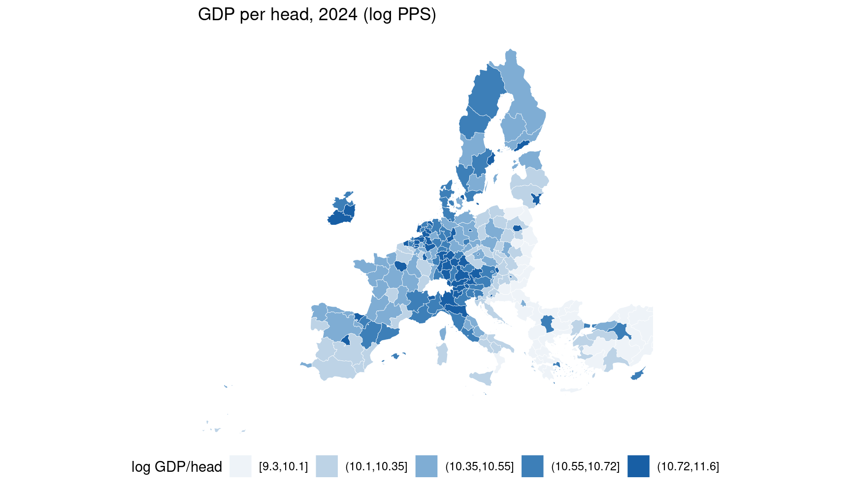
Log GDP per head in 2024, 255 regions, \(k=5\) nearest neighbours.
Moran's I = 0.5187 E[I] = -0.0039 sd = 0.0370 z = 14.11 p = 1.71e-45
Geary's C = 0.4657 E[C] = 1.0000 z = 13.47 p = 1.11e-41
same test on average growth 2000-2024:
Moran's I = 0.7484 z = 20.28 p = 8.86e-92
Code
import numpy as np, pandas as pdfrom libpysal.weights import Wfrom esda import Moran, Gearya = pd.read_csv("../data/spat-nuts.csv")wk = pd.read_csv("../data/spat-W-knn.csv")N =len(a)nb = {i: wk[wk.i == i].j.tolist() for i inrange(1, N +1)}wt = {i: wk[wk.i == i].w.tolist() for i inrange(1, N +1)}Wk = W(nb, wt, silence_warnings=True)y = np.log(a.y1.values)mi = Moran(y, Wk, two_tailed=True)gc = Geary(y, Wk)mg = Moran(a.growth.values, Wk, two_tailed=True)out = (f"Moran's I = {mi.I:8.4f} E[I] = {mi.EI:8.4f} "f"sd = {np.sqrt(mi.VI_norm):.4f} z = {mi.z_norm:6.2f} p = {mi.p_norm:.3g}\n"f"Geary's C = {gc.C:8.4f} E[C] = {gc.EC:8.4f}"f" z = {gc.z_norm:6.2f} p = {gc.p_norm:.3g}\n\n"f"same test on average growth 2000-2024:\n"f"Moran's I = {mg.I:8.4f}"f" z = {mg.z_norm:6.2f} p = {mg.p_norm:.3g}")import sys; sys.stdout.write(out +"\n"); sys.stdout.flush()
Moran's I  =   0.5187   E[I] =  -0.0039   sd = 0.0371   z =  14.10   p = 3.65e-45
Geary's C  =   0.4657   E[C] =   1.0000                z = -13.54   p = 4.4e-42

same test on average growth 2000-2024:
Moran's I  =   0.7484                                z =  20.30   p = 1.24e-91
281
Code
quietly import delimited "../data/spat-W-knn.csv", clearmata: ii = st_data(., "i"); jj = st_data(., "j"); vv = st_data(., "w")N = 255 W = J(N, N, 0)for (k = 1; k <= rows(ii); k++) W[ii[k], jj[k]] = vv[k]endquietly import delimited "../data/spat-nuts.csv", clearmata:// global Moran's I with the randomisation variance.// The return type is mandatory when defining a function inside mata:realrowvector moran(realcolvectory, realmatrix W, realscalarN) { z = y :- mean(y) S0 = sum(W)I = (N/S0) * (z' * W * z) / sum(z:^2) EI = -1/(N-1) S1 = 0.5 * sum((W + W'):^2) S2 = sum((rowsum(W) + colsum(W)'):^2) b2 = (sum(z:^4)/N) / ((sum(z:^2)/N)^2) A = N*((N^2 - 3*N + 3)*S1 - N*S2 + 3*S0^2) B = b2*((N^2 - N)*S1 - 2*N*S2 + 6*S0^2) VI = (A - B) / ((N-1)*(N-2)*(N-3)*S0^2) - EI^2return((I, EI, sqrt(VI), (I - EI)/sqrt(VI))) }y = log(st_data(., "y1"))r = moran(y, W, N) printf("Moran's I = %8.4f E[I] = %8.4f sd = %8.4f z = %6.2f\n",r[1], r[2], r[3], r[4]) z = y :- mean(y) num = 0for (i = 1; i <= N; i++)for (j = 1; j <= N; j++) num = num + W[i,j]*(y[i] - y[j])^2 C = ((N-1)*num) / (2*sum(W)*sum(z:^2)) printf("Geary's C = %8.4f E[C] = %8.4f\n", C, 1) g = moran(st_data(., "growth"), W, N) printf("\nsame test on average growth 2000-2024:\n") printf("Moran's I = %8.4f z = %6.2f\n", g[1], g[4])end
------------------------------------------------- mata (type end to exit) ----------------------------------------------
:     ii = st_data(., "i"); jj = st_data(., "j"); vv = st_data(., "w")

:     N  = 255

:     W  = J(N, N, 0)

:     for (k = 1; k <= rows(ii); k++) W[ii[k], jj[k]] = vv[k]

: end
------------------------------------------------------------------------------------------------------------------------


------------------------------------------------- mata (type end to exit) ----------------------------------------------
:     // global Moran's I with the randomisation variance.
:     // The return type is mandatory when defining a function inside mata:
:     real rowvector moran(real colvector y, real matrix W, real scalar N)
>     {
>         z  = y :- mean(y)
>         S0 = sum(W)
>         I  = (N/S0) * (z' * W * z) / sum(z:^2)
>         EI = -1/(N-1)
>         S1 = 0.5 * sum((W + W'):^2)
>         S2 = sum((rowsum(W) + colsum(W)'):^2)
>         b2 = (sum(z:^4)/N) / ((sum(z:^2)/N)^2)
>         A  = N*((N^2 - 3*N + 3)*S1 - N*S2 + 3*S0^2)
>         B  = b2*((N^2 - N)*S1 - 2*N*S2 + 6*S0^2)
>         VI = (A - B) / ((N-1)*(N-2)*(N-3)*S0^2) - EI^2
>         return((I, EI, sqrt(VI), (I - EI)/sqrt(VI)))
>     }

:
:     y = log(st_data(., "y1"))

:     r = moran(y, W, N)

:     printf("Moran's I  = %8.4f   E[I] = %8.4f   sd = %8.4f   z = %6.2f\n",
>            r[1], r[2], r[3], r[4])
Moran's I  =   0.5187   E[I] =  -0.0039   sd =   0.0370   z =  14.11

:
:     z = y :- mean(y)

:     num = 0

:     for (i = 1; i <= N; i++)
>         for (j = 1; j <= N; j++) num = num + W[i,j]*(y[i] - y[j])^2

:     C = ((N-1)*num) / (2*sum(W)*sum(z:^2))

:     printf("Geary's C  = %8.4f   E[C] = %8.4f\n", C, 1)
Geary's C  =   0.4657   E[C] =   1.0000

:
:     g = moran(st_data(., "growth"), W, N)

:     printf("\nsame test on average growth 2000-2024:\n")

same test on average growth 2000-2024:

:     printf("Moran's I  = %8.4f                                z = %6.2f\n", g[1], g[4])
Moran's I  =   0.7484                                z =  20.28

: end
------------------------------------------------------------------------------------------------------------------------
All three agree: \(I = 0.5187\) on levels with \(z = 14.1\), and Geary’s C of \(0.4657\) points the same way. Growth is even more clustered than levels (\(I = 0.7484\), \(z = 20.3\)) — which is already a substantive result, since convergence theory expects poor regions to grow fastest, not for fast growth to cluster.
Permutation inference
The normal approximation above rests on \(\mathbf{W}\)’s shape, on \(N\) being large, and on a kurtosis correction. None of that is needed.
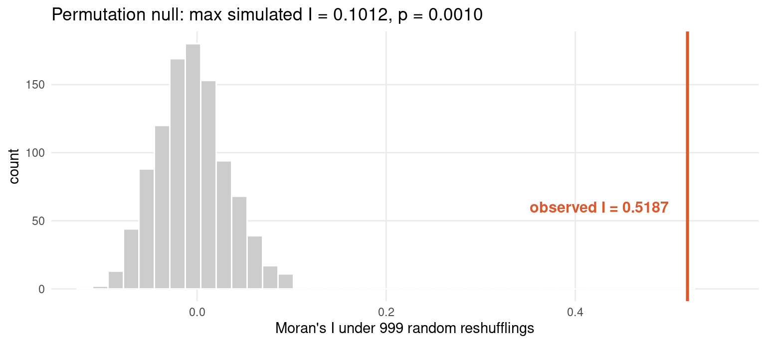
Under the null, spatial arrangement is irrelevant — so shuffle the values across regions and recompute \(I\). Repeat 999 times, and compare the observed \(I\) against that distribution:
The observed \(I\) is not merely in the tail — it is far outside the entire simulated distribution, whose maximum over 999 reshufflings is about \(0.09\). The permutation \(p\) hits its floor of \(1/1000 = 0.001\).
Prefer the permutation test. It makes no distributional assumption, it costs milliseconds, and it degrades gracefully when \(\mathbf{W}\) is irregular or \(y\) is skewed. The normal approximation is a relic of the era when 999 recomputations were expensive. Its one limitation: \(p\) cannot go below \(1/(B+1)\), so report \(p < 0.001\), never \(p = 0\).
LISA — and the multiple-testing problem
A single global \(I\) hides where the clustering is. Local Moran decomposes it region by region (Anselin 1995):
and the global statistic is their average: \(I = \frac{1}{N}\sum_i I_i\).
The sign of \(z_i\) against the sign of its lag \(\sum_j w_{ij} z_j\) classifies each region into one of four quadrants:
High-High — a rich region among rich neighbours (a hot spot)
Low-Low — poor among poor (a cold spot)
High-Low and Low-High — spatial outliers, which are often the interesting cases
You are running 255 hypothesis tests. At \(\alpha = 0.05\) you expect about 13 false positives before looking at the data, and the tests are not independent — neighbouring regions share the observations that go into their statistics. A LISA map at an uncorrected 5% is a map of clusters and of noise, with no way to tell them apart.
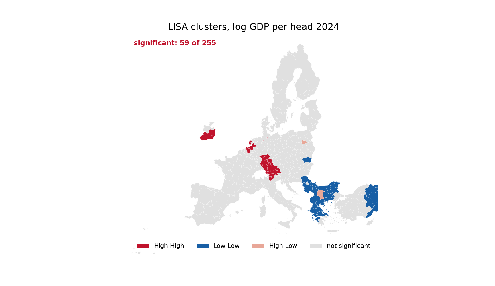
On our data: 59 regions are significant uncorrected, 41 survive a Benjamini–Hochberg FDR correction, and only 22 survive Bonferroni. The map you publish depends on which of those three numbers you use, and most published maps use the first without saying so.
Which correction, and why Bonferroni is usually wrong here
Bonferroni controls the family-wise error rate: the probability of even one false positive. It compares each \(p_i\) against \(\alpha/N\) — here \(0.05/255 = 0.000196\). It is valid under any dependence structure, which is why it survives in a setting where the tests are correlated. It is also brutally conservative: on our data it discards 37 of the 59 flagged regions.
Benjamini–Hochberg controls the false discovery rate: the expected share of false positives among those declared significant. Sort the \(p\)-values ascending and find the largest \(k\) with
\[ p_{(k)} \leq \frac{k}{N}\alpha \]
then reject everything up to \(k\). Here that keeps 41 regions, and the promise is that roughly 5% of those 41 — about two — are spurious.
Which to use. A LISA map is an exploratory device: the goal is to find candidate clusters worth investigating, not to certify each one. Controlling the expected proportion of errors among discoveries is the better match for that goal, so FDR is usually the right choice. Bonferroni is appropriate only when a single false cluster would itself be costly — for example when the map drives a funding allocation.
Two caveats. BH in its original form assumes independence or positive regression dependence; the Benjamini–Yekutieli variant relaxes that at the cost of a \(\ln N\) penalty. And conditional permutation p-values, which resample only the neighbours of each region, are generally better calibrated than the normal approximation used here — at the cost of \(N \times B\) recomputations.
Whatever you choose, state it on the map. “LISA clusters, \(p < 0.05\)” without a correction is not a result; it is 255 tests reported as one.
LISA — the cluster map
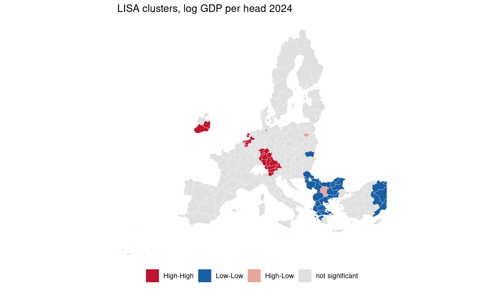
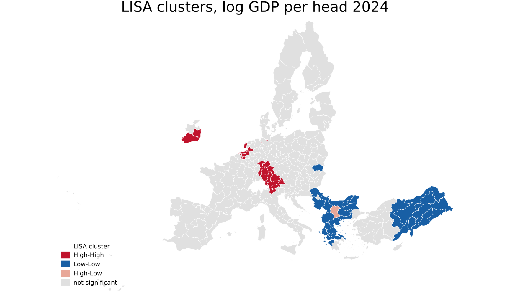
Local Moran on log GDP per head, classified into quadrants, showing only regions significant at an uncorrected 5% so the three maps are comparable. Identical class breaks and identical palette hexes in all three languages.
Code
suppressPackageStartupMessages({library(sf); library(spdep); library(ggplot2)})g <-st_as_sf(read.csv("../data/spat-nuts-wkt.csv"),wkt ="geometry_wkt", crs =3035)# conditional = FALSE gives the classic Anselin (1995) randomisation variance,# which is what the Python and Stata tabs reproduceli <-localmoran(y, lw, conditional =FALSE)lagz <-lag.listw(lw, y -mean(y))g <-transform(g,cluster =ifelse(li[, 5] >=0.05, "not significant",ifelse(y >mean(y) & lagz >0, "High-High",ifelse(y <mean(y) & lagz <0, "Low-Low",ifelse(y >mean(y) & lagz <0, "High-Low", "Low-High")))))pal <-c("High-High"="#C0132C", "Low-Low"="#185FA5","High-Low"="#E8A798", "Low-High"="#9DBBD8","not significant"="grey88")# fix the legend order; a bare character column would sort alphabeticallyg <-transform(g, cluster =factor(cluster, levels =names(pal)))ggplot(g) +aes(fill = cluster) +geom_sf(colour ="white", linewidth =0.12) +scale_fill_manual(values = pal, name =NULL) +coord_sf(xlim =c(1.5e6, 6.6e6), ylim =c(1.0e6, 5.5e6), expand =FALSE) +labs(x =NULL, y =NULL, title ="LISA clusters, log GDP per head 2024") +theme_minimal(base_size =11) +theme(panel.grid =element_blank(), axis.text =element_blank(),legend.position ="bottom")
Code
import numpy as np, pandas as pd, geopandas as gpdimport matplotlib.pyplot as pltfrom matplotlib.patches import Patchfrom shapely import wkt as shwktfrom scipy.stats import normgdf = pd.read_csv("../data/spat-nuts-wkt.csv")gdf = gpd.GeoDataFrame(gdf, geometry=gdf.geometry_wkt.apply(shwkt.loads), crs="EPSG:3035")Wd = np.zeros((N, N))Wd[wk.i -1, wk.j -1] = wk.wz = y - y.mean()m2 = (z **2).sum() / Nlagz = Wd @ zIi = (z / m2) * lagz# the Anselin (1995) randomisation variance, term by termEI =-Wd.sum(axis=1) / (N -1)b2 = ((z **4).sum() / N) / m2 **2wi2 = (Wd **2).sum(axis=1)wikh = Wd.sum(axis=1) **2- wi2VI = (wi2 * (N - b2) / (N -1)+ wikh * (2* b2 - N) / ((N -1) * (N -2)) - EI **2)pval =2* norm.cdf(-np.abs((Ii - EI) / np.sqrt(VI)))cluster = np.where(pval >=0.05, "not significant", np.where((z >0) & (lagz >0), "High-High", np.where((z <0) & (lagz <0), "Low-Low", np.where((z >0) & (lagz <0), "High-Low", "Low-High"))))# "grey" in matplotlib is #808080; R's grey88 and Stata's 224 224 224# are both #E0E0E0, so name the hex explicitly or the three maps divergepal = {"High-High": "#C0132C", "Low-Low": "#185FA5","High-Low": "#E8A798", "Low-High": "#9DBBD8","not significant": "#E0E0E0"}fig, ax = plt.subplots(figsize=(9, 5.2))present = []for lab, col in pal.items(): sub = gdf[cluster == lab]iflen(sub): sub.plot(ax=ax, color=col, edgecolor="white", linewidth=0.12) present.append(Patch(facecolor=col, label=lab))ax.legend(handles=present, loc="lower center", ncol=5, frameon=False, fontsize=8)axopts = ax.set(xlim=(1.5e6, 6.6e6), ylim=(1.0e6, 5.5e6), xticks=[], yticks=[], title="LISA clusters, log GDP per head 2024")ax.text(0.02, 0.95, f"significant: {(pval <0.05).sum()} of {N}", transform=ax.transAxes, fontsize=9, color="#C0132C", weight="bold")ax.set_axis_off()plt.show()
Code
* 1. the shared weightmatrixquietly import delimited "../data/spat-W-knn.csv", clearmata: ii = st_data(., "i"); jj = st_data(., "j"); vv = st_data(., "w")N = 255 W = J(N, N, 0)for (k = 1; k <= rows(ii); k++) W[ii[k], jj[k]] = vv[k]end* 2. the outcome, in the canonical id orderquietly import delimited "../data/spat-nuts.csv", clearmata: y = log(st_data(., "y1"))* 3. local Moran and the Anselin (1995) randomisation variancemata: z = y :- mean(y) m2 = sum(z:^2)/N lagz = W * z Ii = (z :/ m2) :* lagz EI = -rowsum(W) :/ (N-1) b2 = (sum(z:^4)/N) / (m2^2) wi2 = rowsum(W:^2) wikh = rowsum(W):^2 - wi2 VI = wi2 :* (N :- b2) :/ (N-1) :+ /// wikh :* (2*b2 :- N) :/ ((N-1)*(N-2)) :- EI:^2p = 2 :* normal(-abs((Ii - EI) :/ sqrt(VI)))// 1 HH, 2 LL, 3 HL, 4 LH, 5 not significant cl = J(N, 1, 5)for (i = 1; i <= N; i++) {if (p[i] < 0.05) {if (z[i] > 0 & lagz[i] > 0) cl[i] = 1elseif (z[i] < 0 & lagz[i] < 0) cl[i] = 2elseif (z[i] > 0 & lagz[i] < 0) cl[i] = 3else cl[i] = 4 } }end* 4. attach to the sp-format geometry, whose _ID is our id order.* grmap looks for the companion _shp.dta relative to the CURRENT directory,* so move there first; "../plots" then still resolves correctly.quietly cd "../data"quietlyuse"spat-nuts-geom.dta", clearquietlygeneratebyte lisa = .mata: st_store(., st_varindex("lisa"), cl)labeldefine lisalab 1 "High-High" 2 "Low-Low" 3 "High-Low"/// 4 "Low-High" 5 "not significant"labelvalues lisa lisalab* clmethod(unique) assigns colours to the categories that actually OCCUR, in* ascendingorder. No region here is Low-High, so exactly four colours are* supplied - red, blue, pink, grey. Passing five would paint "not significant"* in the Low-High blue.grmap lisa, clmethod(unique) /// fcolor("192 19 44""24 95 165""232 167 152""224 224 224") /// ocolor(white ...) osize(0.02 ...) /// legtitle("LISA cluster") ///title("LISA clusters, log GDP per head 2024")graphexport"../plots/spat-lisa-stata.png", replacewidth(1800)
The picture is the European core–periphery pattern, and it is not subtle: a High-High block running from Ireland through the Low Countries, southern Germany and Austria into northern Italy, and a Low-Low block covering Bulgaria, Romania, eastern Poland, and — most strongly of all — eastern Turkey. Of the 59 significant regions, 25 are High-High, 31 Low-Low, 3 High-Low and none are Low-High.
The LM tests — theory
Moran’s I on residuals tells you dependence is present. It does not tell you whether to fit a lag model or an error model. The Lagrange multiplier tests (Burridge 1980; Anselin 1988) are built for exactly that.
Both start from the OLS residuals only — no spatial model need be estimated, which is what makes them cheap enough to run first.
where \(D = (\mathbf{W}\mathbf{X}\hat{\boldsymbol\beta})'\mathbf{M}(\mathbf{W}\mathbf{X}\hat{\boldsymbol\beta})/s^2 + T\) and \(\mathbf{M}\) is the OLS residual maker.
The two differ only in what the residuals are correlated with: \(\mathbf{W}\mathbf{e}\) for the error test, \(\mathbf{W}\mathbf{y}\) for the lag test.
Each basic test assumes the other form of dependence is absent. If the truth is a lag model, \(LM_{\text{err}}\) still rejects — and vice versa. In practice both reject, and the tests as stated cannot discriminate at all.
The robust versions (Anselin, Bera, Florax & Yoon 1996) correct each test for the possible presence of the other:
\[RLM_{\text{err}} = \frac{\bigl( \mathbf{e}'\mathbf{W}\mathbf{e}/s^2 - T D^{-1}\,\mathbf{e}'\mathbf{W}\mathbf{y}/s^2 \bigr)^2}{T\,(1 - T D^{-1})}\]
Each subtracts off the part of its own statistic that the other form of dependence would have produced. Only the robust pair can discriminate, and reporting the basic pair alone is not enough to choose a model.
There is also a joint test, \(SARMA = RLM_{\text{err}} + LM_{\text{lag}}
\overset{a}{\sim} \chi^2_2\), against “either or both”.
The LM tests — on the data
The convergence regression that Part 7 will estimate properly:
Estimate OLS. Run \(LM_{\text{err}}\) and \(LM_{\text{lag}}\)
Neither rejects → keep OLS, you are done
Exactly one rejects → fit that model
Both reject → go to the robust pair, and fit whichever of \(RLM_{\text{err}}\), \(RLM_{\text{lag}}\) is the more significant
Both robust tests reject → the SAC/SARAR model, or a richer \(\mathbf{W}\)
Our numbers walk straight through it:
Test
Statistic
\(p\)
Verdict
\(LM_{\text{err}}\)
122.25
\(<10^{-27}\)
rejects
\(LM_{\text{lag}}\)
89.67
\(<10^{-20}\)
rejects
\(RLM_{\text{err}}\)
36.39
\(1.6\times10^{-9}\)
rejects decisively
\(RLM_{\text{lag}}\)
3.81
0.051
marginal
Both basic tests reject overwhelmingly and say nothing useful. The robust pair separates cleanly: the error model wins. This is the textbook case, on real data, and it is the exception rather than the rule.
The rule is a decision procedure, not a proof, and it has real limits:
It is a sequence of tests, so it has its own multiple-testing problem. The final model is selected using the same data it is then fitted and tested on, and the reported standard errors ignore that the specification was chosen
A rejection is not identification.\(RLM_{\text{err}}\) rejecting is consistent with a spatially smooth omitted variable, which no spatial error model fixes — it just launders it into \(\lambda\)
Everything is conditional on \(\mathbf{W}\). Part 2 showed the \(z\)-statistic tripling across reasonable choices of \(\mathbf{W}\). The step-4 comparison of \(RLM_{\text{err}}\) against \(RLM_{\text{lag}}\) can flip with it
It never proposes SLX, the simplest spillover model of all, because there is no LM test pointing to it
LeSage and Pace argue the opposite direction entirely — start from the general model and test down. Part 4 puts the two approaches side by side, and Part 7 runs both on this data.
Three places dependence can enter, and each named model switches some of them off:
Model
\(\rho\)
\(\boldsymbol\theta\)
\(\lambda\)
Dependence runs through
OLS
0
0
0
nowhere
SLX
0
free
0
neighbours’ regressors
SAR
free
0
0
neighbours’ outcome
SEM
0
0
free
neighbours’ shocks
SDM
free
free
0
outcome and regressors
SDEM
0
free
free
regressors and shocks
SAC/SARAR
free
0
free
outcome and shocks
Manski
free
free
free
all three — not identified
The rest of this part is about which row you can defend. The short version: the choice is not primarily statistical, and the tests of Part 3 will not settle it on their own.
The outcome in \(i\) depends on the outcomes of \(i\)’s neighbours. This is the model for genuine behavioural interdependence: tax competition, technology diffusion, peer effects.
Solving for \(\mathbf{y}\) shows what has actually been assumed:
Every region’s outcome depends on every region’s regressors, not just its neighbours’, because \((\mathbf{I} - \rho\mathbf{W})^{-1}\) is dense
A shock \(\varepsilon_j\) propagates through the whole system, decaying with network distance
\(\mathbf{W}\mathbf{y}\) is endogenous by construction — it contains \(y_j\), which contains \(\varepsilon_j\), which is correlated with \(\varepsilon_i\) through the same multiplier. OLS is inconsistent, and Part 5 is about the two ways round it.
\(\hat\beta\) in a SAR is not the effect of \(x\) on \(y\). Reporting it as one is the most common error in the applied literature, and Part 6 quantifies it on our own data.
No behavioural spillover at all. Something omitted is spatially smooth — climate, institutions, an unmeasured regional shock — and it shows up in the error:
Why this is the comfortable model, and why that is a warning:
\(\hat{\boldsymbol\beta}\) from OLS remains unbiased and consistent; only efficiency and the standard errors suffer
\(\boldsymbol\beta\) keeps its ordinary reading — the marginal effect of \(x_i\) on \(y_i\), with no impacts machinery needed
Nothing is endogenous, so estimation is a GLS problem
The trap. A SEM does not fix the omitted variable — it absorbs it into \(\lambda\). If that omitted variable is correlated with \(\mathbf{X}\), as spatially smooth things usually are, \(\hat{\boldsymbol\beta}\) is still biased. The SEM buys correct inference about a possibly wrong number.
Neighbours’ characteristics matter; neighbours’ outcomes do not. A region’s growth responds to the human capital next door, not to the growth next door.
Everything about it is easier:
It is OLS. No Jacobian, no likelihood, no endogeneity
\(\boldsymbol\theta\)is the spillover — direct effect \(\beta_k\), indirect effect \(\theta_k\), total \(\beta_k + \theta_k\). No impacts calculation at all
Spillovers are local: the effect stops at the neighbours, so the model does not quietly claim that Portugal affects Estonia
Halleck Vega and Elhorst (2015) argue it should be the default, precisely because the global spillovers of a SAR are an assumption imposed by the functional form rather than something the data asked for.
The cost: if the truth really is an endogenous interaction, SLX is misspecified and \(\boldsymbol\theta\) absorbs a distorted version of it.
The Spatial Durbin Model — SAR plus SLX. It nests SAR (\(\boldsymbol\theta = 0\)), SLX (\(\rho = 0\)) and, under the common factor restriction
\[\boldsymbol{\theta} = -\rho\boldsymbol{\beta}\]
the SEM as well. That last fact is why LeSage and Pace put it at the centre: one model whose restrictions can be tested rather than assumed.
It also has the strongest robustness property. If the true process is a SEM or an SLX, the SDM still yields unbiased estimates of the impacts; the reverse does not hold.
SLX plus a spatial error. Spillovers are local and run through observables; whatever spatial structure remains is nuisance.
Its advantage is interpretive: because \(\rho = 0\), impacts stay trivial — direct \(\beta_k\), indirect \(\theta_k\) — while still allowing spatially correlated unobservables.
Many applied questions are better matched by SDEM than SDM, and it is badly under-used. Choosing between them is choosing between global and local spillovers, which is a question about economics, not about fit.
Endogenous interaction and correlated shocks, with no \(\mathbf{W}\mathbf{X}\) term. Popular because it looks maximally general; it is the model this deck recommends least.
\(\rho\) and \(\lambda\) are weakly identified from one another: both generate spatially smooth \(\mathbf{y}\), and separating them relies entirely on the functional form of the two multipliers. Estimates are often unstable — as the last slide shows on our own data.
The Manski model, and the reflection problem
Turn on all three parameters at once and you have Manski’s (1993) full model, with all three social effects: endogenous (\(\rho\)), contextual (\(\boldsymbol\theta\)) and correlated (\(\lambda\)).
and different \((\rho, \boldsymbol\theta, \lambda)\) triples generate the same reduced form. Manski’s original statement is sharper still: under a linear-in-means structure the endogenous effect cannot be distinguished from the contextual one at all.
The reflection problem, worked through
Manski’s setting: individual \(i\) in group \(g\), with outcome
The group mean outcome is an exact linear function of the group mean characteristic. Substituting it back into the individual equation leaves a regression of \(y_i\) on \(x_i\) and \(\bar{x}_g\) only — two coefficients, from which \(\rho\), \(\theta\) and \(\beta\) cannot all be recovered. The “reflection” is that a person’s behaviour and their group’s average behaviour move together like a mirror image, so neither can be said to cause the other.
What rescues it in the spatial case.\(\mathbf{W}\) is not block-diagonal: neighbourhoods overlap and differ in size. \(i\)’s neighbours and \(j\)’s neighbours are not the same set, so \(\mathbf{W}\mathbf{X}\) and \(\mathbf{W}^2\mathbf{X}\) are not collinear, and identification is restored — from the structure of the network alone.
That is a thin reed. Identification then comes from the exact pattern of who neighbours whom, which is the object Part 2 showed to be an assumption rather than data. Bramoullé, Djebbari and Fortin (2009) give the formal condition: \(\mathbf{I}\), \(\mathbf{W}\) and \(\mathbf{W}^2\) must be linearly independent.
The practical advice follows: do not fit the Manski model. Impose \(\lambda = 0\) (SDM) or \(\rho = 0\) (SDEM), and say which restriction you imposed and why.
Start at OLS. Use the LM tests to decide whether to add anything, and what.
Cheap — everything runs off OLS residuals
Familiar — it is the specification-search logic of most applied work
Risk: each test is computed under a maintained null that is false if the true model is more general, and the sequence has no overall size control
It can never suggest SLX or SDM, because no LM test points at them
Start at the SDM and test the restrictions that would take you somewhere simpler:
\(\boldsymbol\theta = 0\) → SAR
\(\boldsymbol\theta = -\rho\boldsymbol\beta\) → SEM (the common factor restriction)
\(\rho = 0\) → SLX
Robust — if the truth is SEM or SLX, SDM estimates remain consistent, so starting general costs efficiency rather than validity
Coherent — the LR tests are computed under a maintained model that nests every alternative
Cost: you must estimate the general model, which needs the Jacobian of Part 5, and \(\boldsymbol\theta\) is often imprecisely estimated
On our convergence regression the two procedures give different answers:
Procedure
Evidence
Verdict
Test up (Part 3)
\(RLM_{\text{err}} = 36.4\) vs \(RLM_{\text{lag}} = 3.8\)
SEM
Test down
LR vs SAR \(= 32.2\), \(p \approx 10^{-7}\); LR vs SEM \(= 11.3\), \(p = 0.0035\)
SDM
The LM tests say the dependence is a nuisance sitting in the error. The likelihood-ratio tests, run downwards from the SDM, reject both simplifications — including the very SEM the LM tests just recommended.
This is not a contradiction to be settled by picking a favourite test. It is information: the data contain spillovers running through observables (\(\mathbf{W}\mathbf{X}\)) that the LM tests cannot see, because no LM test exists for the SLX component. Part 7 estimates both and reports what changes.
What actually differs
The same convergence regression under six specifications. Watch the coefficient on initial income.
 model  lgdppc0      hcap    rho lambda logLik
   OLS -0.02197 0.0005153     NA     NA  899.1
   SLX -0.01890 0.0006138     NA     NA  911.2
   SAR -0.01219 0.0003598 0.5290     NA  937.6
   SEM -0.01933 0.0006552     NA 0.7016  948.0
   SDM -0.01790 0.0006314 0.6317     NA  953.6
   SAC -0.01880 0.0006328 0.1005 0.6443  948.3
The convergence coefficient runs from \(-0.0220\) under OLS to \(-0.0122\) under SAR — a 44% difference, driven entirely by which model you believe. And the SAR number is not comparable to the others at all, because in a SAR it is not the effect of initial income on growth. That is Part 6.
Note the SAC too: \(\hat\rho = 0.10\) against \(\hat\lambda = 0.64\), with a log-likelihood barely above the SEM’s. The extra parameter buys almost nothing, which is what weak identification looks like in practice.
Part 5 — Estimation: ML and GMM
φάμα Παρνασοῦ τὸν ἄδηλον ἄνδρα πάντʼ ἰχνεύειν.
the voice from Parnassus bids us track the unknown man everywhere
Σοφοκλῆς, Οἰδίπους Τύραννος 474
Why OLS fails for the SAR
Write the SAR as a regression on \(\mathbf{Z} = [\mathbf{W}\mathbf{y}, \mathbf{X}]\). For OLS to be consistent we need \(\mathbf{W}\mathbf{y}\) uncorrelated with \(\boldsymbol{\varepsilon}\). It is not:
The second term contains \(\boldsymbol{\varepsilon}\) directly. Region \(i\)’s neighbours’ outcomes depend on \(i\)’s own shock — through \(i\), back to them — so the regressor and the error move together:
\[\mathrm{plim}\;\frac{1}{N}\,(\mathbf{W}\mathbf{y})'\boldsymbol{\varepsilon}
= \sigma^2\,\mathrm{tr}\!\left[\mathbf{W}(\mathbf{I}-\rho\mathbf{W})^{-1}\right] / N \;\neq\; 0\]
This is simultaneity, exactly as in a system of demand and supply equations, and it does not vanish as \(N\) grows. The bias is upward when \(\rho > 0\) — Part 1 measured it at +42%.
Two routes around it, and this part does both:
Maximum likelihood — write down the density of \(\mathbf{y}\) and maximise it
GMM / instrumental variables — instrument \(\mathbf{W}\mathbf{y}\) with \(\mathbf{W}\mathbf{X}\) and \(\mathbf{W}^2\mathbf{X}\)
Maximum likelihood and the Jacobian
Under normality, \(\boldsymbol{\varepsilon} = (\mathbf{I}-\rho\mathbf{W})\mathbf{y} - \mathbf{X}\boldsymbol{\beta}\). The change of variables from \(\boldsymbol{\varepsilon}\) to \(\mathbf{y}\) carries a Jacobian \(|\mathbf{I} - \rho\mathbf{W}|\), giving
That log-determinant is the whole computational problem. Without it the likelihood would be maximised by driving \(\rho\) towards 1, since shrinking \(\boldsymbol{\varepsilon}\) costs nothing; the Jacobian is what penalises that and makes \(\rho\) identified.
Concentrating out \(\boldsymbol\beta\) and \(\sigma^2\) leaves a one-dimensional problem in \(\rho\):
\[\ln L_c(\rho) = C + \ln\bigl|\mathbf{I} - \rho\mathbf{W}\bigr|
- \frac{N}{2}\ln\bigl[\mathbf{e}(\rho)'\mathbf{e}(\rho)\bigr]\]
where \(\mathbf{e}(\rho) = \mathbf{e}_0 - \rho\,\mathbf{e}_L\) and \(\mathbf{e}_0, \mathbf{e}_L\) are the residuals from regressing \(\mathbf{y}\) and \(\mathbf{W}\mathbf{y}\) on \(\mathbf{X}\). A single scalar optimisation — trivial, provided the determinant is cheap.
Compute the eigenvalues once, at \(O(N^3)\), and every subsequent evaluation over \(\rho\) costs \(O(N)\). This is Ord (1975), and it is why ML became feasible at all.
For our row-standardised kNN matrix, \(\omega_{\max} = 1\) exactly and \(\omega_{\min} = -0.554\), so \(\rho \in (-1.805,\ 1)\).
The limitation is \(N\). At \(N = 255\) the eigen-decomposition is instant; at \(N = 50{,}000\) it is impossible, and the dense matrix will not fit in memory.
For large \(N\), never form eigenvalues. Factor \(\mathbf{I} - \rho\mathbf{W} = \mathbf{L}\mathbf{U}\) with a sparse LU decomposition and read the determinant off the diagonal:
Cost is roughly \(O(N^{1.5})\) for planar graphs, and it exploits the sparsity that contiguity and kNN matrices have in abundance — our kNN matrix is \(1275 / 255^2 = 2\%\) dense. The price is that the factorisation must be redone at every trial \(\rho\).
This is the default in spatialreg for large problems, and the reason method = "eigen" is only the default for small ones.
Both approximate rather than compute.
Chebyshev expands \(\ln|\mathbf{I}-\rho\mathbf{W}|\) in Chebyshev polynomials of \(\mathbf{W}\), needing only matrix–vector products. Monte Carlo (Barry & Pace 1999) uses the trace identity
and estimates each \(\mathrm{tr}(\mathbf{W}^k)\) from random probe vectors.
Both scale to millions of observations. Both introduce approximation error into the likelihood, so the reported standard errors are conditional on the approximation being good — a caveat that is rarely stated.
(The trade-off is the same one the numerical-applications deck makes for linear systems: exact factorisation, sparse factorisation, or iterative approximation, chosen by problem size.)
ML estimation of SAR and SEM
The convergence regression, estimated by maximum likelihood in all three languages from the same weight file.
Code
library(spatialreg)f <- growth ~ lgdppc0 + hcapsar <-lagsarlm(f, data = a, listw = lw) # y = rho W y + X b + esem <-errorsarlm(f, data = a, listw = lw) # u = lambda W u + esummary(sar)summary(sem)
SAR (spatial lag)
rho = 0.52899 (se 0.05442)
lgdppc0 = -0.01219 (se 0.00130)
hcap = 0.00036 (se 0.00005)
logLik = 937.558
SEM (spatial error)
lambda = 0.70163 (se 0.05133)
lgdppc0 = -0.01933 (se 0.00141)
hcap = 0.00066 (se 0.00006)
logLik = 947.989
Code
import numpy as np, pandas as pd, spreg, io, contextlibfrom libpysal.weights import Wa = pd.read_csv("../data/spat-nuts.csv")wk = pd.read_csv("../data/spat-W-knn.csv")N =len(a)nb = {i: wk[wk.i == i].j.tolist() for i inrange(1, N +1)}wt = {i: wk[wk.i == i].w.tolist() for i inrange(1, N +1)}Wk = W(nb, wt, silence_warnings=True)Wk.transform ="r"y = a[["growth"]].valuesX = a[["lgdppc0", "hcap"]].values# spreg echoes the estimator's class name to stdout; keep it off the slidewith contextlib.redirect_stdout(io.StringIO()): sar = spreg.ML_Lag(y, X, w=Wk, name_x=["lgdppc0", "hcap"]) sem = spreg.ML_Error(y, X, w=Wk, name_x=["lgdppc0", "hcap"])# betas is [const, x1, x2, rho] and vm is the matching 4x4, so the spatial# parameter is the LAST entry - vm[-2, -2] would silently give hcap's varianceout = (f"SAR (spatial lag)\n"f" rho = {sar.rho:9.5f} (se {np.sqrt(sar.vm[-1, -1]):.5f})\n"f" lgdppc0 = {sar.betas[1, 0]:9.5f} (se {np.sqrt(sar.vm[1, 1]):.5f})\n"f" hcap = {sar.betas[2, 0]:9.5f} (se {np.sqrt(sar.vm[2, 2]):.5f})\n"f" logLik = {sar.logll:9.3f}\n\n"f"SEM (spatial error)\n"f" lambda = {sem.betas[-1, 0]:9.5f} (se {np.sqrt(sem.vm[-1, -1]):.5f})\n"f" lgdppc0 = {sem.betas[1, 0]:9.5f} (se {np.sqrt(sem.vm[1, 1]):.5f})\n"f" hcap = {sem.betas[2, 0]:9.5f} (se {np.sqrt(sem.vm[2, 2]):.5f})\n"f" logLik = {sem.logll:9.3f}")import sys; sys.stdout.write(out +"\n"); sys.stdout.flush()
The point estimates are identical to five decimals in all three: \(\hat\rho = 0.52899\) with \(\ln L = 937.558\) for the lag model, \(\hat\lambda = 0.70163\) with \(\ln L = 947.989\) for the error model. The error model fits better, as Part 3’s robust LM tests predicted.
The standard errors do not all agree. R and Python report \(\mathrm{se}(\hat\beta_{\ln y_0}) = 0.00130\) and \(z = -9.34\); Stata reports \(0.00123\) and \(z = -9.91\) — about 6% apart, from identical coefficients. The likelihood is the same, so this is a difference in how the asymptotic variance is formed: spatialreg and spreg invert a numerically evaluated information matrix over \((\boldsymbol\beta, \rho, \sigma^2)\), while Stata’s spregress uses its own analytic form. Neither is wrong; they are different finite-sample approximations to the same asymptotic object. Report which software produced an inference, and never mix a coefficient from one with a standard error from another.
GMM and GS2SLS
Maximum likelihood buys efficiency with a normality assumption the data need not honour, and with a determinant that may be unaffordable. Kelejian and Prucha (1998, 1999) give an alternative that needs neither.
They are relevant, because \(\mathbf{W}\mathbf{y}\) is a function of them by construction, and excludable, because \(\mathbf{W}\mathbf{X}\) affects \(y_i\) only through the neighbours’ outcomes — provided the model really is a SAR and not an SDM. If \(\boldsymbol\theta \neq 0\), \(\mathbf{W}\mathbf{X}\) belongs in the equation and is not an instrument at all.
Two-stage least squares on \([\mathbf{W}\mathbf{y}, \mathbf{X}]\) with these instruments is S2SLS. Higher powers add instruments but also weaken them — \(\mathbf{W}^3\mathbf{X}\) is nearly collinear with \(\mathbf{W}^2\mathbf{X}\).
For the SEM, Kelejian and Prucha estimate \(\lambda\) from moment conditions on the residuals rather than a likelihood. With \(\mathbf{u} = \lambda\mathbf{W}\mathbf{u} + \boldsymbol\varepsilon\) and \(\boldsymbol\varepsilon\) i.i.d., three moments identify \(\lambda\) and \(\sigma^2\):
Substituting \(\boldsymbol\varepsilon = \mathbf{u} - \lambda\mathbf{W}\mathbf{u}\) gives three equations that are quadratic in \(\lambda\) — solved by nonlinear least squares, with no distributional assumption anywhere.
Combining the two gives GS2SLS: S2SLS for \(\rho\) and \(\boldsymbol\beta\), the moment estimator for \(\lambda\), then a Cochrane–Orcutt-style transformation and a re-estimation.
ML
GMM / GS2SLS
Normality
assumed
not needed
Heteroskedasticity
breaks it
handled (KP 2010)
Efficiency
efficient if correct
less efficient
Large \(N\)
needs the Jacobian
no determinant at all
Weak instruments
not applicable
a real risk when \(\rho\) is small
The honest summary: ML when \(N\) is moderate and normality is plausible; GMM when it is not, or when \(N\) is large. Report both when they disagree — a large gap is evidence of misspecification, not of a numerical problem.
GS2SLS on the same data
Code
# S2SLS for the lag model: W y instrumented by [X, WX, W^2 X]g_lag <-stsls(f, data = a, listw = lw)# Kelejian-Prucha moment estimator for the error modelg_err <-GMerrorsar(f, data = a, listw = lw)
GS2SLS lag model
rho = 0.30570
lgdppc0 = -0.01632
hcap = 0.00043
GM error model
lambda = 0.41453
lgdppc0 = -0.02111
hcap = 0.00062
for comparison, the ML estimates:
ML lag : rho = 0.52899 lgdppc0 = -0.01219
ML error: lambda = 0.70163 lgdppc0 = -0.01933
Code
with contextlib.redirect_stdout(io.StringIO()): gl = spreg.GM_Lag(y, X, w=Wk, w_lags=2, name_x=["lgdppc0", "hcap"]) ge = spreg.GM_Error(y, X, w=Wk, name_x=["lgdppc0", "hcap"])out = (f"GS2SLS lag model\n"f" rho = {gl.betas[-1, 0]:9.5f}\n"f" lgdppc0 = {gl.betas[1, 0]:9.5f}\n"f" hcap = {gl.betas[2, 0]:9.5f}\n\n"f"GM error model\n"f" lambda = {ge.betas[-1, 0]:9.5f}\n"f" lgdppc0 = {ge.betas[1, 0]:9.5f}\n"f" hcap = {ge.betas[2, 0]:9.5f}\n\n"f"for comparison, the ML estimates:\n"f" ML lag : rho = {sar.rho:9.5f} lgdppc0 = {sar.betas[1, 0]:9.5f}\n"f" ML error: lambda = {sem.betas[-1, 0]:9.5f} lgdppc0 = {sem.betas[1, 0]:9.5f}")import sys; sys.stdout.write(out +"\n"); sys.stdout.flush()
GS2SLS lag model
  rho     =   0.30570
  lgdppc0 =  -0.01632
  hcap    =   0.00043

GM error model
  lambda  =   0.59416
  lgdppc0 =  -0.02015
  hcap    =   0.00065

for comparison, the ML estimates:
  ML lag  : rho    =   0.52899   lgdppc0 =  -0.01219
  ML error: lambda =   0.70163   lgdppc0 =  -0.01933
306
Two things to take from this, and the second is uncomfortable.
The lag model reproduces exactly across all three languages — \(\hat\rho = 0.30570\) and \(\hat\beta_{\ln y_0} = -0.016316\) in R, Python and Stata alike. But it is a long way from the ML estimate of \(\hat\rho = 0.529\). Two consistent estimators of the same parameter should not disagree like this, and the disagreement is informative: it says the SAR is the wrong model, exactly as Part 4 suspected. The instruments \(\mathbf{W}\mathbf{X}\) are invalid when \(\boldsymbol{\theta} \neq 0\), because then they belong in the equation.
The error model does not reproduce across languages. R’s GMerrorsar returns \(\hat\lambda = 0.415\); Python’s spreg.GM_Error returns \(0.594\); and Stata’s gs2sls, errorlag() gives a slope of \(-0.0200\), matching Python’s \(-0.0202\) rather than R’s \(-0.0211\).
This is not a bug in any of them. “The” Kelejian–Prucha estimator is a family: the 1999 original, the 1998 GS2SLS, and the 2010 heteroskedasticity-robust version weight the three moment conditions differently and iterate a different number of times. Each package picked a default and rarely says which. Always name the variant, not just the acronym — and never compare a \(\hat\lambda\) from one package with a \(\hat\lambda\) from another. The ML estimates, by contrast, agree to five decimals everywhere, because there the objective function is unambiguous.
Which estimator recovers \(\rho\)?
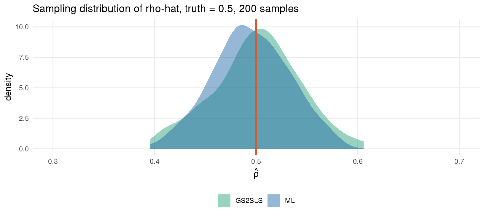
The real data cannot answer this, because nobody knows the truth. The simulated sample can: it was generated as a pure SAR with \(\rho = 0.5\), \(\boldsymbol\beta = (1, -0.8)\) and \(\sigma = 0.5\).
       estimator    rho    b1      b2
           truth 0.5000 1.000 -0.8000
 OLS (ignores W)     NA 1.119 -0.8903
              ML 0.4921 1.035 -0.8231
          GS2SLS 0.5202 1.030 -0.8193
OLS, which does not even have a \(\rho\), mis-estimates both slopes. ML and GS2SLS both land close to the truth. One sample cannot rank them — for that we need the sampling distribution.
 estimator   mean      bias      sd    rmse
        ML 0.4948 -0.005156 0.03718 0.03744
    GS2SLS 0.5006  0.000572 0.04233 0.04223
The textbook trade-off, visible. ML carries a small downward bias (\(\approx -0.005\)) but a tighter distribution; GS2SLS is essentially unbiased and about 14% more variable. Under correct specification and normal errors — exactly the conditions of this simulation — ML wins on RMSE, which is what efficiency means.
Change the conditions and the ranking changes. That is the argument for reporting both.
        model  lgdppc0      hcap    rho lambda logLik
          OLS -0.02197 0.0005153     NA     NA  899.1
     SAR (ML) -0.01219 0.0003598 0.5290     NA  937.6
     SEM (ML) -0.01933 0.0006552     NA 0.7016  948.0
     SDM (ML) -0.01790 0.0006314 0.6317     NA  953.6
 SAR (GS2SLS) -0.01632 0.0004255 0.3057     NA     NA
     SEM (GM) -0.02111 0.0006158     NA 0.4145     NA
Read the lgdppc0 column and remember: for OLS, SEM and SLX it is a marginal effect; for SAR and SDM it is not. Comparing those numbers across rows, as this table invites you to, is the error Part 6 exists to correct.
\begin{table}[htbp]\centering\caption{Convergence regressions, 255 European NUTS-2 regions, $k=5$ nearest neighbours}\begin{tabular}{lccccc}\hlineModel &$\ln y_{2000}$& Human capital &$\rho$&$\lambda$&$\ln L$\\\hlineOLS &$-0.02197$&$0.000515$&&& 899.12 \\SAR (ML) &$-0.01219$&$0.000360$&$0.5290$&& 937.56 \\SEM (ML) &$-0.01933$&$0.000655$&&$0.7016$& 947.99 \\SDM (ML) &$-0.01790$&$0.000631$&$0.6317$&& 953.65 \\SAR (GS2SLS) &$-0.01632$&$0.000425$&$0.3057$&&\\SEM (GM) &$-0.02111$&$0.000616$&&$0.4145$&\\\hline\end{tabular}\begin{tablenotes}\small\item Dependent variable: average annual log growth of GDP per head, 2000--2024.\item For SAR and SDM the reported coefficients are \emph{not} marginal effects; see the impacts table.\end{tablenotes}\end{table}
Part 6 — Impacts
τοιάδʼ ἐρεμνὴ σῖγʼ ἐπέρχεται φάτις.
such a dark report goes about in silence
Σοφοκλῆς, Ἀντιγόνη 700
\(\hat\beta\) is not the effect
In OLS, \(\beta_k = \partial y_i / \partial x_{ik}\). One number, one meaning, and every habit you have about reading a regression table rests on it.
In a SAR that equation is false. Differentiate the reduced form
The \((i,i)\) element is the effect of \(x_{ik}\) on \(y_i\) — not\(\beta_k\)
The \((i,j)\) element is the effect of \(x_{jk}\) on \(y_i\) — not zero
There are \(N^2\) partial derivatives, and \(\beta_k\) is none of them
A SAR or SDM coefficient table is not a table of effects. It is a table of parameters, from which effects must still be computed. Reporting \(\hat\beta_k\) as “the effect of \(x_k\)” is the single most common error in applied spatial econometrics, and the last slide of this part prices it on our own data.
The multiplier, and the feedback loop
Why is \(\partial y_i / \partial x_{ik} \neq \beta_k\)? Expand the inverse as a Neumann series, valid whenever \(|\rho| < 1\) for a row-standardised \(\mathbf{W}\):
\(\mathbf{I}\) — the initial effect on region \(i\) itself, \(\beta_k\)
\(\rho\mathbf{W}\) — \(i\) changes, so \(i\)’s neighbours change
\(\rho^2\mathbf{W}^2\) — the neighbours change, so their neighbours change, and \(\mathbf{W}^2\) has a non-zero diagonal, so some of that comes back to \(i\)
and so on, decaying geometrically in \(\rho\)
That return trip is the feedback loop, and it is why the own-region effect exceeds \(\beta_k\). It is also why the spillover is global: \(\mathbf{W}^m\) eventually connects every pair of regions, so a change anywhere affects everywhere.
How big is the feedback, and how far does it travel?
Take the row-standardised case, where every row of \(\mathbf{W}\) sums to 1. Then every row of \(\mathbf{W}^m\) also sums to 1, and summing the whole series gives the total impact in closed form:
With \(\hat\rho = 0.63\), the multiplier \(1/(1-\rho)\) is about 2.7: the system-wide response to a uniform change in \(x_k\) is nearly three times the coefficient. This is the number people have in mind when they say “the spillovers matter”, and for a pure SAR it is exact.
How much comes back? The own-region effect is \(\frac{1}{N}\mathrm{tr}\!\left[(\mathbf{I}-\rho\mathbf{W})^{-1}\right]\beta_k\). Since \(\mathrm{tr}(\mathbf{W}) = 0\) and \(\mathrm{tr}(\mathbf{W}^2) > 0\), the leading correction is
The \(\rho^2\) term is the shortest possible round trip: out to a neighbour and straight back. For our kNN matrix \(\mathrm{tr}(\mathbf{W}^2)/N = 0.158\) and \(\mathrm{tr}(\mathbf{W}^3)/N = 0.068\), and summing the whole series at \(\hat\rho = 0.632\) gives \(\frac{1}{N}\mathrm{tr}[(\mathbf{I}-\rho\mathbf{W})^{-1}] = 1.107\). So feedback inflates the own-region effect by about 11% — real, and much smaller than the total multiplier of 2.7.
How far? Contributions decay as \(\rho^m\) against a path length \(m\). At \(\rho = 0.63\), five steps carry \(0.63^5 \approx 0.10\) of the initial impulse and ten steps \(0.01\). So “global” is true in principle and modest in practice — which is exactly the point Halleck Vega and Elhorst press when they argue the global structure is an assumption of the SAR functional form rather than a finding.
Direct, indirect, total
\(\mathbf{S}_k(\mathbf{W})\) has \(N^2\) entries. LeSage and Pace summarise it in three scalars.
Direct — the average own-region effect, including feedback that leaves and returns. This is what \(\beta_k\) was supposed to be
Indirect — the average total effect on all other regions. The spillover
Total — what happens if \(x_k\) changes everywhere at once
Each is an average over regions, because in a spatial model the effect genuinely differs by region: a well-connected region has more feedback than a peripheral one. Reporting the average is a summary, not the whole truth.
Computing impacts
The SDM on the convergence regression. All three tabs build \(\mathbf{S}_k(\mathbf{W})\) from the same definition, so the numbers must agree exactly.
Code
sdm <-lagsarlm(growth ~ lgdppc0 + hcap, data = a, listw = lw, type ="mixed")# spatialreg does it for you ...impacts(sdm, listw = lw)# ... and this is what it computesAi <-solve(diag(N) - sdm$rho * W)Sk <- Ai %*% (diag(N) * beta_k + W * theta_k)direct <-sum(diag(Sk)) / Ntotal <-sum(Sk) / N
 variable coefficient     direct   indirect      total
  lgdppc0  -0.0178971 -0.0181303 -0.0035175 -0.0216479
     hcap   0.0006314  0.0006097 -0.0003268  0.0002829
Code
import numpy as np, pandas as pd, spreg, io, contextlibfrom libpysal.weights import W as PWa = pd.read_csv("../data/spat-nuts.csv")wk = pd.read_csv("../data/spat-W-knn.csv")N =len(a)nb = {i: wk[wk.i == i].j.tolist() for i inrange(1, N +1)}wt = {i: wk[wk.i == i].w.tolist() for i inrange(1, N +1)}Wk = PW(nb, wt, silence_warnings=True); Wk.transform ="r"Wd = np.zeros((N, N))Wd[wk.i -1, wk.j -1] = wk.wy = a[["growth"]].valuesX = a[["lgdppc0", "hcap"]].valuesWX = Wd @ Xwith contextlib.redirect_stdout(io.StringIO()): sdm = spreg.ML_Lag(y, np.column_stack([X, WX]), w=Wk)b = sdm.betas.ravel()rho = sdm.rhoAi = np.linalg.inv(np.eye(N) - rho * Wd)lines = ["variable coefficient direct indirect total"]for pos, name inenumerate(["lgdppc0", "hcap"]): bk, tk = b[1+ pos], b[3+ pos] # beta_k and theta_k Sk = Ai @ (np.eye(N) * bk + Wd * tk) dir_ = np.trace(Sk) / N tot = Sk.sum() / N lines.append(f"{name:<9}{bk:11.6f}{dir_:9.6f}{tot - dir_:9.6f}{tot:9.6f}")out ="\n".join(lines)import sys; sys.stdout.write(out +"\n"); sys.stdout.flush()
variable  coefficient    direct  indirect     total
lgdppc0     -0.017897 -0.018130 -0.003518 -0.021648
hcap         0.000631  0.000610 -0.000327  0.000283
156
Code
quietly import delimited "../data/spat-W-knn.csv", clearmata: ii = st_data(., "i"); jj = st_data(., "j"); vv = st_data(., "w")N = 255 Wk = J(N, N, 0)for (k = 1; k <= rows(ii); k++) Wk[ii[k], jj[k]] = vv[k]endquietly cd "../data"quietlyuse"spat-nuts-geom.dta", clearmata: idv = st_data(., "_ID")quietly spmatrix spfrommata Wknn = Wk idv, normalize(none) replace* ivarlag() adds the WX terms, making this an SDM rather than a SARquietly spregress growth lgdppc0 hcap, ml dvarlag(Wknn) ivarlag(Wknn: lgdppc0 hcap)estat impact
------------------------------------------------- mata (type end to exit) ----------------------------------------------
:     ii = st_data(., "i"); jj = st_data(., "j"); vv = st_data(., "w")

:     N  = 255

:     Wk = J(N, N, 0)

:     for (k = 1; k <= rows(ii); k++) Wk[ii[k], jj[k]] = vv[k]

: end
------------------------------------------------------------------------------------------------------------------------


progress   : 50% 100%

Average impacts                                 Number of obs     =        255

------------------------------------------------------------------------------
             |            Delta-Method
             |      dy/dx   std. err.      z    P>|z|     [95% conf. interval]
-------------+----------------------------------------------------------------
direct       |
     lgdppc0 |  -.0181303   .0016223   -11.18   0.000    -.0213099   -.0149507
        hcap |   .0006097   .0000625     9.75   0.000     .0004872    .0007322
-------------+----------------------------------------------------------------
indirect     |
     lgdppc0 |  -.0035175   .0027088    -1.30   0.194    -.0088267    .0017916
        hcap |  -.0003268   .0001632    -2.00   0.045    -.0006466   -6.94e-06
-------------+----------------------------------------------------------------
total        |
     lgdppc0 |  -.0216479   .0021764    -9.95   0.000    -.0259135   -.0173822
        hcap |   .0002829   .0001645     1.72   0.086    -.0000396    .0006054
------------------------------------------------------------------------------
Identical in all three, to every digit shown. The estat impact command also reports standard errors, which is the next slide.
Inference for impacts
The impacts are nonlinear functions of \((\rho, \boldsymbol\beta,
\boldsymbol\theta)\), so their standard errors are not in the coefficient table and cannot be read off it. Two routes:
So draw \(R\) parameter vectors from that distribution, recompute the three impacts for each draw, and use the resulting spread. This is what spatialreg::impacts(..., R = 500) does, and what Stata’s estat impact does analytically by the delta method.
It is cheap because \((\mathbf{I} - \rho\mathbf{W})^{-1}\) is the only expensive object, and the traces of \(\mathbf{W}^m\) can be precomputed once and reused across all draws.
Alternatively, linearise. With \(\mathbf{g}(\cdot)\) the mapping from parameters to impacts,
Faster and deterministic, but it relies on the linearisation being good. Near \(\rho \to 1\) the multiplier explodes and \(\mathbf{g}\) is strongly convex, so the delta method understates uncertainty exactly where uncertainty matters most.
Prefer simulation when \(\hat\rho\) is large or its standard error is appreciable. Our \(\hat\rho = 0.63\) with a small standard error is comfortably in the region where the two agree.
 variable quantity  estimate      z      p
  lgdppc0   direct -0.018130 -11.10 0.0000
     hcap   direct  0.000610   9.68 0.0000
  lgdppc0 indirect -0.003518  -1.29 0.1973
     hcap indirect -0.000327  -1.95 0.0512
  lgdppc0    total -0.021648  -9.91 0.0000
     hcap    total  0.000283   1.67 0.0952
The table that changes the conclusion
Human capital in the convergence regression. Read the row, then read the columns.
Quantity
Estimate
\(z\)
Verdict
SDM coefficient \(\hat\beta\)
\(+0.000631\)
—
not an effect
Direct
\(+0.000610\)
\(9.8\)
strongly positive
Indirect
\(-0.000327\)
\(-2.0\)
significantly negative
Total
\(+0.000283\)
\(1.7\)
not significant\((p = 0.086)\)
A researcher reading the coefficient table concludes that tertiary education raises regional growth, with a \(t\)-statistic near 10. That conclusion is half right and the missing half reverses it:
Educating your own population raises your growth — the direct effect is large and precise
It lowers your neighbours’ growth, significantly. A plausible reading is competition for mobile skilled labour: graduates concentrate in the region that attracts them, at the expense of the region next door
Across Europe as a whole the two nearly cancel, and the total effect is statistically indistinguishable from zero
The policy question — “should the EU fund regional higher education to raise growth?” — is answered by the total impact, not the coefficient. On this data the coefficient says yes with near-certainty and the total impact says we cannot tell. Same model, same estimates, opposite advice.
And the convergence term tells the same story more quietly:
Reading the coefficient rather than the total impact understates the speed of convergence by roughly a quarter, and adds about seven years to the implied half-life of regional income differences.
Never report a bare \(\hat\beta\) from a SAR, SDM or SAC as an effect. Report direct, indirect and total, each with a standard error
Report \(\hat\rho\) as what it is — a parameter of the dependence structure, not a spillover magnitude
Say which \(\mathbf{W}\) produced them, and show at least one alternative
If the indirect effect is your finding, check it survives a different \(\mathbf{W}\). Indirect effects are the least robust quantity in this entire framework
The whole apparatus exists because \((\mathbf{I}-\rho\mathbf{W})^{-1}\) is dense. Set \(\rho = 0\) and it collapses:
The coefficients are the impacts. No inverse, no traces, no simulation — and the standard errors come straight from OLS.
This is the strongest practical argument for SLX and SDEM. If your question is “how large is the spillover”, a model that answers it with a coefficient and a \(t\)-statistic is worth serious consideration before one that requires a simulation to interpret.
The trade-off, again: SLX spillovers are local — they stop at the neighbours. SAR and SDM spillovers are global. Choose on economics, and state the choice.
Part 7 — European Regional Growth
χαῖρʼ· ἄξιος γὰρ καὶ σὺ καὶ πόλις σέθεν.
farewell — worthy are you, and worthy your city
Εὐριπίδης, Ἱκέτιδες 1181
The question
Neoclassical growth theory predicts conditional convergence: poorer regions grow faster, holding constant whatever determines their steady state. The standard test regresses average growth on initial income:
and the half-life of an income gap is \(\ln 2 / s\).
Why space cannot be ignored here. Every quantity in that regression is spatially clustered — Part 3 measured Moran’s I at \(0.52\) on levels and \(0.75\) on growth. Worse, the mechanism is spatial: technology diffuses across borders, workers commute, capital follows agglomeration. A convergence regression that assumes regions are independent is assuming away the transmission channel it is trying to measure.
This part runs the whole apparatus on the real data and asks the only question that matters: does any of it change the answer?
Where the money is
Log GDP per head, 2024, in purchasing power standards. Identical class breaks and identical palette hexes in all three languages — set numerically, never left to auto-ranging.
import numpy as np, pandas as pd, geopandas as gpdimport matplotlib.pyplot as pltfrom matplotlib.colors import BoundaryNorm, ListedColormapfrom matplotlib.patches import Patchfrom shapely import wkt as shwkta = pd.read_csv("../data/spat-nuts.csv")gdf = pd.read_csv("../data/spat-nuts-wkt.csv")gdf = gpd.GeoDataFrame(gdf, geometry=gdf.geometry_wkt.apply(shwkt.loads), crs="EPSG:3035")gdf["ly"] = np.log(a.y1.values)brk = [9.3, 10.1, 10.35, 10.55, 10.72, 11.6]pal = ["#EEF3F8", "#BDD3E6", "#7FADD4", "#3D7FB8", "#185FA5"]cmap = ListedColormap(pal)norm = BoundaryNorm(brk, cmap.N)# discrete swatches, labelled exactly as the R and Stata tabs label themlabs = ["[9.3,10.1]", "(10.1,10.35]", "(10.35,10.55]","(10.55,10.72]", "(10.72,11.6]"]fig, ax = plt.subplots(figsize=(9, 5.2))gdf.plot(column="ly", ax=ax, cmap=cmap, norm=norm, edgecolor="white", linewidth=0.12)ax.legend(handles=[Patch(facecolor=c, label=l) for c, l inzip(pal, labs)], title="log GDP/head", loc="lower center", ncol=5, frameon=False, fontsize=8, title_fontsize=9)axopts = ax.set(xlim=(1.5e6, 6.6e6), ylim=(1.0e6, 5.5e6), xticks=[], yticks=[], title="GDP per head, 2024 (log PPS)")ax.set_axis_off()plt.show()
Code
quietly cd "../data"quietlyuse"spat-nuts-geom.dta", clearquietlygeneratedouble ly = ln(y1)* grmap prints the legendusing the variable's displayformat, and doubles* arrive as %24.15f - without this the breaks read 10.350000000000000format ly %4.2fgrmap ly, clmethod(custom) clbreaks(9.3 10.1 10.35 10.55 10.72 11.6) /// fcolor("238 243 248""189 211 230""127 173 212""61 127 184""24 95 165") /// ocolor(white ...) osize(0.02 ...) /// legtitle("log GDP/head") legorder(lohi) ///title("GDP per head, 2024 (log PPS)")graphexport"../plots/spat-gdp-stata.png", replacewidth(1800)
The core–periphery structure is the whole story: a high-income belt from Ireland through the Low Countries, southern Germany and Austria into northern Italy, with income falling towards every edge. This is not noise around a mean — it is the spatial dependence Part 3 measured, and it is what makes the independence assumption untenable.
Where the growth is
The same regions, now coloured by average annual growth 2000–2024. If convergence held simply, this map would be the inverse of the last one.
It broadly is the inverse — the east grows fastest — which is convergence happening. But growth is itself strongly clustered (\(I = 0.75\), higher than for levels). Fast-growing regions sit next to fast-growing regions, which unconditional convergence does not predict and which no non-spatial regression can represent.
The specification ladder
Every model from Part 4, on this data, with the convergence speed each implies.
 model coefficient total_impact speed_pct half_life
   OLS    -0.02197     -0.02197     3.123     22.20
   SLX    -0.01890     -0.02194     3.116     22.24
   SAR    -0.01219     -0.01219     1.440     48.13
   SEM    -0.01933     -0.01933     2.597     26.69
   SDM    -0.01790     -0.01790     2.337     29.67
Two columns, and the gap between them is the entire lesson of Part 6. For OLS, SLX and SEM they coincide. For SAR and SDM they do not, and only the second is an effect.
The preferred model, in three languages
The SDM is what the likelihood-ratio tests selected in Part 4. Here it is estimated in full — including the \(\mathbf{W}\mathbf{X}\) terms that distinguish it from the SAR — from the same weight file in each language.
Code
# type = "mixed" adds the W X terms, turning a SAR into an SDMsdm <-lagsarlm(growth ~ lgdppc0 + hcap, data = a, listw = lw, type ="mixed")summary(sdm)
quietly import delimited "../data/spat-W-knn.csv", clearmata: ii = st_data(., "i"); jj = st_data(., "j"); vv = st_data(., "w")N = 255 Wk = J(N, N, 0)for (k = 1; k <= rows(ii); k++) Wk[ii[k], jj[k]] = vv[k]endquietly cd "../data"quietlyuse"spat-nuts-geom.dta", clearmata: idv = st_data(., "_ID")quietly spmatrix spfrommata Wknn = Wk idv, normalize(none) replace* dvarlag() is the W y term; ivarlag() adds the W X terms. Both together* are what makes this an SDM rather than a SAR.spregress growth lgdppc0 hcap, ml dvarlag(Wknn) ivarlag(Wknn: lgdppc0 hcap)
\(\hat\rho = 0.6317\), and the Durbin terms are what the LM tests of Part 3 could not see: \(\hat\theta\) on initial income is positive\((+0.0099)\) while its own coefficient is negative — rich neighbours are associated with faster growth even after conditioning on own income. The log-likelihood of \(953.6\) beats both the SAR \((937.6)\) and the SEM \((948.0)\), which is the LR evidence Part 4 reported.
Does \(\mathbf{W}\) change the answer?
The SDM re-estimated under four genuinely different weight matrices.
                W links    rho   direct  indirect    total speed_pct
          kNN k=5  1275 0.6317 -0.01813 -0.003518 -0.02165     3.055
 queen contiguity  1088 0.5554 -0.01096 -0.012521 -0.02348     3.455
         kNN k=10  2550 0.7240 -0.01943 -0.001193 -0.02062     2.843
      band 500 km  9194 0.4938 -0.01432 -0.016130 -0.03045     5.467
This is the most important table in the deck, and it says two opposite things at once:
The total impact is robust. It ranges from \(-0.0206\) to \(-0.0235\) across three of the four matrices — and OLS gave \(-0.0220\). The headline convergence result does not depend on \(\mathbf{W}\)
The decomposition is not. The indirect effect runs from \(-0.0012\) (kNN 10) to \(-0.0161\) (500 km band) — a thirteen-fold difference. \(\hat\rho\) moves between \(0.49\) and \(0.72\)
The quantity people report as their finding — the spillover — is the quantity least identified by the data and most determined by the analyst’s choice of \(\mathbf{W}\). The 500 km band is the outlier throughout, and it is also the matrix with the least defensible justification. That is not a coincidence: the denser the matrix, the more of the total effect it can attribute to neighbours.
Two of the five changed, and they are not the ones usually advertised.
The convergence coefficient is essentially untouched. What the spatial analysis actually bought was (a) valid standard errors, and (b) the discovery that human capital’s apparent growth effect is a redistribution between neighbours rather than a net gain.
It would be easy to present this as a triumph for spatial econometrics. It is more interesting than that.
The point estimate of the thing the literature cares most about — the convergence rate — barely moved. Gibbons and Overman (2012) predict exactly this, and they use it to argue that the spatial machinery often adds complexity without adding identification
The inference genuinely needed fixing. Moran’s I on the OLS residuals was \(0.41\) with \(z = 11.6\); those standard errors were not usable
The new finding — the negative indirect effect of human capital — is real under the primary specification, significant at 5%, and it is also the result most sensitive to \(\mathbf{W}\). It should be reported as suggestive, with the sensitivity table beside it
What this design cannot support
Everything above is a description of a cross-section. Four limits, stated plainly because the machinery makes it easy to forget them:
This is not causal. Nothing here is a natural experiment. \(\hat\beta\) is a conditional correlation, and “conditional convergence” describes a cross-section rather than an estimated treatment effect
\(\mathbf{W}\) is assumed exogenous. For pure geography that is defensible; economic proximity plausibly responds to income, and Part 8 returns to it
A negative indirect effect is not evidence of a mechanism. The skilled-labour-competition story is a reading; the model cannot distinguish it from a spatially correlated omitted variable that happens to load on education
The sample includes candidate countries with very different institutions, and the strongest Low-Low cluster is eastern Turkey. Dropping it would move the numbers, and that itself should be reported
Strip out everything the design cannot bear, and this is what is left standing:
European regional incomes did converge over 2000–2024, at roughly 3% a year, and that rate is robust to the specification and to \(\mathbf{W}\)
The OLS standard errors were not usable — Moran’s I on the residuals was \(0.41\) with \(z = 11.6\) — and the spatial models fix them
Regional human capital’s total growth effect cannot be distinguished from zero once neighbours are accounted for, even though its own-region effect is large and precise
The defensible summary sentence: European regional incomes converged at roughly 3% a year over 2000–2024; accounting for spatial dependence leaves that rate essentially unchanged but corrects badly understated standard errors, and reveals that the growth benefit of regional human capital is substantially offset by losses in neighbouring regions.
Part 8 — Panels, Conley, Exercises
ἔρδοι τις ἣν ἕκαστος εἰδείη τέχνην.
let each man practise the craft he knows
Ἀριστοφάνης, Σφῆκες 1431
Spatial panels
With \(T\) periods the same three dependence channels reappear, now alongside fixed effects:
Three things change, and each is a genuine complication:
The incidental-parameters problem returns. Demeaning to remove \(\mu_i\) correlates the transformed \(\mathbf{W}\mathbf{y}\) with the transformed error. The bias is \(O(1/T)\), so it matters exactly in the short panels regional data gives you
\(\mathbf{W}\) is usually assumed time-invariant, which is convenient and rarely true — road networks and trade links change
Dynamics multiply the problem. A model with both \(y_{i,t-1}\) and \(\mathbf{W}\mathbf{y}_t\) has time dependence, space dependence, and space-time dependence (\(\mathbf{W}\mathbf{y}_{t-1}\)), and identifying all three needs either a long panel or strong restrictions
R
Python
Stata
Spatial panel ML
splm::spml()
spreg.Panel_FE_Lag
spxtregress, fe
Spatial panel GMM
splm::spgm()
spreg.GM_Panel_*
spxtregress, gs2sls
Dynamic
splm (limited)
—
xtdpdml (community)
panel-TWFE and panel-OLS-FE-RE own the non-spatial machinery. What follows is what those decks cannot currently do.
Conley standard errors — theory
Sometimes you do not want a spatial model at all. You believe your regression is correctly specified and you simply want standard errors that survive cross-sectional dependence. That is Conley (1999).
The idea is the spatial analogue of Newey–West. Replace the meat of the sandwich with a distance-weighted sum of cross-products:
No model of the dependence is required — no \(\mathbf{W}\), no \(\rho\), no likelihood
Consistent under general forms of spatial correlation, provided dependence dies out with distance
It fixes only the standard errors. If \(\mathbf{W}\mathbf{y}\) belongs in the model, \(\hat{\boldsymbol\beta}\) is still biased and Conley SEs give you a precise interval around the wrong number
It needs a cutoff, and theory does not supply one
Conley is the right tool when dependence is a nuisance, and the wrong tool when it is the object of interest. It is the spatial counterpart of clustering: honest about uncertainty, silent about mechanism.
Conley in practice
The convergence regression, with the Bartlett kernel at a 500 km cutoff. No package is used in any tab — the estimator is eight lines, and hand-coding it is the only way to prove the three languages agree.
Code
a <-read.csv("../data/spat-nuts.csv"); N <-nrow(a)co <-read.csv("../data/spat-coords.csv")# great-circle distance in km between every pair of centroidsrad <- pi /180lat <- co$lat * radlon <- co$lon * radD <-matrix(0, N, N)for (i in1:N) { cosd <-sin(lat[i]) *sin(lat) +cos(lat[i]) *cos(lat) *cos(lon - lon[i]) cosd[cosd >1] <-1 cosd[cosd <-1] <--1 D[i, ] <-6371*acos(cosd)}X <-cbind(1, a$lgdppc0, a$hcap)y <- a$growthXtXi <-solve(t(X) %*% X)b <- XtXi %*%t(X) %*% ye <-as.numeric(y - X %*% b)conley <-function(cutoff) { K <-matrix(pmax(0, 1- D / cutoff), N, N) # Bartlett kernel M <-matrix(0, 3, 3)for (i in1:N) { wgt <- K[i, ] * e[i] * e M <- M +t(X[i, , drop =FALSE]) %*% (wgt %*% X) }sqrt(diag(XtXi %*% M %*% XtXi))}se_ols <-sqrt(diag(XtXi *sum(e^2) / (N -3)))se_con <-conley(500)cat(sprintf(" lgdppc0 hcap\n"))
lgdppc0 hcap
Code
cat(sprintf("OLS se %.6f %.7f\n", se_ols[2], se_ols[3]))
------------------------------------------------- mata (type end to exit) ----------------------------------------------
:     lat = st_data(., "lat") :* (pi()/180)

:     lon = st_data(., "lon") :* (pi()/180)

:     N   = 255

:     cosd = sin(lat) * sin(lat)' :+ (cos(lat) * cos(lat)') :*
>            cos(J(N,1,1) * lon' :- lon * J(1,N,1))

:     cosd = cosd :* (abs(cosd) :<= 1) :+ sign(cosd) :* (abs(cosd) :> 1)

:     D = 6371 :* acos(cosd)

: end
------------------------------------------------------------------------------------------------------------------------


------------------------------------------------- mata (type end to exit) ----------------------------------------------
:     X = J(N,1,1), st_data(., ("lgdppc0", "hcap"))

:     y = st_data(., "growth")

:     XtXi = invsym(cross(X, X))

:     b = XtXi * cross(X, y)

:     e = y - X*b

:
:     cutoff = 500

:     K = (1 :- D :/ cutoff)                     // Bartlett kernel

:     K = K :* (K :> 0)

:     M = X' * (K :* (e * e')) * X

:     secon = sqrt(diagonal(XtXi * M * XtXi))

:     seols = sqrt(diagonal(XtXi :* ((e' * e)/(N - 3))))

:
:     printf("            lgdppc0      hcap\n")
            lgdppc0      hcap

:     printf("OLS se     %9.6f  %9.7f\n", seols[2], seols[3])
OLS se      0.000905  0.0000567

:     printf("Conley 500 %9.6f  %9.7f\n", secon[2], secon[3])
Conley 500  0.001555  0.0000974

:     printf("ratio      %9.2f  %9.2f\n", secon[2]/seols[2], secon[3]/seols[3])
ratio           1.72       1.72

: end
------------------------------------------------------------------------------------------------------------------------
The convergence coefficient’s standard error is 72% larger once spatial dependence is allowed for. Its \(t\)-statistic falls from about \(-24\) to \(-14\) — still overwhelming here, but on a marginal result this is the difference between publishable and not.
The cutoff is a choice
Conley requires \(\bar d\), and theory says only that it should grow with \(N\). Report the sensitivity, always.
The shape is characteristic and worth recognising:
Below about 200 km the kernel captures almost no pairs and the estimate collapses back towards the OLS number — too small a cutoff hides the problem
Between 300 and 1000 km it rises steadily, roughly doubling
Beyond about 1000 km it flattens and then falls, because the number of effectively independent blocks shrinks and the estimator becomes unstable
Practical advice. Choose a cutoff from the economics — the plausible reach of the mechanism — not from the standard errors it produces. Report at least three, including one deliberately large. If the conclusion depends on the cutoff, that is the finding.
The first says regions influence each other; the second says they all respond to something common — a monetary shock, an oil price, an EU-wide policy.
They demand different remedies. A spatial error model applied to a factor structure will estimate a positive \(\lambda\) and remove nothing. Common correlated effects (Pesaran 2006) or interactive fixed effects (Bai 2009) applied to genuine spatial dependence will absorb the very interaction you wanted to measure.
How to tell them apart: a factor structure produces correlation that does not decay with distance — Portugal and Estonia are as correlated as neighbours. Spatial dependence decays. Plot the residual correlation against distance and look.
(panel-TWFE computes the Pesaran CD statistic that detects the presence of either; this deck supplies the spatial remedy, and that deck the factor one.)
Everything in this deck has assumed \(\mathbf{W}\) is fixed and exogenous. For pure geography — shared borders, physical distance — that is defensible.
It stops being defensible the moment \(\mathbf{W}\) is built from anything economic: trade shares, migration flows, input–output links, “economic distance”. Those respond to the outcome, and then \(\mathbf{W}\mathbf{y}\) is endogenous through a second channel that no instrument in Part 5 addresses.
The literature is thin, and honestly so: Qu and Lee (2015) give a control-function approach for a \(\mathbf{W}\) generated by an observed economic variable, and Kelejian and Piras (2014) give an IV treatment. Both need an exclusion restriction on \(\mathbf{W}\)’s determinants, which is usually as hard as the original identification problem.
The practical position: use geographic \(\mathbf{W}\) for identification, and economic \(\mathbf{W}\) only as a robustness check whose limitations you state.
Where the field is moving — away from modelling dependence and towards designing around it:
Partial interference — assume spillovers occur within known clusters and not between them. Restores identification with a design assumption rather than a \(\mathbf{W}\)
Exposure mappings — replace \(\mathbf{W}\mathbf{y}\) with a low-dimensional function of neighbours’ treatments, e.g. the count of treated neighbours, and estimate a dose–response
Spillover-robust estimators — Aronow & Samii (2017) give design-based estimators of direct and indirect effects under a known exposure mapping
Geographic RDD — a boundary as the discontinuity; see regression-discontinuity-design, which owns this material
The common thread: all of them get identification from a design, and treat interference as a nuisance to be bounded rather than a structure to be estimated. This deck’s models get identification from the functional form of \(\mathbf{W}\), which is why Part 2 insisted so heavily that \(\mathbf{W}\) is an assumption.
Exercises — Estimation
Re-estimate the SDM of Part 7 using the queen contiguity matrix with zero.policy = TRUE. Report \(\hat\rho\) and the three impacts of lgdppc0. The 16 islands now have zero rows — explain what that does to their fitted values, and whether it should worry you.
Fit the SDEM (\(\rho = 0\), \(\lambda\) free, \(\mathbf{W}\mathbf{X}\) included) with errorsarlm(..., etype = "emixed"). Compare its indirect effects with the SDM’s. Which model would you defend for this question, and why?
Estimate the SAR by ML and by GS2SLS on the simulated data, varying the true \(\rho\) over \(\{0.2, 0.5, 0.8\}\) with 200 replications each. At which value does the efficiency advantage of ML disappear, and why should it?
The Part 5 table shows ML and GS2SLS disagreeing sharply on the real data (\(0.529\) vs \(0.306\)). Fit the SDM by GS2SLS instead, instrumenting only \(\mathbf{W}\mathbf{y}\) with \(\mathbf{W}^2\mathbf{X}\) and \(\mathbf{W}^3\mathbf{X}\). Does the disagreement shrink? Explain the result in terms of instrument validity.
Compute the impacts of hcap under the SDM for each region separately (the diagonal and row sums of \(\mathbf{S}_k\), not their averages). Map the region-specific direct effects. Which regions have the largest feedback, and what network property explains it?
Exercises — Testing and Weights
Reproduce the Part 2 sensitivity table using Geary’s C instead of Moran’s I. Does the same “estimate robust, precision fragile” pattern hold?
Implement the conditional permutation version of local Moran: for each region, hold \(z_i\) fixed and resample its five neighbours from the remaining \(N-1\) values, 999 times. Compare the resulting cluster map with the analytical one in Part 3. How many regions change status?
The Anselin decision rule picked the SEM; the LR tests picked the SDM. Compute the common factor test of \(\boldsymbol\theta = -\rho\boldsymbol\beta\) directly, as a Wald test on the SDM. Does it reject? Reconcile the three verdicts.
Build a \(\mathbf{W}\) from economic distance — the absolute difference in 2000 log GDP per head, inverted and row-standardised — and redo the Part 3 tests. The results will look strong. Explain, using Part 8’s endogenous-\(\mathbf{W}\) discussion, why they should not be believed.
Compute Conley standard errors for the SDM rather than OLS, at cutoffs of 300, 500 and 1000 km. Since the SDM already models the dependence, what should the ratio to the model-based standard errors be, and what do you actually find?
LeSage & Pace (2009), Introduction to Spatial Econometrics, CRC Press — the standard reference, and the source of the impacts framework of Part 6. doi:10.1201/9781420064254
Anselin (1988), Spatial Econometrics: Methods and Models, Kluwer — still the clearest derivation of the LM tests. doi:10.1007/978-94-015-7799-1
Elhorst (2014), Spatial Econometrics: From Cross-Sectional Data to Spatial Panels, Springer — the best treatment of Part 8’s panel material. doi:10.1007/978-3-642-40340-8
Arbia (2014), A Primer for Spatial Econometrics, Palgrave — gentler, with worked R examples. doi:10.1057/9781137317940
Read these before believing your own results:
Gibbons & Overman (2012), “Mostly pointless spatial econometrics?”, J. Regional Science 52, 172–191 — the identification critique. Their recommendation is to start from a research design, not from a \(\mathbf{W}\). doi:10.1111/j.1467-9787.2012.00760.x
Halleck Vega & Elhorst (2015), “The SLX model”, J. Regional Science 55, 339–363 — why the simplest spillover model deserves to be the default. doi:10.1111/jors.12188
Corrado & Fingleton (2012), “Where is the economics in spatial econometrics?”, J. Regional Science 52, 210–239 — doi:10.1111/j.1467-9787.2011.00726.x
Kelejian & Piras (2014), “Estimation of spatial models with endogenous weighting matrices”, Regional Science and Urban Economics 46, 140–149 — doi:10.1016/j.regsciurbeco.2014.03.005
R — spdep for weights and tests, spatialreg for models and impacts, splm for panels, sphet for heteroskedasticity-robust GMM
Python — PySAL: libpysal for weights, esda for ESDA and LISA, spreg for models, spglm/spint for GLM and interaction
Stata — the native sp suite (spmatrix, spregress, spivregress, spxtregress, estat impact), plus grmap for choropleths
Conley standard errors — conleyreg (R), acreg and ols_spatial_HAC (Stata). All three implement slightly different defaults; check the kernel before comparing
networks-and-trade-analysis — the same adjacency matrix read as a graph
panel-TWFE, panel-OLS-FE-RE — clustering, Pesaran CD, and the non-spatial panel machinery this part extends
computational-trade-models — gravity, which is spatial economics under another name
regression-discontinuity-design — geographic RDD
numerical-applications-for-economics-and-econometrics — the determinant and sparse-factorisation methods behind Part 5’s Jacobian
Thank You
Athanassios Stavrakoudis Applied Informatics and Computational Economics Lab Department of Economics University of Ioannina, Greece