Code
True demand slope on p : -1.000OLS coefficient on p (biased): -0.2452SLS coefficient on p (struct): -1.034Reduced Forms vs Structure, GMM/SMM/Indirect Inference, Dynamic Discrete Choice, Demand, Production, Games, Auctions, Search & Partial Identification
using , &
8 June 2026
library(tidyverse)   # data wrangling and ggplot2
library(AER)         # ivreg() — 2SLS for simultaneous systems
library(gmm)         # gmm() — generalized method of moments
library(prodest)     # Olley-Pakes / Levinsohn-Petrin / ACF production functions
library(BLPestimatoR)# random-coefficients (BLP) demand estimation
library(numDeriv)    # jacobian() — GMM/SMM standard errors
library(parallel) # mclapply() — parallel Monte Carlo* Built-in: ivregress (2sls/gmm), gmm, kdensity, optimize (Mata).
* ssc install prodest // Olley-Pakes / Levinsohn-Petrin / ACF production
* ssc install blp // Berry-Levinsohn-Pakes random-coefficients demand
* Simulation estimators (SMM, NFXP, CCP, indirect inference) have no native
* Stata command; they are done in Mata or, in practice, R / Python / MATLAB.Data are pre-generated
Every dataset lives in ../data/ and is produced once by structural-data.R (Rscript structural-data.R). The slides only read the CSVs and estimate — no data are simulated inside the deck (except the parallel Monte-Carlo capstone, which resimulates on purpose).
Part I: Reduced Form vs Structure
What “structural” means — and why it can answer questions reduced forms cannot
\[ \underbrace{y = X\beta + u}_{\text{reduced form: a fit}} \qquad\text{vs}\qquad \underbrace{\theta = (\text{utility}, \text{cost}, \text{beliefs}, \text{equilibrium})}_{\text{structure: the primitives}} \]
Reduced-form estimates answer “what happened?”; structural estimates answer “what would happen if…?”
Lucas (1976): reduced-form relationships estimated under one policy regime break down when the policy changes, because agents re-optimise.
\[ \frac{\partial\, \mathbb{E}[y \mid x, \text{policy}]}{\partial\, \text{policy}} \neq 0 \]
The original structural problem (Haavelmo 1943; Cowles Commission): price and quantity are set jointly in equilibrium.
\[ \text{Demand:}\quad q = \alpha - \beta\, p + \gamma\, \text{inc} + u_d \] \[ \text{Supply:}\quad q = \delta + \lambda\, p + \varphi\, \text{cost} + u_s \]
cost shifts supply but is excluded from demand → a valid instrument for \(p\) in the demand equation (and inc does the symmetric job for supply)Solving the two equations for the endogenous \((p,q)\) gives the reduced form:
\[ p = \pi_0 + \pi_1\,\text{inc} + \pi_2\,\text{cost} + v_p, \qquad q = \rho_0 + \rho_1\,\text{inc} + \rho_2\,\text{cost} + v_q \]
For \(i = 1,\dots,n\) with \(n = 4000\), true structural parameters
\[ \alpha=10,\ \beta=1.0,\ \gamma=0.5,\qquad \delta=2,\ \lambda=0.8,\ \varphi=0.6 \]
\[ \text{inc}_i \sim \mathcal N(5,1),\quad \text{cost}_i \sim \mathcal N(3,1),\quad u_{d,i},u_{s,i}\overset{\text{iid}}{\sim}\mathcal N(0,1) \]
Equilibrium price clears the two equations, generating endogeneity in \(p\):
\[ p_i = \frac{(\alpha-\delta) + \gamma\,\text{inc}_i - \varphi\,\text{cost}_i + (u_{d,i}-u_{s,i})}{\beta+\lambda} \]
All datasets in this deck are pre-generated by structural-data.R → ../data/structural-supplydemand.csv; every language reads the same file.
inc: biased upward (toward zero) because \(p\) carries \(u_d\)cost (a supply shifter excluded from demand): recovers \(-\beta\)True demand slope on p : -1.000OLS coefficient on p (biased): -0.2452SLS coefficient on p (struct): -1.034import pandas as pd, numpy as np
from linearmodels.iv import IV2SLS
sd = pd.read_csv("../data/structural-supplydemand.csv")
sd = sd.assign(const=1.0)
ols = IV2SLS(sd["q"], sd[["const", "p", "inc"]], None, None).fit()
tsls = IV2SLS(sd["q"], sd[["const", "inc"]], sd[["p"]], sd[["cost"]]).fit()
print(f"True demand slope on p : {-1.0:+.3f}")True demand slope on p : -1.000OLS coefficient on p (biased): -0.2452SLS coefficient on p (struct): -1.034import delimited "../data/structural-supplydemand.csv", clear
quietly destring _all, replace
quietly regress q p inc
display "OLS coefficient on p (biased): " %6.3f _b[p]
quietly ivregress 2sls q inc (p = cost)
display "2SLS coefficient on p (struct): " %6.3f _b[p]
display "True demand slope on p : " %6.3f -1.0(encoding automatically selected: ISO-8859-1)
(4 vars, 4,000 obs)
OLS coefficient on p (biased): -0.245
2SLS coefficient on p (struct): -1.034
True demand slope on p : -1.000
Part II: Moment-Based Estimation
GMM → Simulated Method of Moments → Indirect Inference → EMM
This deck is the survey: GMM, SMM and indirect inference get roughly six slides here. The companion deck Moments-Based Structural Estimation is the deep dive — the same three estimators across thirty slides, on real data, with weak identification and partial identification treated properly.
The model implies population moment conditions that hold only at the true parameter:
\[ \mathbb{E}\!\left[\, g(w_i,\theta_0) \,\right] = 0, \qquad g:\ \dim(g)=m \ \ge\ \dim(\theta)=k \]
GMM replaces the expectation by a sample average and drives it as close to zero as an \(m\times m\) weight matrix \(W\) allows:
\[ \hat\theta_{\text{GMM}} = \arg\min_{\theta}\ \bar g(\theta)' \, W \, \bar g(\theta), \qquad \bar g(\theta) = \frac{1}{n}\sum_{i=1}^n g(w_i,\theta) \]
The efficient weight matrix is the inverse of the moment covariance, \(W^\ast = S^{-1}\) with \(S = \mathbb{E}[g g']\). Two-step feasible GMM:
\[ \text{step 1: } W = I \ \Rightarrow\ \hat\theta^{(1)} \quad\longrightarrow\quad \hat S = \tfrac1n \sum_i g_i \hat\theta^{(1)} g_i \hat\theta^{(1)\prime} \ \Rightarrow\ \text{step 2: } W = \hat S^{-1} \]
Asymptotics with \(G = \mathbb{E}[\partial g/\partial\theta']\):
\[ \sqrt n(\hat\theta - \theta_0)\ \xrightarrow{d}\ \mathcal N\!\big(0,\ (G'S^{-1}G)^{-1}\big), \qquad J = n\,\bar g(\hat\theta)' \hat S^{-1} \bar g(\hat\theta)\ \xrightarrow{d}\ \chi^2_{m-k} \]
A large \(J\) rejects the over-identifying restrictions — evidence the moments (hence the model) are misspecified. Hansen (1982).
We estimate the demand equation \(q = \alpha - \beta p + \gamma\,\text{inc} + u_d\) by GMM using two instruments for the single endogenous \(p\): cost and cost². With \(m=4\) moments (const, inc, cost, cost²) and \(k=3\) parameters, one over-identifying restriction is left — and the J-test checks it.
sd <- read.csv("../data/structural-supplydemand.csv"); sd$cost2 <- sd$cost^2

# moment conditions  E[ Z (q - a - b p - c inc) ] = 0,  Z = (1, inc, cost, cost^2)
g <- function(theta, x) {
  e <- x[, "q"] - theta[1] - theta[2]*x[, "p"] - theta[3]*x[, "inc"]
  cbind(1, x[, "inc"], x[, "cost"], x[, "cost2"]) * e
}
fit <- gmm(g, x = as.matrix(sd), t0 = c(0, 0, 0), type = "twoStep")  # gmm package
J <- specTest(fit)                                                    # over-identification
cat(sprintf("GMM demand slope on p : %+.3f   (true -1.000)\n", coef(fit)[2]))
GMM demand slope on p : -1.035 (true -1.000)J-stat = 0.615, p = 0.433 (1 over-identifying restriction)import pandas as pd
from linearmodels.iv import IVGMM
sd = pd.read_csv("../data/structural-supplydemand.csv").assign(const=1.0, cost2=lambda d: d.cost**2)
gmm = IVGMM(sd["q"], sd[["const", "inc"]], sd[["p"]], sd[["cost", "cost2"]],
weight_type="robust").fit()
print(f"GMM demand slope on p : {gmm.params['p']:+.3f} (true -1.000)")GMM demand slope on p : -1.035 (true -1.000)J-stat = 0.625 on 1 df, p = 0.429(encoding automatically selected: ISO-8859-1)
(4 vars, 4,000 obs)
GMM demand slope on p : -1.035 (true -1.000)
Test of overidentifying restriction:
Hansen's J chi2(1) = .624895 (p = 0.4292)Many structural models can be simulated from primitives but their moments (or likelihood) have no analytic expression: latent variables, high-dimensional integrals, equilibrium objects.
We use one running example whose likelihood is known (a Tobit) so we can check the answers, but we treat it as a black box that we can only simulate:
\[ y_i^\ast = \theta_0 + \theta_1 x_i + \sigma\,\varepsilon_i,\qquad \varepsilon_i\sim\mathcal N(0,1),\qquad y_i = \max(0,\ y_i^\ast) \]
True values \(\theta_0=0.5,\ \theta_1=1.0,\ \sigma=1.0\), with \(x_i\sim\mathcal N(0,1)\) and \(n=2000\). The censoring at zero makes the observed moments nonlinear in \(\theta\). Data prepared by structural-data.R → ../data/structural-latent.csv.
Pick moments \(g(\theta)=\mathbb E[m(y,x)]-\hat m_{\text{data}}\). Estimate them by simulating \(S\) artificial datasets at \(\theta\) and averaging:
\[ \hat\theta_{\text{SMM}} = \arg\min_\theta\ \Big(\hat m_{\text{data}} - \tfrac1S\!\sum_{s=1}^S m\big(y^s(\theta),x\big)\Big)' W \Big(\cdots\Big) \]
Here \(m = \big(\bar y,\ \overline{y x},\ \overline{y^2},\ \overline{\mathbf 1[y=0]}\big)\) — four moments, three parameters.
lat <- read.csv("../data/structural-latent.csv")
y <- lat$y; x <- lat$x; n <- nrow(lat)

m_data <- c(mean(y), mean(y*x), mean(y^2), mean(y == 0))
W  <- diag(1 / (m_data^2 + 1e-6))          # simple diagonal weight
S  <- 20
set.seed(14159)
eps <- matrix(rnorm(n*S), n, S)            # common random numbers, fixed once

sim_moments <- function(par) {
  th0 <- par[1]; th1 <- par[2]; sg <- exp(par[3])   # sigma > 0 via log
  ys  <- pmax(0, th0 + th1*x + sg*eps)              # n x S simulated outcomes
  c(mean(ys), mean(ys*x), mean(ys^2), mean(ys == 0))
}
obj <- function(par) {
  d <- m_data - sim_moments(par)
  as.numeric(t(d) %*% W %*% d)
}
fit <- optim(c(0, 0, log(1)), obj, method = "Nelder-Mead")
est <- c(fit$par[1:2], exp(fit$par[3]))
cat(sprintf("SMM estimates : theta0=%.3f  theta1=%.3f  sigma=%.3f\n", est[1], est[2], est[3]))
SMM estimates : theta0=0.504 theta1=0.904 sigma=1.042True values : theta0=0.500 theta1=1.000 sigma=1.000import numpy as np, pandas as pd
from scipy import optimize
lat = pd.read_csv("../data/structural-latent.csv")
y, x = lat["y"].to_numpy(), lat["x"].to_numpy()
n = len(y)
m_data = np.array([y.mean(), (y*x).mean(), (y**2).mean(), (y == 0).mean()])
W = np.diag(1/(m_data**2 + 1e-6))
S = 20
rng = np.random.default_rng(14159)
eps = rng.standard_normal((n, S)) # common random numbers
def sim_moments(par):
th0, th1, sg = par[0], par[1], np.exp(par[2])
ys = np.maximum(0, th0 + th1*x[:, None] + sg*eps)
return np.array([ys.mean(), (ys*x[:, None]).mean(), (ys**2).mean(), (ys == 0).mean()])
def obj(par):
d = m_data - sim_moments(par)
return d @ W @ d
fit = optimize.minimize(obj, [0, 0, 0.0], method="Nelder-Mead")
est = [fit.x[0], fit.x[1], np.exp(fit.x[2])]
print(f"SMM estimates : theta0={est[0]:.3f} theta1={est[1]:.3f} sigma={est[2]:.3f}")SMM estimates : theta0=0.392 theta1=0.990 sigma=1.192True values : theta0=0.500 theta1=1.000 sigma=1.000import delimited "../data/structural-latent.csv", clear
quietly destring _all, replace
set seed 14159
* No native command: the SMM criterion is written in Mata and given to optimize()
mata:
void smm_eval(todo, p, y, x, eps, W, mdata, val, grad, hess) {
n = rows(y); Sd = cols(eps)
lin = p[1] :+ p[2]:*x // theta0 + theta1 x
ys = (lin*J(1,Sd,1)) :+ exp(p[3]):*eps // n x Sd, exp() keeps sigma > 0
ys = ys :* (ys :> 0) // censoring: max(0, .)
xm = x*J(1,Sd,1); N = n*Sd
msim = (sum(ys)/N \ sum(ys:*xm)/N \ sum(ys:^2)/N \ sum(ys:==0)/N)
d = mdata - msim
val = (d'*W*d)
}
y = st_data(.,"y"); x = st_data(.,"x"); n = rows(y)
mdata = (mean(y) \ mean(y:*x) \ mean(y:^2) \ mean(y:==0))
W = diag(1:/(mdata:^2 :+ 1e-6))
eps = rnormal(n, 20, 0, 1) // 20 common random draws, fixed
M = optimize_init()
optimize_init_evaluator(M, &smm_eval()); optimize_init_evaluatortype(M, "d0")
optimize_init_which(M, "min"); optimize_init_technique(M, "nm")
optimize_init_nmsimplexdeltas(M, J(1,3,0.1)); optimize_init_params(M, (0,0,0))
optimize_init_argument(M, 1, y); optimize_init_argument(M, 2, x)
optimize_init_argument(M, 3, eps); optimize_init_argument(M, 4, W)
optimize_init_argument(M, 5, mdata)
p = optimize(M)
printf("SMM estimates : theta0=%5.3f theta1=%5.3f sigma=%5.3f\n", p[1], p[2], exp(p[3]))
printf("True values : theta0=%5.3f theta1=%5.3f sigma=%5.3f\n", 0.5, 1.0, 1.0)
end(encoding automatically selected: ISO-8859-1)
(2 vars, 2,000 obs)
------------------------------------------------- mata (type end to exit) ----------------------------------------------
: void smm_eval(todo, p, y, x, eps, W, mdata, val, grad, hess) {
> n = rows(y); Sd = cols(eps)
> lin = p[1] :+ p[2]:*x // theta0 + theta1 x
> ys = (lin*J(1,Sd,1)) :+ exp(p[3]):*eps // n x Sd, exp() keeps sigma > 0
> ys = ys :* (ys :> 0) // censoring: max(0, .)
> xm = x*J(1,Sd,1); N = n*Sd
> msim = (sum(ys)/N \ sum(ys:*xm)/N \ sum(ys:^2)/N \ sum(ys:==0)/N)
> d = mdata - msim
> val = (d'*W*d)
> }
note: argument todo unused.
note: argument grad unused.
note: argument hess unused.
: y = st_data(.,"y"); x = st_data(.,"x"); n = rows(y)
: mdata = (mean(y) \ mean(y:*x) \ mean(y:^2) \ mean(y:==0))
: W = diag(1:/(mdata:^2 :+ 1e-6))
: eps = rnormal(n, 20, 0, 1) // 20 common random draws, fixed
: M = optimize_init()
: optimize_init_evaluator(M, &smm_eval()); optimize_init_evaluatortype(M, "d0")
: optimize_init_which(M, "min"); optimize_init_technique(M, "nm")
: optimize_init_nmsimplexdeltas(M, J(1,3,0.1)); optimize_init_params(M, (0,0,0))
: optimize_init_argument(M, 1, y); optimize_init_argument(M, 2, x)
: optimize_init_argument(M, 3, eps); optimize_init_argument(M, 4, W)
: optimize_init_argument(M, 5, mdata)
: p = optimize(M)
Iteration 0: f(p) = 1.9367799
Iteration 1: f(p) = .48948456
Iteration 2: f(p) = .21399492
Iteration 3: f(p) = .21399492
Iteration 4: f(p) = .21399492
Iteration 5: f(p) = .21399492
Iteration 6: f(p) = .21399492
Iteration 7: f(p) = .21399492
Iteration 8: f(p) = .21399492
Iteration 9: f(p) = .17664306
Iteration 10: f(p) = .17664306
Iteration 11: f(p) = .17664306
Iteration 12: f(p) = .1643534
Iteration 13: f(p) = .13675639
Iteration 14: f(p) = .13675639
Iteration 15: f(p) = .13675639
Iteration 16: f(p) = .13675639
Iteration 17: f(p) = .08320836
Iteration 18: f(p) = .08320836
Iteration 19: f(p) = .06349008
Iteration 20: f(p) = .04440225
Iteration 21: f(p) = .02499267
Iteration 22: f(p) = .0228119
Iteration 23: f(p) = .01991768
Iteration 24: f(p) = .01991768
Iteration 25: f(p) = .01763951
Iteration 26: f(p) = .01730628
Iteration 27: f(p) = .01643262
Iteration 28: f(p) = .01643262
Iteration 29: f(p) = .01603372
Iteration 30: f(p) = .01493307
Iteration 31: f(p) = .01493307
Iteration 32: f(p) = .01369579
Iteration 33: f(p) = .01369579
Iteration 34: f(p) = .01073358
Iteration 35: f(p) = .01073358
Iteration 36: f(p) = .01068423
Iteration 37: f(p) = .00569104
Iteration 38: f(p) = .00569104
Iteration 39: f(p) = .00569104
Iteration 40: f(p) = .00355994
Iteration 41: f(p) = .00340933
Iteration 42: f(p) = .00186576
Iteration 43: f(p) = .00041891
Iteration 44: f(p) = .00041891
Iteration 45: f(p) = .00037879
Iteration 46: f(p) = .00030567
Iteration 47: f(p) = .00030567
Iteration 48: f(p) = .00023437
Iteration 49: f(p) = .00012199
Iteration 50: f(p) = .00012199
Iteration 51: f(p) = .00010365
Iteration 52: f(p) = .00010365
Iteration 53: f(p) = .00010365
Iteration 54: f(p) = .00009884
Iteration 55: f(p) = .00008935
Iteration 56: f(p) = .00008935
Iteration 57: f(p) = .00008935
Iteration 58: f(p) = .00008863
Iteration 59: f(p) = .00008863
Iteration 60: f(p) = .00008826
Iteration 61: f(p) = .00008795
Iteration 62: f(p) = .00008795
Iteration 63: f(p) = .00008795
Iteration 64: f(p) = .00008795
Iteration 65: f(p) = .00008787
Iteration 66: f(p) = .00008787
Iteration 67: f(p) = .00008785
Iteration 68: f(p) = .00008763
Iteration 69: f(p) = .00008763
Iteration 70: f(p) = .00008763
Iteration 71: f(p) = .00008763
: printf("SMM estimates : theta0=%5.3f theta1=%5.3f sigma=%5.3f\n", p[1], p[2], exp(p[3]))
SMM estimates : theta0=0.499 theta1=0.966 sigma=1.032
: printf("True values : theta0=%5.3f theta1=%5.3f sigma=%5.3f\n", 0.5, 1.0, 1.0)
True values : theta0=0.500 theta1=1.000 sigma=1.000
: end
------------------------------------------------------------------------------------------------------------------------Choose an auxiliary model that is easy to estimate (here: OLS of \(y\) on \(x\) plus the residual SD). Fit it once to the real data to get \(\hat\beta\). Then find the structural \(\theta\) whose simulated data reproduce the same auxiliary estimates:
\[ \hat\theta_{\text{II}} = \arg\min_\theta \big(\hat\beta_{\text{data}} - \tilde\beta(\theta)\big)' W \big(\hat\beta_{\text{data}} - \tilde\beta(\theta)\big) \]
lat <- read.csv("../data/structural-latent.csv")
y <- lat$y; x <- lat$x; n <- nrow(lat)

aux <- function(yy, xx) {                 # auxiliary estimator: OLS + resid SD
  m <- lm(yy ~ xx)
  c(coef(m), log(sd(residuals(m))))
}
b_data <- aux(y, x)

S <- 20
set.seed(14159)
x_big   <- rep(x, S)
eps_big <- rnorm(n*S)                     # common random numbers, fixed once
obj <- function(par) {
  th0 <- par[1]; th1 <- par[2]; sg <- exp(par[3])
  ys <- pmax(0, th0 + th1*x_big + sg*eps_big)
  d  <- b_data - aux(ys, x_big)
  sum(d^2)
}
fit <- optim(c(0, 0, 0), obj, method = "Nelder-Mead")
est <- c(fit$par[1:2], exp(fit$par[3]))
cat(sprintf("Indirect inference : theta0=%.3f  theta1=%.3f  sigma=%.3f\n", est[1], est[2], est[3]))
Indirect inference : theta0=0.537 theta1=0.888 sigma=1.010True values : theta0=0.500 theta1=1.000 sigma=1.000import numpy as np, pandas as pd
from scipy import optimize
lat = pd.read_csv("../data/structural-latent.csv")
y, x = lat["y"].to_numpy(), lat["x"].to_numpy()
n = len(y)
def aux(yy, xx): # OLS slope/intercept + log resid SD
Xd = np.column_stack([np.ones_like(xx), xx])
b, *_ = np.linalg.lstsq(Xd, yy, rcond=None)
resid = yy - Xd @ b
return np.array([b[0], b[1], np.log(resid.std(ddof=2))])
b_data = aux(y, x)
S = 20
rng = np.random.default_rng(14159)
x_big = np.tile(x, S)
eps_big = rng.standard_normal(n*S) # common random numbers
def obj(par):
th0, th1, sg = par[0], par[1], np.exp(par[2])
ys = np.maximum(0, th0 + th1*x_big + sg*eps_big)
d = b_data - aux(ys, x_big)
return d @ d
fit = optimize.minimize(obj, [0, 0, 0.0], method="Nelder-Mead")
est = [fit.x[0], fit.x[1], np.exp(fit.x[2])]
print(f"Indirect inference : theta0={est[0]:.3f} theta1={est[1]:.3f} sigma={est[2]:.3f}")Indirect inference : theta0=0.519 theta1=0.947 sigma=1.018True values : theta0=0.500 theta1=1.000 sigma=1.000import delimited "../data/structural-latent.csv", clear
quietly destring _all, replace
set seed 14159
mata:
real colvector aux(yy, xx) { // auxiliary: OLS + log resid SD
n = rows(yy); Xd = (J(n,1,1), xx)
b = invsym(Xd'Xd)*(Xd'yy)
resid = yy - Xd*b
return((b \ ln(sqrt(sum(resid:^2)/(n-2)))))
}
void ii_eval(todo, p, xbig, epsbig, bdata, val, grad, hess) {
ys = p[1] :+ p[2]:*xbig :+ exp(p[3]):*epsbig
ys = ys :* (ys :> 0)
d = bdata - aux(ys, xbig) // match auxiliary estimates
val = sum(d:^2)
}
y = st_data(.,"y"); x = st_data(.,"x"); n = rows(y)
bdata = aux(y, x)
xbig = J(20,1,1) # x // 20 common random datasets
epsbig = rnormal(n*20, 1, 0, 1)
M = optimize_init()
optimize_init_evaluator(M, &ii_eval()); optimize_init_evaluatortype(M, "d0")
optimize_init_which(M, "min"); optimize_init_technique(M, "nm")
optimize_init_nmsimplexdeltas(M, J(1,3,0.1)); optimize_init_params(M, (0,0,0))
optimize_init_argument(M, 1, xbig); optimize_init_argument(M, 2, epsbig)
optimize_init_argument(M, 3, bdata)
p = optimize(M)
printf("Indirect inference : theta0=%5.3f theta1=%5.3f sigma=%5.3f\n", p[1], p[2], exp(p[3]))
printf("True values : theta0=%5.3f theta1=%5.3f sigma=%5.3f\n", 0.5, 1.0, 1.0)
end(encoding automatically selected: ISO-8859-1)
(2 vars, 2,000 obs)
------------------------------------------------- mata (type end to exit) ----------------------------------------------
: real colvector aux(yy, xx) { // auxiliary: OLS + log resid SD
> n = rows(yy); Xd = (J(n,1,1), xx)
> b = invsym(Xd'Xd)*(Xd'yy)
> resid = yy - Xd*b
> return((b \ ln(sqrt(sum(resid:^2)/(n-2)))))
> }
: void ii_eval(todo, p, xbig, epsbig, bdata, val, grad, hess) {
> ys = p[1] :+ p[2]:*xbig :+ exp(p[3]):*epsbig
> ys = ys :* (ys :> 0)
> d = bdata - aux(ys, xbig) // match auxiliary estimates
> val = sum(d:^2)
> }
note: argument todo unused.
note: argument grad unused.
note: argument hess unused.
: y = st_data(.,"y"); x = st_data(.,"x"); n = rows(y)
: bdata = aux(y, x)
: xbig = J(20,1,1) # x // 20 common random datasets
: epsbig = rnormal(n*20, 1, 0, 1)
: M = optimize_init()
: optimize_init_evaluator(M, &ii_eval()); optimize_init_evaluatortype(M, "d0")
: optimize_init_which(M, "min"); optimize_init_technique(M, "nm")
: optimize_init_nmsimplexdeltas(M, J(1,3,0.1)); optimize_init_params(M, (0,0,0))
: optimize_init_argument(M, 1, xbig); optimize_init_argument(M, 2, epsbig)
: optimize_init_argument(M, 3, bdata)
: p = optimize(M)
Iteration 0: f(p) = .64139675
Iteration 1: f(p) = .26802773
Iteration 2: f(p) = .26802773
Iteration 3: f(p) = .26802773
Iteration 4: f(p) = .26802773
Iteration 5: f(p) = .25729132
Iteration 6: f(p) = .23963635
Iteration 7: f(p) = .18583457
Iteration 8: f(p) = .18583457
Iteration 9: f(p) = .18583457
Iteration 10: f(p) = .18583457
Iteration 11: f(p) = .16830071
Iteration 12: f(p) = .16830071
Iteration 13: f(p) = .16830071
Iteration 14: f(p) = .14975784
Iteration 15: f(p) = .12948534
Iteration 16: f(p) = .12948534
Iteration 17: f(p) = .08033286
Iteration 18: f(p) = .08033286
Iteration 19: f(p) = .04415181
Iteration 20: f(p) = .01726118
Iteration 21: f(p) = .01726118
Iteration 22: f(p) = .00627006
Iteration 23: f(p) = .00627006
Iteration 24: f(p) = .00513719
Iteration 25: f(p) = .00488921
Iteration 26: f(p) = .00479167
Iteration 27: f(p) = .00472116
Iteration 28: f(p) = .00472084
Iteration 29: f(p) = .00472084
Iteration 30: f(p) = .00464625
Iteration 31: f(p) = .00464625
Iteration 32: f(p) = .00461231
Iteration 33: f(p) = .00447224
Iteration 34: f(p) = .00447224
Iteration 35: f(p) = .00426598
Iteration 36: f(p) = .00405912
Iteration 37: f(p) = .00387257
Iteration 38: f(p) = .00313163
Iteration 39: f(p) = .00313163
Iteration 40: f(p) = .0025666
Iteration 41: f(p) = .0014231
Iteration 42: f(p) = .00087409
Iteration 43: f(p) = .00087409
Iteration 44: f(p) = .00020921
Iteration 45: f(p) = .00020921
Iteration 46: f(p) = .00020921
Iteration 47: f(p) = .00020921
Iteration 48: f(p) = .00012976
Iteration 49: f(p) = .0000552
Iteration 50: f(p) = .00002737
Iteration 51: f(p) = 5.443e-06
Iteration 52: f(p) = 3.838e-06
Iteration 53: f(p) = 6.361e-07
Iteration 54: f(p) = 6.361e-07
Iteration 55: f(p) = 3.297e-07
Iteration 56: f(p) = 3.297e-07
Iteration 57: f(p) = 1.412e-08
Iteration 58: f(p) = 1.412e-08
Iteration 59: f(p) = 1.412e-08
: printf("Indirect inference : theta0=%5.3f theta1=%5.3f sigma=%5.3f\n", p[1], p[2], exp(p[3]))
Indirect inference : theta0=0.529 theta1=0.941 sigma=1.004
: printf("True values : theta0=%5.3f theta1=%5.3f sigma=%5.3f\n", 0.5, 1.0, 1.0)
True values : theta0=0.500 theta1=1.000 sigma=1.000
: end
------------------------------------------------------------------------------------------------------------------------EMM is indirect inference whose moments are the score of the auxiliary model, evaluated at the auxiliary MLE \(\hat\beta\) but averaged over simulated data:
\[ m(\theta) = \frac1S\sum_{s} \frac{\partial \log f_{\text{aux}}}{\partial\beta}\Big(y^s(\theta),x;\ \hat\beta\Big),\qquad \hat\theta_{\text{EMM}} = \arg\min_\theta\ m(\theta)'\, \hat I^{-1}\, m(\theta) \]
lat <- read.csv("../data/structural-latent.csv")
y <- lat$y; x <- lat$x; n <- nrow(lat)

# Auxiliary: Gaussian linear model y ~ N(b0 + b1 x, s^2). MLE = OLS.
m0 <- lm(y ~ x); bhat <- coef(m0); s2 <- mean(residuals(m0)^2)

score <- function(yy, xx) {                # per-obs auxiliary scores at bhat, s2
  r  <- yy - (bhat[1] + bhat[2]*xx)
  cbind(r/s2, (r*xx)/s2, -1/(2*s2) + r^2/(2*s2^2))
}
Ihat <- crossprod(score(y, x)) / n         # information = score covariance
Winv <- solve(Ihat)

S <- 20
set.seed(14159)
x_big <- rep(x, S); eps_big <- rnorm(n*S)
obj <- function(par) {
  th0 <- par[1]; th1 <- par[2]; sg <- exp(par[3])
  ys <- pmax(0, th0 + th1*x_big + sg*eps_big)
  m  <- colMeans(score(ys, x_big))         # simulated average score
  as.numeric(t(m) %*% Winv %*% m)
}
fit <- optim(c(0, 0, 0), obj, method = "Nelder-Mead")
est <- c(fit$par[1:2], exp(fit$par[3]))
cat(sprintf("EMM estimates : theta0=%.3f  theta1=%.3f  sigma=%.3f\n", est[1], est[2], est[3]))
EMM estimates : theta0=0.538 theta1=0.887 sigma=1.010True values : theta0=0.500 theta1=1.000 sigma=1.000import numpy as np, pandas as pd
from scipy import optimize
lat = pd.read_csv("../data/structural-latent.csv")
y, x = lat["y"].to_numpy(), lat["x"].to_numpy()
n = len(y)
Xd = np.column_stack([np.ones_like(x), x])
bhat, *_ = np.linalg.lstsq(Xd, y, rcond=None)
s2 = ((y - Xd @ bhat)**2).mean()
def score(yy, xx):
r = yy - (bhat[0] + bhat[1]*xx)
return np.column_stack([r/s2, r*xx/s2, -1/(2*s2) + r**2/(2*s2**2)])
Winv = np.linalg.inv(score(y, x).T @ score(y, x) / n)
S = 20
rng = np.random.default_rng(14159)
x_big = np.tile(x, S); eps_big = rng.standard_normal(n*S)
def obj(par):
th0, th1, sg = par[0], par[1], np.exp(par[2])
ys = np.maximum(0, th0 + th1*x_big + sg*eps_big)
m = score(ys, x_big).mean(axis=0)
return m @ Winv @ m
fit = optimize.minimize(obj, [0, 0, 0.0], method="Nelder-Mead")
est = [fit.x[0], fit.x[1], np.exp(fit.x[2])]
print(f"EMM estimates : theta0={est[0]:.3f} theta1={est[1]:.3f} sigma={est[2]:.3f}")EMM estimates : theta0=0.520 theta1=0.946 sigma=1.018True values : theta0=0.500 theta1=1.000 sigma=1.000import delimited "../data/structural-latent.csv", clear
quietly destring _all, replace
set seed 14159
mata:
real matrix score(yy, xx, b0, b1, s2) { // auxiliary Gaussian scores
r = yy :- (b0 :+ b1:*xx)
return((r:/s2, (r:*xx):/s2, (-1/(2*s2)) :+ (r:^2):/(2*s2^2)))
}
void emm_eval(todo, p, xbig, epsbig, b0, b1, s2, Winv, val, grad, hess) {
ys = p[1] :+ p[2]:*xbig :+ exp(p[3]):*epsbig
ys = ys :* (ys :> 0)
m = (mean(score(ys, xbig, b0, b1, s2)))' // simulated average score
val = (m'*Winv*m)
}
y = st_data(.,"y"); x = st_data(.,"x"); n = rows(y)
Xd = (J(n,1,1), x); bh = invsym(Xd'Xd)*(Xd'y); s2 = mean((y - Xd*bh):^2)
Sc0 = score(y, x, bh[1], bh[2], s2)
Winv = luinv((Sc0'Sc0)/n) // efficient weight = info matrix
xbig = J(20,1,1) # x; epsbig = rnormal(n*20, 1, 0, 1)
M = optimize_init()
optimize_init_evaluator(M, &emm_eval()); optimize_init_evaluatortype(M, "d0")
optimize_init_which(M, "min"); optimize_init_technique(M, "nm")
optimize_init_nmsimplexdeltas(M, J(1,3,0.1)); optimize_init_params(M, (0,0,0))
optimize_init_argument(M, 1, xbig); optimize_init_argument(M, 2, epsbig)
optimize_init_argument(M, 3, bh[1]); optimize_init_argument(M, 4, bh[2])
optimize_init_argument(M, 5, s2); optimize_init_argument(M, 6, Winv)
p = optimize(M)
printf("EMM estimates : theta0=%5.3f theta1=%5.3f sigma=%5.3f\n", p[1], p[2], exp(p[3]))
printf("True values : theta0=%5.3f theta1=%5.3f sigma=%5.3f\n", 0.5, 1.0, 1.0)
end(encoding automatically selected: ISO-8859-1)
(2 vars, 2,000 obs)
------------------------------------------------- mata (type end to exit) ----------------------------------------------
: real matrix score(yy, xx, b0, b1, s2) { // auxiliary Gaussian scores
> r = yy :- (b0 :+ b1:*xx)
> return((r:/s2, (r:*xx):/s2, (-1/(2*s2)) :+ (r:^2):/(2*s2^2)))
> }
: void emm_eval(todo, p, xbig, epsbig, b0, b1, s2, Winv, val, grad, hess) {
> ys = p[1] :+ p[2]:*xbig :+ exp(p[3]):*epsbig
> ys = ys :* (ys :> 0)
> m = (mean(score(ys, xbig, b0, b1, s2)))' // simulated average score
> val = (m'*Winv*m)
> }
note: argument todo unused.
note: argument grad unused.
note: argument hess unused.
: y = st_data(.,"y"); x = st_data(.,"x"); n = rows(y)
: Xd = (J(n,1,1), x); bh = invsym(Xd'Xd)*(Xd'y); s2 = mean((y - Xd*bh):^2)
: Sc0 = score(y, x, bh[1], bh[2], s2)
: Winv = luinv((Sc0'Sc0)/n) // efficient weight = info matrix
: xbig = J(20,1,1) # x; epsbig = rnormal(n*20, 1, 0, 1)
: M = optimize_init()
: optimize_init_evaluator(M, &emm_eval()); optimize_init_evaluatortype(M, "d0")
: optimize_init_which(M, "min"); optimize_init_technique(M, "nm")
: optimize_init_nmsimplexdeltas(M, J(1,3,0.1)); optimize_init_params(M, (0,0,0))
: optimize_init_argument(M, 1, xbig); optimize_init_argument(M, 2, epsbig)
: optimize_init_argument(M, 3, bh[1]); optimize_init_argument(M, 4, bh[2])
: optimize_init_argument(M, 5, s2); optimize_init_argument(M, 6, Winv)
: p = optimize(M)
Iteration 0: f(p) = 1.1143965
Iteration 1: f(p) = .66965599
Iteration 2: f(p) = .1290163
Iteration 3: f(p) = .1290163
Iteration 4: f(p) = .1290163
Iteration 5: f(p) = .11013129
Iteration 6: f(p) = .08805638
Iteration 7: f(p) = .0855137
Iteration 8: f(p) = .08249236
Iteration 9: f(p) = .05154504
Iteration 10: f(p) = .05154504
Iteration 11: f(p) = .05154504
Iteration 12: f(p) = .03746967
Iteration 13: f(p) = .03746967
Iteration 14: f(p) = .033879
Iteration 15: f(p) = .02279568
Iteration 16: f(p) = .02279568
Iteration 17: f(p) = .01966759
Iteration 18: f(p) = .01814237
Iteration 19: f(p) = .01810327
Iteration 20: f(p) = .01791896
Iteration 21: f(p) = .01773267
Iteration 22: f(p) = .01736959
Iteration 23: f(p) = .01645616
Iteration 24: f(p) = .01568258
Iteration 25: f(p) = .01568258
Iteration 26: f(p) = .01280597
Iteration 27: f(p) = .01280597
Iteration 28: f(p) = .01280597
Iteration 29: f(p) = .0081743
Iteration 30: f(p) = .0081743
Iteration 31: f(p) = .00634267
Iteration 32: f(p) = .00147245
Iteration 33: f(p) = .00147245
Iteration 34: f(p) = .00147245
Iteration 35: f(p) = .00147245
Iteration 36: f(p) = .00126735
Iteration 37: f(p) = .00005898
Iteration 38: f(p) = .00005898
Iteration 39: f(p) = .00002657
Iteration 40: f(p) = 5.760e-06
Iteration 41: f(p) = 5.760e-06
Iteration 42: f(p) = 3.296e-06
Iteration 43: f(p) = 1.655e-06
Iteration 44: f(p) = 3.654e-07
Iteration 45: f(p) = 3.654e-07
Iteration 46: f(p) = 3.066e-08
Iteration 47: f(p) = 3.066e-08
Iteration 48: f(p) = 1.639e-08
Iteration 49: f(p) = 2.751e-09
: printf("EMM estimates : theta0=%5.3f theta1=%5.3f sigma=%5.3f\n", p[1], p[2], exp(p[3]))
EMM estimates : theta0=0.529 theta1=0.941 sigma=1.003
: printf("True values : theta0=%5.3f theta1=%5.3f sigma=%5.3f\n", 0.5, 1.0, 1.0)
True values : theta0=0.500 theta1=1.000 sigma=1.000
: end
------------------------------------------------------------------------------------------------------------------------
Part III: Dynamic Discrete Choice
Rust’s nested fixed point — and the Hotz–Miller CCP shortcut
An agent observes state \(x_t\) and choice-specific shocks \(\varepsilon_t\), picks \(a_t\in\{0,1\}\) to maximise expected discounted utility:
\[ \max_{\{a_t\}}\ \mathbb E\sum_{t=0}^{\infty}\beta^t\big[u(x_t,a_t) + \varepsilon_t(a_t)\big] \]
The choice-specific value function (integrating out future \(\varepsilon\)) satisfies Bellman’s equation:
\[ v(x,a) = u(x,a) + \beta\,\mathbb E\big[\, \bar V(x') \mid x,a \,\big],\qquad \bar V(x) = \mathbb E_\varepsilon \max_a\{v(x,a)+\varepsilon(a)\} \]
With \(\varepsilon(a)\) iid Type-I Extreme Value, the \(\max\) integrates in closed form (log-sum) and choice probabilities are multinomial logit:
\[ \bar V(x) = \log\sum_{a}\exp v(x,a) + \text{const}, \qquad P(a\mid x) = \frac{\exp v(x,a)}{\sum_{a'}\exp v(x,a')} \]
Harold Zurcher decides each month whether to replace a bus engine (\(a=1\)) or keep it (\(a=0\)), given mileage \(x\):
\[ u(x,0) = -\theta_1 x \quad(\text{rising maintenance cost}), \qquad u(x,1) = -RC \quad(\text{fixed replacement}) \]
\(K=20\) mileage bins, mileage increments \(j\in\{0,1,2\}\) with probabilities \((0.35,0.45,0.20)\), discount \(\beta=0.9\). True parameters \(\theta_1=0.05\), \(RC=4\). structural-data.R solves the value-function fixed point, then simulates \(N=100\) buses for \(T=100\) months → ../data/structural-rust.csv (columns bus, t, x, replace).
\[ v_0(x) = -\theta_1 x + \beta\,\mathbb E[\bar V(x')\mid x,\text{keep}], \quad v_1(x) = -RC + \beta\,\mathbb E[\bar V(x')\mid 0,\text{keep}] \]
solve_ev) — these are structure, not dataRust’s NFXP nests two loops:
\[ \hat\theta_{\text{NFXP}} = \arg\max_\theta \sum_{i}\log P(a_i\mid x_i;\theta), \qquad P(1\mid x;\theta) = \frac{\exp v_1(x)}{\exp v_0(x)+\exp v_1(x)} \]
# Model primitives (structure, shared with the CCP slide via the R session)
K <- 20; beta <- 0.9; p_incr <- c(0.35, 0.45, 0.20)
states <- 0:K; S <- length(states)
F <- matrix(0, S, S)                             # transition under KEEP
for (i in 1:S) for (j in 0:2) { dest <- min(i + j, S); F[i, dest] <- F[i, dest] + p_incr[j + 1] }
solve_ev <- function(theta1, RC) {               # inner fixed point (contraction)
  EV <- numeric(S)
  repeat {
    v0 <- -theta1*states + beta*(F %*% EV)
    v1 <- -RC + beta*sum(F[1, ]*EV)              # replace: continue from state 0
    EVn <- log(exp(v0) + exp(v1))
    if (max(abs(EVn - EV)) < 1e-12) break
    EV <- EVn
  }
  list(pr_replace = as.numeric(plogis(v1 - v0)))
}

rust <- read.csv("../data/structural-rust.csv")
xi <- rust$x + 1L; di <- rust$replace

negll <- function(par) {
  theta1 <- par[1]; RC <- par[2]
  if (theta1 <= 0 || RC <= 0) return(1e10)
  pr   <- solve_ev(theta1, RC)$pr_replace
  prob <- pmin(pmax(pr[xi], 1e-12), 1 - 1e-12)
  -sum(di*log(prob) + (1 - di)*log(1 - prob))
}
fit <- optim(c(0.10, 3.0), negll, method = "L-BFGS-B",
             lower = c(1e-3, 1e-3), upper = c(1, 20))
cat(sprintf("NFXP estimates : theta1=%.4f   RC=%.3f\n", fit$par[1], fit$par[2]))
NFXP estimates : theta1=0.0494 RC=3.930True values : theta1=0.0500 RC=4.000import numpy as np, pandas as pd
from scipy import optimize
K, beta = 20, 0.9
p_incr = np.array([0.35, 0.45, 0.20])
states = np.arange(K + 1); S = K + 1
F = np.zeros((S, S))
for i in range(S):
for j in range(3):
F[i, min(i + j, S - 1)] += p_incr[j]
def solve_ev(theta1, RC):
EV = np.zeros(S)
while True:
v0 = -theta1*states + beta*(F @ EV)
v1 = -RC + beta*(F[0] @ EV)
EVn = np.log(np.exp(v0) + np.exp(v1))
if np.max(np.abs(EVn - EV)) < 1e-12:
break
EV = EVn
return 1/(1 + np.exp(v0 - v1)) # P(replace | x)
rust = pd.read_csv("../data/structural-rust.csv")
xi = rust["x"].to_numpy(); di = rust["replace"].to_numpy()
def negll(par):
theta1, RC = par
if theta1 <= 0 or RC <= 0:
return 1e10
pr = np.clip(solve_ev(theta1, RC)[xi], 1e-12, 1 - 1e-12)
return -np.sum(di*np.log(pr) + (1 - di)*np.log(1 - pr))
fit = optimize.minimize(negll, [0.10, 3.0], method="Nelder-Mead")
print(f"NFXP estimates : theta1={fit.x[0]:.4f} RC={fit.x[1]:.3f}")NFXP estimates : theta1=0.0494 RC=3.929True values : theta1=0.0500 RC=4.000import delimited "../data/structural-rust.csv", clear
quietly destring _all, replace
* Rust has no native Stata command: the contraction + ML are written in Mata.
mata:
real colvector solve_ev(real scalar t1, real scalar RC, real matrix F,
real colvector states, real scalar beta) {
S = rows(F); EV = J(S,1,0); diff = 1
while (diff > 1e-12) { // inner fixed point (contraction)
v0 = -t1:*states :+ beta:*(F*EV)
v1 = -RC :+ beta:*(F[1,]*EV); v1s = v1[1,1]
EVn = ln(exp(v0) :+ exp(v1s))
diff = max(abs(EVn - EV)); EV = EVn
}
return(1:/(1:+exp(v0:-v1s))) // P(replace | x)
}
void nfxp_eval(todo, p, F, states, beta, xi, di, val, grad, hess) {
pr = solve_ev(exp(p[1]), exp(p[2]), F, states, beta) // exp() keeps params > 0
prob = pr[xi]
prob = rowmin((rowmax((prob, J(rows(prob),1,1e-12))), J(rows(prob),1,1-1e-12)))
val = sum(di:*ln(prob) :+ (1:-di):*ln(1:-prob)) // outer log-likelihood
}
xi = st_data(., "x") :+ 1; di = st_data(., "replace")
K = 20; beta = 0.9; states = (0::K); S = K+1; p_incr = (0.35, 0.45, 0.20)
F = J(S,S,0)
for (i=1; i<=S; i++) {
for (j=0; j<=2; j++) { dest = min((i+j, S)); F[i,dest] = F[i,dest] + p_incr[j+1] }
}
M = optimize_init()
optimize_init_evaluator(M, &nfxp_eval()); optimize_init_evaluatortype(M, "d0")
optimize_init_which(M, "max"); optimize_init_params(M, (ln(0.1), ln(3)))
optimize_init_argument(M, 1, F); optimize_init_argument(M, 2, states)
optimize_init_argument(M, 3, beta); optimize_init_argument(M, 4, xi)
optimize_init_argument(M, 5, di)
p = optimize(M)
printf("NFXP (Mata) : theta1=%6.4f RC=%6.3f\n", exp(p[1]), exp(p[2]))
printf("True values : theta1=%6.4f RC=%6.3f\n", 0.05, 4.0)
end(encoding automatically selected: ISO-8859-1)
(4 vars, 10,000 obs)
------------------------------------------------- mata (type end to exit) ----------------------------------------------
: real colvector solve_ev(real scalar t1, real scalar RC, real matrix F,
> real colvector states, real scalar beta) {
> S = rows(F); EV = J(S,1,0); diff = 1
> while (diff > 1e-12) { // inner fixed point (contraction)
> v0 = -t1:*states :+ beta:*(F*EV)
> v1 = -RC :+ beta:*(F[1,]*EV); v1s = v1[1,1]
> EVn = ln(exp(v0) :+ exp(v1s))
> diff = max(abs(EVn - EV)); EV = EVn
> }
> return(1:/(1:+exp(v0:-v1s))) // P(replace | x)
> }
: void nfxp_eval(todo, p, F, states, beta, xi, di, val, grad, hess) {
> pr = solve_ev(exp(p[1]), exp(p[2]), F, states, beta) // exp() keeps params > 0
> prob = pr[xi]
> prob = rowmin((rowmax((prob, J(rows(prob),1,1e-12))), J(rows(prob),1,1-1e-12)))
> val = sum(di:*ln(prob) :+ (1:-di):*ln(1:-prob)) // outer log-likelihood
> }
note: argument todo unused.
note: argument grad unused.
note: argument hess unused.
: xi = st_data(., "x") :+ 1; di = st_data(., "replace")
: K = 20; beta = 0.9; states = (0::K); S = K+1; p_incr = (0.35, 0.45, 0.20)
: F = J(S,S,0)
: for (i=1; i<=S; i++) {
> for (j=0; j<=2; j++) { dest = min((i+j, S)); F[i,dest] = F[i,dest] + p_incr[j+1] }
invalid expression
(10 lines skipped)
------------------------------------------------------------------------------------------------------------------------
r(3000);
r(3000);Hotz & Miller (1993): the mapping from choice-specific value differences to conditional choice probabilities (CCPs) is invertible. For binary logit it is startlingly simple:
\[ v_1(x) - v_0(x) = \log P(1\mid x) - \log P(0\mid x) \]
Given data CCPs \(\hat P\), the value function under that policy solves a single linear system (no iteration to a fixed point):
\[ \bar V = \big(I - \beta F_{\hat P}\big)^{-1} \sum_a \hat P_a \odot\big(u_a(\theta) + \gamma - \log \hat P_a\big) \]
where \(F_{\hat P}=\sum_a \operatorname{diag}(\hat P_a)F_a\) is the policy-weighted transition and \(\gamma\) is Euler’s constant. Because \(u_a(\theta)\) is linear in \(\theta=(\theta_1,RC)\), so is \(v_1-v_0\), and the CCP step reduces to a logistic regression — one Newton step, no nested solve. This is the Aguirregabiria–Mira (2002) pseudo-likelihood view of Hotz–Miller.
rust <- read.csv("../data/structural-rust.csv")
# Step 1: empirical CCPs P(replace | x), smoothed for empty cells
tab <- tapply(rust$replace, rust$x, mean)
Phat <- rep(NA, S); Phat[as.integer(names(tab)) + 1] <- tab
Phat[is.na(Phat)] <- mean(rust$replace)
Phat <- pmin(pmax(Phat, 1e-3), 1 - 1e-3)
euler <- 0.5772156649

# policy-weighted transition: keep -> F, replace -> renew from state 0
F0 <- F; F1 <- matrix(rep(F[1, ], each = S), S, S)   # every row = row of state 0
Fp <- (1 - Phat)*F0 + Phat*F1
Minv <- solve(diag(S) - beta*Fp)

# V and v1 - v0 are LINEAR in theta = (theta1, RC): build coefficients by columns.
# flow utilities: u0 = -theta1*x ; u1 = -RC  ->  du/dtheta known, intercept 0.
ent <- euler - ((1 - Phat)*log(1 - Phat) + Phat*log(Phat))   # entropy term
build_vdiff <- function(theta1, RC) {
  u0 <- -theta1*states; u1 <- rep(-RC, S)
  rhs <- (1 - Phat)*(u0 + ent) + Phat*(u1 + ent)
  V   <- Minv %*% rhs
  v0  <- u0 + beta*(F0 %*% V)
  v1  <- u1 + beta*(F1 %*% V)
  as.numeric(v1 - v0)
}
# Because v1 - v0 is linear in (theta1, RC), fit by ML with a 2-column design.
base <- build_vdiff(0, 0)
c_t1 <- build_vdiff(1, 0) - base      # slope wrt theta1
c_rc <- build_vdiff(0, 1) - base      # slope wrt RC
xi <- rust$x + 1L; di <- rust$replace
Xdes <- cbind(c_t1[xi], c_rc[xi]); off <- base[xi]
ccp_fit <- glm(di ~ Xdes - 1 + offset(off), family = binomial())
cat(sprintf("CCP estimates : theta1=%.4f   RC=%.3f\n", coef(ccp_fit)[1], coef(ccp_fit)[2]))
CCP estimates : theta1=0.0488 RC=3.921True values : theta1=0.0500 RC=4.000import numpy as np, pandas as pd
import statsmodels.api as sm
K, beta = 20, 0.9
p_incr = np.array([0.35, 0.45, 0.20]); states = np.arange(K + 1); S = K + 1
F = np.zeros((S, S))
for i in range(S):
for j in range(3):
F[i, min(i + j, S - 1)] += p_incr[j]
rust = pd.read_csv("../data/structural-rust.csv")
Phat = np.full(S, rust["replace"].mean())
g = rust.groupby("x")["replace"].mean()
Phat[g.index.to_numpy()] = g.to_numpy()
Phat = np.clip(Phat, 1e-3, 1 - 1e-3)
euler = 0.5772156649
F0 = F; F1 = np.tile(F[0], (S, 1)) # replace renews to state 0
Fp = (1 - Phat)[:, None]*F0 + Phat[:, None]*F1
Minv = np.linalg.inv(np.eye(S) - beta*Fp)
ent = euler - ((1 - Phat)*np.log(1 - Phat) + Phat*np.log(Phat))
def vdiff(theta1, RC):
u0 = -theta1*states; u1 = np.full(S, -RC)
rhs = (1 - Phat)*(u0 + ent) + Phat*(u1 + ent)
V = Minv @ rhs
return (u1 + beta*(F1 @ V)) - (u0 + beta*(F0 @ V))
base = vdiff(0, 0)
c_t1 = vdiff(1, 0) - base
c_rc = vdiff(0, 1) - base
xi = rust["x"].to_numpy(); di = rust["replace"].to_numpy()
X = np.column_stack([c_t1[xi], c_rc[xi]])
res = sm.GLM(di, X, family=sm.families.Binomial(), offset=base[xi]).fit()
print(f"CCP estimates : theta1={res.params[0]:.4f} RC={res.params[1]:.3f}")CCP estimates : theta1=0.0488 RC=3.921True values : theta1=0.0500 RC=4.000import delimited "../data/structural-rust.csv", clear
quietly destring _all, replace
* Hotz-Miller / Aguirregabiria-Mira: value diff is LINEAR in theta, so the
* second step is a logit. Mata builds the design; glm does the one-step MLE.
mata:
real colvector vdiff(t1, RC, states, Phat, ent, F0, F1, Minv, beta) {
S = rows(states)
u0 = -t1:*states; u1 = J(S,1,-RC)
rhs = (1:-Phat):*(u0:+ent) :+ Phat:*(u1:+ent)
V = Minv*rhs
return((u1 :+ beta:*(F1*V)) - (u0 :+ beta:*(F0*V)))
}
xi = st_data(.,"x"):+1; di = st_data(.,"replace")
K = 20; beta = 0.9; states = (0::K); S = K + 1
p_incr = (0.35, 0.45, 0.20); euler = 0.5772156649
F = J(S, S, 0)
for (i=1; i<=S; i++) {
for (j=0; j<=2; j++) {
dest = i + j
if (dest > S) dest = S
F[i,dest] = F[i,dest] + p_incr[j+1]
}
}
Phat = J(S, 1, mean(di)) // empirical CCPs by state
for (s=1; s<=S; s++) {
sel = (xi :== s)
if (sum(sel) > 0) Phat[s] = sum(di:*sel)/sum(sel)
}
Phat = rowmin((rowmax((Phat, J(S,1,1e-3))), J(S,1,1-1e-3)))
F0 = F; F1 = J(S,1,1) # F[1,] // replace renews to state 0
ent = euler :- ((1:-Phat):*ln(1:-Phat) :+ Phat:*ln(Phat))
Fp = diag(1:-Phat)*F0 + diag(Phat)*F1
Minv = luinv(I(S) - beta:*Fp) // single linear solve, no fixed point
base = vdiff(0,0,states,Phat,ent,F0,F1,Minv,beta)
c_t1 = vdiff(1,0,states,Phat,ent,F0,F1,Minv,beta) - base
c_rc = vdiff(0,1,states,Phat,ent,F0,F1,Minv,beta) - base
st_addvar("double", ("ct1x","crcx","basex"))
st_store(., ("ct1x","crcx","basex"), (c_t1[xi], c_rc[xi], base[xi]))
end
glm replace ct1x crcx, family(binomial) link(logit) offset(basex) noconstant nolog
display "CCP estimates : theta1=" %6.4f _b[ct1x] " RC=" %6.3f _b[crcx] ///
" (true 0.0500, 4.000)"(encoding automatically selected: ISO-8859-1)
(4 vars, 10,000 obs)
------------------------------------------------- mata (type end to exit) ----------------------------------------------
: real colvector vdiff(t1, RC, states, Phat, ent, F0, F1, Minv, beta) {
> S = rows(states)
> u0 = -t1:*states; u1 = J(S,1,-RC)
> rhs = (1:-Phat):*(u0:+ent) :+ Phat:*(u1:+ent)
> V = Minv*rhs
> return((u1 :+ beta:*(F1*V)) - (u0 :+ beta:*(F0*V)))
> }
: xi = st_data(.,"x"):+1; di = st_data(.,"replace")
: K = 20; beta = 0.9; states = (0::K); S = K + 1
: p_incr = (0.35, 0.45, 0.20); euler = 0.5772156649
: F = J(S, S, 0)
: for (i=1; i<=S; i++) {
> for (j=0; j<=2; j++) {
> dest = i + j
> if (dest > S) dest = S
> F[i,dest] = F[i,dest] + p_incr[j+1]
> }
> }
: Phat = J(S, 1, mean(di)) // empirical CCPs by state
: for (s=1; s<=S; s++) {
> sel = (xi :== s)
> if (sum(sel) > 0) Phat[s] = sum(di:*sel)/sum(sel)
> }
: Phat = rowmin((rowmax((Phat, J(S,1,1e-3))), J(S,1,1-1e-3)))
: F0 = F; F1 = J(S,1,1) # F[1,] // replace renews to state 0
: ent = euler :- ((1:-Phat):*ln(1:-Phat) :+ Phat:*ln(Phat))
: Fp = diag(1:-Phat)*F0 + diag(Phat)*F1
: Minv = luinv(I(S) - beta:*Fp) // single linear solve, no fixed point
: base = vdiff(0,0,states,Phat,ent,F0,F1,Minv,beta)
: c_t1 = vdiff(1,0,states,Phat,ent,F0,F1,Minv,beta) - base
: c_rc = vdiff(0,1,states,Phat,ent,F0,F1,Minv,beta) - base
: st_addvar("double", ("ct1x","crcx","basex"))
1 2 3
+-------------+
1 | 5 6 7 |
+-------------+
: st_store(., ("ct1x","crcx","basex"), (c_t1[xi], c_rc[xi], base[xi]))
: end
------------------------------------------------------------------------------------------------------------------------
Generalized linear models Number of obs = 10,000
Optimization : ML Residual df = 9,998
Scale parameter = 1
Deviance = 5545.973927 (1/df) Deviance = .5547083
Pearson = 10064.44506 (1/df) Pearson = 1.006646
Variance function: V(u) = u*(1-u) [Bernoulli]
Link function : g(u) = ln(u/(1-u)) [Logit]
AIC = .5549974
Log likelihood = -2772.986963 BIC = -86539.01
------------------------------------------------------------------------------
| OIM
replace | Coefficient std. err. z P>|z| [95% conf. interval]
-------------+----------------------------------------------------------------
ct1x | .0488349 .002785 17.54 0.000 .0433765 .0542934
crcx | 3.921021 .1022357 38.35 0.000 3.720643 4.121399
basex | 1 (offset)
------------------------------------------------------------------------------
CCP estimates : theta1=0.0488 RC= 3.921 (true 0.0500, 4.000)
Part IV: Demand & Production
BLP random-coefficients demand — Olley–Pakes / ACF production functions
Aggregate market shares, heterogeneous consumers, endogenous prices. Plain logit forces implausible substitution (IIA: proportional to shares). Berry, Levinsohn & Pakes (1995) let tastes vary:
BLP uses random coefficients; the companion deck Discrete Choice and Simulation-Based Estimation teaches where they come from — mixed logit, simulated maximum likelihood and the GHK simulator that makes the integral tractable.
\[ u_{ijt} = \underbrace{x_{jt}\beta - \alpha p_{jt} + \xi_{jt}}_{\delta_{jt}\ \text{(mean utility)}} + \underbrace{\sigma\,\nu_i\,x_{jt}}_{\text{random taste}} + \varepsilon_{ijt} \]
Shares are a nonlinear function of the mean-utility vector \(\delta\). BLP invert shares for \(\delta\) by a contraction, for each candidate \(\sigma\):
\[ s_{jt}(\delta,\sigma) = \int \frac{\exp(\delta_{jt}+\sigma\nu x_{jt})}{1+\sum_k \exp(\delta_{kt}+\sigma\nu x_{kt})}\,dF(\nu),\qquad \delta^{(r+1)} = \delta^{(r)} + \log s^{\text{obs}} - \log s(\delta^{(r)},\sigma) \]
Then \(\xi_{jt}(\sigma)=\delta_{jt}(\sigma) - (x_{jt}\beta - \alpha p_{jt})\) is made orthogonal to instruments \(Z\) (cost shifters, rival characteristics) by GMM:
\[ \hat\sigma = \arg\min_\sigma\ \xi(\sigma)'Z\,W\,Z'\xi(\sigma), \qquad (\hat\beta,\hat\alpha)\ \text{by linear IV given } \delta(\hat\sigma) \]
\(T=120\) markets, \(J=4\) inside goods + outside good, one random coefficient on characteristic \(x\sim U(0,2)\). True \(\beta=1\), \(\alpha=1.5\), \(\sigma=1\). Price is endogenous: \(p_{jt}=1+0.5\,w_{jt}+0.8\,x_{jt}+\xi_{jt}+\text{noise}\), with cost shifter \(w_{jt}\) instrumenting price and the BLP instrument \(z_{jt}=\sum_{k\neq j}x_{kt}\) (rival characteristics) identifying the nonlinear \(\sigma\).
blp <- read.csv("../data/structural-blp.csv")

# BLPestimatoR: 4-part formula
#   mean utility (linear) | random coefficients | exogenous | instruments
model <- share ~ 0 + p + x | 0 + x | 0 + x | 0 + x + w + zblp
theta2 <- matrix(1, 1, 1, dimnames = list("x", "unobs_sd"))   # start value for sigma_x
invisible(capture.output({          # hide the package's progress printout
  bd <- BLP_data(model = model,
                 market_identifier = "market", product_identifier = "product",
                 productData = blp,
                 integration_method = "MC", integration_accuracy = 300, integration_seed = 14159)
  est <- estimateBLP(blp_data = bd, par_theta2 = theta2, printLevel = 0)
}))

cat(sprintf("BLP estimates : beta=%.3f  alpha=%.3f  sigma=%.3f\n",
            est$theta_lin["x", 1], -est$theta_lin["p", 1], est$theta_rc[1]))
BLP estimates : beta=0.947 alpha=1.505 sigma=1.001True values : beta=1.000 alpha=1.500 sigma=1.000import warnings; warnings.filterwarnings("ignore")
import pyblp, pandas as pd
pyblp.options.verbose = False
blp = pd.read_csv("../data/structural-blp.csv")
df = pd.DataFrame({
"market_ids": blp["market"], "shares": blp["share"],
"prices": blp["p"], "x": blp["x"],
"demand_instruments0": blp["w"], "demand_instruments1": blp["zblp"],
})
problem = pyblp.Problem(
(pyblp.Formulation("0 + prices + x"), # mean utility (linear)
pyblp.Formulation("0 + x")), # random coefficient on x
df, integration=pyblp.Integration("monte_carlo", size=300,
specification_options={"seed": 14159}))
res = problem.solve(sigma=1.0, optimization=pyblp.Optimization("l-bfgs-b"))
beta, sigma = res.beta.flatten(), res.sigma.flatten()
print(f"BLP estimates : beta={beta[1]:.3f} alpha={-beta[0]:.3f} sigma={sigma[0]:.3f}")BLP estimates : beta=0.915 alpha=1.501 sigma=1.030True values : beta=1.000 alpha=1.500 sigma=1.000import delimited "../data/structural-blp.csv", clear
quietly destring _all, replace
set seed 14159
* BLP random-coefficients logit (David Vincent's blp, ssc install blp)
* endog(p = w zblp): price endogenous, instruments w and rival-sum zblp
* stochastic(x=): random coefficient on x (no demographics)
blp share x, endog(p = w zblp) stochastic(x=) markets(market) draws(300)
matrix b = e(b)
display "BLP estimates : beta=" %5.3f b[1,2] " alpha=" %5.3f -b[1,3] ///
" sigma=" %5.3f b[1,4] " (true 1.000, 1.500, 1.000)"(encoding automatically selected: ISO-8859-2)
(7 vars, 480 obs)
Iteration 0: f(p) = 1.1535439 (not concave)
Iteration 1: f(p) = .2402448
Iteration 2: f(p) = .00002707
Iteration 3: f(p) = 5.613e-10
Iteration 4: f(p) = 2.281e-19
GMM estimator of BLP-model
GMM weight matrix: unadjusted Number of obs = 480
Number of markets = 120
Number of Halton draws = 300
------------------------------------------------------------------------------
| Coefficient Std. err. z P>|z| [95% conf. interval]
-------------+----------------------------------------------------------------
Mean utility |
cons | .0442527 .0976146 0.45 0.650 -.1470684 .2355738
x | .9389416 .0713518 13.16 0.000 .7990946 1.078789
p | -1.530295 .0692211 -22.11 0.000 -1.665965 -1.394624
-------------+----------------------------------------------------------------
x |
SD | 1.030152 .0883003 11.67 0.000 .8570866 1.203217
------------------------------------------------------------------------------
BLP estimates : beta=0.939 alpha=1.530 sigma=1.030 (true 1.000, 1.500, 1.00
> 0)Production-grade BLP
All three languages estimate the same model with a real package: BLPestimatoR (R), pyblp (Python) and blp (Stata, ssc install blp). Each implements the share-inversion contraction, GMM and analytic/BLP instruments, and all recover \((\beta,\alpha,\sigma)=(1,1.5,1)\) here (the price coefficient is reported as \(-\alpha\)).
\[ y_{it} = \beta_0 + \beta_l\, l_{it} + \beta_k\, k_{it} + \omega_{it} + \eta_{it} \]
Olley–Pakes (1996): investment (or Levinsohn–Petrin (2003): materials) is monotone in \(\omega\), so it can proxy for it: \(\omega_{it}=h(i_{it},k_{it})\).
\[ \textbf{Step 1:}\quad y_{it} = \phi(l_{it},k_{it},i_{it}) + \eta_{it}\ \ \Rightarrow\ \hat\phi_{it}\ (\text{purges the shock }\eta) \] \[ \textbf{Step 2:}\quad \omega_{it}=\rho\,\omega_{it-1}+\xi_{it},\quad \omega_{it}=\hat\phi_{it}-\beta_l l_{it}-\beta_k k_{it} \]
Ackerberg–Caves–Frazer (2015) note \(\beta_l\) is not separately identified in Step 1, and move both coefficients to Step 2, using moments
\[ \mathbb E[\xi_{it}\,k_{it}]=0 \quad(\text{capital predetermined}),\qquad \mathbb E[\xi_{it}\,l_{it-1}]=0 \quad(\text{lagged labor}) \]
\(N=500\) firms, \(T=10\). Productivity \(\omega_{it}=0.7\,\omega_{it-1}+\xi_{it}\). Capital predetermined (accumulates on lagged productivity); labor chosen after seeing \(\omega_{it}\) and responding to an exogenous wage shifter (which gives it variation independent of \(k\)); investment monotone in \((\omega,k)\). True \(\beta_l=0.6\), \(\beta_k=0.4\). We compare OLS (biased) with the ACF proxy estimator.
prod <- read.csv("../data/structural-prod.csv")

ols <- lm(y ~ l + k, data = prod)                   # naive OLS: transmission bias

# ACF via the prodest package: free input l, state k, investment proxy inv
acf_fit <- prodestACF(Y = prod$y, fX = prod$l, sX = prod$k, pX = prod$inv,
                      idvar = prod$firm, timevar = prod$t)
b <- acf_fit@Estimates$pars                          # (beta_l, beta_k)
cat(sprintf("True     : beta_l=%.3f  beta_k=%.3f\n", 0.6, 0.4))
True : beta_l=0.600 beta_k=0.400OLS : beta_l=0.772 beta_k=0.427 (transmission bias)ACF : beta_l=0.593 beta_k=0.407import numpy as np, pandas as pd
import statsmodels.formula.api as smf
from scipy import optimize
prod = pd.read_csv("../data/structural-prod.csv").sort_values(["firm", "t"])
ols = smf.ols("y ~ l + k", data=prod).fit()
# Step 1: flexible phi
s1 = smf.ols("y ~ (l + k + inv)**2 + I(l**2) + I(k**2) + I(inv**2)", data=prod).fit()
prod["phi"] = s1.fittedvalues
for c in ["phi", "l", "k"]:
prod[c + "l"] = prod.groupby("firm")[c].shift(1)
d = prod.dropna()
def resid_g(om, oml):
Xg = np.column_stack([np.ones_like(oml), oml, oml**2])
b, *_ = np.linalg.lstsq(Xg, om, rcond=None)
return om - Xg @ b
def crit(par):
om = d["phi"] - par[0]*d["l"] - par[1]*d["k"]
oml = d["phil"] - par[0]*d["ll"] - par[1]*d["kl"]
xi = resid_g(om.to_numpy(), oml.to_numpy())
return np.mean(xi*d["ll"])**2 + np.mean(xi*d["k"])**2
start = [ols.params["l"], ols.params["k"]]
acf = optimize.minimize(crit, start, method="Nelder-Mead").x
print(f"True : beta_l={0.6:.3f} beta_k={0.4:.3f}")True : beta_l=0.600 beta_k=0.400OLS : beta_l=0.772 beta_k=0.427 (transmission bias)ACF/proxy: beta_l=0.593 beta_k=0.407import delimited "../data/structural-prod.csv", clear
quietly destring _all, replace
xtset firm t
quietly regress y l k // naive OLS: transmission bias
display "OLS : beta_l=" %5.3f _b[l] " beta_k=" %5.3f _b[k] " (transmission bias)"
* Olley-Pakes with the Ackerberg-Caves-Frazer correction (prodest package)
prodest y, free(l) state(k) proxy(inv) met(op) acf reps(20)
display "ACF : beta_l=" %5.3f _b[l] " beta_k=" %5.3f _b[k] " (true 0.600, 0.400)"(encoding automatically selected: ISO-8859-1)
(6 vars, 5,000 obs)
Panel variable: firm (strongly balanced)
Time variable: t, 1 to 10
Delta: 1 unit
OLS : beta_l=0.772 beta_k=0.427 (transmission bias)
Using ACF correction with GO output does not ensure a correct parameter identif
> ication. See ACF (2015).
.........10.........20
op productivity estimator Cobb-Douglas PF
ACF corrected
Dependent variable: revenue Number of obs = 5000
Group variable (id): firm Number of groups = 500
Time variable (t): t
Obs per group: min = 10
avg = 10.0
max = 10
------------------------------------------------------------------------------
y | Coefficient Std. err. z P>|z| [95% conf. interval]
-------------+----------------------------------------------------------------
l | .5833657 .010605 55.01 0.000 .5625802 .6041512
k | .4801844 .0308875 15.55 0.000 .419646 .5407228
------------------------------------------------------------------------------
Wald test on Constant returns to scale: Chi2 = 3.80
p = (0.05)
ACF : beta_l=0.583 beta_k=0.480 (true 0.600, 0.400)In practice
The R tab calls prodest::prodestACF and the Stata tab calls prodest … , met(op) acf; both packages also do Levinsohn–Petrin and plain Olley–Pakes with proper standard errors, exit correction and bootstrap inference. The Python tab shows the two-step logic from scratch, as there is no canonical Python production-function package.
Part V: Games, Auctions & Search
Entry games — first-price auctions (GPV) — equilibrium & consumer search
Two symmetric firms decide whether to enter a market. Firm \(f\)’s profit falls when the rival enters:
\[ \pi_{fm} = \beta_0 + \beta_1 X_m + \delta\, N_{-f} + \varepsilon_{fm}, \qquad \text{enter iff } \pi_{fm}\ge 0,\quad \delta<0 \]
The number of entrants \(N\in\{0,1,2\}\) is unique even when their identity is not. Bresnahan & Reiss (1990), Tamer (2003) build the likelihood on \(N\):
\[ P(N=2\mid X)=\Phi(\mu_D)^2,\quad P(N=0\mid X)=\big(1-\Phi(\mu_M)\big)^2,\quad P(N=1)=1-P(0)-P(2) \]
with monopoly index \(\mu_M=\beta_0+\beta_1X\) and duopoly index \(\mu_D=\beta_0+\beta_1X+\delta\). MLE on \(N\) side-steps the multiplicity. True \(\beta_0=0.5,\ \beta_1=1,\ \delta=-1\); \(M=2000\) markets.
ent <- read.csv("../data/structural-entry.csv")   # prepared by structural-data.R
X <- ent$X; N <- ent$N

negll <- function(par) {
  mM <- par[1] + par[2]*X; mD <- mM + par[3]
  p2 <- pnorm(mD)^2; p0 <- (1 - pnorm(mM))^2; p1 <- pmax(1 - p2 - p0, 1e-12)
  ll <- ifelse(N == 2, log(pmax(p2, 1e-12)),
        ifelse(N == 0, log(pmax(p0, 1e-12)), log(p1)))
  -sum(ll)
}
fit <- optim(c(0, 0.5, -0.5), negll, method = "BFGS")
cat(sprintf("Entry-game MLE : beta0=%.3f  beta1=%.3f  delta=%.3f\n",
            fit$par[1], fit$par[2], fit$par[3]))
Entry-game MLE : beta0=0.459 beta1=0.967 delta=-0.906True values : beta0=0.500 beta1=1.000 delta=-1.000Entrant counts : N=0 0.22 N=1 0.57 N=2 0.20import numpy as np, pandas as pd
from scipy import stats, optimize
ent = pd.read_csv("../data/structural-entry.csv")
X, N = ent["X"].to_numpy(), ent["N"].to_numpy()
Phi = stats.norm.cdf
def negll(par):
mM = par[0] + par[1]*X; mD = mM + par[2]
p2 = Phi(mD)**2; p0 = (1 - Phi(mM))**2; p1 = np.clip(1 - p2 - p0, 1e-12, None)
ll = np.where(N == 2, np.log(np.clip(p2, 1e-12, None)),
np.where(N == 0, np.log(np.clip(p0, 1e-12, None)), np.log(p1)))
return -ll.sum()
fit = optimize.minimize(negll, [0, 0.5, -0.5], method="BFGS")
b0, b1, dl = fit.x
print(f"Entry-game MLE : beta0={b0:.3f} beta1={b1:.3f} delta={dl:.3f}")Entry-game MLE : beta0=0.459 beta1=0.967 delta=-0.906True values : beta0=0.500 beta1=1.000 delta=-1.000import delimited "../data/structural-entry.csv", clear
quietly destring _all, replace
* No native command: the N-of-entrants likelihood is a custom -ml- evaluator.
* mu = b0 + b1*X is the monopoly index; adding /delta gives the duopoly index.
capture program drop entryll
program define entryll
args lnf xb delta
quietly replace `lnf' = 2*ln(normal(`xb'+`delta')) if $ML_y1==2
quietly replace `lnf' = 2*ln(1-normal(`xb')) if $ML_y1==0
quietly replace `lnf' = ln(1 - normal(`xb'+`delta')^2 - (1-normal(`xb'))^2) if $ML_y1==1
end
ml model lf entryll (mu: n = x) /delta
ml maximize, nolog
display "Entry-game MLE : beta0=" %6.3f _b[mu:_cons] " beta1=" %6.3f _b[mu:x] ///
" delta=" %6.3f _b[/delta] " (true 0.500, 1.000, -1.000)"(encoding automatically selected: UTF-8)
(2 vars, 2,000 obs)
3. quietly replace `lnf' = 2*ln(1-normal(`xb'))
> if $ML_y1==0
4. quietly replace `lnf' = ln(1 - normal(`xb'+`delta')^2 - (1-normal(`xb'))
> ^2) if $ML_y1==1
5. end
Number of obs = 2,000
Wald chi2(1) = 862.28
Log likelihood = -1316.8875 Prob > chi2 = 0.0000
------------------------------------------------------------------------------
n | Coefficient Std. err. z P>|z| [95% conf. interval]
-------------+----------------------------------------------------------------
x | .9671193 .0329349 29.36 0.000 .9025681 1.03167
_cons | .4585193 .0352765 13.00 0.000 .3893785 .52766
-------------+----------------------------------------------------------------
/delta | -.9061919 .0533344 -16.99 0.000 -1.010725 -.8016584
------------------------------------------------------------------------------
Entry-game MLE : beta0= 0.459 beta1= 0.967 delta=-0.906 (true 0.500, 1.000,
> -1.000)In a first-price sealed-bid auction with \(n\) risk-neutral bidders and private values \(v_i\sim F\), equilibrium bidding shades values below their worth:
\[ b(v) = v - \frac{1}{F(v)^{n-1}}\int_{\underline v}^{v} F(u)^{n-1}\,du \]
The goal is to recover the latent value distribution \(F\) from observed bids — it is what prices counterfactual reserve prices or auction formats.
Guerre, Perrigne & Vuong (2000): invert the first-order condition to write each latent value as a function of the bid and the observable bid distribution \(G\) (with density \(g\)):
\[ v_i = b_i + \frac{G(b_i)}{(n-1)\,g(b_i)} \]
au  <- read.csv("../data/structural-auction.csv")
bid <- au$bid; n <- 4
Ghat <- ecdf(bid)                                 # empirical bid CDF
kd   <- density(bid, bw = "SJ")                   # kernel bid density
ghat <- approx(kd$x, kd$y, xout = bid, rule = 2)$y
vhat <- bid + Ghat(bid)/((n - 1)*ghat)            # GPV pseudo-values
qlo  <- quantile(bid, 0.05); qhi <- quantile(bid, 0.95)
keep <- bid > qlo & bid < qhi                     # trim boundary (GPV)

cat(sprintf("Recovered value mean = %.3f (true 0.500), sd = %.3f (true %.3f)\n",
            mean(vhat[keep]), sd(vhat[keep]), sqrt(1/12)))
Recovered value mean = 0.499 (true 0.500), sd = 0.263 (true 0.289)ggplot(data.frame(vhat = vhat[keep]), aes(vhat)) +
geom_histogram(aes(y = after_stat(density)), bins = 40,
fill = "#185FA5", alpha = 0.75, color = "white", linewidth = 0.1) +
geom_hline(yintercept = 1, color = "#D85A30", linewidth = 1.2, linetype = "dashed") +
coord_cartesian(xlim = c(0, 1)) +
labs(x = "Recovered value", y = "Density",
title = "GPV recovers the latent value distribution",
subtitle = "Histogram of pseudo-values vs true Uniform(0,1) density (dashed)") +
theme_lecture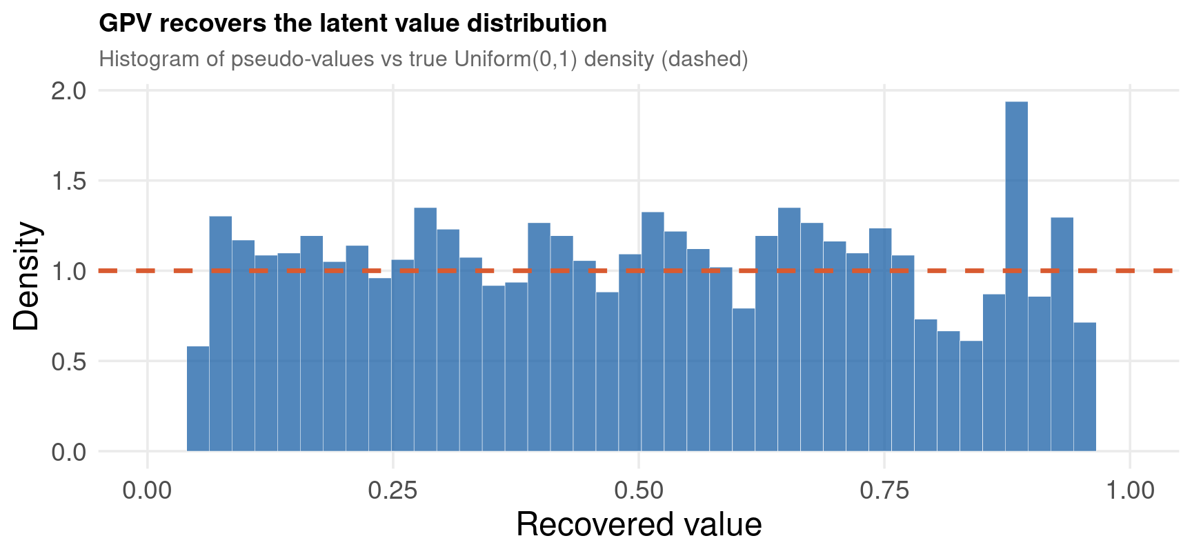
import numpy as np, pandas as pd
import matplotlib.pyplot as plt
from scipy import stats

au = pd.read_csv("../data/structural-auction.csv"); bid = au["bid"].to_numpy(); n = 4
Ghat = np.searchsorted(np.sort(bid), bid, side="right")/len(bid)   # empirical CDF
kde  = stats.gaussian_kde(bid)
vhat = bid + Ghat/((n - 1)*kde(bid))
qlo, qhi = np.quantile(bid, [0.05, 0.95]); keep = (bid > qlo) & (bid < qhi)
print(f"Recovered value mean = {vhat[keep].mean():.3f} (true 0.500), "
      f"sd = {vhat[keep].std():.3f} (true {np.sqrt(1/12):.3f})")
Recovered value mean = 0.500 (true 0.500), sd = 0.264 (true 0.289)(array([1.26992778, 1.21113483, 1.18173836, 1.11706611, 1.14058329,
1.09354893, 1.11118681, 1.14058329, 1.0053595 , 1.18173836,
1.09942822, 1.22877272, 1.08766963, 0.96420443, 1.11118681,
1.08766963, 1.1288247 , 1.05239386, 1.11118681, 1.1229454 ,
1.17585906, 1.05827315, 1.19349695, 0.97596302, 1.15234188,
1.16410047, 1.17585906, 1.21113483, 1.09354893, 1.07591104,
1.02887668, 0.93480795, 0.88777359, 0.85249782, 0.98184231,
1.14646258, 0.95244584, 0.72903262, 0.57617094, 0.51737799]), array([0.05330849, 0.07693188, 0.10055527, 0.12417866, 0.14780206,
0.17142545, 0.19504884, 0.21867223, 0.24229562, 0.26591901,
0.2895424 , 0.31316579, 0.33678918, 0.36041257, 0.38403596,
0.40765935, 0.43128274, 0.45490613, 0.47852952, 0.50215291,
0.5257763 , 0.54939969, 0.57302308, 0.59664648, 0.62026987,
0.64389326, 0.66751665, 0.69114004, 0.71476343, 0.73838682,
0.76201021, 0.7856336 , 0.80925699, 0.83288038, 0.85650377,
0.88012716, 0.90375055, 0.92737394, 0.95099733, 0.97462072,
0.99824411]), <BarContainer object of 40 artists>)<matplotlib.lines.Line2D object at 0x7acdf8f3cd00>(0.0, 1.0)
Text(0.5, 0, 'Recovered value')
Text(0, 0.5, 'Density')Text(0.5, 1.0, 'GPV recovers the latent value distribution')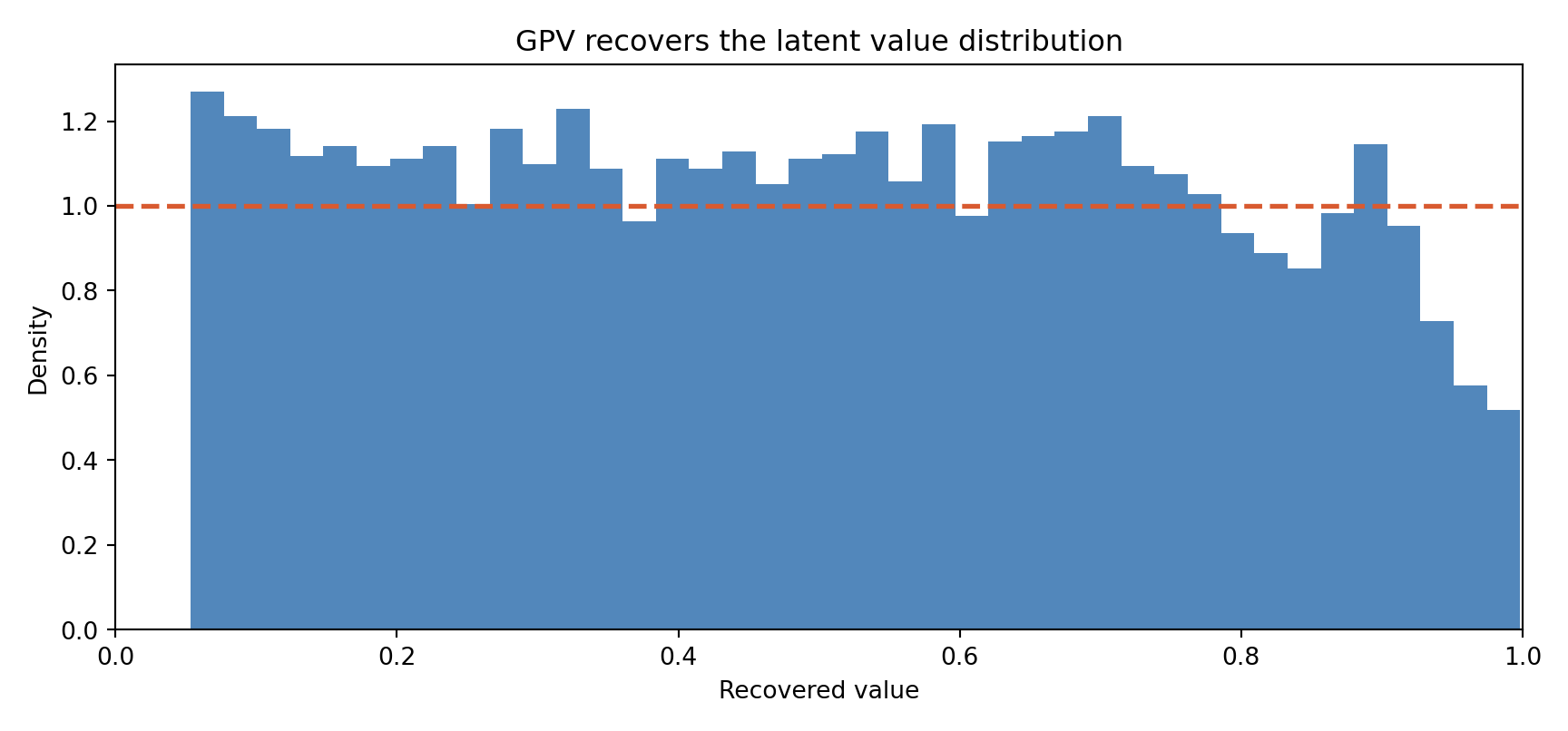
import delimited "../data/structural-auction.csv", clear
quietly destring _all, replace
local n = 4
cumul bid, gen(Ghat)                              // empirical bid CDF
kdensity bid, generate(bx by) at(bid) nograph     // bid density at each bid
gen vhat = bid + Ghat/((`n'-1)*by)                // GPV pseudo-value
summarize vhat if inrange(bid, r(p5), r(p95))
twoway (histogram vhat if inrange(vhat,0,1), density color(navy%60)) ///
       (function y = 1, range(0 1) lcolor(red) lpattern(dash)), ///
  legend(off) xtitle("Recovered value") title("GPV: recovered value distribution")
quietly graph export "../plots/structural-auction-stata.png", replace width(1050) height(650)Burdett & Mortensen (1998): identical firms post wages, identical workers search on and off the job. Frictions (\(\kappa=\lambda/\delta\), the ratio of offer arrival to job destruction) generate a non-degenerate wage distribution even with homogeneous agents — the resolution of the Diamond paradox.
\[ F(w) = \frac{1+\kappa}{\kappa}\left[1 - \sqrt{\frac{p-w}{p-b}}\right],\qquad \bar w = p - \frac{p-b}{(1+\kappa)^2} \]
w <- read.csv("../data/structural-bm.csv")$w      # offers (b = 0, p = 1), from structural-data.R

Fmod <- function(w, k) pmin(pmax((1 + k)/k*(1 - sqrt(pmax(1 - w, 0))), 0), 1)
grid <- as.numeric(quantile(w, seq(0.02, 0.98, 0.02)))
Fhat <- ecdf(w)
kh <- optimize(function(k) sum((Fhat(grid) - Fmod(grid, k))^2), c(0.1, 5))$minimum
cat(sprintf("Burdett-Mortensen : kappa_hat = %.3f   (true 1.500)\n", kh))
Burdett-Mortensen : kappa_hat = 1.450 (true 1.500)wbar <- 1 - 1/(1 + kh)^2
fden <- function(w) (1 + kh)/(2*kh)/sqrt(pmax(1 - w, 1e-6))
ggplot(data.frame(w = w[w < wbar]), aes(w)) +
geom_histogram(aes(y = after_stat(density)), bins = 40,
fill = "#185FA5", alpha = 0.75, color = "white", linewidth = 0.1) +
stat_function(fun = fden, color = "#D85A30", linewidth = 1.2, xlim = c(0, wbar)) +
labs(x = "Wage", y = "Density",
title = "Burdett-Mortensen equilibrium wage density is increasing",
subtitle = "Histogram of offers vs fitted density (red) - the model's signature") +
theme_lecture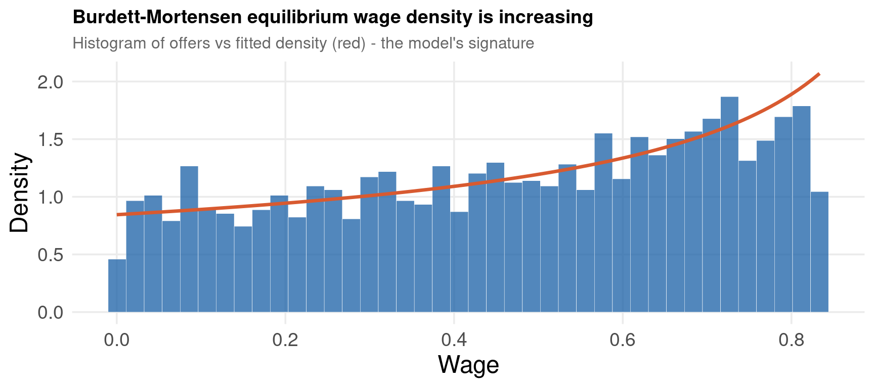
import numpy as np, pandas as pd, matplotlib.pyplot as plt
from scipy import optimize

w = pd.read_csv("../data/structural-bm.csv")["w"].to_numpy()   # from structural-data.R

def Fmod(w, k):
    return np.clip((1 + k)/k*(1 - np.sqrt(np.clip(1 - w, 0, None))), 0, 1)
grid = np.quantile(w, np.arange(0.02, 0.99, 0.02))
Fhat = np.searchsorted(np.sort(w), grid, side="right")/len(w)
kh = optimize.minimize_scalar(lambda k: np.sum((Fhat - Fmod(grid, k))**2),
                              bounds=(0.1, 5), method="bounded").x
print(f"Burdett-Mortensen : kappa_hat = {kh:.3f}   (true 1.500)")
Burdett-Mortensen : kappa_hat = 1.450 (true 1.500)(array([0.86054587, 1.07162316, 0.94172944, 0.87678258, 1.2339903 ,
0.90925601, 0.7793623 , 0.81183573, 0.92549273, 0.90925601,
0.94172944, 1.0066763 , 1.07162316, 0.87678258, 1.1203333 ,
1.18528016, 0.97420287, 0.97420287, 1.2339903 , 0.87678258,
1.20151687, 1.29893716, 1.13657002, 1.15280673, 1.02291301,
1.26646373, 1.16904344, 1.49377773, 1.1203333 , 1.52625116,
1.31517387, 1.52625116, 1.46130431, 1.68861831, 1.81851202,
1.52625116, 1.39635745, 1.75356517, 1.63990817, 1.93216903]), array([5.06774935e-04, 2.13278752e-02, 4.21489755e-02, 6.29700758e-02,
8.37911761e-02, 1.04612276e-01, 1.25433377e-01, 1.46254477e-01,
1.67075577e-01, 1.87896677e-01, 2.08717778e-01, 2.29538878e-01,
2.50359978e-01, 2.71181079e-01, 2.92002179e-01, 3.12823279e-01,
3.33644379e-01, 3.54465480e-01, 3.75286580e-01, 3.96107680e-01,
4.16928781e-01, 4.37749881e-01, 4.58570981e-01, 4.79392081e-01,
5.00213182e-01, 5.21034282e-01, 5.41855382e-01, 5.62676483e-01,
5.83497583e-01, 6.04318683e-01, 6.25139783e-01, 6.45960884e-01,
6.66781984e-01, 6.87603084e-01, 7.08424185e-01, 7.29245285e-01,
7.50066385e-01, 7.70887485e-01, 7.91708586e-01, 8.12529686e-01,
8.33350786e-01]), <BarContainer object of 40 artists>)[<matplotlib.lines.Line2D object at 0x7acdf8ed8b20>]Text(0.5, 0, 'Wage')
Text(0, 0.5, 'Density')Text(0.5, 1.0, 'Burdett-Mortensen equilibrium wage density is increasing')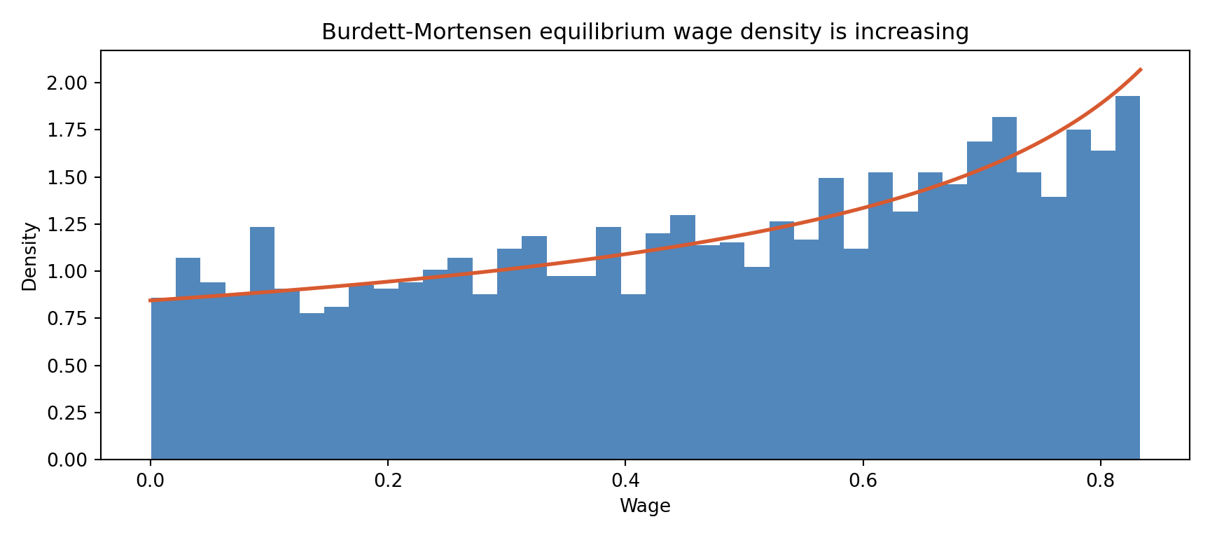
import delimited "../data/structural-bm.csv", clear
quietly destring _all, replace
* Estimate kappa by matching the empirical wage CDF to F(w;kappa). Grid in Mata.
mata:
w = st_data(., "w"); n = rows(w); ws = sort(w, 1)
probs = (1::49):*0.02; np = rows(probs)
grid = J(np,1,0); Fhat = J(np,1,0)
for (i=1; i<=np; i++) {
    idx = ceil(probs[i]*n)
    grid[i] = ws[idx]
    Fhat[i] = mean(w :<= grid[i])          // empirical CDF at grid point
}
kg = rangen(0.1, 5, 500); best = .; khat = .
for (j=1; j<=rows(kg); j++) {
    k = kg[j]
    Fm = (1:+k):/k :* (1 :- sqrt(1 :- grid))    // model CDF F(w;kappa), b=0, p=1
    Fm = rowmin((rowmax((Fm, J(np,1,0))), J(np,1,1)))
    obj = sum((Fhat - Fm):^2)
    if (obj < best) {
        best = obj
        khat = k
    }
}
st_numscalar("khat", khat)
end
local kh = khat
local wbar = 1 - 1/(1+`kh')^2
display "Burdett-Mortensen : kappa_hat = " %5.3f `kh' "   (true 1.500)"
twoway (histogram w if w < `wbar', density color(navy%60)) ///
       (function y = (1+`kh')/(2*`kh')/sqrt(1-x), range(0 `wbar') lcolor(red) lwidth(medthick)), ///
  legend(off) xtitle("Wage") ytitle("Density") ///
  title("Burdett-Mortensen equilibrium wage density is increasing")
quietly graph export "../plots/structural-bm-stata.png", replace width(1050) height(650)
(encoding automatically selected: ISO-8859-2)
(1 var, 3,000 obs)
------------------------------------------------- mata (type end to exit) -----
: w = st_data(., "w"); n = rows(w); ws = sort(w, 1)
: probs = (1::49):*0.02; np = rows(probs)
: grid = J(np,1,0); Fhat = J(np,1,0)
: for (i=1; i<=np; i++) {
> idx = ceil(probs[i]*n)
> grid[i] = ws[idx]
> Fhat[i] = mean(w :<= grid[i]) // empirical CDF at grid point
> }
: kg = rangen(0.1, 5, 500); best = .; khat = .
: for (j=1; j<=rows(kg); j++) {
> k = kg[j]
> Fm = (1:+k):/k :* (1 :- sqrt(1 :- grid)) // model CDF F(w;kappa), b=0,
> p=1
> Fm = rowmin((rowmax((Fm, J(np,1,0))), J(np,1,1)))
> obj = sum((Fhat - Fm):^2)
> if (obj < best) {
> best = obj
> khat = k
> }
> }
: st_numscalar("khat", khat)
: end
-------------------------------------------------------------------------------
Burdett-Mortensen : kappa_hat = 1.445 (true 1.500)
A consumer samples prices sequentially at cost \(c\) per search and buys at the first price below a reservation level \(r\). Optimal \(r\) balances the marginal cost of one more search against its expected saving:
\[ c = \int_{\underline p}^{r} (r-p)\,dG(p) = \int_{\underline p}^{r} G(p)\,dp \]
c_true <- 0.08; r <- sqrt(2*c_true)               # true reservation price = 0.4
price <- read.csv("../data/structural-csearch.csv")$price   # from structural-data.R
rhat <- quantile(price, 0.999)                    # upper support estimates r
chat <- rhat^2/2                                  # invert c = r^2/2
cat(sprintf("Consumer search : r_hat = %.3f (true %.3f),  c_hat = %.4f (true %.4f)\n",
            rhat, r, chat, c_true))
Consumer search : r_hat = 0.399 (true 0.400), c_hat = 0.0798 (true 0.0800)import numpy as np, pandas as pd
c_true = 0.08; r = np.sqrt(2*c_true)
price = pd.read_csv("../data/structural-csearch.csv")["price"].to_numpy() # from structural-data.R
rhat = np.quantile(price, 0.999); chat = rhat**2/2
print(f"Consumer search : r_hat = {rhat:.3f} (true {r:.3f}), c_hat = {chat:.4f} (true {c_true:.4f})")Consumer search : r_hat = 0.399 (true 0.400), c_hat = 0.0798 (true 0.0800)import delimited "../data/structural-csearch.csv", clear
quietly destring _all, replace
* Transaction prices are truncated at the reservation price r: its upper
* support estimates r, then invert c = r^2/2 (uniform prices on [0,1]).
_pctile price, percentiles(99.9)
scalar rhat = r(r1)
scalar chat = rhat^2/2
display "Consumer search : r_hat = " %5.3f rhat " (true 0.400), c_hat = " ///
%6.4f chat " (true 0.0800)"(encoding automatically selected: ISO-8859-2)
(1 var, 4,000 obs)
Consumer search : r_hat = 0.400 (true 0.400), c_hat = 0.0798 (true 0.0800)
Part VI: Partial Identification
When the data pin down a set, not a point
Manski (2003): rather than impose strong assumptions to force point identification, report what the credible weak assumptions alone imply — an identified set.
For \(Y\in[0,1]\) observed only when \(D=1\), the mean is bounded with no assumption on the missing values:
\[ \underbrace{\mathbb E[Y\mid D{=}1]\,\Pr(D{=}1)}_{\text{missing }=0}\ \le\ \mathbb E[Y]\ \le\ \underbrace{\mathbb E[Y\mid D{=}1]\,\Pr(D{=}1) + \Pr(D{=}0)}_{\text{missing }=1} \]
pid <- read.csv("../data/structural-partialid.csv")   # prepared by structural-data.R
yobs <- pid$yobs; d <- pid$d; N <- nrow(pid)

pobs <- mean(d); mo <- mean(yobs[d == 1])
LB <- mo*pobs;  UB <- mo*pobs + (1 - pobs)
# Imbens-Manski 95% CI (expand bounds by one-sided z on each end)
se <- sd(yobs, na.rm = TRUE)/sqrt(N)
CI <- c(LB - 1.645*se, UB + 1.645*se)
cat(sprintf("Identified set for E[Y] : [%.3f, %.3f]   (width = P(missing) = %.3f)\n",
            LB, UB, 1 - pobs))
Identified set for E[Y] : [0.343, 0.644] (width = P(missing) = 0.300)Imbens-Manski 95% CI : [0.337, 0.651] (true 0.500)import numpy as np, pandas as pd
pid = pd.read_csv("../data/structural-partialid.csv")
d = pid["d"].to_numpy(); yobs = pid["yobs"].to_numpy()
pobs = d.mean(); mo = np.nanmean(yobs)
LB = mo*pobs; UB = mo*pobs + (1 - pobs)
se = np.nanstd(yobs, ddof=1)/np.sqrt(len(d))
CI = (LB - 1.645*se, UB + 1.645*se)
print(f"Identified set for E[Y] : [{LB:.3f}, {UB:.3f}] (width = P(missing) = {1-pobs:.3f})")Identified set for E[Y] : [0.343, 0.644] (width = P(missing) = 0.300)Imbens-Manski 95% CI : [0.337, 0.651] (true 0.500)import delimited "../data/structural-partialid.csv", clear
quietly destring _all, replace force
quietly summarize d
scalar pobs = r(mean)
quietly summarize yobs if d == 1
scalar mo = r(mean)
scalar LB = mo*pobs
scalar UB = mo*pobs + (1 - pobs)
display "Identified set for E[Y] : [" %5.3f LB ", " %5.3f UB "] width = " %5.3f (1-pobs)(encoding automatically selected: ISO-8859-2)
(2 vars, 3,000 obs)
Identified set for E[Y] : [0.343, 0.644] width = 0.300Every structural estimator above should be checked by Monte Carlo: re-simulate the DGP many times, re-estimate, and inspect bias and RMSE. Each replication is independent → embarrassingly parallel.
mclapply across 6 cores (see parallel.txt); each worker gets an independent RNG streamlibrary(parallel)
one_rep <- function(rep_id) {
M <- 1500; b0 <- 0.5; b1 <- 1.0; delta <- -1.0
X <- rnorm(M); muM <- b0 + b1*X; muD <- muM + delta
e1 <- rnorm(M); e2 <- rnorm(M)
N <- ifelse(e1 >= -muD & e2 >= -muD, 2L,
ifelse(e1 < -muM & e2 < -muM, 0L, 1L))
negll <- function(par) {
mM <- par[1] + par[2]*X; mD <- mM + par[3]
p2 <- pnorm(mD)^2; p0 <- (1 - pnorm(mM))^2; p1 <- pmax(1 - p2 - p0, 1e-12)
-sum(ifelse(N == 2, log(pmax(p2, 1e-12)),
ifelse(N == 0, log(pmax(p0, 1e-12)), log(p1))))
}
optim(c(0, 0.5, -0.5), negll, method = "BFGS")$par
}
res <- mclapply(1:200, one_rep, mc.cores = 6, mc.set.seed = TRUE)
E <- do.call(rbind, res); colnames(E) <- c("beta0", "beta1", "delta")
tab <- data.frame(true = c(0.5, 1.0, -1.0),
mean = colMeans(E),
bias = colMeans(E) - c(0.5, 1.0, -1.0),
rmse = sqrt(colMeans(sweep(E, 2, c(0.5, 1.0, -1.0))^2)))
print(round(tab, 4)) true mean bias rmse
beta0 0.5 0.5018 0.0018 0.0394
beta1 1.0 0.9967 -0.0033 0.0393
delta -1.0 -0.9998 0.0002 0.0601import numpy as np
from scipy import stats, optimize
Phi = stats.norm.cdf
def one_rep(seed):
rng = np.random.default_rng(seed)
M, b0, b1, delta = 1500, 0.5, 1.0, -1.0
X = rng.standard_normal(M); muM = b0 + b1*X; muD = muM + delta
e1 = rng.standard_normal(M); e2 = rng.standard_normal(M)
N = np.where((e1 >= -muD) & (e2 >= -muD), 2,
np.where((e1 < -muM) & (e2 < -muM), 0, 1))
def negll(par):
mM = par[0] + par[1]*X; mD = mM + par[2]
p2 = Phi(mD)**2; p0 = (1 - Phi(mM))**2; p1 = np.clip(1 - p2 - p0, 1e-12, None)
return -np.sum(np.where(N == 2, np.log(np.clip(p2, 1e-12, None)),
np.where(N == 0, np.log(np.clip(p0, 1e-12, None)), np.log(p1))))
return optimize.minimize(negll, [0, 0.5, -0.5], method="BFGS").x
E = np.array([one_rep(s) for s in range(200)]) # numpy is fast; loop is clear
true = np.array([0.5, 1.0, -1.0])
print("param true mean bias rmse")param true mean bias rmsebeta0 +0.500 +0.501 +0.0013 0.0422
beta1 +1.000 +1.003 +0.0029 0.0433
delta -1.000 -1.006 -0.0063 0.0657Cores
parallel.txt sets N_CORES = 6 on this 8-core machine. In R we pass mc.cores = 6 to mclapply with mc.set.seed = TRUE for independent streams. For the light NumPy loop, vectorised replication is already fast; for heavier estimators use joblib.Parallel(n_jobs=6).
inc as the excluded instrument. Verify recovery of \(\lambda=0.8\) and explain which shifter identifies which equation.inc·cost, which enters demand). Show the J-test now rejects, and interpret.Thank You
Athanassios Stavrakoudis
Applied Informatics and Computational Economics Lab
Department of Economics
University of Ioannina, Greece