Applied Informatics and Computational Economics Lab
9 July 2026
The Synthetic Control Family — A Road Map
εἴδωλον Ἑλένης ἐξέπεμψʼ ἐς Ἴλιον.
he sent a phantom of Helen to Troy
Εὐριπίδης, Ἠλέκτρα 1283
The SC Family at a Glance
One idea runs through the whole lecture: when a single unit (or a few) is treated and you have a panel of untreated donors, build the counterfactual as a weighted combination of donors that tracks the treated unit before treatment, then read the treatment effect off the post-treatment gap.
One treated unit, many pre-periods → ADH SC / SDID / Bayesian SC.
Many treated units, one date → generalized SC / matrix completion.
Many treated units, different dates (staggered) → multisynth / fect / staggered sdid.
Every method returns a gap\(\hat\tau_t = Y^{\text{treated}}_t - \widehat{Y}^{\,0}_t\); the ATT averages it over the post-treatment window.
All examples ship inside installed R packages — no downloads — and are exported to CSV so R, Python and Stata read the same file.
CSV
Source
Role
sc-california.csv
ADH (2010) Prop 99 tobacco
headline real example (1 treated)
sc-germany.csv, sc-basque.csv
ADH (2015), A&G (2003)
secondary real examples
sc-simul.csv
simulated factor panel
known-truth ATT \(=3.75\) (Parts IV–V)
sc-stagger.csv
simulated staggered panel
known-truth ATT \(=4.133\) (Part VI)
Why so many methods?
They differ in how much they let the counterfactual extrapolate and what structure they impose (convex hull vs factors vs low rank). The last Part is a decision framework: which method when.
synth (+ synth_runner) — ADH SC with placebo inference.
sdid — synthetic DiD, incl. staggered adoption.
allsynth — augmented / bias-corrected SC.
Language coverage is uneven — and we say so on every slide
ADH SC, Augmented SC and Synthetic DiD exist in all three languages. Generalized SC and matrix completion are R-first (gsynth/fect); Bayesian SC is R/Python; Proximal SC is Python-only (mlsynth). Where a method is a short, standard computation, we hand-code it in the missing language and check it against the truth or the package — penalized & robust SC, interactive fixed effects, MC-NNM. Where a faithful port would be long or fragile, the tab flags the gap honestly rather than shipping something brittle.
One unit — California — adopts a policy (Proposition 99, a 1989 tobacco tax), and we want the counterfactual: what would per-capita cigarette sales have been without it? With a single treated unit and no randomization, the causal question reduces entirely to estimating one missing outcome path.
sc-california.csv — the Abadie, Diamond & Hainmueller (2010) panel:
39 states × 31 years (1970–2000) of annual per-capita cigarette sales (packs).
California is treated from 1989; the other 38 states form the donor pool.
A long pre-period (1970–1988, 19 years) to pin down the fit.
One “similar” state — arbitrary, and rarely convincing.
Simple average of all states — ignores that some states are far better comparisons than others.
Difference-in-differences — assumes parallel trends the single divergent treated unit often violates.
Regression — extrapolates freely, with no guard against leaning on implausible comparisons.
A data-driven weighted average of donors — a synthetic California — matched on the pre-treatment trajectory and predictors.
Weights are non-negative and sum to one → no extrapolation beyond the donor convex hull.
Sparse and transparent: you can read off which states, and how much, build the counterfactual.
A comparative case study: one aggregate unit (a state, country, firm) is exposed to a policy, and we ask what would have happened without it. The problem — no single control unit looks like California.
Picking one “similar” state is arbitrary and rarely convincing.
A simple average of all states ignores that some are far better comparisons than others.
Synthetic control solves this by choosing a weighted average of donors — a synthetic California — that reproduces California’s pre-treatment trajectory and predictors.
Weights are chosen using only pre-treatment information, so the post-treatment gap is not engineered. The data, not the researcher, pick the comparison unit.
Policy evaluation — a tax, ban, or reform in one jurisdiction (Prop 99 tobacco tax).
Political economy — reunification, conflict, terrorism, institutional change.
Firms & markets — a merger, entry, or product launch in one market.
Any setting with a long pre-period, few treated units, and a pool of untreated donors measured on the same outcome.
Synthetic control is credible only when:
there is a good pre-treatment fit (the synthetic tracks the treated unit);
the treated unit lies inside the convex hull of donors (no extrapolation);
no donor is contaminated by the treatment or by its own large shock;
the pre-period is long enough to rule out a chance fit.
Parts II–III are entirely about diagnosing and defending these conditions.
Units \(i = 1, \dots, N+1\) over periods \(t = 1, \dots, T\). Unit \(1\) is treated from \(T_0+1\) on; units \(2,\dots,N+1\) are the donor pool (never treated). Potential outcomes \(Y_{it}^0\) (no treatment) and \(Y_{it}^1\) (treatment). The observed outcome is
\(Y_{1t}^1 = Y_{1t}\) is observed; the whole problem is the missing counterfactual\(Y_{1t}^0\). Synthetic control estimates it as a weighted average of donor outcomes:
The reported ATT is the post-period average \(\ \widehat{\text{ATT}} = \frac{1}{T-T_0}\sum_{t>T_0}\hat\tau_{1t}.\)
Everything reduces to estimating one counterfactual path. The methods in this lecture differ only in how they build \(\widehat{Y}_{1t}^{\,0}\) — convex weights, factor models, low-rank completion, or a Bayesian time-series model.
DiD forces the counterfactual to move parallel to the controls — a strong restriction the data cannot relax.
Regression with donor outcomes as regressors allows negative weights → the counterfactual can extrapolate outside the donor range.
Synthetic control restricts to convex combinations: no extrapolation, weights are interpretable, and the pre-fit is transparent.
Synthetic DiD (Part VIII) is the bridge
It keeps SC’s data-driven unit weights but also estimates time weights and allows a DiD-style level shift — combining the best of both.
The ADH Weighting Problem — Unit Weights \(W\)
The convex-hull restriction
Non-negative weights that sum to one force the synthetic unit to be a weighted average — it lies inside the convex hull of the donors, never outside their range.
This buys three things: (1) no extrapolation — you cannot manufacture a counterfactual more extreme than any real unit; (2) sparsity — the optimum typically puts weight on only a handful of donors, so the comparison is transparent and interpretable; (3) it makes a poor pre-fit visible — if no convex combination tracks the treated unit, the method warns you rather than hiding it behind extrapolation.
The price: if the treated unit is outside the donor hull (e.g. the most extreme state), no convex combination can match it — a genuine limitation that augmented SC (Part VII) relaxes.
Let \(X_1\) be a \(k\times 1\) vector of pre-treatment characteristics of the treated unit (predictors and/or pre-period outcomes) and \(X_0\) the \(k\times N\) matrix for the donors. Choose the weight vector\(W = (w_2,\dots,w_{N+1})'\) to minimize the predictor discrepancy
The predictor weights \(V\) are not free parameters — ADH choose them to make the resulting \(W(V)\)fit the pre-treatment outcomes best. This is a nested optimization:
\(Z_1, Z_0\) are pre-treatment outcomes (the object we actually want to track).
Inner problem: given \(V\), solve a quadratic program for \(W\).
Outer problem: search over \(V\) to minimize pre-treatment outcome prediction error.
The packages do both loops for you: Synth::synth, pysyncon.Synth, Stata synth.
A common, fully reproducible choice — used for cross-language parity in this deck — is to make every pre-treatment period of the outcome a predictor, so \(X = Z\) and the fit targets the whole pre-path.
\(V\) can also be set by cross-validation or supplied by hand (custom.v).
Parity spec
All three languages here compute SC using all pre-treatment years of cigsale as predictors. That makes the objective identical, so R, Python and Stata return the same weights and the same gap (≈ \(-19\) packs) up to optimizer tolerance.
Synthetic control identifies \(\tau_{1t}\) under (Abadie 2021):
No interference — donors are unaffected by the treatment (SUTVA); a treated-adjacent donor violates this.
Good pre-treatment fit — some \(W\in\Delta\) makes \(Z_0 W \approx Z_1\) over a long pre-period.
Convex-hull / no-extrapolation — the treated unit’s predictors lie (near) inside the donor hull.
No anticipation — behaviour does not change before \(T_0\).
Stable factor structure — donor and treated units are driven by the same latent factors (formalized in Part IV).
Under a linear factor model\(Y_{it}^0 = \delta_t + \lambda_i' f_t + \varepsilon_{it}\), Abadie et al. show that if a \(W\) matches both the pre-period outcomes and the observed predictors, then it also matches the unobserved factor loadings\(\lambda_i\) — so the post-treatment bias vanishes as the number of pre-periods grows.
Bottom line
A long pre-period with a close fit is what makes SC credible — not any single untestable assumption. That is why every applied SC paper leads with the pre-treatment fit plot.
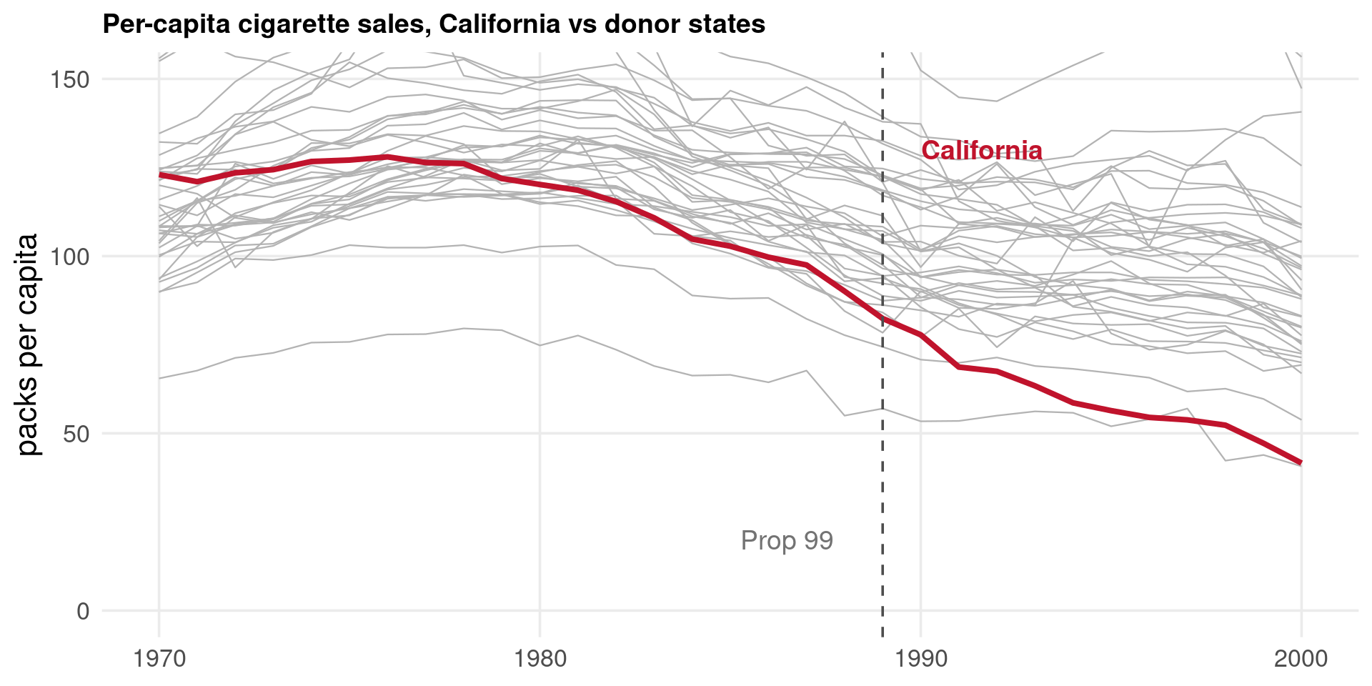
ca <-read.csv("../data/sc-california.csv") # state, year, cigsale, treated# California vs the 38 donor states; treatment (Prop 99) from 1989.ggplot(ca, aes(year, cigsale, group = state)) +geom_line(data =filter(ca, state !="California"),color ="grey70", linewidth =0.4) +geom_line(data =filter(ca, state =="California"),color ="#C0132C", linewidth =1.4) +geom_vline(xintercept =1989, linetype ="dashed", color ="grey30") +annotate("text", x =1989.4, y =40, hjust =0, color ="#C0132C",fontface ="bold", label ="California") +annotate("text", x =1983, y =40, color ="grey45", label ="Prop 99 →") +coord_cartesian(ylim =c(0, 150)) +labs(title ="Per-capita cigarette sales, California vs donor states",x =NULL, y ="packs per capita") +theme(text =element_text(size =16))
Code
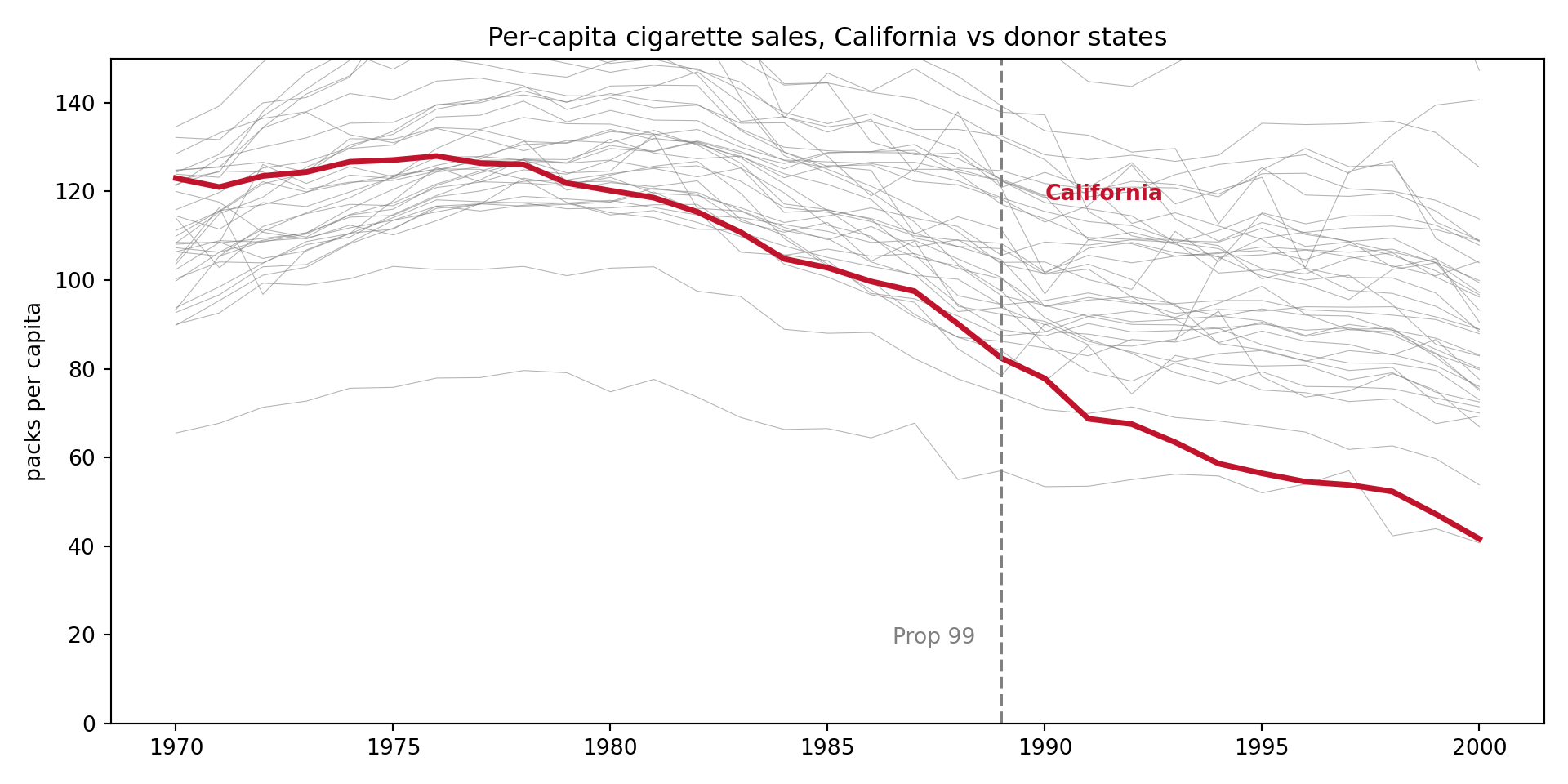
import pandas as pd, matplotlib.pyplot as pltca = pd.read_csv("../data/sc-california.csv")fig, ax = plt.subplots(figsize=(10, 5))for st, g in ca[ca.state !="California"].groupby("state"): ax.plot(g.year, g.cigsale, color="grey", lw=0.4, alpha=0.6)cal = ca[ca.state =="California"]ax.plot(cal.year, cal.cigsale, color="#C0132C", lw=2.6, label="California")ax.axvline(1989, ls="--", color="grey")ax.annotate("California", (1990, 118), color="#C0132C", fontweight="bold")ax.annotate("Prop 99", (1986.5, 18), color="grey")_ = ax.set(ylim=(0, 150), xlabel=None, ylabel="packs per capita", title="Per-capita cigarette sales, California vs donor states")plt.tight_layout(); plt.show()
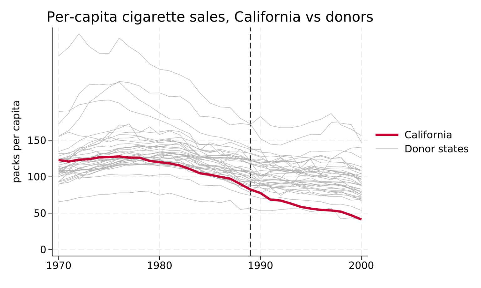
California’s sales sit inside the donor cloud pre-1989 (good — it is in the convex hull) and fall away from it after Prop 99. The raw eye-ball comparison is exactly what SC formalizes: which weighted mix of the grey lines best tracks the red one before 1989?
# tidysynth: SC on ALL pre-treatment outcomes (the cross-language parity spec).sc <- ca %>%synthetic_control(outcome = cigsale, unit = state, time = year,i_unit ="California", i_time =1989,generate_placebos =TRUE)# every pre-treatment year of cigsale becomes a predictorfor (y in1970:1988) sc <- sc %>%generate_predictor(time_window = y, !!paste0("y", y) := cigsale)sc <- sc %>%generate_weights(optimization_window =1970:1988) %>%generate_control()gaps <- sc %>%grab_synthetic_control() # real_y, synth_y by yearatt <-mean((gaps$real_y - gaps$synth_y)[gaps$time_unit >=1989])
Pre-1989 RMSPE : 1.657 packs
Avg post-1989 gap (ATT): -19.49 packs per capita
Code
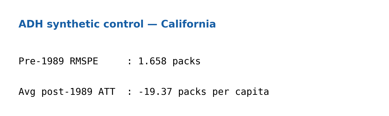
import pandas as pd, numpy as npfrom pysyncon import Dataprep, Synthca = pd.read_csv("../data/sc-california.csv")pre =list(range(1970, 1989))dp = Dataprep( foo=ca, dependent="cigsale", unit_variable="state", time_variable="year", treatment_identifier="California", controls_identifier=[s for s in ca.state.unique() if s !="California"], predictors=[], predictors_op="mean", time_predictors_prior=pre, special_predictors=[("cigsale", [y], "mean") for y in pre], # all pre-outcomes time_optimize_ssr=pre)synth = Synth(); synth.fit(dp)Y = ca.pivot(index="year", columns="state", values="cigsale")w = pd.Series(synth.W, index=dp.controls_identifier)gap = Y["California"] - (Y[w.index] * w.values).sum(axis=1)post = gap.index >=1989rmspe = np.sqrt((gap[~post]**2).mean()); att = gap[post].mean()# knitr+reticulate drops Python stdout after a figure chunk, so the numbers are# drawn on a small results panel (they travel with the figure, which always renders)import matplotlib.pyplot as pltfig, ax = plt.subplots(figsize=(8, 2.4)); ax.axis("off")ax.text(0.03, 0.80, "ADH synthetic control — California", transform=ax.transAxes, fontsize=15, fontweight="bold", color="#185FA5")ax.text(0.03, 0.44, f"Pre-1989 RMSPE : {rmspe:.3f} packs", transform=ax.transAxes, fontsize=14, family="monospace")ax.text(0.03, 0.14, f"Avg post-1989 ATT : {att:.2f} packs per capita", transform=ax.transAxes, fontsize=14, family="monospace")plt.tight_layout(); plt.show()
Code
quietly import delimited "../data/sc-california.csv", clearquietlydestring_all, replaceencode state, gen(id)xtset id yearquietlysummarize id if state=="California", meanonlylocalca = r(mean)* every pre-treatment yearof cigsale is a predictor (the parity spec)local predsforvaluesy = 1970/1988 {local preds `preds' cigsale(`y')}* fit SC and save the treated + synthetic paths to _sc.dta.* synth's plugin floods a long optimizer log that breaks Statamarkdown's* capture; output:false is the only thing that reliably drops it, so the fit* lives here (silent) and the two numbers are reported in the next chunk.synth cigsale `preds', trunit(`ca') trperiod(1989) keep(_sc, replace) nograph
Code
quietlyuse _sc, cleargen gap = _Y_treated - _Y_syntheticgen sq = gap^2 if _time < 1989quietlysummarize sqdisplayastext"Pre-1989 RMSPE : "as result %6.3f sqrt(r(mean)) astext" packs"quietlysummarize gap if _time >= 1989displayastext"Avg post-1989 gap (ATT): "as result %6.2f r(mean) astext" packs per capita"
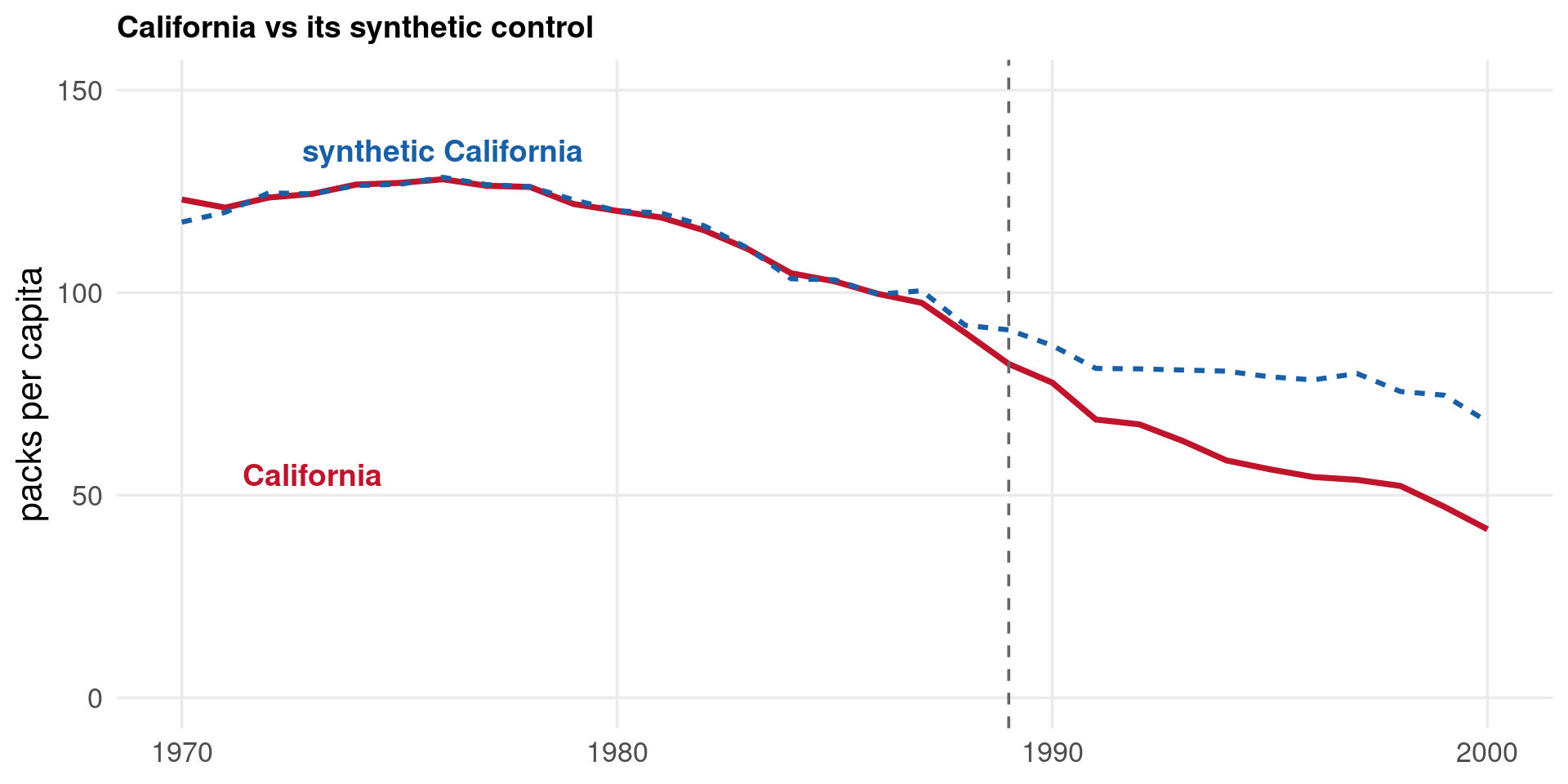
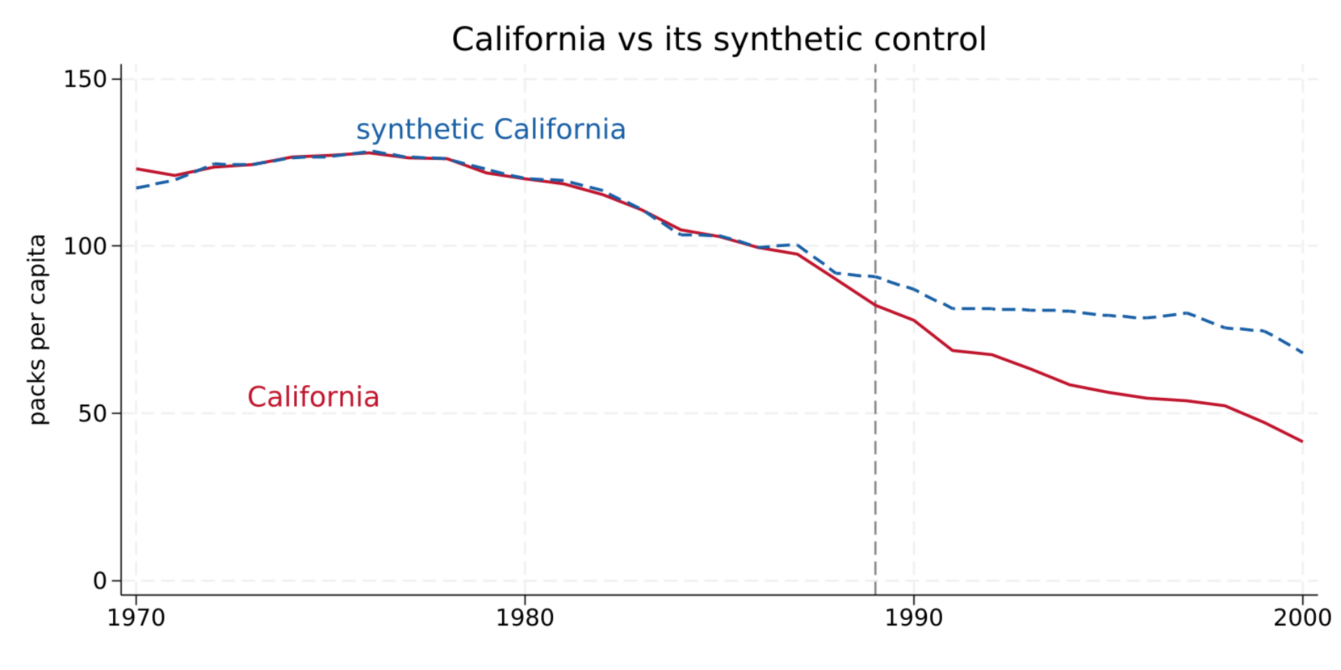
gaps <- sc %>%grab_synthetic_control()ggplot(gaps, aes(time_unit)) +geom_line(aes(y = real_y), color ="#C0132C", linewidth =1.3) +geom_line(aes(y = synth_y), color ="#185FA5", linewidth =1.1, linetype ="22") +geom_vline(xintercept =1989, linetype ="dashed", color ="grey40") +annotate("text", x =1972, y =60, color ="#C0132C", fontface ="bold", label ="California") +annotate("text", x =1972, y =135, color ="#185FA5", fontface ="bold", label ="synthetic California") +coord_cartesian(ylim =c(0, 150)) +labs(title ="California vs its synthetic control", x =NULL, y ="packs per capita") +theme(text =element_text(size =16))
Code
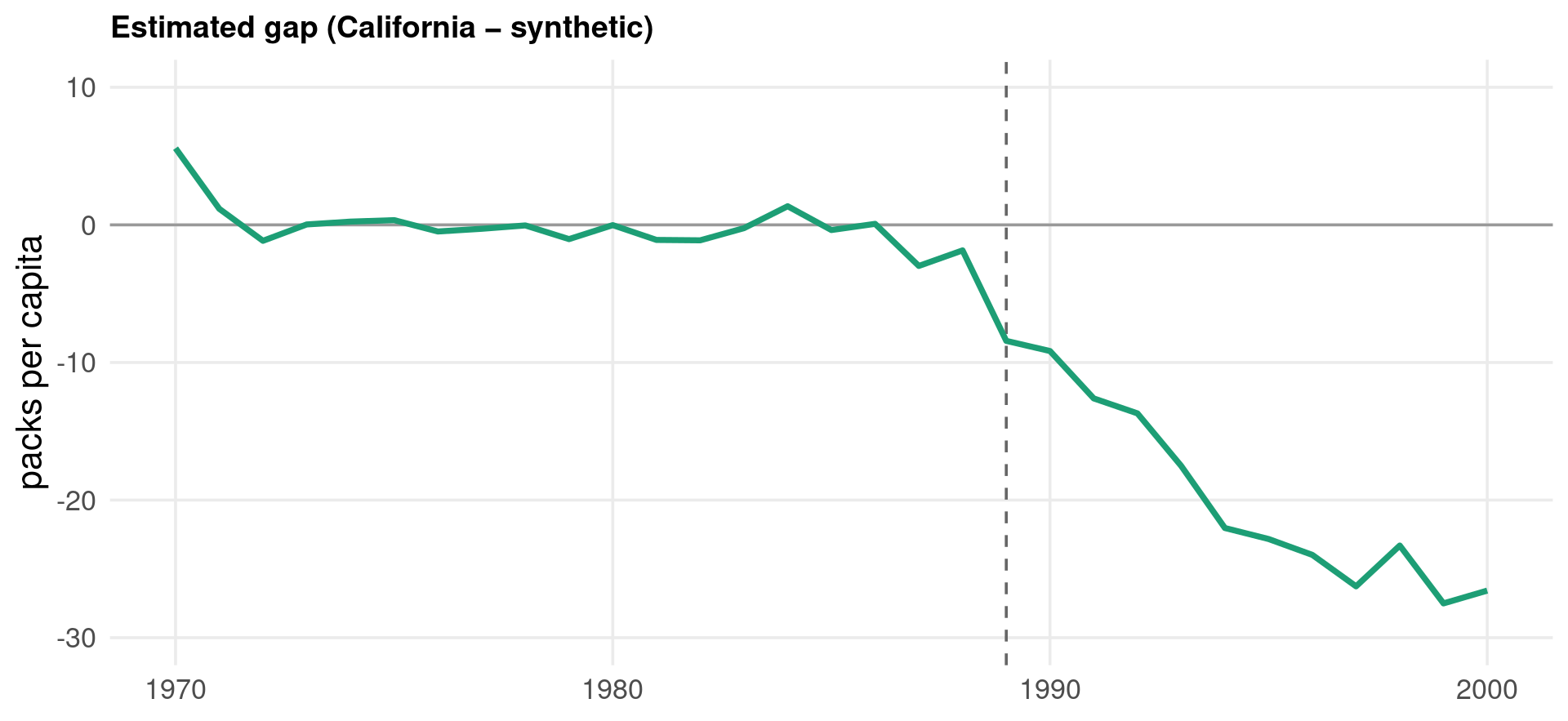
gaps <- sc %>%grab_synthetic_control()gaps$gap <- gaps$real_y - gaps$synth_yggplot(gaps, aes(time_unit, gap)) +geom_hline(yintercept =0, color ="grey60") +geom_vline(xintercept =1989, linetype ="dashed", color ="grey40") +geom_line(color ="#1D9E75", linewidth =1.3) +coord_cartesian(ylim =c(-30, 10)) +labs(title ="Estimated gap (California − synthetic)",x =NULL, y ="packs per capita") +theme(text =element_text(size =16))
The gap hovers around zero before 1989 (good pre-fit) and opens to about −25 packs by 2000 — the growing effect of Prop 99.
Code
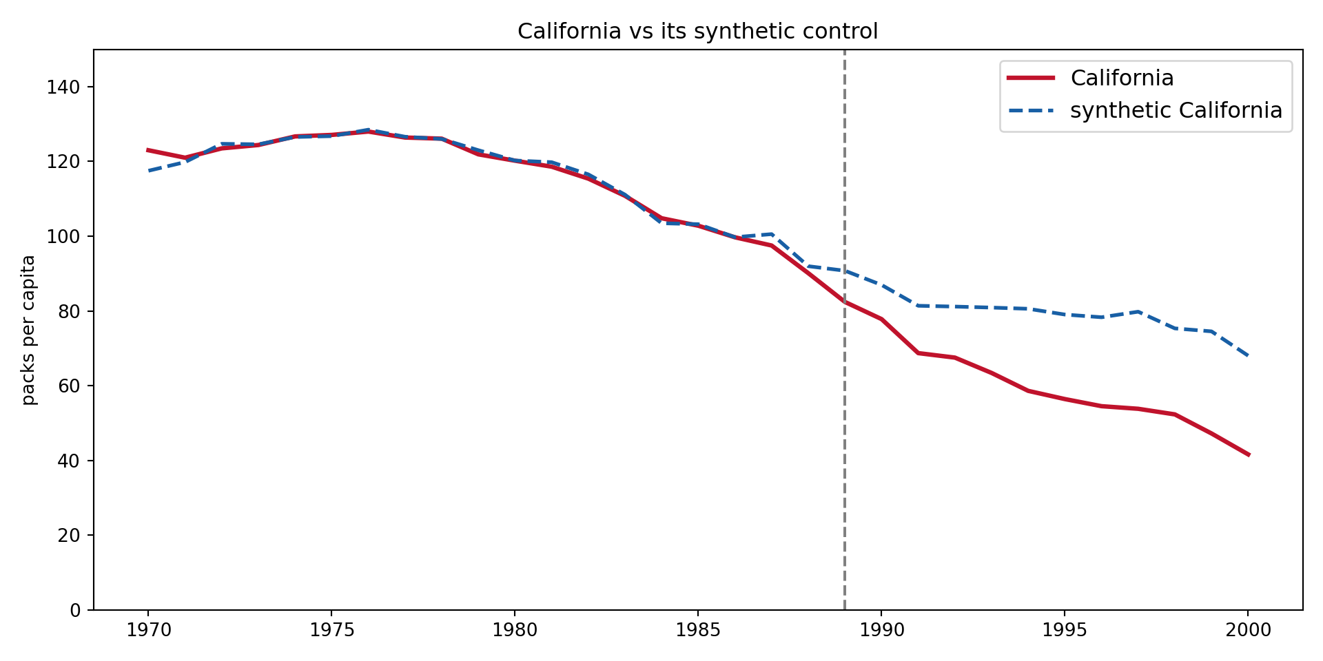
import pandas as pd, matplotlib.pyplot as pltfrom pysyncon import Dataprep, Synthca = pd.read_csv("../data/sc-california.csv"); pre =list(range(1970, 1989))dp = Dataprep( foo=ca, dependent="cigsale", unit_variable="state", time_variable="year", treatment_identifier="California", controls_identifier=[s for s in ca.state.unique() if s !="California"], predictors=[], predictors_op="mean", time_predictors_prior=pre, special_predictors=[("cigsale", [y], "mean") for y in pre], time_optimize_ssr=pre)synth = Synth(); synth.fit(dp)Y = ca.pivot(index="year", columns="state", values="cigsale")w = pd.Series(synth.W, index=dp.controls_identifier)synth_path = (Y[w.index] * w.values).sum(axis=1)fig, ax = plt.subplots(figsize=(10, 5))ax.plot(Y.index, Y["California"], color="#C0132C", lw=2.4, label="California")ax.plot(Y.index, synth_path, color="#185FA5", lw=2.0, ls="--", label="synthetic California")ax.axvline(1989, ls="--", color="grey")_ = ax.set(ylim=(0, 150), ylabel="packs per capita", title="California vs its synthetic control")ax.legend(fontsize=12); plt.tight_layout(); plt.show()
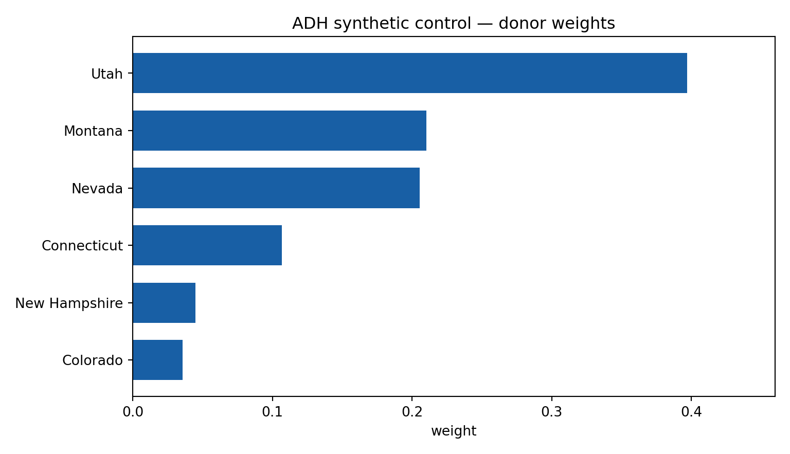
A handful of states — Utah (≈0.40), Montana, Nevada, Connecticut — carry almost all the weight. The synthetic California is a sparse, interpretable mixture, not a black box.
Code
import pandas as pd, matplotlib.pyplot as pltfrom pysyncon import Dataprep, Synthca = pd.read_csv("../data/sc-california.csv"); pre =list(range(1970, 1989))dp = Dataprep( foo=ca, dependent="cigsale", unit_variable="state", time_variable="year", treatment_identifier="California", controls_identifier=[s for s in ca.state.unique() if s !="California"], predictors=[], predictors_op="mean", time_predictors_prior=pre, special_predictors=[("cigsale", [y], "mean") for y in pre], time_optimize_ssr=pre)synth = Synth(); synth.fit(dp)w = pd.Series(synth.W, index=dp.controls_identifier)top = w[w >0.001].sort_values()fig, ax = plt.subplots(figsize=(8, 4.6))ax.barh(top.index, top.values, color="#185FA5", height=0.7)_ = ax.set(xlim=(0, 0.46), xlabel="weight", title="ADH synthetic control — donor weights")plt.tight_layout(); plt.show()
Synthetic control matches the treated unit’s pre-treatment predictors, not just the outcome. Reporting a balance table (treated vs synthetic vs donor-pool average) is standard practice — the synthetic column should sit far closer to the treated unit than the raw donor average, evidence that the weights, not luck, drive the fit.
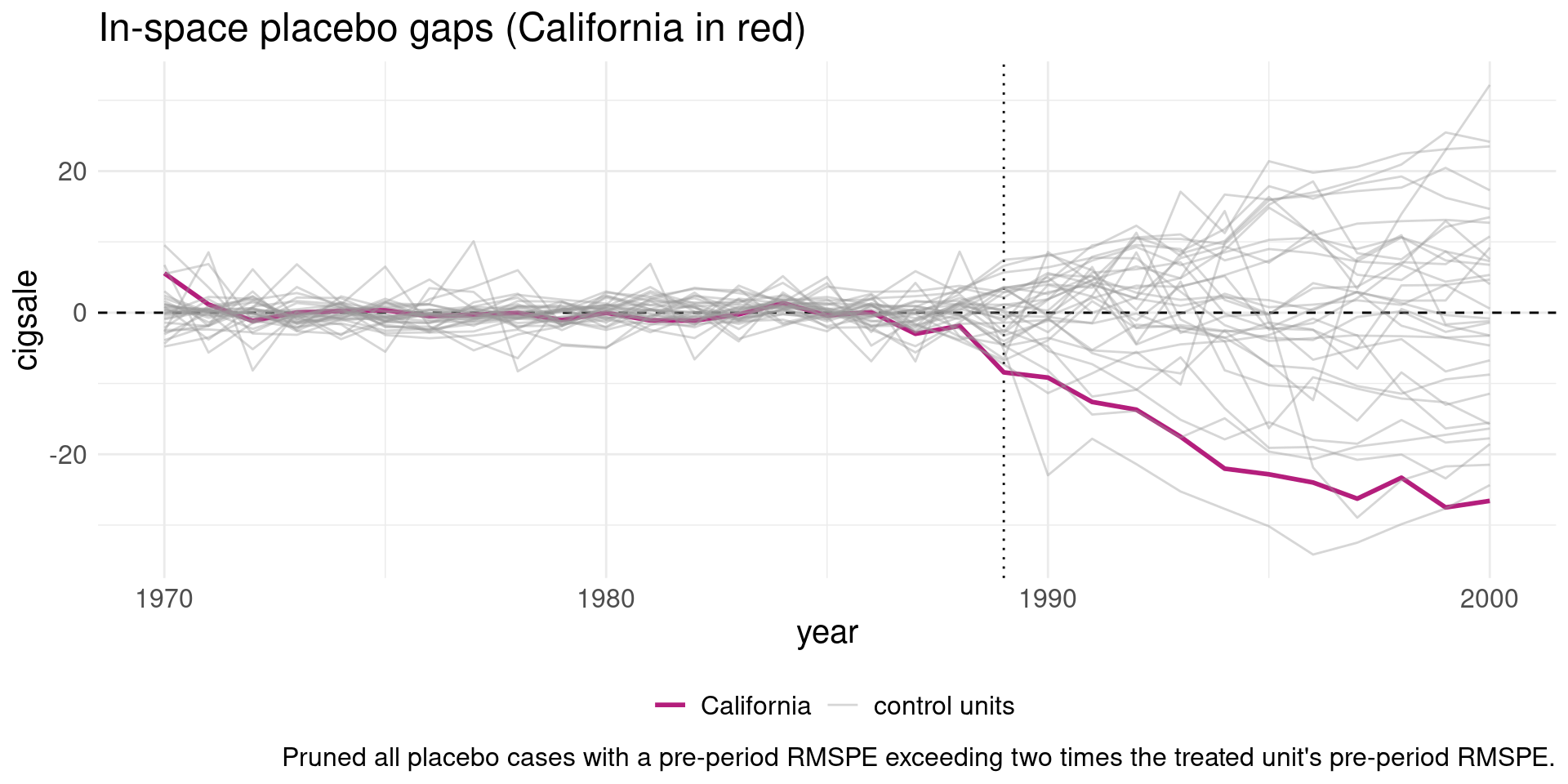
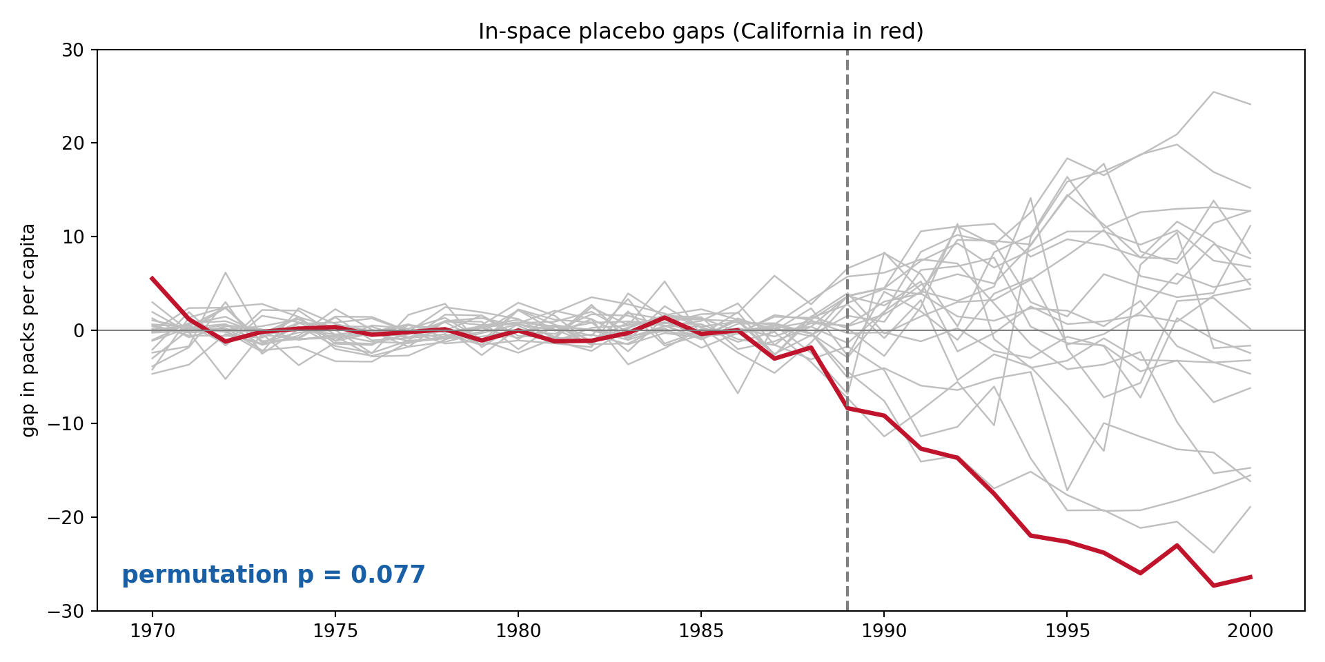
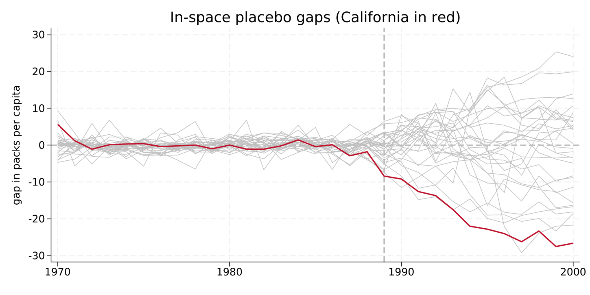
There is one treated unit, so classical standard errors do not apply. ADH inference is a permutation test: pretend each donor was treated in 1989, compute its placebo gap, and ask whether California’s gap is extreme relative to the placebo distribution.
If California’s post/pre RMSPE ratio is the largest among \(N+1\) units, the one-sided \(p\)-value is \(1/(N+1)\).
Placebos with a poor pre-fit are usually discarded (they can produce huge gaps for the wrong reason).
Code
# tidysynth built the placebos already (generate_placebos = TRUE).sc %>%plot_placebos(prune =TRUE) # all placebo gaps, California highlightedsc %>%grab_significance() # RMSPE ratios + permutation p-value
Unit
Post/Pre MSPE ratio
Permutation p-value
California
74
0.0769231
With the pre-outcome-only parity spec, California’s post/pre MSPE ratio is among the most extreme (rank 3 of 39, permutation \(p \approx 0.08\)). Under ADH’s original predictor set (income, price, beer, age + three lagged outcomes) plus placebo pruning, California is the single most extreme unit (\(p \approx 1/39 \approx 0.026\)) — a reminder that SC inference is sensitive to the predictor specification.
Code
import pandas as pd, matplotlib.pyplot as pltfrom pysyncon import Dataprep, Synthca = pd.read_csv("../data/sc-california.csv"); pre =list(range(1970, 1989))states =list(ca.state.unique())Y = ca.pivot(index="year", columns="state", values="cigsale")# fit one SC per unit (pretend each was treated in 1989) and return its gapdef sc_gap(treated, donors): dp = Dataprep( foo=ca, dependent="cigsale", unit_variable="state", time_variable="year", treatment_identifier=treated, controls_identifier=donors, predictors=[], predictors_op="mean", time_predictors_prior=pre, special_predictors=[("cigsale", [y], "mean") for y in pre], time_optimize_ssr=pre) s = Synth(); s.fit(dp) w = pd.Series(s.W, index=donors)return Y[treated] - (Y[w.index] * w.values).sum(axis=1)gaps = pd.DataFrame({u: sc_gap(u, [s for s in states if s != u]) for u in states})treated = gaps["California"]pre_mspe = gaps.loc[:1988].pow(2).mean()post_mspe = gaps.loc[1989:].pow(2).mean()# ADH / Fisher permutation p-value: rank California's post/pre RMSPE ratioratio = post_mspe / pre_mspep = (ratio >= ratio["California"]).sum() /len(ratio)# prune donors whose pre-1989 fit is far worse than California's, as tidysynth doeskeep = pre_mspe[pre_mspe <=2* pre_mspe["California"]].indexfig, ax = plt.subplots(figsize=(10, 5))for u in keep:if u !="California": ax.plot(gaps.index, gaps[u], color="#BFBFBF", lw=0.9)ax.plot(treated.index, treated.values, color="#C0132C", lw=2.4)ax.axhline(0, color="grey", lw=0.8)ax.axvline(1989, ls="--", color="grey")# annotate the p-value ON the figure — the reticulate/knitr text-capture bug# silently drops stdout from a Python chunk that also emits a figure, so the# number is drawn on the axes rather than printed.ax.text(0.02, 0.05, f"permutation p = {p:.3f}", transform=ax.transAxes, fontsize=13, color="#185FA5", fontweight="bold")_ = ax.set(ylim=(-30, 30), xlabel=None, ylabel="gap in packs per capita", title="In-space placebo gaps (California in red)")plt.tight_layout(); plt.show()
Code
quietly import delimited "../data/sc-california.csv", clearquietlydestring_all, replaceencode state, gen(id)xtset id yearquietlysummarize id if state=="California", meanonlylocalca = r(mean)local predsforvaluesy = 1970/1988 {local preds `preds' cigsale(`y')}* synth_runner fits SC for California and for every donor as a placebo;* gen_vars adds effect (the gap) and pre_rmspe for each unit. It floods a long* optimizer log that breaks Statamarkdown, so the fit runs output:false.setseed 14159synth_runner cigsale `preds', trunit(`ca') trperiod(1989) gen_vars* keep placebos whose pre-1989 fit is not far worse than California'squietlysummarize pre_rmspe if id==`ca', meanonlylocal caprmspe = r(mean)sort id yeartwoway (line effect yearif id!=`ca' & pre_rmspe<=2*`caprmspe', ///connect(L) lcolor(gs12) lwidth(thin)) /// (line effect yearif id==`ca', ///connect(L) lcolor("192 19 44") lwidth(medthick)), ///yline(0, lcolor(gs10)) xline(1989, lpattern(dash) lcolor(gs8)) ///yscale(range(-30 30)) ylabel(-30(10)30, angle(0)) ///ytitle("gap in packs per capita") xtitle("") ///title("In-space placebo gaps (California in red)") ///legend(off) graphregion(color(white)) plotregion(color(white)) ///xsize(10) ysize(5)graphexport"../plots/placebo-stata.png", replacewidth(1600)
Read the ratio, not the raw gap
A donor with a lousy pre-fit can post a bigger post-gap than California by chance. The post/pre RMSPE ratio normalizes for pre-fit, so only units the method could actually track compete with California.
Move the “treatment” to a fake earlier date (e.g. 1980) when nothing happened. A credible design shows no gap at the placebo date: the synthetic keeps tracking California through 1980–1988 and only diverges at the true 1989 cut-off.
A spurious jump at the fake date would signal an overfit or an unstable donor pool.
Re-estimate the SC dropping one high-weight donor at a time. If the conclusion survives removing Utah, Nevada, etc., the result is not an artefact of a single donor. (We return to this in Part II.)
A defensible SC paper reports all four:
the path + gap plot;
in-space placebos with the RMSPE-ratio \(p\)-value;
Predictor set (\(V\)) drives the result — pre-outcomes-only vs the ADH covariate set moves the placebo \(p\)-value from \(\approx 0.08\) to \(\approx 0.03\).
Donor pool — exclude contaminated or dissimilar states; bigger is not better.
Placebo pruning — drop donors whose pre-fit is far worse than the treated unit’s (e.g. RMSPE \(> 2\times\)).
Part II — Practical Issues & SC Variants
λόχων, προκρίνας οἵπερ ἀλκιμώτατοι.
of the companies, picking out those who are strongest
Plain ADH synthetic control can break: a poor pre-fit, weights piled on dissimilar or noisy donors, non-unique solutions, or a treated unit outside the donor hull. Part II is about diagnosing these failures and repairing them.
Same California Prop 99 panel (sc-california.csv) — we reuse the 39-state, 1970–2000 series to stress-test donor-pool choice, extrapolation, and the penalized / robust variants against the familiar ADH benchmark.
Weights can be non-unique — many donor mixes fit the pre-period equally well.
Interpolation bias — averaging individually dissimilar donors that only match in aggregate.
Measurement noise in the donor matrix corrupts the weights.
An outlier treated unit lies beyond the convex hull → poor fit by construction.
Penalized SC — a penalty rewarding individually close donors → unique, sparse weights.
Robust SC — SVD de-noising of the donor matrix before fitting.
Leave-one-out and a failure checklist to defend (or retract) an estimate.
The donor pool is a modelling choice, not an afterthought. Include only units that:
share the treated unit’s structural data-generating process (same factors);
are not themselves treated or affected by the intervention (no interference);
did not experience their own large idiosyncratic shock in the window;
are comparable in scale (do not let one giant unit dominate).
In California Prop 99, ADH dropped states that adopted their own large tobacco-control programmes (Massachusetts, Arizona, Oregon, Florida, DC, Alaska, Hawaii) — they would contaminate the counterfactual.
This leaves the 38 “clean” donors in sc-california.csv.
Bigger is not better
Adding irrelevant donors enlarges the convex hull and invites overfitting the pre-period through spurious combinations. A small, defensible pool beats a kitchen-sink pool. Report the pool and justify every inclusion/exclusion.
Convex weights place the synthetic unit inside the convex hull of the donors. Two consequences:
If the treated unit is interior, a good fit is possible with no extrapolation.
If the treated unit is on or beyond the boundary (an extreme outlier), no convex combination can reach it — the pre-fit is poor by construction, and SC will bias toward the interior.
\[Y_1^{\text{pre}} \in \text{conv}\{Y_2^{\text{pre}}, \dots, Y_{N+1}^{\text{pre}}\}\ \Longleftrightarrow\ \text{SC can fit without extrapolating.}\]
Regression / IFE allow negative weights → can always “fit” the treated unit, but by extrapolating — dangerous.
SC refuses to extrapolate → safer, but fails visibly for outliers.
Augmented SC (Part VII) is the principled middle: SC first, then a small model-based extrapolation correction, penalized so it stays close to convex.
A large pre-treatment RMSPE, or weights piled on the most extreme donors, is the signature of an extrapolation problem. That is when you reach for augmented SC or a larger/better pool.
Even inside the hull, SC can suffer interpolation bias: matching the treated unit with donors that are individually very different but average out. If those donors respond differently to shocks, the synthetic diverges post-treatment for the wrong reason.
Guard: prefer weights on donors that are individually similar to the treated unit, not just similar in aggregate.
Guard: demand a long pre-period with a close fit — the more pre-periods matched, the less room for a coincidental fit.
The universal fit statistic is the pre-treatment RMSPE:
Plain SC weights are not unique when many donor combinations fit the pre-period equally well — and it may spread weight across dissimilar donors, inviting interpolation bias. Abadie & L’Hour add a penalty that rewards using donors individually close to the treated unit:
\(\lambda = 0\) → ordinary SC. Large \(\lambda\) → a pure matching estimator (nearest donor).
The penalty makes \(W\)unique and sparse, favouring good bilateral matches.
Designed for disaggregated data (many units) where plain SC is unstable.
Trades a little pre-fit for robustness and interpretability of the comparison set.
Tooling
Available in Python via pysyncon.PenalizedSynth. There is no packaged CRAN/Stata command, but the estimator is a small convex quadratic program on the simplex, so we hand-code it in R with quadprog — it matches pysyncon to the decimal. Stata has no built-in simplex QP solver, so we flag it as a genuine coverage gap rather than write a fragile custom optimizer.
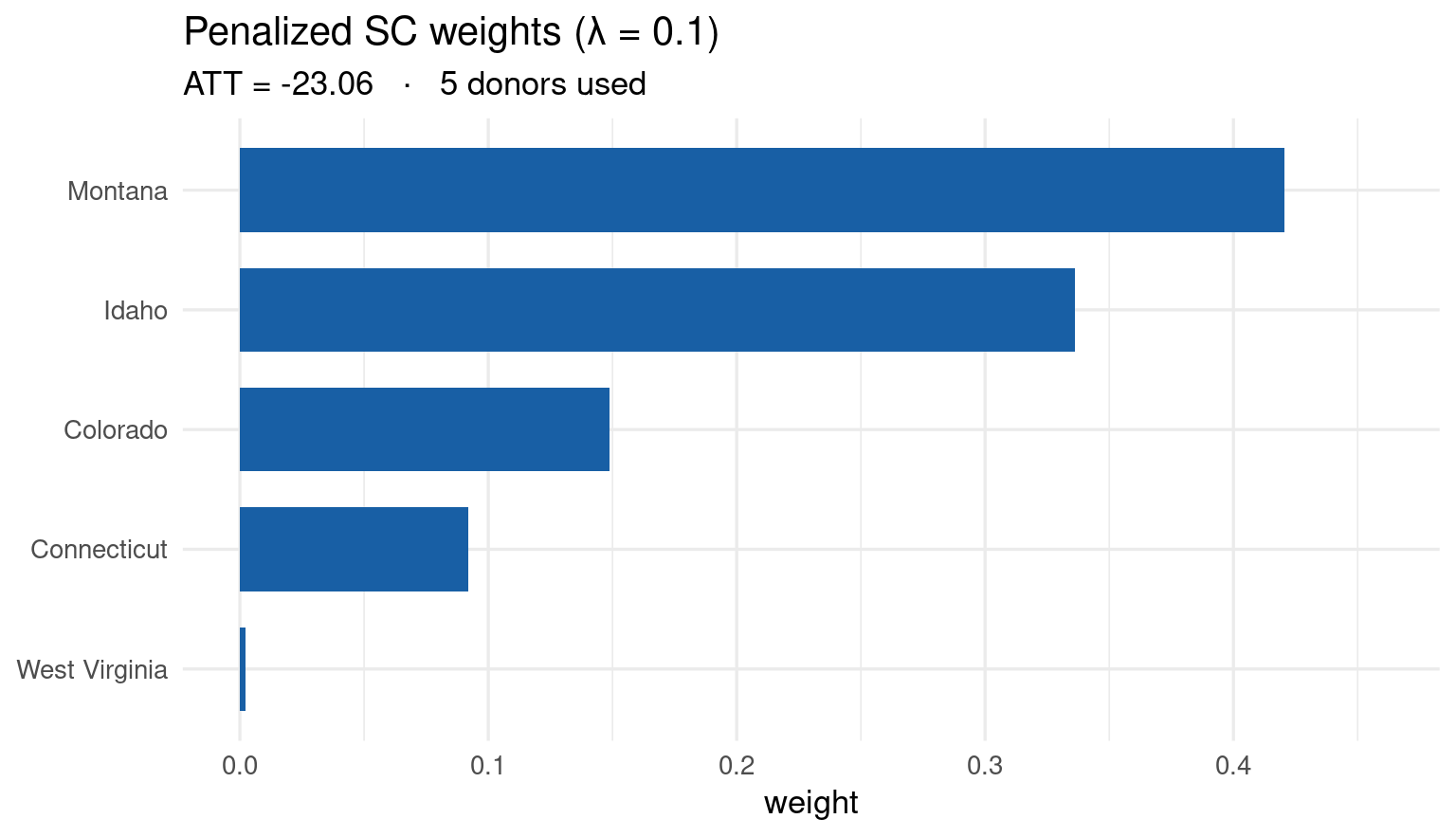
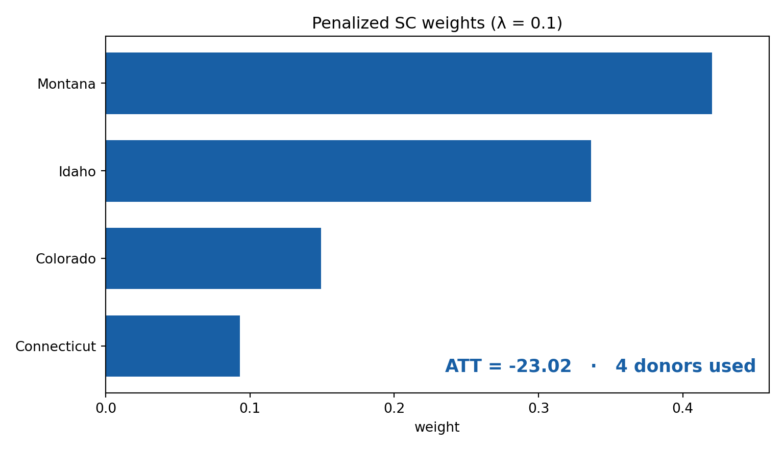
import pandas as pd, numpy as np, matplotlib.pyplot as pltfrom pysyncon import Dataprep, PenalizedSynthca = pd.read_csv("../data/sc-california.csv"); pre =list(range(1970, 1989))don = [s for s in ca.state.unique() if s !="California"]dp = Dataprep( foo=ca, dependent="cigsale", unit_variable="state", time_variable="year", treatment_identifier="California", controls_identifier=don, predictors=[], predictors_op="mean", time_predictors_prior=pre, special_predictors=[("cigsale", [y], "mean") for y in pre], time_optimize_ssr=pre)pen = PenalizedSynth(); pen.fit(dp, lambda_=0.1) # lambda_ = penalty strengthY = ca.pivot(index="year", columns="state", values="cigsale"); post = Y.index >=1989w = pd.Series(pen.W, index=don)att = (Y["California"] - (Y[w.index] * w.values).sum(axis=1))[post].mean()top = w[w >0.001].sort_values()fig, ax = plt.subplots(figsize=(8, 4.6))ax.barh(top.index, top.values, color="#185FA5", height=0.7)ax.text(0.98, 0.06, f"ATT = {att:.2f} · {(w >0.001).sum()} donors used", transform=ax.transAxes, ha="right", fontsize=13, color="#185FA5", fontweight="bold")_ = ax.set(xlim=(0, 0.46), xlabel="weight", title="Penalized SC weights (λ = 0.1)")plt.tight_layout(); plt.show()
No Stata command for penalized SC. Use plain synth (\(\lambda=0\)) and move to Python for the penalty — a genuine coverage gap, not an omission on our part.
Reading the output
The penalty concentrates weight on fewer, better-matched donors than plain SC and yields a slightly larger ATT (≈ −23), a sign it is leaning on closer bilateral matches rather than a broad interpolation.
Measurement noise and missing entries corrupt the donor matrix. Robust SC first de-noises it: take the donor outcome matrix, compute its singular value decomposition, keep only the top few singular values (a low-rank approximation), then fit SC weights on the cleaned matrix by (unconstrained) linear regression.
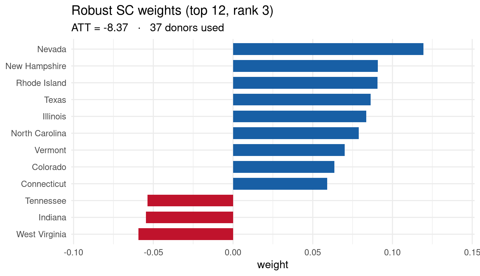
library(ggplot2)ca <-read.csv("../data/sc-california.csv"); pre <-1970:1988don <-setdiff(unique(ca$state), "California")W <- ca %>%select(state, year, cigsale) %>%pivot_wider(names_from = state, values_from = cigsale) %>%as.data.frame()rownames(W) <- W$year; W$year <-NULLYd <-as.matrix(W[, don]); post <-as.numeric(rownames(W)) >=1989; n <-length(don)# de-noise the donor matrix: keep the top 3 singular valuessv <-svd(t(Yd)); k <-3M <-t(sv$u[, 1:k] %*%diag(sv$d[1:k]) %*%t(sv$v[, 1:k])) # cleaned, time x donors# ridge-regress treated pre-period on the cleaned donors (no simplex constraint)Mpre <- M[as.numeric(rownames(W)) <1989, ]X1 <- W[as.character(pre), "California"]w <-as.numeric(solve(t(Mpre) %*% Mpre +0.1*diag(n), t(Mpre) %*% X1))names(w) <- donatt <-mean((W[, "California"] - Yd %*% w)[post])top <-order(-abs(w))[1:12]; d <-data.frame(donor = don[top], w = w[top])ggplot(d, aes(reorder(donor, w), w, fill = w >0)) +geom_col(width =0.7) +coord_flip() +scale_fill_manual(values =c(`TRUE`="#185FA5", `FALSE`="#C0132C"), guide ="none") +scale_y_continuous(limits =c(-0.09, 0.14)) +labs(x =NULL, y ="weight", title ="Robust SC weights (top 12, rank 3)",subtitle =sprintf("ATT = %.2f · %d donors used", att, sum(abs(w) >0.001))) +theme_minimal(base_size =13)
Code
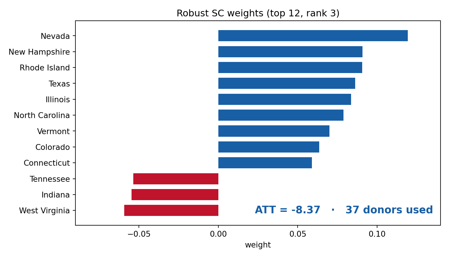
import pandas as pd, numpy as np, matplotlib.pyplot as pltfrom pysyncon import Dataprep, RobustSynthca = pd.read_csv("../data/sc-california.csv"); pre =list(range(1970, 1989))don = [s for s in ca.state.unique() if s !="California"]dp = Dataprep( foo=ca, dependent="cigsale", unit_variable="state", time_variable="year", treatment_identifier="California", controls_identifier=don, predictors=[], predictors_op="mean", time_predictors_prior=pre, special_predictors=[("cigsale", [y], "mean") for y in pre], time_optimize_ssr=pre)Y = ca.pivot(index="year", columns="state", values="cigsale"); post = Y.index >=1989rob = RobustSynth()rob.fit(dp, lambda_=0.1, sv_count=3) # keep top 3 singular values (de-noise)w = pd.Series(rob.W, index=don)att = (Y["California"] - (Y[w.index] * w.values).sum(axis=1))[post].mean()top = w.reindex(w.abs().sort_values(ascending=False).index[:12]).sort_values()cols = ["#185FA5"if v >0else"#C0132C"for v in top.values]fig, ax = plt.subplots(figsize=(8, 4.6))ax.barh(top.index, top.values, color=cols, height=0.7)ax.text(0.98, 0.06, f"ATT = {att:.2f} · {(w.abs() >0.001).sum()} donors used", transform=ax.transAxes, ha="right", fontsize=13, color="#185FA5", fontweight="bold")_ = ax.set(xlim=(-0.09, 0.14), xlabel="weight", title="Robust SC weights (top 12, rank 3)")plt.tight_layout(); plt.show()
Code
quietly import delimited "../data/sc-california.csv", clearquietlykeep state year cigsalequietlyreplace state = subinstr(state, " ", "", .)quietlyreshapewide cigsale, i(year) j(state) stringquietlyds cigsale*local don `r(varlist)'local don : subinstrlocal don "cigsaleCalifornia""", wordmata:years = st_data(., "year")Yd = st_data(., tokens(st_local("don"))) // time x donorsu=.; s=.; v=.svd(Yd', u, s, v) // de-noise the donor matrixs[|4 \ rows(s)|] = J(rows(s) - 3, 1, 0) // keep the top 3 singular valuesM = ((u :* s') * v)' // cleaned, time x donorsnpre = sum(years :< 1989)Mpre = M[|1,1 \ npre,.|]y1 = st_data(., "cigsaleCalifornia")w = luinv(Mpre'Mpre + 0.1*I(cols(Mpre))) * Mpre'y1[|1 \ npre|] // ridge fitatt = mean(select(y1 - Yd*w, years :>= 1989))printf("Robust SC (rank 3): ATT = %6.3f, donors used = %g\n", att, sum(abs(w):>0.001))end
------------------------------------------------- mata (type end to exit) ----------------------------------------------
: years = st_data(., "year")

: Yd    = st_data(., tokens(st_local("don")))     // time x donors

: u=.; s=.; v=.

: svd(Yd', u, s, v)                                // de-noise the donor matrix

: s[|4 \ rows(s)|] = J(rows(s) - 3, 1, 0)          // keep the top 3 singular values

: M     = ((u :* s') * v)'                          // cleaned, time x donors

: npre  = sum(years :< 1989)

: Mpre  = M[|1,1 \ npre,.|]

: y1    = st_data(., "cigsaleCalifornia")

: w     = luinv(Mpre'Mpre + 0.1*I(cols(Mpre))) * Mpre'y1[|1 \ npre|]   // ridge fit

: att   = mean(select(y1 - Yd*w, years :>= 1989))

: printf("Robust SC (rank 3): ATT = %6.3f,  donors used = %g\n", att, sum(abs(w):>0.001))
Robust SC (rank 3): ATT = -8.373,  donors used = 37

: end
------------------------------------------------------------------------------------------------------------------------
The mlsynth package offers a whole family of de-noised / robust SC estimators (RSC, CLUSTERSC, SNN, PCASC, …) under a common API — useful when you want to compare several robustness strategies at once.
Interpretation
De-noising spreads weight across many more donors (≈ 37 here) and returns a more conservative ATT (≈ −8): it trusts the low-rank signal rather than any single donor, at the cost of SC’s sparse interpretability.
Re-estimate the SC dropping each high-weight donor in turn. Overlay the resulting counterfactual paths: if the estimated effect is stable across all leave-one-out fits, no single donor drives it.
Code
# Drop each donor with weight > 5%, refit, collect the post-period ATT.key <- (sc %>%grab_unit_weights() %>% dplyr::filter(weight >0.05))$unitloo <-numeric(length(key)); names(loo) <- keyfor (drop in key) { d <-filter(ca, state != drop) f <- d %>%synthetic_control(cigsale, state, year, "California", 1989, generate_placebos =FALSE)for (y in1970:1988) f <- f %>%generate_predictor(time_window = y, !!paste0("y", y) := cigsale) f <- f %>%generate_weights(optimization_window =1970:1988) %>%generate_control() g <- f %>%grab_synthetic_control() loo[drop] <-mean((g$real_y - g$synth_y)[g$time_unit >=1989])}
Donor dropped
ATT
Connecticut
-20.50
Montana
-17.96
Nevada
-19.20
Utah
-19.08
— none (full) —
-19.49
The ATT stays around −19 to −20 whichever single top donor is removed — the result is not an artefact of Utah or any one state.
A stable table = robust design.
A wild swing when one donor is dropped = the effect hinges on that donor; investigate why (is it contaminated? an outlier?).
Poor pre-fit — large pre-RMSPE relative to the outcome scale.
Extrapolation — treated unit outside the donor hull; weights piled on extremes.
Short pre-period — too few periods to rule out a coincidental fit.
Contaminated donors — a donor treated/shocked in the window (interference).
Fragile weights — leave-one-out swings the conclusion.
In-time placebo fails — a gap appears at a fake pre-treatment date.
Anticipation — behaviour changes before \(T_0\) (bury \(T_0\) earlier).
Each failure has a fix in this lecture: augmented SC (extrapolation), penalized/robust SC (fragile weights, noise), generalized SC / matrix completion (many units, factor confounding), synthetic DiD (imperfect pre-fit), and the sensitivity tools of Part III.
With one treated unit and no randomization, classical standard errors do not apply. How do we attach honest uncertainty to a synthetic-control estimate?
Same California Prop 99 panel — inference is layered on top of the Part I fit, so the donor pool, predictors, and pre/post split carry over unchanged.
N = 1 treated unit — no repeated sampling to form a sampling distribution.
Large-sample asymptotics simply do not hold.
A single point estimate with a star overstates how much we know.
Permutation / placebo tests — the placebo distribution is the null.
Firpo–Possebom design-based confidence sets — invert a randomization test over an effect grid.
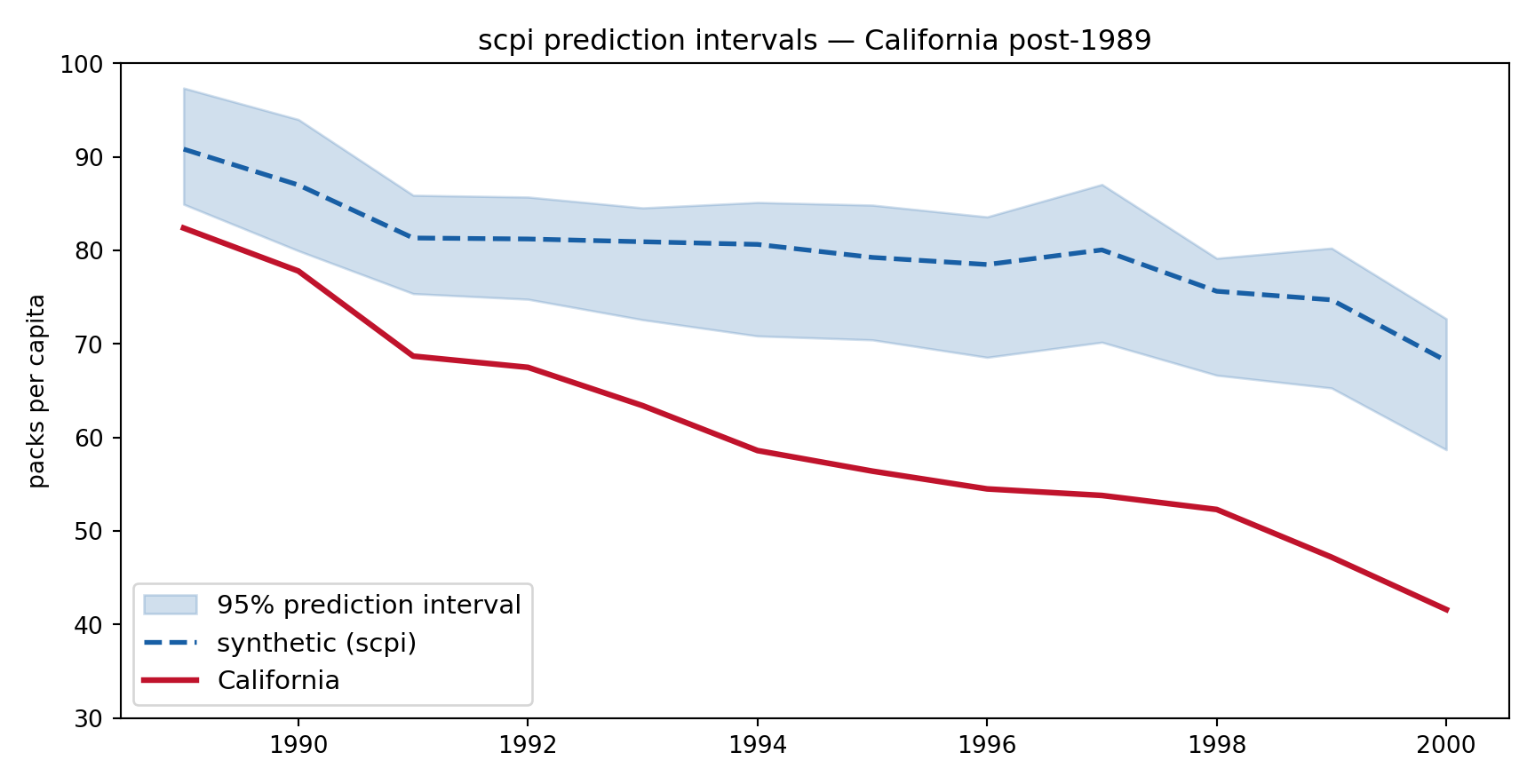
scpi prediction intervals — treat the counterfactual as a forecast and quantify its error.
The Inference Problem in Synthetic Control — Permutation Tests
Under the sharp null \(H_0: \tau_{it}=0\ \forall i,t\), the label “treated” could equally have fallen on any unit. So the placebo distribution of the test statistic (post/pre RMSPE ratio) across all units is its null distribution.
Firpo & Possebom (2018) turn the permutation test into a confidence set by test inversion. For a candidate constant effect \(\tau_0\), subtract it from the treated unit’s post-outcomes, re-run the permutation test on the adjusted data, and keep\(\tau_0\) if the test does not reject:
The set of non-rejected \(\tau_0\) is a \(1-\alpha\) confidence set for the (constant) effect.
They also generalize the placebo weights to a sensitivity parameter, allowing non-uniform assignment probabilities.
The permutation \(p\)-value assumes each unit was equally likely to be treated. Firpo–Possebom let you re-weight that assignment distribution and trace how the conclusion changes — a genuine sensitivity analysis for the design assumption.
Tooling
There is no CRAN/PyPI package named for Firpo–Possebom; the confidence set is obtained by inverting the placebo test that tidysynth/synth_runner already produce. Below we invert it directly — a thin wrapper over the package’s placebo machinery, not a re-implementation of the estimator.
# Test inversion. For a grid of constant effects tau0, subtract tau0 from# California's POST outcomes, recompute the post/pre MSPE ratio for California# and every (pre-fit-pruned) placebo donor, and take the permutation p-value.# The 95% confidence set is { tau0 : p(tau0) > 0.05 }. This is a thin wrapper# over tidysynth's placebo machinery, not a re-implementation of the estimator.ph <- sc %>%grab_synthetic_control(placebo =TRUE) %>%mutate(gap = real_y - synth_y)cap <- ph %>%group_by(.id) %>%summarise(pre =sqrt(mean(gap[time_unit <1989]^2)), .groups ="drop")keep <- cap$.id[cap$pre <=5* cap$pre[cap$.id =="California"]] # prune poor pre-fitspval <-function(tau0) { d <- ph %>%filter(.id %in% keep) %>%mutate(g =ifelse(.id =="California"& time_unit >=1989, gap - tau0, gap)) r <- d %>%group_by(.id) %>%summarise(ratio =sqrt(mean(g[time_unit >=1989]^2)) /sqrt(mean(g[time_unit <1989]^2)), .groups ="drop")mean(r$ratio >= r$ratio[r$.id =="California"])}grid <-seq(-40, 10, 1)pvals <-numeric(length(grid))for (i inseq_along(grid)) pvals[i] <-pval(grid[i])cset <-range(grid[pvals >0.05])
Permutation test (tidysynth): California MSPE ratio = 74.0, rank 3 of 39, p = 0.077
Inverting this test over a grid of constant effects tau0 gives the
Firpo–Possebom confidence set as { tau0 : p(tau0) > 0.05 } (code tab).
With one treated unit and the pre-outcome parity spec, the placebo \(p\)-value is marginal (\(\approx 0.08\)). This is typical: SC significance depends on the donor pool, the predictor set, and the pruning rule. The confidence set obtained by inverting the test conveys this uncertainty far better than a single star.
Re-running the inversion with non-uniform assignment weights (some units more plausibly “treatable” than others) widens or shifts the set — the Firpo–Possebom sensitivity report. A conclusion that survives a range of assignment distributions is robust.
* synth_runner reports the placebo distribution; invert it over a tau0 grid* in a loop (subtract tau0 from the treated post outcomes, re-rank) to build* the same confidence set. No single canned command exists.
library(scpi)donors <-setdiff(unique(ca$state), "California")sd <-scdata(df = ca, id.var ="state", time.var ="year", outcome.var ="cigsale",period.pre =1970:1988, period.post =1989:2000,unit.tr ="California", unit.co = donors,constant =FALSE, cointegrated.data =TRUE)res <-scpi(sd, e.method ="gaussian", sims =200, cores =1) # point + prediction intervalsscplot(res) # paths with PI band
---------------------------------------------------------------
Estimating Weights...
Quantifying Uncertainty
Treated unit 1: 20/200 iterations completed (10%)
Treated unit 1: 40/200 iterations completed (20%)
Treated unit 1: 60/200 iterations completed (30%)
Treated unit 1: 80/200 iterations completed (40%)
Treated unit 1: 100/200 iterations completed (50%)
Treated unit 1: 120/200 iterations completed (60%)
Treated unit 1: 140/200 iterations completed (70%)
Treated unit 1: 160/200 iterations completed (80%)
Treated unit 1: 180/200 iterations completed (90%)
Treated unit 1: 200/200 iterations completed (100%)
Year
Observed
Synthetic
PI lower
PI upper
1989
82.4
90.8
84.6
96.3
1992
67.5
81.2
75.1
85.7
1996
54.5
78.5
69.4
83.3
2000
41.6
68.2
58.7
72.6
The observed California outcome sits below the synthetic prediction interval in every post-year — the effect is statistically detectable period by period.
Code
import os, contextlibimport pandas as pd, numpy as np, matplotlib.pyplot as pltfrom scpi_pkg.scdata import scdatafrom scpi_pkg.scpi import scpica = pd.read_csv("../data/sc-california.csv")donors = [s for s in ca.state.unique() if s !="California"]sd = scdata(df=ca, id_var="state", time_var="year", outcome_var="cigsale", period_pre=np.arange(1970, 1989), period_post=np.arange(1989, 2001), unit_tr="California", unit_co=donors, constant=False, cointegrated_data=True)np.random.seed(14159)withopen(os.devnull, "w") as _f, contextlib.redirect_stdout(_f): # hide progress log res = scpi(sd, e_method="gaussian", sims=200, cores=1) # same estimator & intervals as Ryr = np.arange(1989, 2001)obs = np.asarray(res.Y_post).ravel(); synth = np.asarray(res.Y_post_fit).ravel()lo = np.asarray(res.CI_all_gaussian)[:, 0]; hi = np.asarray(res.CI_all_gaussian)[:, 1]fig, ax = plt.subplots(figsize=(9, 4.6))ax.fill_between(yr, lo, hi, color="#185FA5", alpha=0.2, label="95% prediction interval")ax.plot(yr, synth, color="#185FA5", lw=2, ls="--", label="synthetic (scpi)")ax.plot(yr, obs, color="#C0132C", lw=2.4, label="California")_ = ax.set(ylabel="packs per capita", ylim=(30, 100), title="scpi prediction intervals — California post-1989")ax.legend(fontsize=11); plt.tight_layout(); plt.show()
scpi across languages
scpi_pkg mirrors the R API almost one-to-one (scdata → scest/scpi), so the point estimate and prediction bands agree across languages.
No Stata port of scpi. Use synth_runner’s placebo inference for a design-based \(p\)-value, and R/Python scpi for prediction intervals.
Failing to reject parallel pre-trends is weak evidence — low power can hide violations. fect (Liu, Wang & Xu 2022) runs an equivalence test: it asks whether pre-treatment residuals are statistically indistinguishable from zero within a pre-set bound, a much stronger check than a non-significant \(F\).
Code
library(fect)# Placebo + equivalence diagnostics on a panel (here the known-truth sim panel).out <-fect(Y ~ D + X1 + X2, data = sim, index =c("unit", "time"),method ="ife", CV =TRUE, r =c(0, 5),se =TRUE, nboots =200, parallel =TRUE, cores =6,placeboTest =TRUE, placebo.period =c(-2, 0))plot(out, type ="equiv") # equivalence test on pre-treatment fit
What fect adds
fect unifies generalized SC, matrix completion and the equivalence/placebo tests under one interface — we use it heavily in Parts IV–VI. The equivalence and carryover tests are its distinctive contribution to validating a design, not just estimating it.
The fect equivalence/placebo suite is R-only. Python/Stata users validate pre-trends manually (event-study leads) or via pyfixest event studies; there is no packaged equivalent.
Many treated units, and treatment selected on latent factors: treated and control units load differently on common shocks, so difference-in-differences is biased — no amount of covariate control fixes it.
sc-simul.csv — a simulated interactive-fixed-effects panel with a known answer: \(N = 40\) units (10 treated), \(T = 30\), \(r = 2\) latent factors, treatment assigned on the loading of a trending factor. True average post-ATT = 3.75; DiD is provably biased.
Single-unit SC does not scale to many treated units.
TWFE / DiD assumes parallel trends, which factor confounding violates.
Adding \(X_1, X_2\) to the regression does not remove the latent-factor bias.
Generalized SC (IFE) — estimate the factor structure on controls, impute treated loadings from the pre-period, and reconstruct the counterfactual.
Cross-validated number of factors \(r\) and bootstrap confidence intervals.
ADH SC handles one treated unit. Many designs have many treated units (all sharing one adoption date). Stacking separate SCs is inefficient and gives no unified inference. Generalized synthetic control (Xu 2017) estimates a single interactive fixed effects (IFE) model on the whole panel.
\(\lambda_i' f_t\) — the same latent factor structure that justifies SC, now estimated explicitly.
Fit the factor model on controls, then impute each treated unit’s counterfactual \(\widehat{Y}_{it}^0\) from its estimated loadings.
SC’s convex weights are one way to match factor loadings; gsynth estimates the factors directly (a factor-analytic regression), so it needs no convexity.
Handles covariates, multiple treated units, and gives bootstrap inference.
Chooses the number of factors \(r\) by cross-validation — no manual tuning.
Estimate on controls. Using only never-treated units, fit the IFE model by iterated least squares to get \(\hat\beta\), the factors \(\hat f_t\) and control loadings.
Impute treated loadings. For each treated unit, regress its pre-treatment outcomes (net of covariates) on the estimated factors to recover its loading \(\hat\lambda_i\).
Predict the counterfactual. Form \(\widehat{Y}_{it}^0 = x_{it}'\hat\beta + \hat\lambda_i'\hat f_t\) for post-treatment \(t\); the ATT is the average of \(Y_{it}-\widehat{Y}_{it}^0\). Cross-validation picks \(r\); a parametric or nonparametric bootstrap gives standard errors.
subject to normalizations \(F'F/T = I_r\) and \(\Lambda'\Lambda\) diagonal. Then impute treated counterfactuals from \(\widehat{Y}_{it}^0 = x_{it}'\hat\beta + \hat\lambda_i'\hat f_t\).
A consistent ATT under a correct factor structure, even when treated and control units have different factor loadings (where DiD’s parallel-trends fails).
Cross-validated \(r\), bootstrap CIs, and a built-in dynamic ATT path.
\(N=40\) units (10 treated), \(T=30\), treatment from \(t=21\) (\(T_0=20\)), \(r=2\) factors.
Factor 1 trends strongly in time; the treated units are those with the largest loading on it.
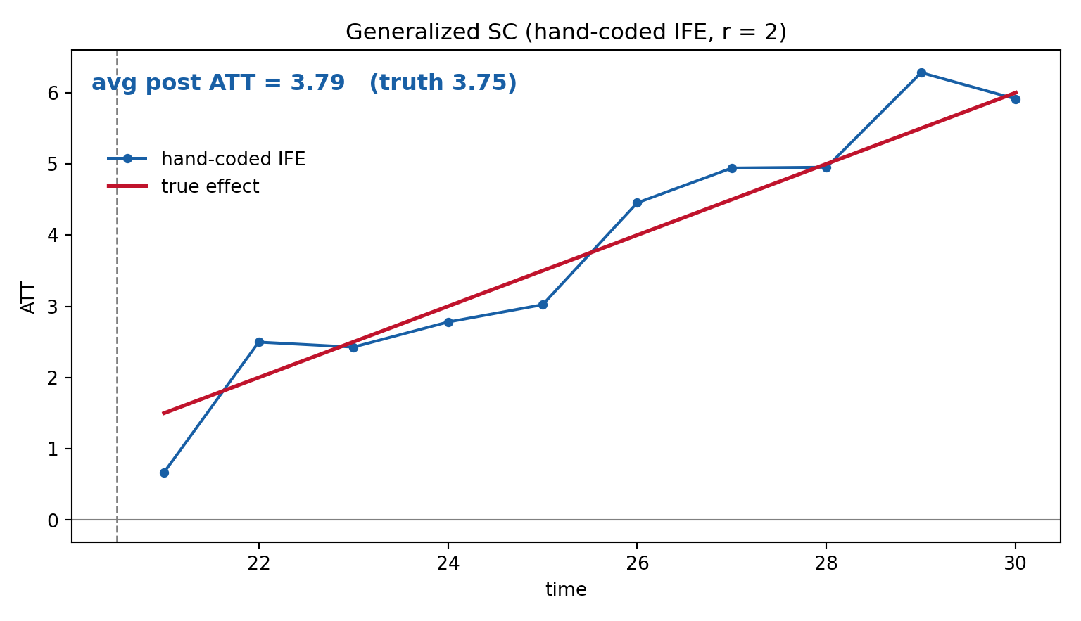
True dynamic ATT:\(\tau_t = 1 + 0.5\,(t - T_0)\), so the average post-treatment ATT is 3.75.
Because treated units load high on a trending factor, their counterfactual would have drifted up anyway. TWFE assumes parallel trends and attributes that drift to the treatment — so it overstates the effect. Generalized SC estimates the factor and removes the drift.
This is selection on an unobserved factor loading — exactly the confounding SC/IFE were built to defeat and DiD cannot.
The panel is written by synthetic-control-data.R (run once); R, Python and Stata all read ../data/sc-simul.csv.
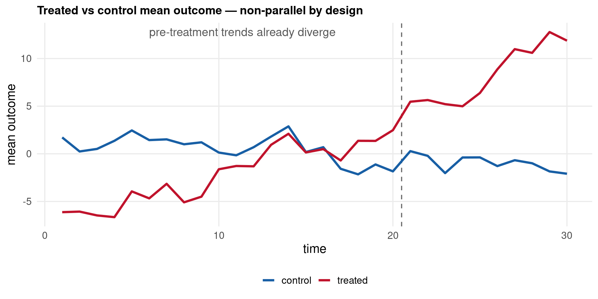
# Average outcome path, treated vs control. They DIVERGE pre-treatment already,# because treated units load high on the trending factor — the parallel-trends# assumption is violated by construction.agg <- sim %>%group_by(time, treated) %>%summarise(Y =mean(Y), .groups ="drop")ggplot(agg, aes(time, Y, color =factor(treated))) +geom_vline(xintercept =20.5, linetype ="dashed", color ="grey40") +geom_line(linewidth =1.3) +scale_color_manual(values =c("0"="#185FA5", "1"="#C0132C"),labels =c("control", "treated"), name =NULL) +labs(title ="Treated and control diverge BEFORE treatment (factor confounding)",x ="time", y ="mean outcome")
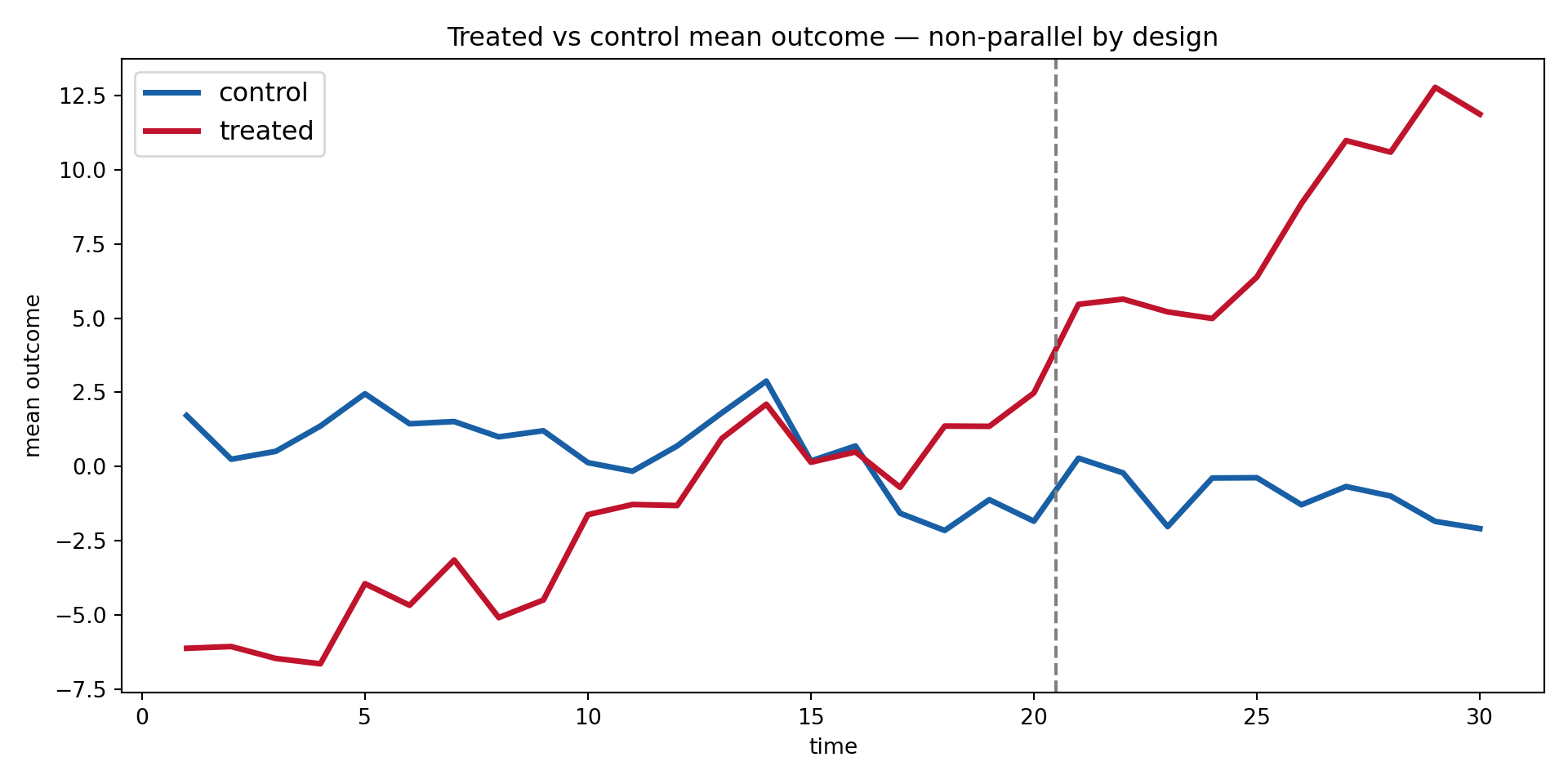
The two groups fan apart even before \(t=21\): a naive DiD reads that pre-existing divergence as a treatment effect.
Code
import pandas as pd, matplotlib.pyplot as pltsim = pd.read_csv("../data/sc-simul.csv")agg = sim.groupby(["time", "treated"]).Y.mean().reset_index()fig, ax = plt.subplots(figsize=(10, 5))for tv, col, lab in [(0, "#185FA5", "control"), (1, "#C0132C", "treated")]: g = agg[agg.treated == tv] ax.plot(g.time, g.Y, color=col, lw=2.6, label=lab)ax.axvline(20.5, ls="--", color="grey")_ = ax.set(xlabel="time", ylabel="mean outcome", title="Treated vs control mean outcome — non-parallel by design")ax.legend(fontsize=12); plt.tight_layout(); plt.show()
library(gsynth)g <-gsynth(Y ~ D + X1 + X2, data = sim, index =c("unit", "time"),force ="two-way", CV =TRUE, r =c(0, 5), # cross-validate r in 0..5se =TRUE, inference ="parametric", nboots =200,parallel =TRUE, cores =6, seed =14159)g$est.avg # average ATT, SE, CIg$r.cv # cross-validated number of factorsplot(g, type ="gap") # estimated dynamic ATT with CI
Cross-validated number of factors r = 1
gsynth ATT = 3.505 (SE 0.431, 95% CI [2.66, 4.35])
TRUE ATT = 3.750
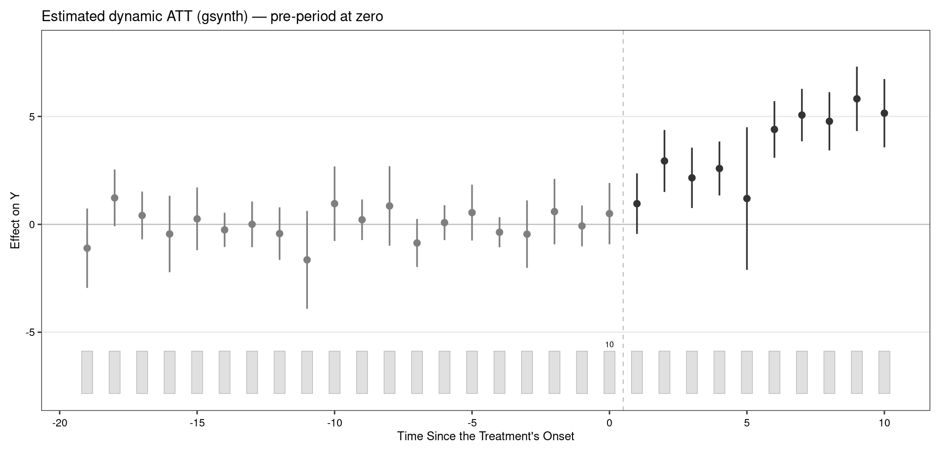
gsynth estimates an ATT of ≈ 3.51 with a 95% CI of about [2.66, 4.35] that comfortably covers the true 3.75, while cross-validation selects a parsimonious \(r=1\) factor.
There is no maintained gsynth port, but the Xu (2017) estimator is a short interactive-fixed-effects iteration — hand-coded here it recovers the known truth.
Code
import numpy as np, pandas as pd, matplotlib.pyplot as pltd = pd.read_csv("../data/sc-simul.csv")units = np.sort(d.unit.unique()); times = np.sort(d.time.unique()); T0 =20; r =2piv =lambda c: d.pivot(index="unit", columns="time", values=c).loc[units, times].valuesY, D = piv("Y"), piv("D").astype(bool); X1, X2 = piv("X1"), piv("X2")ever = d.groupby("unit").D.max().loc[units].values.astype(bool); co =~ever # controlsdef defactor(E, r, iters=100): # two-way FE + rank-r factors n, T = E.shape; a = np.zeros(n); b = np.zeros(T); L = np.zeros((n, T))for _ inrange(iters): a = (E - b[None,:] - L).mean(1); b = (E - a[:,None] - L).mean(0) U, s, Vt = np.linalg.svd(E - a[:,None] - b[None,:], full_matrices=False) L = (U[:, :r] * s[:r]) @ Vt[:r]return a, b, L, Vt[:r]beta = np.zeros(2) # alternate covariates <-> factorsfor _ inrange(50): E = Y - beta[0]*X1 - beta[1]*X2 aC, b, Lc, F = defactor(E[co], r) # FE + factors from controls only R = (Y[co] - aC[:,None] - b[None,:] - Lc).ravel() beta = np.linalg.lstsq(np.column_stack([X1[co].ravel(), X2[co].ravel()]), R, rcond=None)[0]Ft = F.T; pre = times <= T0; Yhat = np.zeros_like(Y)for i in np.where(ever)[0]: # treated loadings from pre-period yi = Y[i] - beta[0]*X1[i] - beta[1]*X2[i] - b c = np.linalg.lstsq(np.column_stack([np.ones(pre.sum()), Ft[pre]]), yi[pre], rcond=None)[0] Yhat[i] = beta[0]*X1[i] + beta[1]*X2[i] + b + c[0] + Ft @ c[1:]gap = Y - Yhatatt_t = np.array([gap[ever, ti][D[ever, ti]].mean() if D[ever, ti].any() else np.nanfor ti inrange(len(times))])att = gap[D & ever[:, None]].mean()true_t = np.where(times > T0, 1+0.5*(times - T0), 0.0)fig, ax = plt.subplots(figsize=(8, 4.6))ax.axhline(0, color="grey", lw=0.8); ax.axvline(T0 +0.5, ls="--", color="grey", lw=1)
<matplotlib.lines.Line2D object at 0x7b30a2331c90>
<matplotlib.lines.Line2D object at 0x7b30a23b5ea0>
No Stata command for generalized SC. xtdcce2/xthst touch interactive effects for other purposes, but there is no packaged Xu (2017) estimator. The R tab uses gsynth; the Python tab hand-codes the IFE iteration. In Stata the same algorithm would need a bespoke Mata loop, so this is a genuine R/Python-first method rather than a fragile port.
The contrast is stark: the true ATT is 3.75. Generalized SC lands on it; two-way FE is badly biased upward (≈ 12), because it mistakes the treated units’ factor-driven drift for a treatment effect.
The estimated post-treatment path tracks the true growing effect \(\tau_t = 1 + 0.5(t-T_0)\), and the pre-treatment gap sits at zero — the equivalence check passes.
When treatment is selected on latent factors, DiD is biased and no amount of covariate control fixes it (\(X_1, X_2\) are already in the TWFE regression). You must model the factor structure — that is what generalized SC and matrix completion do.
gsynth holds out pre-treatment periods and picks the \(r\) minimizing the cross-validated mean squared prediction error (MSPE). Too few factors → residual confounding; too many → overfitting noise.
Cross-validation selected r = 1 factor(s).
MSPE falls sharply from r=0 (no factors, = TWFE) to r=2, then rises (overfit).
At the chosen r=1 the ATT is 3.51 vs the truth 3.75.
With a weak factor, CV may pick \(r=0\) and collapse to TWFE — inspect the pre-treatment fit.
Report the ATT’s sensitivity to \(r\) (a robustness table) rather than a single CV pick.
fect offers the same CV plus equivalence tests on the pre-period fit.
# Generalized SC on the single-treated California panel: with one treated unit,# gsynth reduces to a factor-model synthetic control (r chosen by CV).ca$D <- ca$treatedgca <-gsynth(cigsale ~ D, data = ca, index =c("state", "year"),force ="two-way", CV =TRUE, r =c(0, 5),se =FALSE, parallel =FALSE, seed =14159)gca$att.avg
Generalized SC (California, r = 1): ATT = -13.89 packs
For comparison — ADH SC ≈ -19.5, Synthetic DiD ≈ -15.6 (Part VIII).
On real data, generalized SC gives an ATT in the same ballpark (≈ −14 packs) as ADH SC and synthetic DiD — reassuring agreement across very different estimators.
With one treated unit, gsynth is a factor-model SC; its estimate need not equal ADH’s exactly (different objective), but should be close.
The value of gsynth is realized with many treated units — the next Parts.
View the causal panel as a matrix with the treated cells missing. Recover them by exploiting the low-rank structure of the untreated outcomes — a matrix-completion problem.
Two known-truth panels: sc-stagger.csv — a staggered panel (many treated cells, diffuse factors, true ATT 4.13), MC’s sweet spot; and sc-simul.csv — a single strong factor, where MC deliberately struggles.
IFE fixes the number of factors \(r\); the truth may be diffuse or higher-rank.
With many treated cells scattered across time, per-unit loading imputation is fragile.
We want a method that regularizes the whole matrix, not a fixed-rank model.
MC-NNM — nuclear-norm (SVD soft-thresholding) completion of the outcome matrix.
Recovers the counterfactual on staggered / diffuse panels where factor models over- or under-fit.
Arrange outcomes in an \(N \times T\) matrix \(Y\). The treated (unit, period) cells are exactly the entries where we do not observe\(Y^0\) — they are missing. Causal inference becomes a matrix completion problem: fill in the missing \(Y^0\) entries from the observed ones.
The control entries are observed; the treated post-period entries are the holes to impute.
Assuming \(Y^0\) is (approximately) low rank — a few latent factors — lets us complete it.
A low-rank \(L^\star = U V'\)is a factor model: \(L_{it} = u_i' v_t\). So matrix completion and interactive fixed effects target the same object — but estimate it differently (regularization vs fixed-\(r\) factor extraction).
Matrix Completion — Nuclear-Norm Regularization, and How It Differs
Estimate \(L\) by least squares on the observed cells \(\mathcal{O}\), penalizing the nuclear norm\(\|L\|_\star\) (the sum of singular values) — the convex relaxation of matrix rank:
MC-NNM: a continuous penalty \(\zeta\) shrinks all singular values — no hard rank choice, more robust when the rank is unknown or the signal is diffuse across many small factors.
They optimize different things
Both target a low-rank \(Y^0\), but:
gsynth (IFE) does best when there are few, strong factors — it estimates them exactly.
MC-NNM does best when the signal is spread over many small factors, or the rank is unknown — the nuclear-norm penalty adapts smoothly.
On a panel dominated by one very strong factor (our sc-simul), the nuclear-norm penalty shrinks that big factor and leaves residual trend — MC-NNM is biased there while gsynth nails it.
On a panel with many treated cells and a diffuse low-rank structure (our staggered panel), MC-NNM recovers the truth as well as any factor model.
Lesson: match the tool to the factor structure; when unsure, report both and compare.
The MC-NNM paper argues nuclear-norm completion nests and generalizes SC and DiD, and is more robust across missing-data patterns (block, staggered, scattered) — at the cost of the transparent donor weights SC provides.
library(fect)# Staggered panel (many treated cells, diffuse factors): MC-NNM's sweet spot.mc <-fect(Y ~ D, data = stag, index =c("unit", "time"),method ="mc", CV =TRUE, se =FALSE, parallel =FALSE)mc$att.avg # recovers the true overall ATT (4.133)
Estimator
ATT
TRUE overall ATT
4.13
Matrix completion (MC-NNM)
4.04
Factor / IFE (fect)
4.05
Two-way FE / DiD
3.17
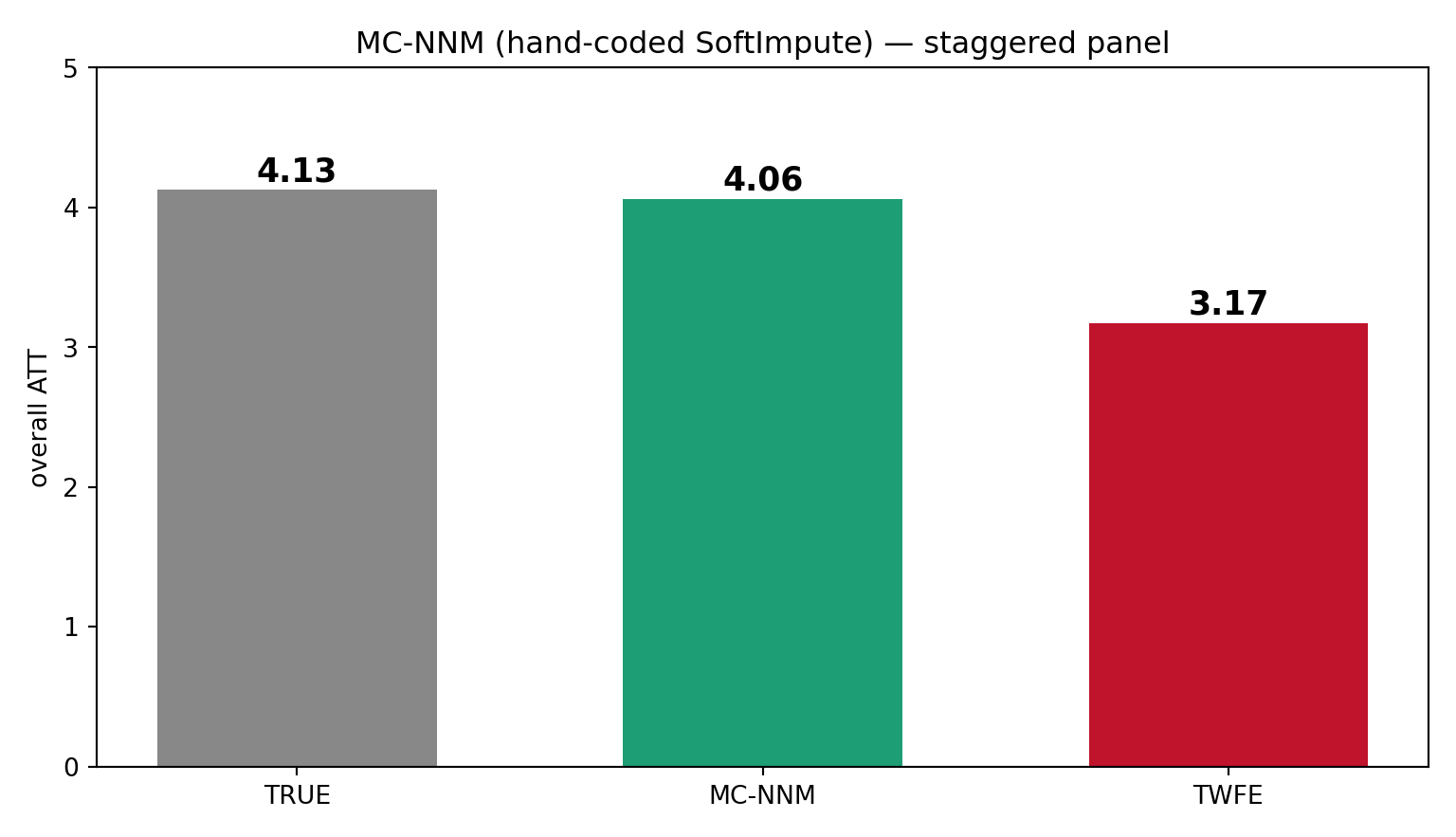
On the staggered panel (many treated cells), MC-NNM recovers the true ATT of 4.13 — matching the factor model and correcting TWFE’s downward bias.
Estimator
ATT
TRUE ATT
3.75
Generalized SC (IFE)
3.51
Matrix completion (MC-NNM)
7.29
On the single-strong-factor panel, MC-NNM over-shrinks the dominant factor and is biased — a faithful illustration of the trade-off above.
The causaltensor package pins numpy<2 and is fragile here — but MC-NNM is just SoftImpute: fill the treated cells with the current fit, soft-threshold the SVD, repeat. A few lines of NumPy recover the truth.
Code
import numpy as np, pandas as pd, matplotlib.pyplot as pltd = pd.read_csv("../data/sc-stagger.csv")units = np.sort(d.unit.unique()); times = np.sort(d.time.unique())Y = d.pivot(index="unit", columns="time", values="Y").loc[units, times].valuesD = d.pivot(index="unit", columns="time", values="D").loc[units, times].astype(bool).valuesO =~D # observed = untreated cellsdef mc_nnm(Y, O, lam, iters=400, tol=1e-6): # SoftImpute + two-way FE n, T = Y.shape; M = np.zeros_like(Y); a = np.zeros(n); b = np.zeros(T)for _ inrange(iters): M_old = M.copy() Z = np.where(O, Y, M + a[:, None] + b[None, :]) # fill treated cells with fit a = (Z - b[None, :] - M).mean(1); b = (Z - a[:, None] - M).mean(0) U, s, Vt = np.linalg.svd(Z - a[:, None] - b[None, :], full_matrices=False) s = np.maximum(s - lam, 0.0); M = (U * s) @ Vt # nuclear-norm soft-thresholdif np.linalg.norm(M - M_old) < tol * np.linalg.norm(M_old): breakreturn M + a[:, None] + b[None, :]fit = mc_nnm(Y, O, lam=3.0)att_mc = (Y[D] - fit[D]).mean()dum =lambda s: pd.get_dummies(s, drop_first=True).astype(float).values # TWFE contrastXall = np.column_stack([np.ones(len(d)), d.D.values.astype(float), dum(d.unit), dum(d.time)])att_tw = np.linalg.lstsq(Xall, d.Y.values, rcond=None)[0][1]labs = ["TRUE", "MC-NNM", "TWFE"]; vals = [4.13, att_mc, att_tw]fig, ax = plt.subplots(figsize=(8, 4.6))ax.bar(labs, vals, color=["#888888", "#1D9E75", "#C0132C"], width=0.6)for x, v inenumerate(vals): ax.text(x, v +0.06, f"{v:.2f}", ha="center", fontsize=13, fontweight="bold")_ = ax.set(ylabel="overall ATT", ylim=(0, 5), title="MC-NNM (hand-coded SoftImpute) — staggered panel")plt.tight_layout(); plt.show()
No packaged command, but MC-NNM is just SoftImpute — a short Mata SVD-thresholding loop recovers the truth and beats TWFE, matching the Python tab.
Code
quietly import delimited "../data/sc-stagger.csv", clearquietlykeep unit time ydquietly reghdfe yd, absorb(unit time) // two-way FE / DiD, for contrastlocal att_tw = _b[d]quietlyreshapewideyd, i(unit) j(time) // units x time, widequietlydsy*local yv `r(varlist)'quietlydsd*local dv `r(varlist)'mata:Y = st_data(., tokens(st_local("yv"))) // outcome matrixD = st_data(., tokens(st_local("dv"))) // treatment maskO = (D :== 0) // observed = untreated cellsn = rows(Y); T = cols(Y); lam = 3M = J(n, T, 0); a = J(n, 1, 0); b = J(1, T, 0)for (it = 1; it <= 400; it++) { Mold = M Z = O:*Y + (1:-O):*(M :+ a :+ b) // fill treated cells with the fit a = rowsum(Z :- b :- M) :/ T // two-way fixed effects b = colsum(Z :- a :- M) :/ n u=.; s=.; v=.svd(Z :- a :- b, u, s, v) // SVD of the FE-removed matrixs = s :- lam; s = s :* (s :> 0) // nuclear-norm soft-threshold M = (u :* s') * vif (sqrt(sum((M:-Mold):^2)) < 1e-6*sqrt(sum(Mold:^2))) break}gap = Y :- (M :+ a :+ b)st_local("att_mc", strofreal(sum(D :* gap)/sum(D), "%9.3f"))enddiastext"TRUE overall ATT = 4.133"diastext"MC-NNM (SoftImpute) = `att_mc'"diastext"Two-way FE / DiD = " %5.3f `att_tw'
------------------------------------------------- mata (type end to exit) ----------------------------------------------
: Y = st_data(., tokens(st_local("yv")))            // outcome matrix

: D = st_data(., tokens(st_local("dv")))            // treatment mask

: O = (D :== 0)                                      // observed = untreated cells

: n = rows(Y); T = cols(Y); lam = 3

: M = J(n, T, 0); a = J(n, 1, 0); b = J(1, T, 0)

: for (it = 1; it <= 400; it++) {
>     Mold = M
>     Z = O:*Y + (1:-O):*(M :+ a :+ b)              // fill treated cells with the fit
>     a = rowsum(Z :- b :- M) :/ T                  // two-way fixed effects
>     b = colsum(Z :- a :- M) :/ n
>     u=.; s=.; v=.
>     svd(Z :- a :- b, u, s, v)                     // SVD of the FE-removed matrix
>     s = s :- lam; s = s :* (s :> 0)               // nuclear-norm soft-threshold
>     M = (u :* s') * v
>     if (sqrt(sum((M:-Mold):^2)) < 1e-6*sqrt(sum(Mold:^2))) break
> }

: gap = Y :- (M :+ a :+ b)

: st_local("att_mc", strofreal(sum(D :* gap)/sum(D), "%9.3f"))

: end
------------------------------------------------------------------------------------------------------------------------

TRUE overall ATT    = 4.133

MC-NNM (SoftImpute) = 4.063

Two-way FE / DiD    = 3.175
As the nuclear-norm penalty \(\zeta\) shrinks, the completed matrix moves from rank-0 (just fixed effects, = TWFE) to a high-rank interpolation of the pre-period. Cross-validation picks the \(\zeta\) minimizing held-out MSPE.
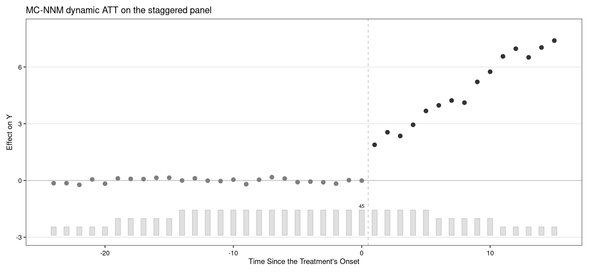
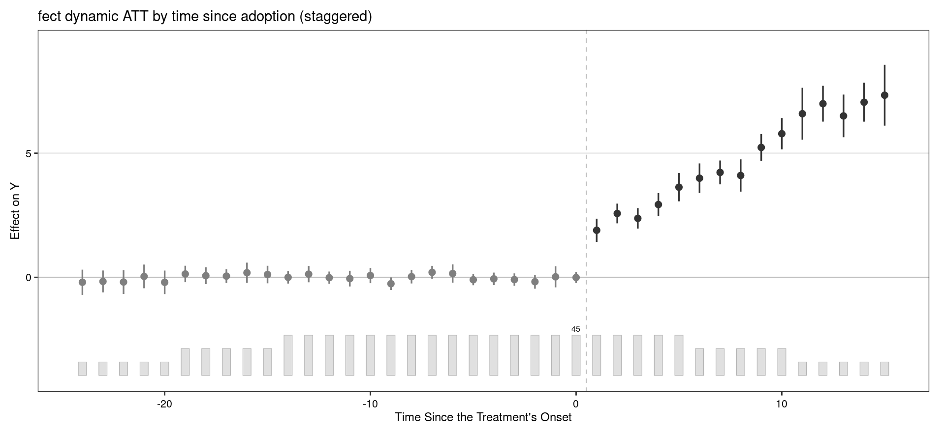
The estimated dynamic effect grows with time-since-adoption, tracking the true \(\tau_k = 2 + 0.4k\), and the pre-period gap sits at zero.
Small \(\zeta\) → rich completion, risk of overfitting the pre-period.
Large \(\zeta\) → close to TWFE, risk of under-fitting the factor structure.
CV balances the two; always inspect the pre-treatment fit before trusting the post-period gap.
Units adopt treatment at different times (cohorts), with heterogeneous, dynamic effects. Pooled SC and static two-way FE are biased under staggering.
sc-stagger.csv — a staggered known-truth panel: multiple cohorts adopting over time, cohort effects \(\tau_k = 2 + 0.4k\) that grow with exposure, overall ATT ≈ 4.13.
TWFE uses already-treated units as controls → negative weights and forbidden comparisons.
Pooled SC ignores cohort heterogeneity and dynamic effects.
A single ATT hides the dynamic path you actually care about.
Partial-pooling SC (multisynth) — a separate fit per cohort, shrunk toward the pool.
fect for staggered designs — dynamic effects plus placebo / carryover tests.
Staggered synthetic DiD (sdid) — unit + time weights per cohort.
The Staggered Adoption Problem — and Why Pooled SC & TWFE Fail
Real policies roll out at different times across units (states adopt a law in different years). Each treated unit has its own adoption date\(g_i\) and its own donor pool of not-yet-treated units.
The estimand is now a collection of cohort effects, plus their weighted average.
Effects usually depend on time since adoption\(k = t - g_i\) (a dynamic path).
Static two-way FE is biased under staggering, even with parallel trends. Goodman-Bacon (2021) shows the TWFE coefficient is a weighted average of all 2×2 DiDs — including “forbidden” comparisons that use already-treated units as controls. With dynamic effects, those comparisons subtract post-treatment outcomes and bias the estimate (often toward zero or even the wrong sign).
sc-stagger.csv: \(N=60\) units, \(T=30\). Three cohorts adopt at \(g \in \{16, 21, 26\}\) (15 units each); 15 are never treated. Cohorts are assigned at random (timing is unconfounded), factors are mild, and the dynamic effect grows:
\[\tau_k = 2 + 0.4\,k, \qquad k = t - g_i \ge 0.\]
True overall ATT (average over all treated cells) = 4.133.
The only source of TWFE bias here is staggering × dynamic effects (Goodman-Bacon), not factor confounding — a clean isolation of the staggered problem.
N = 60 units, T = 30; cohorts g in {16, 21, 26} + never-treated.
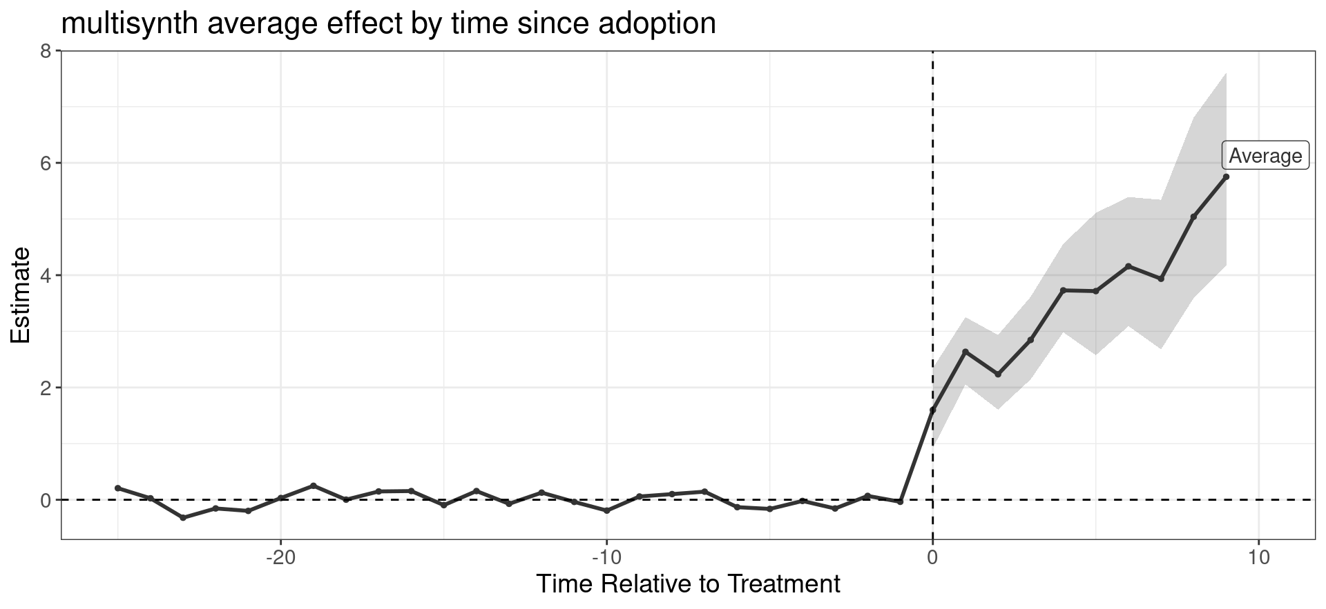
library(augsynth)stag$trt <- stag$D# Partial-pooling SC: one synthetic control per treated unit, shrunk toward a# pooled fit. nu = 0 → separate SCs; nu = 1 → fully pooled; default picks it by CV.ms <-multisynth(Y ~ trt, unit, time, data = stag, n_leads =10)summary(ms)$att # cohort-time and averaged effects with SEs
multisynth average ATT (over the balanced lead window) = 3.27 (SE 0.33)
True overall ATT = 4.133
multisynth gives a partial-pooling average ATT in the right neighbourhood, with per-cohort effects available for inspection.
multisynth is R-only (augsynth). Stata users use sdid (next); Python has no partial-pooling SC — pysyncon handles only single-treated designs.
fect for Staggered Designs — Dynamic Effects & Carryover
Placebo / equivalence test — hides the last few pre-periods and checks the model predicts them within an equivalence bound (a strong pre-trend test).
Carryover test — hides the first few post-treatment periods of already-treated units to check the effect does not leak into the (assumed clean) control periods.
A staggered design assumes no anticipation (clean pre-periods) and no carryover (a treated unit does not contaminate later control comparisons). fect’s tests make both falsifiable, turning assumptions into diagnostics. Passing them is what makes the recovered 4.13 credible.
R’s synthdid estimates a single adoption date via synthdid_estimate(). For staggered adoption you loop over cohorts — one estimate per adoption year, each using the not-yet-treated units as donors — then aggregate the cohort effects weighted by cohort size. This is exactly the recipe Stata’s sdid automates. The packaged R routes for staggered designs are fect and augsynth::multisynth, shown on the previous slides.
No maintained Python package implements staggered Synthetic DiD: mlsynth.SDID (used on the block-treatment slide, Part VIII) assumes a single adoption date. As in R, you would loop cohort-by-cohort and aggregate. For staggered work in Python the practical routes are event-study estimators (pyfixest, differences); the reference staggered-SDID implementation remains Stata sdid.
Code
quietly import delimited "../data/sc-stagger.csv", clearquietlydestring_all, replace* sdid handles staggered adoption natively: it runs SDID cohort-by-cohort and* aggregates. The treatment variabled is 1 for treated unit-periods.sdid y unit time d, vce(noinference) method(sdid)
Synthetic Difference-in-Differences Estimator

-----------------------------------------------------------------------------
           y |     ATT     Std. Err.     t      P>|t|    [95% Conf. Interval]
-------------+---------------------------------------------------------------
           d |   3.81222          .        .        .           .           .
-----------------------------------------------------------------------------
95% CIs and p-values are based on large-sample approximations.
Refer to Arkhangelsky et al., (2021) for theoretical derivations.
All three staggered estimators — multisynth, fect, and staggered sdid — target the same cohort/overall ATT and agree up to their differing weighting schemes, correcting the static-TWFE bias.
Period by period, fect’s dynamic estimates track the true\(\tau_k = 2 + 0.4k\).
For staggered designs, always report the dynamic (event-study) path, not just one number. A single ATT hides heterogeneity across cohorts and time-since-adoption — and hides the very dynamics that break static TWFE.
When the treated unit sits near or outside the donor convex hull, plain SC cannot fit the pre-period and is biased toward the interior. Can we correct that bias without extrapolating wildly?
Same California Prop 99 panel — here the pre-fit is already good, so the augmentation is a small correction; the value is seeing how much it moves the estimate.
Plain SC refuses to extrapolate → biased for outliers, with a visibly poor fit.
Regression / IFE extrapolate freely → can “fit” anything, dangerously.
We want a principled middle.
Augmented SC — SC first, then a ridge-penalized outcome-model correction of the residual imbalance.
Small, penalized extrapolation that stays close to convex.
Negative weights that quantify the extrapolation instead of hiding it.
The Bias of Synthetic Control — and the Augmented Ridge Fix
SC is credible only with a near-perfect pre-fit. When no convex combination matches the treated unit (imperfect fit), SC carries a bias proportional to the residual imbalance. Ben-Michael, Feller & Rothstein (2021) make this bias explicit and correct it.
Fit an outcome model (e.g. ridge regression) to predict the residual imbalance, and subtract its estimate — an augmentation exactly analogous to bias-corrected matching or augmented IPW (the “doubly robust” idea).
Augmented SC
Let \(\hat w^{\text{SC}}\) be the SC weights and \(\hat m(\cdot)\) an outcome model fit on the donors. The augmented estimator corrects the SC counterfactual for its remaining pre-treatment imbalance:
The bracket is the model’s prediction of the imbalance SC could not close. With a ridge outcome model this is Ridge-ASCM. If SC already balances perfectly, the correction is zero and you recover plain SC.
The price: the correction can make weights negative — a small, penalized amount of extrapolation. The ridge penalty keeps it minimal.
Plain SC: no extrapolation, but biased if the pre-fit is imperfect.
Augmented SC: removes that bias by allowing a small, penalized extrapolation (possibly negative weights).
The ridge penalty \(\lambda\) controls how much extrapolation is permitted — \(\lambda \to \infty\) recovers plain SC.
Augmented SC nests SC (no augmentation), regression (full augmentation), and everything between — a continuum from “trust the convex hull” to “trust the outcome model.”
Negative Weights & Extrapolation
Negative weights are not a bug here — they are the point
They let the synthetic unit extrapolate just enough to close a pre-treatment gap SC alone could not. The ridge penalty keeps the extrapolation small and disciplined. Report the magnitude of the correction: a large one warns that SC was failing and the result leans on the outcome model.
Inspect how far the augmented weights depart from the simplex.
Report both plain SC and augmented SC — agreement is reassuring; divergence flags an extrapolation-sensitive result.
Augmented SC is most valuable exactly when plain SC’s pre-fit is poor.
import pandas as pd, matplotlib.pyplot as pltfrom pysyncon import Dataprep, AugSynthca = pd.read_csv("../data/sc-california.csv"); pre =list(range(1970, 1989))dp = Dataprep(foo=ca, dependent="cigsale", unit_variable="state", time_variable="year", treatment_identifier="California", controls_identifier=[s for s in ca.state.unique() if s !="California"], predictors=[], predictors_op="mean", time_predictors_prior=pre, special_predictors=[("cigsale", [y], "mean") for y in pre], time_optimize_ssr=pre)aug = AugSynth(); aug.fit(dp) # ridge-augmented SC (pysyncon)Y = ca.pivot(index="year", columns="state", values="cigsale")w = pd.Series(aug.W, index=dp.controls_identifier)gap = Y["California"] - (Y[w.index] * w.values).sum(axis=1)att = gap[Y.index >=1989].mean()# print(...) is silently dropped for this chunk (it follows a figure chunk, a# known reticulate/knitr issue on this machine), so the two result lines are# drawn as plain monospace text — mirroring the R cat() and Stata display output.lines = [f"Augmented SC (Ridge-ASCM): ATT = {att:6.2f} packs per capita",f"Min donor weight = {w.min():6.3f} (negative = extrapolation)"]fig, ax = plt.subplots(figsize=(8, 1.4)); ax.axis("off")for i, ln inenumerate(lines): ax.text(0.0, 0.75-0.5* i, ln, transform=ax.transAxes, family="monospace", fontsize=15, va="top")plt.tight_layout(); plt.show()
Code
quietly import delimited "../data/sc-california.csv", clearquietlydestring_all, replaceencode state, gen(id)xtset id yearquietlysummarize id if state=="California", meanonlylocalca = r(mean)* every pre-treatment yearof cigsale is a predictor (the parity spec)local predsforvaluesy = 1970/1988 {local preds `preds' cigsale(`y')}* allsynth (Wiltshire) = SC + regression bias correction. Like synth it floods* a long optimizer log that breaks Statamarkdown's capture, so the fit runs* here (silent) and the numbers are reported in the next chunk.allsynth cigsale `preds', trunit(`ca') trperiod(1989) bcorrect(merge) keep(_asc, replace) nograph
Code
quietlyuse _asc, clearquietlysummarize gap_bc if _time >= 1989 & _time < .displayastext"Augmented SC (bias-corrected ATT): "as result %6.2f r(mean) astext" packs per capita"quietlysummarize gap if _time >= 1989 & _time < .displayastext"Plain SC gap (for contrast) : "as result %6.2f r(mean) astext" packs per capita"
Augmented SC (bias-corrected ATT): -12.38 packs per capita


Plain SC gap (for contrast)      : -19.48 packs per capita
ASC vs ADH — Results Comparison
Method
ATT (packs)
Extrapolation
ADH synthetic control
-19.5
none (convex)
Augmented SC (ridge)
-16.0
small, penalized
Synthetic DiD
-15.6
unit + time weights
Generalized SC (IFE)
-13.9
factor model
All four estimators agree on a large negative effect
(≈ −15 to −20 fewer packs per capita) despite very different assumptions. That convergence across methods — convex weights, penalized extrapolation, unit+time weights, factor models — is the strongest evidence that Prop 99 genuinely cut smoking.
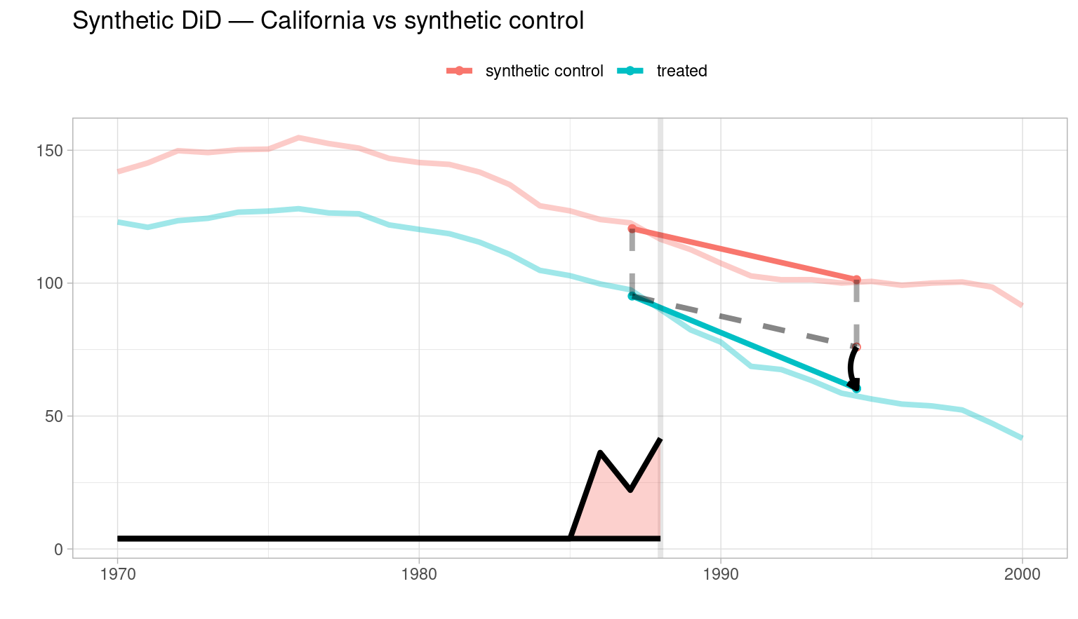
The unit weights\(\hat\omega_i\) are chosen (with a ridge penalty) so the weighted control pre-trend is parallel to the treated unit; the time weights\(\hat\lambda_t\) so each control’s weighted pre-period average predicts its post-period level.
Set \(\hat\lambda_t\) equal and \(\hat\omega_i\) to the simplex SC weights → you recover SC. Set both to equal weights → you recover DiD. SDID is the interior point that borrows strength from both.
The three estimators are nested — same data, same objective, different weight restrictions. On California this makes them directly comparable, and the gap between them is informative about which assumptions bite.
library(synthdid)# panel.matrices reshapes the long CSV into the Y matrix + (N0, T0) split.pm <-panel.matrices(ca, unit ="state", time ="year",outcome ="cigsale", treatment ="treated")tau_sdid <-synthdid_estimate(pm$Y, pm$N0, pm$T0) # unit + time weightstau_sc <-sc_estimate(pm$Y, pm$N0, pm$T0) # SC: time weights equaltau_did <-did_estimate(pm$Y, pm$N0, pm$T0) # DiD: both weights equalc(SDID = tau_sdid, SC = tau_sc, DID = tau_did)
Synthetic DiD : ATT = -15.60 (placebo SE 8.38)
Synthetic ctrl: ATT = -19.62
Diff-in-Diff : ATT = -27.35
Code
from mlsynth import SDID # mlsynth ports Arkhangelsky et al. to Pythonca = pd.read_csv("../data/sc-california.csv")res = SDID(dict(df=ca, outcome="cigsale", treat="treated", unitid="state", time="year", display_graphs=False)).fit()print(res.att) # -15.6, matches R synthdid to the digit
Code
* sdid (Clarke, Pailañir, Arkhangelsky, Imbens) — the official Stata portimport delimited "../data/sc-california.csv", clearquietlydestring_all, replacesdid cigsale state year treated, vce(placebo) reps(200) seed(14159)* ATT = -15.60, identical to R synthdid (exact numerical parity)
(encoding automatically selected: ISO-8859-1)
(4 vars, 1,209 obs)


Placebo replications (200). This may take some time.
----+--- 1 ---+--- 2 ---+--- 3 ---+--- 4 ---+--- 5
..................................................     50
..................................................     100
..................................................     150
..................................................     200


Synthetic Difference-in-Differences Estimator

-----------------------------------------------------------------------------
     cigsale |     ATT     Std. Err.     t      P>|t|    [95% Conf. Interval]
-------------+---------------------------------------------------------------
     treated | -15.60383    9.22192    -1.69    0.091   -33.67846     2.47080
-----------------------------------------------------------------------------
95% CIs and p-values are based on large-sample approximations.
Refer to Arkhangelsky et al., (2021) for theoretical derivations.
Exact cross-language parity
R synthdid = Python mlsynth = Stata sdid all return ATT ≈ −15.6. The three estimates on the same panel — DiD −27.3, SC −19.6, SDID −15.6 — show how much the equal-weight DiD over-states the effect by leaning on parallel trends that do not hold.
With a single treated unit, SDID’s standard analytic variance is unavailable. Arkhangelsky et al. propose a placebo variance: reassign the treatment to each control in turn, refit, and use the spread of the placebo estimates. This is the vce(placebo) / method = "placebo" route.
With several treated units, a fast jackknife (leave-one-unit-out) variance is available and consistent. It is the default when the design supports it; for one treated unit it degenerates, so placebo is used instead.
The placebo SE for California is large (≈ 9), so the 95% interval includes effects far from the point estimate. As with the Part III permutation inference, one treated unit buys a sharp point estimate but weak significance — the number to report alongside −15.6.
Unit & Time Weights — What SDID Chose
Code
# synthdid's own plot overlays treated vs synthetic paths and draws the# time weights as a ribbon along the x-axis — the whole estimator in one figure.plot(tau_sdid, line.width =1.4, point.size =1.6) + ggplot2::labs(title ="Synthetic DiD — California vs synthetic control") + ggplot2::scale_x_continuous(breaks =seq(1970, 2000, by =5)) ggthemes::theme_clean(base_size =18)
Reading the SDID figure
The figure shows the treated and synthetic paths, the arrow whose length is the estimated effect, and the shaded time weights — the periods SDID leaned on. A handful of controls (Nevada, Montana, Utah, Colorado) carry most of the unit weight, echoing the ADH SC donor set from Part I.
\(\mu_t\) is a local-level (or local-linear) trend; \(\boldsymbol\beta\) carries a spike-and-slab prior so most donors are shrunk to exactly zero — automatic donor selection.
The counterfactual is the posterior predictive \(p(\tilde y_t \mid \text{pre-period data})\) pushed into the post-period. The effect is \(\phi_t = y_t^{\text{obs}} - \tilde y_t\), and its whole posterior — pointwise and cumulative — is reported with credible intervals.
Unlike ADH SC, the weights \(\boldsymbol\beta\) are not restricted to the simplex — this is a regression counterfactual with a selection prior, closer in spirit to the augmented and penalized variants than to convex SC.
from causalimpact import CausalImpact # statsmodels-based reimplementationca = pd.read_csv("../data/sc-california.csv")wide = ca.pivot(index="year", columns="state", values="cigsale")# focus on the ADH donor states + a datetime index (the default fit is fragile# with all 38 collinear donors — it can diverge).don = ["Utah", "Nevada", "Montana", "Colorado", "Connecticut"]data = wide[["California"] + don].copy()data.index = pd.period_range("1970", periods=len(data), freq="Y").to_timestamp()ci = CausalImpact(data, [data.index[0], pd.Timestamp("1988")], [pd.Timestamp("1989"), data.index[-1]])print(ci.summary()) # avg effect ~ -10, tighter interval than R's BSTS
* No dedicated Bayesian structural-TS synthetic-control package ships for Stata.* Stata has a general Bayesian engine (bayes: / bayesmh) and bsts is not ported,* so Bayesian SC in the BSTS sense is an R/Python method.* For a Bayesian *panel* alternative in Stata, see the manual "bayes: regress".display"Bayesian SC (BSTS): use R CausalImpact or Python causalimpact."
No exact cross-engine parity — and that is the lesson
R CausalImpact uses Google’s spike-and-slab BSTS (wide priors → avg −22, wide CI); Python causalimpact uses a statsmodels structural model (avg −10, tighter CI). Same data, same model class, different priors and variance estimation → different posteriors. Bayesian answers are conditional on the prior; report which engine and prior you used.
Posterior Effect — Pointwise & Cumulative
Code
# CausalImpact's plot stacks three panels: observed vs counterfactual,# the pointwise effect, and the cumulative effect — each with a 95% band.plot(impact)
Reading the three panels
Top: California (solid) vs the BSTS counterfactual (dashed) with its credible band. Middle: the pointwise effect widens as the forecast extends. Bottom: the cumulative effect — the total packs-per-capita averted — with an interval that grows through the post-period. The band excludes zero for the middle post-years, matching the tail-area \(p\).
A hidden confounder drives both the treated unit and the donors, so plain SC and parallel-trends are invalid — but we have negative-control proxies that can rescue identification.
sc-proximal.csv — a simulated panel with a latent confounder: one treated unit and 20 donors, each carrying two series (an outcome \(W\) and a proxy \(Z\)), with a known ATT of −15.
Donors are contaminated by the same confounder → SC weights are biased.
Parallel trends is violated by the shared latent driver.
Standard tools cannot tell the confounder from the effect.
Proximal inference — an outcome bridge function identified through negative-control proxies.
Solves a Fredholm moment equation by GMM / 2SLS, with a sandwich variance.
Recovers the ATT under latent confounding where naive DiD cannot.
When the Donors Hide a Confounder — Proximal Identification
Every method so far assumes the donors, once weighted, reconstruct the treated unit’s untreated potential outcome. If a latent factor drives both the treated unit and the donors in a way convex weights cannot untangle, SC is biased — and no diagnostic on the donors alone reveals it.
Shi, Miao, Hu & Tchetgen Tchetgen (2023) import proximal causal inference: split the auxiliary series into two roles that stand in for the unseen confounder \(U\).
Negative-control outcomes\(W\) — donors not affected by the treatment.
Negative-control exposures / proxies\(Z\) — a second set of series correlated with \(U\) but conditionally independent of \(W\).
A bridge function links \(W\) and \(Z\); solving it identifies the ATT even under the hidden confounder.
It weakens the core SC assumption — no longer “the donors span the counterfactual,” but “there exist valid negative controls.” That is a genuinely different, testable-in-parts identification, and tooling is new (Python mlsynth).
Let \(U_t\) be the hidden confounder, \(W_t\) the negative-control outcomes and \(Z_t\) the negative-control proxies. Assume an outcome bridge\(h\) with
a Fredholm integral equation solved by GMM/2SLS. The post-period counterfactual is \(\hat h(W_t)\); the ATT is \(Y_t - \hat h(W_t)\) averaged over post-periods, with a GMM sandwich variance.
Proximal SC needs a genuine proxy variable on the donor units — California Prop 99 carries only one series per state, so it cannot identify a proximal model. We use sc-proximal.csv: one treated unit and 20 donors, each donor carrying two measured series (an outcome \(W\) and a proxy \(Z\)), both driven by a latent confounder, with a known ATT of −15. This lets us check the estimator against ground truth.
# No proximal-synthetic-control package ships for R yet. The proximal# framework is available via Python `mlsynth`; a general negative-control /# proximal-causal toolkit in R (e.g. GMM by hand with `gmm`) would have to be# hand-built, which this deck avoids in favour of the maintained package.message("Proximal SC: use Python `mlsynth` (PROXIMAL). No R package as of 2026.")
* No proximal synthetic-control package exists for Stata.display"Proximal SC: Python mlsynth only."
Proximal recovers the truth; naive DiD does not
PI returns ATT ≈ −15.6 (95% CI ≈ [−19.6, −11.6]), covering the known −15, while the confounder-blind DiD is pulled to ≈ −10 — biased toward zero by exactly the hidden factor the negative controls neutralise.
Pre-treatment, the proximal counterfactual tracks the treated unit (the bridge function is fit there). Post-treatment it separates — the observed series drops below the counterfactual by the estimated effect. Because the counterfactual is built from negative controls rather than a convex donor fit, it stays valid under the latent factor that would bias plain SC.
Python — mlsynth.PROXIMAL(..., methods = ["PI"]); the outcome bridge solved by GMM with a sandwich variance.
Requires genuine negative controls — a proxy \(Z\) independent of \(W\) given the confounder \(U\).
Recovers the truth (≈ −15) where naive DiD does not (≈ −10).
The counterfactual is built from proxies, not a convex donor fit.
Donor proxies vs surrogates — which series play \(W\) and \(Z\).
Method — PI (proximal inference) vs other mlsynth options.
Pre-period length — identifies the bridge function.
Part XI — Comparison & Practical Guidance
βουλεύματʼ ἔπη τʼ ἔστιν ἀκοῦσαι.
here are counsels, and words worth hearing
Αἰσχύλος, Προμηθεὺς δεσμώτης 1055
The Whole Family on One Panel
Method
California ATT
Weights
Key assumption
ADH synthetic control
-19.5
convex (simplex)
treated in convex hull
Penalized SC
-19
convex + penalty
sparse donor set
Augmented SC (ridge)
-16
convex + ridge correction
small extrapolation OK
Generalized SC (IFE)
-13.9
factor loadings
few common factors
Matrix completion (MC-NNM)
n/a (1 unit)
low-rank fill-in
low-rank + MAR
Synthetic DiD
-15.6
unit + time
parallel after reweighting
Bayesian SC (BSTS)
-22
spike-and-slab regression
correct state-space + prior
Every method that California can support lands between −14 and −22 fewer packs
The agreement across convex weights, factor models, unit+time weights and Bayesian forecasting is the real evidence — no single estimate, but a robust range.
The pre-treatment fit (RMSPE) and the treated-vs-synthetic path.
The donor weights — which units, how concentrated.
Inference matched to the design: permutation \(p\), placebo/jackknife SE, or prediction interval.
At least one alternative estimator (SDID, augmented, or IFE) as a robustness check.
A poor pre-fit (large RMSPE) — the estimate then leans on extrapolation.
Concentrated weights on one or two donors — fragile to a single control’s shock.
A treated unit outside the convex hull — SC extrapolates whether or not you asked.
Negative weights in augmented/penalized fits — quantify the extrapolation.
Fix and report the seed (here 14159) — permutation and Bayesian results depend on it.
State the donor pool and any exclusions, and the pre/post split.
Give the package + version — Bayesian and MC results differ across engines.
Exercises
ἀλλʼ ἐς τὸ πρόσθε. χρὴ παρεῖνʼ ἐς τὴν πύκνα.
forward, then — we must be there at the Pnyx
Ἀριστοφάνης, Ἱππῆς 751
Exercises — Estimation
Reproduce the ADH gap. Load sc-california.csv, fit ADH SC with all pre-period outcomes as predictors, and confirm the gap is ≈ −19. Then refit using only the ADH covariate predictors and report how the donor weights and the gap change.
Donor pool surgery. Drop Utah (the largest-weight donor) and refit. How much does the estimated effect move? What does that tell you about robustness?
Factor count. On sc-simul.csv, run gsynth with the number of factors fixed at \(r = 1, 2, 3\) and with CV. Compare the ATTs to the known truth 3.75 and explain why under- and over-fitting \(r\) both hurt.
MC vs factor model. On the same sc-simul.csv, estimate MC-NNM and IFE. Explain, using the single-strong-factor structure, why MC over-shrinks here while IFE recovers the truth.
Staggered ATT. On sc-stagger.csv, estimate the overall ATT with static TWFE, fect, and staggered sdid. Rank them against the truth 4.133 and identify the forbidden comparisons that bias TWFE.
Synthetic DiD by hand. For California, compute DiD, SC, and SDID and reproduce the −27.3 / −19.6 / −15.6 ordering. Explain what each set of weights changes.
Exercises — Sensitivity & Inference
Permutation inference. Run the in-space placebo for California and report its rank and \(p\)-value. Contrast the all-outcomes spec with the ADH covariate spec — why does the famous \(p = 1/39\) need the latter?
Confidence set by inversion. Using the placebo distribution, invert the test to build a confidence set for the ATT. Is zero inside it? Reconcile your answer with the point estimate.
Prediction intervals. Fit scpi on California and compare its prediction interval to the permutation-based inference. Which uncertainty does each capture?
Placebo vs jackknife. For a multi-unit panel (sc-stagger.csv), compute both the placebo and jackknife SDID standard errors. When do they agree, and why does the single-unit case force placebo?
Prior sensitivity. Re-run Bayesian SC on California with the full donor set and with five focused donors. Explain the shift in the point estimate and interval width in terms of the spike-and-slab prior.
Negative controls. On sc-proximal.csv, drop the proxy variable and estimate a plain SC / DiD. Show that the estimate is biased toward zero, then restore the proxies and recover the truth with mlsynth PROXIMAL.