Text as Data in Economics

Representation, Topic Models, Embeddings and LLMs as Measurement
using R, Python & Stata

Applied Informatics and Computational Economics Lab

2 August 2026

Outline

  • Part 1 — Text as an economic variable
    what it measures, and why \(\hat z\) is a generated regressor
  • Part 2 — From documents to numbers
    tokens, stemming, the DTM, tf-idf, Zipf’s law
  • Part 3 — Dictionary & supervised
    Loughran–McDonald, penalised regression on the DTM
  • Part 4 — Topic models
    LSA, LDA, choosing \(K\), structural topic models
  • Part 5 — Embeddings
    word2vec, GloVe, contextual vectors, and using them as regressors
  • Part 6 — LLMs as measurement
    zero-shot coding, prompt sensitivity, misclassification error
  • Part 7 — Applications & practice
    central bank communication, 10-K risk, EPU; exercises, reading

The through-line is not an estimator, it is a pipeline:

\[\text{documents} \;\longrightarrow\; \mathbf{C}\ (n \times p \text{ counts}) \;\longrightarrow\; \hat{z}_i \;\longrightarrow\; y_i = \alpha + \gamma\, \hat{z}_i + \mathbf{x}_i'\boldsymbol{\beta} + \varepsilon_i\]

Every arrow is a modelling choice, and the deck’s argument is that the last one is where the econometrics lives: \(\hat z_i\) is a generated regressor measured with error, and that is an econometric problem long before it is an NLP problem. Every part ends on a consequence for the estimand, not on a model.

The tab count changes at Part 4. Parts 1–3 run in all three languages: with txttool, ngram, moss and native lasso, Stata cleans, stems, builds a bag-of-words matrix and fits a penalised text regression. Parts 4–6 are R and Python only — Stata has no LDA, no word2vec and no model API. Part 4 opens by saying so.

Companion decks own neighbouring ground. Machine Learning — Regularisation owns the Lasso, cross-validation and post-selection inference; Part 3 uses them on a very wide \(\mathbf{C}\) rather than re-deriving them. Networks and Trade Analysis owns the Clauset–Shalizi–Newman power-law test, which Part 2 reuses directly on term frequencies to test Zipf’s law. Bayesian Computation owns the Gibbs sampler and variational inference that estimate LDA — Part 4 names them and points there.

Those decks ask how do I estimate this parameter?
This deck asks my regressor was produced by a model I also estimated — what does that do to my standard errors, and what should I have validated first?

Required Packages

library(quanteda)     # tokens(), dfm(), dfm_trim() — corpus to document-term matrix
library(topicmodels)  # LDA() by Gibbs or VEM
library(stm)          # structural topic models: covariates in the prior
library(text2vec)     # GloVe embeddings, trained on the corpus
library(glmnet)       # penalised regression on the DTM
library(tidyverse)    # wrangling & ggplot2
library(png)          # readPNG() — reload Stata-exported graphs
import numpy as np                        # arrays
import pandas as pd                       # data frames
from sklearn.feature_extraction.text import CountVectorizer, TfidfTransformer
from sklearn.decomposition import LatentDirichletAllocation, TruncatedSVD
from sklearn.linear_model import LogisticRegressionCV
from sklearn.metrics import cohen_kappa_score, classification_report
import gensim                             # word2vec, doc2vec, coherence measures
import matplotlib.pyplot as plt           # all figures
* From SSC - installed for this deck:
ssc install txttool   // clean, stopwords, Porter stem, and bagwords -> the DTM
ssc install ngram     // n-gram construction
ssc install moss      // regex extraction: dictionary hits with position
ssc install strdist   // Levenshtein distance, for fuzzy matching

* Native to Stata SE:
lasso , selection(cv) // penalised text regression on the bag-of-words matrix
frame                 // hold the corpus and the DTM side by side

Stata participates in Parts 1–3 only. txttool’s option order is fixed (cleaning → subwords → stopwords → stem → generate → bagwords) and the slides follow it so the three pipelines match. bagwords creates one variable per unique term, so the vocabulary is trimmed to a stated minimum term frequency before it runs — and R and Python apply the identical trim.

Data & Provenance

Every dataset is written once by txt-data.R and only read by the deck. The corpus download is cached, so a rendered deck is reproducible offline and its numbers do not move when a website is reorganised.

File Content Source
txt-fomc.csv One row per FOMC statement, 1994–2026: date, text federalreserve.gov, cached
txt-dtm.csv + txt-vocab.csv The document-term matrix in sparse triplet form, plus its vocabulary derived
txt-labels.csv ~200 statements hand-coded hawkish / neutral / dovish, with coder notes authored by the lecturer
txt-stopwords.txt The single stopword list, one word per line authored

One stopword file, read by all three languages. Three tokenisers with three default cleaning rules produce three different matrices, silently. The pipeline order is fixed, the stopword list is shared, the vocabulary trim is identical, and the resulting vocabulary size is displayed in every tab as a parity check.

The human labels cannot be scripted. Part 6 asks whether a language model can replace a human coder, and that question is meaningless without human codes to validate against. They were produced by a person, once, and cached — as are the model’s own outputs, so that renders stay deterministic and offline. A deck whose numbers change because a remote model was updated is not reproducible research.

Part 1 — Text as an Economic Variable

ἐξηῦρον αὐτοῖς, γραμμάτων τε συνθέσεις,
μνήμην ἁπάντων, μουσομήτορʼ ἐργάνην.

I found for them the joining of letters, memory of all things, mother of the arts

Αἰσχύλος, Προμηθεὺς δεσμώτης 460–461

What Text Measures That a Survey Cannot

A survey asks a question and records an answer. Text is the opposite: nobody was asked anything, and the record exists because someone had a reason to write it. That difference buys four things a survey cannot deliver.

  • Attention — what an author chose to talk about, and at what length. A survey fixes the agenda in advance; a document reveals it.
  • Tone — how a fixed topic is framed. “Inflation has eased” and “inflation remains elevated” can report the same series.
  • Uncertainty — hedges, conditionals and modal verbs are a direct trace of how confident the author was.
  • Salience and timing — text is dated to the day, often to the minute. Surveys arrive quarterly, revised, and after the fact.

And one thing it buys for free: coverage. Every FOMC statement since 1994 exists, in full, at no cost. There is no non-response, no sampling frame and no attrition — but, as the next slides insist, that is not the same as no selection.

Text is a record of communication, not of belief and not of outcome. Three limits follow, and all three are econometric rather than linguistic.

  • A document is written for an audience. Strategic language is the norm in exactly the settings economists care about — central banks, earnings calls, political speech. The measured tone is a choice variable, not a signal drawn at random.
  • The counterfactual is unobserved. There is no version of the January 2024 statement written by a committee with different beliefs, so tone is never randomly assigned.
  • The construct is yours, not the author’s. “Hawkishness” is not a word that appears in the text. It is a scale you defined, and a model located each document on it.

\[ \underbrace{\text{what was written}}_{\text{observed}} \;\neq\; \underbrace{\text{what was believed}}_{\text{wanted}} \;\neq\; \underbrace{\text{what was measured}}_{\hat z_i} \]

The rest of Part 1 is about the second inequality; Parts 2 to 6 are about the third.

The Gentzkow–Kelly–Taddy Framing

Gentzkow, Kelly & Taddy (2019) organise the whole field around a sequence, and the ordering is the substance: a bad answer to one question cannot be repaired at a later stage.

\[ \underbrace{\text{documents}}_{\text{raw}} \;\xrightarrow{\;\text{(1) representation}\;}\; \underbrace{\mathbf{C}}_{n \times p} \;\xrightarrow{\;\text{(2) method}\;}\; \underbrace{\hat z_i}_{\text{low-dimensional}} \;\xrightarrow{\;\text{(3) economics}\;}\; \underbrace{\hat\gamma}_{\text{the estimand}} \]

  1. Representation — how does a document become numbers? Part 2.
  2. Method — how do those numbers become the object you actually wanted? Parts 3–6.
  3. Economics — what is \(\hat z_i\) doing in the equation, and what does the answer identify? Every part, at its end.

Most applied work spends its effort on (2), its robustness checks on (2), and almost nothing on (1) and (3). This deck deliberately inverts that budget.

The representation step produces a matrix of counts. Document \(i\), term \(j\):

\[ \mathbf{C} = [\,c_{ij}\,], \qquad c_{ij} = \text{number of times term } j \text{ occurs in document } i \]

with \(i = 1, \dots, n\) documents and \(j = 1, \dots, p\) terms. Two features make this unlike any design matrix elsewhere in econometrics:

\[ p \;\gg\; n \qquad\text{and}\qquad \Pr(c_{ij} = 0) \;\approx\; 1 \]

Its columns are counts — non-negative, integer and wildly unequal in scale. A handful of terms carry most of the mass and the majority appear in a handful of documents. That is Zipf’s law, and Part 2 tests it formally.

Every method in Parts 3 to 6 is a different answer to one question: how do you get from a matrix that is mostly zeros to a number you can put in a regression?

  • Dictionary — pick the columns in advance, add them up
  • Supervised — let a label pick the columns, with a penalty
  • Topic model — factorise \(\mathbf{C}\) into \(K\) non-negative parts
  • Embedding — factorise a co-occurrence matrix instead
  • LLM — skip \(\mathbf{C}\) entirely and read the document

The Central Claim of This Deck

The applied paper ends with a regression that looks entirely ordinary:

\[ y_i \;=\; \alpha \;+\; \gamma\, \hat z_i \;+\; \mathbf{x}_i' \boldsymbol{\beta} \;+\; \varepsilon_i \]

It is not ordinary. The variable \(\hat z_i\) was not measured — it was estimated, from the same sample, by a model with its own parameters \(\hat{\boldsymbol\theta}\) and its own sampling error. Write the object the researcher actually wanted as \(z_i\), and the gap as

\[ \hat z_i \;=\; z_i \;+\; u_i \]

Then the regression really being run is

\[ y_i \;=\; \alpha + \gamma\,(\hat z_i - u_i) + \mathbf{x}_i'\boldsymbol\beta + \varepsilon_i \;=\; \alpha + \gamma\,\hat z_i + \mathbf{x}_i'\boldsymbol\beta + \underbrace{(\varepsilon_i - \gamma u_i)}_{\text{new error}} \]

and the new error is correlated with the regressor by construction. This is not a robustness concern to be handled with clustered standard errors. It is the problem Pagan (1984) and Murphy & Topel (1985) formalised for two-step estimators, arriving from a new direction.

“Generated regressor” covers two failures that need separating, because they have different fixes.

(A) Sampling error in \(\hat{\boldsymbol\theta}\). Even if \(g(\cdot)\) is the right function, \(\hat{\boldsymbol\theta}\) was estimated, and that uncertainty must enter the second-stage variance:

\[ \operatorname{Var}(\hat\gamma) \;=\; \underbrace{V_{\text{2nd}}}_{\text{what software reports}} \;+\; \underbrace{\mathbf{G}\, \operatorname{Var}(\hat{\boldsymbol\theta})\, \mathbf{G}'}_{\text{ignored, positive semi-definite}} \]

Dropping the second term makes standard errors too small. This is a variance problem; the point estimate survives.

(B) Measurement error in \(z_i\). The construct itself is measured with error — the dictionary is incomplete, the topic is not the concept, the classifier is wrong on hard cases. This is a bias problem, and it does not vanish as \(n \to \infty\).

Applied work routinely reports (A) as though it were the whole story, because it is the one a bootstrap can fix. (B) is the one that changes the number you report.

Why It Matters — and When It Does Not

Take the classical case — one regressor, additive error, error independent of the truth:

\[ \hat z_i = z_i + u_i, \qquad u_i \perp z_i, \qquad \operatorname{E}(u_i) = 0 \]

The OLS probability limit is the familiar shrinkage toward zero:

\[ \operatorname{plim} \hat\gamma_{\text{OLS}} \;=\; \gamma \cdot \underbrace{\frac{\sigma_z^2}{\sigma_z^2 + \sigma_u^2}}_{\lambda \;\in\; (0,1)} \]

\(\lambda\) is the reliability ratio. A tone index with reliability \(0.6\) returns a coefficient \(40\%\) too small — and a \(t\)-statistic that is also distorted, so the usual “attenuation only makes me conservative” defence is worth checking rather than asserting.

Three cases where a generated regressor is genuinely harmless. It is worth knowing which one you are in before spending effort on a correction.

1. \(\hat z\) is the dependent variable. Move the estimate to the left and additive noise is absorbed by the error term:

\[ \hat z_i = \alpha + \mathbf{x}_i'\boldsymbol\beta + (\varepsilon_i + u_i) \]

\(\hat{\boldsymbol\beta}\) stays consistent; only the standard errors need care. This is why what predicts tone? is a far safer question than what does tone predict?

2. The first-stage noise vanishes fast enough. If

\[ \sqrt{n}\,\bigl(\hat z_i - z_i\bigr) \;\xrightarrow{\;p\;}\; 0 \]

the correction is asymptotically negligible. For a dictionary count on long documents this is plausible. For a topic share estimated from 246 short documents it is not.

3. \(\hat z\) is an instrument or a control, not the coefficient of interest. Measurement error in a control weakens the control rather than biasing the target — though it leaves residual confounding, which is a different complaint.

The test to apply to your own design: write down what \(u_i\) is. If you cannot describe the mechanism generating the measurement error in one sentence, you cannot sign its consequences either.

Upstream of Any Estimator

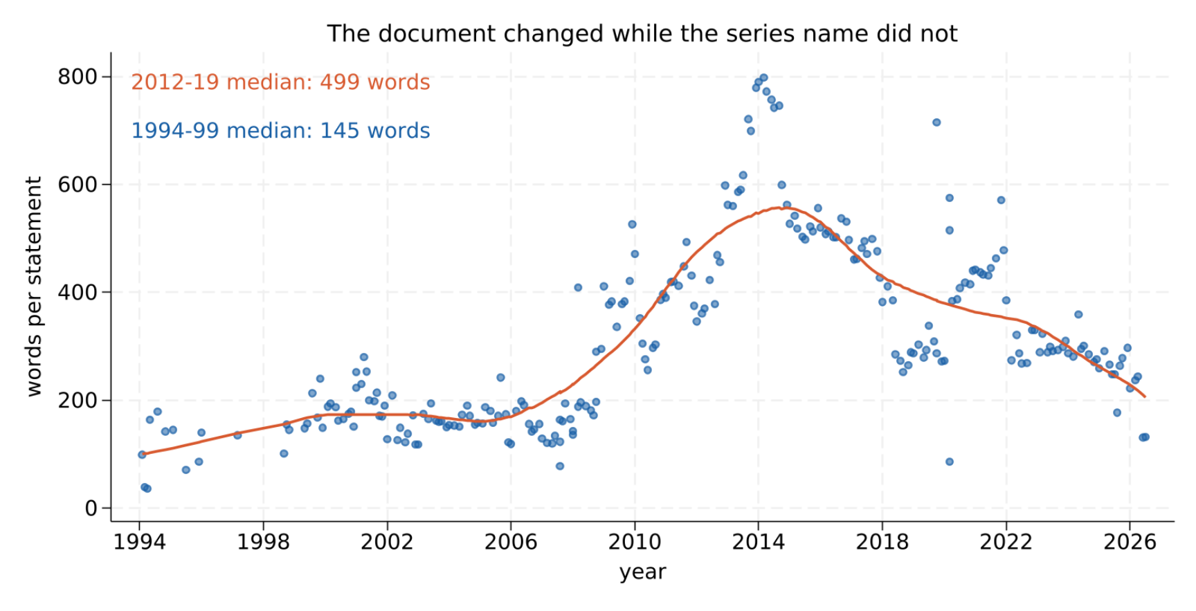
Before a single token is counted the corpus has already been chosen, and for the FOMC that choice is not innocent. Between 1994 and 1999 the Committee issued 20 statements in six years and 85% of them accompanied a change in the target rate: no change, no statement. From 2000 the statement became routine, and 226 of the 246 documents here come from that later regime — where only 19% of the 2012–2019 statements accompany a rate move.

The documents also changed shape. Median length runs 145 words in the 1990s, 499 in 2012–2019, then falls back to 294 from 2020.

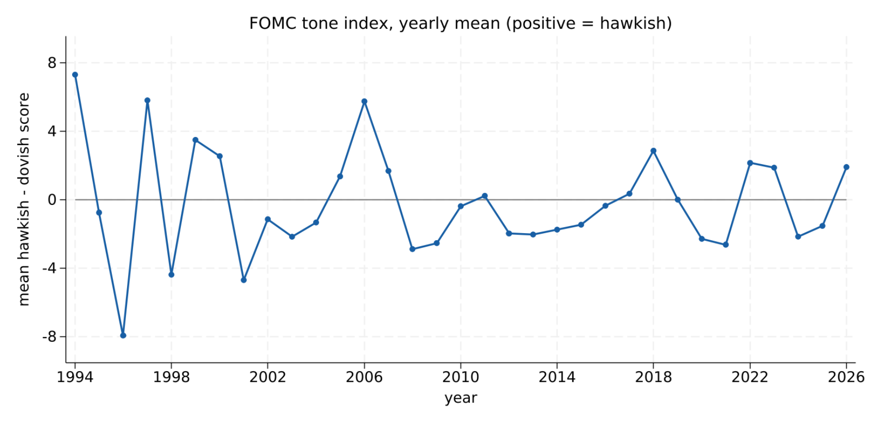
A tone index plotted from 1994 to 2026 therefore compares objects that are not the same object. Early statements exist because policy moved; later ones exist regardless. Any trend in such an index is partly a trend in what a statement is — and no amount of care downstream can undo it.

Code
fomc <- read.csv("../data/txt-fomc.csv")

# decimal year, so all three languages share one x axis
fomc <- fomc |>
  mutate(month = as.integer(format(as.Date(date), "%m"))) |>
  mutate(t = year + (month - 1) / 12)

# Cleveland lowess, single pass, so Stata's one-pass lowess matches exactly
sm  <- lowess(fomc$t, fomc$n_words, f = 0.30, iter = 0)
smd <- data.frame(t = sm$x, fit = sm$y)

ggplot(fomc) +
  aes(x = t, y = n_words) +
  geom_point(colour = "#185FA5", alpha = 0.55, size = 1.8) +
  geom_line(data = smd,
            mapping = aes(x = t, y = fit),
            colour = "#D85A30", linewidth = 1.1) +
  annotate("text", x = 1994.2, y = 700, hjust = 0, size = 4.2,
           colour = "#185FA5", label = "1994-99 median: 145 words") +
  annotate("text", x = 1994.2, y = 790, hjust = 0, size = 4.2,
           colour = "#D85A30", label = "2012-19 median: 499 words") +
  coord_cartesian(xlim = c(1993.5, 2027), ylim = c(0, 820)) +
  scale_x_continuous(breaks = seq(1994, 2026, 4)) +
  scale_y_continuous(breaks = seq(0, 800, 200)) +
  labs(x = "year", y = "words per statement",
       title = "The document changed while the series name did not")

Code
import pandas as pd
import matplotlib.pyplot as plt
from statsmodels.nonparametric.smoothers_lowess import lowess

fomc  = pd.read_csv("../data/txt-fomc.csv")
month = pd.to_datetime(fomc["date"]).dt.month
fomc  = fomc.assign(t=fomc["year"] + (month - 1) / 12)

# it=0 is the single-pass Cleveland lowess, matching R and Stata
sm = lowess(fomc["n_words"], fomc["t"], frac=0.30, it=0)

fig, ax = plt.subplots(figsize=(9, 4.6))
ax.plot(fomc["t"], fomc["n_words"], "o", color="#185FA5", alpha=0.55, markersize=4.2)
ax.plot(sm[:, 0], sm[:, 1], color="#D85A30", linewidth=2.0)
ax.text(1994.2, 700, "1994-99 median: 145 words", color="#185FA5", fontsize=11)
ax.text(1994.2, 790, "2012-19 median: 499 words",   color="#D85A30", fontsize=11)
axopts = ax.set(xlim=(1993.5, 2027), ylim=(0, 820),
                xticks=range(1994, 2027, 4), yticks=range(0, 801, 200),
                xlabel="year", ylabel="words per statement",
                title="The document changed while the series name did not")
plt.tight_layout()
plt.show()

Code
quietly import delimited "../data/txt-fomc.csv", clear varnames(1) ///
    bindquote(strict) maxquotedrows(unlimited)

* decimal year, so all three languages share one x axis
quietly gen int month = real(substr(date, 6, 2))
quietly gen double t  = year + (month - 1) / 12

* Stata's lowess is single pass, which is why R and Python set iter/it = 0
quietly lowess n_words t, bwidth(0.30) generate(fit) nograph

twoway (scatter n_words t, mcolor("24 95 165%55") msize(small))               ///
       (line fit t, sort lcolor("216 90 48") lwidth(medthick)),               ///
    legend(off)                                                               ///
    xscale(range(1993.5 2027)) xlabel(1994(4)2026)                            ///
    yscale(range(0 820)) ylabel(0(200)800)                                    ///
    xtitle("year") ytitle("words per statement")                              ///
    text(700 1994.2 "1994-99 median: 145 words", color("24 95 165") place(e)) ///
    text(790 1994.2 "2012-19 median: 499 words",   color("216 90 48") place(e)) ///
    title("The document changed while the series name did not", size(medium)) ///
    graphregion(color(white)) plotregion(color(white)) xsize(9) ysize(4.6)

graph export "../plots/txt-p1-comp.png", replace width(1600)

The Corpus, and What It Can Answer

246 FOMC statements, 4 February 1994 to 29 July 2026. The statement is the Committee’s only unanimous, simultaneous, on-the-record communication: released at a fixed instant, negotiated word by word, and known by everyone who writes it to be read as policy. That combination is rare, which is why this corpus recurs throughout the literature.

  • Public domain — a US Government work; no licence, no terms to accept
  • Complete — every statement ever issued, not a sample of them
  • Small — a median of 280.5 words, so LDA and embeddings run in seconds and the render stays honest
  • Precisely dated — to the minute, which is what makes event studies possible

The counterpart is that \(n = 246\) is genuinely small. Nothing here should be read as a claim that 246 documents support a deep model; the corpus is chosen so that every method can be run, inspected and broken in front of you.

Can answer — questions where the statement itself is the object of interest:

  • Does the language carry information beyond the rate decision it announces?
  • Does measured tone predict the next meeting’s decision, over and above the current one?
  • How has the composition of topics moved with the policy regime?

Cannot answer — anything needing variation the corpus does not contain:

  • The effect of communication on outcomes — 246 non-randomly-timed observations, every one endogenous
  • Individual disagreement — the statement is a committee product; use the transcripts, as Hansen, McMahon & Prat (2018) do
  • Anything about 1994–1999 tone trends, for the composition reason two slides back

This deck validates against the realized policy action, taken from the FRED target-rate series rather than from the text:

\[ \text{action}_i = \begin{cases} \text{hike} & \Delta \text{target}_i > 0 \\ \text{hold} & \Delta \text{target}_i = 0 \\ \text{cut} & \Delta \text{target}_i < 0 \end{cases} \]

giving 51 hikes, 155 holds and 40 cuts across the 246 meetings.

This is a deliberate substitution and it is stated rather than assumed. Most of the literature validates against hand-coded tone; the realized action is external to the text, verifiable and exactly reproducible — but it measures the decision, not the tone. Where the two diverge is itself informative, and Part 6 uses the next meeting’s action precisely because a model reading a statement that announces its own decision is not being asked anything hard.

Literature Review

  • Gentzkow, Kelly & Taddy (2019), “Text as Data”, JEL — the organising reference for this deck: representation, method, economics. doi:10.1257/jel.20181020
  • Ash & Hansen (2023), “Text Algorithms in Economics”, Annu. Rev. Econ. — the current map, method by method. doi:10.1146/annurev-economics-082222-074352
  • Dell (2025), “Deep Learning for Economists”, JEL — where embeddings and transformers now stand for applied work. doi:10.1257/jel.20241733
  • Kelly, Manela & Moreira (2021), “Text Selection”, JBES — the corpus is a sample, and selection into it is a modelling problem. doi:10.1080/07350015.2021.1947843
  • Hansen, McMahon & Prat (2018), QJE — LDA on FOMC transcripts; transparency changed how members spoke. doi:10.1093/qje/qjx045
  • Hansen & McMahon (2016), J. Int. Econ. — dictionary and topic measures of communication, with macroeconomic effects. doi:10.1016/j.jinteco.2015.12.008
  • Gorodnichenko, Pham & Talavera (2023), AER — the voice, not the words: tone of delivery moves markets. doi:10.1257/aer.20220129
  • Baker, Bloom & Davis (2016), QJE — the EPU index; the canonical newspaper-count economic variable. doi:10.1093/qje/qjw024
  • Loughran & McDonald (2011), J. Finance — why a general-purpose sentiment dictionary misreads financial text. doi:10.1111/j.1540-6261.2010.01625.x
  • Shapiro, Sudhof & Wilson (2022), J. Econometrics — building and validating a news sentiment series. doi:10.1016/j.jeconom.2020.07.053
  • Bybee, Kelly, Manela & Xiu (2024), J. Finance — topic shares from business news track the business cycle. doi:10.1111/jofi.13377
  • Hoberg & Phillips (2016), JPE — 10-K text as a similarity measure, and an industry classification built from it. doi:10.1086/688176
  • Pagan (1984), Int. Econ. Rev. — regressions with generated regressors. doi:10.2307/2648877
  • Murphy & Topel (1985), JBES — the two-step variance correction. doi:10.1080/07350015.1985.10509471
  • Clauset, Shalizi & Newman (2009), SIAM Review — the power-law test Part 2 applies to word frequencies. doi:10.1137/070710111
  • Ludwig, Mullainathan & Rambachan (2025), NBER wp 33344 — an econometric framework for treating an LLM as a measurement device. doi:10.3386/w33344

Part 2 — From Documents to Numbers

τὸ γὰρ βάρος νὼ βασανιεῖ τῶν ῥημάτων.

the weight of the words will put the two of us to the test

Ἀριστοφάνης, Βάτραχοι 1367

Tokenisation Is Already a Model

A tokeniser turns a string into a list of things to count. It sounds clerical. It is not: the token list defines the universe of possible findings, and nothing downstream can recover a distinction the tokeniser erased.

Take one real sentence from the corpus, 31 January 2024:

“In support of its goals, the Committee decided to maintain the target range for the federal funds rate at 5-1/4 to 5-1/2 percent.”

Each of these is a defensible answer to “what are the tokens?”, and they disagree about the most economically loaded item in the sentence:

  • Whitespace5-1/4 survives as one token, and so does percent. with its full stop
  • Letters only — the rate vanishes; the sentence is now about maintaining a target range
  • Alphanumeric5, 1, 4 appear as three separate meaningless tokens
  • Numeric-aware5.25 is retained as a number, and the sentence keeps its content

This deck uses the second rule — letters only. That choice deletes every interest rate from a corpus of interest-rate announcements, and it is still the right choice for this question, because the rate level is already in the data as the label. Had the question been “does the statement mention the rate?”, the same choice would have made it unanswerable.

Formally, tokenisation is a map from a string to a multiset of terms:

\[ \tau : \; \text{document } d_i \;\longmapsto\; \{\,t_{i1}, t_{i2}, \dots, t_{i m_i}\,\} \]

and the researcher chooses \(\tau\) through four settings. This deck’s choices, and what each one costs:

Decision This deck What it costs
Case lowercase everything Fed and fed merge; proper nouns are lost
Character class letters only every number, rate and date is deleted
Minimum length drop tokens of \(\le 2\) characters US, QE go with the noise
Splitting on whitespace hyphenated compounds split in two

The counts that build \(\mathbf{C}\) follow directly:

\[ c_{ij} \;=\; \sum_{k=1}^{m_i} \mathbb{1}\{\, t_{ik} = v_j \,\} \]

where \(v_j\) is the \(j\)-th entry of a vocabulary \(\mathcal{V} = \{v_1,\dots,v_p\}\) that has also been chosen. Two of those choices — the vocabulary and the weighting — get their own slides, because they matter more than the four above.

Stopwords, Stemming, Lemmatisation

Three operations reduce the vocabulary, and each is a claim about which distinctions do not matter.

  • Stopwords — delete terms carrying no information for this question. the and of are uncontroversial. Here committee, federal and percent are also stopwords, because they appear in essentially every statement and so cannot discriminate between them.
  • Stemming — chop suffixes by rule. inflation, inflationary, inflations all become inflat. Fast, crude, language-specific; the output is often not a word.
  • Lemmatisation — map to a dictionary head-word using a part-of-speech model. better becomes good. Linguistically correct, far slower, and it needs a model you did not estimate.

On this corpus the three choices move the vocabulary a long way:

Pipeline Distinct types
Nothing removed — every raw word 1,732
Stopwords removed, no stemming 1,602
Stopwords removed and Porter stemming 1,139
… then trimmed to terms in \(\ge 10\) documents 473

The last row is the one every later slide uses. Note its shape: 473 columns for 246 documents, so \(p > n\) before a single model has been fitted.

The Porter stemmer is a fixed sequence of rewrite rules keyed on a measure of syllable weight. Write a word as an alternation of consonant and vowel runs:

\[ [C]\,(VC)^{m}\,[V] \]

where \(m\) is the measure. Rules fire only when the stem’s measure clears a threshold, which is what stops tree becoming tr:

\[ (m > 0)\; \texttt{EED} \rightarrow \texttt{EE}, \qquad (m > 1)\; \texttt{EMENT} \rightarrow \varnothing \]

So agreed \(\rightarrow\) agree but feed \(\rightarrow\) feed; replacement \(\rightarrow\) replac while cement survives intact.

The algorithm is deterministic and has no parameters to estimate, so independent implementations mostly agree — R’s SnowballC, Python’s gensim and Stata’s txttool return the same stem for 1,716 of the 1,720 word types in this corpus, and produce an identical 473-term vocabulary. The four exceptions are on the last slide of this part, because they make the argument better than agreement would.

Stemming is not harmless for economics. Porter merges depress (the verb) with depression (the macroeconomic event), and separates stability from stabilisation. Whether that is a feature or a catastrophe depends entirely on the question, and no diagnostic will tell you which you got.

Three tokenisers with three default cleaning rules produce three different matrices, silently. This deck removes that risk by fixing three things.

1. The order is txttool’s, because Stata cannot reorder it and the other two can:

\[ \text{clean} \;\rightarrow\; \text{length filter} \;\rightarrow\; \text{stopwords} \;\rightarrow\; \text{Porter stem} \;\rightarrow\; \text{trim} \;\rightarrow\; \mathbf{C} \]

Order matters. Stemming before stopword removal would turn willing into will, and the stopword list would then delete both.

2. One stopword filetxt-stopwords.txt, 152 words, one per line, read unchanged by all three languages.

3. One vocabulary trim\(df_j \ge 10\), applied identically everywhere.

The parity check is displayed in every tab of the next slide: 473 terms, 24,291 non-zero cells, 38,477 tokens. R, Python and Stata reproduce all three exactly. If your three languages disagree, the pipeline is the first place to look — not the model.

Code — Build the Document-Term Matrix

Code
library(SnowballC)

fomc <- read.csv("../data/txt-fomc.csv")
stop <- readLines("../data/txt-stopwords.txt")

# clean -> length filter -> stopwords -> Porter stem, in that order
tokenise <- function(txt) {
  x <- gsub("[^a-z ]", " ", tolower(txt))
  w <- strsplit(x, "[[:space:]]+")[[1]]
  w <- w[nchar(w) > 2]
  w <- w[!(w %in% stop)]
  wordStem(w, language = "porter")
}

toks <- lapply(fomc$text, tokenise)

# document frequency, then the vocabulary trim
df    <- table(unlist(lapply(toks, unique)))
vocab <- sort(names(df)[df >= 10])
toks  <- lapply(toks, function(w) w[w %in% vocab])

# sparse triplets: one row per non-zero cell
trip <- do.call(rbind, lapply(seq_along(toks), function(i) {
  tb <- table(factor(toks[[i]], levels = vocab))
  tb <- tb[tb > 0]
  data.frame(doc_id = i, term = names(tb), count = as.integer(tb))
}))

cat(sprintf("documents  : %d\n", length(toks)))
cat(sprintf("vocabulary : %d terms (df >= 10)\n", length(vocab)))
cat(sprintf("triplets   : %d non-zero cells\n", nrow(trip)))
cat(sprintf("tokens     : %d\n", sum(trip$count)))
cat(sprintf("density    : %.4f\n", nrow(trip) / (length(toks) * length(vocab))))
documents  : 246
vocabulary : 473 terms (df >= 10)
triplets   : 24291 non-zero cells
tokens     : 38477
density    : 0.2088

top 8 terms by document frequency:
    term  df
    fund 236
  econom 235
  target 227
  inflat 217
   decid 214
  remain 214
  polici 209
 continu 207
Code
import re
import pandas as pd
from collections import Counter
from gensim.parsing.porter import PorterStemmer

fomc = pd.read_csv("../data/txt-fomc.csv")
stop = set(open("../data/txt-stopwords.txt").read().split())
ps   = PorterStemmer()

# clean -> length filter -> stopwords -> Porter stem, in that order
def tokenise(txt):
    w = re.sub(r"[^a-z ]", " ", txt.lower()).split()
    w = [x for x in w if len(x) > 2 and x not in stop]
    return [ps.stem(x) for x in w]

toks = [tokenise(t) for t in fomc["text"]]

# document frequency, then the vocabulary trim
df = Counter()
for d in toks:
    df.update(set(d))
vocab = sorted(t for t, c in df.items() if c >= 10)
keep  = set(vocab)
toks  = [[w for w in d if w in keep] for d in toks]

# sparse triplets: one row per non-zero cell
trip   = [(i, t, c) for i, d in enumerate(toks) for t, c in Counter(d).items()]
tokens = sum(c for row in trip for c in [row[2]])

out = (f"documents  : {len(toks)}\n"
       f"vocabulary : {len(vocab)} terms (df >= 10)\n"
       f"triplets   : {len(trip)} non-zero cells\n"
       f"tokens     : {tokens}\n"
       f"density    : {len(trip) / (len(toks) * len(vocab)):.4f}\n\n"
       "top 8 terms by document frequency:\n")
for t, c in sorted(((t, df[t]) for t in vocab), key=lambda z: -z[1])[:8]:
    out += f"  {t:<10} {c}\n"

import sys
nw = sys.stdout.write(out)
documents  : 246
vocabulary : 473 terms (df >= 10)
triplets   : 24291 non-zero cells
tokens     : 38477
density    : 0.2088

top 8 terms by document frequency:
  fund       236
  econom     235
  target     227
  inflat     217
  decid      214
  remain     214
  polici     209
  continu    207
Code
sys.stdout.flush()
Code
quietly import delimited "../data/txt-fomc.csv", clear varnames(1) ///
    bindquote(strict) maxquotedrows(unlimited)
quietly gen long doc_id = _n
keep doc_id text

* Clean, then hold ONE TOKEN PER OBSERVATION. A Stata string variable caps at
* 2,045 characters and these statements run to 5,456, so txttool cannot be
* shown a whole document. The long layout is also the sparse triplet form.
quietly replace text = ustrregexra(lower(text), "[^a-z]", " ")
quietly gen int nw = wordcount(text)
quietly expand nw
bysort doc_id: gen int k = _n
quietly gen str32 word = word(text, k)
drop text nw
quietly drop if strlen(word) <= 2

* Stem the VOCABULARY, not the corpus: txttool costs the same per row, and
* 1,700 distinct words sit behind 64,301 tokens - 0.9 seconds against 241.
preserve
    keep word
    quietly bysort word: keep if _n == 1
    quietly txttool word, stopwords("../data/txt-stopwords.txt") stem generate(term)
    tempfile stems
    quietly save `stems'
restore
quietly merge m:1 word using `stems', nogenerate
quietly drop if term == ""

* the document-term matrix in triplets, then the vocabulary trim
contract doc_id term, freq(count)
bysort term: gen int df = _N
quietly drop if df < 10

quietly egen byte tag = tag(term)
quietly count if tag
local V = r(N)
quietly summarize doc_id
local N = r(max)
quietly summarize count
local tokens = r(sum)
local trip = _N

display "documents  : " `N'
display "vocabulary : " `V' " terms (df >= 10)"
display "triplets   : " `trip' " non-zero cells"
display "tokens     : " `tokens'
display "density    : " %6.4f `trip' / (`N' * `V')

display _newline "top 8 terms by document frequency:"
quietly keep if tag
gsort -df term
list term df in 1/8, noobs clean
documents  : 246

vocabulary : 473 terms (df >= 10)

triplets   : 24291 non-zero cells

tokens     : 38477

density    : 0.2088


top 8 terms by document frequency:

       term    df  
       fund   236  
     econom   235  
     target   227  
     inflat   217  
      decid   214  
     remain   214  
     polici   209  
    continu   207  

What Bigrams Buy, and What They Cost

A unigram model treats a document as an unordered bag: “inflation is falling” and “falling is inflation” have identical representations. Bigrams — adjacent pairs — restore a slice of word order:

\[ \text{bigrams}(d_i) = \bigl\{\, (t_{ik},\, t_{i,k+1}) \,\bigr\}_{k=1}^{m_i - 1} \]

What they buy. Phrases whose meaning is not the sum of their parts, and which happen to be the interesting objects in policy language: price_stabil, maximum_employ, inflat_expect, target_rang.

What they cost. Dimension, brutally. With \(p\) unigrams there are up to \(p^2\) ordered pairs:

\[ p = 473 \;\Longrightarrow\; p^2 = 223{,}729 \text{ possible bigrams}, \qquad n = 246 \text{ documents} \]

In practice this corpus yields 7,132 distinct bigrams from 40,469 bigram tokens — so most appear once or twice, and the vocabulary must be trimmed harder than the unigram one. At a threshold of 10 occurrences, 908 survive.

Stopword removal manufactures adjacencies that never existed. Two of the top bigrams opposite are artefacts: labor_condit comes from “labor market conditions” and rang_fund from “range for the federal funds rate”. If phrases matter to your question, form bigrams before deleting stopwords — or accept that some of them are fictional.

Code
library(SnowballC)

fomc <- read.csv("../data/txt-fomc.csv")
stop <- readLines("../data/txt-stopwords.txt")

# the stemmed, stopworded stream - NOT trimmed to the 473-term vocabulary,
# because a bigram of two kept terms is not the same as a kept bigram
tokenise <- function(txt) {
  w <- strsplit(gsub("[^a-z ]", " ", tolower(txt)), "[[:space:]]+")[[1]]
  w <- w[nchar(w) > 2]
  wordStem(w[!(w %in% stop)], language = "porter")
}
toks <- lapply(fomc$text, tokenise)

bigrams <- unlist(lapply(toks, function(w) {
  if (length(w) < 2) return(character(0))
  paste(w[-length(w)], w[-1], sep = "_")
}))

tb <- sort(table(bigrams), decreasing = TRUE)

cat(sprintf("bigram tokens    : %d\n", length(bigrams)))
cat(sprintf("distinct bigrams : %d\n", length(tb)))
cat(sprintf("surviving n >= 10: %d\n", sum(tb >= 10)))
cat("\ntop 8 bigrams:\n")
print(data.frame(bigram = names(head(tb, 8)),
                 count  = as.integer(head(tb, 8))), row.names = FALSE)
bigram tokens    : 40469
distinct bigrams : 7132
surviving n >= 10: 908

top 8 bigrams:
          bigram count
 monetari_polici   294
  maximum_employ   293
   inflat_expect   292
    econom_activ   281
     target_rang   277
    price_stabil   270
    labor_condit   262
       rang_fund   237
Code
import re
import pandas as pd
from collections import Counter
from gensim.parsing.porter import PorterStemmer

fomc = pd.read_csv("../data/txt-fomc.csv")
stop = set(open("../data/txt-stopwords.txt").read().split())
ps   = PorterStemmer()

# the stemmed, stopworded stream - NOT trimmed to the 473-term vocabulary,
# because a bigram of two kept terms is not the same as a kept bigram
def tokenise(txt):
    w = re.sub(r"[^a-z ]", " ", txt.lower()).split()
    return [ps.stem(x) for x in w if len(x) > 2 and x not in stop]

btoks = [tokenise(t) for t in fomc["text"]]

bigrams = [f"{d[k]}_{d[k + 1]}" for d in btoks for k in range(len(d) - 1)]
tb = Counter(bigrams)

out = (f"bigram tokens    : {len(bigrams)}\n"
       f"distinct bigrams : {len(tb)}\n"
       f"surviving n >= 10: {sum(1 for c in tb.values() if c >= 10)}\n\n"
       "top 8 bigrams:\n")
for b, c in tb.most_common(8):
    out += f"  {b:<18} {c}\n"

import sys
nw = sys.stdout.write(out)
bigram tokens    : 40469
distinct bigrams : 7132
surviving n >= 10: 908

top 8 bigrams:
  monetari_polici    294
  maximum_employ     293
  inflat_expect      292
  econom_activ       281
  target_rang        277
  price_stabil       270
  labor_condit       262
  rang_fund          237
Code
sys.stdout.flush()
Code
quietly import delimited "../data/txt-fomc.csv", clear varnames(1) ///
    bindquote(strict) maxquotedrows(unlimited)
quietly gen long doc_id = _n
keep doc_id text
quietly replace text = ustrregexra(lower(text), "[^a-z]", " ")
quietly gen int nw = wordcount(text)
quietly expand nw
bysort doc_id: gen int k = _n
quietly gen str32 word = word(text, k)
drop text nw
quietly drop if strlen(word) <= 2

preserve
    keep word
    quietly bysort word: keep if _n == 1
    quietly txttool word, stopwords("../data/txt-stopwords.txt") stem generate(term)
    tempfile stems
    quietly save `stems'
restore
quietly merge m:1 word using `stems', nogenerate
quietly drop if term == ""

* one row per token in reading order, so a bigram is just the next row's stem
sort doc_id k
quietly by doc_id: gen str64 bigram = term + "_" + term[_n + 1] if _n < _N
quietly drop if missing(bigram)
local btokens = _N

contract bigram, freq(count)
local distinct = _N
quietly count if count >= 10
local surviving = r(N)

display "bigram tokens    : " `btokens'
display "distinct bigrams : " `distinct'
display "surviving n >= 10: " `surviving'

display _newline "top 8 bigrams:"
gsort -count bigram
list bigram count in 1/8, noobs clean
bigram tokens    : 40469

distinct bigrams : 7132

surviving n >= 10: 908


top 8 bigrams:

             bigram   count  
    monetari_polici     294  
     maximum_employ     293  
      inflat_expect     292  
       econom_activ     281  
        target_rang     277  
       price_stabil     270  
       labor_condit     262  
          rang_fund     237  

The Matrix: Sparsity and tf-idf

The trimmed matrix is \(246 \times 473\), which is 116,358 cells. Only 24,291 are non-zero:

\[ \text{density} = \frac{24{,}291}{246 \times 473} = 0.209, \qquad \text{so } 79.1\% \text{ of the matrix is zero} \]

And this is a dense text matrix, because the vocabulary was trimmed hard. An untrimmed corpus is routinely 99.9% zeros.

Two consequences, one computational and one statistical.

  • Store triplets, not the matrix. Keeping \((i, j, c_{ij})\) for non-zero cells only costs 24,291 rows instead of 116,358, and the saving grows with the corpus. Every language here reads the DTM in that form.
  • A zero is not a measurement of zero. \(c_{ij} = 0\) conflates “this document is not about that” with “the document was too short to mention it”. Document length is therefore a confounder in every count model, and normalising by it is not optional.

Raw counts give the most weight to the terms that discriminate least. tf-idf rescales each cell by how rare the term is across documents:

\[ \text{tf-idf}_{ij} \;=\; \underbrace{\frac{c_{ij}}{\sum_{j'} c_{ij'}}}_{\text{term frequency}} \times \underbrace{\log\!\left(\frac{n}{df_j}\right)}_{\text{inverse document frequency}} \]

where \(df_j\) is the number of documents containing term \(j\). The first factor removes document length; the second down-weights ubiquity. In this corpus the idf factor spans

\[ \log\!\left(\frac{246}{236}\right) = 0.041 \qquad\text{to}\qquad \log\!\left(\frac{246}{10}\right) = 3.203 \]

so fund, in 236 of the 246 statements, is weighted about 77 times less than a term appearing in the minimum 10.

tf-idf is a modelling assumption wearing the clothes of a normalisation. It asserts that informativeness is inversely proportional to log document frequency — a heuristic from information retrieval, where the goal was ranking documents for a human reader, not estimating a parameter. It has no derivation from any economic or statistical model. A supervised method, in Part 3, learns the weights rather than assuming them.

Zipf’s Law, and Testing It Properly

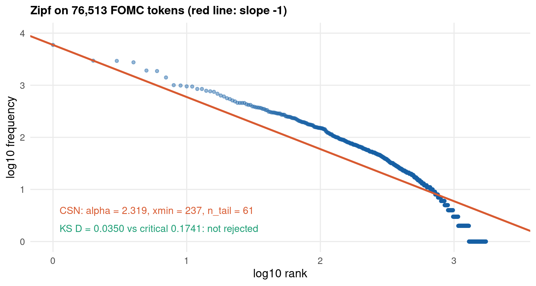
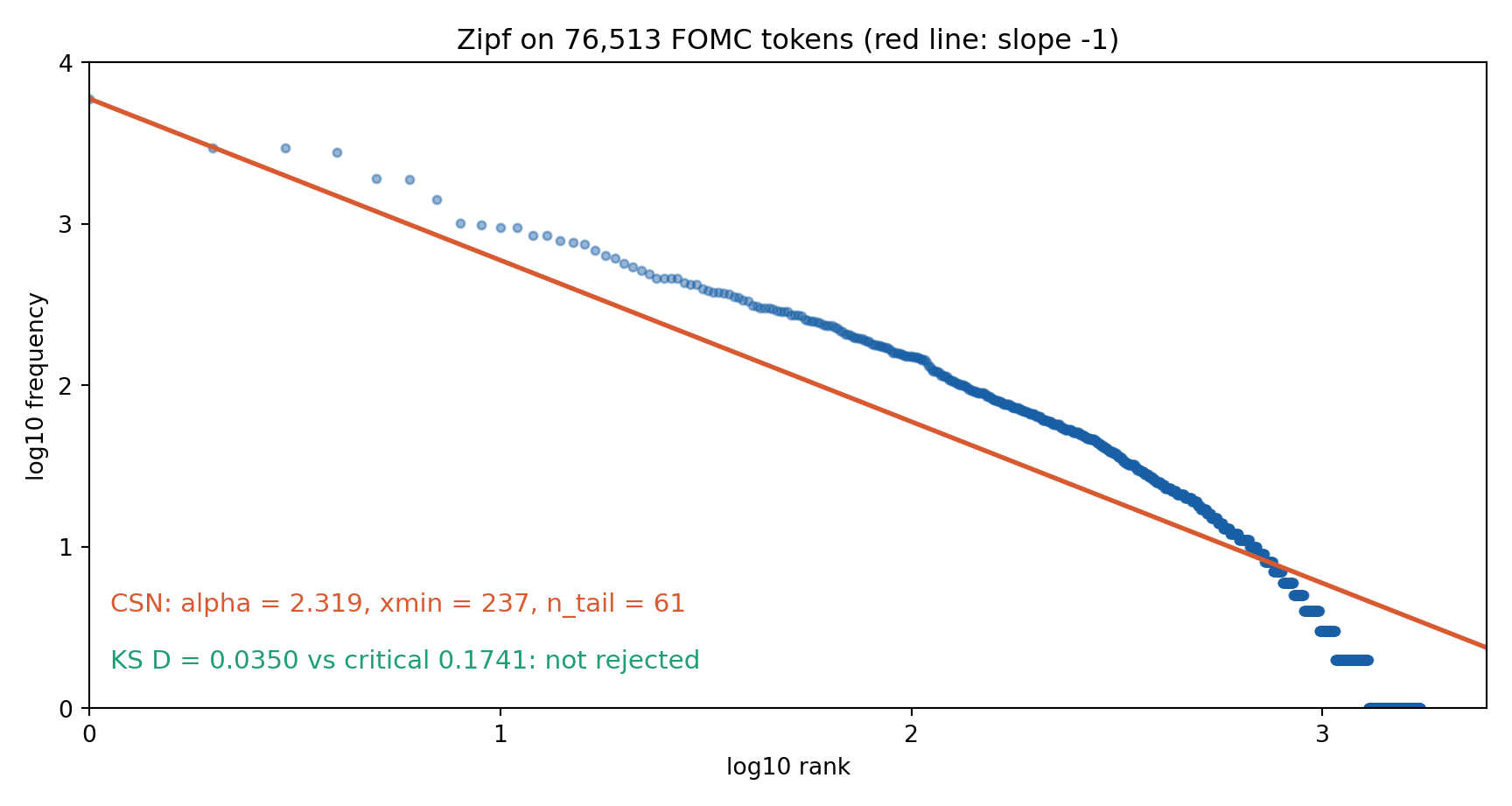
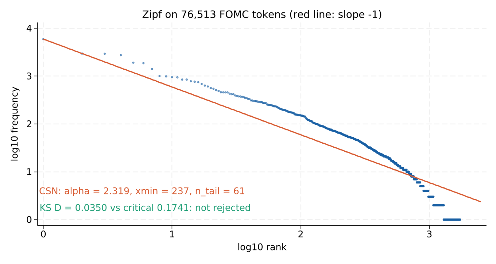
Rank the words of any natural-language corpus by frequency. The \(r\)-th most common occurs roughly \(1/r\) times as often as the first. Across all 76,513 raw tokens and 1,732 distinct words here:

Rank Word Count
1 the 5,942
2 to 2,962
3 and 2,934
4 of 2,753
5 committee 1,915

At the other end, 440 words — 25.4% of the vocabulary — occur exactly once. That is the hapax legomena problem, and it is why a text design matrix cannot be treated like a survey design matrix: a quarter of your columns have a single non-zero entry.

This matters well beyond a curiosity about language:

  • It is why vocabulary trimming is unavoidable rather than optional
  • It is why raw counts need weighting — otherwise a handful of terms dominate every distance and every regression
  • It is why adding documents adds new terms almost linearly, so \(p\) grows with \(n\) and the asymptotics you learned do not apply

Zipf’s law relates rank \(r\) to frequency \(f\):

\[ f(r) \;\propto\; r^{-s}, \qquad s \approx 1 \]

The equivalent statement about the distribution of frequencies is a power law:

\[ \Pr(F \ge f) \;\propto\; f^{-(\alpha - 1)}, \qquad \alpha \;=\; 1 + \frac{1}{s} \]

so Zipf’s \(s = 1\) corresponds to \(\alpha = 2\).

Do not fit this by regressing \(\log f\) on \(\log r\). It is standard practice and it is biased: the points are not independent, the errors are not Gaussian in logs, and \(R^2\) on a log-log plot is high for distributions that are not power laws at all. Clauset, Shalizi & Newman (2009) give the correct procedure, reused here from Networks and Trade Analysis:

  1. For each candidate \(x_{\min}\), fit the tail by maximum likelihood \[ \hat\alpha(x_{\min}) \;=\; 1 + n_{\text{tail}} \left[ \sum_{f_i \ge x_{\min}} \ln \frac{f_i}{x_{\min}} \right]^{-1} \]
  2. Measure fit by the Kolmogorov–Smirnov distance between empirical and fitted CDFs \[ D(x_{\min}) \;=\; \max_{f \ge x_{\min}} \bigl| \, \hat{F}_{\text{emp}}(f) - F_{\text{fit}}(f) \, \bigr| \]
  3. Take the \(x_{\min}\) that minimises \(D\), and judge against \(1.36/\sqrt{n_{\text{tail}}}\)

On this corpus the procedure selects \(x_{\min} = 237\), leaving \(n_{\text{tail}} = 61\) word types, and returns

\[ \hat\alpha = 2.319, \qquad D = 0.0350, \qquad 1.36/\sqrt{61} = 0.1741 \]

so the power law is not rejected. Note what \(\hat\alpha = 2.319\) implies for Zipf: \(s = 1/(\hat\alpha - 1) = 0.76\), flatter than the textbook \(s = 1\).

With \(n_{\text{tail}}\) in the dozens this test has very little power: not rejected is weak evidence, exactly as in the networks deck. It is shown here to teach the procedure — and to make the point that the log-log line everyone plots is not a test.

Code — Zipf and the CSN Test

Code
fomc <- read.csv("../data/txt-fomc.csv")

# raw words: no stopwords, no stemming - Zipf is about words, not stems
all  <- paste(fomc$text, collapse = " ")
w    <- strsplit(gsub("[^a-z ]", " ", tolower(all)), "[[:space:]]+")[[1]]
w    <- w[nchar(w) > 0]
freq <- sort(as.integer(table(w)), decreasing = TRUE)

# CSN: x_min minimises the KS distance, alpha is ML on the tail
csn <- function(x) {
  best <- NULL
  for (xm in sort(unique(x[x >= 2]))) {
    tl <- sort(x[x >= xm])
    nt <- length(tl)
    if (nt < 50) next
    al <- 1 + nt / sum(log(tl / xm))
    D  <- max(abs((seq_len(nt) - 0.5) / nt - (1 - (tl / xm)^(1 - al))))
    if (is.null(best) || D < best$D)
      best <- list(xmin = xm, alpha = al, D = D, n = nt)
  }
  best
}
fit  <- csn(freq)
crit <- 1.36 / sqrt(fit$n)

zp <- data.frame(rank = seq_along(freq), freq = freq)

ggplot(zp) +
  aes(x = log10(rank), y = log10(freq)) +
  geom_point(colour = "#185FA5", alpha = 0.45, size = 1.5) +
  geom_abline(intercept = log10(freq[1]), slope = -1,
              colour = "#D85A30", linewidth = 1.1) +
  annotate("text", x = 0.05, y = 0.60, hjust = 0, size = 4.2, colour = "#D85A30",
           label = sprintf("CSN: alpha = %.3f, xmin = %d, n_tail = %d",
                           fit$alpha, fit$xmin, fit$n)) +
  annotate("text", x = 0.05, y = 0.25, hjust = 0, size = 4.2, colour = "#1D9E75",
           label = sprintf("KS D = %.4f vs critical %.4f: not rejected",
                           fit$D, crit)) +
  coord_cartesian(xlim = c(0, 3.4), ylim = c(0, 4)) +
  scale_x_continuous(breaks = 0:3) +
  scale_y_continuous(breaks = 0:4) +
  labs(x = "log10 rank", y = "log10 frequency",
       title = "Zipf on 76,513 FOMC tokens (red line: slope -1)")

Code
import re
import numpy as np
import pandas as pd
import matplotlib.pyplot as plt
from collections import Counter

fomc = pd.read_csv("../data/txt-fomc.csv")

# raw words: no stopwords, no stemming - Zipf is about words, not stems
allw = re.sub(r"[^a-z ]", " ", " ".join(fomc["text"]).lower()).split()
freq = np.array(sorted(Counter(allw).values()))[::-1]

# CSN: x_min minimises the KS distance, alpha is ML on the tail
def csn(x):
    best = None
    for xm in np.unique(x[x >= 2]):
        tl = np.sort(x[x >= xm])
        nt = len(tl)
        if nt < 50:
            continue
        al = 1 + nt / np.sum(np.log(tl / xm))
        D  = np.max(np.abs((np.arange(1, nt + 1) - 0.5) / nt
                           - (1 - (tl / xm) ** (1 - al))))
        if best is None or D < best[2]:
            best = (xm, al, D, nt)
    return best

xmin, alpha, D, ntail = csn(freq)
crit = 1.36 / np.sqrt(ntail)
rank = np.arange(1, len(freq) + 1)

fig, ax = plt.subplots(figsize=(9, 4.8))
ax.plot(np.log10(rank), np.log10(freq), "o", color="#185FA5", alpha=0.45, markersize=3.5)
ax.plot([0, 3.4], [np.log10(freq[0]), np.log10(freq[0]) - 3.4],
        color="#D85A30", linewidth=2.0)
# the numbers ride on the figure: a Python chunk that draws also loses stdout
ax.text(0.05, 0.60, f"CSN: alpha = {alpha:.3f}, xmin = {xmin}, n_tail = {ntail}",
        color="#D85A30", fontsize=11)
ax.text(0.05, 0.25, f"KS D = {D:.4f} vs critical {crit:.4f}: not rejected",
        color="#1D9E75", fontsize=11)
axopts = ax.set(xlim=(0, 3.4), ylim=(0, 4), xticks=range(0, 4), yticks=range(0, 5),
                xlabel="log10 rank", ylabel="log10 frequency",
                title="Zipf on 76,513 FOMC tokens (red line: slope -1)")
plt.tight_layout()
plt.show()

Code
quietly import delimited "../data/txt-fomc.csv", clear varnames(1) ///
    bindquote(strict) maxquotedrows(unlimited)
keep text
quietly replace text = ustrregexra(lower(text), "[^a-z]", " ")
quietly gen long doc_id = _n
quietly gen int nw = wordcount(text)
quietly expand nw
bysort doc_id: gen int k = _n
quietly gen str32 word = word(text, k)
keep word
quietly drop if word == ""

* raw words: no stopwords, no stemming - Zipf is about words, not stems
contract word, freq(freq)
gsort -freq word
quietly gen long rank = _n
quietly gen double lr = log10(rank)
quietly gen double lf = log10(freq)
local top = lf[1]

* CSN: x_min minimises the KS distance, alpha is ML on the tail
quietly levelsof freq if freq >= 2, local(cands)
local bestD = 99
foreach xm of local cands {
    quietly count if freq >= `xm'
    local nt = r(N)
    if `nt' >= 50 {
        preserve
            quietly keep if freq >= `xm'
            sort freq
            quietly gen double lg = log(freq / `xm')
            quietly summarize lg, meanonly
            local al = 1 + `nt' / r(sum)
            quietly gen double emp = (_n - 0.5) / `nt'
            quietly gen double th  = 1 - (freq / `xm')^(1 - `al')
            quietly gen double ad  = abs(emp - th)
            quietly summarize ad, meanonly
            local D = r(max)
        restore
        if `D' < `bestD' {
            local bestD = `D'
            local bestA = `al'
            local bestX = `xm'
            local bestN = `nt'
        }
    }
}
local crit = 1.36 / sqrt(`bestN')
local lab1 = "CSN: alpha = " + string(`bestA', "%5.3f") + ", xmin = " ///
           + string(`bestX') + ", n_tail = " + string(`bestN')
local lab2 = "KS D = " + string(`bestD', "%6.4f") + " vs critical " ///
           + string(`crit', "%6.4f") + ": not rejected"

twoway (scatter lf lr, mcolor("24 95 165%45") msize(vsmall))                   ///
       (function y = `top' - x, range(0 3.4) lcolor("216 90 48") lwidth(medthick)), ///
    legend(off)                                                                ///
    xscale(range(0 3.4)) xlabel(0(1)3) yscale(range(0 4)) ylabel(0(1)4)         ///
    xtitle("log10 rank") ytitle("log10 frequency")                             ///
    text(0.60 0.05 "`lab1'", color("216 90 48") place(e))                      ///
    text(0.25 0.05 "`lab2'", color("29 158 117") place(e))                     ///
    title("Zipf on 76,513 FOMC tokens (red line: slope -1)", size(medium))     ///
    graphregion(color(white)) plotregion(color(white)) xsize(9) ysize(4.8)

graph export "../plots/txt-p2-zipf.png", replace width(1600)

Preprocessing Sensitivity

The honest way to report a preprocessing choice is to show what happens under the alternatives. Four pipelines, all defensible, all common in published work:

# Pipeline
A stopwords removed, Porter stemming, tokens of \(\ge 3\) characters
B stopwords removed, no stemming
C Porter stemming, no stopword removal
D no stopwords, length filter relaxed to \(\ge 2\) characters

Each produces a tone score for every statement,

\[ \text{tone}_i \;=\; 100 \times \frac{\#\{\text{hawkish terms}\} - \#\{\text{dovish terms}\}}{\#\{\text{tokens}\}} \]

which is standardised and used to predict whether the next meeting hikes:

\[ \Pr\bigl(\text{hike}_{i+1} = 1\bigr) \;=\; \Lambda\bigl(\beta_0 + \beta_1 \, \widetilde{\text{tone}}_i\bigr) \]

The answer is more precise — and more useful — than “preprocessing changes everything”.

The sign and the significance are robust. All four pipelines give a positive coefficient with \(t\) between \(4.87\) and \(5.77\). The documents also rank almost identically: Spearman correlations between pipelines run from \(0.961\) to \(1.000\).

The magnitude and the level are not. The coefficient spans \(0.886\) to \(1.159\) — a range of about 1.4 standard errors, wider than most published robustness checks. And the mean of the index moves from \(-0.450\) to \(-0.175\), a factor of \(2.6\), because the denominator changes with the pipeline.

So: if the estimand is the sign of a coefficient on a standardised index, you are probably safe. If it is a magnitude, a threshold, a level, or a comparison between corpora, the pipeline is doing real work and belongs in the specification table like any other choice.

One number in the table below is not identical across languages, and that is the point. Three implementations all called “Porter” disagree on 4 of the 1,720 word types here: R’s SnowballC stems as and is to a and i, and technology to technologi, where gensim and txttool leave as and is alone and give technolog. On this corpus the disagreements happen to cancel in the type count, and technology appears in 2 documents — far below the \(df \ge 10\) cut — so the 473-term vocabulary and every displayed figure agree exactly. They need not have: an undocumented implementation detail sits one word away from moving a reported number, which is the argument of this part in miniature.

Code
library(SnowballC)

fomc <- read.csv("../data/txt-fomc.csv")
lab  <- read.csv("../data/txt-labels.csv")
stop <- readLines("../data/txt-stopwords.txt")
dict <- read.csv("../data/txt-dict.csv")

hawk <- dict$word[dict$category == "hawkish"]
dove <- dict$word[dict$category == "dovish"]

# one pipeline: three switches, applied in the fixed order
pipe <- function(txt, use_stop, use_stem, minlen) {
  w <- strsplit(gsub("[^a-z ]", " ", tolower(txt)), "[[:space:]]+")[[1]]
  w <- w[nchar(w) >= minlen]
  if (use_stop) w <- w[!(w %in% stop)]
  if (use_stem) w <- wordStem(w, language = "porter")
  w[nchar(w) > 0]          # Porter maps some 1-character tokens to ""
}

tone <- function(use_stop, use_stem, minlen) {
  H <- if (use_stem) unique(wordStem(hawk, "porter")) else hawk
  D <- if (use_stem) unique(wordStem(dove, "porter")) else dove
  sapply(fomc$text, function(t) {
    w <- pipe(t, use_stop, use_stem, minlen)
    100 * (sum(w %in% H) - sum(w %in% D)) / length(w)
  })
}

cfg <- list(A = c(1, 1, 3), B = c(1, 0, 3), C = c(0, 1, 3), D = c(0, 1, 2))
y   <- as.integer(lab$next_action == "hike")
ok  <- !is.na(y)

res <- data.frame()
for (nm in names(cfg)) {
  a <- cfg[[nm]]
  z <- tone(a[1] == 1, a[2] == 1, a[3])
  m <- summary(glm(y[ok] ~ scale(z)[ok], family = binomial))$coefficients[2, ]
  types <- length(unique(unlist(lapply(fomc$text, pipe,
             use_stop = a[1] == 1, use_stem = a[2] == 1, minlen = a[3]))))
  res <- rbind(res, data.frame(pipeline = nm, types = types,
                               mean_tone = round(mean(z), 3),
                               coef = round(m[1], 4), t = round(m[3], 3)))
}
print(res, row.names = FALSE)
 pipeline types mean_tone   coef     t
        A  1139    -0.286 1.1510 5.714
        B  1602    -0.450 0.8864 4.871
        C  1225    -0.202 1.1590 5.752
        D  1241    -0.175 1.1545 5.773

Spearman correlation between pipelines:
      A     B     C     D
A 1.000 0.961 0.999 0.999
B 0.961 1.000 0.962 0.962
C 0.999 0.962 1.000 1.000
D 0.999 0.962 1.000 1.000
Code
import re
import numpy as np
import pandas as pd
import statsmodels.api as sm
from scipy.stats import spearmanr
from gensim.parsing.porter import PorterStemmer

fomc = pd.read_csv("../data/txt-fomc.csv")
lab  = pd.read_csv("../data/txt-labels.csv")
stop = set(open("../data/txt-stopwords.txt").read().split())
dic  = pd.read_csv("../data/txt-dict.csv")
ps   = PorterStemmer()

hawk = list(dic.loc[dic["category"] == "hawkish", "word"])
dove = list(dic.loc[dic["category"] == "dovish",  "word"])

# one pipeline: three switches, applied in the fixed order
def pipe(txt, use_stop, use_stem, minlen):
    w = re.sub(r"[^a-z ]", " ", txt.lower()).split()
    w = [x for x in w if len(x) >= minlen]
    if use_stop:
        w = [x for x in w if x not in stop]
    if use_stem:
        w = [ps.stem(x) for x in w]
    return [x for x in w if x]   # Porter maps some 1-character tokens to ""

def tone(use_stop, use_stem, minlen):
    H = set(ps.stem(x) for x in hawk) if use_stem else set(hawk)
    D = set(ps.stem(x) for x in dove) if use_stem else set(dove)
    vals = []
    for t in fomc["text"]:
        w = pipe(t, use_stop, use_stem, minlen)
        vals.append(100 * (sum(x in H for x in w) - sum(x in D for x in w)) / len(w))
    return np.array(vals)

cfg = {"A": (1, 1, 3), "B": (1, 0, 3), "C": (0, 1, 3), "D": (0, 1, 2)}
y   = (lab["next_action"] == "hike").astype(float).values
ok  = lab["next_action"].notna().values

rows, zz = [], {}
for nm, (us, ust, ml) in cfg.items():
    z  = tone(us == 1, ust == 1, ml)
    zz[nm] = z
    zs = (z - z.mean()) / z.std(ddof=1)
    fit = sm.Logit(y[ok], sm.add_constant(zs[ok])).fit(disp=0)
    types = len(set(x for t in fomc["text"] for x in pipe(t, us == 1, ust == 1, ml)))
    rows.append((nm, types, z.mean(), fit.params[1], fit.tvalues[1]))

out = f"{'pipeline':<10}{'types':>7}{'mean_tone':>11}{'coef':>10}{'t':>9}\n"
for nm, ty, mt, cf, tv in rows:
    out += f"{nm:<10}{ty:>7}{mt:>11.3f}{cf:>10.4f}{tv:>9.3f}\n"
out += "\nSpearman correlation between pipelines:\n" + " " * 10
ks = list(cfg)
out += "".join(f"{k:>8}" for k in ks) + "\n"
for a in ks:
    out += f"{a:<10}" + "".join(f"{spearmanr(zz[a], zz[b]).statistic:>8.3f}" for b in ks) + "\n"

import sys
nw = sys.stdout.write(out)
pipeline    types  mean_tone      coef        t
A            1139     -0.286    1.1510    5.714
B            1602     -0.450    0.8864    4.871
C            1225     -0.202    1.1590    5.752
D            1241     -0.175    1.1545    5.773

Spearman correlation between pipelines:
                 A       B       C       D
A            1.000   0.961   0.999   0.999
B            0.961   1.000   0.962   0.962
C            0.999   0.962   1.000   1.000
D            0.999   0.962   1.000   1.000
Code
sys.stdout.flush()
Code
* Build ONE long token table carrying everything the four pipelines need: the
* raw word, its Porter stem, its length, whether it is a stopword and whether
* it is a dictionary term. Each pipeline is then a filter over that table, so
* txttool runs once instead of four times.
quietly import delimited "../data/txt-fomc.csv", clear varnames(1) ///
    bindquote(strict) maxquotedrows(unlimited)
quietly gen long doc_id = _n
keep doc_id text
quietly replace text = ustrregexra(lower(text), "[^a-z]", " ")
quietly gen int nw = wordcount(text)
quietly expand nw
bysort doc_id: gen int k = _n
quietly gen str32 word = word(text, k)
drop text nw
quietly drop if word == ""
quietly gen int len = strlen(word)

preserve
    keep word
    quietly bysort word: keep if _n == 1
    quietly txttool word, stem generate(stem)
    tempfile stems
    quietly save `stems'
restore
quietly merge m:1 word using `stems', nogenerate

preserve
    quietly import delimited "../data/txt-stopwords.txt", clear varnames(nonames)
    quietly rename v1 word
    quietly gen byte is_stop = 1
    tempfile sw
    quietly save `sw'
restore
quietly merge m:1 word using `sw', nogenerate keep(master match)
quietly replace is_stop = 0 if missing(is_stop)

* the policy dictionary, in raw and stemmed form
preserve
    quietly import delimited "../data/txt-dict.csv", clear varnames(1)
    quietly keep if category == "hawkish" | category == "dovish"
    quietly gen byte hawk = category == "hawkish"
    keep word hawk
    quietly bysort word: keep if _n == 1
    tempfile draw
    quietly save `draw'
    quietly txttool word, stem replace
    quietly rename word stem
    quietly bysort stem: keep if _n == 1
    tempfile dstem
    quietly save `dstem'
restore
quietly merge m:1 word using `draw', nogenerate keep(master match) keepusing(hawk)
quietly rename hawk hawk_raw
quietly merge m:1 stem using `dstem', nogenerate keep(master match) keepusing(hawk)
quietly rename hawk hawk_stem
tempfile tokens
quietly save `tokens'

preserve
    quietly import delimited "../data/txt-labels.csv", clear varnames(1)
    quietly gen long doc_id = _n
    quietly gen byte y = next_action == "hike"
    quietly replace y = . if !inlist(next_action, "hike", "hold", "cut")
    keep doc_id y
    tempfile lab
    quietly save `lab'
restore

display "pipeline    types   mean_tone       coef         t"
foreach spec in "A 1 1 3" "B 1 0 3" "C 0 1 3" "D 0 1 2" {
    local nm  : word 1 of `spec'
    local us  : word 2 of `spec'
    local ust : word 3 of `spec'
    local ml  : word 4 of `spec'

    quietly use `tokens', clear
    quietly drop if len < `ml'
    if `us' == 1 quietly drop if is_stop == 1

    if `ust' == 1 {
        quietly gen str32 tok  = stem
        quietly gen byte hawkf = hawk_stem == 1
        quietly gen byte dovef = hawk_stem == 0
    }
    else {
        quietly gen str32 tok  = word
        quietly gen byte hawkf = hawk_raw == 1
        quietly gen byte dovef = hawk_raw == 0
    }
    quietly drop if tok == ""
    quietly egen byte tagt = tag(tok)
    quietly count if tagt
    local types = r(N)

    quietly collapse (sum) hawkf dovef (count) ntok = len, by(doc_id)
    quietly gen double tone = 100 * (hawkf - dovef) / ntok
    quietly summarize tone
    local mt = r(mean)
    local sd = r(sd)
    quietly gen double ztone = (tone - `mt') / `sd'

    quietly merge 1:1 doc_id using `lab', nogenerate
    quietly logit y ztone
    local cf = _b[ztone]
    local tv = _b[ztone] / _se[ztone]

    display "`nm'" _col(10) %8.0f `types' _col(21) %10.3f `mt' ///
            _col(32) %10.4f `cf' _col(43) %9.3f `tv'
}
pipeline    types   mean_tone       coef         t

 34. }
A            1139       -0.286     1.1510     5.714
B            1602       -0.450     0.8864     4.871
C            1225       -0.202     1.1590     5.752
D            1241       -0.175     1.1545     5.773

Part 3 — Dictionary and Supervised Methods

ὅσʼ ἐστὶ πάντων ὀνόματʼ, οὐδέν ἐστʼ ἀπόν.

of all the names there are, not one is missing

Σοφοκλῆς, Οἰδίπους Τύραννος 1284

Dictionary Methods

A dictionary method fixes the columns of \(\mathbf{C}\) in advance and adds them up. Choose two word lists — \(\mathcal{P}\) for positive, \(\mathcal{N}\) for negative — and score each document by their normalised difference:

\[ \hat z_i \;=\; 100 \times \frac{\sum_{j \in \mathcal{P}} c_{ij} \;-\; \sum_{j \in \mathcal{N}} c_{ij}}{\sum_{j} c_{ij}} \]

That is the entire method. Nothing is estimated, so it has properties no supervised alternative can match.

  • Transparent — every input is a word you can read, and the score decomposes exactly into which words fired
  • No overfitting — there is no training sample, so in-sample and out-of-sample performance are the same thing
  • Portable — the same list applies to a new corpus, a new period, a new language community, with no refitting
  • Cheap — it is a table lookup, and it scales to millions of documents

And exactly one weakness, which is fatal if unaddressed: the list is an untested assumption. Every word is assigned a weight of \(+1\), \(-1\) or \(0\) by the researcher, and nothing in the procedure ever checks whether those weights are right for this corpus.

Loughran & McDonald (2011) made the canonical demonstration that a general-purpose sentiment dictionary misreads financial text. The Harvard General Inquirer, built for psychology, classifies as negative a long list of words that are descriptively neutral in a 10-K — tax, cost, capital, liability, crude, depreciation, mine. Nearly three-quarters of the General Inquirer’s negative hits in 10-Ks were words of that kind.

Their replacement lists are built from financial text, for financial text, and ship inside the SentimentAnalysis package, so this deck downloads nothing:

Category Words Distinct stems Occurring in this corpus
negative 2,354 927 96 (10.4%)
positive 354 157 40 (25.5%)
uncertainty 257 120 31 (25.8%)

LM fixed the finance problem. It does not fix the central-banking problem, and the reason is the same one Loughran and McDonald identified — a domain shift the list was never built for.

In an FOMC statement the loaded words are not good and bad, they are directional:

  • strong, robust, elevated, tighten are LM-positive or neutral, and hawkish
  • weak, decline, deteriorate are LM-negative, and dovish
  • accommodative, support, stimulus are LM-positive, and strongly dovish

The last line is the killer: LM’s polarity and the policy stance point in opposite directions for the words that matter most. A statement that accommodates a weakening economy reads as negative to LM and dovish to a central-bank economist — but a statement announcing support reads as positive to LM and dovish again.

Against that, this deck sets a deliberately tiny hand-built list: 18 hawkish and 17 dovish stems, of which 16 and 17 actually occur here. The next two slides put a 1,197-stem finance dictionary and a 35-stem policy dictionary on the same corpus and let them compete.

Code — Dictionary Scores on the FOMC

Code
library(SnowballC)

fomc <- read.csv("../data/txt-fomc.csv")
lab  <- read.csv("../data/txt-labels.csv")
dict <- read.csv("../data/txt-dict.csv")
stop <- readLines("../data/txt-stopwords.txt")

tokenise <- function(txt) {
  w <- strsplit(gsub("[^a-z ]", " ", tolower(txt)), "[[:space:]]+")[[1]]
  w <- w[nchar(w) > 2]
  wordStem(w[!(w %in% stop)], language = "porter")
}
toks <- lapply(fomc$text, tokenise)

# the dictionary is stemmed with the same stemmer as the corpus, or it misses
st <- function(v) unique(wordStem(v, language = "porter"))

score <- function(pos, neg) {
  sapply(toks, function(w)
    100 * (sum(w %in% pos) - sum(w %in% neg)) / length(w))
}

lm_tone  <- score(st(dict$word[dict$category == "positive"]),
                  st(dict$word[dict$category == "negative"]))
pol_tone <- score(st(dict$word[dict$category == "hawkish"]),
                  st(dict$word[dict$category == "dovish"]))

cat(sprintf("LM      : mean %7.3f  sd %6.3f\n", mean(lm_tone),  sd(lm_tone)))
cat(sprintf("policy  : mean %7.3f  sd %6.3f\n", mean(pol_tone), sd(pol_tone)))
cat(sprintf("corr(LM, policy) = %.3f\n\n", cor(lm_tone, pol_tone)))

# does the score line up with what the Committee actually did?
num <- ifelse(lab$action == "hike", 1, ifelse(lab$action == "cut", -1, 0))
cat(sprintf("Spearman with the realized action:  LM %.3f | policy %.3f\n",
            cor(lm_tone,  num, method = "spearman"),
            cor(pol_tone, num, method = "spearman")))

cat("\nmean score by realized action:\n")
print(round(rbind(LM     = tapply(lm_tone,  lab$action, mean),
                  policy = tapply(pol_tone, lab$action, mean)), 3))
LM      : mean   0.745  sd  2.625
policy  : mean  -0.286  sd  3.219
corr(LM, policy) = 0.252
Spearman with the realized action:  LM 0.293 | policy 0.635

mean score by realized action:
          cut  hike   hold
LM     -1.147 1.473  0.994
policy -3.567 3.212 -0.591
Code
import re
import numpy as np
import pandas as pd
from scipy.stats import spearmanr
from gensim.parsing.porter import PorterStemmer

fomc = pd.read_csv("../data/txt-fomc.csv")
lab  = pd.read_csv("../data/txt-labels.csv")
dic  = pd.read_csv("../data/txt-dict.csv")
stop = set(open("../data/txt-stopwords.txt").read().split())
ps   = PorterStemmer()

def tokenise(txt):
    w = re.sub(r"[^a-z ]", " ", txt.lower()).split()
    return [ps.stem(x) for x in w if len(x) > 2 and x not in stop]

toks = [tokenise(t) for t in fomc["text"]]

# the dictionary is stemmed with the same stemmer as the corpus, or it misses
def st(cat):
    return set(ps.stem(w) for w in dic.loc[dic["category"] == cat, "word"])

def score(pos, neg):
    return np.array([100 * (sum(x in pos for x in w) - sum(x in neg for x in w)) / len(w)
                     for w in toks])

lm_tone  = score(st("positive"), st("negative"))
pol_tone = score(st("hawkish"),  st("dovish"))

num = np.where(lab["action"] == "hike", 1, np.where(lab["action"] == "cut", -1, 0))

out  = (f"LM      : mean {lm_tone.mean():7.3f}  sd {lm_tone.std(ddof=1):6.3f}\n"
        f"policy  : mean {pol_tone.mean():7.3f}  sd {pol_tone.std(ddof=1):6.3f}\n"
        f"corr(LM, policy) = {np.corrcoef(lm_tone, pol_tone)[0, 1]:.3f}\n\n")
out += ("Spearman with the realized action:  "
        f"LM {spearmanr(lm_tone, num).statistic:.3f} | "
        f"policy {spearmanr(pol_tone, num).statistic:.3f}\n\n")
out += "mean score by realized action:\n"
tab = pd.DataFrame({"LM": lm_tone, "policy": pol_tone, "action": lab["action"]})
g   = tab.groupby("action")[["LM", "policy"]].mean().round(3)
out += f"{'':8}" + "".join(f"{c:>9}" for c in g.index) + "\n"
for v in ["LM", "policy"]:
    out += f"{v:<8}" + "".join(f"{g.loc[c, v]:>9.3f}" for c in g.index) + "\n"

import sys
nw = sys.stdout.write(out)
LM      : mean   0.745  sd  2.625
policy  : mean  -0.286  sd  3.219
corr(LM, policy) = 0.252

Spearman with the realized action:  LM 0.293 | policy 0.635

mean score by realized action:
              cut     hike     hold
LM         -1.147    1.473    0.994
policy     -3.567    3.212   -0.591
Code
sys.stdout.flush()
Code
* one long token table, stemmed once (see Part 2)
quietly import delimited "../data/txt-fomc.csv", clear varnames(1) ///
    bindquote(strict) maxquotedrows(unlimited)
quietly gen long doc_id = _n
keep doc_id text
quietly replace text = ustrregexra(lower(text), "[^a-z]", " ")
quietly gen int nw = wordcount(text)
quietly expand nw
bysort doc_id: gen int k = _n
quietly gen str32 word = word(text, k)
drop text nw
quietly drop if strlen(word) <= 2

preserve
    keep word
    quietly bysort word: keep if _n == 1
    quietly txttool word, stopwords("../data/txt-stopwords.txt") stem generate(term)
    tempfile stems
    quietly save `stems'
restore
quietly merge m:1 word using `stems', nogenerate
quietly drop if term == ""

* the dictionary, stemmed with the same stemmer as the corpus, or it misses
preserve
    quietly import delimited "../data/txt-dict.csv", clear varnames(1)
    quietly gen byte lmpos = category == "positive"
    quietly gen byte lmneg = category == "negative"
    quietly gen byte hawk  = category == "hawkish"
    quietly gen byte dove  = category == "dovish"
    quietly txttool word, stem replace
    quietly rename word term
    quietly collapse (max) lmpos lmneg hawk dove, by(term)
    tempfile dd
    quietly save `dd'
restore
quietly merge m:1 term using `dd', nogenerate keep(master match)
foreach v in lmpos lmneg hawk dove {
    quietly replace `v' = 0 if missing(`v')
}

quietly gen byte one = 1
quietly collapse (sum) lmpos lmneg hawk dove ntok = one, by(doc_id)
quietly gen double lm_tone  = 100 * (lmpos - lmneg) / ntok
quietly gen double pol_tone = 100 * (hawk  - dove)  / ntok

preserve
    quietly import delimited "../data/txt-labels.csv", clear varnames(1)
    quietly gen long doc_id = _n
    quietly gen byte num = (action == "hike") - (action == "cut")
    keep doc_id action num
    tempfile lab
    quietly save `lab'
restore
quietly merge 1:1 doc_id using `lab', nogenerate

quietly summarize lm_tone
display "LM      : mean " %7.3f r(mean) "  sd " %6.3f r(sd)
quietly summarize pol_tone
display "policy  : mean " %7.3f r(mean) "  sd " %6.3f r(sd)
quietly correlate lm_tone pol_tone
display "corr(LM, policy) = " %5.3f r(rho)

quietly spearman lm_tone num
local s1 = r(rho)
quietly spearman pol_tone num
display _newline "Spearman with the realized action:  LM " %5.3f `s1' ///
        " | policy " %5.3f r(rho)

display _newline "mean score by realized action:"
tabstat lm_tone pol_tone, by(action) statistics(mean) format(%9.3f) nototal
LM      : mean   0.745  sd  2.625


policy  : mean  -0.286  sd  3.219


corr(LM, policy) = 0.252


Spearman with the realized action:  LM 0.293 | policy 0.635


mean score by realized action:


Summary statistics: Mean
Group variable: action 

action |   lm_tone  pol_tone
-------+--------------------
   cut |    -1.147    -3.567
  hike |     1.473     3.212
  hold |     0.994    -0.591
----------------------------

Validating a Dictionary

A dictionary paper typically reports the index and moves straight to the regression. The missing step is the one that would tell you whether the index measures anything: compare it, document by document, against a label produced without it.

Here the label is the realized policy action. Turn each tone score into a prediction with a symmetric threshold,

\[ \widehat{\text{action}}_i = \begin{cases} \text{hike} & \hat z_i > \tau \\ \text{cut} & \hat z_i < -\tau \\ \text{hold} & \text{otherwise} \end{cases} \]

and compare with the truth. Accuracy alone will mislead you, because the label is imbalanced: 155 of the 246 meetings are holds, so predicting “hold” always scores \(0.630\) while measuring nothing at all. Cohen’s \(\kappa\) removes exactly that free agreement:

\[ \kappa \;=\; \frac{p_o - p_e}{1 - p_e}, \qquad p_e \;=\; \sum_{c} \frac{n_{c\cdot}}{n}\,\frac{n_{\cdot c}}{n} \]

where \(p_o\) is observed agreement and \(p_e\) is the agreement two independent raters with the same marginals would reach by chance. \(\kappa = 0\) means no better than guessing with your own marginals.

At \(\tau = 2\):

Measure Accuracy \(\kappa\)
Always predict “hold” 0.630 0.000
Loughran–McDonald (1,197 stems) 0.553 0.175
Policy dictionary (35 stems) 0.626 0.381

Three things worth stopping on.

  • LM does worse than the trivial rule on accuracy — 0.553 against 0.630 — while still having some signal (\(\kappa = 0.175\)). A general finance dictionary is not merely weaker here; it is actively misleading about the direction of policy.
  • The policy dictionary’s accuracy, 0.626, is essentially the trivial rule’s 0.630 — very slightly worse. Read accuracy alone and you would conclude it measures nothing. Its \(\kappa\) of \(0.381\) says otherwise, and \(\kappa\) is right.
  • 35 hand-picked stems beat 1,197 general ones, by more than a factor of two on \(\kappa\). Dictionary size is not dictionary quality; domain fit is.
Code
# lm_tone, pol_tone and lab carry over from the previous slide
act <- factor(lab$action, levels = c("cut", "hold", "hike"))

classify <- function(z, tau)
  factor(ifelse(z > tau, "hike", ifelse(z < -tau, "cut", "hold")),
         levels = levels(act))

agree <- function(pred, obs) {
  tb <- table(pred, obs)
  po <- sum(diag(tb)) / sum(tb)
  pe <- sum(rowSums(tb) * colSums(tb)) / sum(tb)^2
  c(accuracy = po, kappa = (po - pe) / (1 - pe))
}

base <- agree(factor(rep("hold", length(act)), levels = levels(act)), act)
cat(sprintf("always hold : accuracy %.3f  kappa %.3f\n", base[1], base[2]))

for (nm in c("Loughran-McDonald", "policy dictionary")) {
  z <- if (nm == "policy dictionary") pol_tone else lm_tone
  a <- agree(classify(z, 2), act)
  cat(sprintf("%-12s: accuracy %.3f  kappa %.3f\n", nm, a[1], a[2]))
}

cat("\nconfusion matrix, policy dictionary at tau = 2:\n")
print(table(predicted = classify(pol_tone, 2), actual = act))
always hold : accuracy 0.630  kappa 0.000
Loughran-McDonald : accuracy 0.553  kappa 0.175
policy dictionary : accuracy 0.626  kappa 0.381

confusion matrix, policy dictionary at tau = 2:
         actual
predicted cut hold hike
     cut   31   45    1
     hold   9   91   18
     hike   0   19   32
Code
import numpy as np
from sklearn.metrics import cohen_kappa_score, accuracy_score, confusion_matrix

# lm_tone, pol_tone and lab carry over from the previous slide
act = lab["action"].values
cats = ["cut", "hold", "hike"]

def classify(z, tau):
    return np.where(z > tau, "hike", np.where(z < -tau, "cut", "hold"))

def agree(pred, obs):
    return accuracy_score(obs, pred), cohen_kappa_score(obs, pred, labels=cats)

a, k = agree(np.array(["hold"] * len(act)), act)
out  = f"always hold : accuracy {a:.3f}  kappa {k:.3f}\n"
for nm, z in [("Loughran-McDonald", lm_tone), ("policy dictionary", pol_tone)]:
    a, k = agree(classify(z, 2), act)
    out += f"{nm:<18}: accuracy {a:.3f}  kappa {k:.3f}\n"

cm = confusion_matrix(act, classify(pol_tone, 2), labels=cats)
out += "\nconfusion matrix, policy dictionary at tau = 2:\n"
out += f"{'predicted':<10}" + "".join(f"{c:>6}" for c in cats) + "   (columns: actual)\n"
for r, c in enumerate(cats):
    out += f"{c:<10}" + "".join(f"{cm[j, r]:>6}" for j in range(3)) + "\n"

import sys
nw = sys.stdout.write(out)
always hold : accuracy 0.630  kappa 0.000
Loughran-McDonald : accuracy 0.553  kappa 0.175
policy dictionary : accuracy 0.626  kappa 0.381

confusion matrix, policy dictionary at tau = 2:
predicted    cut  hold  hike   (columns: actual)
cut           31    45     1
hold           9    91    18
hike           0    19    32
Code
sys.stdout.flush()
Code
* rebuild the two tone scores exactly as on the previous slide
quietly import delimited "../data/txt-fomc.csv", clear varnames(1) ///
    bindquote(strict) maxquotedrows(unlimited)
quietly gen long doc_id = _n
keep doc_id text
quietly replace text = ustrregexra(lower(text), "[^a-z]", " ")
quietly gen int nw = wordcount(text)
quietly expand nw
bysort doc_id: gen int k = _n
quietly gen str32 word = word(text, k)
drop text nw
quietly drop if strlen(word) <= 2
preserve
    keep word
    quietly bysort word: keep if _n == 1
    quietly txttool word, stopwords("../data/txt-stopwords.txt") stem generate(term)
    tempfile stems
    quietly save `stems'
restore
quietly merge m:1 word using `stems', nogenerate
quietly drop if term == ""
preserve
    quietly import delimited "../data/txt-dict.csv", clear varnames(1)
    quietly gen byte lmpos = category == "positive"
    quietly gen byte lmneg = category == "negative"
    quietly gen byte hawk  = category == "hawkish"
    quietly gen byte dove  = category == "dovish"
    quietly txttool word, stem replace
    quietly rename word term
    quietly collapse (max) lmpos lmneg hawk dove, by(term)
    tempfile dd
    quietly save `dd'
restore
quietly merge m:1 term using `dd', nogenerate keep(master match)
foreach v in lmpos lmneg hawk dove {
    quietly replace `v' = 0 if missing(`v')
}
quietly gen byte one = 1
quietly collapse (sum) lmpos lmneg hawk dove ntok = one, by(doc_id)
quietly gen double lm_tone  = 100 * (lmpos - lmneg) / ntok
quietly gen double pol_tone = 100 * (hawk  - dove)  / ntok
preserve
    quietly import delimited "../data/txt-labels.csv", clear varnames(1)
    quietly gen long doc_id = _n
    quietly gen byte truth = 2 * (action == "hike") + 1 * (action == "hold")
    keep doc_id truth
    tempfile lab
    quietly save `lab'
restore
quietly merge 1:1 doc_id using `lab', nogenerate

label define st 0 "cut" 1 "hold" 2 "hike"
label values truth st

* kappa needs two rater columns; "always hold" is the reference rule
quietly gen byte always = 1
label values always st
quietly count if truth == always
local acc = r(N) / _N
quietly kap truth always
display "always hold : accuracy " %5.3f `acc' "  kappa " %6.3f r(kappa)

foreach d in lm pol {
    quietly gen byte p_`d' = 1
    quietly replace p_`d' = 2 if `d'_tone >  2
    quietly replace p_`d' = 0 if `d'_tone < -2
    label values p_`d' st
    quietly count if truth == p_`d'
    local acc = r(N) / _N
    quietly kap truth p_`d'
    if "`d'" == "lm"  display "Loughran-McDonald : accuracy " %5.3f `acc' "  kappa " %6.3f r(kappa)
    if "`d'" == "pol" display "policy dictionary : accuracy " %5.3f `acc' "  kappa " %6.3f r(kappa)
}

display _newline "confusion matrix, policy dictionary at tau = 2:"
tabulate p_pol truth
always hold : accuracy 0.630  kappa  0.000

Loughran-McDonald : accuracy 0.553  kappa  0.175
policy dictionary : accuracy 0.626  kappa  0.381


confusion matrix, policy dictionary at tau = 2:

           |              truth
     p_pol |       cut       hold       hike |     Total
-----------+---------------------------------+----------
       cut |        31         45          1 |        77 
      hold |         9         91         18 |       118 
      hike |         0         19         32 |        51 
-----------+---------------------------------+----------
     Total |        40        155         51 |       246 

Supervised Text Regression

A dictionary asserts the weights. A supervised method estimates them: regress the label on the whole document-term matrix and let the data decide which columns matter.

\[ \Pr(y_i = 1 \mid \mathbf{x}_i) \;=\; \Lambda\bigl(\beta_0 + \mathbf{x}_i'\boldsymbol\beta\bigr), \qquad \mathbf{x}_i \in \mathbb{R}^{473}, \quad n = 245 \]

With \(p = 473\) and \(n = 245\) the likelihood is maximised by infinitely many \(\boldsymbol\beta\), and the ones it likes best fit the training labels perfectly and predict nothing. A penalty is not a refinement here; it is what makes the problem well posed at all.

The Lasso itself belongs to another deck. Machine Learning — Regularisation in Econometrics owns the derivation, the choice of \(\lambda\), cross-validation and post-selection inference (Leeb–Pötscher, and why a naive \(t\)-test after selection is invalid). This slide does not re-derive any of it. What follows is only what is different when the design matrix is text.

\[ \hat{\boldsymbol\beta}(\lambda) \;=\; \arg\min_{\boldsymbol\beta} \left\{ -\frac{1}{n}\sum_{i=1}^{n} \ell_i(\boldsymbol\beta) \;+\; \lambda \sum_{j=1}^{p} |\beta_j| \right\} \]

Four features of \(\mathbf{C}\) that a survey design matrix does not have, and what each does to the estimator.

  • Sparsity. 79% of cells are zero, and a rare term’s coefficient is identified by a handful of documents. The Lasso will happily select it and the coefficient will be enormous, because the penalty is per-coefficient, not per-observation-of-support.
  • Zipf. Column variances span orders of magnitude, so standardisation is not cosmetic: without it the penalty falls almost entirely on rare terms. Every implementation here standardises.
  • Correlated columns. inflat and price, labor and employ co-occur. Lasso picks one of a correlated group essentially arbitrarily — so the selected set is unstable even when predictions are not.
  • Time structure. Documents are ordered and the vocabulary drifts. A random cross-validation fold puts 2019 statements in the training set and 2018 in the test set, which is optimistic about genuinely out-of-sample use.

The three tabs that follow use \(\lambda\) chosen by 10-fold cross-validation, as almost all applied work does. They do not agree on which terms to select, and the slide after them is about why that is the expected outcome rather than a bug.

Code — Lasso on the Document-Term Matrix

Code
library(glmnet)
library(Matrix)
set.seed(14159)

dtm <- read.csv("../data/txt-dtm.csv")
voc <- read.csv("../data/txt-vocab.csv")
lab <- read.csv("../data/txt-labels.csv")

n <- 246
C <- sparseMatrix(i = dtm$doc_id, j = dtm$term_id, x = dtm$count,
                  dims = c(n, nrow(voc)))

# tf-idf: length-normalise, then down-weight ubiquitous terms
tf <- C / pmax(rowSums(C), 1)
X  <- as.matrix(tf %*% Diagonal(x = log(n / voc$df)))
colnames(X) <- voc$term

y  <- as.integer(lab$next_action == "hike")
ok <- !is.na(y)
X  <- X[ok, ]
y  <- y[ok]

# deterministic folds, so the split is not a hidden random seed
fold <- (seq_len(nrow(X)) %% 10) + 1
cv   <- cv.glmnet(X, y, family = "binomial", alpha = 1, foldid = fold)

b   <- coef(cv, s = "lambda.1se")
sel <- setdiff(rownames(b)[which(b != 0)], "(Intercept)")

cat(sprintf("n = %d, p = %d\n", nrow(X), ncol(X)))
cat(sprintf("lambda.min = %.5f  (%d terms)\n", cv$lambda.min,
            length(setdiff(rownames(coef(cv, s = "lambda.min"))[
                     which(coef(cv, s = "lambda.min") != 0)], "(Intercept)"))))
cat(sprintf("lambda.1se = %.5f  (%d terms)\n", cv$lambda.1se, length(sel)))

cf <- as.numeric(b)[which(b != 0)]
names(cf) <- rownames(b)[which(b != 0)]
cf <- sort(cf[names(cf) != "(Intercept)"], decreasing = TRUE)
cat("\nselected terms at lambda.1se:\n")
print(round(cf, 2))
n = 245, p = 473
lambda.min = 0.02778  (42 terms)
lambda.1se = 0.06723  (16 terms)

selected terms at lambda.1se:
    rais     caus  respond    imbal    remov interest    order   fulfil 
   77.66    40.13    24.78    18.72    12.44    10.39     8.47     6.51 
   trend  contain  increas  roughli    oblig   attain    stanc     hous 
    5.68     5.49     4.96     4.75     3.35     2.34     1.83    -2.93 

10-fold CV accuracy 0.849   (always-hold baseline 0.796)
Code
import numpy as np
import pandas as pd
from sklearn.linear_model import LogisticRegressionCV, LogisticRegression
from sklearn.model_selection import cross_val_predict
np.random.seed(14159)

dtm = pd.read_csv("../data/txt-dtm.csv")
voc = pd.read_csv("../data/txt-vocab.csv")
lab = pd.read_csv("../data/txt-labels.csv")

n, p = 246, len(voc)
C = np.zeros((n, p))
C[dtm["doc_id"] - 1, dtm["term_id"] - 1] = dtm["count"]

# tf-idf: length-normalise, then down-weight ubiquitous terms
tf = C / np.maximum(C.sum(1, keepdims=True), 1)
X  = tf * np.log(n / voc["df"].values)
terms = voc["term"].values

y  = (lab["next_action"] == "hike").astype(float).values
ok = lab["next_action"].notna().values
X, y = X[ok], y[ok]

# the same deterministic folds as the R tab
fold   = np.arange(len(y)) % 10
splits = [(np.where(fold != k)[0], np.where(fold == k)[0]) for k in range(10)]

m = LogisticRegressionCV(Cs=np.logspace(-2, 4, 40), cv=splits, penalty="l1",
                         solver="liblinear", scoring="neg_log_loss", max_iter=5000)
m.fit(X, y)
LogisticRegressionCV(Cs=array([1.00000000e-02, 1.42510267e-02, 2.03091762e-02, 2.89426612e-02,
       4.12462638e-02, 5.87801607e-02, 8.37677640e-02, 1.19377664e-01,
       1.70125428e-01, 2.42446202e-01, 3.45510729e-01, 4.92388263e-01,
       7.01703829e-01, 1.00000000e+00, 1.42510267e+00, 2.03091762e+00,
       2.89426612e+00, 4.12462638e+00, 5.87801607e+00, 8.37677640e+00,
       1.19377664e+01, 1.70...
       187, 188, 190, 191, 192, 193, 194, 195, 196, 197, 198, 200, 201,
       202, 203, 204, 205, 206, 207, 208, 210, 211, 212, 213, 214, 215,
       216, 217, 218, 220, 221, 222, 223, 224, 225, 226, 227, 228, 230,
       231, 232, 233, 234, 235, 236, 237, 238, 240, 241, 242, 243, 244]),
                          array([  9,  19,  29,  39,  49,  59,  69,  79,  89,  99, 109, 119, 129,
       139, 149, 159, 169, 179, 189, 199, 209, 219, 229, 239]))],
                     max_iter=5000, penalty='l1', scoring='neg_log_loss',
                     solver='liblinear')
In a Jupyter environment, please rerun this cell to show the HTML representation or trust the notebook.
On GitHub, the HTML representation is unable to render, please try loading this page with nbviewer.org.
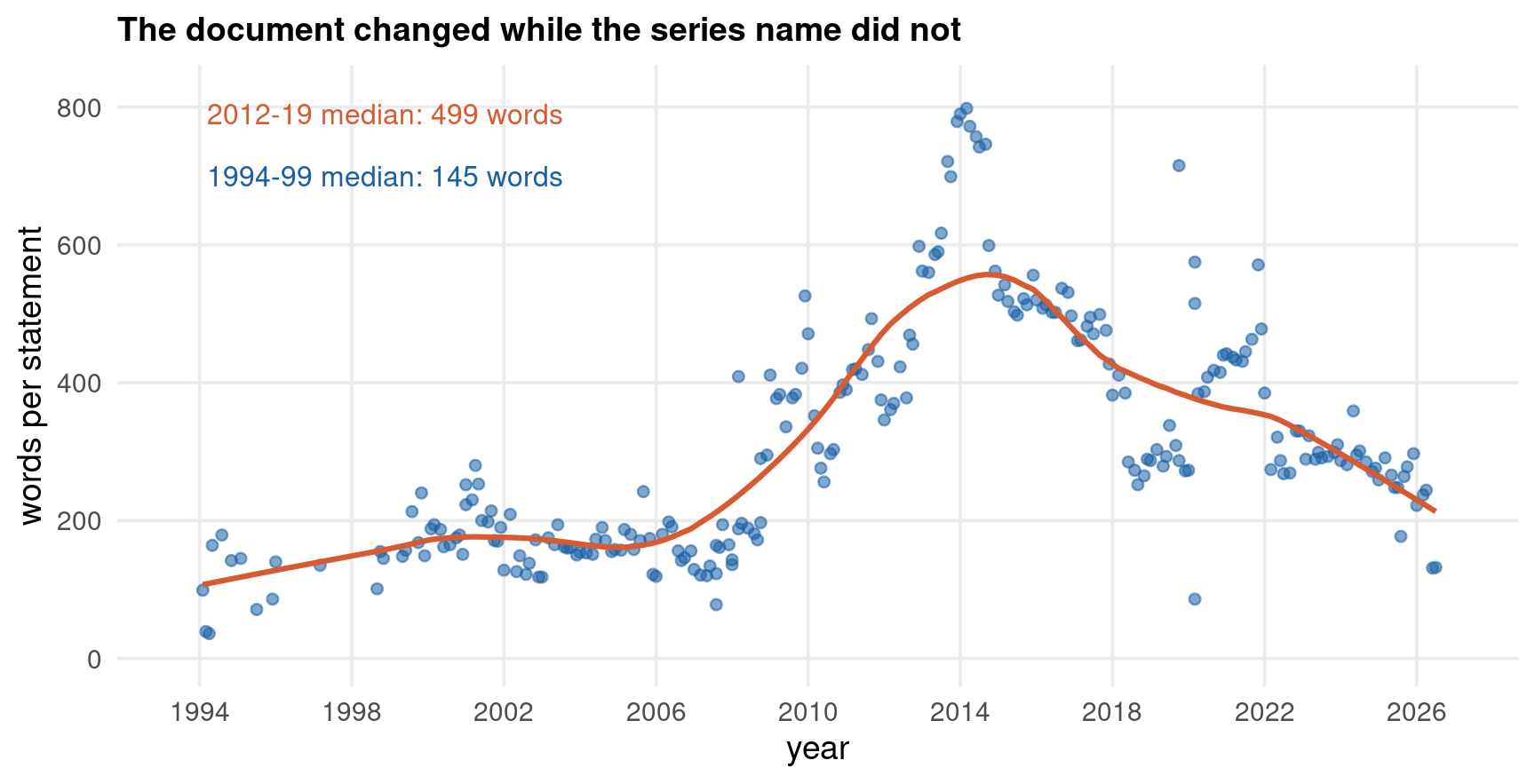
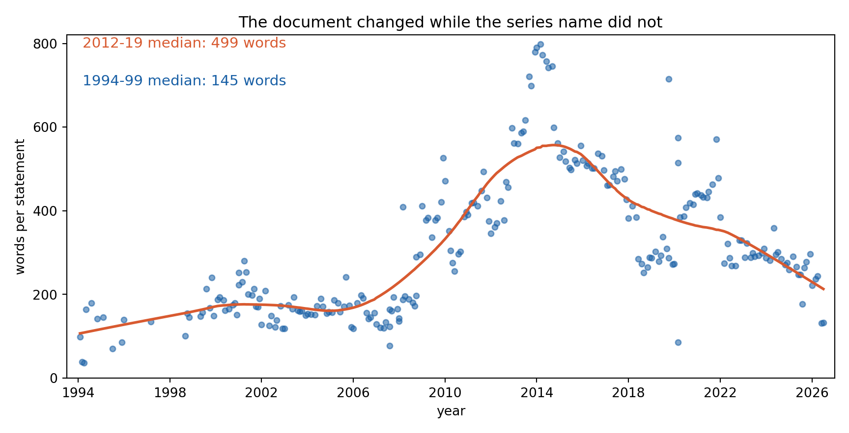
Code
b   = m.coef_[0]
sel = np.where(b != 0)[0]

pr = cross_val_predict(LogisticRegression(C=m.C_[0], penalty="l1",
                                          solver="liblinear", max_iter=5000),
                       X, y, cv=splits, method="predict")

out  = (f"n = {len(y)}, p = {p}\n"
        f"C = {m.C_[0]:.4g}  ->  lambda = {1 / (m.C_[0] * len(y)):.5f}\n"
        f"selected: {len(sel)} terms\n\ntop 12 selected terms by |coef|:\n")
for j in sel[np.argsort(-np.abs(b[sel]))][:12]:
    out += f"  {terms[j]:<12} {b[j]:9.2f}\n"
out += (f"\n10-fold CV accuracy {np.mean(pr == y):.3f}"
        f"   (always-hold baseline {1 - y.mean():.3f})\n")

import sys
nw = sys.stdout.write(out)
n = 245, p = 473
C = 17.01  ->  lambda = 0.00024
selected: 25 terms

top 12 selected terms by |coef|:
  rais             73.88
  interest         30.40
  imbal            30.27
  robust           26.36
  respond          25.72
  purchas         -22.88
  fulfil           22.66
  avail           -21.92
  order            20.44
  actual           18.96
  suppli           17.73
  possibl          17.60

10-fold CV accuracy 0.878   (always-hold baseline 0.796)
Code
sys.stdout.flush()
Code
* the vocabulary supplies both the idf weights and the variable names
quietly import delimited "../data/txt-vocab.csv", clear varnames(1)
forvalues j = 1/473 {
    local nm`j' = term[`j']
}
keep term_id df
tempfile voc
quietly save `voc'

quietly import delimited "../data/txt-labels.csv", clear varnames(1)
quietly gen long doc_id = _n
quietly gen byte y = next_action == "hike"
quietly replace y = . if !inlist(next_action, "hike", "hold", "cut")
keep doc_id y
tempfile lab
quietly save `lab'

* tf-idf while the matrix is still long, then reshape - far cheaper than
* looping over 473 columns
quietly import delimited "../data/txt-dtm.csv", clear varnames(1)
quietly bysort doc_id: egen double tot = total(count)
quietly merge m:1 term_id using `voc', nogenerate keepusing(df)
quietly gen double x = (count / tot) * ln(246 / df)
keep doc_id term_id x
quietly reshape wide x, i(doc_id) j(term_id)
foreach v of varlist x* {
    quietly replace `v' = 0 if missing(`v')
}
forvalues j = 1/473 {
    capture quietly rename x`j' t_`nm`j''
}
quietly merge 1:1 doc_id using `lab', nogenerate
quietly drop if missing(y)

quietly lasso logit y t_*, selection(cv) rseed(14159) nolog
display "n = " e(N) ", p = 473"
display "lambda (CV) = " %7.5f e(lambda_sel) "   selected: " e(k_nonzero_sel) " terms"
display _newline "selected terms, penalized coefficients:"
lassocoef, display(coef, penalized) sort(coef, penalized) nofvlabel
n = 245, p = 473

lambda (CV) = 0.04030   selected: 31 terms


selected terms, penalized coefficients:


------------------------
             |    active
-------------+----------
      t_rais |  74.94772
      t_caus |  73.76424
      t_take |  52.26545
   t_roughli |  35.18854
   t_respond |   33.3729
    t_expect |  26.66219
     t_imbal |  24.03262
   t_prevail |  23.41553
     t_order |  16.72365
  t_interest |  16.13057
     t_remov |  15.82517
     t_oblig |  15.42749
     t_trend |  15.27039
   t_describ |  12.59221
   t_contain |  11.16681
     t_stanc |  9.788334
      t_hous | -8.888779
   t_outlook | -8.273382
    t_advanc | -8.076494
    t_especi |   7.40726
   t_increas |  6.651271
      t_issu |  4.968961
       t_rel |  4.217872
    t_actual |  3.522342
  t_diminish | -3.303685
   t_possibl |  3.236465
     t_lower | -2.690888
       _cons | -2.665986
      t_tool |  -2.54008
      t_move |  2.283004
      t_time | -1.726188
t_strengthen |  .0071822
------------------------
Legend:
  b - base level
  e - empty cell
  o - omitted

Three Lassos, Three Answers

The three implementations do not select the same terms, and they do not select the same number of terms:

\(\lambda\) rule Terms selected
R glmnet lambda.1se 16
Python scikit-learn CV-minimising C 25
Stata lasso logit CV-minimising \(\lambda\) 31

None of that is a bug. Three things differ and cannot be made to agree:

  • the \(\lambda\) grid — each package builds its own, on its own scale (\(\lambda\), \(C = 1/n\lambda\), or Stata’s internal path)
  • the selection rule — R’s lambda.1se is deliberately more conservative than the CV minimum the other two use
  • the fold assignment — R and Python here share deterministic folds, but Stata’s lasso takes only a seed, not a fold map

Add the Part 2 result — correlated columns mean Lasso picks one member of a group arbitrarily — and the selected set is not an estimand. It is not stable across software, across seeds, or across bootstrap samples. Anything you say about which words matter rests on it, and it is the least reliable output the method has.

Intersecting the three selections leaves 10 terms chosen by every implementation:

\[ \{\, \texttt{rais},\; \texttt{imbal},\; \texttt{interest},\; \texttt{caus},\; \texttt{respond},\; \texttt{contain},\; \texttt{oblig},\; \texttt{order},\; \texttt{roughli},\; \texttt{trend} \,\} \]

And rais — the stem of raise — is the largest coefficient in all three, at \(77.7\) (R), \(73.9\) (Python) and \(74.9\) (Stata). When the packages agree, they agree strongly.

Now read the ten terms as an economist rather than as a modeller:

  • rais, interest, imbal — genuine policy language. “Raise the target range”; “imbalances” is the Committee’s own risk-assessment vocabulary of the 2000s
  • oblig, order, containboilerplate. They come from the pre-2000 formula “in order to fulfill its obligation”, which vanished when the statement was redesigned
  • caus, respond, roughli, trend — ambiguous, and roughli (“roughly balanced risks”) is another period-specific formula

So roughly half of the most stable, most replicable output of the method is not measuring policy stance at all. It is measuring when the document was written, and the pre-2000 era happens to be one where hikes were frequent.

The temptation is to read a selected word list as a description of what drives the outcome. It is not, for three separate reasons.

1. Selection is prediction, not interpretation. The Lasso’s objective is out-of-sample loss. A term earns its place by improving prediction, and a period marker predicts beautifully in a corpus with time-varying base rates — without being a cause of anything.

2. The omitted correlated terms are equally good. If inflat and price carry the same signal, the Lasso keeps one and discards the other. The discarded one is not “unimportant”; it is redundant, which is a different claim.

3. Post-selection inference is not the naive inference. The coefficients above were chosen and estimated on the same data, so their standard errors are not what a regression table would report:

\[ \text{the distribution of } \hat\beta_j \mid \{ j \text{ selected} \} \;\neq\; \text{the distribution of } \hat\beta_j \]

That is the Leeb–Pötscher problem, and the Machine Learning — Regularisation deck handles it. Here the point is narrower and prior to it: before asking whether the standard error is right, ask whether the word is a concept.

The practical test, which costs nothing: look at the selected words. If they include month names, place names, or the boilerplate of one era, your classifier has learned the calendar. That is a real finding about the corpus and a fatal one about the construct.

Multinomial Inverse Regression

Taddy (2013) makes a structural observation. The forward regression asks a hard question — the outcome on 473 correlated, sparse columns. The inverse regression asks an easy one: model the text as generated by the outcome.

\[ \underbrace{y_i \;\leftarrow\; \mathbf{c}_i}_{\text{forward: } p \gg n} \qquad\text{versus}\qquad \underbrace{\mathbf{c}_i \;\leftarrow\; y_i}_{\text{inverse: one regressor}} \]

Model the counts as multinomial with the outcome shifting the log-odds of each term:

\[ \mathbf{c}_i \;\sim\; \text{Multinomial}\bigl(m_i, \; \mathbf{q}_i \bigr), \qquad q_{ij} \;=\; \frac{\exp(\alpha_j + \varphi_j\, y_i)}{\sum_{l} \exp(\alpha_l + \varphi_l\, y_i)} \]

Each \(\varphi_j\) is estimated from a one-regressor problem, so the curse of dimensionality is gone. Then collapse the document back to a single number with the fitted loadings — Taddy’s sufficient reduction score:

\[ \hat z_i \;=\; \frac{\boldsymbol\varphi'\mathbf{c}_i}{m_i} \]

which is a sufficient statistic for \(y_i\) under the model. Note what it looks like: a dictionary whose weights were estimated rather than asserted. MNIR is the bridge between the two halves of this part.

Buys. A low-dimensional, interpretable score; estimation that parallelises across terms; and a natural place to put covariates — \(\varphi_j\) can load on several outcome variables at once, which is how Taddy handles controls.

Assumes, and these are strong:

  • the multinomial is correctly specified, so word counts within a document are independent given \(y_i\) — which bigrams in Part 2 already showed to be false
  • the sufficient reduction is sufficient, meaning \(y_i \perp \mathbf{c}_i \mid \hat z_i\); if the text carries information about \(y_i\) beyond the linear score, it is discarded by construction
  • the direction of the model is generative, so it is a statement about how documents are written, not about what a reader infers

The generated-regressor problem does not go away — it sharpens. \(\hat z_i\) is now explicitly \(\boldsymbol{\hat\varphi}'\mathbf{c}_i / m_i\), a function of estimated parameters, so Part 1’s variance correction \(\mathbf{G}\operatorname{Var}(\hat{\boldsymbol\theta})\mathbf{G}'\) is not optional bookkeeping: it is the whole difference between MNIR and a dictionary. Taddy’s own recommendation is to bootstrap the two stages jointly.

Dictionary versus Supervised

Dictionary Supervised (Lasso) MNIR
Weights asserted estimated estimated
Needs labels no yes yes
Overfits cannot yes, needs CV yes
Portable to a new corpus yes no — refit no — refit
Stable term list yes, by construction no more so than Lasso
Uses corpus-specific signal no yes yes
Generated-regressor problem mild — no \(\hat\theta\) severe severe, explicit
On this corpus, \(\kappa\) / CV accuracy 0.381 CV accuracy 0.849

The row that decides most applications is “needs labels”. A supervised method cannot exist without a label produced some other way, and producing one is the expensive part — which is exactly the promise Part 6 examines.

Use a dictionary when the construct is well defined in advance, the corpus spans regimes or languages you want a single scale across, transparency matters more than fit, or you have no labels. Then validate it anyway — the step Part 3 exists to insist on.

Use a supervised method when you have a credible label, the corpus is homogeneous, and prediction is the goal. Report the CV curve, look at the selected words for calendar artefacts, and do not interpret the coefficients as a topic.

Neither is a licence to skip Part 1. Both produce a \(\hat z_i\) that goes into a regression with an \(\varepsilon\) that already knows about it. The dictionary’s error is misspecification you can inspect; the supervised method’s is estimation error you must propagate. The second is bigger, and the one that gets reported less.

The remaining question is the one neither method answers: what if you never fixed the categories at all, and asked the corpus what it is about? That is Part 4 — where Stata drops out.

Part 4 — Topic Models

πῶς εἶπας; ἀλλ’ ἦ καὶ σοφὸς λέληθας ὤν;

what? have you been wise all along without our noticing?

Εὐριπίδης, Ἄλκηστις 58

Latent Semantic Analysis

The tab count changes here, and stays changed until Part 7. Parts 1–3 ran in all three languages. Parts 4, 5 and 6 are R and Python only — Stata has no LDA, no word2vec or GloVe, no embedding type and no interface to a language model. txttool and ngram stop at the bag of words, which is where this part begins. Where a method is missing from one of the two remaining languages — the structural topic model, later in this part — the tab says so rather than quietly disappearing.

Before any probability model there is a purely mechanical answer to what is this corpus about? — factorise the matrix and keep the largest pieces.

Take the truncated singular value decomposition of the centred tf-idf matrix:

\[ \mathbf{X} \;\approx\; \mathbf{U}_k \boldsymbol\Sigma_k \mathbf{V}_k', \qquad \mathbf{U}_k \in \mathbb{R}^{n \times k}, \quad \mathbf{V}_k \in \mathbb{R}^{p \times k} \]

Each column of \(\mathbf{V}_k\) is a weighted list of terms — a direction in vocabulary space. Each row of \(\mathbf{U}_k \boldsymbol\Sigma_k\) places a document on those directions. That is LSA, and it is nothing more than principal components on a document-term matrix.

It has one property no probabilistic topic model has: it is deterministic. No seed, no sampler, no initialisation, and the SVD is unique up to sign. The two tabs below therefore agree to the digit — the only slide in Parts 4 to 6 where that is true.

And one property that disqualifies it as a topic model: loadings can be negative. A component with \(-0.48\) on slightli is not a topic a document can have \(-48\%\) of. LSA gives directions, not compositions, so “how much of topic 3 is in this document?” has no answer.

The variance is not concentrated. On this corpus:

\[ \text{comp 1: } 13.6\%, \quad \text{comp 2: } 10.4\%, \quad \text{first 5: } 39.1\%, \quad \text{first 10: } 52.6\% \]

and it takes 57 components to reach 90%. For \(p = 473\) that is not a low-dimensional object.

The first component is worth reading closely. Its heaviest loadings are

\[ \texttt{slightli}\,(-0.48), \quad \texttt{degre}\,(-0.45), \quad \texttt{associ}\,(-0.41), \quad \texttt{short}\,(-0.40) \]

which is not a subject at all. It is the 1990s sentence “decided to increase slightly the degree of pressure on reserve positions … associated with a small increase in short-term money market interest rates”. The second component picks up bank, discount, approv, request, director — the discount-rate paragraph that disappeared after 2002.

The two leading dimensions of this corpus are eras, not subjects — exactly what the Lasso found in Part 3, by a completely different route. When two unrelated methods both put the calendar first, that is a fact about the corpus, and it is the most important thing to know before interpreting anything downstream.

Code
library(Matrix)

dtm <- read.csv("../data/txt-dtm.csv")
voc <- read.csv("../data/txt-vocab.csv")
n   <- 246

C <- sparseMatrix(i = dtm$doc_id, j = dtm$term_id, x = dtm$count,
                  dims = c(n, nrow(voc)))

# tf-idf, then centre: LSA is PCA on the document-term matrix
X  <- as.matrix((C / pmax(rowSums(C), 1)) %*% Diagonal(x = log(n / voc$df)))
sv <- svd(scale(X, center = TRUE, scale = FALSE))
ve <- sv$d^2 / sum(sv$d^2)

cat(sprintf("comp 1 %.3f | comp 2 %.3f | first 5 %.3f | first 10 %.3f\n",
            ve[1], ve[2], sum(ve[1:5]), sum(ve[1:10])))
cat(sprintf("components needed for 90%% of variance: %d of %d\n",
            which(cumsum(ve) >= 0.9)[1], nrow(voc)))

for (k in 1:2) {
  o <- order(-abs(sv$v[, k]))[1:8]
  cat(sprintf("\ncomponent %d: %s\n", k,
              paste(sprintf("%s(%+.2f)", voc$term[o], sv$v[o, k]), collapse = " ")))
}
comp 1 0.136 | comp 2 0.104 | first 5 0.391 | first 10 0.526
components needed for 90% of variance: 57 of 473

component 1: slightli(-0.48) degre(-0.45) associ(-0.41) short(-0.40) interest(-0.26) action(-0.20) increas(-0.14) bank(-0.12)

component 2: bank(-0.38) discount(-0.38) approv(-0.27) slightli(+0.18) request(-0.16) associ(+0.15) degre(+0.15) director(-0.15)
Code
import numpy as np
import pandas as pd

dtm = pd.read_csv("../data/txt-dtm.csv")
voc = pd.read_csv("../data/txt-vocab.csv")
n, p = 246, len(voc)

C = np.zeros((n, p))
C[dtm["doc_id"] - 1, dtm["term_id"] - 1] = dtm["count"]

# tf-idf, then centre: LSA is PCA on the document-term matrix
X = (C / np.maximum(C.sum(1, keepdims=True), 1)) * np.log(n / voc["df"].values)
U, S, Vt = np.linalg.svd(X - X.mean(0), full_matrices=False)
ve = S**2 / (S**2).sum()
terms = voc["term"].values

out  = (f"comp 1 {ve[0]:.3f} | comp 2 {ve[1]:.3f} | "
        f"first 5 {ve[:5].sum():.3f} | first 10 {ve[:10].sum():.3f}\n")
out += (f"components needed for 90% of variance: "
        f"{int(np.argmax(np.cumsum(ve) >= 0.9)) + 1} of {p}\n")
for k in range(2):
    o = np.argsort(-np.abs(Vt[k]))[:8]
    out += "\ncomponent %d: %s\n" % (
        k + 1, " ".join(f"{terms[j]}({Vt[k, j]:+.2f})" for j in o))

import sys
nw = sys.stdout.write(out)
comp 1 0.136 | comp 2 0.104 | first 5 0.391 | first 10 0.526
components needed for 90% of variance: 57 of 473

component 1: slightli(-0.48) degre(-0.45) associ(-0.41) short(-0.40) interest(-0.26) action(-0.20) increas(-0.14) bank(-0.12)

component 2: bank(-0.38) discount(-0.38) approv(-0.27) slightli(+0.18) request(-0.16) associ(+0.15) degre(+0.15) director(-0.15)
Code
sys.stdout.flush()

LDA — The Generative Story

LDA fixes LSA’s defect by making the factorisation probabilistic and non-negative. A topic is a distribution over words; a document is a distribution over topics. Both are compositions, so they sum to one and can be read as shares.

The generative story — the fiction LDA asserts about how each document was written:

  1. For each topic \(k = 1, \dots, K\), draw a word distribution \(\boldsymbol\beta_k \sim \text{Dirichlet}(\eta)\)
  2. For each document \(i\), draw a topic mixture \(\boldsymbol\theta_i \sim \text{Dirichlet}(\alpha)\)
  3. For each of the \(m_i\) word slots, draw a topic \(z_{i\ell} \sim \text{Multinomial}(\boldsymbol\theta_i)\), then a word \(w_{i\ell} \sim \text{Multinomial}(\boldsymbol\beta_{z_{i\ell}})\)

Nobody believes step 3. It says an author picks each word independently by first rolling a die for its topic — no grammar, no order, no memory. It is the bag-of-words assumption from Part 2, now stated as a likelihood.

The defence is the usual one: the model is wrong, and the question is whether \(\boldsymbol\theta_i\) is useful. That is an empirical question, and the next three slides are about how badly it is normally answered.

Collecting the story, the probability of the corpus integrates out both sets of latent variables:

\[ p(\mathbf{W} \mid \alpha, \eta) = \prod_{i=1}^{n} \int p(\boldsymbol\theta_i \mid \alpha) \left[ \prod_{\ell=1}^{m_i} \sum_{k=1}^{K} p(z_{i\ell} = k \mid \boldsymbol\theta_i)\, p(w_{i\ell} \mid \boldsymbol\beta_k) \right] \mathrm{d}\boldsymbol\theta_i \]

The sum inside the product is what makes this hard: it couples \(\boldsymbol\theta\) and \(\boldsymbol\beta\), and the integral has no closed form.

Read as a factorisation, LDA approximates the normalised count matrix by a product of two non-negative, row-stochastic matrices:

\[ \underbrace{\mathbf{C}/m}_{n \times p} \;\approx\; \underbrace{\boldsymbol\Theta}_{n \times K} \; \underbrace{\mathbf{B}}_{K \times p}, \qquad \theta_{ik} \ge 0,\; \textstyle\sum_k \theta_{ik} = 1, \qquad \beta_{kj} \ge 0,\; \textstyle\sum_j \beta_{kj} = 1 \]

Those constraints are the whole difference from LSA, and they buy interpretability: \(\theta_{ik}\) is the share of document \(i\) that is about topic \(k\), and \(\hat z_i = \theta_{ik}\) is precisely the generated regressor Part 1 warned about.

Estimating LDA — Two Answers

The intractable integral has two standard approximations, and this deck’s two languages happen to use different ones — which matters more than anyone advertises.

Collapsed Gibbs sampling (R, topicmodels with method = "Gibbs"). Integrate out \(\boldsymbol\theta\) and \(\boldsymbol\beta\) analytically, then sample each word’s topic assignment from its full conditional:

\[ \Pr(z_{i\ell} = k \mid \mathbf{z}_{-i\ell}, \mathbf{w}) \;\propto\; \frac{n_{k, w_{i\ell}}^{-i\ell} + \eta}{n_{k,\cdot}^{-i\ell} + p\eta} \;\cdot\; \bigl(n_{i,k}^{-i\ell} + \alpha\bigr) \]

Asymptotically exact, and slow.

Variational Bayes (Python, scikit-learn). Replace the posterior with the closest factorised distribution and maximise a lower bound on the evidence:

\[ q(\boldsymbol\theta, \mathbf{z}, \boldsymbol\beta) = q(\boldsymbol\theta)\, q(\mathbf{z})\, q(\boldsymbol\beta), \qquad \max_{q} \; \mathcal{L}(q) \;\le\; \log p(\mathbf{W}) \]

Fast, deterministic given a seed, and biased — the factorisation understates posterior variance by construction.

Neither algorithm is re-taught here. Bayesian Computation in Economics and Econometrics owns the Gibbs sampler and the variational bound, including why VB understates posterior spread. LDA is that machinery applied to a multinomial mixture.

Before the code: expect disagreement, and know its sources. None of this is a bug.

  • Label switching. Topic 3 in R and topic 3 in Python are unrelated. Only the partition is identified, never the numbering. Any comparison must match topics by content.
  • Initialisation and seed. Both are stochastic. Refit with another seed and topics merge, split and reorder — which is why a topic share is a fragile regressor.
  • The objective differs. Gibbs targets the exact posterior, VB a bound on it. Their held-out perplexities are computed differently and are not on the same scale — the next slide makes that vivid.

The comparison here is therefore qualitative and explicit: do the two implementations find recognisably the same kinds of topic? On this corpus they do — a balance-sheet topic, a 1990s discount-rate topic, a modern dual-mandate topic — and the code matches them by a stated rule (the topic with the largest weight on a chosen stem), never by eye.

Code — LDA on the FOMC Corpus

Code
library(topicmodels)
library(slam)
set.seed(14159)

C <- sparseMatrix(i = dtm$doc_id, j = dtm$term_id, x = dtm$count,
                  dims = c(n, nrow(voc)), dimnames = list(NULL, voc$term))
M <- as.simple_triplet_matrix(as.matrix(C))

# text2vec also exports LDA(), perplexity(), terms() and logLik(); it is attached
# for Part 5, so every topicmodels call here is namespaced explicitly
fit <- topicmodels::LDA(M, k = 6, method = "Gibbs",
           control = list(seed = 14159, iter = 2000, burnin = 500, verbose = 0))

tt <- topicmodels::terms(fit, 8)
for (k in 1:6) cat(sprintf("topic %d: %s\n", k, paste(tt[, k], collapse = ", ")))

# match topics by a STATED rule, never by eye: the topic loading most heavily
# on a chosen stem
beta <- exp(fit@beta)
colnames(beta) <- voc$term
cat(sprintf("\nbalance-sheet topic (max beta on 'mortgag') : %d\n",
            which.max(beta[, "mortgag"])))
cat(sprintf("discount-rate topic  (max beta on 'discount'): %d\n",
            which.max(beta[, "discount"])))
topic 1: econom, continu, like, stabil, level, remain, price, financi
topic 2: inflat, support, econom, condit, expect, time, polici, financi
topic 3: longer, secur, back, agenc, mortgag, run, polici, consist
topic 4: growth, action, sustain, point, risk, bank, target, price
topic 5: inflat, monetari, remain, risk, rang, polici, outlook, assess
topic 6: inflat, expect, fund, labor, condit, econom, measur, indic

balance-sheet topic (max beta on 'mortgag') : 3
discount-rate topic  (max beta on 'discount'): 4
Code
from sklearn.decomposition import LatentDirichletAllocation

lda = LatentDirichletAllocation(n_components=6, random_state=14159,
                                learning_method="batch", max_iter=200)
theta = lda.fit_transform(C)

out = ""
for k in range(6):
    o = np.argsort(-lda.components_[k])[:8]
    out += f"topic {k + 1}: {', '.join(terms[o])}\n"

# match topics by a STATED rule, never by eye: the topic loading most heavily
# on a chosen stem
beta = lda.components_ / lda.components_.sum(1, keepdims=True)
jm = int(np.where(terms == "mortgag")[0][0])
jd = int(np.where(terms == "discount")[0][0])
out += (f"\nbalance-sheet topic (max beta on 'mortgag') : {beta[:, jm].argmax() + 1}\n"
        f"discount-rate topic  (max beta on 'discount'): {beta[:, jd].argmax() + 1}\n")

import sys
nw = sys.stdout.write(out)
topic 1: inflat, secur, longer, polici, labor, agenc, run, econom
topic 2: inflat, econom, polici, rang, monetari, appropri, continu, goal
topic 3: econom, continu, inflat, secur, remain, level, price, market
topic 4: inflat, growth, econom, price, risk, polici, remain, sustain
topic 5: bank, action, discount, econom, growth, approv, avail, point
topic 6: inflat, expect, econom, fund, condit, labor, rang, remain

balance-sheet topic (max beta on 'mortgag') : 1
discount-rate topic  (max beta on 'discount'): 5
Code
sys.stdout.flush()

Choosing \(K\)

Held-out perplexity. Fit on a training set, score the documents held out. Lower is better:

\[ \text{perplexity}(\mathcal{D}_{\text{test}}) = \exp\!\left\{ - \frac{\sum_{i \in \mathcal{D}_{\text{test}}} \log p(\mathbf{w}_i)} {\sum_{i \in \mathcal{D}_{\text{test}}} m_i} \right\} \]

Topic coherence, in the UMass form. For the top \(T\) terms of a topic, reward pairs that co-occur in the same documents. Higher — less negative — is better:

\[ \mathcal{C}_k = \frac{2}{T(T-1)} \sum_{a=2}^{T} \sum_{b=1}^{a-1} \log \frac{D(w_a, w_b) + 1}{D(w_b)} \]

where \(D(w)\) counts documents containing \(w\), and \(D(w_a, w_b)\) documents containing both. Coherence is a proxy for would a human call this a topic?

Both criteria, on 186 training and 60 held-out documents:

\(K\) R perplexity (Gibbs) R coherence Python perplexity (VB)
2 230.6 −0.273 255.1
4 203.2 −0.438 253.7
6 194.7 −0.418 269.3
8 187.5 −0.407 288.1
10 181.1 −0.483 310.0
12 179.9 −0.444 323.5
16 175.3 −0.504 344.0

Three failures, visible at once.

  • R’s perplexity falls monotonically. It picks \(K = 16\), and would pick \(K = 100\) if offered. A criterion with no interior optimum is not a selection rule.
  • The two languages point in opposite directions. Python’s variational bound rises after \(K = 4\). Same data, same grid, opposite advice — because Gibbs and VB score held-out documents differently, and the two columns are not on the same scale.
  • Coherence picks \(K = 2\), the one value guaranteed to be useless, and is otherwise noisy rather than single-peaked.

\(K\) is chosen by the researcher, for reasons outside the data, and every downstream standard error is conditional on that choice while being reported as though it were not. The defensible procedure: state \(K\), state why, and show the result at neighbouring \(K\) — a specification curve, again.

Code
set.seed(14159)
test  <- sample(n, 60)
train <- setdiff(1:n, test)

B <- as.matrix(C) > 0        # document indicator, for coherence

res <- data.frame()
for (K in c(2, 4, 6, 8, 10, 12, 16)) {
  f  <- topicmodels::LDA(M[train, ], k = K, method = "Gibbs",
            control = list(seed = 14159, iter = 600, burnin = 200, verbose = 0))
  pp <- topicmodels::perplexity(f, M[test, ],
                   control = list(seed = 14159, iter = 200, burnin = 100))

  # UMass coherence, averaged over topics, on the top 10 terms
  tt <- topicmodels::terms(f, 10)
  co <- mean(sapply(1:K, function(k) {
    w <- tt[, k]; s <- 0; m <- 0
    for (a in 2:10) for (b in 1:(a - 1)) {
      s <- s + log((sum(B[, w[a]] & B[, w[b]]) + 1) / sum(B[, w[b]]))
      m <- m + 1
    }
    s / m
  }))
  res <- rbind(res, data.frame(K = K, perplexity = round(pp, 1),
                               coherence = round(co, 3)))
}
print(res, row.names = FALSE)
  K perplexity coherence
  2      230.6    -0.273
  4      203.2    -0.438
  6      194.7    -0.418
  8      187.5    -0.407
 10      181.1    -0.483
 12      179.9    -0.444
 16      175.3    -0.504

perplexity decreases monotonically: it never selects a K
Code
rng   = np.random.RandomState(14159)
test  = rng.choice(n, 60, replace=False)
train = np.setdiff1d(np.arange(n), test)

out = f"{'K':>3}{'held-out perplexity':>22}\n"
for K in [2, 4, 6, 8, 10, 12, 16]:
    m = LatentDirichletAllocation(n_components=K, random_state=14159,
                                  learning_method="batch", max_iter=100).fit(C[train])
    out += f"{K:>3}{m.perplexity(C[test]):>22.1f}\n"
out += "\nthe variational bound RISES after K = 4 - the opposite of the R tab\n"

import sys
nw = sys.stdout.write(out)
  K   held-out perplexity
  2                 255.1
  4                 253.7
  6                 269.3
  8                 288.1
 10                 310.0
 12                 323.5
 16                 344.0

the variational bound RISES after K = 4 - the opposite of the R tab
Code
sys.stdout.flush()

Reading Tea Leaves

Chang, Boyd-Graber, Gerrish, Wang & Blei (2009) asked whether statistical measures of topic quality track what humans actually see. They ran two tasks on human subjects:

  • Word intrusion — show the top 5 terms of a topic plus one drawn from a different topic. Can a human find the intruder?
  • Topic intrusion — show a document with 3 of its high-probability topics plus 1 low-probability topic. Can a human find the intruder?

The finding: held-out likelihood is negatively correlated with human interpretability. The models that score best statistically are the ones humans find least coherent.

So the criterion on the previous slide does not merely fail to select \(K\) — over the range where it discriminates at all, it points away from the thing the topics are being used for. Optimising perplexity is optimising against interpretation.

It costs an afternoon and is the only validation of a topic model that means anything. Take the \(K = 6\) Gibbs fit from two slides back.

the balance-sheet topiclonger, secur, back, agenc, mortgag … plus an intruder

An economist reading that identifies the balance sheet immediately, and would spot discount or labor as the odd one out. That topic is real.

the residual topiceconom, continu, like, stabil, level, remain

Nothing here is the intruder, because nothing here is the topic. These are the high-frequency leftovers that survived the stopword list, collected into a bin. Every LDA fit has one or two, and they are never labelled as such in a paper.

The reporting rule that follows. If \(\hat z_i = \theta_{ik}\) is going into a regression, print the top terms of topic \(k\) in the paper and say who checked them. A topic share used as a variable, with no evidence that the topic is a concept, is a number with no referent — and Part 1’s \(u_i\) is then unbounded.

Structural Topic Models

Plain LDA gives every document the same prior over topics, which is exactly wrong for economics: a 1996 statement and a 2014 statement are not draws from a common \(\text{Dirichlet}(\alpha)\). The structural topic model lets covariates shift the prior:

\[ \boldsymbol\theta_i \;\sim\; \text{LogisticNormal}\bigl(\mathbf{X}_i\boldsymbol\Gamma, \; \boldsymbol\Sigma\bigr) \]

so topic prevalence is a regression, with \(\boldsymbol\Gamma\) estimated jointly with the topics rather than in a second step. Content covariates can shift \(\boldsymbol\beta_k\) too — the same topic worded differently in different regimes.

Why economists want this, in one line: estimating prevalence jointly with the topics propagates topic uncertainty into \(\hat{\boldsymbol\Gamma}\), which is exactly the Part 1 correction that a two-step fit LDA, then regress \(\hat\theta\) on \(X\) throws away.

Language boundary, declared. stm is an R package with no scikit-learn equivalent — Python’s LatentDirichletAllocation has no covariate interface. The nearest Python route is tomotopy’s DMRModel, which is not installed here. This slide is therefore R only, and says so rather than leaving a tab quietly missing.

Code
library(stm)
set.seed(14159)

fomc <- read.csv("../data/txt-fomc.csv")

# stm wants each document as a 2 x (non-zero terms) integer matrix
docs <- lapply(1:n, function(i) {
  s <- dtm[dtm$doc_id == i, ]
  rbind(as.integer(s$term_id), as.integer(s$count))
})

fit_stm <- stm(documents = docs, vocab = voc$term, K = 6,
               prevalence = ~ s(year), data = fomc,
               seed = 14159, max.em.its = 60,
               init.type = "Spectral", verbose = FALSE)

lt <- labelTopics(fit_stm, n = 8)
for (k in 1:6)
  cat(sprintf("topic %d: %s\n", k, paste(lt$prob[k, ], collapse = ", ")))

cat(sprintf("\noverall topic proportions: %s\n",
            paste(sprintf("%.3f", colMeans(fit_stm$theta)), collapse = "  ")))

b <- exp(fit_stm$beta$logbeta[[1]])
colnames(b) <- voc$term
cat(sprintf("balance-sheet topic (max beta on 'mortgag'): %d\n",
            which.max(b[, "mortgag"])))
topic 1: market, financi, credit, secur, bank, continu, back, condit
topic 2: inflat, econom, continu, secur, longer, remain, price, consist
topic 3: inflat, econom, polici, rang, monetari, appropri, goal, employ
topic 4: inflat, expect, econom, labor, condit, fund, rang, remain
topic 5: econom, action, growth, discount, approv, point, basi, current
topic 6: inflat, growth, econom, price, polici, risk, remain, moder

overall topic proportions: 0.056  0.174  0.213  0.182  0.172  0.202
balance-sheet topic (max beta on 'mortgag'): 1

Topics Over Time

Both tabs plot the same object: the yearly mean share of the balance-sheet topic, identified in each language by the stated rule — the topic with the largest weight on the stem mortgag. The topic numbers differ between the two; the series is comparable because the matching rule is, not because the indices are.

What it supports. The share sits low through the 1990s and 2000s, rises after 2008, peaks around 0.50 in the QE3 years, and falls back after 2015. That is a real feature of the documents, and it lines up with the balance-sheet programmes without having been told about them.

What it does not support — the whole caution:

  • It is not a measure of the size of the balance sheet. It measures how much of the statement was about it, which is a communication choice.
  • It is not comparable across the Part 1 regime break: the documents themselves changed shape in 2008 and again in 2020.
  • The peak is conditional on \(K = 6\). At \(K = 12\) the topic splits and each piece is smaller. No confidence band on this plot reflects that.

This is the natural end of Part 4. A topic share is a generated regressor resting on a model choice (\(K\)), an algorithm choice (Gibbs or VB), a seed and a preprocessing pipeline — four layers of researcher decision, none of which appears in a standard error. Part 6 asks whether a language model can shortcut all four, and finds that it relocates the problem rather than removing it.

Code
theta <- topicmodels::posterior(fit)$topics
kQE   <- which.max(beta[, "mortgag"])

tp <- aggregate(share ~ year,
                data = data.frame(year = fomc$year, share = theta[, kQE]),
                FUN = mean)

ggplot(tp) +
  aes(x = year, y = share) +
  geom_line(colour = "#185FA5", linewidth = 1.1) +
  geom_point(colour = "#185FA5", size = 2) +
  coord_cartesian(xlim = c(1994, 2026), ylim = c(0, 0.6)) +
  scale_x_continuous(breaks = seq(1994, 2026, 4)) +
  scale_y_continuous(breaks = seq(0, 0.6, 0.1)) +
  labs(x = "year", y = "mean topic share",
       title = "Balance-sheet topic share, K = 6 (Gibbs)")

Code
import matplotlib.pyplot as plt

fomc = pd.read_csv("../data/txt-fomc.csv")
kQE  = int(beta[:, jm].argmax())

tp = (pd.DataFrame({"year": fomc["year"], "share": theta[:, kQE]})
        .groupby("year", as_index=False)["share"].mean())

fig, ax = plt.subplots(figsize=(9, 4.4))
ax.plot(tp["year"], tp["share"], "-o", color="#185FA5", linewidth=2.0, markersize=5)
axopts = ax.set(xlim=(1994, 2026), ylim=(0, 0.6),
                xticks=range(1994, 2027, 4),
                yticks=[0.0, 0.1, 0.2, 0.3, 0.4, 0.5, 0.6],
                xlabel="year", ylabel="mean topic share",
                title="Balance-sheet topic share, K = 6 (variational)")
plt.tight_layout()
plt.show()

Part 5 — Embeddings

Ἑλένῃ δʼ ὅμοιον σῶμʼ ἔχουσʼ οὐ τὰς φρένας
ἔχεις ὁμοίας, ἀλλὰ διαφόρους πολύ.

a body like Helen’s — but the mind you have is not alike, it is very different

Εὐριπίδης, Ἑλένη 160–161

The Distributional Hypothesis

“You shall know a word by the company it keeps.” Firth’s slogan is the entire foundation of embeddings, and it is a strong empirical claim: words that appear in similar contexts have similar meanings, so a word can be represented by a summary of its contexts.

That is a genuine break with Parts 2 to 4. There, a word was an index — column inflat was as unrelated to column price as it was to mortgag, because the one-hot representation makes every pair of distinct terms orthogonal:

\[ \langle \mathbf{e}_j, \mathbf{e}_{j'} \rangle = 0 \quad \text{for all } j \neq j' \]

An embedding replaces that index with a dense vector \(\mathbf{v}_j \in \mathbb{R}^{50}\) in which distance means something, so treasuri can sit near secur without anyone declaring that it should.

Note what this does not require: no labels, no topics, no \(K\). Embeddings are unsupervised and estimated from co-occurrence alone — which is why they are trained on billions of tokens and then reused, rather than fitted to your corpus.

Fix a symmetric window of \(\pm w\) tokens. The co-occurrence matrix counts how often term \(j\) appears within that window of term \(j'\):

\[ X_{jj'} \;=\; \sum_{\text{corpus}} \mathbb{1}\{\, j' \text{ within } \pm w \text{ of } j \,\} \]

Every embedding method is a low-rank factorisation of a transform of this matrix:

\[ f(X_{jj'}) \;\approx\; \langle \mathbf{v}_j, \tilde{\mathbf{v}}_{j'} \rangle \]

with \(\mathbf{v}_j \in \mathbb{R}^{D}\) and \(D \ll p\). The methods differ in the transform \(f\) and the loss, not in the idea.

Similarity is then cosine, because vector length tracks frequency rather than meaning:

\[ \text{sim}(j, j') \;=\; \frac{\langle \mathbf{v}_j, \mathbf{v}_{j'} \rangle}{\lVert \mathbf{v}_j \rVert \, \lVert \mathbf{v}_{j'} \rVert} \;\in\; [-1, 1] \]

The window is a modelling choice, exactly like the ones in Part 2. A window of 2 captures syntax — words that fill the same grammatical slot. A window of 10 captures topic — words that appear in the same discussion. Both are called “similarity” and they are different objects. This deck uses \(w = 5\), and would get different neighbours at \(w = 2\).

word2vec and GloVe

Mikolov et al. (2013) do not factorise anything explicitly. Skip-gram trains a classifier to predict context words from a centre word, and keeps the weights:

\[ \max \; \sum_{\ell} \sum_{-w \le r \le w,\; r \ne 0} \log \Pr\bigl(t_{\ell+r} \mid t_{\ell}\bigr), \qquad \Pr(o \mid c) = \frac{\exp\langle \tilde{\mathbf{v}}_o, \mathbf{v}_c \rangle} {\sum_{j=1}^{p} \exp\langle \tilde{\mathbf{v}}_j, \mathbf{v}_c \rangle} \]

The denominator sums over the whole vocabulary at every token, so in practice it is replaced by negative sampling: distinguish the true context word from \(k\) random draws.

\[ \log \sigma\bigl(\langle \tilde{\mathbf{v}}_o, \mathbf{v}_c \rangle\bigr) \;+\; \sum_{i=1}^{k} \mathbb{E}_{j \sim P_n} \log \sigma\bigl(-\langle \tilde{\mathbf{v}}_j, \mathbf{v}_c \rangle\bigr) \]

Levy & Goldberg later showed this is implicitly factorising a shifted pointwise mutual information matrix — so it is the same idea after all.

Pennington, Socher & Manning (2014) go at the co-occurrence matrix directly, with a weighted least-squares loss on log counts:

\[ \min \; \sum_{j, j' = 1}^{p} h(X_{jj'}) \Bigl( \langle \mathbf{v}_j, \tilde{\mathbf{v}}_{j'} \rangle + b_j + \tilde b_{j'} - \log X_{jj'} \Bigr)^2 \]

with the weighting function that stops frequent pairs dominating:

\[ h(x) = \begin{cases} (x / x_{\max})^{3/4} & x < x_{\max} \\ 1 & \text{otherwise} \end{cases} \]

Two practical differences that matter for a small corpus: GloVe sees each pair once, using aggregate counts, so it is fast and deterministic given a seed; skip-gram streams the corpus repeatedly and is stochastic.

The final vectors are usually \(\mathbf{v}_j + \tilde{\mathbf{v}}_j\).

What the two code tabs actually run, and why. Python trains skip-gram word2vec. R does not train GloVe: text2vec’s implementation initialises its weights in C++ from a generator that set.seed() does not control, so it returns different neighbours on every render — fatal for a deck whose prose quotes its own output. The R tab therefore builds the embedding the explicit way — positive pointwise mutual information on the co-occurrence matrix, then a rank-50 SVD — which is deterministic, is exactly the factorisation written two slides ago, and is what Levy & Goldberg proved skip-gram is doing implicitly. So the two tabs are the explicit and implicit versions of one idea, and comparing them is meaningful rather than arbitrary.

Code — Embeddings Trained on the Corpus

Code
library(text2vec)
library(SnowballC)

fomc <- read.csv("../data/txt-fomc.csv")
stop <- readLines("../data/txt-stopwords.txt")

tokenise <- function(txt) {
  w <- strsplit(gsub("[^a-z ]", " ", tolower(txt)), "[[:space:]]+")[[1]]
  w <- w[nchar(w) > 2]
  wordStem(w[!(w %in% stop)], language = "porter")
}
toks <- lapply(fomc$text, tokenise)

it  <- itoken(toks, progressbar = FALSE)
vb  <- prune_vocabulary(create_vocabulary(it), term_count_min = 10)
tcm <- as.matrix(create_tcm(it, vocab_vectorizer(vb), skip_grams_window = 5))

# symmetrise the co-occurrence counts
X <- tcm + t(tcm)
diag(X) <- diag(X) / 2

# positive pointwise mutual information, then a rank-50 SVD: the explicit
# version of the factorisation the slide before this one wrote down
tot <- sum(X)
P   <- log((X * tot) / outer(rowSums(X), colSums(X)))
P[!is.finite(P)] <- 0
P[P < 0] <- 0

sv <- svd(P, nu = 50, nv = 50)
W  <- sv$u %*% diag(sqrt(sv$d[1:50]))
rownames(W) <- rownames(P)

cosine <- function(a, b) sum(a * b) / sqrt(sum(a^2) * sum(b^2))
neighbours <- function(w, k = 6) {
  v <- apply(W, 1, cosine, b = W[w, ])
  v <- sort(v, decreasing = TRUE)[2:(k + 1)]
  paste(sprintf("%s(%.2f)", names(v), v), collapse = " ")
}

cat(sprintf("tokens %d | embedding vocabulary %d (count >= 10) | 50 dimensions\n\n",
            sum(lengths(toks)), nrow(W)))
for (w in c("inflat", "labor", "secur", "risk", "tighten"))
  cat(sprintf("%-8s -> %s\n", w, neighbours(w)))
tokens 40715 | embedding vocabulary 495 (count >= 10) | 50 dimensions
inflat   -> rel(0.70) expect(0.64) near(0.59) item(0.58) longer(0.58) run(0.56)
labor    -> indic(0.69) suggest(0.57) underutil(0.57) improv(0.56) inform(0.56) sinc(0.55)
secur    -> treasuri(0.87) agenc(0.84) mortgag(0.81) hold(0.80) debt(0.77) matur(0.76)
risk     -> downsid(0.81) side(0.72) see(0.68) upsid(0.63) dual(0.61) outlook(0.60)
tighten  -> lag(0.60) cumul(0.57) monetari(0.55) account(0.50) slightli(0.49) privat(0.47)
Code
import re
import pandas as pd
from gensim.models import Word2Vec
from gensim.parsing.porter import PorterStemmer

fomc = pd.read_csv("../data/txt-fomc.csv")
stop = set(open("../data/txt-stopwords.txt").read().split())
ps   = PorterStemmer()

def tokenise(txt):
    w = re.sub(r"[^a-z ]", " ", txt.lower()).split()
    return [ps.stem(x) for x in w if len(x) > 2 and x not in stop]

toks = [tokenise(t) for t in fomc["text"]]

# skip-gram (sg=1), window 5, same minimum count as the R tab
m = Word2Vec(toks, vector_size=50, window=5, min_count=10, sg=1,
             seed=14159, workers=1, epochs=200)

out = (f"tokens {sum(len(t) for t in toks)} | "
       f"embedding vocabulary {len(m.wv)} (count >= 10) | 50 dimensions\n\n")
for w in ["inflat", "labor", "secur", "risk", "tighten"]:
    nb = " ".join(f"{a}({b:.2f})" for a, b in m.wv.most_similar(w, topn=6))
    out += f"{w:<8} -> {nb}\n"

import sys
nw = sys.stdout.write(out)
tokens 40715 | embedding vocabulary 495 (count >= 10) | 50 dimensions

inflat   -> expect(0.81) remain(0.55) run(0.55) object(0.54) continu(0.51) energi(0.51)
labor    -> condit(0.72) indic(0.69) improv(0.64) financi(0.54) modestli(0.51) develop(0.49)
secur    -> treasuri(0.90) agenc(0.86) mortgag(0.80) hold(0.77) billion(0.75) back(0.72)
risk     -> outlook(0.75) downsid(0.60) econom(0.54) global(0.49) roughli(0.48) pose(0.48)
tighten  -> first(0.47) slightli(0.47) firm(0.44) degre(0.44) lag(0.42) fiscal(0.40)
Code
sys.stdout.flush()

What the Vectors Learned, and What They Did Not

Read the two tables side by side. Where a term is frequent and its contexts are consistent, the explicit and implicit factorisations agree despite being different algorithms:

Term R (PPMI + SVD) top neighbours Python (skip-gram) top neighbours
secur treasuri, agenc, mortgag, hold, debt treasuri, agenc, mortgag, hold, billion
labor indic, suggest, underutil, improv condit, indic, improv, financi
risk downsid, side, see, upsid outlook, downsid, econom, global
inflat rel, expect, near, longer, run expect, remain, run, object

Nobody told either model that Treasury securities, agency debt and mortgage-backed securities belong together. That grouping is the balance-sheet vocabulary, recovered from co-occurrence alone — the same object LDA found as a topic and the Lasso found as a cluster of correlated columns, arrived at a third way.

Now tighten, the term an economist would most want:

top neighbours
R (PPMI + SVD) lag (0.60), cumul (0.57), monetari (0.55), account (0.50)
Python (skip-gram) first (0.47), slightli (0.47), firm (0.44), degre (0.44)

The two share exactly one neighbour, lag, and Python’s similarities top out at \(0.47\) against \(0.80\)\(0.90\) for secur. R’s list is the more defensible — cumulative tightening acts with a lag is real policy language — but the point is that you could not have known which to trust without checking, and cosine similarity reports the noisy case as a number between 0 and 1 with no warning attached.

This corpus is far too small to train embeddings, and that is the point of showing it. 40,715 tokens; published word2vec vectors are trained on \(10^{9}\)\(10^{11}\). The rule of thumb is millions of tokens minimum, and no diagnostic in either package will tell you that you are below it. If you must have embeddings for a small corpus, use pre-trained vectors — and then inherit whatever corpus they were trained on, which is its own measurement problem.

The famous demonstration is that vector arithmetic encodes relations:

\[ \mathbf{v}_{\text{king}} - \mathbf{v}_{\text{man}} + \mathbf{v}_{\text{woman}} \;\approx\; \mathbf{v}_{\text{queen}} \]

Three things are usually omitted when this is shown.

  • The query word is excluded from the answer set by construction. king, man and woman are removed before the nearest neighbour is taken. Leave them in and the nearest vector to the arithmetic is usually king itself.
  • Accuracy on standard analogy benchmarks is far from perfect — strong on geography and morphology, weak on almost everything abstract. The published examples are the successes.
  • The relation is not a fixed offset. There is no single “gender vector”; the difference \(\mathbf{v}_a - \mathbf{v}_b\) varies substantially across pairs of the same relation.

For economics the consequence is direct: do not build a measure out of a vector offset — a “hawkishness direction” defined as \(\mathbf{v}_{\texttt{tighten}} - \mathbf{v}_{\texttt{eas}}\) inherits all three problems, plus, on this corpus, two vectors that the previous tab just showed to be noise.

From Words to Documents

An embedding gives a vector per word. A regression needs a number per document. Three standard bridges, in increasing order of ambition.

1. Mean pooling. Average the word vectors:

\[ \mathbf{d}_i \;=\; \frac{1}{m_i} \sum_{\ell = 1}^{m_i} \mathbf{v}_{t_{i\ell}} \]

Simple, and surprisingly hard to beat. It is also exactly a bag of words again — order is destroyed, and the average is dominated by frequent, uninformative terms.

2. SIF — smooth inverse frequency (Arora, Liang & Ma). Weight each word by how surprising it is, then remove the first principal component of the resulting document vectors:

\[ \mathbf{d}_i = \frac{1}{m_i} \sum_{\ell} \frac{a}{a + \Pr(t_{i\ell})} \, \mathbf{v}_{t_{i\ell}}, \qquad \mathbf{d}_i \leftarrow \mathbf{d}_i - \mathbf{u}\mathbf{u}'\mathbf{d}_i \]

The weighting is tf-idf’s logic in a different costume; the projection removes a common component that is mostly syntax. It beats mean pooling reliably and costs one extra line.

3. doc2vec. Train a vector per document jointly with the word vectors, by adding a document token to every context. Elegant, and it introduces a new problem: a document vector for a new document must itself be inferred by gradient descent, so \(\hat z_i\) for an out-of-sample document is a stochastic quantity that differs every time you compute it.

Every route from words to documents throws away word order, or introduces inference noise, or both. There is no lossless bridge — which is why the honest comparison for an economics application is usually mean-pooled embeddings versus tf-idf, and tf-idf wins more often than the literature suggests.

Everything above gives a word one vector. But securities in “purchases of agency securities” and in “securities markets were volatile” are not the same word, and a single vector must average the two senses.

Transformers (Vaswani et al., 2017; BERT, Devlin et al., 2019) drop that assumption. The representation of a token is a function of the whole sentence:

\[ \mathbf{v}_{t_\ell} \;=\; g\bigl(t_1, \dots, t_{m}\bigr)_\ell \]

so the same word gets a different vector in every context, and there is no vocabulary-indexed lookup table at all.

What this buys, and what it costs:

  • Polysemy is handled; negation and syntax survive; performance on almost every benchmark improves
  • No fixed vocabulary means no interpretable coordinates — you cannot ask “which term drives this dimension?”
  • The model was pre-trained on a corpus you did not choose, at a date you must record
  • A GPU, a download, and a version number that will move

No transformer is trained in this deck, deliberately: the render must stay offline, deterministic and CPU-only. The conceptual point is what carries into Part 6 — once the representation is a function of a pre-trained model, the model version is part of your measurement, and it must be reported like a data vintage.

Embeddings as Regressors

Put a document embedding into a regression and Part 1’s equation returns with every term inflated:

\[ y_i \;=\; \alpha \;+\; \boldsymbol\gamma' \hat{\mathbf{d}}_i \;+\; \mathbf{x}_i'\boldsymbol\beta \;+\; \varepsilon_i, \qquad \hat{\mathbf{d}}_i \in \mathbb{R}^{50} \]

Four things are worse than for a dictionary score or a topic share.

  • Dimension. \(\hat{\mathbf{d}}_i\) is 50 numbers, not one. With \(n = 246\) that is a fifth of the sample spent on a regressor with no units.
  • No interpretation. \(\gamma_7\) is the coefficient on dimension 7, and dimension 7 is not anything. You cannot report it, sign it, or defend it.
  • Rotation invariance. The embedding is identified only up to an orthogonal transformation: \(\mathbf{Q}\hat{\mathbf{d}}_i\) fits equally well for any orthogonal \(\mathbf{Q}\). Individual coefficients are therefore not identified at all — only \(\lVert \boldsymbol\gamma \rVert\) and predictions are.
  • Estimation noise. \(\hat{\mathbf{d}}_i\) came from a stochastic fit on the same corpus, so the Part 1 variance correction applies to all 50 columns at once.

The one defensible use: prediction and similarity, where none of the four matters. Embeddings are excellent for “which two documents are alike?” — Hoberg and Phillips build an entire industry classification that way — and poor as a source of interpretable coefficients.

Bolukbasi et al. (2016) showed that embeddings trained on ordinary corpora encode social stereotypes in their geometry — the same offset arithmetic that produces king − man + woman ≈ queen also produces occupational analogies split by gender.

For an economist the framing is not primarily ethical, it is econometric:

\[ \hat{\mathbf{d}}_i \;=\; \mathbf{d}_i \;+\; \underbrace{\mathbf{u}_i}_{\text{not mean zero, not independent of } \mathbf{x}_i} \]

The embedding absorbed regularities of the training corpus that have nothing to do with your construct. If those regularities correlate with a covariate — region, period, author, firm size — then \(\mathbf{u}_i\) is correlated with \(\mathbf{x}_i\), and Part 1’s worst case applies: measurement error correlated with the regressors, with no sign result available.

Concretely, on this corpus: the leading LSA dimensions were eras, and the embedding is trained on the same co-occurrences. Any embedding-based measure here partly encodes when a statement was written — so regressing an outcome with a time trend on a document embedding will find something, and it will not be what the label says.

Part 6 — LLMs as Measurement Instruments

σοφὸς πεφυκὼς οὐδὲν ἐξαυδᾷς σοφόν.

born clever, you utter nothing clever

Σοφοκλῆς, Φιλοκτήτης 1244

The Proposition

Still two languages. Stata has no interface to a language model, so Part 6 is R and Python — and in truth the labelling happened in neither. It happened offline, once, and both tabs read the cached result. That is the argument of this part, arriving before the first slide.

Every method so far needed either a word list you wrote or a label somebody produced. The promise of a language model is that it removes both: describe the construct in a sentence, hand over the documents, get codes back.

\[ \hat z_i \;=\; g\bigl(d_i; \; \text{prompt}, \; \text{model}, \; \text{version}\bigr) \]

The appeal is real and worth stating plainly.

  • Scale. 10,000 documents in an afternoon, at a cost that rounds to zero against a research assistant’s time
  • No pipeline. No tokenisation, no stopwords, no stemmer, no \(K\) — Part 2’s twelve thousand forking paths simply do not arise
  • Context. Negation, irony, conditionals and subordinate clauses all survive, which no bag of words does
  • The construct is stated in English, so a referee can read your measurement instrument and disagree with it

Compare that last point with a topic share, where the “instrument” is a 475-dimensional Dirichlet posterior nobody can inspect. It is a genuine advance in transparency about intent.

And a genuine regression in transparency about execution. You can read the prompt; you cannot read the model. The next four slides are about what that costs in econometric terms — and the answer is not “nothing”, it is a specific, estimable, correctable bias.

ANTHROPIC_API_KEY is set in this environment and returns HTTP 401. Nothing in txt-data.R, and nothing in a render, can reach a model. That constraint forced the right design.

The codes in txt-labels.csv were produced once, offline, by a language model reading all 246 statements, and cached. The render only ever reads them, so:

  • the deck is deterministic — the same numbers on every render, forever
  • the deck is offline — no network, no key, no rate limit, no bill
  • the deck is reproducible by a reader who has neither a key nor the same model

This is not a workaround, it is the recommendation. A paper whose numbers change when a vendor ships a new model checkpoint is not reproducible research. Cache the model’s output as data, version it, and ship it with the replication package — exactly as you would a proprietary dataset you cannot redistribute.

Zero-Shot Coding, and the Three Prompts

Zero-shot means no labelled examples: the task is described and the model answers. Few-shot supplies a handful of coded examples first. Both are prompting, not training — no parameter is updated, and the model has no memory of your corpus between documents.

Formally the model returns a distribution over the label set, and the code you store is its arg-max:

\[ \hat z_i \;=\; \arg\max_{c \,\in\, \{\text{hawkish}, \text{neutral}, \text{dovish}\}} \; \Pr\bigl(c \mid d_i, \text{prompt}\bigr) \]

Two things follow immediately, and both matter econometrically.

  • The label set is yours. The model will place every document somewhere in it, including documents for which no category is right.
  • The arg-max discards the model’s own uncertainty. A document coded hawkish at \(0.98\) and one coded hawkish at \(0.34\) enter the regression identically.

The same 246 statements, three instructions. The target throughout is the forward-looking stance, validated against what the Committee did at its next meeting.

A — llm_base (all 246): “Read the FOMC statement. Ignoring the rate decision it announces, code the Committee’s forward-looking policy stance as hawkish, neutral or dovish. Answer with one word.”

B — llm_terse (60): “Hawkish, neutral, or dovish?”

C — llm_rich (60): a full rubric — weigh the balance-of-risks language, the relative emphasis on inflation against employment, and any explicit guidance about future adjustments; code hawkish if the next move is signalled as more likely up than down.

B and C run on a stratified subsample of 60 (20 cuts, 20 holds, 20 hikes, set.seed(14159)), because the point they make does not need 246 and the labelling is done by hand.

Note what separates A from B: a single clause, “ignoring the rate decision it announces”. The next slide is about how much that clause is worth.

Prompt Sensitivity

On the 60-statement subsample:

Comparison Agreement
A (base) vs C (rich rubric) 59 / 60
A (base) vs B (terse) 39 / 60
B (terse) vs C (rich) 38 / 60
All three agree 38 / 60

An elaborate rubric changes almost nothing — the rich prompt reproduces the base prompt on 59 of 60 documents. Deleting one clause changes 21 of 60.

And the disagreement is not scattered. Cross it with what the Committee actually did at that meeting:

Realized action A and B agree A and B differ
cut 19 1
hike 17 3
hold 3 17

The terse prompt is not measuring stance — it is reading the headline. Given no instruction to look past the announced decision, it agrees with the careful prompt on 36 of 40 meetings where the Committee moved, and disagrees on 17 of 20 where it did nothing. With no action to anchor on, a one-line prompt has nothing to say, and says “neutral”.

That is the whole prompt-sensitivity problem in one table. The variation is systematic and correlated with the outcome — holds are exactly the observations where forward guidance carries the information — so the induced measurement error is not noise. It is the non-classical kind from Part 1.

  • Publish the prompt verbatim, in the paper, not in a footnote. It is the instrument. A prompt you paraphrase is a specification you did not report.
  • Run at least two prompts and report agreement. One prompt is one specification; the spread across prompts is the closest thing to a standard error the method offers.
  • Look at where they disagree. If disagreement concentrates on a subgroup — as it does here, on holds — the error is correlated with your regressors and no attenuation result applies.
  • Fix the decoding. Temperature, top-\(p\) and seed are part of the instrument. Ours is a single greedy pass; a sampled pass would not reproduce.

Validation Against the Realized Action

Prompt A’s 246 codes against what the Committee did at its next meeting:

cut hold hike
dovish 31 66 1
neutral 6 34 5
hawkish 3 55 44

\[ \text{accuracy} = 0.445, \qquad \kappa = 0.243 \]

against an always-hold baseline of \(0.633\). So — exactly as in Part 3, and more sharply — the model is far worse than a trivial rule on accuracy while carrying real information, and only \(\kappa\) shows it.

Read the corners rather than the total. Of 40 next-meeting cuts the model called 31 dovish and only 3 hawkish; of 51 hikes it called 44 hawkish and only 1 dovish. It is very good at direction and very bad at timing — the 66 dovish and 55 hawkish calls that landed on holds are the model saying “a move is coming” before it came.

That is a substantive finding about forward guidance, not a failure of the model: the FOMC signals direction long before it acts, so a stance measure and a next-meeting indicator are not the same object even when the stance is read perfectly.

Collapse to the question the next slides need — does the model say hawkish, and does the Committee hike next time?

\[ z_i = \mathbb{1}\{\text{model says hawkish}\}, \qquad y_i = \mathbb{1}\{\text{next meeting hikes}\} \]

sensitivity specificity accuracy \(\kappa\)
\(z\) against \(y\) 0.880 0.703 0.739 0.420

The two misclassification rates that everything else depends on:

\[ \alpha_0 \;=\; \Pr(z_i = 1 \mid y_i = 0) \;=\; \mathbf{0.2974}, \qquad \alpha_1 \;=\; \Pr(z_i = 0 \mid y_i = 1) \;=\; \mathbf{0.1200} \]

They are very unequal, and that asymmetry is the whole story of the next slide: the model over-calls hawkish (it is early), and rarely misses a hike.

The Econometrics of a Noisy Label

For a continuous regressor, classical measurement error attenuates. For a binary one it cannot even be classical, and the reason is mechanical: if \(z_i^* = 1\), the error \(z_i - z_i^*\) can only be \(0\) or \(-1\). The error is deterministically negatively correlated with the truth:

\[ \operatorname{Cov}(z_i - z_i^*, \; z_i^*) \;<\; 0 \qquad \text{whenever } \alpha_1 > 0 \]

So Part 1’s classical result does not apply — but an exact one does. With misclassification independent of \(y\) given \(z^*\) (Aigner, 1973), the regression of \(y\) on the mismeasured \(z\) has probability limit

\[ \operatorname{plim} \hat\gamma \;=\; \gamma \cdot \bigl(1 - \alpha_0 - \alpha_1\bigr) \]

The attenuation factor is not a variance ratio, it is one minus the sum of the two error rates. Three consequences worth memorising:

  • Attenuation depends only on \(\alpha_0 + \alpha_1\), so a model that is right 74% of the time is not 74% as good — the rates enter additively.
  • If \(\alpha_0 + \alpha_1 > 1\) the sign flips. That is not a pathology; it is a classifier worse than a coin.
  • The factor is estimable whenever you have a validation subsample, which is exactly what a few hundred hand-coded documents buy you.

\[ 1 - \alpha_0 - \alpha_1 \;=\; 1 - 0.2974 - 0.1200 \;=\; \mathbf{0.5826} \]

A regression using the model’s label recovers 58% of the true coefficient. Put the other way: the reported effect is 42% too small, and no amount of data fixes it — \(n \to \infty\) leaves the bias untouched.

A researcher who reported the raw coefficient with a robust standard error would be reporting a number 1.7 times too small, with a confidence interval that does not contain the truth, and every diagnostic in the output would look fine.

The correction, when \(\alpha_0\) and \(\alpha_1\) are known or estimated:

\[ \hat\gamma^{\text{corrected}} \;=\; \frac{\hat\gamma}{1 - \hat\alpha_0 - \hat\alpha_1} \]

with a standard error that must account for the estimation of \(\hat\alpha_0\) and \(\hat\alpha_1\) — Part 1’s \(\mathbf{G}\operatorname{Var}(\hat{\boldsymbol\theta})\mathbf{G}'\) term, now with a name and a formula. The code slide does the arithmetic; the bootstrap for the standard error is Exercise 5 of Part 7.

Code — The Measurement-Error Arithmetic

Code
lab <- read.csv("../data/txt-labels.csv")

# the model's codes were produced offline, once, and cached: the render
# only reads them, so these numbers are identical on every build
ok <- !is.na(lab$next_action)
y  <- as.integer(lab$next_action[ok] == "hike")   # did the NEXT meeting hike?
z  <- as.integer(lab$llm_base[ok]   == "hawkish") # what the model said

# the two misclassification rates
a0 <- mean(z[y == 0])        # false positive: says hawkish, no hike
a1 <- mean(1 - z[y == 1])    # false negative: stays quiet, hike happens

cat(sprintf("n = %d\n", length(y)))
cat(sprintf("alpha0 = P(z=1 | y=0) = %.4f\n", a0))
cat(sprintf("alpha1 = P(z=0 | y=1) = %.4f\n", a1))
cat(sprintf("sensitivity %.3f | specificity %.3f | accuracy %.3f\n",
            1 - a1, 1 - a0, mean(y == z)))

lambda <- 1 - a0 - a1
cat(sprintf("\nattenuation factor 1 - a0 - a1 = %.4f\n", lambda))

# the linear probability model makes the arithmetic visible
fit <- summary(lm(y ~ z))$coefficients
cat(sprintf("\nmeasured  coefficient : %.4f  (se %.4f)\n", fit[2, 1], fit[2, 2]))
cat(sprintf("corrected coefficient : %.4f\n", fit[2, 1] / lambda))
cat(sprintf("the measured effect is %.0f%% too small\n", 100 * (1 - lambda)))
n = 245
alpha0 = P(z=1 | y=0) = 0.2974
alpha1 = P(z=0 | y=1) = 0.1200
sensitivity 0.880 | specificity 0.703 | accuracy 0.739

attenuation factor 1 - a0 - a1 = 0.5826

measured  coefficient : 0.3894  (se 0.0461)
corrected coefficient : 0.6684
the measured effect is 42% too small
Code
import numpy as np
import pandas as pd
import statsmodels.api as sm

lab = pd.read_csv("../data/txt-labels.csv")

# the model's codes were produced offline, once, and cached: the render
# only reads them, so these numbers are identical on every build
ok = lab["next_action"].notna().values
y  = (lab["next_action"][ok] == "hike").astype(int).values
z  = (lab["llm_base"][ok]    == "hawkish").astype(int).values

# the two misclassification rates
a0 = z[y == 0].mean()          # false positive: says hawkish, no hike
a1 = (1 - z[y == 1]).mean()    # false negative: stays quiet, hike happens

lam = 1 - a0 - a1
fit = sm.OLS(y, sm.add_constant(z)).fit()

out  = (f"n = {len(y)}\n"
        f"alpha0 = P(z=1 | y=0) = {a0:.4f}\n"
        f"alpha1 = P(z=0 | y=1) = {a1:.4f}\n"
        f"sensitivity {1 - a1:.3f} | specificity {1 - a0:.3f} | "
        f"accuracy {(y == z).mean():.3f}\n")
out += f"\nattenuation factor 1 - a0 - a1 = {lam:.4f}\n"
out += (f"\nmeasured  coefficient : {fit.params[1]:.4f}  (se {fit.bse[1]:.4f})\n"
        f"corrected coefficient : {fit.params[1] / lam:.4f}\n"
        f"the measured effect is {100 * (1 - lam):.0f}% too small\n")

import sys
nw = sys.stdout.write(out)
n = 245
alpha0 = P(z=1 | y=0) = 0.2974
alpha1 = P(z=0 | y=1) = 0.1200
sensitivity 0.880 | specificity 0.703 | accuracy 0.739

attenuation factor 1 - a0 - a1 = 0.5826

measured  coefficient : 0.3894  (se 0.0461)
corrected coefficient : 0.6684
the measured effect is 42% too small
Code
sys.stdout.flush()

Reproducibility

A dictionary is a file. A Lasso is a seed and a \(\lambda\). A language model is a service, and every part of it is subject to change without notice:

  • The weights. Vendors ship new checkpoints under the same name; “the same model” in March and September may not be.
  • The decoding. Temperature, top-\(p\), and whether the call is greedy or sampled all change the arg-max.
  • The context window. A long document silently truncated is a different document, and no error is raised.
  • Availability. Models are deprecated. A replication three years from now may not be able to call yours at all.

None of these appears in a regression table, and none has an analogue in any method in Parts 2 to 5.

Which makes caching not a convenience but the only honest option. Treat the model’s output as primary data with a vintage. Generate it once, store it, version it, and ship it. If your replication package requires a live API call, your results have a shelf life you did not choose and cannot see.

The reporting standard that follows from this whole deck, in one list. All of it is cheap; none of it is common.

The instrument

  • The model and version string, and the date every call was made
  • The prompt, verbatim, and the decoding parameters (temperature, seed, greedy or sampled)
  • How the output was parsed into a category, and what you did with unparseable replies

The validation

  • The size and construction of the validation sample, and who or what produced the reference labels
  • Sensitivity, specificity and \(\kappa\) — not accuracy, which an imbalanced label makes meaningless
  • At least two prompts, with an agreement rate and a breakdown of where they disagree

The econometrics

  • \(\hat\alpha_0\) and \(\hat\alpha_1\), and the implied attenuation factor \(1 - \hat\alpha_0 - \hat\alpha_1\)
  • The corrected coefficient alongside the raw one
  • A standard error that propagates the estimation of \(\hat\alpha_0\) and \(\hat\alpha_1\)

On this corpus that means: \(\hat\alpha_0 = 0.2974\), \(\hat\alpha_1 = 0.1200\), attenuation \(0.5826\), measured coefficient \(0.3894\), corrected \(0.6684\). Six numbers. A paper that reports only the first of the last two has understated its own finding by 42% — and it is the reader who cannot tell.

Part 7 — Applications, Exercises, Reading

οὔ φησι χρῆναι τοὺς νέους ἀσκεῖν, ἐγὼ δέ φημι.

he says the young should not train; I say they should

Ἀριστοφάνης, Νεφέλαι 1059

Application I — Central Bank Communication

The oldest and best-developed text-as-data application in macroeconomics: turn central bank language into a scalar and put it in a policy rule, a VAR or an event study.

The construction is Part 3’s dictionary score, aggregated to the year:

\[ \text{tone}_i \;=\; 100 \times \frac{\#\{\text{hawkish}\} - \#\{\text{dovish}\}}{m_i}, \qquad \overline{\text{tone}}_{y} \;=\; \frac{1}{n_y} \sum_{i \in y} \text{tone}_i \]

On this corpus the index runs from \(+7.31\) in 1994 — the year of the fastest tightening cycle in the sample — to \(-7.94\) in 1996 and \(-4.70\) in 2001. Its correlation with the contemporaneous target rate is \(0.304\).

Read the 1996 value as a warning, not a finding. 1996 contains a single statement, the January easing. A yearly average over one document is that document, and the index’s most extreme value is its least reliable — the Part 1 composition problem arriving in the final number. Any use of this series must weight by \(n_y\) or start in 2000.

Its correlation with the following year’s change in the target rate is only \(0.138\): the index tracks the stance the Committee is in far better than the one it is moving to. That gap is the whole difficulty of the literature.

Code
library(SnowballC)

fomc <- read.csv("../data/txt-fomc.csv")
lab  <- read.csv("../data/txt-labels.csv")
dict <- read.csv("../data/txt-dict.csv")
stop <- readLines("../data/txt-stopwords.txt")

tokenise <- function(txt) {
  w <- strsplit(gsub("[^a-z ]", " ", tolower(txt)), "[[:space:]]+")[[1]]
  w <- w[nchar(w) > 2]
  wordStem(w[!(w %in% stop)], language = "porter")
}
toks <- lapply(fomc$text, tokenise)
st   <- function(v) unique(wordStem(v, language = "porter"))

H <- st(dict$word[dict$category == "hawkish"])
D <- st(dict$word[dict$category == "dovish"])

tone <- sapply(toks, function(w) 100 * (sum(w %in% H) - sum(w %in% D)) / length(w))

yr <- aggregate(tone ~ year, data = data.frame(year = fomc$year, tone = tone),
                FUN = mean)

ggplot(yr) +
  aes(x = year, y = tone) +
  geom_hline(yintercept = 0, colour = "grey55") +
  geom_line(colour = "#185FA5", linewidth = 1.1) +
  geom_point(colour = "#185FA5", size = 2) +
  coord_cartesian(xlim = c(1994, 2026), ylim = c(-9, 9)) +
  scale_x_continuous(breaks = seq(1994, 2026, 4)) +
  scale_y_continuous(breaks = seq(-8, 8, 4)) +
  labs(x = "year", y = "mean hawkish - dovish score",
       title = "FOMC tone index, yearly mean (positive = hawkish)")

Code
import re
import numpy as np
import pandas as pd
import matplotlib.pyplot as plt
from gensim.parsing.porter import PorterStemmer

fomc = pd.read_csv("../data/txt-fomc.csv")
dic  = pd.read_csv("../data/txt-dict.csv")
stop = set(open("../data/txt-stopwords.txt").read().split())
ps   = PorterStemmer()

def tokenise(txt):
    w = re.sub(r"[^a-z ]", " ", txt.lower()).split()
    return [ps.stem(x) for x in w if len(x) > 2 and x not in stop]

toks = [tokenise(t) for t in fomc["text"]]
H = set(ps.stem(w) for w in dic.loc[dic["category"] == "hawkish", "word"])
D = set(ps.stem(w) for w in dic.loc[dic["category"] == "dovish",  "word"])

tone = np.array([100 * (sum(x in H for x in w) - sum(x in D for x in w)) / len(w)
                 for w in toks])

yr = (pd.DataFrame({"year": fomc["year"], "tone": tone})
        .groupby("year", as_index=False)["tone"].mean())

fig, ax = plt.subplots(figsize=(9, 4.4))
ax.axhline(0, color="grey")
ax.plot(yr["year"], yr["tone"], "-o", color="#185FA5", linewidth=2.0, markersize=5)
axopts = ax.set(xlim=(1994, 2026), ylim=(-9, 9),
                xticks=range(1994, 2027, 4), yticks=range(-8, 9, 4),
                xlabel="year", ylabel="mean hawkish - dovish score",
                title="FOMC tone index, yearly mean (positive = hawkish)")
plt.tight_layout()
plt.show()

Code
quietly import delimited "../data/txt-fomc.csv", clear varnames(1) ///
    bindquote(strict) maxquotedrows(unlimited)
quietly gen long doc_id = _n
keep doc_id year text
quietly replace text = ustrregexra(lower(text), "[^a-z]", " ")
quietly gen int nw = wordcount(text)
quietly expand nw
bysort doc_id: gen int k = _n
quietly gen str32 word = word(text, k)
drop text nw
quietly drop if strlen(word) <= 2

preserve
    keep word
    quietly bysort word: keep if _n == 1
    quietly txttool word, stopwords("../data/txt-stopwords.txt") stem generate(term)
    tempfile stems
    quietly save `stems'
restore
quietly merge m:1 word using `stems', nogenerate
quietly drop if term == ""

preserve
    quietly import delimited "../data/txt-dict.csv", clear varnames(1)
    quietly gen byte hawk = category == "hawkish"
    quietly gen byte dove = category == "dovish"
    quietly keep if hawk | dove
    quietly txttool word, stem replace
    quietly rename word term
    quietly collapse (max) hawk dove, by(term)
    tempfile dd
    quietly save `dd'
restore
quietly merge m:1 term using `dd', nogenerate keep(master match)
quietly replace hawk = 0 if missing(hawk)
quietly replace dove = 0 if missing(dove)

quietly gen byte one = 1
quietly collapse (sum) hawk dove ntok = one (first) year, by(doc_id)
quietly gen double tone = 100 * (hawk - dove) / ntok
quietly collapse (mean) tone, by(year)

twoway (function y = 0, range(1994 2026) lcolor(gs8))                        ///
       (line tone year, sort lcolor("24 95 165") lwidth(medthick))           ///
       (scatter tone year, mcolor("24 95 165") msize(small)),                ///
    legend(off)                                                              ///
    xscale(range(1994 2026)) xlabel(1994(4)2026)                             ///
    yscale(range(-9 9)) ylabel(-8(4)8)                                       ///
    xtitle("year") ytitle("mean hawkish - dovish score")                     ///
    title("FOMC tone index, yearly mean (positive = hawkish)", size(medium)) ///
    graphregion(color(white)) plotregion(color(white)) xsize(9) ysize(4.4)

graph export "../plots/txt-p7-index.png", replace width(1600)

Applications II and III

Firms file a legally mandated annual report with an explicit risk section (Item 1A). That makes it the closest thing text-as-data has to a panel: the same units, the same document type, every year, with an outcome attached.

  • Loughran & McDonald (2011) built the finance dictionary on exactly this corpus, and showed the General Inquirer misclassifies three-quarters of its negative hits.
  • Hoberg & Phillips (2016) compute pairwise similarity between 10-K product descriptions and derive an entire industry classification — text as a distance, not a score, which sidesteps most of Part 1’s problems.
  • Campbell et al. and a large literature since read Item 1A as a measure of firm-level risk and relate it to returns, volatility and financing.

Why it works better than the FOMC corpus. \(n\) is in the thousands, there is cross-sectional variation, and the disclosure requirement makes the corpus non-selected. Why it is still hard: the text is written by lawyers to minimise liability, boilerplate is copied year to year, and length responds to regulation rather than to risk.

Baker, Bloom & Davis (2016) built the Economic Policy Uncertainty index by counting newspaper articles containing terms from three sets simultaneously — economy, policy, and uncertainty — normalising by total articles, and standardising.

It is the canonical demonstration that a dictionary count can become an accepted macroeconomic time series. It is also the canonical demonstration of the risks:

  • the newspaper sample changes as titles are founded, merge and digitise — Part 1’s composition problem over 30 years
  • the term lists were audited by human readers on a sample of articles, which is why the index is trusted, and which almost nobody replicating the method bothers to do
  • the index is used as a shock in VARs, so all of Part 1’s generated-regressor concerns apply to structural impulse responses

Shapiro, Sudhof & Wilson (2022) do the same for news sentiment and — the part worth copying — publish their validation against human labels alongside the series.

Pitfalls

Each of these appeared somewhere in this deck, with a number attached.

  • Corpus selection. The FOMC issued a statement only when policy changed until 2000: 85% of the first 20 documents accompany a rate move, against 19% in 2012–2019. A series spanning both regimes compares different objects. (Part 1)
  • Preprocessing sensitivity. Four defensible pipelines moved the coefficient from \(0.886\) to \(1.159\) — about 1.4 standard errors — while leaving the sign and significance untouched. Magnitudes are not robust; signs often are. (Part 2)
  • Reifying the artefact. The leading LSA component, and half the Lasso’s stable core, are erasoblig, order, contain come from a pre-2000 formula. Two unrelated methods put the calendar first. (Parts 3, 4)
  • Accuracy on an imbalanced label. “Always predict hold” scores \(0.630\); the policy dictionary scores \(0.626\) and is genuinely informative (\(\kappa = 0.381\)). Reporting accuracy alone would have discarded a working measure. (Part 3)
  • \(\hat z\) used as if measured. A topic share rests on \(K\), an algorithm, a seed and a pipeline. None of those appears in its standard error. (Parts 1, 4)

Everything here is cheap, and its absence is what makes a text-as-data result impossible to evaluate.

The corpus

  • Source, access date, and why these documents and not others
  • \(n\), tokens, and the distribution of document length by period
  • What was removed and why — boilerplate, roll-calls, page furniture

The representation

  • Tokenisation rule, stopword list (as a file), stemmer and its implementation
  • Vocabulary size before and after the trim, and the trim rule
  • Weighting, and whether results survive counts versus tf-idf

The method

  • \(K\), \(\lambda\), dimension — and the result at neighbouring values
  • Seed, software versions, and whether the fit is deterministic
  • For topics: the top terms of any topic used as a variable

The validation — the section usually missing entirely

  • What the measure was validated against, and who produced that label
  • Agreement beyond chance (\(\kappa\)), not accuracy alone
  • How first-stage uncertainty enters the second-stage standard errors

Choosing a Method

Start from the estimand, never from the method.

If you need … Use Because Watch
A transparent index, comparable across corpora and decades Dictionary no estimation, so nothing to overfit and nothing to refit domain fit; validate it
The best prediction of a label you already have Supervised (Lasso) learns the weights instead of asserting them unstable selection; era artefacts
A description of what a corpus is about Topic model compositions are readable as shares \(K\) is yours; topics may be eras
Similarity between documents Embeddings distance is what they are good at needs millions of tokens
Coefficients you will interpret Not embeddings rotation invariance means individual coefficients are unidentified
A construct too subtle for a word list, with few labels LLM zero-shot coding needs no training set prompt sensitivity; version drift

The default that is usually right and rarely chosen: a small, hand-built, domain-specific dictionary, validated against a few hundred labels, reported with \(\kappa\). On this corpus 35 hand-picked stems beat a 1,197-stem general finance dictionary by more than a factor of two on \(\kappa\), and beat nothing else by being interpretable.

  • Machine Learning — Regularisation in Econometrics — the Lasso, cross-validation, post-selection inference and Leeb–Pötscher. Part 3 used them; it did not derive them.
  • Networks and Trade Analysis — the Clauset–Shalizi–Newman power-law test that Part 2 applied to word frequencies.
  • Bayesian Computation in Economics and Econometrics — the Gibbs sampler and the variational bound that estimate LDA in Part 4.
  • Causal Machine Learning in Econometrics — where a noisy generated regressor meets a causal estimand, and what DML does about it.

Exercises — Representation and Measurement

  1. Rebuild the corpus with a different tokeniser. Keep numbers as tokens ([^a-z0-9 ] instead of [^a-z ]). Report the new vocabulary size and the ten most frequent new terms. Does any rate level survive the \(df \ge 10\) trim, and what would that let you ask that the deck’s corpus cannot?
  2. Move the vocabulary trim. Rebuild the document-term matrix at \(df \ge 3\), \(\ge 10\) and \(\ge 25\). Tabulate vocabulary size, density, and the mean policy tone. Which of the three quantities is most sensitive, and why is that the opposite of what you would guess?
  3. Break the three-language parity deliberately. Run the R pipeline with wordStem(..., language = "english") (Snowball’s Porter2) instead of "porter". How many of the 1,720 word types change stem? Does the trimmed vocabulary size change?
  4. Test Zipf’s law on a subsample. Apply the CSN procedure to the 1994–2007 statements alone and to 2008–2026 alone. Compare \(\hat\alpha\), \(x_{\min}\) and \(n_{\text{tail}}\). What does the change in \(n_{\text{tail}}\) do to the power of the test?
  5. Bigrams before stopwords. Form bigrams on the raw token stream before removing stopwords, then remove any bigram containing a stopword. How many of the deck’s top-8 bigrams survive, and what happens to labor_condit and rang_fund?
  6. Document length as a confounder. Regress the policy tone score on n_words and a linear year trend. How much of the tone series is explained by how long the statement is?

Exercises — Modelling and Validation

  1. Build your own dictionary. Add ten hawkish and ten dovish stems of your own choosing before looking at the labels. Report accuracy and \(\kappa\) at \(\tau = 2\) against the realized action. Did you beat \(0.381\)? Now report how many versions you tried.
  2. The threshold is a researcher choice. Plot accuracy and \(\kappa\) for the policy dictionary over \(\tau \in [0, 4]\). At which \(\tau\) does \(\kappa\) peak, and how much higher is it than at the deck’s \(\tau = 2\)?
  3. Lasso stability. Refit the Part 3 Lasso with ten different fold assignments. How many terms appear in all ten selections, and how does that compare with the ten-term three-language stable core?
  4. Choose \(K\) honestly. Refit LDA at \(K \in \{4, 6, 8\}\) and rebuild the balance-sheet topic share each time, matching the topic by the stated mortgag rule. Plot the three series together. Is the 2014 peak robust in level, in timing, or in neither?
  5. Propagate the first-stage uncertainty. Bootstrap the corpus (resample documents with replacement), rebuild the policy tone index on each replicate, and re-run the logit predicting the next hike. Compare the bootstrap standard error with the one the logit reports. By what factor is the naive standard error too small?
  6. Reproduce the era artefact. Regress a “post-2000” dummy on the Lasso’s ten stable-core terms. How much of the era can those ten words explain, and what does that imply about interpreting them as policy language?
  7. A measure with no labels. You have 5,000 press releases and no coder. Write down, in half a page, the validation strategy you would use before putting your measure in a regression — and what you would report if it failed.

Further Reading

  • Chang et al. (2009), “Reading Tea Leaves”, NeurIPS — held-out likelihood is negatively correlated with interpretability. proceedings.neurips.cc
  • Loughran & McDonald (2011), J. Finance — what happens when a dictionary is applied outside its domain. doi:10.1111/j.1540-6261.2010.01625.x
  • Kelly, Manela & Moreira (2021), “Text Selection”, JBES — selection into the corpus as a modelling problem. doi:10.1080/07350015.2021.1947843
  • Gilardi, Alizadeh & Kubli (2023), PNAS — LLMs against crowd workers on annotation. doi:10.1073/pnas.2305016120
  • Ludwig, Mullainathan & Rambachan (2025), NBER wp 33344 — an econometric framework for an LLM as a measurement device. doi:10.3386/w33344

Thank You

Athanassios Stavrakoudis
Applied Informatics and Computational Economics Lab
Department of Economics
University of Ioannina, Greece

astavrak@uoi.gr · linkedin.com/in/astavrakoudis