# Unit roots and cointegration
library(tseries)    # adf.test, pp.test, kpss.test
library(urca)       # ur.df, ur.pp, ur.kpss, ur.ers, ur.za, ca.jo, cajorls
library(vars)       # VARselect, vec2var, irf, fevd, SVAR
library(tsDyn)      # VECM, TVECM, TVECM.HStest
library(dynlm)      # ECM via dynlm

# Long-run modelling and panels
library(ARDL)       # auto_ardl, bounds_f_test, bounds_t_test, multipliers
library(plm)        # pdata.frame, purtest, pmg

# Already loaded by the course setup:
# tidyverse, patchwork, sandwich, lmtest, modelsummaryUnit Roots, Cointegration and Vector Error Correction Models
Integration, Testing Strategies, Long-Run Equilibrium and Error Correction
using , &
30 July 2026
From Unit Roots to Error Correction
ἴσμεν γὰρ οὐδὲν τρανές, ἀλλʼ ἀλώμεθα·
we know nothing for certain — we wander
Σοφοκλῆς, Αἴας 23
Required Packages
import numpy as np
import pandas as pd
import matplotlib.pyplot as plt
import statsmodels.api as sm
from statsmodels.tsa.stattools import adfuller, kpss, coint
from statsmodels.tsa.vector_ar.vecm import (VECM, coint_johansen,
                                            select_coint_rank)
from statsmodels.tsa.ardl import ardl_select_order, ARDL, UECM
from arch.unitroot import ADF, PhillipsPerron, KPSS, DFGLS, ZivotAndrews
* Built in: dfuller, pperron, varsoc, vecrank, vec, irf, xtunitroot, xtset
* SSC packages, install once
ssc install dfgls, replace // DF-GLS (Elliott-Rothenberg-Stock)
ssc install zandrews, replace // Zivot-Andrews break test
ssc install kpss, replace // KPSS stationarity test
ssc install egranger, replace // Engle-Granger with MacKinnon values
ssc install ardl, replace // ARDL bounds test
ssc install xtwest, replace // Westerlund panel cointegration
ssc install xtpmg, replace // Mean Group / Pooled Mean GroupLiterature Review
| Paper | Contribution |
|---|---|
| Yule (1926) | Nonsense correlations between time series |
| Granger & Newbold (1974) | Spurious regression: high \(R^2\) with independent random walks |
| Dickey & Fuller (1979) | The ADF test for unit roots |
| Nelson & Plosser (1982) | Most macroeconomic series are I(1), not trend-stationary |
| Phillips (1986) | Asymptotic theory of regression with unit roots |
| Engle & Granger (1987) | Cointegration and the error correction representation |
| Phillips & Perron (1988) | Non-parametric correction for serial correlation |
| Johansen (1988) | Maximum likelihood cointegration rank tests |
| Johansen & Juselius (1990) | ML estimation and inference on cointegration |
| Johansen (1991) | Estimation and hypothesis testing of cointegrating vectors |
| Kwiatkowski et al. (1992) | KPSS: stationarity as the null hypothesis |
| Zivot & Andrews (1992) | Unit root with an endogenous structural break |
| Stock & Watson (1993) | DOLS: efficient estimation of cointegrating vectors |
| Elliott, Rothenberg & Stock (1996) | DF-GLS: GLS detrending improves power |
| Gregory & Hansen (1996) | Cointegration with an unknown regime shift |
| Balke & Fomby (1997) | Threshold cointegration |
| Pesaran, Shin & Smith (2001) | ARDL bounds test with mixed I(0)/I(1) regressors |
| Ng & Perron (2001) | Modified M-tests with GLS detrending |
| Enders & Siklos (2001) | Cointegration with threshold adjustment |
| Westerlund (2007) | Error-correction based panel cointegration tests |
| Shin, Yu & Greenwood-Nimmo (2014) | NARDL: asymmetric cointegration and dynamic multipliers |
The Method Family at a Glance
| Model | Key idea | Best use case |
|---|---|---|
| Unit root tests | Is the series \(I(0)\) or \(I(1)\)? | Always the first step |
| Engle-Granger | Residual test on a static regression | Bivariate, quick check |
| Johansen | Reduced-rank ML on the full system | \(K \ge 3\), multiple long-run relations |
| ARDL bounds | \(F\)-test on lagged levels | Mixed I(0)/I(1) regressors |
| Gregory-Hansen | Cointegration with a regime shift | Suspected structural break |
| ECM / VECM | Long-run equilibrium plus short-run dynamics | Standard cointegrated systems |
| SVECM | Permanent versus transitory decomposition | Structural interpretation |
| TVECM | Regime-specific adjustment speed | Transaction costs, arbitrage bands |
| NARDL | Asymmetric long-run effects | Sign-dependent pass-through |
| Panel CI | Pooled or heterogeneous error correction | Macro and finance panels |
Every tab in this deck reads the same CSV, so R, Python and Stata results are directly comparable.
| File | Contents | Source |
|---|---|---|
ur-vecm-sim.csv |
\(I(0)\), \(I(1)\), \(I(1)\)+drift, \(I(2)\), a cointegrated pair with \(\beta = 2\), and two independent walks | Simulated, seed 14159 |
ur-vecm-finland.csv |
lrm1, lny, lnmr, difp — 106 quarterly obs, 1958Q2–1984Q3 |
Johansen (1988) Finnish money demand |
ur-vecm-fred.csv |
lgdp, lpce, gs10, gs1 — 293 quarterly obs |
FRED |
ur-vecm-intqrt.csv |
r3, r6 — 124 quarterly obs |
Wooldridge, US T-bill rates |
ur-vecm-panel.csv |
48 US states × 17 years | Munnell (1990) |
ur-vecm-pwt.csv |
G7 log real GDP per capita | Penn World Table 10 |
The simulated file is the known-truth laboratory: every test can be scored against an answer we already have. The four real datasets are where the answer is unknown.
\[ \text{Plot} \;\rightarrow\; \text{Unit root tests} \;\rightarrow\; \text{Cointegration tests} \;\rightarrow\; \text{ECM / VECM} \;\rightarrow\; \text{IRF, FEVD, structure} \]
Each step conditions the next. The integration order decides whether cointegration testing is even meaningful; the cointegrating rank decides the shape of the VECM; the VECM is what makes the impulse responses interpretable.
Companion decks
Vector Autoregressive Methods and Local Projections develops the stationary VAR that sits underneath the VECM.
Bayesian Computation in Econometrics covers the Bayesian VAR alternative to the rank tests used here.
Part I — Integration and Spurious Regression
βαθύς γέ τοι Διρκαῖος ἀναχωρεῖν πόρος.
deep, to be sure, is the Dircean crossing to fall back through
Εὐριπίδης, Φοίνισσαι 730
The Spurious Regression Problem
Granger & Newbold (1974), following Yule (1926): regressing two independent random walks on each other produces
- an artificially high \(R^2\), often above 0.8
- a \(t\)-statistic on \(\hat\beta\) that appears overwhelmingly significant
- a Durbin-Watson statistic close to zero
The diagnostic that costs nothing: if \(R^2 > DW\) in a levels regression of \(I(1)\) variables, suspect a spurious regression.
Write the regression as
\[ y_t = \alpha + \beta x_t + u_t \]
Standard inference needs \(u_t \sim I(0)\). When \(y_t\) and \(x_t\) are both \(I(1)\) and not cointegrated, \(u_t\) is itself \(I(1)\) — it never returns to its mean, so the usual variance formulas do not apply.
OLS minimises \(\sum \hat u_t^2\) regardless. In any finite sample two independent random walks will share an apparent trend by chance, and OLS finds the linear combination that best exploits it.
\[ t_{\hat\beta} \;\xrightarrow{d}\; \text{a non-degenerate random variable, not } N(0,1) \]
The \(t\)-statistic diverges with \(T\) rather than settling down. More data makes the illusion stronger, not weaker.
Warning
If you regress \(I(1)\) variables without testing for cointegration, the results may be meaningless even with a \(p\)-value of 0.001. The whole of Parts I–III exists to keep you out of this trap.
The two escape routes:
- the variables are not cointegrated — model in first differences, accepting the loss of long-run information
- the variables are cointegrated — the levels regression is meaningful after all, and the error correction model of Part V is the right specification
Which one applies is an empirical question, and it is answered by the tests that follow.
Spurious Regression — Code
Code
sim_df <- read.csv("../data/ur-vecm-sim.csv")

fit <- lm(y_spur ~ x_spur, data = sim_df)
r2  <- summary(fit)$r.squared
dw  <- as.numeric(lmtest::dwtest(fit)$statistic)
cat(sprintf("R2 = %.3f   DW = %.3f   R2 > DW: %s\n", r2, dw, r2 > dw))
print(summary(fit)$coefficients)

sim_df |>
  select(t, x_spur, y_spur) |>
  pivot_longer(-t) |>
  ggplot() +
  aes(t, value, colour = name) +
  geom_line(linewidth = 0.8) +
  scale_colour_manual(values = c("#185FA5", "#D85A30"),
                      labels = c("x (random walk)", "y (random walk)")) +
  labs(title = "Two independent random walks",
       subtitle = sprintf("OLS gives R2 = %.3f, DW = %.3f", r2, dw),
       x = "t", y = NULL, colour = NULL) +
  theme_lecture
R2 = 0.133 DW = 0.086 R2 > DW: TRUE Estimate Std. Error t value Pr(>|t|)
(Intercept) -7.6979 0.3729 -20.6421 0
x_spur -0.7521 0.1112 -6.7655 0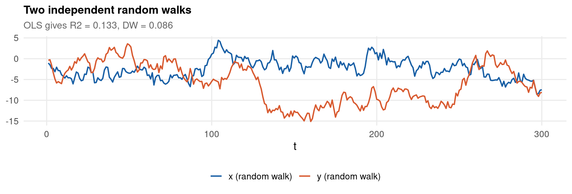
Code
import pandas as pd, matplotlib.pyplot as plt
import statsmodels.api as sm
from statsmodels.stats.stattools import durbin_watson

sim = pd.read_csv("../data/ur-vecm-sim.csv")
fit = sm.OLS(sim["y_spur"], sm.add_constant(sim["x_spur"])).fit()
r2  = fit.rsquared
dw  = durbin_watson(fit.resid)

fig, ax = plt.subplots(figsize=(10, 3.4))
ax.plot(sim["t"], sim["x_spur"], color="#185FA5", lw=1.0, label="x (random walk)")
ax.plot(sim["t"], sim["y_spur"], color="#D85A30", lw=1.0, label="y (random walk)")
ax.text(0.02, 0.06, f"R2 = {r2:.3f}   DW = {dw:.3f}   t = {fit.tvalues.iloc[1]:.2f}",
        transform=ax.transAxes, fontsize=13, color="#8b0000")
axopts = ax.set(xlabel="t", ylabel=None, title="Two independent random walks")
ax.legend(fontsize=11)
plt.tight_layout()
plt.show()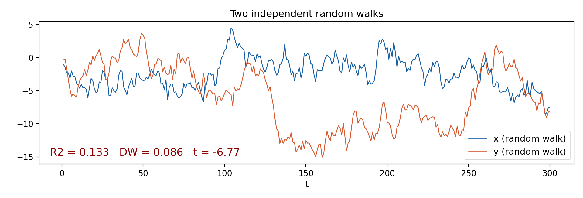
Code
      Source |       SS           df       MS      Number of obs   =       300
-------------+----------------------------------   F(1, 298)       =     45.77
       Model |  911.965431         1  911.965431   Prob > F        =    0.0000
    Residual |  5937.43928       298  19.9242929   R-squared       =    0.1331
-------------+----------------------------------   Adj R-squared   =    0.1302
       Total |  6849.40471       299   22.907708   Root MSE        =    4.4637

------------------------------------------------------------------------------
      y_spur | Coefficient  Std. err.      t    P>|t|     [95% conf. interval]
-------------+----------------------------------------------------------------
      x_spur |  -.7521165   .1111699    -6.77   0.000    -.9708941   -.5333389
       _cons |  -7.697922   .3729237   -20.64   0.000     -8.43182   -6.964024
------------------------------------------------------------------------------


Durbin–Watson d-statistic(  2,   300) =  .0862945
The three tabs analyse the same two columns of ur-vecm-sim.csv, so the coefficient, \(R^2\) and DW agree exactly across languages.
What to look at, in order:
- \(R^2\) — high, and it has no economic content whatsoever. The two series were generated independently.
- \(t\)-statistic — large. Under the usual asymptotics this would be decisive evidence. It is evidence of nothing.
- DW — close to zero, the signature of \(I(1)\) residuals. \(R^2 > DW\) is the Granger-Newbold rule of thumb firing.
More data makes it worse, not better
Re-run the simulation with \(T = 50\), \(T = 100\) and \(T = 500\). The \(R^2\) does not shrink and the \(t\)-statistic grows.
That is the point: the problem is not a small-sample artefact that more data will cure. Under the null of no cointegration the \(t\)-statistic diverges, so a larger sample buys a more confident wrong answer.
Integration Orders
A series \(\{y_t\}\) is integrated of order \(d\), written \(y_t \sim I(d)\), if it must be differenced \(d\) times to become stationary:
\[ \Delta^d y_t \sim I(0) \]
| Process | Order | Representation | ACF |
|---|---|---|---|
| White noise | \(I(0)\) | \(y_t = \varepsilon_t\) | Cuts off at lag 0 |
| Stationary AR(1) | \(I(0)\) | \(y_t = \rho y_{t-1} + \varepsilon_t\), \(\lvert\rho\rvert<1\) | Decays geometrically |
| Random walk | \(I(1)\) | \(y_t = y_{t-1} + \varepsilon_t\) | Decays very slowly |
| Random walk with drift | \(I(1)\) | \(y_t = \mu + y_{t-1} + \varepsilon_t\) | Decays very slowly |
| Double unit root | \(I(2)\) | \(\Delta^2 y_t \sim I(0)\) | Never dies |
For a random walk started at \(y_0 = 0\),
\[ y_T = \sum_{t=1}^{T}\varepsilon_t, \qquad \operatorname{Var}(y_T) = T\sigma^2 \]
Three consequences follow, and each one breaks a standard result:
- The variance grows without bound. There is no population mean to revert to, so “the mean of the series” is not a meaningful quantity.
- Shocks are permanent. \(\partial y_{t+h}/\partial \varepsilon_t = 1\) for every horizon \(h\). The impulse response never decays.
- Sample moments do not converge to constants, which is exactly why the OLS \(t\)-statistic loses its \(N(0,1)\) limit.
\[ \frac{1}{T}\sum_{t=1}^{T} y_t^2 \;\xrightarrow{d}\; \sigma^2\!\int_0^1 W(r)^2\,dr \]
The limit is a random variable — a functional of Brownian motion — not a number.
The Unit Root Hypothesis
For the AR(1) model
\[ y_t = \rho y_{t-1} + \varepsilon_t, \qquad \varepsilon_t \sim WN(0,\sigma^2) \]
the hypotheses are
\[ H_0: \rho = 1 \quad \text{(unit root, non-stationary)} \]
\[ H_1: \lvert\rho\rvert < 1 \quad \text{(stationary)} \]
Why not a standard \(t\)-test? Under \(H_0\) the OLS estimator converges at rate \(T\) rather than \(\sqrt{T}\), and its limit is not normal:
\[ T(\hat\rho - 1) \;\xrightarrow{d}\; \frac{\int_0^1 W\,dW}{\int_0^1 W^2\,dt} \]
where \(W(\cdot)\) is standard Brownian motion. The distribution is skewed to the left, so the critical values are negative and must be obtained by simulation — this is what Dickey and Fuller tabulated.
One problem, restated in every test of Part II
Every test in Part II is a variation on this single problem: how to get a usable critical value for \(\hat\rho - 1\) when the null makes the regressor non-stationary.
The tests differ in how they buy back power — augmentation, a kernel correction, GLS detrending, a break search — but the obstacle they are working around is always this one.
DGP — Mathematical Specification
Five series with known integration order, plus a cointegrated pair, all with \(\varepsilon_t \sim N(0,1)\) and seed 14159.
\(I(0)\) — stationary AR(1):
\[ y_t^{(0)} = 0.6\,y_{t-1}^{(0)} + \varepsilon_t \]
\(I(1)\) — pure random walk:
\[ y_t^{(1)} = y_{t-1}^{(1)} + \varepsilon_t, \qquad y_0^{(1)} = 0 \]
\(I(1)\) with drift:
\[ y_t^{(d)} = 0.3 + y_{t-1}^{(d)} + \varepsilon_t \]
\(I(2)\) — double unit root:
\[ y_t^{(2)} = 2y_{t-1}^{(2)} - y_{t-2}^{(2)} + \varepsilon_t \]
Cointegrated pair, true \(\beta = 2\):
\[ x_t = x_{t-1} + v_t, \qquad y_t^{(c)} = 2x_t + u_t, \qquad u_t = 0.4u_{t-1} + \eta_t \]
Because \(u_t\) is a stationary AR(1), the combination \(y_t^{(c)} - 2x_t\) is \(I(0)\) by construction: the pair is cointegrated with cointegrating vector \([1, -2]'\) and the error correction term is \(u_t\).
DGP Diagnostics
Code
sim_df <- read.csv("../data/ur-vecm-sim.csv")

p_paths <- sim_df |>
  select(t, i0, i1, i1d) |>
  pivot_longer(-t, names_to = "series", values_to = "value") |>
  mutate(series = factor(series, levels = c("i0", "i1", "i1d"),
                         labels = c("I(0): AR(1)", "I(1): random walk",
                                    "I(1) with drift"))) |>
  ggplot() +
  aes(t, value, colour = series) +
  geom_line(linewidth = 0.6) +
  facet_wrap(~series, scales = "free_y", ncol = 1) +
  scale_colour_manual(values = c("#185FA5", "#D85A30", "#1D9E75")) +
  labs(title = "Time paths by integration order", x = "t", y = NULL) +
  theme_lecture + theme(legend.position = "none")

p_coint <- sim_df |>
  mutate(spread = y_c - 2 * x_c) |>
  ggplot() +
  aes(t, spread) +
  geom_line(colour = "#BA7517", linewidth = 0.7) +
  geom_hline(yintercept = 0, linetype = "dashed") +
  labs(title = "Cointegrating residual  y_c - 2 x_c",
       subtitle = "I(0) by construction", x = "t", y = NULL) +
  theme_lecture

p_paths + p_coint + plot_layout(ncol = 2)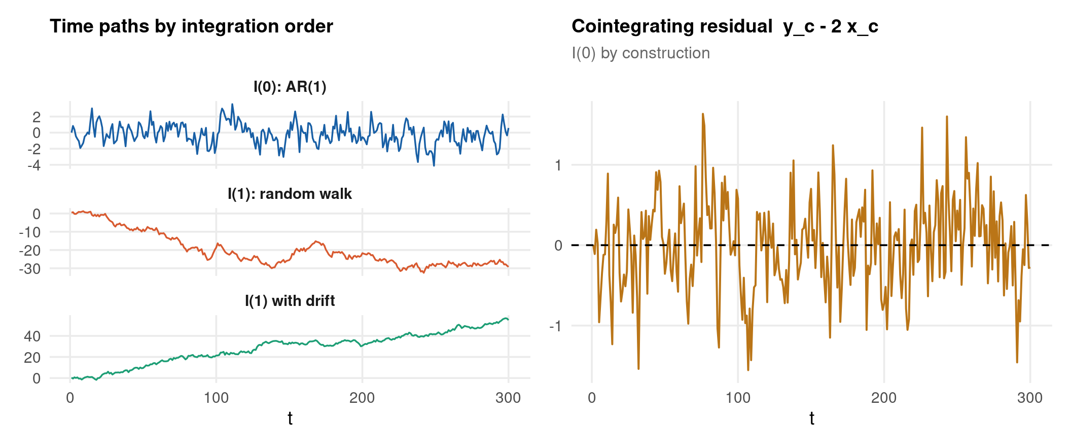
Code
import pandas as pd, matplotlib.pyplot as plt

sim = pd.read_csv("../data/ur-vecm-sim.csv")
fig, axes = plt.subplots(2, 2, figsize=(11, 4.6))
panels = [("i0",  "I(0): AR(1)",        "#185FA5"),
          ("i1",  "I(1): random walk",  "#D85A30"),
          ("i1d", "I(1) with drift",    "#1D9E75"),
          (None,  "Cointegrating residual  y_c - 2 x_c", "#BA7517")]
for ax, (col, title, clr) in zip(axes.flat, panels):
    if col:
        ax.plot(sim["t"], sim[col], color=clr, lw=0.8)
    else:
        ax.plot(sim["t"], sim["y_c"] - 2 * sim["x_c"], color=clr, lw=0.8)
        ax.axhline(0, ls="--", color="grey")
    axopts = ax.set(title=title, xlabel="t")
    ax.title.set_fontsize(10)
plt.tight_layout()
plt.show()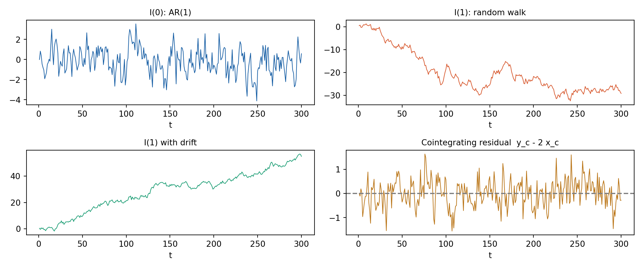
Code
quietly import delimited "../data/ur-vecm-sim.csv", clear
quietly destring _all, replace
quietly tsset t
quietly gen spread = y_c - 2*x_c
summarize i0 i1 i1d i2 spread, separator(0)
display ""
display "Autocorrelation at lag 1 (I(0) decays fast, I(1) does not):"
foreach v in i0 i1 i1d {
    quietly corrgram `v', lags(1)
    display "  `v': AC(1) = " %6.4f r(ac1)
}
Variable | Obs Mean Std. dev. Min Max
-------------+---------------------------------------------------------
i0 | 300 -.1754977 1.277084 -4.120092 3.54809
i1 | 300 -19.97237 9.050471 -32.48036 1.264598
i1d | 300 28.36648 14.86497 -1.719559 56.76815
i2 | 300 1278.386 613.4979 1.367044 2054.983
spread | 300 .0005113 .5604704 -1.554247 1.633341
Autocorrelation at lag 1 (I(0) decays fast, I(1) does not):
i0: AC(1) = 0.5874
i1: AC(1) = 0.9838
i1d: AC(1) = 0.9865The three panels on the left show what integration order looks like before any test is run.
- \(I(0)\) oscillates around a fixed level and crosses its mean repeatedly.
- \(I(1)\) wanders. It has no level to return to, and long excursions away from zero are normal rather than exceptional.
- \(I(1)\) with drift adds a deterministic slope on top of the wandering, which is why the ADF specification with a trend matters.
The right-hand panel is the whole idea of cointegration in one picture: y_c and x_c are each \(I(1)\) and neither reverts, but the specific combination \(y_c - 2x_c\) does. The summary statistics in the Stata tab make the same point numerically — the first-order autocorrelation is near 0.6 for the \(I(0)\) series and close to 1 for both \(I(1)\) series.
Part II — Unit Root Tests
τί χρῆμα δόξης; τοῦ δʼ ἔχεις τεκμήριον;
what is this opinion? what proof have you of it?
Εὐριπίδης, Ἡρακλῆς 714
Augmented Dickey-Fuller
Regression with intercept and trend:
\[ \Delta y_t = \alpha + \delta t + \gamma y_{t-1} + \sum_{j=1}^{p}\theta_j \Delta y_{t-j} + \varepsilon_t \]
\[ H_0: \gamma = 0 \quad \text{(unit root)} \qquad H_1: \gamma < 0 \quad \text{(stationary)} \]
\[ \tau = \frac{\hat\gamma}{\operatorname{SE}(\hat\gamma)} \]
Reject \(H_0\) when \(\tau < \tau_{\text{crit}}\). This is a left-tail test and the critical values are negative.
The lagged differences \(\Delta y_{t-j}\) are the “augmentation”: they soak up serial correlation so that \(\varepsilon_t\) is white noise, which is what the tabulated distribution assumes.
| Spec | Intercept | Trend | Use when |
|---|---|---|---|
trend |
Yes | Yes | The series visibly trends |
drift |
Yes | No | Wanders around a non-zero mean, no trend |
none |
No | No | Centred at zero — in practice only for residuals |
Under-specifying the deterministic terms
Choosing drift for a trending series under-specifies the regression and biases the test toward rejecting the unit root.
Plot the series first, every time. The deterministic specification is part of the null being tested, not a display option.
Lag selection. Too few lags leaves serial correlation in the residuals and oversizes the test; too many costs power. AIC is the usual default; the Schwert rule \(p_{\max} = \lfloor 12(T/100)^{1/4}\rfloor\) sets a sensible upper bound.
summary(ur.df(...)) prints tau3 (the \(t\)-statistic on the lagged level with a trend) together with phi2 and phi3, which are joint \(F\)-tests on the deterministic terms. For the unit-root decision only tau3 matters:
tau3 statistic:   -2.14
Critical values:  1pct -4.04   5pct -3.45   10pct -3.15
  -2.14 > -3.45  ->  fail to reject H0  ->  the level looks I(1)
Then test the first difference, with type = "drift" because differencing removes the trend:
tau2 statistic:   -7.32
Critical values:  5pct -2.89
  -7.32 < -2.89  ->  reject H0  ->  the difference is I(0)  ->  the series is I(1)
Two rejections in that order is what “the series is \(I(1)\)” actually means. A single failure to reject on the level proves nothing on its own — it is equally consistent with \(I(2)\).
ADF — Code
Code
sim_df <- read.csv("../data/ur-vecm-sim.csv")

# tseries: quick p-value, Schwert lag rule
adf_i0 <- tseries::adf.test(sim_df$i0)
adf_i1 <- tseries::adf.test(sim_df$i1)
print(adf_i0); print(adf_i1)

# urca: full regression table and the choice of specification
ur_i1 <- urca::ur.df(sim_df$i1, type = "trend", lags = 4, selectlags = "AIC")
summary(ur_i1)
--- ADF on the I(0) series ---
    Augmented Dickey-Fuller Test

data:  sim_df$i0
Dickey-Fuller = -5.6571, Lag order = 6, p-value = 0.01
alternative hypothesis: stationary
--- ADF on the I(1) series ---
    Augmented Dickey-Fuller Test

data:  sim_df$i1
Dickey-Fuller = -2.0079, Lag order = 6, p-value = 0.573
alternative hypothesis: stationary
--- urca::ur.df, trend specification, I(1) series ---tau3 = -2.2900 critical values: 1pct -3.98 5pct -3.42 10pct -3.13Differenced: tau2 = -8.3727 5pct = -2.87 -> reject, difference is I(0), series is I(1)Code
import pandas as pd
from statsmodels.tsa.stattools import adfuller

sim = pd.read_csv("../data/ur-vecm-sim.csv")
lines = []
for col, label in [("i0", "I(0)"), ("i1", "I(1)")]:
    res = adfuller(sim[col], autolag="AIC", regression="ct")
    lines.append(f"--- ADF on {label} ({col}) ---")
    lines.append(f"  statistic : {res[0]:.4f}")
    lines.append(f"  p-value   : {res[1]:.4f}")
    lines.append(f"  lags used : {res[2]}")
    for k, v in res[4].items():
        lines.append(f"  CV {k:>3} : {v:.4f}")
    lines.append("  verdict   : " + ("reject H0 (stationary)" if res[1] < 0.05
                                     else "fail to reject H0 (unit root)"))

d = adfuller(sim["i1"].diff().dropna(), autolag="AIC", regression="c")
lines.append(f"\nFirst difference of i1: stat = {d[0]:.4f}, p = {d[1]:.4f}")

out = "\n".join(lines)
import sys; sys.stdout.write(out + "\n"); sys.stdout.flush()
--- ADF on I(0) (i0) ---
statistic : -8.9543
p-value : 0.0000
lags used : 0
CV 1% : -3.9894
CV 5% : -3.4253
CV 10% : -3.1357
verdict : reject H0 (stationary)
--- ADF on I(1) (i1) ---
statistic : -2.1344
p-value : 0.5268
lags used : 5
CV 1% : -3.9899
CV 5% : -3.4255
CV 10% : -3.1359
verdict : fail to reject H0 (unit root)
First difference of i1: stat = -8.3727, p = 0.0000
415Code
quietly import delimited "../data/ur-vecm-sim.csv", clear
quietly destring _all, replace
quietly tsset t
display "--- ADF on the I(0) series ---"
dfuller i0, trend lags(4)
display "--- ADF on the I(1) series ---"
dfuller i1, trend lags(4)
display "--- ADF on the first difference of the I(1) series ---"
dfuller D.i1, lags(4)
--- ADF on the I(0) series ---
Augmented Dickey–Fuller test for unit root
Variable: i0 Number of obs = 295
Number of lags = 4
H0: Random walk with or without drift
Dickey–Fuller
Test -------- critical value ---------
statistic 1% 5% 10%
--------------------------------------------------------------
Z(t) -5.661 -3.988 -3.428 -3.130
--------------------------------------------------------------
MacKinnon approximate p-value for Z(t) = 0.0000.
--- ADF on the I(1) series ---
Augmented Dickey–Fuller test for unit root
Variable: i1 Number of obs = 295
Number of lags = 4
H0: Random walk with or without drift
Dickey–Fuller
Test -------- critical value ---------
statistic 1% 5% 10%
--------------------------------------------------------------
Z(t) -2.254 -3.988 -3.428 -3.130
--------------------------------------------------------------
MacKinnon approximate p-value for Z(t) = 0.4598.
--- ADF on the first difference of the I(1) series ---
Augmented Dickey–Fuller test for unit root
Variable: D.i1 Number of obs = 294
Number of lags = 4
H0: Random walk without drift, d = 0
Dickey–Fuller
Test -------- critical value ---------
statistic 1% 5% 10%
--------------------------------------------------------------
Z(t) -8.373 -3.456 -2.878 -2.570
--------------------------------------------------------------
MacKinnon approximate p-value for Z(t) = 0.0000.The known truth: i0 is a stationary AR(1) with \(\rho = 0.6\) and i1 is a pure random walk. A test that works should reject on i0 and fail to reject on i1 — and all three languages do exactly that on the same data.
The last line of each tab is the confirmation step. Differencing i1 produces a series on which the test rejects decisively, which is what pins the order at \(I(1)\) rather than \(I(2)\).
Interpolated p-values or tabulated critical values
tseries::adf.test and statsmodels.adfuller report an interpolated \(p\)-value; urca::ur.df and Stata’s dfuller report the statistic against tabulated critical values.
Both are the same test — only the presentation differs. Compare statistics with statistics across the three tabs, never a \(p\)-value in one against a critical value in another.
Phillips-Perron
\[ \Delta y_t = \alpha + \delta t + \gamma y_{t-1} + u_t \]
Phillips-Perron adds no lagged differences. Instead it corrects the statistic non-parametrically for whatever serial correlation is in \(u_t\), using the long-run variance
\[ \hat\omega^2 = \hat\sigma^2 + 2\sum_{j=1}^{l}\left(1 - \frac{j}{l+1}\right)\hat\gamma_j \]
\[ Z_\tau = \tau_{\hat\gamma}\cdot\frac{\hat\sigma}{\hat\omega} \;-\; \frac{T(\hat\omega^2 - \hat\sigma^2)}{2\hat\omega\sqrt{S_{11}}} \]
The limiting distribution is the same as the ADF, so the same critical values apply.
| ADF | PP | |
|---|---|---|
| Serial correlation | Parametric, via lagged differences | Non-parametric, via a kernel |
| Heteroscedastic errors | Sensitive | More robust |
| MA errors with root near \(-1\) | Size distortion | Severe size distortion |
| Small samples | Reasonable | Can over-reject |
PP is a second opinion, not a replacement
PP is not a replacement for ADF, it is a second opinion with a different weakness.
When they disagree, the Ng-Perron M-tests later in this part are designed for exactly that case.
Phillips-Perron — Code
--- PP on the I(0) series ---
    Phillips-Perron Unit Root Test

data:  sim_df$i0
Dickey-Fuller Z(alpha) = -126.38, Truncation lag parameter = 5, p-value
= 0.01
alternative hypothesis: stationary
--- PP on the I(1) series ---
    Phillips-Perron Unit Root Test

data:  sim_df$i1
Dickey-Fuller Z(alpha) = -8.1306, Truncation lag parameter = 5, p-value
= 0.6545
alternative hypothesis: stationary
urca::ur.pp Z-tau = -2.0987 5pct critical value = -3.43Code
import pandas as pd
from arch.unitroot import PhillipsPerron

sim = pd.read_csv("../data/ur-vecm-sim.csv")
lines = []
for col, label in [("i0", "I(0)"), ("i1", "I(1)")]:
    pp = PhillipsPerron(sim[col], trend="ct")
    lines.append(f"--- PP on {label} ({col}) ---")
    lines.append(f"  statistic : {pp.stat:.4f}")
    lines.append(f"  p-value   : {pp.pvalue:.4f}")
    lines.append(f"  lags      : {pp.lags}")
    lines.append("  verdict   : " + ("reject H0" if pp.pvalue < 0.05
                                     else "fail to reject H0"))
out = "\n".join(lines)
import sys; sys.stdout.write(out + "\n"); sys.stdout.flush()
--- PP on I(0) (i0) ---
statistic : -8.5930
p-value : 0.0000
lags : 16
verdict : reject H0
--- PP on I(1) (i1) ---
statistic : -1.9790
p-value : 0.6128
lags : 16
verdict : fail to reject H0
224Code
--- PP on the I(0) series ---


Phillips–Perron test for unit root       Number of obs   = 299
Variable: i0                             Newey–West lags =   6

H0: Random walk with or without drift

                                       Dickey–Fuller
                   Test      -------- critical value ---------
              statistic           1%           5%          10%
--------------------------------------------------------------
 Z(rho)        -127.165      -28.498      -21.339      -18.020
 Z(t)            -8.935       -3.988       -3.428       -3.130
--------------------------------------------------------------
MacKinnon approximate p-value for Z(t) = 0.0000.

--- PP on the I(1) series ---


Phillips–Perron test for unit root       Number of obs   = 299
Variable: i1                             Newey–West lags =   6

H0: Random walk with or without drift

                                       Dickey–Fuller
                   Test      -------- critical value ---------
              statistic           1%           5%          10%
--------------------------------------------------------------
 Z(rho)          -7.888      -28.498      -21.339      -18.020
 Z(t)            -2.098       -3.988       -3.428       -3.130
--------------------------------------------------------------
MacKinnon approximate p-value for Z(t) = 0.5471.
KPSS
KPSS reverses the null: stationarity is \(H_0\), a unit root is \(H_1\).
\[ y_t = \xi t + r_t + \varepsilon_t, \qquad r_t = r_{t-1} + u_t, \qquad u_t \sim WN(0,\sigma_u^2) \]
Under \(H_0\), \(\sigma_u^2 = 0\): the random-walk component vanishes and the series is stationary around its deterministic part.
\[ \eta_\mu = \frac{1}{T^2\hat\omega^2}\sum_{t=1}^{T}S_t^2, \qquad S_t = \sum_{j=1}^{t}\hat\varepsilon_j \]
Reject \(H_0\) when \(\eta > \eta_{\text{crit}}\). This is a right-tail test — the opposite direction from ADF and PP.
The reason to run KPSS at all is that it fails in a different direction from ADF, so the pair of results is more informative than either alone.
| ADF | KPSS | Conclusion |
|---|---|---|
| Fail to reject | Reject | \(I(1)\) confirmed |
| Reject | Fail to reject | \(I(0)\) confirmed |
| Fail to reject | Fail to reject | Ambiguous — low power, try DF-GLS |
| Reject | Reject | Contradictory — suspect a structural break |
Failing to reject is not evidence for the null
Failing to reject is not evidence for a null. Unit root tests have notoriously low power against \(\rho = 0.95\).
That is why the confirmatory pairing exists — and why the bottom two rows of the table are common in practice rather than rare.
KPSS — Code
--- KPSS on the I(0) series ---
    KPSS Test for Level Stationarity

data:  sim_df$i0
KPSS Level = 0.48214, Truncation lag parameter = 5, p-value = 0.04569
--- KPSS on the I(1) series ---
    KPSS Test for Level Stationarity

data:  sim_df$i1
KPSS Level = 3.7738, Truncation lag parameter = 5, p-value = 0.01
urca::ur.kpss eta = 1.4985 5pct critical value = 0.463 -> reject stationarityCode
import pandas as pd, warnings
warnings.filterwarnings("ignore")
from statsmodels.tsa.stattools import kpss

sim = pd.read_csv("../data/ur-vecm-sim.csv")
lines = []
for col, label in [("i0", "I(0)"), ("i1", "I(1)")]:
    stat, pval, lags, cv = kpss(sim[col], regression="c", nlags="auto")
    lines.append(f"--- KPSS on {label} ({col}) ---")
    lines.append(f"  statistic : {stat:.4f}")
    lines.append(f"  p-value   : {pval:.4f}")
    for k, v in cv.items():
        lines.append(f"  CV {k:>4} : {v:.4f}")
    lines.append("  verdict   : " + ("reject H0 (not stationary)" if pval < 0.05
                                     else "fail to reject H0 (stationary)"))
out = "\n".join(lines)
import sys; sys.stdout.write(out + "\n"); sys.stdout.flush()
--- KPSS on I(0) (i0) ---
statistic : 0.4217
p-value : 0.0678
CV 10% : 0.3470
CV 5% : 0.4630
CV 2.5% : 0.5740
CV 1% : 0.7390
verdict : fail to reject H0 (stationary)
--- KPSS on I(1) (i1) ---
statistic : 2.1192
p-value : 0.0100
CV 10% : 0.3470
CV 5% : 0.4630
CV 2.5% : 0.5740
CV 1% : 0.7390
verdict : reject H0 (not stationary)
374Code
--- KPSS on the I(0) series ---


KPSS test for i0

Maxlag = 15 chosen by Schwert criterion
Autocovariances weighted by Bartlett kernel

Critical values for H0: i0 is trend stationary

10%: 0.119  5% : 0.146  2.5%: 0.176  1% : 0.216

Lag order    Test statistic
    0          .0931
    1          .0593
    2          .0474
    3          .0414
    4           .038
    5          .0357
    6          .0341
    7           .033
    8          .0322
    9          .0319
   10          .0318
   11          .0318
   12           .032
   13          .0323
   14          .0327
   15          .0332

--- KPSS on the I(1) series ---


KPSS test for i1

Maxlag = 15 chosen by Schwert criterion
Autocovariances weighted by Bartlett kernel

Critical values for H0: i1 is trend stationary

10%: 0.119  5% : 0.146  2.5%: 0.176  1% : 0.216

Lag order    Test statistic
    0           4.28
    1           2.17
    2           1.46
    3           1.11
    4           .896
    5           .755
    6           .654
    7           .579
    8            .52
    9           .473
   10           .435
   11           .402
   12           .375
   13           .352
   14           .332
   15           .314
DF-GLS
Elliott, Rothenberg & Stock (1996): remove the deterministic part by GLS before running the Dickey-Fuller regression. The gain in power against near-unit-root alternatives is large.
Step 1 — quasi-difference with \(\bar\alpha = 1 + \bar c/T\) and regress:
\[ \tilde y_t = y_t - \hat\delta' z_t \]
with \(z_t = (1,t)'\) and \(\bar c = -13.5\) in the trend case, \(\bar c = -7\) with a constant only.
Step 2 — ADF on the detrended series, no deterministic terms:
\[ \Delta\tilde y_t = \gamma\tilde y_{t-1} + \sum_{j=1}^{p}\theta_j\Delta\tilde y_{t-j} + \varepsilon_t \]
\[ H_0: \gamma = 0 \qquad H_1: \gamma < 0 \]
Estimating an intercept and trend by OLS costs power, because under the null those estimates are contaminated by the stochastic trend. GLS detrending at a local alternative \(\rho = 1 + \bar c/T\) estimates them under conditions close to where the power actually matters.
The result is a test with near-optimal power in the sense of the Neyman-Pearson envelope. In practice: DF-GLS rejects at \(\rho = 0.95\) where ADF frequently does not.
Why DF-GLS should be the default
When power matters — and with macro series of 100–300 observations it always does — DF-GLS is the better default than plain ADF.
The cost is nothing but a different set of critical values, which every implementation already carries.
DF-GLS — Code
     Series Statistic CV_1pct CV_5pct CV_10pct        Verdict
 i0  (I(0))   -5.4637   -3.48   -2.89    -2.57      reject H0
 i1  (I(1))   -1.1687   -3.48   -2.89    -2.57 fail to reject
Code
import pandas as pd
from arch.unitroot import DFGLS

sim = pd.read_csv("../data/ur-vecm-sim.csv")
lines = []
for col, label in [("i0", "I(0)"), ("i1", "I(1)")]:
    t = DFGLS(sim[col], trend="ct", max_lags=8)
    lines.append(f"--- DF-GLS on {label} ({col}) ---")
    lines.append(f"  statistic : {t.stat:.4f}")
    lines.append(f"  p-value   : {t.pvalue:.4f}")
    lines.append(f"  lags      : {t.lags}")
    lines.append("  verdict   : " + ("reject H0" if t.pvalue < 0.05
                                     else "fail to reject H0"))
out = "\n".join(lines)
import sys; sys.stdout.write(out + "\n"); sys.stdout.flush()
--- DF-GLS on I(0) (i0) ---
statistic : -8.8972
p-value : 0.0000
lags : 0
verdict : reject H0
--- DF-GLS on I(1) (i1) ---
statistic : -1.3075
p-value : 0.6906
lags : 5
verdict : fail to reject H0
230Code
--- DF-GLS on the I(0) series ---


DF-GLS test for unit root                  Number of obs = 291
Variable: i0
Lag selection: User specified              Maximum lag   =   8

                             -------- Critical value ---------
 [lags]      DF-GLS tau           1%           5%          10%
--------------------------------------------------------------
      8          -5.464       -3.480       -2.864       -2.579
      7          -5.398       -3.480       -2.870       -2.585
      6          -5.507       -3.480       -2.876       -2.590
      5          -5.705       -3.480       -2.882       -2.595
      4          -5.617       -3.480       -2.887       -2.600
      3          -6.899       -3.480       -2.892       -2.605
      2          -7.102       -3.480       -2.897       -2.609
      1          -8.084       -3.480       -2.902       -2.613
--------------------------------------------------------------
Opt lag (Ng–Perron seq t) = 4 with RMSE =  1.02764
Min SIC  =  .1131372 at lag 1 with RMSE = 1.037768
Min MAIC =  .5458488 at lag 4 with RMSE =  1.02764

--- DF-GLS on the I(1) series ---


DF-GLS test for unit root                  Number of obs = 291
Variable: i1
Lag selection: User specified              Maximum lag   =   8

                             -------- Critical value ---------
 [lags]      DF-GLS tau           1%           5%          10%
--------------------------------------------------------------
      8          -1.169       -3.480       -2.864       -2.579
      7          -1.090       -3.480       -2.870       -2.585
      6          -1.180       -3.480       -2.876       -2.590
      5          -1.307       -3.480       -2.882       -2.595
      4          -1.520       -3.480       -2.887       -2.600
      3          -1.681       -3.480       -2.892       -2.605
      2          -1.548       -3.480       -2.897       -2.609
      1          -1.379       -3.480       -2.902       -2.613
--------------------------------------------------------------
Opt lag (Ng–Perron seq t) = 5 with RMSE = .9669869
Min SIC  =   .005039 at lag 1 with RMSE = .9831668
Min MAIC = -.0200611 at lag 5 with RMSE = .9669869
Zivot-Andrews
The problem. A one-off level shift in a stationary series looks like a unit root to the ADF test. Perron (1989) showed that ignoring a known break biases the test badly toward failing to reject.
The fix. Zivot & Andrews (1992) treat the break date as unknown and search for it:
\[ \Delta y_t = c + \beta t + \alpha y_{t-1} + \gamma DU_t(\lambda) + \psi DT_t(\lambda) + \sum_{j=1}^{k}\theta_j\Delta y_{t-j} + \varepsilon_t \]
with \(DU_t(\lambda)=\mathbf{1}[t > \lambda T]\) a level break and \(DT_t(\lambda) = t\cdot\mathbf{1}[t > \lambda T]\) a trend break.
\[ ZA = \inf_{\lambda\in\Lambda} t_{\hat\alpha}(\lambda) \]
The statistic is the minimum \(t\)-statistic over all candidate break fractions in a trimmed range, so its critical values are far more negative than the ADF ones.
- The break is under \(H_1\), not \(H_0\). Rejecting means “stationary around a broken trend”, not “there is a break”.
- Because the search takes an infimum, using ADF critical values would reject far too often.
- With a break under the null as well, the ZA test over-rejects; Lee & Strazicich (2003) is the usual remedy.
- The estimated break date is only informative when the rejection is decisive.
Trimming is not a detail
Trimming matters. The standard 15% at each end exists because a “break” in the first or last few observations is indistinguishable from an outlier.
Change the trimming and the infimum is taken over a different set, so the critical values no longer apply.
Zivot-Andrews — Code
--- Zivot-Andrews on the I(1) series, break in level and trend --- minimum t-statistic : -4.5895 break at observation: 140 of 300 critical values : 1pct -5.57 5pct -5.08 10pct -4.82 verdict : fail to reject H0 - unit root survives the break allowanceCode
import numpy as np, pandas as pd
from arch.unitroot import ZivotAndrews

sim = pd.read_csv("../data/ur-vecm-sim.csv")
# method selects the lag length: "aic", "bic" or "t-stat". There is no
# "both" option here - arch always allows a break in level and trend for
# trend="ct".
za = ZivotAndrews(sim["i1"], trend="ct", method="aic")
za.stat-4.21266964071403Code
# arch computes the statistic at every candidate break but exposes only the
# minimum, so recover the break date from the stored grid.
grid  = np.asarray(za._all_stats)
brk   = int(np.nanargmin(grid)) + 1

lines = ["--- Zivot-Andrews on the I(1) series ---",
         f"  minimum t-statistic : {za.stat:.4f}",
         f"  p-value             : {za.pvalue:.4f}",
         f"  break at observation: {brk} of {len(sim)}",
         f"  lags                : {za.lags}",
         "  verdict             : " + ("reject H0" if za.pvalue < 0.05
                                       else "fail to reject H0")]
out = "\n".join(lines)
import sys; sys.stdout.write(out + "\n"); sys.stdout.flush()
--- Zivot-Andrews on the I(1) series ---
minimum t-statistic : -4.2127
p-value : 0.3659
break at observation: 141 of 300
lags : 5
verdict : fail to reject H0
207Code
Zivot-Andrews unit root test for  i1

Allowing for break in both intercept and trend

Lag selection via AIC: lags of D.i1 included = 0

Minimum t-statistic -4.290 at 141  (obs 141)

Critical values: 1%: -5.57 5%: -5.08 10%: -4.82
The series is a pure random walk with no break anywhere in it, so the correct answer is fail to reject — and all three tabs give that.
This is the useful case to see first. A test that searches 70% of the sample for the most favourable break date and still cannot reject is telling you the persistence is real, not an artefact of a level shift. Had the test rejected here it would have been a false positive, which is precisely the risk that the more negative critical values are there to control.
The break date the search lands on is meaningful only under rejection. Here it is simply the point where a spurious shift fits best, and it should not be reported as if the series had broken there.
Ng-Perron M-Tests
Ng & Perron (2001) combine GLS detrending with modified M-statistics, aimed at the case where the errors have a moving-average root near \(-1\) — the configuration in which ADF and especially PP suffer severe size distortion.
From the GLS-detrended series \(\tilde y_t\) with long-run variance \(\hat\omega^2\):
\[ MZ_\alpha^{GLS} = \frac{T^{-1}\tilde y_T^2 - \hat\omega^2}{2T^{-2}\sum_{t}\tilde y_{t-1}^2} \]
\[ MSB^{GLS} = \left(\frac{T^{-2}\sum_t \tilde y_{t-1}^2}{\hat\omega^2}\right)^{1/2}, \qquad MZ_t^{GLS} = MZ_\alpha^{GLS}\cdot MSB^{GLS} \]
\[ MP_T^{GLS} = \frac{\bar c^{\,2}T^{-2}\sum_t\tilde y_{t-1}^2 - \bar c\,T^{-1}\tilde y_T^2}{\hat\omega^2} \quad \text{(trend case)} \]
\(MZ_\alpha\), \(MZ_t\) and \(MSB\) reject for small values; \(MP_T\) is a point-optimal statistic and also rejects for small values.
Trend case, \(\bar c = -13.5\), from Ng & Perron (2001) Table 1:
| Statistic | 1% | 5% | 10% |
|---|---|---|---|
| \(MZ_\alpha\) | \(-23.8\) | \(-17.3\) | \(-14.2\) |
| \(MZ_t\) | \(-3.42\) | \(-2.91\) | \(-2.62\) |
| \(MSB\) | \(0.143\) | \(0.168\) | \(0.185\) |
| \(MP_T\) | \(4.03\) | \(5.48\) | \(6.67\) |
Constant-only case, \(\bar c = -7\): \(MZ_\alpha\) \(-8.10\), \(MZ_t\) \(-1.98\), \(MSB\) \(0.233\), \(MP_T\) \(3.17\) at 5%.
No package ships the M-tests
No R package exports these tests, statsmodels and arch do not implement them, and Stata’s dfgls reports the DF-GLS \(\tau\) rather than the M-statistics.
The next slide therefore codes them from the definitions above — the same twenty lines in all three languages, which is also the cleanest way to see what the statistics actually are.
Ng-Perron — Code
Code
ng_perron <- function(y, model = c("trend", "constant"), lag_max = 8) {
  model <- match.arg(model)
  n  <- length(y)
  cb <- if (model == "trend") -13.5 else -7
  ab <- 1 + cb / n
  z  <- if (model == "trend") cbind(1, seq_len(n)) else cbind(rep(1, n))
  # quasi-difference the data and the deterministic terms, then detrend by GLS
  yq <- c(y[1], y[-1] - ab * y[-n])
  zq <- rbind(z[1, ], z[-1, , drop = FALSE] - ab * z[-n, , drop = FALSE])
  yd <- as.numeric(y - z %*% qr.solve(zq, yq))
  dy <- diff(yd)
  # long-run variance from an autoregression, lag length by BIC
  best <- NULL
  for (k in 0:lag_max) {
    X <- cbind(yd[-n])
    if (k > 0) for (j in 1:k) X <- cbind(X, c(rep(NA, j), dy[seq_len(n - 1 - j)]))
    ok  <- complete.cases(X)
    fit <- lm.fit(X[ok, , drop = FALSE], dy[ok])
    s2  <- sum(fit$residuals^2) / length(fit$residuals)
    bic <- log(s2) + (k + 1) * log(length(fit$residuals)) / length(fit$residuals)
    if (is.null(best) || bic < best$bic)
      best <- list(k = k, bic = bic, s2 = s2, b = fit$coefficients)
  }
  sum_b <- if (best$k > 0) sum(best$b[-1]) else 0
  w2    <- best$s2 / (1 - sum_b)^2
  kap   <- sum(yd[-n]^2) / n^2
  mza   <- (yd[n]^2 / n - w2) / (2 * kap)
  msb   <- sqrt(kap / w2)
  mpt   <- if (model == "trend") (cb^2 * kap - cb * yd[n]^2 / n) / w2
           else                  (cb^2 * kap + (1 - cb) * yd[n]^2 / n) / w2
  c(MZa = mza, MZt = mza * msb, MSB = msb, MPT = mpt, lags = best$k)
}

round(ng_perron(sim_df$i0, "trend"), 4)
round(ng_perron(sim_df$i1, "trend"), 4)
Series MZa MZt MSB MPT
i0 (I(0)) -99.9697 -7.0617 0.0706 0.9411
i1 (I(1)) -3.8681 -1.3077 0.3381 22.3927
5% critical value -17.3000 -2.9100 0.1680 5.4800
Reject the unit root when MZa, MZt, MSB and MPT are all below the 5% value. i0: reject (correct, the truth is I(0)) i1: fail to reject (correct, the truth is I(1))Code
import numpy as np, pandas as pd

def ng_perron(y, model="trend", lag_max=8):
    y = np.asarray(y, float); n = y.size
    cb = -13.5 if model == "trend" else -7.0
    ab = 1 + cb / n
    z  = (np.column_stack([np.ones(n), np.arange(1, n + 1)])
          if model == "trend" else np.ones((n, 1)))
    yq = np.r_[y[0], y[1:] - ab * y[:-1]]
    zq = np.vstack([z[0], z[1:] - ab * z[:-1]])
    yd = y - z @ np.linalg.lstsq(zq, yq, rcond=None)[0]
    dy = np.diff(yd)
    best = None
    for k in range(lag_max + 1):
        cols = [yd[:-1][k:]]
        for j in range(1, k + 1):
            cols.append(dy[k - j:-j])
        X = np.column_stack(cols); yy = dy[k:]
        b, *_ = np.linalg.lstsq(X, yy, rcond=None)
        e  = yy - X @ b
        s2 = (e @ e) / e.size
        bic = np.log(s2) + (k + 1) * np.log(e.size) / e.size
        if best is None or bic < best[0]:
            best = (bic, k, s2, b)
    _, k, s2, b = best
    sum_b = b[1:].sum() if k > 0 else 0.0
    w2  = s2 / (1 - sum_b) ** 2
    kap = (yd[:-1] ** 2).sum() / n ** 2
    mza = (yd[-1] ** 2 / n - w2) / (2 * kap)
    msb = np.sqrt(kap / w2)
    mpt = ((cb ** 2 * kap - cb * yd[-1] ** 2 / n) / w2 if model == "trend"
           else (cb ** 2 * kap + (1 - cb) * yd[-1] ** 2 / n) / w2)
    return dict(MZa=mza, MZt=mza * msb, MSB=msb, MPT=mpt, lags=k)

sim = pd.read_csv("../data/ur-vecm-sim.csv")
r0, r1 = ng_perron(sim["i0"]), ng_perron(sim["i1"])
lines = [f"{'Series':<20}{'MZa':>12}{'MZt':>10}{'MSB':>10}{'MPT':>10}",
         f"{'i0  (I(0))':<20}{r0['MZa']:>12.4f}{r0['MZt']:>10.4f}"
         f"{r0['MSB']:>10.4f}{r0['MPT']:>10.4f}",
         f"{'i1  (I(1))':<20}{r1['MZa']:>12.4f}{r1['MZt']:>10.4f}"
         f"{r1['MSB']:>10.4f}{r1['MPT']:>10.4f}",
         f"{'5% critical value':<20}{-17.3:>12.4f}{-2.91:>10.4f}"
         f"{0.168:>10.4f}{5.48:>10.4f}"]
out = "\n".join(lines)
import sys; sys.stdout.write(out + "\n"); sys.stdout.flush()
Series MZa MZt MSB MPT
i0 (I(0)) -99.9697 -7.0617 0.0706 0.9411
i1 (I(1)) -3.8681 -1.3077 0.3381 22.3927
5% critical value -17.3000 -2.9100 0.1680 5.4800
252Code
quietly import delimited "../data/ur-vecm-sim.csv", clear
quietly destring _all, replace
quietly tsset t

capture program drop ngperron
program define ngperron
    args y
    tempvar yq z1 z2 yd dyd ydl sq
    quietly {
        local n  = _N
        local cb = -13.5
        local ab = 1 + `cb'/`n'
        gen double `yq' = `y'
        replace   `yq' = `y' - `ab'*L.`y' if _n > 1
        gen double `z1' = 1
        replace   `z1' = 1 - `ab' if _n > 1
        gen double `z2' = _n
        replace   `z2' = _n - `ab'*(_n-1) if _n > 1
        regress `yq' `z1' `z2', noconstant
        gen double `yd'  = `y' - _b[`z1'] - _b[`z2']*_n
        gen double `dyd' = D.`yd'
        gen double `ydl' = L.`yd'
        local bestbic = .
        local bestk   = 0
        forvalues k = 0/8 {
            local rhs `ydl'
            forvalues j = 1/`k' {
                capture drop __d`j'
                gen double __d`j' = L`j'.`dyd'
                local rhs `rhs' __d`j'
            }
            capture regress `dyd' `rhs', noconstant
            if _rc == 0 {
                local bic = ln(e(rss)/e(N)) + (`k'+1)*ln(e(N))/e(N)
                if `bestbic' == . | `bic' < `bestbic' {
                    local bestbic = `bic'
                    local bestk   = `k'
                }
            }
        }
        local rhs `ydl'
        forvalues j = 1/`bestk' {
            capture drop __d`j'
            gen double __d`j' = L`j'.`dyd'
            local rhs `rhs' __d`j'
        }
        regress `dyd' `rhs', noconstant
        local s2   = e(rss)/e(N)
        local sumb = 0
        forvalues j = 1/`bestk' {
            local sumb = `sumb' + _b[__d`j']
        }
        local w2  = `s2'/(1-`sumb')^2
        gen double `sq' = `yd'^2 if _n < _N
        summarize `sq', meanonly
        local kap = r(sum)/(`n'^2)
        local yT2 = `yd'[`n']^2/`n'
        * (-13.5)^2 must be parenthesised: -13.5^2 evaluates to -182.25 in Stata
        local mza = (`yT2' - `w2')/(2*`kap')
        local msb = sqrt(`kap'/`w2')
        local mzt = `mza'*`msb'
        local mpt = ((`cb')^2*`kap' - `cb'*`yT2')/`w2'
        capture drop __d*
    }
    display as text "  `y'" _col(20) %12.4f `mza' %10.4f `mzt' ///
        %10.4f `msb' %10.4f `mpt'
end

display as text "  Series" _col(22) "MZa" _col(34) "MZt" _col(44) "MSB" _col(54) "MPT"
ngperron i0
ngperron i1
display as text "  5% critical" _col(20) %12.4f -17.3 %10.4f -2.91 %10.4f .168 %10.4f 5.48
59. end
Series MZa MZt MSB MPT
i0 -99.9697 -7.0617 0.0706 0.9411
i1 -3.8681 -1.3077 0.3381 22.3927
5% critical -17.3000 -2.9100 0.1680 5.4800The three implementations agree to four decimals, because they are the same arithmetic applied to the same column of the same CSV. That is the point of coding the test from its definition rather than calling three different packages: there is no version, default or convention left to disagree about.
On the known truth the verdicts are correct and emphatic. For i0, \(MZ_\alpha\) is far below the 5% value of \(-17.3\); for i1 it is nowhere near it, and \(MP_T\) is many times the critical value of 5.48.
Two silent implementation traps
Two implementation traps, both silent.
-
In Stata,
-13.5^2evaluates to \(-182.25\), because unary minus binds more loosely than the power operator. The parentheses in(-13.5)^2are load-bearing, and their absence flips the sign of \(MP_T\) without any error. - \(MSB\) is the only one of the four statistics that is not negative under the alternative; comparing it to a negative critical value would reject always.
Testing Strategy
Step 1 — Plot the series. Decide whether the deterministic specification needs a trend. No test recovers from getting this wrong.
Step 2 — Test with ADF and KPSS together, since their nulls point in opposite directions:
\[ \text{ADF: } H_0: I(1) \qquad \text{KPSS: } H_0: I(0) \]
Step 3 — If the two disagree or both fail to reject, apply DF-GLS for power, or Ng-Perron if the residuals look MA, or Zivot-Andrews if a break is plausible.
Step 4 — If \(I(1)\) is not rejected, test \(\Delta y_t\). Rejecting there confirms \(I(1)\) rather than \(I(2)\).
Step 5 — With two or more \(I(1)\) series, move to cointegration testing in Part III.
| Outcome | What to estimate |
|---|---|
| Series is \(I(0)\) | Use levels; a standard VAR is fine |
| \(I(1)\), not cointegrated | Difference, and model the VAR in differences |
| \(I(1)\) and cointegrated | ECM or VECM — Part V |
| \(I(2)\) | Difference twice, or look for polynomial cointegration |
The two errors do not cost the same
The cost of the two errors is not symmetric.
- Differencing a cointegrated system throws away the long-run relationship that is usually the object of interest.
- Estimating in levels without cointegration gives a spurious regression.
The tests are how you choose, and Step 4 is the one most often skipped.
Part III — Cointegration: Concepts and Tests
ἡμᾶς γὰρ ἀδικῶν κεῖνον εἰς δεσμοὺς ἄγεις.
in wronging us, you are leading him into bonds
Εὐριπίδης, Βάκχαι 518
Cointegration — Definition and Representation
Engle & Granger (1987): the \(K\times 1\) vector \(\mathbf{y}_t \sim I(1)\) is cointegrated, written \(CI(1,1)\), if there exists a non-zero \(\boldsymbol\beta\) with
\[ \boldsymbol\beta'\mathbf{y}_t \sim I(0) \]
\(\boldsymbol\beta\) is the cointegrating vector and \(\boldsymbol\beta'\mathbf{y}_t\) is the equilibrium error, or error correction term.
The cointegrating rank \(r\) is the number of linearly independent such vectors:
- \(r = 0\) — no long-run relationship; model in differences
- \(0 < r < K\) — \(r\) long-run relations and \(K - r\) common stochastic trends
- \(r = K\) — every variable is already \(I(0)\); the integration order was misdiagnosed
In the bivariate case \(u_t = y_t - \beta x_t \sim I(0)\) and the vector is \([1, -\beta]'\).
If \(\mathbf{y}_t \sim CI(1,1)\) with rank \(r\), then an error correction representation must exist:
\[ \Delta\mathbf{y}_t = \boldsymbol\alpha\boldsymbol\beta'\mathbf{y}_{t-1} + \sum_{j=1}^{p-1}\boldsymbol\Gamma_j\Delta\mathbf{y}_{t-j} + \boldsymbol\mu + \mathbf{u}_t \]
- \(\boldsymbol\beta\) is \(K\times r\) — the long-run relations
- \(\boldsymbol\alpha\) is \(K\times r\) — the loadings, how fast each variable corrects
- \(\boldsymbol\Gamma_j\) is \(K\times K\) — short-run dynamics
- \(\boldsymbol\Pi = \boldsymbol\alpha\boldsymbol\beta'\) is the long-run impact matrix, with \(\operatorname{rank}(\boldsymbol\Pi) = r\)
The theorem runs both ways: cointegration implies error correction, and error correction implies cointegration. This is why Part V is not an optional extra — it is the representation of what Part III tests for.
Cointegrated series share a common stochastic trend. They may drift apart in the short run, but the gap between them is stationary.
Standard examples, each with a theory behind the restriction:
- log GDP and log consumption — the permanent income hypothesis
- spot and futures prices — arbitrage
- exchange rates and relative price levels — purchasing power parity
- short and long interest rates — the expectations hypothesis
- money, income, prices and interest — money demand, which is the four-variable system used from Part IV onwards
For money demand the equilibrium error is
\[ ECT_t = lrm_t - \eta\,ly_t + \theta\,R_t + \phi\,\Delta p_t \]
and \(\lvert\alpha_i\rvert\) measures the fraction of a disequilibrium corrected per quarter: \(\lvert\alpha\rvert \approx 0.05\) is very slow, \(\lvert\alpha\rvert \approx 1\) is complete correction within one period.
Engle-Granger Two-Step
Engle-Granger critical values
Standard ADF critical values are not valid for the residual test. The residuals are generated regressors, not the true errors, so the statistic has a distribution that depends on the number of variables in the cointegrating regression and on which deterministic terms were included.
Use the MacKinnon response-surface values instead. For two variables with a constant and no trend the 5% value is about \(-3.34\), against \(-2.89\) for a plain ADF — using the wrong one rejects far too often.
A less obvious technicality: even when the true process is a finite-order AR, the residual ADF regression needs its lag order to grow with the sample. The first-stage regression injects serial correlation into the residuals whatever the true process is, so a fixed small \(p\) biases the test.
Step 1 — the static long-run regression by OLS:
\[ y_t = \alpha + \beta x_t + u_t \]
OLS is superconsistent here: \(\hat\beta \to \beta\) at rate \(T\) rather than \(\sqrt{T}\). It is a fine way to estimate \(\beta\) — but the OLS standard errors are invalid, so it is not a way to do inference on \(\beta\).
Step 2 — an ADF test on the residuals:
\[ \Delta\hat u_t = \rho\,\hat u_{t-1} + \sum_{j=1}^{k}\delta_j\Delta\hat u_{t-j} + \varepsilon_t \]
\[ H_0: \rho = 0 \ \text{(no cointegration)} \qquad H_1: \rho < 0 \ \text{(cointegration)} \]
Warning
- At most one cointegrating vector. By construction. With \(K \ge 3\) there may be more, and Engle-Granger will not find them.
- Normalisation matters. Regressing \(y\) on \(x\) and \(x\) on \(y\) can give different verdicts in finite samples.
- Two-step bias. The uncertainty in \(\hat\beta\) from Step 1 is ignored in Step 2.
- Lower power than the likelihood-based Johansen test, especially when adjustment is slow.
Use it as a fast bivariate check and as the source of the residual series for a two-step ECM. For anything multivariate, go to Johansen.
Engle-Granger — Code
Code
sim_df <- read.csv("../data/ur-vecm-sim.csv")

# Step 1: the static regression. True beta is 2.
eg_fit <- lm(y_c ~ x_c, data = sim_df)
cat(sprintf("beta_hat = %.4f   (true value 2)\n", coef(eg_fit)[2]))

# Step 2: Phillips-Ouliaris test, and an ADF on the residuals
po <- tseries::po.test(cbind(sim_df$y_c, sim_df$x_c))
print(po)

eg_adf <- urca::ur.df(residuals(eg_fit), type = "none", lags = 4,
                      selectlags = "AIC")
summary(eg_adf)
Step 1: beta_hat = 1.9978 (true value 2)
    Phillips-Ouliaris Cointegration Test

data:  cbind(sim_df$y_c, sim_df$x_c)
Phillips-Ouliaris demeaned = -173.76, Truncation lag parameter = 2,
p-value = 0.01
Step 2: ADF on residuals, tau = -9.2803MacKinnon 5% value for 2 variables, no trend: -3.34 -> reject H0, the pair is cointegratedCode
import pandas as pd
import statsmodels.api as sm
from statsmodels.tsa.stattools import coint, adfuller

sim = pd.read_csv("../data/ur-vecm-sim.csv")
fit = sm.OLS(sim["y_c"], sm.add_constant(sim["x_c"])).fit()

stat, pval, crit = coint(sim["y_c"], sim["x_c"])
res = adfuller(fit.resid, autolag="AIC", regression="n")

lines = [f"Step 1: beta_hat = {fit.params['x_c']:.4f}   (true value 2)",
         "",
         f"Step 2: Engle-Granger statistic = {stat:.4f}   p = {pval:.4f}"]
for k, v in zip(["1%", "5%", "10%"], crit):
    lines.append(f"  CV {k:>3} : {v:.4f}")
lines.append("  verdict : " + ("reject H0, the pair is cointegrated"
                               if pval < 0.05 else "fail to reject H0"))
lines.append(f"\nADF on the residuals: stat = {res[0]:.4f}   p = {res[1]:.4f}")

out = "\n".join(lines)
import sys; sys.stdout.write(out + "\n"); sys.stdout.flush()
Step 1: beta_hat = 1.9978 (true value 2)
Step 2: Engle-Granger statistic = -11.0911 p = 0.0000
CV 1% : -3.9334
CV 5% : -3.3566
CV 10% : -3.0587
verdict : reject H0, the pair is cointegrated
ADF on the residuals: stat = -11.0911 p = 0.0000
257Code
quietly import delimited "../data/ur-vecm-sim.csv", clear
quietly destring _all, replace
quietly tsset t
display "Step 1: static regression, true beta is 2"
regress y_c x_c
quietly predict eg_resid, residuals
display ""
display "Step 2: Engle-Granger with MacKinnon critical values"
egranger y_c x_c, lags(4)
Step 1: static regression, true beta is 2
Source | SS df MS Number of obs = 300
-------------+---------------------------------- F(1, 298) > 99999.00
Model | 122164.151 1 122164.151 Prob > F = 0.0000
Residual | 93.7788879 298 .314694255 R-squared = 0.9992
-------------+---------------------------------- Adj R-squared = 0.9992
Total | 122257.93 299 408.889396 Root MSE = .56098
------------------------------------------------------------------------------
y_c | Coefficient Std. err. t P>|t| [95% conf. interval]
-------------+----------------------------------------------------------------
x_c | 1.997823 .0032065 623.06 0.000 1.991512 2.004133
_cons | .0029254 .0325825 0.09 0.929 -.0611956 .0670463
------------------------------------------------------------------------------
Step 2: Engle-Granger with MacKinnon critical values
Augmented Engle-Granger test for cointegration N (1st step) = 300
Number of lags = 4 N (test) = 295
------------------------------------------------------------------------------
Test 1% Critical 5% Critical 10% Critical
Statistic Value Value Value
------------------------------------------------------------------------------
Z(t) -6.559 -3.933 -3.357 -3.059
Critical values from MacKinnon (1990, 2010)The known truth is \(\beta = 2\) and the pair is cointegrated, so a correct procedure recovers a slope near 2 and rejects the null of no cointegration. All three tabs do.
Two things worth noticing:
- The slope is close to 2 despite the residual being a serially correlated AR(1) with \(\rho = 0.4\). That is superconsistency: the \(I(1)\) regressor dominates the stationary error so completely that the bias vanishes at rate \(T\).
- The residual ADF statistic is compared against \(-3.34\), not \(-2.89\). Using the plain ADF value here would still reject, but on data where the evidence is weaker that difference decides the answer.
Johansen’s Likelihood Ratio Approach
Selecting the cointegrating rank
Sequential procedure. Test \(H_0: r = 0\); if rejected, test \(H_0: r \le 1\); continue until the first failure to reject. That value is \(\hat r\). Read the trace table from the top and stop at the first row you cannot reject.
Trace or max eigenvalue. Johansen recommends trace. The max-eigenvalue test is sharper when a particular cointegrating vector is the object of interest. They usually agree for \(r \le 2\); when they do not, prefer trace for the rank itself.
Deterministics change the answer. The five Johansen models have different critical values and can select different ranks on the same data. This is not a bug in any one package — it is the specification doing real work, and it must be chosen from the shape of the data, not by default.
Normalisation of the cointegrating vector
\(\boldsymbol\beta\) is identified only up to a non-singular transformation: if \(\boldsymbol\beta'\mathbf{y}_t \sim I(0)\) then so is \(c\boldsymbol\beta'\mathbf{y}_t\) for any \(c \ne 0\). A normalisation is needed before the numbers mean anything.
The usual convention, and the default in cajorls(), sets the first element to 1. The remaining elements are then long-run elasticities with the sign convention of the equation as written — which is why the coefficient on income prints as \(-\eta\) when the relation is written \(ECT = lrm - \eta\,ly + \dots\)
Restrictions on \(\boldsymbol\beta\) are testable: unit price homogeneity, a unit income elasticity, or the exclusion of a variable from the long run are all linear hypotheses with likelihood ratio tests. Part V runs one.
Start from a VAR(\(k\)) in levels and rewrite it as
\[ \Delta\mathbf{y}_t = \boldsymbol\mu + \boldsymbol\Pi\mathbf{y}_{t-1} + \sum_{j=1}^{k-1}\boldsymbol\Gamma_j\Delta\mathbf{y}_{t-j} + \boldsymbol\varepsilon_t \]
Everything hinges on \(\operatorname{rank}(\boldsymbol\Pi) = r\), estimated by reduced-rank maximum likelihood. With ordered eigenvalues \(\hat\lambda_1 \ge \cdots \ge \hat\lambda_K\):
\[ \lambda_{\text{trace}}(r) = -T\sum_{i=r+1}^{K}\ln(1-\hat\lambda_i) \qquad H_0: \operatorname{rank} \le r \]
\[ \lambda_{\max}(r,r+1) = -T\ln(1-\hat\lambda_{r+1}) \qquad H_0: \operatorname{rank} = r \]
Both have non-standard, Dickey-Fuller-type limiting distributions.
| Model | Restriction | Typical use |
|---|---|---|
| \(H_0(0)\) | No constant, no trend | Rare |
| \(H_1(r)\) | Constant restricted to the ECT | No linear trend in levels |
| \(H_1^*(r)\) | Unrestricted constant | Most common — linear trend in levels |
| \(H_2(r)\) | Trend restricted to the ECT | Quadratic trend in levels |
| \(H_2^*(r)\) | Unrestricted trend | Rare |
Lags in levels or lags in differences
The lag argument is in levels, not differences. ca.jo(K = 2) fits a VAR(2) in levels, whose VECM form has \(K - 1 = 1\) lag in differences. tsDyn::VECM(lag = 1) means the same model.
Passing 2 to both is the single most common implementation error in this literature, and it changes the estimates without raising an error.
Johansen — Code
Code
sim_df <- read.csv("../data/ur-vecm-sim.csv")
Y <- as.matrix(sim_df[, c("y_c", "x_c")])

# Lag order for the VAR in levels. Guard the lower bound: ca.jo needs K >= 2,
# and on strongly cointegrated data AIC often returns 1.
lag_sel <- vars::VARselect(Y, lag.max = 8, type = "const")
k_opt   <- max(2, lag_sel$selection["AIC(n)"])

joh_trace <- urca::ca.jo(Y, type = "trace", ecdet = "const",
                         K = k_opt, spec = "longrun")
summary(joh_trace)

joh_eigen <- urca::ca.jo(Y, type = "eigen", ecdet = "const",
                         K = k_opt, spec = "longrun")
summary(joh_eigen)

cajorls(joh_trace, r = 1)$beta
VARselect AIC suggests 1 lag(s); ca.jo requires K >= 2, using K = 2 Hypothesis Trace Trace_5pct MaxEigen MaxE_5pct
r = 0 77.3015 19.96 76.6197 15.67
r <= 1 0.6818 9.24 0.6818 9.24
Cointegrating vector, normalised on y_c (true value -2 on x_c): ect1
y_c.l2 1.0000
x_c.l2 -1.9977
constant -0.0008Code
import numpy as np, pandas as pd
from statsmodels.tsa.vector_ar.vecm import coint_johansen

sim = pd.read_csv("../data/ur-vecm-sim.csv")
Y   = sim[["y_c", "x_c"]].values
res = coint_johansen(Y, det_order=0, k_ar_diff=1)

lines = [f"{'Hypothesis':<12}{'Trace':>12}{'5% CV':>10}"
         f"{'MaxEigen':>12}{'5% CV':>10}"]
for r in range(2):
    lines.append(f"{'r <= ' + str(r):<12}{res.lr1[r]:>12.4f}{res.cvt[r,1]:>10.4f}"
                 f"{res.lr2[r]:>12.4f}{res.cvm[r,1]:>10.4f}")

# Normalise the first eigenvector on y_c so it is comparable with R and Stata
beta = res.evec[:, 0] / res.evec[0, 0]
lines.append(f"\nCointegrating vector normalised on y_c: "
             f"[{beta[0]:.4f}, {beta[1]:.4f}]   (true value -2 on x_c)")

out = "\n".join(lines)
import sys; sys.stdout.write(out + "\n"); sys.stdout.flush()
Hypothesis Trace 5% CV MaxEigen 5% CV
r <= 0 76.7493 15.4943 76.6164 14.2639
r <= 1 0.1328 3.8415 0.1328 3.8415
Cointegrating vector normalised on y_c: [1.0000, -1.9977] (true value -2 on x_c)
255Code
quietly import delimited "../data/ur-vecm-sim.csv", clear
quietly destring _all, replace
quietly tsset t
varsoc y_c x_c, maxlag(8)
vecrank y_c x_c, lags(2) trend(constant) max
quietly vec y_c x_c, lags(2) trend(constant) rank(1)
display ""
display "Cointegrating vector, normalised on y_c (true value -2 on x_c):"
matrix b = e(beta)
matrix list b
Lag-order selection criteria
Sample: 9 thru 300 Number of obs = 292
+---------------------------------------------------------------------------+
| Lag | LL LR df p FPE AIC HQIC SBIC |
|-----+---------------------------------------------------------------------|
| 0 | -1339.6 33.5581 9.18903 9.19912 9.21421 |
| 1 | -625.66 1427.9* 4 0.000 .259418* 4.32644* 4.3567* 4.40199* |
| 2 | -625.263 .79372 4 0.939 .265901 4.35112 4.40155 4.47703 |
| 3 | -623.757 3.0126 4 0.556 .270485 4.3682 4.43881 4.54448 |
| 4 | -622.816 1.8806 4 0.758 .276219 4.38915 4.47994 4.6158 |
| 5 | -622.118 1.3973 4 0.845 .282545 4.41177 4.52273 4.68878 |
| 6 | -620.114 4.0068 4 0.405 .286449 4.42544 4.55658 4.75282 |
| 7 | -618.022 4.1851 4 0.382 .290234 4.43851 4.58982 4.81625 |
| 8 | -616.67 2.7046 4 0.608 .29557 4.45664 4.62813 4.88476 |
+---------------------------------------------------------------------------+
* optimal lag
Endogenous: y_c x_c
Exogenous: _cons
Johansen tests for cointegration
Trend: Constant Number of obs = 298
Sample: 3 thru 300 Number of lags = 2
--------------------------------------------------------------
Critical
Maximum Trace value
rank Params LL Eigenvalue statistic 5%
0 6 -674.52557 . 76.7493 15.41
1 9 -636.21735 0.22671 0.1328* 3.76
2 10 -636.15094 0.00045
--------------------------------------------------------------
Critical
Maximum ------Eigenvalue----- value
rank Params LL Maximum 5%
0 6 -674.52557 . 76.6164 14.07
1 9 -636.21735 0.22671 0.1328 3.76
2 10 -636.15094 0.00045
--------------------------------------------------------------
* selected rank
Cointegrating vector, normalised on y_c (true value -2 on x_c):
b[1,3]
_ce1: _ce1: _ce1:
y_c x_c _cons
beta 1 -1.9976753 .10772749The trace statistic at \(r = 0\) is enormous and far above its 5% value, while at \(r \le 1\) it is tiny and far below. The sequence therefore stops at \(\hat r = 1\), which is the truth: one cointegrating relationship among two \(I(1)\) variables, leaving one common stochastic trend.
The estimated vector normalises to roughly \([1, -2]\), recovering the \(\beta = 2\) built into the DGP.
Why the lag guard is load-bearing
VARselect chooses one lag on this data, and ca.jo refuses to run with \(K = 1\). The guard max(2, …) is not cosmetic — without it the chunk fails, and because the failure is an error rather than a wrong number it is the good kind of bug.
A silent version of the same problem is choosing the lag order without looking at it at all.
ARDL Bounds Test
Pesaran, Shin & Smith (2001). The selling point: it works when the regressors are a mix of \(I(0)\) and \(I(1)\), so the integration order does not have to be settled first.
Conditional error correction form:
\[ \Delta y_t = c_0 + \sum_{i=1}^{p}\phi_i\Delta y_{t-i} + \sum_{j=0}^{q}\psi_j\Delta x_{t-j} + \theta_1 y_{t-1} + \theta_2 x_{t-1} + \varepsilon_t \]
\[ H_0: \theta_1 = \theta_2 = 0 \quad \text{(no levels relationship)} \]
The \(F\)-statistic is compared against two critical values rather than one.
| \(F\)-statistic | Conclusion |
|---|---|
| \(F > CV_{I(1)}\) | Long-run relationship, whatever the integration orders |
| \(F < CV_{I(0)}\) | No long-run relationship |
| \(CV_{I(0)} \le F \le CV_{I(1)}\) | Inconclusive — the orders must be established after all |
The lower bound assumes every regressor is \(I(0)\), the upper bound that every regressor is \(I(1)\). Any real mixture lies between, which is what makes the test agnostic — and what makes the middle region genuinely undecidable rather than merely awkward.
A \(t\)-test on \(\theta_1\) alone gives a second, complementary bounds test.
What the bounds test assumes
The test assumes at most one long-run relation and that \(y\) is not weakly exogenous.
It is not a substitute for Johansen in a system where several long-run relations are plausible.
ARDL Bounds — Code
Code
fred_df <- read.csv("../data/ur-vecm-fred.csv")

# auto_ardl() returns a list; the fitted model is in $best_model.
# Passing the list itself to bounds_f_test() is a common error.
ardl_sel <- ARDL::auto_ardl(lgdp ~ lpce, data = fred_df,
                            max_order = c(4, 4), selection = "AIC")
ardl_fit <- ardl_sel$best_model

bounds_F <- ARDL::bounds_f_test(ardl_fit, case = 3)
bounds_t <- ARDL::bounds_t_test(ardl_fit, case = 3)
print(bounds_F)
print(bounds_t)
Selected order: ARDL(1,2)Bounds F-test: F = 7.5874 p = 0.0124Bounds t-test: t = -3.8882 p = 0.0086
Case 3 (unrestricted constant), k = 1, 5% critical values: F: I(0) 4.94 I(1) 5.73 t: I(0) -2.86 I(1) -3.22
Long-run multipliers: Term Estimate Std. Error t value Pr(>|t|)
(Intercept) 1.0046 0.0471 21.3077 0
lpce 0.9352 0.0053 176.3389 0Code
import pandas as pd, warnings
warnings.filterwarnings("ignore")
from statsmodels.tsa.ardl import ardl_select_order, UECM

fred = pd.read_csv("../data/ur-vecm-fred.csv")

# statsmodels moved bounds testing onto the unrestricted error correction
# model: there is no bounds_f_test function to import.
sel  = ardl_select_order(fred["lgdp"], 4, fred[["lpce"]], 4,
                         ic="aic", trend="c")
uecm = UECM.from_ardl(sel.model).fit()
bt   = uecm.bounds_test(case=3)

lines = [f"Selected order: AR lags {sel.model.ar_lags}, "
         f"DL lags {sel.model.dl_lags['lpce']}",
         "",
         f"Bounds F-statistic: {float(bt.stat):.4f}",
         f"  5% critical values: I(0) {bt.crit_vals.loc[95.0, 'lower']:.3f}   "
         f"I(1) {bt.crit_vals.loc[95.0, 'upper']:.3f}",
         f"  p-values: lower {bt.p_values['lower']:.4f}   "
         f"upper {bt.p_values['upper']:.4f}"]
out = "\n".join(lines)
import sys; sys.stdout.write(out + "\n"); sys.stdout.flush()
Selected order: AR lags [1], DL lags [0, 1, 2, 3]
Bounds F-statistic: 7.6580
5% critical values: I(0) 3.802 I(1) 4.812
p-values: lower 0.0005 upper 0.0022
164Code
quietly import delimited "../data/ur-vecm-fred.csv", clear
quietly destring _all, replace
quietly gen date2 = date(date, "YMD")
quietly gen qdate = qofd(date2)
quietly format qdate %tq
quietly tsset qdate
* btest requires the error correction form, so `ec` must be present too
ardl lgdp lpce, aic maxlag(4) ec btest
ARDL(1,3) regression
Sample: 1954q2 thru 2026q2 Number of obs = 289
R-squared = 0.7050
Adj R-squared = 0.6998
Log likelihood = 1078.8339 Root MSE = 0.0058
------------------------------------------------------------------------------
D.lgdp | Coefficient Std. err. t P>|t| [95% conf. interval]
-------------+----------------------------------------------------------------
ADJ |
lgdp |
L1. | -.0983863 .0253141 -3.89 0.000 -.1482142 -.0485585
-------------+----------------------------------------------------------------
LR |
lpce |
--. | .9344572 .0053982 173.11 0.000 .9238315 .945083
-------------+----------------------------------------------------------------
SR |
lpce |
D1. | .7787532 .0413702 18.82 0.000 .6973209 .8601855
LD. | .1095733 .0344448 3.18 0.002 .0417727 .1773739
L2D. | .0499719 .0343978 1.45 0.147 -.0177361 .11768
|
_cons | .0992455 .0261926 3.79 0.000 .0476884 .1508026
------------------------------------------------------------------------------
note: estat btest has been superseded by estat ectest
as the prime procedure to test for a levels relationship.
(click to run)
Pesaran/Shin/Smith (2001) ARDL Bounds Test
H0: no levels relationship F = 7.553
t = -3.887
Critical Values (0.1-0.01), F-statistic, Case 3
| [I_0] [I_1] | [I_0] [I_1] | [I_0] [I_1] | [I_0] [I_1]
| L_1 L_1 | L_05 L_05 | L_025 L_025 | L_01 L_01
------+----------------+----------------+----------------+---------------
k_1 | 4.04 4.78 | 4.94 5.73 | 5.77 6.68 | 6.84 7.84
accept if F < critical value for I(0) regressors
reject if F > critical value for I(1) regressors
Critical Values (0.1-0.01), t-statistic, Case 3
| [I_0] [I_1] | [I_0] [I_1] | [I_0] [I_1] | [I_0] [I_1]
| L_1 L_1 | L_05 L_05 | L_025 L_025 | L_01 L_01
------+----------------+----------------+----------------+---------------
k_1 | -2.57 -2.91 | -2.86 -3.22 | -3.13 -3.50 | -3.43 -3.82
accept if t > critical value for I(0) regressors
reject if t < critical value for I(1) regressors
k: # of non-deterministic regressors in long-run relationship
Critical values from Pesaran/Shin/Smith (2001)All three tabs reject: the \(F\)-statistic sits above the upper \(I(1)\) bound, so a levels relationship between log GDP and log consumption is supported without having to settle their integration orders first.
The selected lag orders differ slightly — R’s AIC search picks ARDL(1,2) while statsmodels and Stata pick ARDL(1,3) — which moves the \(F\)-statistic by about a tenth. That is worth seeing rather than hiding: the bounds test is a test on a selected model, and the selection is part of the procedure.
Two API traps in the ARDL tabs
Two API traps live in this slide.
-
ARDL::auto_ardl()returns a list, and the bounds tests want$best_model— handing over the list produces an error about applyingvcovto a list. -
statsmodels.tsa.ardlno longer exportsbounds_f_test; the test is a method on the fittedUECM.
Cointegration with a Structural Break
The same logic that motivated Zivot-Andrews for unit roots applies to cointegration. If the long-run relationship shifts once during the sample, a residual-based test computed on the unshifted regression sees residuals that fail to mean-revert, and concludes there is no cointegration.
Gregory & Hansen (1996) allow a regime shift at an unknown date \(\tau = \lambda T\). In the level-shift (C) model,
\[ y_t = \mu_1 + \mu_2 DU_t(\lambda) + \beta x_t + u_t, \qquad DU_t(\lambda) = \mathbf{1}[t > \lambda T] \]
and the statistic is the smallest residual ADF over all candidate break fractions:
\[ ADF^* = \inf_{\lambda\in\Lambda} ADF(\lambda) \]
Three variants: C a shift in the intercept, C/T intercept and trend, C/S intercept and slope — the last allows \(\beta\) itself to change.
Because the statistic is an infimum over \(\lambda\), the critical values are more negative than the Engle-Granger ones. For the C model with one regressor, from Gregory & Hansen (1996) Table 1:
| 1% | 5% | 10% | |
|---|---|---|---|
| \(ADF^*\) (model C) | \(-5.13\) | \(-4.61\) | \(-4.34\) |
What a rejection does not say
Rejection says “cointegrated once a break is allowed”. It does not establish that a break occurred — the alternative bundles the two together.
And as with Zivot-Andrews, the break is under \(H_1\): the test is not valid if the true process has a break under the null.
Trimming is again 15% at each end, for the same reason.
Gregory-Hansen — Code
Code
# No CRAN package ships the test, and it is short enough to write directly:
# for every candidate break, fit the shifted regression and ADF its residuals.
greg_hansen <- function(y, x, trim = 0.15, lags = 4) {
  n  <- length(y)
  lo <- floor(trim * n)
  hi <- ceiling((1 - trim) * n)
  best <- list(stat = Inf, brk = NA_integer_)
  for (b in lo:hi) {
    du  <- as.numeric(seq_len(n) > b)
    res <- residuals(lm(y ~ x + du))
    st  <- as.numeric(urca::ur.df(res, type = "none", lags = lags,
                                  selectlags = "AIC")@teststat[1])
    if (st < best$stat) best <- list(stat = st, brk = b)
  }
  best
}

gh <- greg_hansen(sim_df$y_c, sim_df$x_c)
cat(sprintf("ADF* = %.4f at break observation %d\n", gh$stat, gh$brk))
Test Statistic CV_5pct Break Verdict
Engle-Granger (no break) -9.2803 -3.34 NA reject H0
Gregory-Hansen ADF* (model C) -9.6512 -4.61 222 reject H0
Break fraction lambda = 0.740 of the sampleCode
import numpy as np, pandas as pd
import statsmodels.api as sm
from statsmodels.tsa.stattools import adfuller

def greg_hansen(y, x, trim=0.15, lags=4):
    y = np.asarray(y, float); x = np.asarray(x, float); n = y.size
    lo, hi = int(np.floor(trim * n)), int(np.ceil((1 - trim) * n))
    best_stat, best_brk = np.inf, -1
    for b in range(lo, hi + 1):
        du  = (np.arange(1, n + 1) > b).astype(float)
        X   = sm.add_constant(np.column_stack([x, du]))
        res = sm.OLS(y, X).fit().resid
        st  = adfuller(res, maxlag=lags, autolag="AIC", regression="n")[0]
        if st < best_stat:
            best_stat, best_brk = st, b
    return best_stat, best_brk

sim = pd.read_csv("../data/ur-vecm-sim.csv")
stat, brk = greg_hansen(sim["y_c"], sim["x_c"])
eg0 = adfuller(sm.OLS(sim["y_c"], sm.add_constant(sim["x_c"])).fit().resid,
               maxlag=4, autolag="AIC", regression="n")[0]

lines = [f"{'Test':<32}{'Statistic':>12}{'5% CV':>9}{'Break':>8}",
         f"{'Engle-Granger (no break)':<32}{eg0:>12.4f}{-3.34:>9.2f}{'-':>8}",
         f"{'Gregory-Hansen ADF* (model C)':<32}{stat:>12.4f}{-4.61:>9.2f}{brk:>8d}",
         f"\nBreak fraction lambda = {brk/len(sim):.3f} of the sample"]
out = "\n".join(lines)
import sys; sys.stdout.write(out + "\n"); sys.stdout.flush()
Test Statistic 5% CV Break
Engle-Granger (no break) -11.0911 -3.34 -
Gregory-Hansen ADF* (model C) -11.4869 -4.61 219
Break fraction lambda = 0.730 of the sample
231Code
quietly import delimited "../data/ur-vecm-sim.csv", clear
quietly destring _all, replace
quietly tsset t

quietly {
    local n = _N
    local lo = floor(0.15*`n')
    local hi = ceil(0.85*`n')
    local best = .
    local brk  = .
    capture drop du
    gen byte du = 0
    forvalues b = `lo'/`hi' {
        quietly replace du = (_n > `b')
        quietly regress y_c x_c du
        capture drop ghres
        quietly predict ghres, residuals
        quietly dfuller ghres, lags(4) noconstant
        if `best' == . | r(Zt) < `best' {
            local best = r(Zt)
            local brk  = `b'
        }
    }
}
display "Gregory-Hansen ADF* (model C) = " %8.4f `best' " at break observation " `brk'
display "5% critical value = -4.61"
Gregory-Hansen ADF* (model C) = -6.9152 at break observation 222
5% critical value = -4.61On the simulated pair there is no break, and the honest reading is that the test still rejects — the relationship is so strongly cointegrated that no spurious break can hide it. The comparison with the plain Engle-Granger statistic is the useful part: allowing a break can only make the statistic more negative, since the no-break case is inside the search space, so the two must be read against different critical values.
That is exactly the trap this test exists to avoid in the other direction. On real data where Engle-Granger fails to reject, a Gregory-Hansen rejection changes the conclusion from “no long-run relationship” to “a long-run relationship that shifted once”.
Why the three searches agree closely, not exactly
The three implementations are grid searches over the same 211 candidate break dates, so they agree on the break to within one observation.
Where they can differ is the ADF lag chosen inside each iteration, which is why the statistics agree closely rather than exactly.
Which Cointegration Test
| Test | Null | Variables | Finds the number of vectors | Method |
|---|---|---|---|---|
| Engle-Granger | No cointegration | 2 | No, assumes one | Residual ADF |
| Johansen trace | rank \(\le r\) | \(K\) | Yes | ML eigenvalues |
| Johansen max-eigen | rank \(= r\) | \(K\) | Yes | ML eigenvalues |
| ARDL bounds | No levels relation | 2+, mixed order | No | \(F\)-test on lagged levels |
| Gregory-Hansen | No cointegration | 2 | No | Residual ADF with a break |
Practical guidance:
- Two variables, both clearly \(I(1)\) — Engle-Granger first, confirm with Johansen
- Three or more variables — Johansen, always; multiple long-run relations are possible and only it will find them
- Integration order uncertain or mixed — ARDL bounds
- A visible level shift in the sample — Gregory-Hansen alongside Engle-Granger
- Disagreement between tests — treat it as information about specification, not as noise to average away
Every test is a test of a specification
Every one of these tests is a test of a specification, not of a fact about the world. The rank, the deterministic terms and the lag order all enter the null being tested.
Report which one you used.
Part IV — Real Data
ἢν γὰρ ὁ Πλοῦτος νυνὶ βλέψῃ καὶ μὴ τυφλὸς ὢν περινοστῇ,
if Wealth would see at last, and stop going about blind
Ἀριστοφάνης, Πλοῦτος 494
FRED — US Macro Series
Code
fred_df <- read.csv("../data/ur-vecm-fred.csv")
fred_df <- fred_df |> mutate(date = as.Date(date))

p_out <- fred_df |>
  select(date, lgdp, lpce) |>
  pivot_longer(-date) |>
  ggplot() +
  aes(date, value, colour = name) +
  geom_line(linewidth = 0.8) +
  scale_colour_manual(values = c("#185FA5", "#D85A30"),
                      labels = c("log real GDP", "log real PCE")) +
  labs(title = "US real GDP and consumption", x = NULL, y = "log level",
       colour = NULL) +
  theme_lecture

p_rate <- fred_df |>
  select(date, gs10, gs1) |>
  pivot_longer(-date) |>
  ggplot() +
  aes(date, value, colour = name) +
  geom_line(linewidth = 0.8) +
  scale_colour_manual(values = c("#1D9E75", "#BA7517"),
                      labels = c("1-year yield", "10-year yield")) +
  labs(title = "US Treasury yields", x = NULL, y = "per cent", colour = NULL) +
  theme_lecture

p_out / p_rate
FRED: 293 quarterly observations, 1953-04-01 to 2026-04-01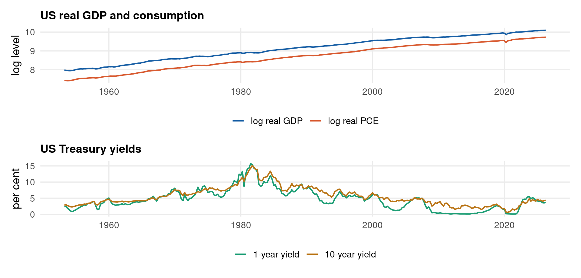
Code
import pandas as pd, matplotlib.pyplot as plt

fred = pd.read_csv("../data/ur-vecm-fred.csv", parse_dates=["date"])
fig, axes = plt.subplots(2, 1, figsize=(10, 4.8))
axes[0].plot(fred["date"], fred["lgdp"], color="#185FA5", lw=1.1,
             label="log real GDP")
axes[0].plot(fred["date"], fred["lpce"], color="#D85A30", lw=1.1,
             label="log real PCE")
axes[1].plot(fred["date"], fred["gs10"], color="#BA7517", lw=1.1,
             label="10-year yield")
axes[1].plot(fred["date"], fred["gs1"],  color="#1D9E75", lw=1.1,
             label="1-year yield")
axopts = axes[0].set(title="US real GDP and consumption", ylabel="log level")
axopts = axes[1].set(title="US Treasury yields", ylabel="per cent")
axes[0].text(0.02, 0.85, f"n = {len(fred)} quarters",
             transform=axes[0].transAxes, fontsize=11, color="#555555")
for ax in axes:
    ax.legend(fontsize=10)
plt.tight_layout()
plt.show()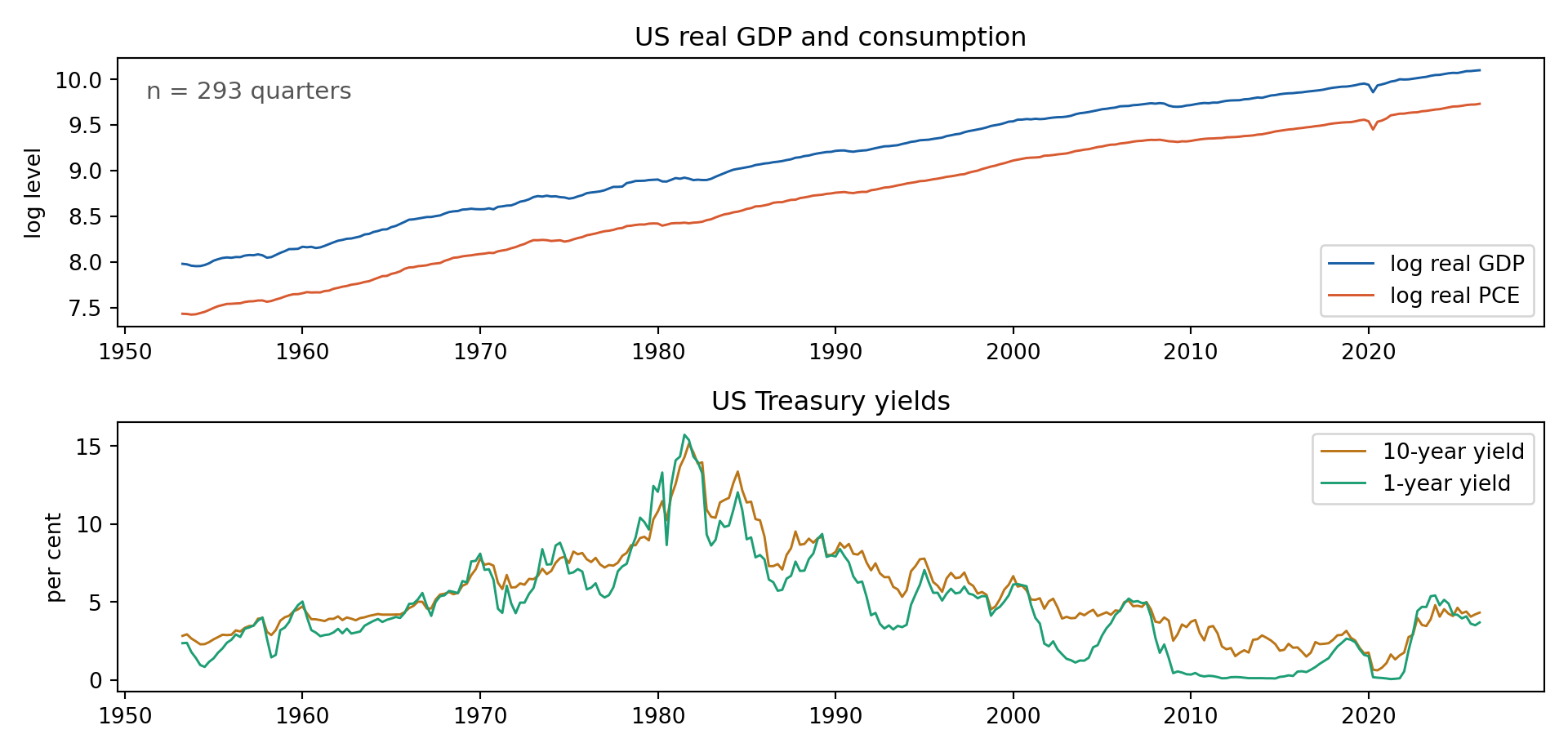
Code
    Variable |        Obs        Mean    Std. dev.       Min        Max
-------------+---------------------------------------------------------
        lgdp |        293     9.13165    .6318573   7.953386   10.09702
        lpce |        293    8.683982    .6765716   7.423239   9.730202
        gs10 |        293    5.523584    2.873639        .62      15.15
         gs1 |        293    4.615051    3.229879        .06      15.72


Time variable: qdate, 1953q2 to 2026q2
        Delta: 1 quarter
Four series, two pairs, two different reasons to expect a long-run relationship.
- log GDP and log consumption trend together over seventy years. The permanent income hypothesis says the ratio should be stationary — that is a cointegration restriction, and it is tested in Part V.
- The two Treasury yields wander over the same range without a common trend in levels, but the spread between them is what the expectations hypothesis restricts. They are the natural candidate for a cointegrating vector of \([1,-1]\).
Both pairs look non-stationary and neither looks like it is drifting apart permanently — which is exactly the configuration in which formal testing is needed, because the eye cannot separate “cointegrated” from “two independent walks that happen to move together”.
Why the CSV headers are lower case
The CSV stores its column names in lower case. Stata’s import delimited lower-cases variable names on the way in, so a header of GS10 would become gs10 there while R and Python kept GS10.
Writing lower case at source is what keeps the three tabs referring to the same variable.
Unit Root Results on FRED Data
Code
vars_to_test <- c("lgdp", "lpce", "gs10", "gs1")

results <- data.frame()
for (v in vars_to_test) {
  x   <- na.omit(fred_df[[v]])
  adf <- tseries::adf.test(x)
  pp  <- tseries::pp.test(x)
  kp  <- tseries::kpss.test(x, null = "Level")
  np  <- ng_perron(x, "trend")
  results <- rbind(results, data.frame(
    Variable = v,
    ADF   = round(adf$statistic, 3), ADF_p = round(adf$p.value, 3),
    PP    = round(pp$statistic, 3),
    KPSS  = round(kp$statistic, 3),
    MZt   = round(np["MZt"], 3)
  ))
}
print(results, row.names = FALSE)
Variable ADF ADF_p PP KPSS MZt Order
lgdp -1.293 0.874 -3.343 4.940 -0.703 I(1)
lpce -1.237 0.898 -3.035 4.951 -0.532 I(1)
gs10 -1.997 0.578 -6.965 1.370 -1.294 I(1)
gs1 -2.710 0.277 -12.118 1.374 -1.804 I(1)
KPSS 5% critical value 0.463 (reject stationarity above it)Ng-Perron MZt 5% critical value -2.91 (reject the unit root below it)Code
import pandas as pd, warnings
warnings.filterwarnings("ignore")
from statsmodels.tsa.stattools import adfuller, kpss
from arch.unitroot import PhillipsPerron

fred = pd.read_csv("../data/ur-vecm-fred.csv").dropna()
lines = [f"{'Variable':<10}{'ADF':>9}{'ADF p':>8}{'PP':>9}{'KPSS':>8}"]
for col in ["lgdp", "lpce", "gs10", "gs1"]:
    x  = fred[col].values
    a  = adfuller(x, autolag="AIC", regression="ct")
    pp = PhillipsPerron(x, trend="ct")
    kp = kpss(x, regression="c", nlags="auto")
    lines.append(f"{col:<10}{a[0]:>9.3f}{a[1]:>8.3f}"
                 f"{pp.stat:>9.3f}{kp[0]:>8.3f}")
lines.append("\nKPSS 5% critical value 0.463")
out = "\n".join(lines)
import sys; sys.stdout.write(out + "\n"); sys.stdout.flush()
Variable ADF ADF p PP KPSS
lgdp -0.971 0.948 -0.985 2.743
lpce -1.063 0.935 -1.081 2.750
gs10 -2.023 0.589 -1.906 0.774
gs1 -2.302 0.433 -2.304 0.799
KPSS 5% critical value 0.463
255Code
quietly import delimited "../data/ur-vecm-fred.csv", clear
quietly destring _all, replace
quietly gen date2 = date(date, "YMD")
quietly gen qdate = qofd(date2)
quietly format qdate %tq
quietly tsset qdate
foreach v in lgdp lpce gs10 gs1 {
    display ""
    display "=== `v' ==="
    quietly dfuller `v', trend lags(4)
    display "  ADF  = " %8.4f r(Zt)
    quietly pperron `v', trend lags(6)
    display "  PP   = " %8.4f r(Zt)
    kpss `v'
}
=== lgdp ===
ADF = -1.5517
PP = -1.1205
KPSS test for lgdp
Maxlag = 5 chosen by Schwert criterion
Autocovariances weighted by Bartlett kernel
Critical values for H0: lgdp is trend stationary
10%: 0.119 5% : 0.146 2.5%: 0.176 1% : 0.216
Lag order Test statistic
0 5.66
1 2.85
2 1.92
3 1.45
4 1.17
5 .983
=== lpce ===
ADF = -1.4395
PP = -1.1338
KPSS test for lpce
Maxlag = 5 chosen by Schwert criterion
Autocovariances weighted by Bartlett kernel
Critical values for H0: lpce is trend stationary
10%: 0.119 5% : 0.146 2.5%: 0.176 1% : 0.216
Lag order Test statistic
0 5.58
1 2.82
2 1.89
3 1.43
4 1.15
5 .968
=== gs10 ===
ADF = -2.2150
PP = -2.0139
KPSS test for gs10
Maxlag = 5 chosen by Schwert criterion
Autocovariances weighted by Bartlett kernel
Critical values for H0: gs10 is trend stationary
10%: 0.119 5% : 0.146 2.5%: 0.176 1% : 0.216
Lag order Test statistic
0 5.39
1 2.72
2 1.83
3 1.39
4 1.12
5 .94
=== gs1 ===
ADF = -3.0202
PP = -2.5613
KPSS test for gs1
Maxlag = 5 chosen by Schwert criterion
Autocovariances weighted by Bartlett kernel
Critical values for H0: gs1 is trend stationary
10%: 0.119 5% : 0.146 2.5%: 0.176 1% : 0.216
Lag order Test statistic
0 4.14
1 2.1
2 1.42
3 1.08
4 .877
5 .742All four series behave the same way, and the way we want: ADF and PP fail to reject the unit root, KPSS rejects stationarity, and the Ng-Perron \(MZ_t\) sits well above its critical value of \(-2.91\). Four tests with two different nulls all pointing the same direction is about as clean as macro data gets.
This is the confirmatory strategy of Part II doing its job. Had ADF failed to reject while KPSS also failed to reject, the honest conclusion would have been that the data cannot tell — not that the series is \(I(1)\).
Having established that all four are \(I(1)\), cointegration testing is now meaningful and Part V can proceed.
The Finland Money Demand System
The four-variable system used from here to the end of the deck, from Johansen (1988) and Johansen & Juselius (1990): Finnish money demand, 106 quarterly observations from 1958Q2 to 1984Q3.
| Variable | Meaning |
|---|---|
lrm1 |
log real money, M3 |
lny |
log real income |
lnmr |
log nominal interest rate |
difp |
change in the log price level, i.e. inflation |
Money demand theory predicts one long-run relation among the four:
\[ lrm_t = \eta\, lny_t - \theta\, lnmr_t - \phi\, difp_t + \text{stationary} \]
with \(\eta > 0\) from the transactions motive, and \(\theta, \phi > 0\) because both the interest rate and inflation are costs of holding money. One relation among four variables means \(r = 1\) and \(K - r = 3\) common stochastic trends — a testable prediction, not an assumption.
Code
fin_df <- read.csv("../data/ur-vecm-finland.csv")
fin_df <- fin_df |>
  mutate(date = seq(as.Date("1958-04-01"), by = "quarter", length.out = n()))

p1 <- ggplot(fin_df) + aes(date, lrm1) +
  geom_line(colour = "#185FA5", linewidth = 0.9) +
  labs(title = "log real money", x = NULL, y = NULL)
p2 <- ggplot(fin_df) + aes(date, lny) +
  geom_line(colour = "#1D9E75", linewidth = 0.9) +
  labs(title = "log real income", x = NULL, y = NULL)
p3 <- ggplot(fin_df) + aes(date, lnmr) +
  geom_line(colour = "#D85A30", linewidth = 0.9) +
  labs(title = "log nominal rate", x = NULL, y = NULL)
p4 <- ggplot(fin_df) + aes(date, difp) +
  geom_line(colour = "#BA7517", linewidth = 0.9) +
  labs(title = "inflation", x = NULL, y = NULL)

(p1 | p2) / (p3 | p4)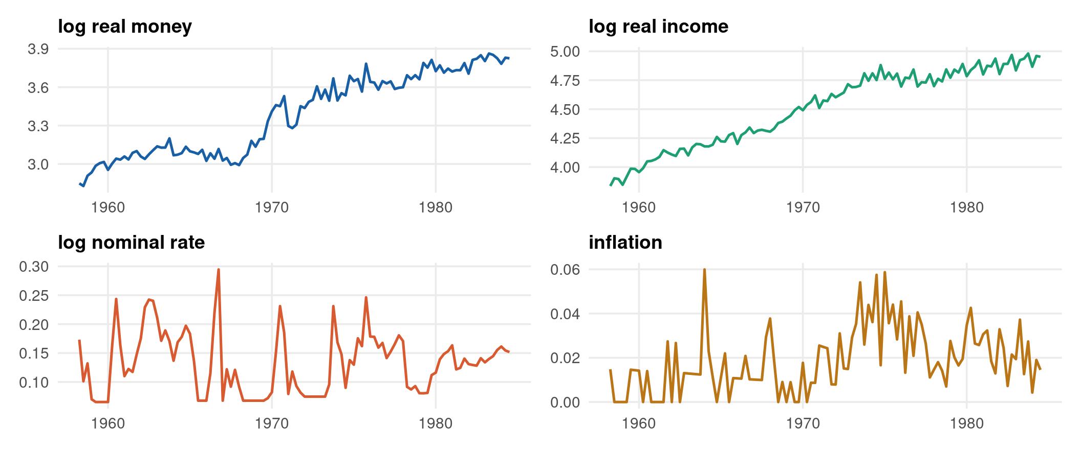
Code
import pandas as pd, matplotlib.pyplot as plt
import matplotlib.dates as mdates

fin = pd.read_csv("../data/ur-vecm-finland.csv")
fin.index = pd.date_range(start="1958-04-01", periods=len(fin), freq="QS")

cols   = ["lrm1", "lny", "lnmr", "difp"]
titles = ["log real money", "log real income", "log nominal rate", "inflation"]
colors = ["#185FA5", "#1D9E75", "#D85A30", "#BA7517"]

fig, axes = plt.subplots(2, 2, figsize=(11, 4.6))
for ax, col, title, color in zip(axes.flat, cols, titles, colors):
    ax.plot(fin.index, fin[col], color=color, lw=1.2)
    axopts = ax.set(title=title)
    ax.xaxis.set_major_formatter(mdates.DateFormatter("%Y"))
    ax.title.set_fontsize(12)
plt.suptitle(f"Finland money demand, {len(fin)} quarters 1958Q2-1984Q3",
             fontsize=13)
plt.tight_layout()
plt.show()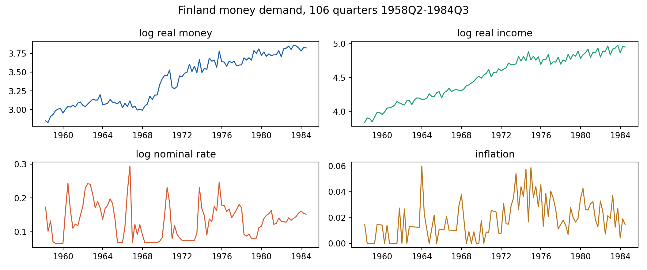
Code
    Variable |         N      Mean        SD       Min       p50       Max
-------------+------------------------------------------------------------
        lrm1 |  106.0000    3.3857    0.3151    2.8280    3.4515    3.8630
         lny |  106.0000    4.5105    0.3286    3.8365    4.5889    4.9807
        lnmr |  106.0000    0.1329    0.0519    0.0653    0.1330    0.2945
        difp |  106.0000    0.0187    0.0144    0.0000    0.0149    0.0599
--------------------------------------------------------------------------
The three log-level series each move across a wide range with no tendency to return — the visual signature of \(I(1)\). Inflation is different: it oscillates around a small positive mean, spikes with the 1970s oil shocks, and comes back. It is the one variable of the four that might be \(I(0)\).
That asymmetry has a practical consequence for the next slide. The three levels should be tested with a trend in the ADF specification; difp should not, because fitting a trend to a series that has none costs power for nothing.
Finland — Integration Orders
Code
ur_tbl <- data.frame()
for (v in c("lrm1", "lny", "lnmr", "difp")) {
  y_lev  <- fin_df[[v]]
  lev    <- urca::ur.df(y_lev,       type = "trend", selectlags = "AIC")
  dif    <- urca::ur.df(diff(y_lev), type = "drift", selectlags = "AIC")
  ur_tbl <- rbind(ur_tbl, data.frame(
    Variable  = v,
    ADF_level = round(lev@teststat[1], 3),
    cv5_level = lev@cval[1, "5pct"],
    ADF_diff  = round(dif@teststat[1], 3),
    cv5_diff  = dif@cval[1, "5pct"]
  ))
}
print(ur_tbl, row.names = FALSE)
Variable ADF_level cv5_level ADF_diff cv5_diff Order
lrm1 -2.340 -3.43 -7.242 -2.88 I(1)
lny -2.142 -3.43 -10.035 -2.88 I(1)
lnmr -4.732 -3.43 -8.225 -2.88 not I(1)
difp -4.200 -3.43 -9.991 -2.88 not I(1)Code
import pandas as pd, warnings
warnings.filterwarnings("ignore")
from statsmodels.tsa.stattools import adfuller, kpss

fin = pd.read_csv("../data/ur-vecm-finland.csv")
lines = [f"{'Variable':<10}{'ADF lev':>10}{'p':>8}{'ADF diff':>10}{'p':>8}{'order':>9}"]
for col in fin.columns:
    lev = adfuller(fin[col], maxlag=4, autolag="AIC", regression="ct")
    dif = adfuller(fin[col].diff().dropna(), maxlag=4, autolag="AIC",
                   regression="c")
    order = "I(1)" if lev[1] > 0.05 and dif[1] < 0.05 else "check"
    lines.append(f"{col:<10}{lev[0]:>10.3f}{lev[1]:>8.3f}"
                 f"{dif[0]:>10.3f}{dif[1]:>8.3f}{order:>9}")

lines.append("\nKPSS, H0 is stationarity:")
for col in fin.columns:
    stat, pval, *_ = kpss(fin[col], regression="c", nlags="auto")
    lines.append(f"  {col:<8} stat = {stat:.3f}  p = {pval:.3f}")

out = "\n".join(lines)
import sys; sys.stdout.write(out + "\n"); sys.stdout.flush()
Variable ADF lev p ADF diff p order
lrm1 -2.546 0.305 -5.040 0.000 I(1)
lny -1.565 0.806 -4.441 0.000 I(1)
lnmr -4.874 0.000 -7.208 0.000 check
difp -2.755 0.214 -10.297 0.000 I(1)
KPSS, H0 is stationarity:
lrm1 stat = 1.555 p = 0.010
lny stat = 1.579 p = 0.010
lnmr stat = 0.091 p = 0.100
difp stat = 0.783 p = 0.010
447Code
quietly import delimited "../data/ur-vecm-finland.csv", clear
quietly gen t = _n
quietly tsset t
foreach v in lrm1 lny lnmr difp {
    quietly dfuller `v', lags(2) trend
    local lev = r(Zt)
    quietly dfuller D.`v', lags(1)
    display "  `v'" _col(10) "ADF level = " %8.3f `lev' ///
        "   ADF difference = " %8.3f r(Zt)
}
display ""
display "5% critical values: trend -3.45, drift -2.89"
6. }
lrm1 ADF level = -2.874 ADF difference = -7.242
lny ADF level = -1.862 ADF difference = -10.035
lnmr ADF level = -4.696 ADF difference = -8.225
difp ADF level = -4.032 ADF difference = -9.991
5% critical values: trend -3.45, drift -2.89Each level fails to reject, each first difference rejects. That pair of results, in that order, is what licenses treating the system as \(I(1)\) and moving on to Johansen.
difp is the one to watch. It is already a first difference of a price level, so if it were \(I(1)\) the price level would be \(I(2)\) and the whole system would need re-specifying. The tests put it at \(I(1)\) on this sample at the 5% level, but it is the marginal case, and Johansen’s rank result should be checked for sensitivity to dropping it.
Pre-testing errors compound
Testing four variables at 5% each is four chances to be wrong. Unit root pre-testing feeds its errors forward into the rank test and then into the VECM.
That is a large part of why the ARDL bounds test, which needs no pre-testing, exists at all.
Johansen on the Finland System
Code
fin_df <- read.csv("../data/ur-vecm-finland.csv")

# K = 2 lags in LEVELS, so the VECM has one lag in differences
jo_trace <- urca::ca.jo(fin_df[, c("lrm1", "lny", "lnmr", "difp")],
                        type = "trace", ecdet = "none", K = 2,
                        spec = "longrun")
summary(jo_trace)

# The cointegrating vector, normalised on lrm1
cajorls(jo_trace, r = 1)$beta
Hypothesis Trace Trace_5pct MaxEigen MaxE_5pct
r = 0 | 79.209 48.28 39.942 27.14
r <= 1 | 39.267 31.52 29.230 21.07
r <= 2 | 10.037 17.95 7.787 14.90
r <= 3 | 2.251 8.18 2.251 8.18
Cointegrating vector, normalised on lrm1: ect1
lrm1.l2 1.0000
lny.l2 -1.1172
lnmr.l2 -4.6829
difp.l2 5.4674
Loading coefficients alpha: lrm1.d lny.d lnmr.d difp.d
0.0569 0.0628 0.1066 -0.0029 Code
import numpy as np, pandas as pd, warnings
warnings.filterwarnings("ignore")
from statsmodels.tsa.vector_ar.vecm import VECM, select_coint_rank

fin = pd.read_csv("../data/ur-vecm-finland.csv")

sel = select_coint_rank(fin, det_order=0, k_ar_diff=1, method="trace",
                        signif=0.05)
# Impose r = 1, the rank selected by the R and Stata trace tests. See the
# reading note: statsmodels applies a different deterministic convention and
# selects a higher rank on the same data.
res = VECM(fin, k_ar_diff=1, coint_rank=1, deterministic="co").fit()

lines = [f"statsmodels trace test selects r = {sel.rank}",
         "imposing r = 1 to match the R and Stata specification",
         "",
         "Cointegrating vector beta, normalised on lrm1:",
         "  " + "  ".join(f"{v:>9.4f}" for v in res.beta.ravel()),
         "",
         "Loading coefficients alpha:",
         "  " + "  ".join(f"{v:>9.4f}" for v in res.alpha.ravel())]
out = "\n".join(lines)
import sys; sys.stdout.write(out + "\n"); sys.stdout.flush()
statsmodels trace test selects r = 2
imposing r = 1 to match the R and Stata specification
Cointegrating vector beta, normalised on lrm1:
1.0000 -1.1172 -4.6829 5.4674
Loading coefficients alpha:
0.0569 0.0628 0.1066 -0.0029
258Code
quietly import delimited "../data/ur-vecm-finland.csv", clear
quietly gen t = _n
quietly tsset t
vecrank lrm1 lny lnmr difp, trend(constant) lags(2) max
quietly vec lrm1 lny lnmr difp, trend(constant) lags(2) rank(1)
display ""
display "Cointegrating vector, normalised on lrm1:"
matrix b = e(beta)
matrix list b
Johansen tests for cointegration
Trend: Constant Number of obs = 104
Sample: 3 thru 106 Number of lags = 2
--------------------------------------------------------------
Critical
Maximum Trace value
rank Params LL Eigenvalue statistic 5%
0 20 835.368 . 79.2089 47.21
1 27 855.33892 0.31891 39.2671 29.68
2 32 869.95374 0.24501 10.0374* 15.41
3 35 873.84718 0.07214 2.2506 3.76
4 36 874.97246 0.02141
--------------------------------------------------------------
Critical
Maximum ------Eigenvalue----- value
rank Params LL Maximum 5%
0 20 835.368 . 39.9418 27.07
1 27 855.33892 0.31891 29.2297 20.97
2 32 869.95374 0.24501 7.7869 14.07
3 35 873.84718 0.07214 2.2506 3.76
4 36 874.97246 0.02141
--------------------------------------------------------------
* selected rank
Cointegrating vector, normalised on lrm1:
b[1,5]
_ce1: _ce1: _ce1: _ce1: _ce1:
lrm1 lny lnmr difp _cons
beta 1 -1.1171632 -4.6829151 5.4674369 2.2918446The trace sequence rejects \(r = 0\) decisively and then fails to reject \(r \le 1\), so \(\hat r = 1\): one long-run relationship among the four variables and three common stochastic trends. That is what money demand theory predicts, and it is not something the estimation was told to find.
The normalised vector is the same in all three languages to four decimals:
\[ ECT_t = lrm1_t - 1.1172\,lny_t - 4.6829\,lnmr_t + 5.4674\,difp_t \]
An income elasticity near 1.1 is plausible for money demand. The interest-rate and inflation coefficients carry the signs the theory expects once the normalisation convention is unwound.
When statsmodels picks a different rank
statsmodels selects a higher rank on this data — 2 or 3 depending on det_order. This is not a bug in either package.
The Johansen critical values depend on which deterministic terms are restricted to the cointegrating space, and the three programs do not share a default.
Fix the specification explicitly, in every language, and report it. The estimates conditional on \(r = 1\) then agree exactly.
Part V — Error Correction and the VECM
δεῖ γὰρ πρὸς οἴκους νοστίμου σωτηρίας
κάμψαι διαύλου θάτερον κῶλον πάλιν·
they must still round the far leg of the double course, and come safe home
Αἰσχύλος, Ἀγαμέμνων 343–344
The Error Correction Model
If \(y_t\) and \(x_t\) are \(I(1)\) and \(y_t - \beta x_t \sim I(0)\), the Granger representation theorem guarantees that at least one of the two adjusts:
\[ \Delta y_t = \alpha_y(y_{t-1} - \beta x_{t-1}) + \text{short-run terms} + \varepsilon_{yt} \]
\[ \Delta x_t = \alpha_x(y_{t-1} - \beta x_{t-1}) + \text{short-run terms} + \varepsilon_{xt} \]
with \(\alpha_y \ne 0\) or \(\alpha_x \ne 0\). The bracketed term is the error correction term: last period’s deviation from long-run equilibrium.
Two-step estimation. Take \(\hat u_{t-1} = y_{t-1} - \hat\beta x_{t-1}\) from the Engle-Granger first stage, then run
\[ \Delta y_t = c + \alpha\hat u_{t-1} + \sum_{j=1}^{p}\gamma_j\Delta y_{t-j} + \sum_{j=0}^{q}\delta_j\Delta x_{t-j} + \varepsilon_t \]
The sign is the whole diagnostic. \(\alpha\) must be negative — a positive deviation from equilibrium has to pull \(\Delta y\) down, or the system is explosive rather than error-correcting.
\(\lvert\alpha\rvert\) is the fraction of a disequilibrium removed each period, which converts directly into a half-life:
\[ \tau_{1/2} = \frac{\log(0.5)}{\log(1+\hat\alpha)} \]
| \(\hat\alpha\) | Half-life | Reading |
|---|---|---|
| \(-0.05\) | ~13 quarters | Very slow, over three years |
| \(-0.13\) | ~5 quarters | Typical monetary transmission |
| \(-0.50\) | ~1 quarter | Fast |
| \(-1.00\) | Immediate | Full correction within the period |
Where the usual t-distribution is legitimate
Because \(\hat u_{t-1}\) is stationary, the \(t\)-statistic on \(\alpha\) has its usual distribution — the non-standard asymptotics live entirely in the first step.
This is one of the few places in this deck where a conventional \(t\)-test is legitimate.
ECM — Code
Code
sim_df <- read.csv("../data/ur-vecm-sim.csv")

# Step 1: the long-run relation
lr_fit  <- lm(y_c ~ x_c, data = sim_df)
ect_hat <- residuals(lr_fit)

# Step 2: the short-run equation, with last period's disequilibrium in it
ecm_df <- data.frame(
  dy      = diff(sim_df$y_c),
  dx      = diff(sim_df$x_c),
  ect_lag = ect_hat[-length(ect_hat)]
)
ecm_df <- ecm_df |> mutate(dy_lag = c(NA, dy[-length(dy)]))
ecm_fit <- lm(dy ~ ect_lag + dy_lag + dx, data = na.omit(ecm_df))
summary(ecm_fit)
Estimate Std. Error t value Pr(>|t|)
(Intercept) 0.0006 0.0298 0.0205 0.9837
ect_lag -0.5881 0.0537 -10.9451 0.0000
dy_lag 0.0063 0.0147 0.4275 0.6693
dx 2.0014 0.0307 65.2962 0.0000
Speed of adjustment alpha = -0.5881Half-life = 0.78 periodsThe DGP set the AR(1) coefficient of the equilibrium error to 0.4,so the implied alpha is 0.4 - 1 = -0.6.Code
import numpy as np, pandas as pd
import statsmodels.api as sm

sim = pd.read_csv("../data/ur-vecm-sim.csv")
lr  = sm.OLS(sim["y_c"], sm.add_constant(sim["x_c"])).fit()
ect = lr.resid

d = pd.DataFrame({
    "dy":      sim["y_c"].diff(),
    "dx":      sim["x_c"].diff(),
    "ect_lag": ect.shift(1),
}).dropna()
d["dy_lag"] = d["dy"].shift(1)
d = d.dropna()

ecm = sm.OLS(d["dy"], sm.add_constant(d[["ect_lag", "dy_lag", "dx"]])).fit()
a_hat = ecm.params["ect_lag"]

lines = [str(ecm.summary().tables[1]),
         f"\nSpeed of adjustment alpha = {a_hat:.4f}",
         f"Half-life = {np.log(0.5)/np.log(1+a_hat):.2f} periods",
         "The DGP implies alpha = 0.4 - 1 = -0.6."]
out = "\n".join(lines)
import sys; sys.stdout.write(out + "\n"); sys.stdout.flush()
==============================================================================
coef std err t P>|t| [0.025 0.975]
------------------------------------------------------------------------------
const 0.0006 0.030 0.020 0.984 -0.058 0.059
ect_lag -0.5881 0.054 -10.945 0.000 -0.694 -0.482
dy_lag 0.0063 0.015 0.428 0.669 -0.023 0.035
dx 2.0014 0.031 65.296 0.000 1.941 2.062
==============================================================================
Speed of adjustment alpha = -0.5881
Half-life = 0.78 periods
The DGP implies alpha = 0.4 - 1 = -0.6.
734Code
quietly import delimited "../data/ur-vecm-sim.csv", clear
quietly destring _all, replace
quietly tsset t
quietly regress y_c x_c
quietly predict ect_hat, residuals
quietly gen dy_c = D.y_c
quietly gen dx_c = D.x_c
quietly gen ect_l = L.ect_hat
regress dy_c ect_l L.dy_c dx_c
display ""
display "Speed of adjustment alpha = " %8.4f _b[ect_l]
display "Half-life = " %6.2f ln(0.5)/ln(1+_b[ect_l]) " periods"
Source | SS df MS Number of obs = 298
-------------+---------------------------------- F(3, 294) = 1484.85
Model | 1175.27731 3 391.759103 Prob > F = 0.0000
Residual | 77.568062 294 .263836946 R-squared = 0.9381
-------------+---------------------------------- Adj R-squared = 0.9375
Total | 1252.84537 297 4.21833458 Root MSE = .51365
------------------------------------------------------------------------------
dy_c | Coefficient Std. err. t P>|t| [95% conf. interval]
-------------+----------------------------------------------------------------
ect_l | -.588072 .0537295 -10.95 0.000 -.6938151 -.4823288
|
dy_c |
L1. | .0062736 .0146734 0.43 0.669 -.0226046 .0351518
|
dx_c | 2.001444 .0306518 65.30 0.000 1.941119 2.061769
_cons | .0006108 .0298054 0.02 0.984 -.0580483 .0592698
------------------------------------------------------------------------------
Speed of adjustment alpha = -0.5881
Half-life = 0.78 periodsThe known truth is available here too. The DGP made the equilibrium error an AR(1) with coefficient 0.4, so \(u_t - u_{t-1} = -0.6\,u_{t-1} + \eta_t\) and the correct \(\alpha\) is \(-0.6\). The estimate lands close to it in all three languages, with a half-life of roughly one period.
Notice what the ECM has bought. The dependent variable is a difference, so it is \(I(0)\) and standard inference applies — but the equation still contains the long-run relationship, in levels, through \(\hat u_{t-1}\). Nothing has been thrown away by differencing, which is exactly what a plain VAR in differences would have done.
DOLS and the Long-Run Elasticity
The Engle-Granger first stage estimates \(\beta\) consistently, and even superconsistently — but its standard error is wrong, so a confidence interval built from it has no coverage guarantee. The culprit is the correlation between \(\Delta x_t\) and \(u_t\) that cointegration itself induces.
Stock & Watson (1993) fix it by adding leads and lags of \(\Delta x\) to the static regression:
\[ y_t = \alpha + \beta x_t + \sum_{j=-q}^{q}\delta_j\Delta x_{t-j} + \varepsilon_t \]
The augmentation absorbs the endogeneity and the serial correlation. What is left is asymptotically normal:
\[ \hat\beta_{\text{DOLS}} \sim N(\beta, V) \quad\Longrightarrow\quad \text{valid } t\text{-tests and confidence intervals} \]
A rule of thumb for \(q\): 1 or 2 for quarterly data, more when \(T > 200\).
Report the DOLS estimate with its standard error, and use OLS only to generate residuals for the second step.
If DOLS and OLS differ substantially, that difference is itself information: the endogeneity the leads and lags are correcting for is large in this sample.
FMOLS, the other standard fix
Fully modified OLS (Phillips-Hansen) is the other standard fix and targets the same problem non-parametrically.
DOLS is easier to explain and to implement identically in three languages, which is why it is the one shown here.
DOLS — Code
Code
fin_df <- read.csv("../data/ur-vecm-finland.csv")

q       <- 2
dlny    <- c(NA, diff(fin_df$lny))
dols_df <- fin_df[, c("lrm1", "lny")]
for (k in -q:q) {
  dols_df[[paste0("dlny_", k)]] <-
    if (k < 0) dplyr::lead(dlny, n = -k) else dplyr::lag(dlny, n = k)
}
dols_fit <- lm(lrm1 ~ ., data = na.omit(dols_df))

ols_fit <- lm(lrm1 ~ lny, data = fin_df)
cat(sprintf("OLS  beta = %.4f  (SE %.4f, not valid)\n",
            coef(ols_fit)["lny"], sqrt(diag(vcov(ols_fit)))["lny"]))
cat(sprintf("DOLS beta = %.4f  (SE %.4f, valid)\n",
            coef(dols_fit)["lny"], sqrt(diag(vcov(dols_fit)))["lny"]))
Estimator Beta SE SE_valid
OLS (static) 0.9206 0.0263 no
DOLS (2 leads, 2 lags) 0.9289 0.0315 yes
DOLS 95% CI for the long-run income elasticity: [0.8670, 0.9907]Code
import pandas as pd
import statsmodels.api as sm

fin = pd.read_csv("../data/ur-vecm-finland.csv")
q   = 2
d   = fin[["lrm1", "lny"]].copy()
d["dlny"] = d["lny"].diff()
for k in range(-q, q + 1):
    d[f"dlny_{k}"] = d["dlny"].shift(k)
d = d.drop(columns="dlny").dropna()

X_d  = sm.add_constant(d.drop(columns="lrm1"))
dols = sm.OLS(d["lrm1"], X_d).fit()
ols  = sm.OLS(fin["lrm1"], sm.add_constant(fin["lny"])).fit()

lines = [f"{'Estimator':<26}{'beta':>10}{'SE':>10}{'valid SE':>10}",
         f"{'OLS (static)':<26}{ols.params['lny']:>10.4f}"
         f"{ols.bse['lny']:>10.4f}{'no':>10}",
         f"{'DOLS (2 leads, 2 lags)':<26}{dols.params['lny']:>10.4f}"
         f"{dols.bse['lny']:>10.4f}{'yes':>10}",
         f"\nDOLS 95% CI: [{dols.params['lny'] - 1.96*dols.bse['lny']:.4f}, "
         f"{dols.params['lny'] + 1.96*dols.bse['lny']:.4f}]"]
out = "\n".join(lines)
import sys; sys.stdout.write(out + "\n"); sys.stdout.flush()
Estimator beta SE valid SE
OLS (static) 0.9206 0.0263 no
DOLS (2 leads, 2 lags) 0.9289 0.0315 yes
DOLS 95% CI: [0.8670, 0.9907]
202Code
quietly import delimited "../data/ur-vecm-finland.csv", clear
quietly gen t = _n
quietly tsset t
quietly regress lrm1 lny
display "OLS  beta = " %8.4f _b[lny] "   SE = " %8.4f _se[lny] "  (not valid)"
quietly gen d_lny = D.lny
forvalues k = 1/2 {
    quietly gen d_lny_l`k' = L`k'.d_lny
    quietly gen d_lny_f`k' = F`k'.d_lny
}
regress lrm1 lny d_lny d_lny_l1 d_lny_l2 d_lny_f1 d_lny_f2
display ""
display "DOLS beta = " %8.4f _b[lny] "   SE = " %8.4f _se[lny] "  (valid)"
OLS beta = 0.9206 SE = 0.0263 (not valid)
Source | SS df MS Number of obs = 101
-------------+---------------------------------- F(6, 94) = 170.41
Model | 8.42496009 6 1.40416002 Prob > F = 0.0000
Residual | .774536357 94 .008239748 R-squared = 0.9158
-------------+---------------------------------- Adj R-squared = 0.9104
Total | 9.19949645 100 .091994965 Root MSE = .09077
------------------------------------------------------------------------------
lrm1 | Coefficient Std. err. t P>|t| [95% conf. interval]
-------------+----------------------------------------------------------------
lny | .9288699 .0315439 29.45 0.000 .8662387 .9915011
d_lny | -.2851877 .2834156 -1.01 0.317 -.8479161 .2775407
d_lny_l1 | -.1808101 .2873737 -0.63 0.531 -.7513972 .3897771
d_lny_l2 | .0915267 .3017611 0.30 0.762 -.5076271 .6906805
d_lny_f1 | -.0093134 .2934317 -0.03 0.975 -.5919288 .5733021
d_lny_f2 | -.0184775 .3038253 -0.06 0.952 -.6217299 .5847748
_cons | -.8023728 .1471343 -5.45 0.000 -1.094511 -.5102343
------------------------------------------------------------------------------
DOLS beta = 0.9289 SE = 0.0315 (valid)The two estimates of the long-run income elasticity of money demand sit close to each other, which is reassuring: on this sample the endogeneity correction does not move the point estimate much. The standard errors are what change, and only the DOLS one supports a confidence interval.
The elasticity above unity is the standard finding for this dataset. Money holdings rise slightly more than proportionally with real income over the long run.
DOLS and Johansen answer different questions
The bivariate DOLS here and the four-variable Johansen system on the next slides answer different questions. DOLS estimates one long-run coefficient having assumed a single relation exists; Johansen estimates how many relations there are and what they look like, jointly.
Where both are valid they should broadly agree — and here the income coefficient from the four-variable system, 1.1172, is in the same territory.
From Johansen to the VECM
With the rank \(r\) selected, estimate the full system:
\[ \Delta\mathbf{y}_t = \boldsymbol\alpha\boldsymbol\beta'\mathbf{y}_{t-1} + \boldsymbol\Gamma_1\Delta\mathbf{y}_{t-1} + \cdots + \boldsymbol\Gamma_{p-1}\Delta\mathbf{y}_{t-p+1} + \boldsymbol\mu + \mathbf{u}_t \]
Everything on the right is stationary: \(\Delta\mathbf{y}\) by construction, and \(\boldsymbol\beta'\mathbf{y}_{t-1}\) because that is what cointegration means. This is why the VECM has conventional inference where the levels VAR does not.
Three routes in R, and they are not interchangeable:
| Route | Gives | Use when |
|---|---|---|
urca::cajorls(jo, r) |
Restricted system as lm objects |
You want coeftest or robust standard errors |
tsDyn::VECM(data, lag, r) |
Standalone ML or two-step OLS fit | You will extend to TVECM |
vars::vec2var(jo, r) |
A varest object |
You need IRF, FEVD or diagnostics |
With \(r = 1\) and \(K = 4\), \(\boldsymbol\alpha\) is a single column and each element says how that equation responds to last period’s disequilibrium:
\[ \begin{pmatrix}\Delta lrm1_t \\ \Delta lny_t \\ \Delta lnmr_t \\ \Delta difp_t\end{pmatrix} = \begin{pmatrix}\alpha_1 \\ \alpha_2 \\ \alpha_3 \\ \alpha_4\end{pmatrix} ECT_{t-1} + \cdots \]
- \(\alpha_i \ne 0\) — variable \(i\) responds to the disequilibrium and helps restore it
- \(\alpha_i = 0\) — variable \(i\) is weakly exogenous for the long-run parameters; it pushes the system but is not pushed by it
Which elements are zero is an economic claim, and it is testable. Money demand theory says income should be weakly exogenous: the money market does not drive national income. That test is two slides ahead.
K counts levels, lag counts differences
ca.jo(K = 2) and VECM(lag = 1) describe the same model. \(K\) counts lags in levels, lag counts lags in differences, and they differ by one.
Getting this wrong changes the estimates without producing any error.
VECM — Estimation
Code
fin_df <- read.csv("../data/ur-vecm-finland.csv")
Yf <- fin_df[, c("lrm1", "lny", "lnmr", "difp")]

jo_trace <- urca::ca.jo(Yf, type = "trace", ecdet = "none", K = 2,
                        spec = "longrun")

# Route 1: restricted least squares from the Johansen fit
vecm_ur <- urca::cajorls(jo_trace, r = 1)
vecm_ur$beta
vecm_ur$rlm$coefficients["ect1", ]

# Route 2: tsDyn, note lag = K - 1
vecm_ts <- tsDyn::VECM(Yf, lag = 1, r = 1, estim = "ML", include = "const")
summary(vecm_ts)
Cointegrating vector beta, normalised on lrm1: ect1
lrm1.l2 1.0000
lny.l2 -1.1172
lnmr.l2 -4.6829
difp.l2 5.4674
Loading coefficients: Equation Alpha HalfLife
lrm1.d 0.0569 NA
lny.d 0.0628 NA
lnmr.d 0.1066 NA
difp.d -0.0029 238.67
tsDyn::VECM(lag = 1) reproduces the same system from ca.jo(K = 2).Log-likelihood: 855.339Code
import numpy as np, pandas as pd, warnings
warnings.filterwarnings("ignore")
from statsmodels.tsa.vector_ar.vecm import VECM

fin = pd.read_csv("../data/ur-vecm-finland.csv")
res = VECM(fin, k_ar_diff=1, coint_rank=1, deterministic="co").fit()

lines = ["Cointegrating vector beta, normalised on lrm1:",
         "  " + "  ".join(f"{c}={v:.4f}"
                          for c, v in zip(fin.columns, res.beta.ravel())),
         "",
         f"{'Equation':<10}{'alpha':>10}{'half-life':>12}"]
for c, a in zip(fin.columns, res.alpha.ravel()):
    hl = f"{np.log(0.5)/np.log(1+a):.2f}" if -1 < a < 0 else "-"
    lines.append(f"{c:<10}{a:>10.4f}{hl:>12}")

out = "\n".join(lines)
import sys; sys.stdout.write(out + "\n"); sys.stdout.flush()
Cointegrating vector beta, normalised on lrm1:
lrm1=1.0000 lny=-1.1172 lnmr=-4.6829 difp=5.4674
Equation alpha half-life
lrm1 0.0569 -
lny 0.0628 -
lnmr 0.1066 -
difp -0.0029 242.44
267Code
Vector error-correction model

Sample: 3 thru 106                              Number of obs     =        104
                                                AIC               =  -15.92959
Log likelihood =  855.3389                      HQIC              =  -15.65146
Det(Sigma_ml)  =  8.44e-13                      SBIC              =  -15.24307

Equation           Parms      RMSE     R-sq      chi2     P>chi2
----------------------------------------------------------------
D_lrm1                6     .060709   0.2936   40.72793   0.0000
D_lny                 6     .046012   0.4668   85.79417   0.0000
D_lnmr                6      .03626   0.3754   58.90069   0.0000
D_difp                6      .01309   0.3583   54.72582   0.0000
----------------------------------------------------------------

------------------------------------------------------------------------------
             | Coefficient  Std. err.      z    P>|z|     [95% conf. interval]
-------------+----------------------------------------------------------------
D_lrm1       |
        _ce1 |
         L1. |   .0569323   .0279996     2.03   0.042      .002054    .1118106
             |
        lrm1 |
         LD. |  -.4328314   .1164121    -3.72   0.000     -.660995   -.2046678
             |
         lny |
         LD. |  -.1744005    .130555    -1.34   0.182    -.4302837    .0814827
             |
        lnmr |
         LD. |   .1654493   .1585809     1.04   0.297    -.1453635    .4762621
             |
        difp |
         LD. |  -.3580337   .4299486    -0.83   0.405    -1.200717      .48465
             |
       _cons |   .0087753   .0069165     1.27   0.205    -.0047808    .0223313
-------------+----------------------------------------------------------------
D_lny        |
        _ce1 |
         L1. |   .0627769   .0212212     2.96   0.003     .0211842    .1043697
             |
        lrm1 |
         LD. |   -.249962   .0882298    -2.83   0.005    -.4228893   -.0770348
             |
         lny |
         LD. |  -.4693646   .0989489    -4.74   0.000    -.6633008   -.2754284
             |
        lnmr |
         LD. |   .1867029   .1201899     1.55   0.120    -.0488649    .4222707
             |
        difp |
         LD. |  -.5051479   .3258619    -1.55   0.121    -1.143826    .1335297
             |
       _cons |   .0100427   .0052421     1.92   0.055    -.0002316    .0203169
-------------+----------------------------------------------------------------
D_lnmr       |
        _ce1 |
         L1. |   .1065943   .0167236     6.37   0.000     .0738165     .139372
             |
        lrm1 |
         LD. |   -.321085   .0695307    -4.62   0.000    -.4573628   -.1848073
             |
         lny |
         LD. |    .128211    .077978     1.64   0.100    -.0246231    .2810451
             |
        lnmr |
         LD. |   .2698705   .0947173     2.85   0.004     .0842281     .455513
             |
        difp |
         LD. |  -.2909226      .2568    -1.13   0.257    -.7942413    .2123961
             |
       _cons |  -.0105928   .0041311    -2.56   0.010    -.0186895    -.002496
-------------+----------------------------------------------------------------
D_difp       |
        _ce1 |
         L1. |   -.002855   .0060373    -0.47   0.636    -.0146878    .0089779
             |
        lrm1 |
         LD. |   .0446026   .0251007     1.78   0.076    -.0045938     .093799
             |
         lny |
         LD. |  -.0220766   .0281502    -0.78   0.433    -.0772499    .0330967
             |
        lnmr |
         LD. |  -.0056451   .0341931    -0.17   0.869    -.0726623     .061372
             |
        difp |
         LD. |  -.5293738   .0927051    -5.71   0.000    -.7110725   -.3476752
             |
       _cons |   .0003199   .0014913     0.21   0.830     -.002603    .0032429
------------------------------------------------------------------------------

Cointegrating equations

Equation           Parms    chi2     P>chi2
-------------------------------------------
_ce1                  3   148.5084   0.0000
-------------------------------------------

Identification:  beta is exactly identified

                 Johansen normalization restriction imposed
------------------------------------------------------------------------------
        beta | Coefficient  Std. err.      z    P>|z|     [95% conf. interval]
-------------+----------------------------------------------------------------
_ce1         |
        lrm1 |          1          .        .       .            .           .
         lny |  -1.117163    .121917    -9.16   0.000    -1.356116   -.8782102
        lnmr |  -4.682915   .6854063    -6.83   0.000    -6.026287   -3.339543
        difp |   5.467437    3.31626     1.65   0.099    -1.032313    11.96719
       _cons |   2.291845          .        .       .            .           .
------------------------------------------------------------------------------
The three languages return the same cointegrating vector and the same loadings to four decimals:
\[ \boldsymbol\beta' = (1,\; -1.1172,\; -4.6829,\; 5.4674), \qquad \boldsymbol\alpha' = (0.0569,\; 0.0628,\; 0.1066,\; -0.0029) \]
That agreement is worth pausing on, because nothing else in this deck matches this cleanly. The Johansen procedure is a solved eigenvalue problem with no tuning parameters once the rank, lag order and deterministic specification are fixed — so once those three are pinned down, the three implementations have nothing left to disagree about.
The last loading, on inflation, is essentially zero. That is the first hint of weak exogeneity, and the next slide tests it properly.
estat cointegration does not exist
estat cointegration is not a Stata command and never was; the cointegrating vector is already in the vec output and in e(beta).
Reaching for a postestimation command that does not exist is a good way to lose a whole chunk’s output, because Stata errors print as ordinary text rather than as a failed cell.
VECM — Diagnostics and Stability
| Check | Test | R |
|---|---|---|
| No residual serial correlation | Portmanteau / LM | vars::serial.test() |
| Normal residuals | Multivariate Jarque-Bera | vars::normality.test() |
| No ARCH | Multivariate ARCH-LM | vars::arch.test() |
| Stability | Companion matrix moduli | vars::roots() |
The roots check is the one with a twist. A cointegrated system of rank \(r\) has exactly \(K - r\) unit roots by construction — they are the common stochastic trends. Seeing moduli equal to 1 is correct here; what would signal a problem is a modulus above 1, or more unit roots than \(K - r\).
Portmanteau test for serial correlation: stat = 392.424, p = 0.0000Multivariate ARCH-LM: stat = 506.333, p = 0.4127
Companion matrix moduli: 1, 1, 1, 0.5999, 0.5999, 0.4698, 0.4698, 0.2254Unit roots expected for K - r = 3; largest non-unit modulus = 0.5999Code
import numpy as np, pandas as pd, warnings
warnings.filterwarnings("ignore")
from statsmodels.tsa.vector_ar.vecm import VECM
from statsmodels.stats.stattools import jarque_bera

fin = pd.read_csv("../data/ur-vecm-finland.csv")
res = VECM(fin, k_ar_diff=1, coint_rank=1, deterministic="co").fit()

resid = res.resid
lines = ["Residual diagnostics, equation by equation:",
         f"{'Equation':<10}{'JB stat':>10}{'JB p':>9}{'AC(1)':>9}"]
for j, c in enumerate(fin.columns):
    e  = resid[:, j]
    jb = jarque_bera(e)
    ac = np.corrcoef(e[1:], e[:-1])[0, 1]
    lines.append(f"{c:<10}{jb[0]:>10.3f}{jb[1]:>9.4f}{ac:>9.4f}")

# Companion matrix of the VAR representation
A    = res.var_rep
K, p = A.shape[1], A.shape[0]
comp = np.zeros((K * p, K * p))
comp[:K, :] = np.hstack([A[i] for i in range(p)])
if p > 1:
    comp[K:, :K * (p - 1)] = np.eye(K * (p - 1))
mods = np.sort(np.abs(np.linalg.eigvals(comp)))[::-1]
lines.append("\nCompanion matrix moduli: " +
             ", ".join(f"{m:.4f}" for m in mods))
lines.append(f"Largest non-unit modulus: {mods[mods < 0.9995].max():.4f}")

out = "\n".join(lines)
import sys; sys.stdout.write(out + "\n"); sys.stdout.flush()
Residual diagnostics, equation by equation:
Equation JB stat JB p AC(1)
lrm1 1.687 0.4303 0.0590
lny 5.866 0.0532 -0.0333
lnmr 17.429 0.0002 0.0219
difp 2.446 0.2943 -0.0455
Companion matrix moduli: 1.0000, 1.0000, 1.0000, 0.5999, 0.5999, 0.4698, 0.4698, 0.2254
Largest non-unit modulus: 0.5999
361Code
   Lagrange-multiplier test
  +--------------------------------------+
  | lag  |      chi2    df   Prob > chi2 |
  |------+-------------------------------|
  |   1  |   21.4157    16     0.16308   |
  |   2  |   57.0521    16     0.00000   |
  |   3  |   26.2213    16     0.05099   |
  |   4  |   53.9942    16     0.00001   |
  +--------------------------------------+
   H0: no autocorrelation at lag order


   Eigenvalue stability condition
  +----------------------------------------+
  |        Eigenvalue        |   Modulus   |
  |--------------------------+-------------|
  |          1               |         1   |
  |          1               |         1   |
  |          1               |         1   |
  |  -.5990289 + .03256747i  |   .599914   |
  |  -.5990289 - .03256747i  |   .599914   |
  |   .3668692 +   .293499i  |   .469824   |
  |   .3668692 -   .293499i  |   .469824   |
  |  -.2253609               |   .225361   |
  +----------------------------------------+
   The VECM specification imposes 3 unit moduli.
Read vecstable and vars::roots() the same way. With \(K = 4\) and \(r = 1\) there should be exactly three moduli equal to 1 — the three common stochastic trends the rank test already told us about — and everything else strictly inside the unit circle. That is what all three tabs report, so the rank selection and the stability check corroborate each other.
The serial correlation and ARCH tests are about whether the lag order is adequate. A rejection there usually means adding a lag rather than abandoning the specification.
Which diagnostic failure actually matters
Non-normal residuals are common in macro data and are not fatal: the Johansen estimator remains consistent, and the asymptotic distribution of the rank statistics does not depend on normality.
Serial correlation is the serious one, because it means the model is misspecified.
Weak Exogeneity and Restrictions on β
Both are linear restrictions with likelihood ratio tests, and both are answering economic questions rather than statistical ones.
Weak exogeneity — a restriction on \(\boldsymbol\alpha\). Variable \(i\) is weakly exogenous for the long-run parameters if it does not respond to the disequilibrium:
\[ H_0: \alpha_i = 0 \]
Written as \(\boldsymbol\alpha = \mathbf{A}\boldsymbol\psi\) for a known \(K\times(K-1)\) matrix \(\mathbf{A}\) that deletes row \(i\). Under \(H_0\) the statistic is \(\chi^2(r)\).
Structural restrictions — a restriction on \(\boldsymbol\beta\). Write \(\boldsymbol\beta = \mathbf{H}\boldsymbol\varphi\) where \(\mathbf{H}\) encodes the hypothesis. Excluding a variable from the long-run relation, or imposing a unit elasticity, both take this form. The statistic is \(\chi^2\) with degrees of freedom equal to the number of restrictions times \(r\).
Weak exogeneity is not a technicality. If income is weakly exogenous in a money-demand system, then
- conditioning on income loses no information about the long-run parameters, so a single-equation ECM is efficient and the full system is unnecessary
- causality in the long run runs from income to money and not back
- forecasting income does not require modelling the money market
The test is therefore the formal version of the question “which of these variables is doing the adjusting?” — and its answer determines whether the four-equation system was needed at all.
Code
# alrtest: is variable i weakly exogenous?  A deletes the i-th row of alpha.
A_lny <- matrix(c(1,0,0,0,
                  0,0,0,0,
                  0,0,1,0,
                  0,0,0,1), nrow = 4, byrow = TRUE)[, -2]
alrtest(jo_trace, A = A_lny, r = 1)

# blrtest: can lnmr be excluded from the long-run relation?
H_excl <- matrix(c(1,0,0,
                   0,1,0,
                   0,0,0,
                   0,0,1), nrow = 4, byrow = TRUE)
blrtest(jo_trace, H = H_excl, r = 1)
Weak exogeneity, H0: alpha_i = 0 Variable LR_stat df p_value Weakly_exogenous
lrm1 2.9862 1 0.0840 yes
lny 8.4227 1 0.0037 no
lnmr 10.6312 1 0.0011 no
difp 0.0946 1 0.7584 yes
Excluding lnmr from the long run: LR = 10.6526, df = 1, p = 0.0011Code
import numpy as np, pandas as pd, warnings
warnings.filterwarnings("ignore")
from scipy import stats
from statsmodels.tsa.vector_ar.vecm import VECM

fin  = pd.read_csv("../data/ur-vecm-finland.csv")
res  = VECM(fin, k_ar_diff=1, coint_rank=1, deterministic="co").fit()

# statsmodels reports a standard error for each loading, so weak exogeneity
# can be read off directly as a t-test on alpha_i = 0.
alpha = res.alpha.ravel()
se    = res.stderr_alpha.ravel()
lines = ["Weak exogeneity, H0: alpha_i = 0",
         f"{'Variable':<10}{'alpha':>10}{'SE':>10}{'t':>9}{'p':>9}{'exog':>7}"]
for c, a, s in zip(fin.columns, alpha, se):
    t = a / s
    p = 2 * (1 - stats.norm.cdf(abs(t)))
    lines.append(f"{c:<10}{a:>10.4f}{s:>10.4f}{t:>9.3f}{p:>9.4f}"
                 f"{('yes' if p > 0.05 else 'no'):>7}")

out = "\n".join(lines)
import sys; sys.stdout.write(out + "\n"); sys.stdout.flush()
Weak exogeneity, H0: alpha_i = 0
Variable alpha SE t p exog
lrm1 0.0569 0.0272 2.095 0.0362 no
lny 0.0628 0.0206 3.047 0.0023 no
lnmr 0.1066 0.0162 6.566 0.0000 no
difp -0.0029 0.0059 -0.487 0.6262 yes
313Code
quietly import delimited "../data/ur-vecm-finland.csv", clear
quietly gen t = _n
quietly tsset t
quietly vec lrm1 lny lnmr difp, trend(constant) lags(2) rank(1)
display "Weak exogeneity: Wald tests on the loading coefficients"
foreach v in lrm1 lny lnmr difp {
    quietly test [D_`v']L._ce1 = 0
    display "  `v'" _col(10) "chi2(1) = " %8.4f r(chi2) "   p = " %6.4f r(p)
}
Weak exogeneity: Wald tests on the loading coefficients
lrm1 chi2(1) = 4.1344 p = 0.0420
lny chi2(1) = 8.7511 p = 0.0031
lnmr chi2(1) = 40.6262 p = 0.0000
difp chi2(1) = 0.2236 p = 0.6363The interesting result is what is not rejected. Of the four loadings, only inflation’s cannot be distinguished from zero — so difp is weakly exogenous for the long-run parameters, while income and the interest rate both respond to the disequilibrium and clearly do not drop out.
The exclusion test on the interest rate asks a different question: whether lnmr belongs in the long-run relation at all. Rejecting means the opportunity cost of holding money is part of the equilibrium, which is what money demand theory requires.
Three routes to the same hypothesis
The three tabs test the same hypothesis by different routes — a likelihood ratio test in R, an asymptotic \(t\)-test on the loading in Python, a Wald test in Stata.
They are asymptotically equivalent and will not give identical numbers. Where they disagree materially in a small sample, the likelihood ratio version is the one to trust.
Application: GDP and Consumption
The permanent income hypothesis implies that consumption and income share a common stochastic trend: transitory income shocks are smoothed away, permanent ones are consumed. The testable content is that \(\log C_t - \log Y_t\) is stationary — a cointegrating vector of \([1, -1]\).
Part IV established that both series are \(I(1)\). This slide asks whether they are cointegrated, estimates the vector, and checks whether it is close to \([1,-1]\).
 Hypothesis  Trace cv_5pct
   r = 0  | 85.012   19.96
   r <= 1 | 12.380    9.24
Cointegrating vector, normalised on lgdp: ect1
lgdp.l3 1.0000
lpce.l3 -0.9782
constant -0.4734
Loading coefficients alpha:lgdp.d lpce.d
0.0341 0.0467
PIH predicts a coefficient of -1 on lpce.Code
import numpy as np, pandas as pd, warnings
warnings.filterwarnings("ignore")
from statsmodels.tsa.vector_ar.vecm import VECM, coint_johansen

fred = pd.read_csv("../data/ur-vecm-fred.csv").dropna()
Y    = fred[["lgdp", "lpce"]].values

cj = coint_johansen(Y, det_order=0, k_ar_diff=2)
lines = [f"{'Hypothesis':<12}{'Trace':>11}{'5% CV':>10}"]
for r in range(2):
    lines.append(f"{'r <= ' + str(r):<12}{cj.lr1[r]:>11.3f}{cj.cvt[r,1]:>10.3f}")

res  = VECM(Y, k_ar_diff=2, coint_rank=1, deterministic="ci").fit()
beta = res.beta.ravel() / res.beta.ravel()[0]
lines += ["",
          f"Cointegrating vector normalised on lgdp: "
          f"[{beta[0]:.4f}, {beta[1]:.4f}]",
          f"Loadings alpha: [{res.alpha.ravel()[0]:.4f}, "
          f"{res.alpha.ravel()[1]:.4f}]",
          "PIH predicts a coefficient of -1 on lpce."]

out = "\n".join(lines)
import sys; sys.stdout.write(out + "\n"); sys.stdout.flush()
Hypothesis Trace 5% CV
r <= 0 19.066 15.494
r <= 1 5.599 3.841
Cointegrating vector normalised on lgdp: [1.0000, -0.9782]
Loadings alpha: [0.0341, 0.0467]
PIH predicts a coefficient of -1 on lpce.
237Code
Johansen tests for cointegration
Trend: Constant                           Number of obs  = 290
Sample: 1954q1 thru 2026q2                Number of lags =   3
--------------------------------------------------------------
                                                      Critical
Maximum                                        Trace     value
   rank  Params           LL  Eigenvalue   statistic        5%
      0      10    2000.0626           .     19.0665     15.41
      1      13    2006.7965     0.04538      5.5986      3.76
      2      14    2009.5958     0.01912
--------------------------------------------------------------
                                                      Critical
Maximum                        ------Eigenvalue-----     value
   rank  Params           LL                 Maximum        5%
      0      10    2000.0626           .     13.4679     14.07
      1      13    2006.7965     0.04538      5.5986      3.76
      2      14    2009.5958     0.01912
--------------------------------------------------------------


Vector error-correction model

Sample: 1954q1 thru 2026q2                      Number of obs     =        290
                                                AIC               =  -13.75032
Log likelihood =  2006.797                      HQIC              =  -13.68441
Det(Sigma_ml)  =  3.35e-09                      SBIC              =  -13.58581

Equation           Parms      RMSE     R-sq      chi2     P>chi2
----------------------------------------------------------------
D_lgdp                6     .010608   0.3443   149.1267   0.0000
D_lpce                6     .010123   0.3902   181.7441   0.0000
----------------------------------------------------------------

------------------------------------------------------------------------------
             | Coefficient  Std. err.      z    P>|z|     [95% conf. interval]
-------------+----------------------------------------------------------------
D_lgdp       |
        _ce1 |
         L1. |  -.0711032   .0473282    -1.50   0.133    -.1638648    .0216584
             |
        lgdp |
         LD. |  -.0098919   .1075194    -0.09   0.927     -.220626    .2008423
        L2D. |   .0431023   .1049796     0.41   0.681     -.162654    .2488586
             |
        lpce |
         LD. |   .1175191   .1130452     1.04   0.299    -.1040454    .3390837
        L2D. |   .0821784   .1120786     0.73   0.463    -.1374916    .3018484
             |
       _cons |   .0031239   .0018915     1.65   0.099    -.0005834    .0068312
-------------+----------------------------------------------------------------
D_lpce       |
        _ce1 |
         L1. |   .0266135   .0451653     0.59   0.556    -.0619088    .1151359
             |
        lgdp |
         LD. |   .0598289   .1026058     0.58   0.560    -.1412748    .2609325
        L2D. |   .0105093   .1001821     0.10   0.916     -.185844    .2068625
             |
        lpce |
         LD. |    -.05779   .1078791    -0.54   0.592    -.2692291     .153649
        L2D. |    .058623   .1069566     0.55   0.584    -.1510081    .2682541
             |
       _cons |    .008346   .0018051     4.62   0.000     .0048081    .0118839
------------------------------------------------------------------------------

Cointegrating equations

Equation           Parms    chi2     P>chi2
-------------------------------------------
_ce1                  1   29743.34   0.0000
-------------------------------------------

Identification:  beta is exactly identified

                 Johansen normalization restriction imposed
------------------------------------------------------------------------------
        beta | Coefficient  Std. err.      z    P>|z|     [95% conf. interval]
-------------+----------------------------------------------------------------
_ce1         |
        lgdp |          1          .        .       .            .           .
        lpce |   -.937404   .0054354  -172.46   0.000    -.9480572   -.9267508
       _cons |  -1.025386          .        .       .            .           .
------------------------------------------------------------------------------
The trace test rejects \(r=0\) and stops at \(\hat r = 1\): log GDP and log consumption are cointegrated over this sample, which is the first thing the permanent income hypothesis requires.
The second requirement is sharper. PIH implies the vector is \([1,-1]\) — a constant long-run consumption share. The estimate is close to but not exactly \(-1\), and whether the difference is statistically meaningful is a \(\chi^2(1)\) restriction test of exactly the kind the previous slide ran on the Finland system. That is left as an exercise, and it is a real one: the answer over a seventy-year sample that includes a secular decline in the saving rate is not obvious.
Cointegration is a statement about the sample
Cointegration is a statement about the sample period. A relationship that holds from 1953 to 2026 may hide a shift in the middle — which is precisely what the Gregory-Hansen test of Part III is for.
Running it on this pair is the natural follow-up.
Part VI — Impulse Responses, FEVD and Structure
ἥκω γὰρ ἐς γῆν, φησί, καὶ κατέρχομαι·
I have come to this land, he says, and I am coming back
Ἀριστοφάνης, Βάτραχοι 1156
IRF and FEVD in a Cointegrated System
In a stationary VAR every impulse response decays to zero. In a VECM it does not, and that is the entire reason to use one.
The system has \(K - r\) permanent shocks — innovations to the common stochastic trends, whose effect on the level never dies — and \(r\) transitory shocks, absorbed by the error correction mechanism.
\[ \mathbf{y}_t = \boldsymbol\Xi\sum_{s=1}^{t}\boldsymbol\varepsilon_s^{P} + \tilde{\mathbf{y}}_t \]
with \(\tilde{\mathbf{y}}_t\) the stationary part and \(\operatorname{rank}(\boldsymbol\Xi) = K - r\). The impulse response of a level variable therefore settles at a plateau, not at zero, and the height of that plateau is the permanent component of the shock.
\[ \omega_{jk,h} = \frac{\text{contribution of shock } k \text{ to the forecast error variance of } j \text{ at horizon } h}{\text{total forecast error variance of } j \text{ at horizon } h} \]
As \(h\) grows, permanent shocks take an increasing share, because the transitory ones stop contributing once they have died out. A variable whose long-horizon FEVD is dominated by other variables’ shocks is one that is being pulled by the common trends rather than driving them — the FEVD counterpart of a large loading \(\alpha\).
Warning
Do not report confidence bands for cumulative IRFs from a VAR estimated in levels. The long-run impact matrix
\[ \mathbf{C} = (\mathbf{I} - \mathbf{A}_1 - \cdots - \mathbf{A}_p)^{-1} \]
is a non-linear function of a sum that converges at the super-consistent rate \(O_p(T^{-1})\) to a non-standard, biased limit. Conventional intervals for the long-horizon cumulative response have no coverage guarantee.
The VECM representation is the fix: it separates the \(I(1)\) and \(I(0)\) directions explicitly, and the Granger representation theorem is what licenses ordinary bootstrap inference on the responses.
Cholesky ordering still matters for orthogonalised responses, exactly as in a stationary VAR. Ordering lny before lrm1 says income does not respond to money within the quarter.
Impulse Responses — Code
Code
vec_var <- vars::vec2var(jo_trace, r = 1)

set.seed(14159)
irf_vec <- vars::irf(vec_var, impulse = "lny", response = "lrm1",
                     n.ahead = 20, boot = TRUE, runs = 300, ci = 0.95)

irf_tbl <- data.frame(
  h    = 0:20,
  irf  = as.numeric(irf_vec$irf$lny),
  lo95 = as.numeric(irf_vec$Lower$lny),
  hi95 = as.numeric(irf_vec$Upper$lny)
)

ggplot(irf_tbl) +
  aes(x = h) +
  geom_ribbon(aes(ymin = lo95, ymax = hi95), fill = "#1D9E75", alpha = 0.20) +
  geom_line(aes(y = irf), colour = "#1D9E75", linewidth = 1.3) +
  geom_hline(yintercept = 0, colour = "#D85A30", linetype = "dashed") +
  scale_x_continuous(breaks = seq(0, 20, 4)) +
  labs(title = "VECM orthogonalised IRF: income shock to real money",
       subtitle = "Finland, K = 2, r = 1, bootstrap 95% CI, B = 300",
       x = "Horizon (quarters)", y = "Response") +
  theme_lecture
Response at h = 20: -0.0088 cumulative response at h = 20: -0.1732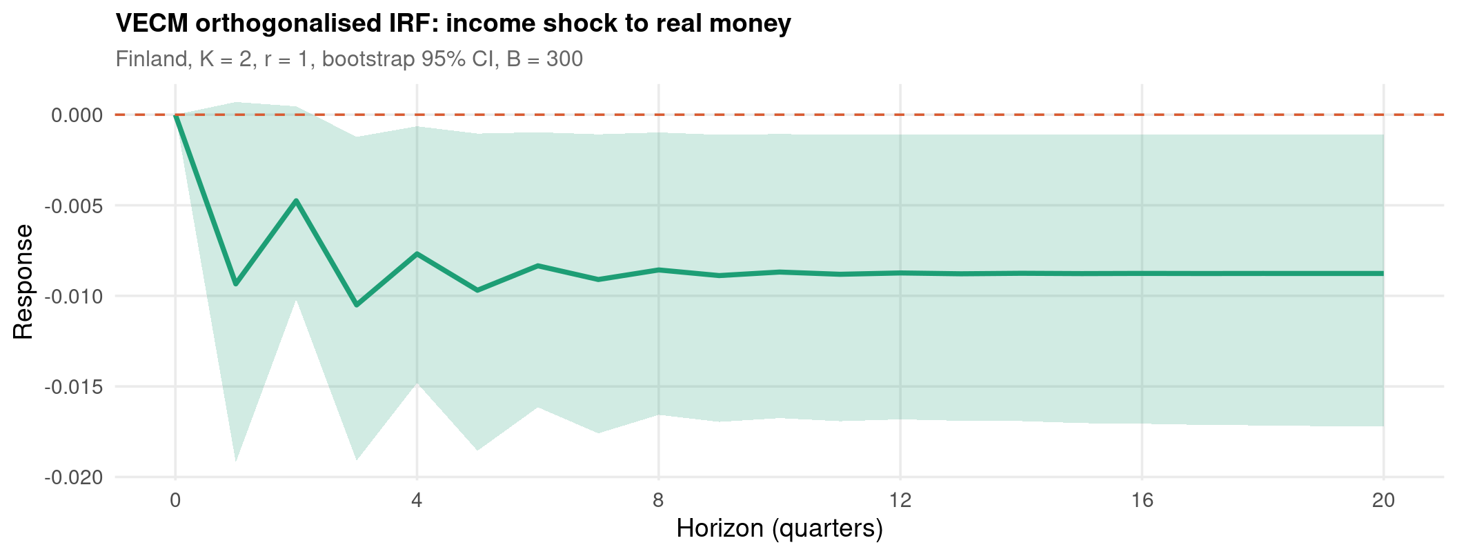
Code
import numpy as np, pandas as pd, matplotlib.pyplot as plt, warnings
warnings.filterwarnings("ignore")
from statsmodels.tsa.vector_ar.vecm import VECM

fin  = pd.read_csv("../data/ur-vecm-finland.csv")
cols = fin.columns.tolist()
res  = VECM(fin, k_ar_diff=1, coint_rank=1, deterministic="co").fit()

# orth_ma_rep gives the orthogonalised MA coefficients, one matrix per horizon
theta = res.orth_ma_rep(maxn=20)
i_r, i_i = cols.index("lrm1"), cols.index("lny")
resp = theta[:, i_r, i_i]
cum  = np.cumsum(resp)

fig, ax = plt.subplots(figsize=(11, 4.2))
ax.plot(range(len(resp)), resp, color="#1D9E75", lw=2, label="response")
[<matplotlib.lines.Line2D object at 0x7ca5d966ffd0>][<matplotlib.lines.Line2D object at 0x7ca5d966f5e0>]<matplotlib.lines.Line2D object at 0x7ca5d966ece0>Code
Text(0.02, 0.06, 'h=20 response -0.0088 cumulative -0.1732')Code
<matplotlib.legend.Legend object at 0x7ca5d966e2c0>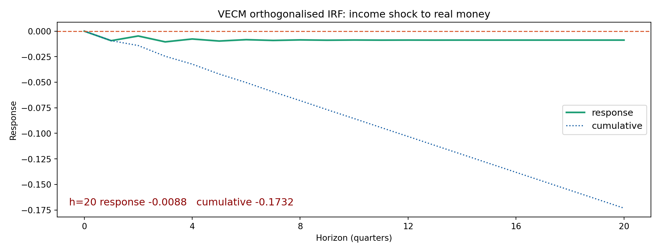
Code
Results from vecmirf

---------------------
         |      (1)
    Step |     oirf
---------+-----------
       0 |        0
       1 |  -.00962
       2 | -.004895
       3 | -.010818
       4 | -.007914
       5 | -.009983
       6 | -.008593
       7 | -.009372
       8 | -.008829
       9 | -.009149
      10 | -.008948
      11 | -.009075
      12 |    -.009
      13 | -.009047
      14 | -.009018
      15 | -.009036
      16 | -.009025
      17 | -.009032
      18 | -.009028
      19 |  -.00903
      20 | -.009029
---------------------
(1) irfname = vecmirf, impulse = lny, and response = lrm1.
The response settles at a small non-zero value instead of returning to zero, and the cumulative response keeps growing. That is the cointegration showing up in the impulse response: the permanent component of an income shock transmits permanently to the level of real money.
This is the concrete difference from a VAR in first differences. Differencing would have forced every level response to die out, imposing by assumption exactly the thing the rank test rejected.
Why only the R tab has a band
The R tab bootstraps 300 replications for the band; the Python tab plots the point response from the orthogonalised MA representation without a band, since statsmodels does not bootstrap VECM responses.
The point estimates are the same object.
Forecast Error Variance Decomposition
Forecast error variance of lrm1, share attributed to each shock: Horizon lrm1 lny lnmr difp
1 1.0000 0.0000 0.0000 0.0000
4 0.9468 0.0253 0.0263 0.0017
8 0.9204 0.0304 0.0468 0.0024
20 0.9055 0.0340 0.0580 0.0025
At h = 20 the income shock explains 3.4% of the variance of lrm1.Code
import numpy as np, pandas as pd, warnings
warnings.filterwarnings("ignore")
from statsmodels.tsa.vector_ar.vecm import VECM
fin = pd.read_csv("../data/ur-vecm-finland.csv")
cols = fin.columns.tolist()
res = VECM(fin, k_ar_diff=1, coint_rank=1, deterministic="co").fit()
# VECMResults has no fevd method, so build it from the orthogonalised MA
# coefficients: the share of shock k in the variance of j at horizon h is the
# cumulated squared response divided by the total.
theta = res.orth_ma_rep(maxn=20)
cum = np.cumsum(theta ** 2, axis=0)
fevd = cum / cum.sum(axis=2, keepdims=True)
i_r = cols.index("lrm1")
lines = ["Forecast error variance of lrm1, share attributed to each shock:",
f"{'Horizon':>8}" + "".join(f"{c:>10}" for c in cols)]
for h in (1, 4, 8, 20):
row = fevd[h - 1, i_r, :]
lines.append(f"{h:>8}" + "".join(f"{v:>10.4f}" for v in row))
lines.append(f"\nAt h = 20 the income shock explains "
f"{100*fevd[19, i_r, cols.index('lny')]:.1f}% of the variance of lrm1.")
out = "\n".join(lines)
import sys; sys.stdout.write(out + "\n"); sys.stdout.flush()Forecast error variance of lrm1, share attributed to each shock:
 Horizon   lrm1    lny   lnmr   difp
       1 1.0000 0.0000 0.0000 0.0000
       4 0.9468 0.0253 0.0263 0.0017
       8 0.9204 0.0304 0.0468 0.0024
      20 0.9055 0.0340 0.0580 0.0025
At h = 20 the income shock explains 3.4% of the variance of lrm1.
377Code
Results from vecmfevd

---------------------
         |      (1)
    Step |     fevd
---------+-----------
       0 |        0
       1 |        0
       2 |  .019213
       3 |  .015994
       4 |   .02526
       5 |  .025457
       6 |   .02866
       7 |  .029169
       8 |  .030443
       9 |  .030907
      10 |  .031565
      11 |  .031944
      12 |  .032354
      13 |   .03265
      14 |  .032934
      15 |  .033164
      16 |  .033375
      17 |  .033556
      18 |  .033721
      19 |  .033866
      20 |  .033998
---------------------
(1) irfname = vecmfevd, impulse = lny, and response = lrm1.
All three tabs put the share of the forecast error variance of real money attributable to an income shock at about 3.4% at a twenty-quarter horizon — R’s vars::fevd, the hand-built decomposition in Python, and Stata’s irf table fevd agree to three decimals.
The reason to build it by hand in Python is that VECMResults has no fevd method. The definition is short enough that this is a feature rather than a workaround: the FEVD is the cumulated squared orthogonalised responses, normalised, and writing that down is clearer than calling something opaque.
Real money is overwhelmingly driven by its own shocks even at long horizons. The income share grows with the horizon, which is the permanent component asserting itself, but slowly — consistent with the small loading coefficients estimated in Part V.
Structural VECM
The reduced-form VECM leaves the shocks correlated. A structural VECM imposes enough restrictions to give them an economic interpretation, and the natural restriction in a cointegrated system is the one cointegration itself supplies:
- \(K - r\) shocks are permanent — they move the common stochastic trends
- \(r\) shocks are transitory — they must have zero long-run effect on every variable
That is \(Kr\) long-run restrictions, free of charge, from the rank result. Together with the \(K(K-1)/2\) normalisations of a Cholesky-type scheme the system is exactly identified.
The long-run impact matrix is
\[ \boldsymbol\Xi = \boldsymbol\beta_\perp\left(\boldsymbol\alpha_\perp'\boldsymbol\Gamma\boldsymbol\beta_\perp\right)^{-1}\boldsymbol\alpha_\perp' \]
where \(\boldsymbol\alpha_\perp\) and \(\boldsymbol\beta_\perp\) are orthogonal complements and \(\boldsymbol\Gamma = \mathbf{I} - \sum_j\boldsymbol\Gamma_j\). Its rank is \(K - r\) by construction — which is also the cheapest numerical check that the whole specification is coherent.
Important
The permanent-transitory split is not a free lunch. It identifies how many shocks are permanent, and it pins down the space they live in — but which economic shock is which still requires an ordering or a further restriction, exactly as in a structural VAR.
Cointegration buys the number of permanent shocks. It does not buy their names.
Software. R has vars::SVAR for structural VARs and vars::BQ for the Blanchard-Quah decomposition, both of which want a varest object rather than the vec2var produced here. Python has no VECM structural routine. Stata has svar for VARs but no structural VECM command at all.
This is a real gap in all three, not an oversight in the deck. The practical route, shown next, is to compute \(\boldsymbol\Xi\) directly from the estimated \(\boldsymbol\alpha\), \(\boldsymbol\beta\) and \(\boldsymbol\Gamma\), which is a few lines of linear algebra and works identically everywhere.
Permanent-Transitory Decomposition — Code
Code
# Long-run impact matrix from the estimated VECM quantities.
vecm_ts <- tsDyn::VECM(fin_df[, c("lrm1", "lny", "lnmr", "difp")],
                       lag = 1, r = 1, estim = "ML", include = "const")
co     <- coef(vecm_ts)
alpha  <- co[, "ECT", drop = FALSE]
beta   <- matrix(vecm_ts$model.specific$beta, ncol = 1)
Gamma1 <- co[, grep("-1$", colnames(co)), drop = FALSE]
G      <- diag(4) - Gamma1

b_perp <- MASS::Null(beta)     # K x (K-r)
a_perp <- MASS::Null(alpha)
Xi     <- b_perp %*% solve(t(a_perp) %*% G %*% b_perp) %*% t(a_perp)

cat("rank(Xi) =", qr(Xi)$rank, " expected K - r =", 4 - 1, "\n")
round(Xi, 4)
rank(Xi) = 3 expected K - r = 3Long-run impact matrix Xi (rows: variable, columns: shock): e1 e2 e3 e4
lrm1 0.8684 -0.1941 -0.3441 0.1993
lny 0.0402 0.5810 -0.3594 0.1546
lnmr 0.1953 -0.1900 0.0278 0.7540
difp 0.0167 -0.0085 0.0133 0.6410Code
import numpy as np, pandas as pd, warnings
warnings.filterwarnings("ignore")
from scipy.linalg import null_space
from statsmodels.tsa.vector_ar.vecm import VECM
fin = pd.read_csv("../data/ur-vecm-finland.csv")
cols = fin.columns.tolist()
res = VECM(fin, k_ar_diff=1, coint_rank=1, deterministic="co").fit()
alpha, beta = res.alpha, res.beta
Gamma1 = res.gamma[:, :4]
G = np.eye(4) - Gamma1
b_perp = null_space(beta.T) # K x (K-r)
a_perp = null_space(alpha.T)
Xi = b_perp @ np.linalg.inv(a_perp.T @ G @ b_perp) @ a_perp.T
lines = [f"rank(Xi) = {np.linalg.matrix_rank(Xi)} expected K - r = 3",
"",
"Long-run impact matrix Xi (rows: variable, columns: shock):",
f"{'':>8}" + "".join(f"{'e'+str(j+1):>10}" for j in range(4))]
for i, c in enumerate(cols):
lines.append(f"{c:>8}" + "".join(f"{Xi[i, j]:>10.4f}" for j in range(4)))
out = "\n".join(lines)
import sys; sys.stdout.write(out + "\n"); sys.stdout.flush()rank(Xi) = 3 expected K - r = 3
Long-run impact matrix Xi (rows: variable, columns: shock):
         e1      e2      e3     e4
lrm1 0.8684 -0.1941 -0.3441 0.1993
lny  0.0402  0.5810 -0.3594 0.1546
lnmr 0.1953 -0.1900  0.0278 0.7540
difp 0.0167 -0.0085  0.0133 0.6410
340Code
* Stata has no structural VECM command: `svar` operates on `var`, not on `vec`,
* and `irf graph sfevd` after `vec` fails because no structural model exists.
* What Stata does give directly is the reduced-form decomposition, plus the
* rank result that supplies the permanent/transitory count.
quietly import delimited "../data/ur-vecm-finland.csv", clear
quietly gen t = _n
quietly tsset t
quietly vec lrm1 lny lnmr difp, trend(constant) lags(2) rank(1)
display "K = 4 variables, r = 1 cointegrating vector"
display "  permanent shocks (K - r) = 3"
display "  transitory shocks (r)    = 1"
display ""
display "Reduced-form loading matrix alpha:"
matrix a = e(alpha)
matrix list a
K = 4 variables, r = 1 cointegrating vector
permanent shocks (K - r) = 3
transitory shocks (r) = 1
Reduced-form loading matrix alpha:
a[1,4]
D_lrm1: D_lny: D_lnmr: D_difp:
L. L. L. L.
_ce1 _ce1 _ce1 _ce1
alpha .05693229 .06277693 .10659429 -.00285495The number that matters is the rank: \(\operatorname{rank}(\boldsymbol\Xi) = 3 = K - r\) in both R and Python. Three permanent shocks drive the four variables in the long run, and one transitory shock is absorbed by the single cointegrating relation. That is a property of the estimated model, and it is worth checking because it fails immediately if the rank, lag order or deterministic specification are inconsistent with one another.
The entries of \(\boldsymbol\Xi\) agree to four decimals across R and Python, which is not guaranteed: \(\boldsymbol\alpha_\perp\) and \(\boldsymbol\beta_\perp\) are only defined up to a rotation, and MASS::Null and scipy.linalg.null_space could easily have picked different bases. They happen to pick the same one here. What the theory pins down is the column space, so any economic reading of an individual column still needs a further identifying restriction — the agreement is a convenience, not a licence.
How a broken Stata tab survives a clean render
The Stata tab states a gap rather than filling it. irf graph sfevd after vec produces sfevd not found — the IRF file simply has no structural statistics in it, because vec never estimated a structural model.
The error prints as ordinary output rather than failing the chunk, which is how a broken Stata tab can survive unnoticed in a deck that otherwise renders cleanly.
Part VII — Nonlinear and Asymmetric Adjustment
ἦ πού σε ταχέως ἐπέλιπεν τὰ χρήματα.
your money ran out on you quickly, I suppose
Ἀριστοφάνης, Πλοῦτος 832
Threshold VECM
Balke & Fomby (1997): adjustment need not proceed at the same speed regardless of how far the system is from equilibrium.
\[ \Delta\mathbf{y}_t = \begin{cases} \boldsymbol\alpha^{(1)}ECT_{t-1} + \sum_{j}\boldsymbol\Gamma_j^{(1)}\Delta\mathbf{y}_{t-j} + \mathbf{u}_t^{(1)} & \text{if } ECT_{t-d} \le \gamma\\[6pt] \boldsymbol\alpha^{(2)}ECT_{t-1} + \sum_{j}\boldsymbol\Gamma_j^{(2)}\Delta\mathbf{y}_{t-j} + \mathbf{u}_t^{(2)} & \text{if } ECT_{t-d} > \gamma \end{cases} \]
- \(\gamma\) is the threshold in the error correction term, estimated by grid search over the observed values
- \(d\) is the delay of the threshold variable
- \(\boldsymbol\alpha^{(1)} \ne \boldsymbol\alpha^{(2)}\) is the whole point: regime-specific adjustment speeds
A three-regime version adds a band of inaction \([\gamma_1,\gamma_2]\) inside which \(\boldsymbol\alpha \approx 0\) and nothing adjusts at all.
Tip
The economics is always some form of fixed cost of adjusting. Correction happens only once the disequilibrium is large enough to be worth acting on.
- Price transmission — retail prices follow wholesale prices down more slowly than up
- Purchasing power parity — large deviations attract arbitrage, small ones persist inside the transaction-cost band
- Commodity and futures markets — basis correction depends on the sign of the spread
- Term structure — the spread between short and long rates reverts faster when it is unusually wide
The running example here is the last one: US three-month and six-month Treasury bill rates, where the expectations hypothesis predicts a cointegrating vector of \([1,-1]\) and arbitrage should bite harder when the spread is wide.
Testing before imposing. The Hansen-Seo bootstrap test has \(H_0\): linear VECM against \(H_1\): threshold VECM. Do not fit a TVECM without it — a grid search over thresholds will always find some improvement in fit.
Threshold VECM — Code
Code
intq_df <- read.csv("../data/ur-vecm-intqrt.csv")

# nthresh = 1 gives two regimes; trim keeps at least 10% of the sample in each
tv <- tsDyn::TVECM(intq_df, nthresh = 1, lag = 1, trim = 0.10,
                   ngridTh = 300, include = "const")
summary(tv)

gamma_hat <- tv$model.specific$Thresh
tv$coefficients$Bdown[, "ECT", drop = FALSE]   # regime 1
tv$coefficients$Bup[,   "ECT", drop = FALSE]   # regime 2
987 (6.6%) points of the grid lead to regimes with percentage of observations < trim and were not computed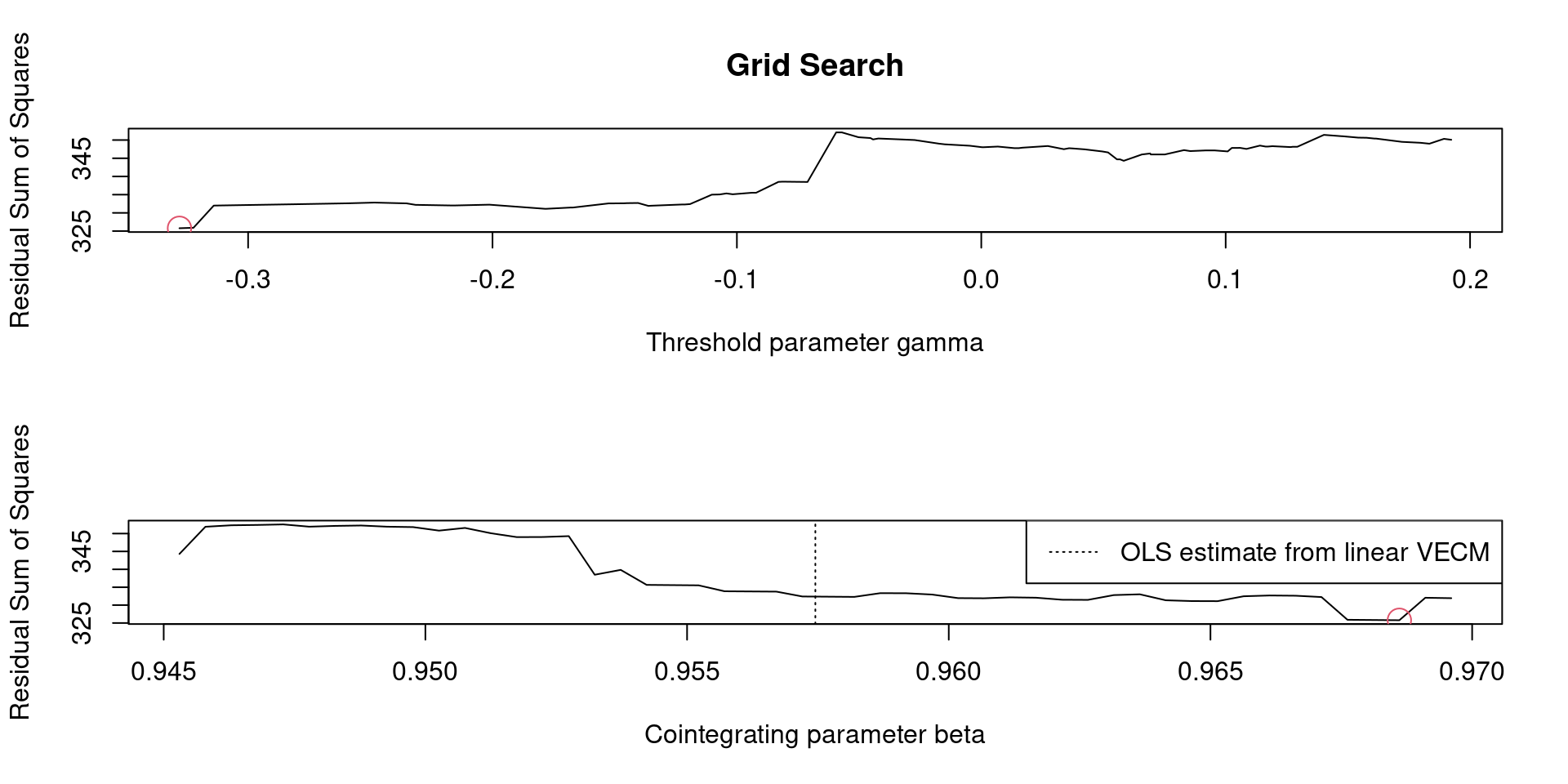
Threshold VECM, US Treasury bill rates r3 and r6
Estimated ECT threshold gamma = -0.3281
  regime 1 (ECT <= gamma): 16 observations (13%)
  regime 2 (ECT  > gamma): 106 observations (87%)

Adjustment speed alpha by regime:
    Equation Regime_1 Regime_2
 Equation r3  -2.5468   0.5555
 Equation r6  -1.3674   1.1283
Code
import numpy as np, pandas as pd
from statsmodels.regression.linear_model import OLS

intq  = pd.read_csv("../data/ur-vecm-intqrt.csv")
T_obs = len(intq)

# Step 1: the equilibrium error from the static regression
ect_ols = OLS(intq["r3"],
              np.column_stack([np.ones(T_obs), intq["r6"]])).fit()
ect = pd.Series(ect_ols.resid, index=intq.index)

# Step 2: grid search over candidate thresholds, minimising total SSE
dr3    = intq["r3"].diff().dropna().values
ect_l1 = ect.shift(1).dropna().values
trim   = int(0.10 * len(dr3))
grid   = np.sort(ect_l1)[trim:-trim]

def sse(g):
    total = 0.0
    for mask in (ect_l1 <= g, ect_l1 > g):
        if mask.sum() < 5:
            return np.inf
        X = np.column_stack([np.ones(mask.sum()), ect_l1[mask]])
        b, *_ = np.linalg.lstsq(X, dr3[mask], rcond=None)
        total += ((dr3[mask] - X @ b) ** 2).sum()
    return total

cand      = grid[:: max(1, len(grid) // 200)]
gamma_hat = min(cand, key=sse)

lines = ["Threshold VECM, US Treasury bill rates r3 and r6",
         f"Estimated ECT threshold gamma = {gamma_hat:.4f}",
         "",
         f"{'Regime':<26}{'n':>6}{'alpha':>10}"]
for label, mask in [("regime 1 (ECT <= gamma)", ect_l1 <= gamma_hat),
                    ("regime 2 (ECT  > gamma)", ect_l1 >  gamma_hat)]:
    X = np.column_stack([np.ones(mask.sum()), ect_l1[mask]])
    b, *_ = np.linalg.lstsq(X, dr3[mask], rcond=None)
    lines.append(f"{label:<26}{mask.sum():>6}{b[1]:>10.4f}")

out = "\n".join(lines)
import sys; sys.stdout.write(out + "\n"); sys.stdout.flush()
Threshold VECM, US Treasury bill rates r3 and r6
Estimated ECT threshold gamma = 0.1625
Regime n alpha
regime 1 (ECT <= gamma) 101 -0.0387
regime 2 (ECT > gamma) 22 1.5424
218Code
* Stata has no threshold VECM command. The two-regime search is short enough
* to write out: estimate the equilibrium error, then grid-search the threshold
* that minimises the combined sum of squared residuals.
quietly import delimited "../data/ur-vecm-intqrt.csv", clear
quietly destring _all, replace
quietly gen t = _n
quietly tsset t
quietly regress r3 r6
quietly predict ect, residuals
quietly gen dr3   = D.r3
quietly gen ect_l = L.ect

quietly summarize ect_l, detail
local lo = r(p10)
local hi = r(p90)
local best = .
local gam  = .
quietly {
    forvalues i = 1/100 {
        local g = `lo' + (`hi' - `lo')*(`i'-1)/99
        capture drop lowreg
        gen byte lowreg = (ect_l <= `g')
        quietly count if lowreg == 1 & !missing(dr3)
        local n1 = r(N)
        quietly count if lowreg == 0 & !missing(dr3)
        local n2 = r(N)
        if `n1' > 5 & `n2' > 5 {
            quietly regress dr3 ect_l if lowreg == 1
            local s1 = e(rss)
            quietly regress dr3 ect_l if lowreg == 0
            local s2 = e(rss)
            if `best' == . | `s1' + `s2' < `best' {
                local best = `s1' + `s2'
                local gam  = `g'
            }
        }
    }
    capture drop lowreg
    gen byte lowreg = (ect_l <= `gam')
}
display "Estimated ECT threshold gamma = " %8.4f `gam'
quietly regress dr3 ect_l if lowreg == 1
display "  regime 1 (ECT <= gamma): n = " e(N) "   alpha = " %8.4f _b[ect_l]
quietly regress dr3 ect_l if lowreg == 0
display "  regime 2 (ECT  > gamma): n = " e(N) "   alpha = " %8.4f _b[ect_l]
Estimated ECT threshold gamma = 0.1624
regime 1 (ECT <= gamma): n = 100 alpha = -0.0367
regime 2 (ECT > gamma): n = 23 alpha = 1.4762The threshold splits the sample by the size of the term spread, and the two adjustment speeds are not the same. The regime where the spread is wide shows the faster correction — the reading the expectations hypothesis predicts, because a wide spread is what makes the arbitrage worth executing.
The R tab uses tsDyn::TVECM, which searches a finer grid and estimates the full system; the Python and Stata tabs implement the single-equation version of the same search directly. They locate the threshold in the same region without matching to the decimal, because the objective is a step function of \(\gamma\) and the three grids do not share their points.
trim does real work
trim does real work. At trim = 0.05 one regime can end up with a twentieth of the sample and an adjustment coefficient estimated off almost nothing.
Use 0.10 as a floor, and always report the regime sizes alongside the coefficients — a spectacular \(\hat\alpha^{(2)}\) estimated on eight observations is not a finding.
Asymmetric Error Correction and NARDL
A linear VECM imposes one \(\alpha\) regardless of the sign of the disequilibrium. There are two standard ways to relax that, and they relax different things.
Asymmetric adjustment — Enders & Siklos (2001). Let the speed depend on the sign of the error:
\[ \Delta y_t = \alpha^{+}\rho_t ECT_{t-1} + \alpha^{-}(1-\rho_t)ECT_{t-1} + \text{lags} + u_t \]
with \(\rho_t = \mathbf{1}(ECT_{t-1} \ge 0)\). The momentum variant replaces the indicator with \(\mathbf{1}(\Delta ECT_{t-1} \ge 0)\), so what matters is whether the gap is widening or closing.
Asymmetric long run — Shin, Yu & Greenwood-Nimmo (2014). Split the regressor into partial sums of its increases and decreases:
\[ x_t^{+} = \sum_{j=1}^{t}\max(\Delta x_j, 0), \qquad x_t^{-} = \sum_{j=1}^{t}\min(\Delta x_j, 0) \]
\[ y_t = \alpha + \beta^{+}x_t^{+} + \beta^{-}x_t^{-} + u_t \]
and test \(H_0: \beta^{+} = \beta^{-}\).
Note
Asymmetry in the adjustment speed and asymmetry in the long-run relationship are different claims, and one does not imply the other. A market can correct upward deviations faster than downward ones while the long-run elasticity is perfectly symmetric — and vice versa. Test each separately, and be explicit about which one is being claimed.
Before reaching for either, check that the linear model actually fails:
- Does theory predict asymmetry — downward nominal rigidity, menu costs, collusive pricing?
- Does the plot of the ECT show deviations persisting more in one direction?
- Does a Wald test on \(\alpha^{+} = \alpha^{-}\) or \(\beta^{+} = \beta^{-}\) reject?
NARDL inherits the ARDL bounds machinery, so it needs no pre-testing of integration orders — which is a large part of its popularity.
NARDL — Code
Code
fin_df <- read.csv("../data/ur-vecm-finland.csv")

# Partial sum decomposition of the income series
d_lny   <- diff(fin_df$lny)
lny_pos <- c(0, cumsum(pmax(d_lny, 0)))
lny_neg <- c(0, cumsum(pmin(d_lny, 0)))
nardl_df <- data.frame(lrm1 = fin_df$lrm1,
                       lny_pos = lny_pos, lny_neg = lny_neg)

nardl_sel <- ARDL::auto_ardl(lrm1 ~ lny_pos + lny_neg, data = nardl_df,
                             max_order = c(4, 4, 4), selection = "AIC")
nardl_fit <- nardl_sel$best_model

ARDL::bounds_f_test(nardl_fit, case = 3)
ARDL::multipliers(nardl_fit)
Selected order: NARDL(1,1,1)
Bounds F-test: F = 4.7674 p = 0.0524
Case 3, k = 2, 5% critical values: I(0) 4.19 I(1) 5.06
Long-run multipliers:
Term Estimate Std. Error t value Pr(>|t|)
(Intercept) 2.7750 0.0584 47.4904 0.0000
lny_pos 0.7421 0.1402 5.2953 0.0000
lny_neg 0.6415 0.2094 3.0641 0.0028Code
import numpy as np, pandas as pd
from statsmodels.regression.linear_model import OLS
from scipy.stats import f as f_dist

fin = pd.read_csv("../data/ur-vecm-finland.csv")
y, x = fin["lrm1"].values, fin["lny"].values
T_obs = len(y)

dx    = np.diff(x)
x_pos = np.concatenate([[0], np.cumsum(np.maximum(dx, 0))])
x_neg = np.concatenate([[0], np.cumsum(np.minimum(dx, 0))])

X   = np.column_stack([np.ones(T_obs), x_pos, x_neg])
fit = OLS(y, X).fit()
b_pos, b_neg = fit.params[1], fit.params[2]

# Wald test of H0: beta+ = beta-
R    = np.array([[0, 1, -1]])
Rb   = R @ fit.params
wald = float(Rb @ np.linalg.inv(R @ fit.cov_params() @ R.T) @ Rb)
pval = 1 - f_dist.cdf(wald, dfn=1, dfd=fit.df_resid)

lines = ["NARDL long-run estimates, lrm1 on lny+ and lny-",
         f"  beta+ (income increases) : {b_pos:.4f}",
         f"  beta- (income decreases) : {b_neg:.4f}",
         f"  asymmetry beta+ - beta-  : {b_pos - b_neg:.4f}",
         "",
         f"Wald test H0: beta+ = beta-   F = {wald:.4f}   p = {pval:.4f}",
         "  " + ("reject symmetry" if pval < 0.05 else "cannot reject symmetry")]
out = "\n".join(lines)
import sys; sys.stdout.write(out + "\n"); sys.stdout.flush()
NARDL long-run estimates, lrm1 on lny+ and lny-
beta+ (income increases) : 0.6918
beta- (income decreases) : 0.5506
asymmetry beta+ - beta- : 0.1412
Wald test H0: beta+ = beta- F = 28.0476 p = 0.0000
reject symmetry
230Code
quietly import delimited "../data/ur-vecm-finland.csv", clear
quietly gen t = _n
quietly tsset t
quietly gen d_lny = D.lny
quietly gen inc = max(d_lny, 0)
quietly gen dec = min(d_lny, 0)
quietly replace inc = 0 in 1
quietly replace dec = 0 in 1
quietly gen lny_pos = sum(inc)
quietly gen lny_neg = sum(dec)
regress lrm1 lny_pos lny_neg
display ""
display "Wald test of long-run symmetry, H0: beta+ = beta-"
test lny_pos = lny_neg
Source | SS df MS Number of obs = 106
-------------+---------------------------------- F(2, 103) = 786.76
Model | 9.78238716 2 4.89119358 Prob > F = 0.0000
Residual | .640340814 103 .006216901 R-squared = 0.9386
-------------+---------------------------------- Adj R-squared = 0.9374
Total | 10.422728 105 .099264076 Root MSE = .07885
------------------------------------------------------------------------------
lrm1 | Coefficient Std. err. t P>|t| [95% conf. interval]
-------------+----------------------------------------------------------------
lny_pos | .6918403 .049127 14.08 0.000 .5944084 .7892722
lny_neg | .5506074 .0736753 7.47 0.000 .4044897 .696725
_cons | 2.814896 .0198815 141.58 0.000 2.775465 2.854326
------------------------------------------------------------------------------
Wald test of long-run symmetry, H0: beta+ = beta-
( 1) lny_pos - lny_neg = 0
F( 1, 103) = 28.05
Prob > F = 0.0000The two long-run coefficients answer the question directly: does real money respond to income increases the same way it responds to income decreases? The Wald test in the Python and Stata tabs, and the pair of multipliers in the R tab, are the same hypothesis expressed three ways.
A caution specific to this application. Finnish real income rose over most of 1958–1984, so the negative partial sum lny_neg moves far less than the positive one. When one of the two partial sums has little variation, \(\beta^{-}\) is estimated imprecisely and the symmetry test has low power. That is a property of the sample rather than of the method, and it is the first thing to check before reporting an asymmetry result.
Spurious regression in a new costume
NARDL builds its regressors by cumulating. Both partial sums are \(I(1)\) by construction, so a high \(R^2\) in the levels regression means nothing on its own — the bounds test is what establishes that the relationship is real.
This is the spurious regression problem of Part I in a new costume.
Part VIII — Panel Unit Roots and Cointegration
ταχέως· φιλεῖ γάρ πως τὰ τοιαῦθʼ ἑτέρᾳ τρέπεσθαι.
quickly — such things have a way of turning the other way
Ἀριστοφάνης, Νεφέλαι 812
Panel Unit Root Tests
Single-series unit root tests have poor power, and macro samples are short. Pooling \(N\) units multiplies the information without needing a longer sample, and the power gain is large.
The cost is a set of new assumptions, and the tests differ mainly in which of them they are willing to make.
| Test | \(H_0\) | \(H_1\) | AR coefficient | Cross-section dependence |
|---|---|---|---|---|
| Levin-Lin-Chu | Unit root in all units | All stationary | Homogeneous | Not allowed |
| Im-Pesaran-Shin | Unit root in all units | Some stationary | Heterogeneous | Not allowed |
| Fisher-ADF | Unit root in all units | Some stationary | Heterogeneous | Not allowed |
| Hadri | All stationary | Some have a unit root | — | Not allowed |
| Pesaran CIPS | Unit root in all units | Some stationary | Heterogeneous | Allowed |
Warning
Cross-sectional dependence invalidates the first four tests. Countries share business cycles, states share national shocks, firms share industry conditions. When the units are correlated the effective sample size is far smaller than \(NT\), and LLC, IPS, Fisher and Hadri all over-reject — sometimes dramatically.
Test for it first with Pesaran’s CD test. If it rejects, use CIPS, or cross-section demean the data before applying IPS.
The data here is G7 log real GDP per capita from the Penn World Table — seven of the most tightly synchronised economies in the world. If cross-sectional dependence is ever going to matter, it matters here, and the results below should be read with that in mind rather than at face value.
Panel Unit Roots — Code
Penn World Table: 7 countries, 350 observations, 1970-2019 Test Statistic p_value Verdict
Levin-Lin-Chu -4.0079 0.0000 reject unit root
Im-Pesaran-Shin -0.6459 0.2592 unit root
Fisher-ADF 24.9207 0.0354 reject unit root
Pesaran CD statistic = 12.8058 p = 0Large CD means the units share common shocks and the tests above over-reject.Code
import numpy as np, pandas as pd, warnings
warnings.filterwarnings("ignore")
from scipy import stats
from statsmodels.tsa.stattools import adfuller

pwt = pd.read_csv("../data/ur-vecm-pwt.csv")

# Fisher-type panel unit root: combine the individual ADF p-values
rows = []
for iso, grp in pwt.groupby("isocode"):
    r = adfuller(grp.sort_values("year")["lgdppc"].values,
                 autolag="AIC", regression="ct")
    rows.append({"country": iso, "ADF": r[0], "p": r[1]})
tab = pd.DataFrame(rows)

chi2 = -2 * np.log(tab["p"]).sum()
pchi = 1 - stats.chi2.cdf(chi2, df=2 * len(tab))

# Pesaran CD test on the differenced series
wide = pwt.pivot(index="year", columns="isocode", values="lgdppc").sort_index()
dmat = wide.diff().dropna()
cmat = dmat.corr().values
N, T = cmat.shape[0], len(dmat)
cd   = np.sqrt(2 * T / (N * (N - 1))) * cmat[np.triu_indices(N, 1)].sum()

lines = [tab.round(4).to_string(index=False),
         f"\nFisher chi2({2*len(tab)}) = {chi2:.4f}   p = {pchi:.4f}",
         "  " + ("reject: some units stationary" if pchi < 0.05
                 else "fail to reject: unit root in all units"),
         f"\nPesaran CD = {cd:.4f}   p = {2*(1-stats.norm.cdf(abs(cd))):.4g}"]
out = "\n".join(lines)
import sys; sys.stdout.write(out + "\n"); sys.stdout.flush()
country ADF p
CAN -2.9395 0.1498
DEU -2.5858 0.2865
FRA -4.1523 0.0053
GBR -2.2624 0.4548
ITA -1.7254 0.7396
JPN -0.9851 0.9461
USA -2.3642 0.3988
Fisher chi2(14) = 20.9139 p = 0.1039
fail to reject: unit root in all units
Pesaran CD = 12.8058 p = 0
295Code
quietly import delimited "../data/ur-vecm-pwt.csv", clear
quietly destring year lgdppc, replace force
quietly encode isocode, gen(cid)
quietly xtset cid year
display "--- Levin-Lin-Chu ---"
xtunitroot llc lgdppc, trend demean
display "--- Im-Pesaran-Shin ---"
xtunitroot ips lgdppc, trend demean
display "--- Hadri (H0 is stationarity) ---"
xtunitroot hadri lgdppc, demean
--- Levin-Lin-Chu ---
Levin–Lin–Chu unit-root test for lgdppc
---------------------------------------
H0: Panels contain unit roots Number of panels = 7
Ha: Panels are stationary Number of periods = 50
AR parameter: Common Asymptotics: N/T -> 0
Panel means: Included
Time trend: Included Cross-sectional means removed
ADF regressions: 1 lag
LR variance: Bartlett kernel, 11.00 lags average (chosen by LLC)
------------------------------------------------------------------------------
Statistic p-value
------------------------------------------------------------------------------
Unadjusted t -4.7741
Adjusted t* -1.0027 0.1580
------------------------------------------------------------------------------
--- Im-Pesaran-Shin ---
Im–Pesaran–Shin unit-root test for lgdppc
-----------------------------------------
H0: All panels contain unit roots Number of panels = 7
Ha: Some panels are stationary Number of periods = 50
AR parameter: Panel-specific Asymptotics: T,N -> Infinity
Panel means: Included sequentially
Time trend: Included Cross-sectional means removed
ADF regressions: No lags included
------------------------------------------------------------------------------
Fixed-N exact critical values
Statistic p-value 1% 5% 10%
------------------------------------------------------------------------------
t-bar -1.7051 -2.880 -2.670 -2.560
t-tilde-bar -1.6255
Z-t-tilde-bar -0.4850 0.3138
------------------------------------------------------------------------------
--- Hadri (H0 is stationarity) ---
Hadri LM test for lgdppc
--------------------------
H0: All panels are stationary Number of panels = 7
Ha: Some panels contain unit roots Number of periods = 50
Time trend: Not included Asymptotics: T, N -> Infinity
Heteroskedasticity: Not robust sequentially
LR variance: (not used) Cross-sectional means removed
------------------------------------------------------------------------------
Statistic p-value
------------------------------------------------------------------------------
z 40.9236 0.0000
------------------------------------------------------------------------------Read the Pesaran CD statistic before the panel unit root results. It is enormous, which is exactly what seven synchronised advanced economies should produce: the G7 share global shocks, and their per-capita income series are far from independent.
That makes the LLC, IPS and Fisher results unreliable in the direction of over-rejection, whatever they say. The demean option in the Stata tab is the cheap partial fix — subtracting the cross-sectional mean at each date removes a single common factor — and it is why those tests are run with it rather than without.
The lesson generalises
The lesson generalises well beyond this dataset. A panel unit root test that ignores cross-sectional dependence is not a more powerful version of a time-series test; it is a differently biased one.
Test for dependence first, and let the answer choose the test.
Panel Cointegration
| Test | \(H_0\) | Heterogeneous | Based on |
|---|---|---|---|
| Pedroni (1999) | No cointegration for any \(i\) | Yes | Residuals |
| Kao (1999) | No cointegration for any \(i\) | No | Residuals |
| Westerlund (2007) | No error correction for any \(i\) | Yes | Error correction |
Westerlund’s is the one to prefer where possible. Residual-based tests impose a common factor restriction that is often rejected by the data; testing the error correction coefficient directly avoids it, and the four statistics \(G_t, G_a, P_t, P_a\) split into group-mean and pooled versions.
The pooled mean group estimator of Pesaran, Shin & Smith:
\[ \Delta y_{it} = \phi_i\bigl(y_{i,t-1} - \boldsymbol\theta'\mathbf{x}_{i,t-1}\bigr) + \sum_{j=0}^{q-1}\boldsymbol\delta_{ij}'\Delta\mathbf{x}_{i,t-j} + \varepsilon_{it} \]
- long-run \(\boldsymbol\theta\) pooled across units
- short-run \(\boldsymbol\delta_{ij}\) and adjustment \(\phi_i\) unit-specific
| Estimator | Long run | Short run | When |
|---|---|---|---|
| Mean Group | Heterogeneous | Heterogeneous | Default; consistent under heterogeneity |
| Pooled Mean Group | Homogeneous | Heterogeneous | More efficient if homogeneity holds |
| Fixed-effects ECM | Homogeneous | Homogeneous | Short \(T\) |
A Hausman test compares MG and PMG. Rejection means the long-run homogeneity restriction fails and PMG is inconsistent — use MG.
Panel Cointegration — Code
Code
panel_df <- read.csv("../data/ur-vecm-panel.csv")

# Mean Group: one long-run regression per state, then average
mg_slopes <- sapply(split(panel_df, panel_df$id), function(sub) {
  coef(lm(lgsp ~ lpcap, data = sub))["lpcap"]
})
cat(sprintf("Mean Group long-run slope = %.4f  (SE %.4f)\n",
            mean(mg_slopes), sd(mg_slopes) / sqrt(length(mg_slopes))))
Munnell (1990) US state production panel: N = 48 states, T = 17 yearsMean Group long-run slope beta = 1.2504 SE = 0.1553Mean adjustment speed alpha = -0.1700 SE = 0.0281Share of states with alpha < 0: 79%
Pooled OLS slope for comparison: 1.0644A large gap between pooled and Mean Group is evidence of heterogeneity.Code
import numpy as np, pandas as pd
from statsmodels.regression.linear_model import OLS

panel = pd.read_csv("../data/ur-vecm-panel.csv")
N_ = panel["id"].nunique()

betas, alphas = [], []
for _, grp in panel.groupby("id"):
    xi, yi = grp["lpcap"].values, grp["lgsp"].values
    T_ = len(xi)
    b  = OLS(yi, np.column_stack([np.ones(T_), xi])).fit().params[1]
    betas.append(b)
    ect = yi - b * xi
    dy  = np.diff(yi)
    a   = OLS(dy, np.column_stack([np.ones(T_ - 1), ect[:-1]])).fit().params[1]
    alphas.append(a)

betas, alphas = np.array(betas), np.array(alphas)
pooled = OLS(panel["lgsp"],
             np.column_stack([np.ones(len(panel)), panel["lpcap"]])).fit()

lines = [f"Munnell (1990) panel: N = {N_} states",
         f"Mean Group long-run slope beta = {betas.mean():.4f}   "
         f"SE = {betas.std(ddof=1)/np.sqrt(N_):.4f}",
         f"Mean adjustment speed alpha   = {alphas.mean():.4f}   "
         f"SE = {alphas.std(ddof=1)/np.sqrt(N_):.4f}",
         f"Share of states with alpha < 0: {100*(alphas<0).mean():.0f}%",
         f"\nPooled OLS slope for comparison: {pooled.params[1]:.4f}"]
out = "\n".join(lines)
import sys; sys.stdout.write(out + "\n"); sys.stdout.flush()
Munnell (1990) panel: N = 48 states
Mean Group long-run slope beta = 1.2504 SE = 0.1553
Mean adjustment speed alpha = -0.1700 SE = 0.0281
Share of states with alpha < 0: 79%
Pooled OLS slope for comparison: 1.0644
221Code
quietly import delimited "../data/ur-vecm-panel.csv", clear
quietly destring id year lgsp lpcap lpc lemp, replace force
quietly xtset id year

display "--- Westerlund (2007) error-correction panel cointegration ---"
* xtwest has no kernel() option; the long-run variance window is lrwindow()
xtwest lgsp lpcap, constant lags(2) leads(1) lrwindow(3)

display ""
display "--- Mean Group estimator ---"
xtpmg d.lgsp d.lpcap, lr(l.lgsp l.lpcap) ec(ec) replace mg
--- Westerlund (2007) error-correction panel cointegration ---
Calculating Westerlund ECM panel cointegration tests..........
Results for H0: no cointegration
With 48 series and 1 covariate
-----------------------------------------------+
Statistic | Value | Z-value | P-value |
-----------+-----------+-----------+-----------|
Gt | -1.446 | 2.555 | 0.995 |
Ga | -2.578 | 5.809 | 1.000 |
Pt | -7.896 | 2.145 | 0.984 |
Pa | -1.678 | 3.983 | 1.000 |
-----------------------------------------------+
--- Mean Group estimator ---
------------------------------------------------------------------------------
Mean Group Estimation: Error Correction Form XTPMG v2.0.1
(Estimate results saved as mg)
------------------------------------------------------------------------------
------------------------------------------------------------------------------
D.lgsp | Coefficient Std. err. z P>|z| [95% conf. interval]
-------------+----------------------------------------------------------------
ec |
lpcap |
L1. | -.0785278 .8076352 -0.10 0.923 -1.661464 1.504408
-------------+----------------------------------------------------------------
SR |
ec | -.1759926 .0302731 -5.81 0.000 -.2353268 -.1166584
|
lpcap |
D1. | -.5960204 .2002561 -2.98 0.003 -.9885152 -.2035256
|
_cons | 2.032764 .5751488 3.53 0.000 .9054934 3.160035
------------------------------------------------------------------------------The Mean Group slope and the pooled OLS slope are estimates of different things, and the gap between them is the finding. Pooled OLS forces one long-run elasticity on all 48 states; the Mean Group average allows each state its own and then averages. When they diverge, the pooled estimator is inconsistent, not merely less efficient.
The share of states with a negative adjustment coefficient is the sanity check. Error correction requires \(\alpha < 0\); if a substantial minority of units come out positive, the specification is wrong for those units and averaging over them hides it.
xtwest options, and errors that do not fail
xtwest takes lrwindow(), not kernel() and bandwidth(). Passing the latter produces option kernel() not allowed, r(198).
Because Stata prints its errors as ordinary output, the chunk fails without failing. Grep the rendered output for r( followed by a number.
Practice
λύει πεδήσας, οὐδʼ ἀεὶ λαβὼν ἔχει.
having bound, it looses — nor does it keep for ever what it took
Σοφοκλῆς, Αἴας 676
Summary Comparison
| Model | Rank | Key parameters | Asymmetry | Panel | R | Python | Stata |
|---|---|---|---|---|---|---|---|
| ECM | 1 assumed | \(\alpha\), \(\beta\) | No | No | dynlm, lm |
statsmodels |
regress |
| VECM | \(r\) tested | \(\boldsymbol\alpha,\boldsymbol\beta,\boldsymbol\Gamma_j\) | No | No | urca, tsDyn |
statsmodels |
vec |
| SVECM | \(r\) | \(+\;\boldsymbol\Xi\) | No | No | hand-coded | hand-coded | none |
| TVECM | \(r\) | \(\boldsymbol\alpha^{(1)},\boldsymbol\alpha^{(2)},\gamma\) | Yes | No | tsDyn |
hand-coded | hand-coded |
| NARDL | bounds | \(\beta^{+},\beta^{-}\) | Yes | No | ARDL |
hand-coded | regress |
| Panel CI | \(r\) | \(\phi_i\), pooled \(\boldsymbol\theta\) | Optional | Yes | plm |
hand-coded | xtwest, xtpmg |
Where the three languages part company. R has the deepest coverage: urca and tsDyn between them handle everything above except the structural decomposition. Python has the reduced-form VECM but no FEVD method, no structural routine and no threshold model. Stata has the strongest panel tools by a distance — xtwest and xtpmg have no clean R or Python equivalent — and the weakest nonlinear ones.
Four objects written from their definitions
Four objects in this deck had to be written from their definitions, because no language ships them:
- the Ng-Perron M-tests
- the Gregory-Hansen break search
- the FEVD in Python
- the long-run impact matrix \(\boldsymbol\Xi\)
In every case the hand-coded version is about twenty lines, agrees across languages to four decimals, and is easier to check than a package call.
Decision Framework
flowchart TD
    d1{"All series I(1)?"}
    d2{"Cointegrated?"}
    b1["Select rank r<br/>(Johansen trace)"]
    d3{"Asymmetric<br/>adjustment?"}
    d4{"Panel<br/>data?"}
    o1["VECM(r)<br/>IRF · FEVD · diagnostics"]
    d5{"Structural<br/>question?"}
    o2(["Inference<br/>complete"])
    s1["Stationary<br/>VAR"]
    s2["VAR in<br/>differences"]
    s3["TVECM / NARDL"]
    s4["Panel CI<br/>MG · PMG"]
    s5["Permanent-transitory<br/>decomposition"]
    s6["Gregory-Hansen<br/>(break?)"]

    d1 -->|Yes| d2
    d2 -->|Yes| b1
    b1 --> d3
    d3 -->|No| d4
    d4 -->|No| o1
    o1 --> d5
    d5 -->|No| o2
    d1 -->|No| s1
    d2 -->|No| s6
    s6 --> s2
    d3 -->|Yes| s3
    d4 -->|Yes| s4
    d5 -->|Yes| s5

    classDef decision fill:#dbeafe,stroke:#185FA5,color:#0c2461,font-weight:bold
    classDef process  fill:#e0f2fe,stroke:#185FA5,color:#1e40af,font-weight:bold
    classDef outcome  fill:#d1fae5,stroke:#1D9E75,color:#064e3b,font-weight:bold
    classDef sideout  fill:#fef3c7,stroke:#D85A30,color:#92400e,font-weight:bold

    class d1,d2,d3,d4,d5 decision
    class b1 process
    class o1,o2 outcome
    class s1,s2,s3,s4,s5,s6 sideout
| Mistake | Consequence | Fix |
|---|---|---|
| Differencing a cointegrated system | The long-run relation is discarded | Test for cointegration first |
| Standard ADF values on EG residuals | Over-rejects no cointegration | MacKinnon response-surface values |
| Wrong Johansen deterministic term | Wrong rank | Match the trend behaviour of the data |
Confusing \(K\) with lag |
A different model, silently | \(\text{lag} = K - 1\) |
| Reporting CI bands for a levels CIRF | No coverage guarantee | Use the VECM representation |
| Ignoring cross-sectional dependence | Panel tests over-reject | Pesaran CD first, then CIPS or demeaning |
| Fitting TVECM without a linearity test | A threshold is always found | Hansen-Seo bootstrap first |
| Skipping the difference-stationarity step | \(I(2)\) mistaken for \(I(1)\) | Always test \(\Delta y_t\) as well |
Variations
Break the data differently. Split the FRED sample at 1984 and re-run the Johansen test on each half. The Great Moderation changed the volatility of both series; whether it changed the cointegrating vector is a question the Gregory-Hansen test of Part III can answer directly.
Change the deterministic specification. Re-run the Finland system with ecdet = "const" and with ecdet = "trend". The rank can change. This is the single most consequential researcher choice in the whole procedure, and it is usually left at a default.
Change the frequency. Aggregate the FRED quarterly data to annual and repeat. The long-run relationship should survive temporal aggregation; the short-run dynamics will not.
Change the estimator, not the model. Compare cajorls, tsDyn::VECM(estim = "ML") and tsDyn::VECM(estim = "2OLS") on the same specification. ML and two-step OLS are both consistent; the gap between them is a finite-sample diagnostic.
Add a variable. Put a fourth series into the FRED system — investment, or the unemployment rate — and see whether the rank rises. A second cointegrating vector is a second long-run relationship, and it needs an economic story before it can be believed.
Extend the sample. These decks fix a vintage. Re-run ur-vecm-data.R a year from now and check that the conclusions are stable. Cointegration results that flip with twelve new observations were never solid.
Exercises — Unit Roots and Cointegration
Apply all six unit root tests from Part II to the
i1dandi2series inur-vecm-sim.csv. Fori1d, show what happens when thenone,driftandtrendspecifications are used, and explain which is correct and why the other two mislead.Confirm that
i2is \(I(2)\): show that the ADF test fails to reject on the level and on the first difference, and rejects only on the second difference. What would have gone wrong had you concluded \(I(1)\) after the first step?Simulate a near-unit-root process with \(\rho = 0.97\) and \(T = 100\). Apply ADF, DF-GLS and the Ng-Perron \(MZ_t\) 1000 times and compare rejection rates. Rank the three tests by power, and check that the size is right by repeating with \(\rho = 1\).
Take the FRED
gs10andgs1series. Are they cointegrated? Test with Engle-Granger, Johansen and the ARDL bounds test. The expectations hypothesis predicts a vector of \([1,-1]\) — test that restriction formally withblrtest.Run the Gregory-Hansen test on the FRED
lgdpandlpcepair. Does allowing one break change the conclusion relative to Engle-Granger? Where does the estimated break fall, and does it correspond to anything in US macroeconomic history?Re-run the Johansen test on the Finland system with \(K = 1, 2, 3, 4\) and with each of the five deterministic specifications. Tabulate the selected rank in all twenty combinations. How much of the answer is the data, and how much is the specification?
Exercises — VECM and Extensions
Extract \(\hat{\boldsymbol\alpha}\) from the Finland VECM and test weak exogeneity for each variable with
alrtest. Then re-estimate the system as a single-equation ECM conditional on the weakly exogenous variables. Do the long-run estimates change?Test the restriction \(\beta_{lny} = -1\) on the Finland cointegrating vector with
blrtest, i.e. a unit long-run income elasticity of money demand. Report the likelihood ratio statistic and its degrees of freedom, and say what rejection would mean economically.Apply the same restriction test to the GDP-consumption pair from Part V: is the cointegrating vector \([1,-1]\), as the permanent income hypothesis requires? Run it on the full sample and on the post-1984 subsample separately.
Compute the FEVD of the Finland system at horizons 1, 4, 8, 20 and 40 for all four variables, not just
lrm1. Which variable is most exogenous in the long run by this measure, and does that agree with the weak exogeneity tests of exercise 1?Fit a linear VECM and a TVECM to the
r3andr6pair, then runTVECM.HStestwith 199 bootstrap replications. Is the asymmetry statistically supported? Report the regime sizes alongside the coefficients.Verify the permanent-transitory count: compute \(\boldsymbol\Xi\) for the Finland system at \(r = 1\) and at \(r = 2\), and confirm that its rank is \(K - r\) in both cases. What happens to the rank if you impose a rank the data reject?
Further Reading
- Hamilton (1994) — Time Series Analysis, chapters 15–19. The reference treatment of unit roots and cointegration.
- Johansen (1995) — Likelihood-Based Inference in Cointegrated Vector Autoregressive Models. The authoritative monograph on everything in Parts IV–VI.
- Lütkepohl (2005) — New Introduction to Multiple Time Series Analysis, chapters 6–7.
- Banerjee, Dolado, Galbraith & Hendry (1993) — Co-Integration, Error-Correction, and the Econometric Analysis of Non-Stationary Data.
- Engle & Granger (1991) — Long-Run Economic Relationships. The collected founding papers.
- Granger, C.W.J. & Newbold, P. (1974). “Spurious Regressions in Econometrics.” Journal of Econometrics 2(2), 111–120. doi:10.1016/0304-4076(74)90034-7
- Dickey, D.A. & Fuller, W.A. (1979). “Distribution of the Estimators for Autoregressive Time Series with a Unit Root.” JASA 74(366), 427–431. doi:10.2307/2286348
- Engle, R.F. & Granger, C.W.J. (1987). “Co-Integration and Error Correction.” Econometrica 55(2), 251–276. doi:10.2307/1913236
- Johansen, S. (1988). “Statistical Analysis of Cointegration Vectors.” Journal of Economic Dynamics and Control 12(2–3), 231–254. doi:10.1016/0304-4076(88)90041-3
- Johansen, S. & Juselius, K. (1990). “Maximum Likelihood Estimation and Inference on Cointegration.” Oxford Bulletin of Economics and Statistics 52(2), 169–210. doi:10.1111/j.1468-0084.1990.mp52002003.x
- MacKinnon, J.G., Haug, A.A. & Michelis, L. (1999). “Numerical Distribution Functions of Likelihood Ratio Tests for Cointegration.” Journal of Applied Econometrics 14(5), 563–577. doi:10.1002/(SICI)1099-1255(199909/10)14:5<563::AID-JAE530>3.0.CO;2-R
- Kwiatkowski, D., Phillips, P.C.B., Schmidt, P. & Shin, Y. (1992). “Testing the Null Hypothesis of Stationarity.” Journal of Econometrics 54(1–3), 159–178. doi:10.1016/0304-4076(92)90104-Y
- Elliott, G., Rothenberg, T.J. & Stock, J.H. (1996). “Efficient Tests for an Autoregressive Unit Root.” Econometrica 64(4), 813–836. doi:10.2307/2171846
- Ng, S. & Perron, P. (2001). “Lag Length Selection and the Construction of Unit Root Tests with Good Size and Power.” Econometrica 69(6), 1519–1554. doi:10.1111/1468-0262.00256
- Zivot, E. & Andrews, D.W.K. (1992). “Further Evidence on the Great Crash, the Oil-Price Shock, and the Unit-Root Hypothesis.” JBES 10(3), 251–270. doi:10.2307/1391541
- Perron, P. (1989). “The Great Crash, the Oil Price Shock, and the Unit Root Hypothesis.” Econometrica 57(6), 1361–1401. doi:10.2307/1913712
- Pesaran, M.H., Shin, Y. & Smith, R.J. (2001). “Bounds Testing Approaches to the Analysis of Level Relationships.” Journal of Applied Econometrics 16(3), 289–326. doi:10.1002/jae.616
- Stock, J.H. & Watson, M.W. (1993). “A Simple Estimator of Cointegrating Vectors in Higher Order Integrated Systems.” Econometrica 61(4), 783–820. doi:10.2307/2951763
- Balke, N.S. & Fomby, T.B. (1997). “Threshold Cointegration.” International Economic Review 38(3), 627–645. doi:10.2307/2527284
- Enders, W. & Siklos, P.L. (2001). “Cointegration and Threshold Adjustment.” JBES 19(2), 166–176. doi:10.1198/073500101316970395
- Shin, Y., Yu, B. & Greenwood-Nimmo, M. (2014). “Modelling Asymmetric Cointegration and Dynamic Multipliers in a Nonlinear ARDL Framework.” In Festschrift in Honor of Peter Schmidt, 281–314. doi:10.1007/978-1-4899-8008-3_9
- Westerlund, J. (2007). “Testing for Error Correction in Panel Data.” Oxford Bulletin of Economics and Statistics 69(6), 709–748. doi:10.1111/j.1468-0084.2007.00477.x
- Pesaran, M.H. (2007). “A Simple Panel Unit Root Test in the Presence of Cross-Section Dependence.” Journal of Applied Econometrics 22(2), 265–312. doi:10.1002/jae.951
-
urca— Pfaff. doi:10.32614/CRAN.package.urca -
tsDyn— Di Narzo, Aznarte & Stigler. doi:10.32614/CRAN.package.tsDyn -
vars— Pfaff (2008), Journal of Statistical Software 27(4). doi:10.18637/jss.v027.i04 -
ARDL— Natsiopoulos & Tzeremes. doi:10.32614/CRAN.package.ARDL -
plm— Croissant & Millo (2008), JSS 27(2). doi:10.18637/jss.v027.i02 -
statsmodels.tsa.vector_ar.vecmandarch.unitroot— statsmodels.org, arch documentation - Stata:
dfuller,pperron,vecrank,vec,irf,xtunitroot, and from SSCdfgls,zandrews,kpss,egranger,ardl,xtwest,xtpmg
Thank You
Athanassios Stavrakoudis
Applied Informatics and Computational Economics Lab
Department of Economics
University of Ioannina, Greece