Vector Autoregressive Models

& Local Projections in Econometrics
using R, Python & Stata

Applied Informatics and Computational Economics Lab

2026-06-29

The VAR Family — A Road Map

The VAR Family at a Glance

Model Key Idea Best Use Case
VAR Joint dynamics of \(K\) series Baseline multivariate TS
SVAR Theory-based identification Monetary/financial shocks
FAVAR Factors summarise large datasets Macro with many indicators
BVAR Priors shrink parameters Large-dimensional forecasting
TVAR Regime switching Crisis vs normal times
GVAR Multi-country linkages Spillovers, contagion
PVAR Panel dynamics Firms, regions, countries
QVAR Quantile responses Tail-risk analysis
LP Non-parametric IRFs Robust IRFs, nonlinearities
Sparse VAR Penalised estimation High-dimensional systems

Running example throughout:

 Canada (R vars package)
 84 quarterly observations, 1980Q1–2000Q4

Variable Description
e Employment (log)
prod Labour productivity (log)
rw Real wages (log)
U Unemployment rate


Also used: Lütkepohl (2005) West German macro data for Stata examples; US macro data (statsmodels) for Python.

Part I — VAR Foundations

The VAR(\(p\)) Model

Reduced-form VAR(\(p\)):

\[\mathbf{y}_t = \mathbf{c} + \mathbf{A}_1\mathbf{y}_{t-1} + \cdots + \mathbf{A}_p\mathbf{y}_{t-p} + \mathbf{u}_t, \qquad \mathbf{u}_t \sim \mathcal{WN}(\mathbf{0},\, \Sigma_u)\]

  • \(\mathbf{y}_t\): \(K \times 1\) vector of endogenous variables at time \(t\)
  • \(\mathbf{A}_j\): \(K \times K\) coefficient matrices (\(j = 1,\ldots,p\))
  • \(\mathbf{u}_t\): \(K \times 1\) white-noise error vector; \(\Sigma_u\) positive definite
  • Total parameters: \(K^2 p + K\) — grows quickly in \(K\) and \(p\)

Companion form (VAR(1) representation):

\[\mathbf{Y}_t = \mathbf{C} + \mathbf{A}\,\mathbf{Y}_{t-1} + \mathbf{U}_t, \qquad \mathbf{Y}_t = \begin{pmatrix}\mathbf{y}_t \\ \vdots \\ \mathbf{y}_{t-p+1}\end{pmatrix},\quad \mathbf{A} = \begin{pmatrix}\mathbf{A}_1 & \cdots & \mathbf{A}_p \\ \mathbf{I} & & \mathbf{0}\end{pmatrix}\]

Stability condition: all eigenvalues of \(\mathbf{A}\) lie inside the unit circle.

Note

Sims (1980) Critique

Classical structural models imposed a priori exclusion restrictions that were “incredible.” Sims proposed the unrestricted VAR as an atheoretical alternative, letting the data speak. All variables are treated symmetrically — there is no arbitrary distinction between endogenous and exogenous.

Tip

MA(\(\infty\)) representation

For a stable VAR(\(p\)), the Wold representation is: \[\mathbf{y}_t = \boldsymbol{\mu} + \sum_{h=0}^{\infty}\boldsymbol{\Phi}_h\,\mathbf{u}_{t-h}, \qquad \boldsymbol{\Phi}_0 = \mathbf{I}_K, \quad \boldsymbol{\Phi}_h = \sum_{j=1}^{p}\mathbf{A}_j\boldsymbol{\Phi}_{h-j}\]

The matrices \(\boldsymbol{\Phi}_h\) are the impulse-response coefficients at horizon \(h\).

Criterion Formula Penalty
AIC \(\ln|\hat\Sigma_u| + \frac{2}{T}K^2 p\) Lightest
HQ \(\ln|\hat\Sigma_u| + \frac{2\ln\ln T}{T}K^2 p\) Medium
BIC / SC \(\ln|\hat\Sigma_u| + \frac{\ln T}{T}K^2 p\) Heaviest

Rules of thumb: AIC tends to over-fit; BIC is consistent; HQ intermediate. Always confirm lag adequacy via residual autocorrelation (Portmanteau test).

Impulse Responses & Variance Decomposition

Orthogonalised IRF (OIRF):

\[\boldsymbol{\Theta}_h = \boldsymbol{\Phi}_h\,\mathbf{P}, \qquad \mathbf{P} = \operatorname{chol}(\hat\Sigma_u), \quad \mathbf{PP}' = \hat\Sigma_u\]

  • \(\mathbf{P}\) is the lower Cholesky factor of the estimated error covariance
  • Column \(k\) of \(\boldsymbol{\Theta}_h\): response of all variables to a one standard deviation shock in variable \(k\)
  • Causal ordering matters: variable ordered first cannot be affected contemporaneously by variables ordered later

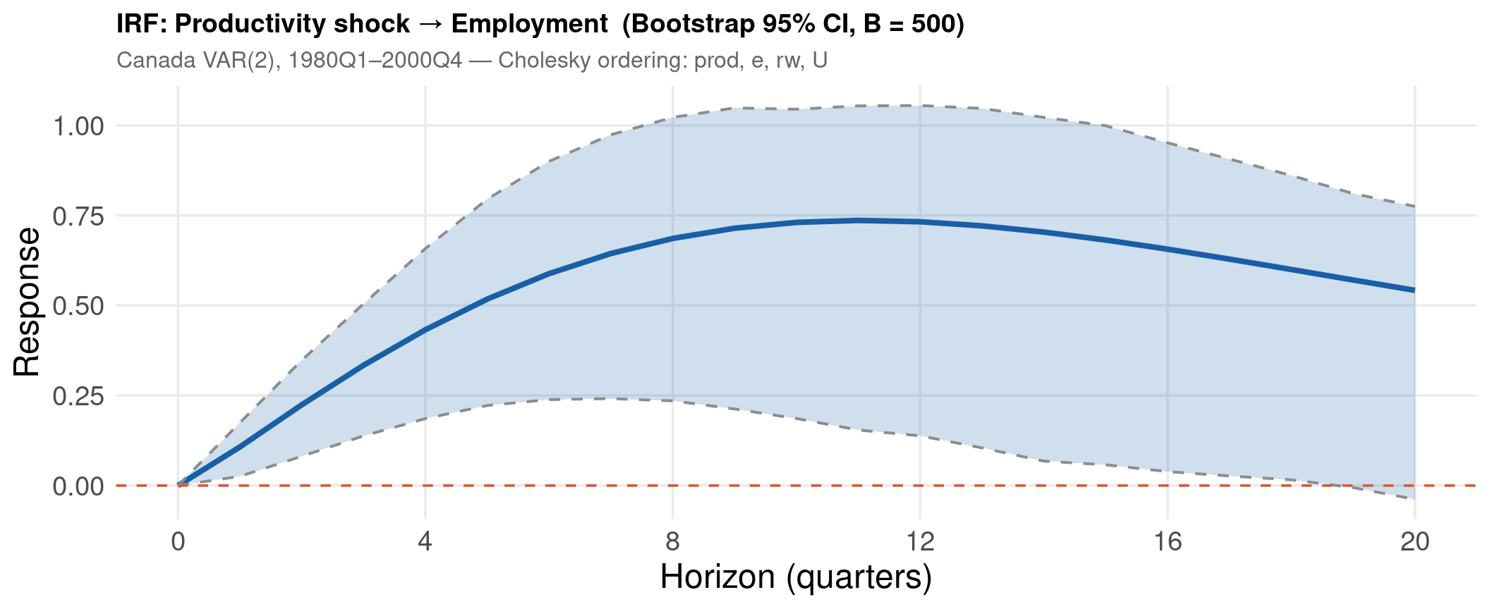
Bootstrap CI (Kilian 1998, residual resampling):

  1. Fit VAR(\(p\)) → \(\hat\mathbf{A}_j\), residuals \(\hat\mathbf{u}_t\)
  2. Resample \(\hat\mathbf{u}_t\) with replacement → \(\mathbf{u}_t^*\)
  3. Reconstruct \(\mathbf{y}^*\) → re-estimate → compute OIRF\(^*(h)\)
  4. Repeat \(B\) times → percentile band at each horizon

Forecast Error Variance Decomposition:

\[\omega_{jk,h} = \frac{\displaystyle\sum_{i=0}^{h-1}\bigl(\boldsymbol{\Theta}_i\bigr)^2_{jk}}{\operatorname{MSE}(y_{j,t+h})}, \qquad \sum_{k=1}^K \omega_{jk,h} = 1\]

\(\omega_{jk,h}\): fraction of the \(h\)-step forecast error variance of variable \(j\) explained by shocks to variable \(k\).

Tip

Reading a FEVD table

If \(\omega_{jj,h} \approx 1\) at all horizons, variable \(j\) is nearly exogenous — its variance is dominated by own shocks. If \(\omega_{jk,h}\) grows with \(h\) for \(k \ne j\), the inter-variable linkage matters more at longer horizons (typical in monetary policy settings).

Variable \(x\) Granger-causes \(y\) if past values of \(x\) improve forecasts of \(y\) beyond what past \(y\) alone provides.

Test in VAR: \(H_0\): \(A^{xy}_{1} = A^{xy}_{2} = \cdots = A^{xy}_{p} = \mathbf{0}\) — the block of coefficients of \(x\) in the \(y\)-equation are jointly zero.

Implemented via Wald test: causality(var_fit, cause = "x") in R; vargranger in Stata.

Warning

Granger causality is a predictive concept, not structural causality. Rejection means \(x\) contains incremental predictive information about \(y\) — it does not imply \(x\) causes \(y\) in a counterfactual sense.

Code — VAR Estimation

library(vars)
data(Canada)

# 1. Lag selection
vs <- VARselect(Canada, lag.max = 8, type = "const")
vs$selection          # AIC, HQ, SC, FPE selections
AIC(n)  HQ(n)  SC(n) FPE(n) 
     3      2      1      3 
# 2. Estimate VAR(2) — chosen by AIC
var_fit <- VAR(Canada, p = 2, type = "const")

# 3. Coefficient table for the employment (e) equation
round(coef(var_fit)$e, 4)
         Estimate Std. Error t value Pr(>|t|)
e.l1       1.6378     0.1500 10.9181   0.0000
prod.l1    0.1673     0.0611  2.7360   0.0078
rw.l1     -0.0631     0.0552 -1.1427   0.2569
U.l1       0.2656     0.2028  1.3096   0.1944
e.l2      -0.4971     0.1595 -3.1163   0.0026
prod.l2   -0.1017     0.0661 -1.5385   0.1282
rw.l2      0.0038     0.0555  0.0692   0.9450
U.l2       0.1327     0.2073  0.6400   0.5242
const   -136.9984    55.8481 -2.4531   0.0166
Lag selection criteria:
AIC(n)  HQ(n)  SC(n) FPE(n) 
     3      2      1      3 
VAR(2) — Employment equation coefficients (Canada data)
Estimate Std. Error t value Pr(>|t|)
e.l1 1.6378 0.1500 10.9181 0.0000
prod.l1 0.1673 0.0611 2.7360 0.0078
rw.l1 -0.0631 0.0552 -1.1427 0.2569
U.l1 0.2656 0.2028 1.3096 0.1944
e.l2 -0.4971 0.1595 -3.1163 0.0026
prod.l2 -0.1017 0.0661 -1.5385 0.1282
rw.l2 0.0038 0.0555 0.0692 0.9450
U.l2 0.1327 0.2073 0.6400 0.5242
const -136.9984 55.8481 -2.4531 0.0166
import numpy as np
import pandas as pd
from statsmodels.datasets import macrodata
from statsmodels.tsa.vector_ar.var_model import VAR

# US macro data (statsmodels built-in) — quarterly, 1959Q1–2009Q3
data = macrodata.load_pandas().data
Y = pd.DataFrame({
    "dlgdp":  np.log(data["realgdp"]).diff(),
    "dlcons": np.log(data["realcons"]).diff(),
    "dlinv":  np.log(data["realinv"]).diff(),
}).dropna()

# Lag selection
model  = VAR(Y)
lag_ic = model.select_order(maxlags=8)
print(lag_ic.summary())
 VAR Order Selection (* highlights the minimums) 
=================================================
      AIC         BIC         FPE         HQIC   
-------------------------------------------------
0      -27.72      -27.66   9.194e-13      -27.69
1     -28.03*     -27.82*  6.735e-13*     -27.94*
2      -28.02      -27.66   6.810e-13      -27.87
3      -28.01      -27.51   6.829e-13      -27.81
4      -28.01      -27.35   6.850e-13      -27.74
5      -28.00      -27.19   6.956e-13      -27.67
6      -27.96      -27.00   7.228e-13      -27.57
7      -27.93      -26.82   7.407e-13      -27.48
8      -27.93      -26.66   7.475e-13      -27.41
-------------------------------------------------
# Estimate VAR(2)
res = model.fit(2, trend="c")
print(res.summary())
  Summary of Regression Results   
==================================
Model:                         VAR
Method:                        OLS
Date:           Κυρ, 02, Αυγ, 2026
Time:                     16:17:33
--------------------------------------------------------------------
No. of Equations:         3.00000    BIC:                   -27.5830
Nobs:                     200.000    HQIC:                  -27.7892
Log likelihood:           1962.57    FPE:                7.42129e-13
AIC:                     -27.9293    Det(Omega_mle):     6.69358e-13
--------------------------------------------------------------------
Results for equation dlgdp
============================================================================
               coefficient       std. error           t-stat            prob
----------------------------------------------------------------------------
const             0.001527         0.001119            1.365           0.172
L1.dlgdp         -0.279435         0.169663           -1.647           0.100
L1.dlcons         0.675016         0.131285            5.142           0.000
L1.dlinv          0.033219         0.026194            1.268           0.205
L2.dlgdp          0.008221         0.173522            0.047           0.962
L2.dlcons         0.290458         0.145904            1.991           0.047
L2.dlinv         -0.007321         0.025786           -0.284           0.776
============================================================================

Results for equation dlcons
============================================================================
               coefficient       std. error           t-stat            prob
----------------------------------------------------------------------------
const             0.005460         0.000969            5.634           0.000
L1.dlgdp         -0.100468         0.146924           -0.684           0.494
L1.dlcons         0.268640         0.113690            2.363           0.018
L1.dlinv          0.025739         0.022683            1.135           0.257
L2.dlgdp         -0.123174         0.150267           -0.820           0.412
L2.dlcons         0.232499         0.126350            1.840           0.066
L2.dlinv          0.023504         0.022330            1.053           0.293
============================================================================

Results for equation dlinv
============================================================================
               coefficient       std. error           t-stat            prob
----------------------------------------------------------------------------
const            -0.023903         0.005863           -4.077           0.000
L1.dlgdp         -1.970974         0.888892           -2.217           0.027
L1.dlcons         4.414162         0.687825            6.418           0.000
L1.dlinv          0.225479         0.137234            1.643           0.100
L2.dlgdp          0.380786         0.909114            0.419           0.675
L2.dlcons         0.800281         0.764416            1.047           0.295
L2.dlinv         -0.124079         0.135098           -0.918           0.358
============================================================================

Correlation matrix of residuals
             dlgdp    dlcons     dlinv
dlgdp     1.000000  0.603316  0.750722
dlcons    0.603316  1.000000  0.131951
dlinv     0.750722  0.131951  1.000000
frause lutkepohl2, clear
tsset qm

* First differences of log variables
generate dln_inv = D.ln_inv
generate dln_inc = D.ln_inc
generate dln_con = D.ln_con
drop if missing(dln_inv)

* Lag selection (information criteria)
varsoc dln_inv dln_inc dln_con, maxlag(8)

* Estimate VAR(2) — BIC-chosen lag
var dln_inv dln_inc dln_con, lags(1/2)

* Summary statistics and Granger causality
vargranger

Code — Impulse Response Functions

Code
set.seed(14159)
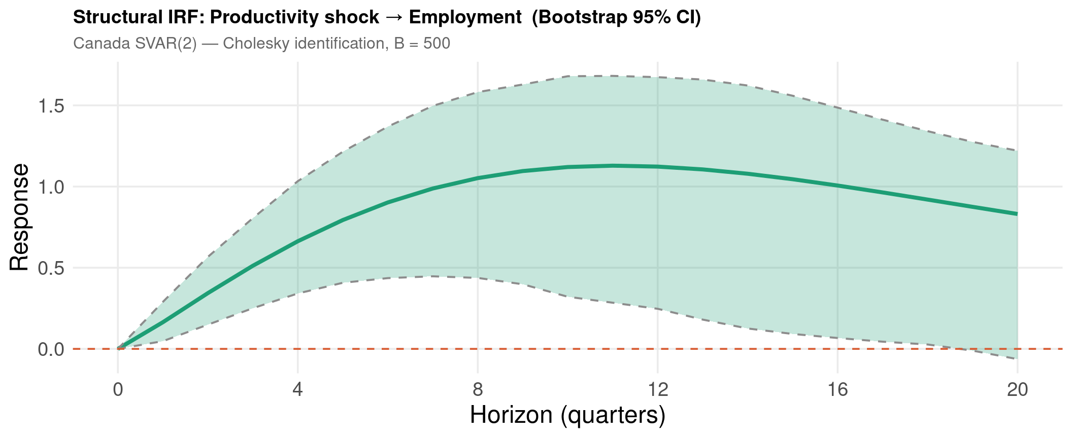
irf_fit <- vars::irf(var_fit, impulse = "prod", response = c("e", "rw", "U"),
                     n.ahead = 20, boot = TRUE, runs = 500, ci = 0.95)

# Tidy the prod → e response for ggplot
irf_tbl <- tibble(
  h    = 0:20,
  irf  = as.numeric(irf_fit$irf$prod[, "e"]),
  lo95 = as.numeric(irf_fit$Lower$prod[, "e"]),
  hi95 = as.numeric(irf_fit$Upper$prod[, "e"])
)

ggplot(irf_tbl, aes(x = h)) +
  geom_ribbon(aes(ymin = lo95, ymax = hi95), fill = col_main, alpha = 0.20) +
  geom_line(aes(y = irf),  colour = col_main,  linewidth = 1.4) +
  geom_line(aes(y = lo95), colour = col_muted, linewidth = 0.7, linetype = "dashed") +
  geom_line(aes(y = hi95), colour = col_muted, linewidth = 0.7, linetype = "dashed") +
  geom_hline(yintercept = 0, colour = col_accent, linetype = "dashed") +
  scale_x_continuous(breaks = seq(0, 20, 4)) +
  labs(
    title    = "IRF: Productivity shock → Employment  (Bootstrap 95% CI, B = 500)",
    subtitle = "Canada VAR(2), 1980Q1–2000Q4 — Cholesky ordering: prod, e, rw, U",
    x        = "Horizon (quarters)",
    y        = "Response"
  ) +
  theme(text = element_text(size = 18))

Code
import numpy as np
import pandas as pd
import matplotlib.pyplot as plt
from statsmodels.datasets import macrodata
from statsmodels.tsa.vector_ar.var_model import VAR

# Rebuild data and model (each chunk is self-contained)
data = macrodata.load_pandas().data
Y_irf = pd.DataFrame({
    "dlgdp":  np.log(data["realgdp"]).diff(),
    "dlcons": np.log(data["realcons"]).diff(),
    "dlinv":  np.log(data["realinv"]).diff(),
}).dropna()

res_irf = VAR(Y_irf).fit(2, trend="c")

irf_py = res_irf.irf(periods=20)
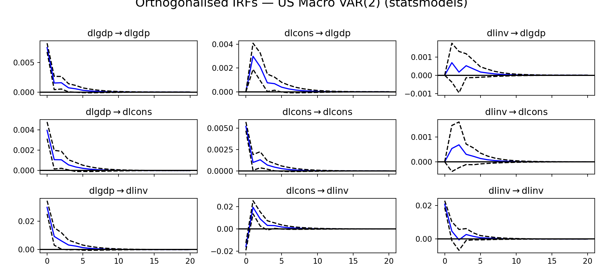
fig = irf_py.plot(orth=True, figsize=(11, 5))
plt.suptitle("Orthogonalised IRFs — US Macro VAR(2) (statsmodels)",
             fontsize=16, y=1.01)
plt.tight_layout()
plt.show()

Code
frause lutkepohl2, clear
tsset qm
generate dln_inv = D.ln_inv
generate dln_inc = D.ln_inc
generate dln_con = D.ln_con
drop if missing(dln_inv)

var dln_inv dln_inc dln_con, lags(1/2)

* Compute and store IRFs
irf create var_irf, step(20) set(myirf) replace
irf graph oirf, impulse(dln_inv) response(dln_inc) ///
    title("OIRF: Investment → Income (Lütkepohl data)") ///
    yline(0, lpattern(dash) lcolor(orange_red)) ///
    xlabel(0(4)20) xtitle("Horizon (quarters)")

Part II — Structural VAR (SVAR)

SVAR — The Identification Problem

Structural form:

\[\mathbf{A}_0\,\mathbf{y}_t = \mathbf{b} + \mathbf{A}_1^s\mathbf{y}_{t-1} + \cdots + \mathbf{A}_p^s\mathbf{y}_{t-p} + \boldsymbol{\varepsilon}_t, \qquad \boldsymbol{\varepsilon}_t \sim \mathcal{WN}(\mathbf{0},\,\mathbf{I}_K)\]

Reduced form (pre-multiply by \(\mathbf{A}_0^{-1}\)):

\[\mathbf{y}_t = \mathbf{c} + \mathbf{A}_1\mathbf{y}_{t-1} + \cdots + \mathbf{A}_p\mathbf{y}_{t-p} + \mathbf{u}_t, \quad \mathbf{u}_t = \mathbf{A}_0^{-1}\boldsymbol{\varepsilon}_t\]

Identification problem: OLS gives \(\hat\Sigma_u = \mathbf{A}_0^{-1}\mathbf{A}_0^{-\prime}\). This gives \(\frac{K(K+1)}{2}\) equations but \(K^2\) unknowns in \(\mathbf{A}_0\). We need \(\frac{K(K-1)}{2}\) identifying restrictions.

Method Restrictions Source
Cholesky Lower-triangular \(\mathbf{A}_0\) Causal ordering
Short-run Zero contemporaneous effects Economic theory
Long-run Blanchard-Quah (1989) Neutrality conditions
Sign Uhlig (2005) — IRF signs Qualitative theory

Code — SVAR

Code
# Short-run Cholesky identification: lower triangular A matrix
# Ordering: prod → e → rw → U
amat <- diag(4)
amat[lower.tri(amat)] <- NA   # NA = free parameter to be estimated

svar_fit <- SVAR(var_fit, estmethod = "scoring",
                 Amat = amat, Bmat = NULL,
                 max.iter = 100, conv.crit = 1e-8)

# Structural IRF: productivity shock → all variables
set.seed(14159)
svar_irf <- vars::irf(svar_fit,
                      impulse  = "prod",
                      response = c("e", "rw", "U"),
                      n.ahead  = 20,
                      boot     = TRUE,
                      runs     = 500,
                      ci       = 0.95)
plot(svar_irf)

# Blanchard-Quah decomposition (long-run restrictions)
bq_fit  <- BQ(var_fit)
bq_irf  <- vars::irf(bq_fit, n.ahead = 20)
plot(bq_irf)

Code
import numpy as np
import pandas as pd
import matplotlib.pyplot as plt
from statsmodels.datasets import macrodata
from statsmodels.tsa.vector_ar.svar_model import SVAR as smSVAR

# Rebuild data (each chunk is self-contained)
data = macrodata.load_pandas().data
Y_sv = pd.DataFrame({
    "dlgdp":  np.log(data["realgdp"]).diff(),
    "dlcons": np.log(data["realcons"]).diff(),
    "dlinv":  np.log(data["realinv"]).diff(),
}).dropna()

# A matrix: lower triangular Cholesky identification
# 'E' marks free (estimated) elements; fixed values constrain the model
A_mat = np.array([[1, 0, 0],
                   ['E', 1, 0],
                   ['E', 'E', 1]])

svar_py  = smSVAR(Y_sv, svar_type='A', A=A_mat)
svar_res = svar_py.fit(maxlags=2, method='mle')

# Structural IRF
irf_sv = svar_res.irf(periods=20)
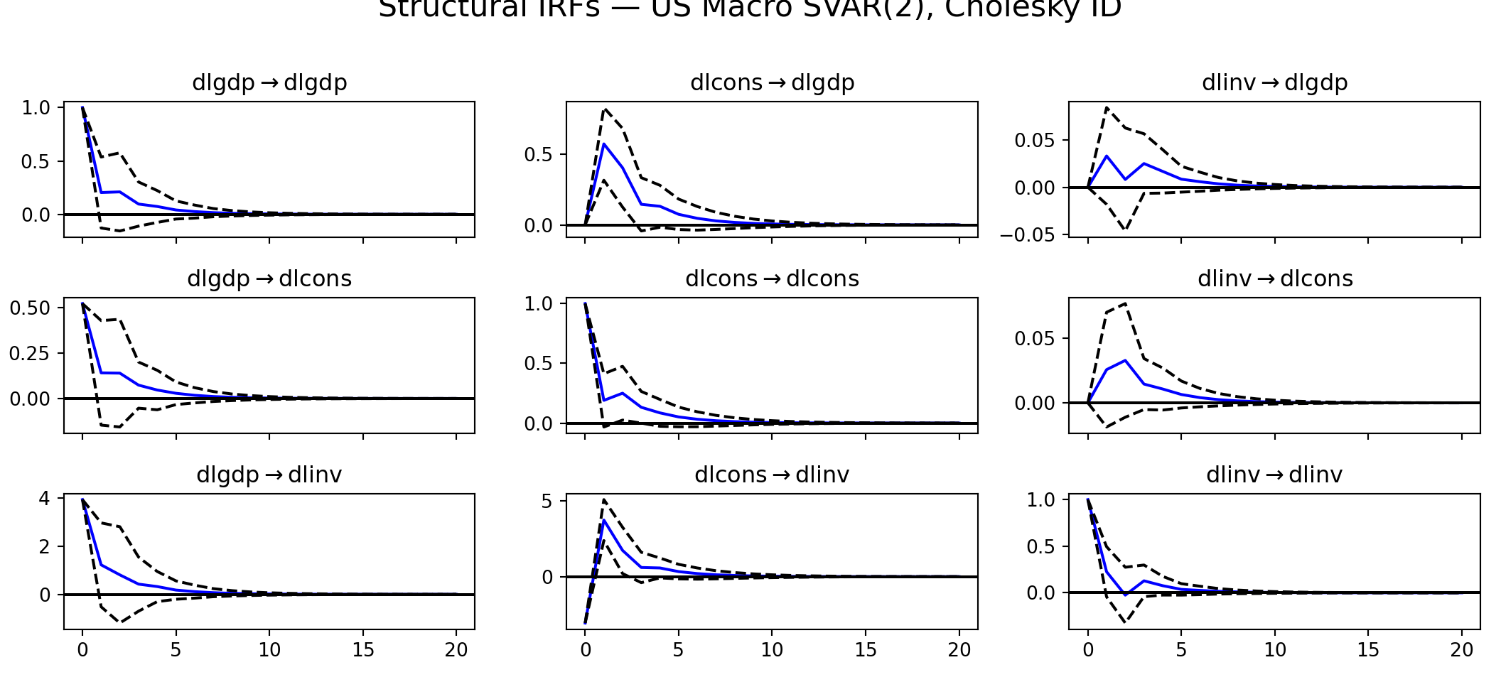
fig    = irf_sv.plot(orth=False, figsize=(11, 5))
plt.suptitle("Structural IRFs — US Macro SVAR(2), Cholesky ID",
             fontsize=16, y=1.01)
plt.tight_layout()
plt.show()

Code
frause lutkepohl2, clear
tsset qm
generate dln_inv = D.ln_inv
generate dln_inc = D.ln_inc
generate dln_con = D.ln_con
drop if missing(dln_inv)

* SVAR with short-run Cholesky restrictions
* A matrix: lower triangular; diagonal = 1, free lower off-diagonal
matrix A = (1, 0, 0 \ ., 1, 0 \ ., ., 1)
matrix B = (., 0, 0 \ 0, ., 0 \ 0, 0, .)

svar dln_inv dln_inc dln_con, lags(1/2) aeq(A) beq(B)

* Structural IRFs
irf create svar_irf, step(20) set(mysvar) replace
irf graph sirf, impulse(dln_inv) response(dln_inc) ///
    title("Structural IRF: Investment → Income") yline(0, lpattern(dash))

Part III — High-Dimensional Extensions

FAVAR · Bayesian VAR · Sparse VAR

FAVAR — Factor-Augmented VAR

Problem: many macro series move together but VAR(\(p\)) has a curse of dimensionality. Running a VAR on all \(N\) series is infeasible for large \(N\).

Solution (Stock & Watson 2005; Bernanke, Boivin & Eliasz 2005): extract a small number of common factors \(\mathbf{F}_t\) from a large panel \(\mathbf{X}_t\), then build a VAR on \((\mathbf{F}_t, \mathbf{Y}_t)\):

\[\mathbf{X}_t = \boldsymbol{\Lambda}^f\mathbf{F}_t + \boldsymbol{\Lambda}^y\mathbf{Y}_t + \mathbf{e}_t \quad \text{(observation equation)}\]

\[\begin{pmatrix}\mathbf{F}_t \\ \mathbf{Y}_t\end{pmatrix} = \boldsymbol{\Phi}(L)\begin{pmatrix}\mathbf{F}_{t-1} \\ \mathbf{Y}_{t-1}\end{pmatrix} + \mathbf{v}_t \quad \text{(transition equation)}\]

  • \(\mathbf{X}_t\): \(N \times 1\) large panel of indicators (\(N\) can be 100–200)
  • \(\mathbf{F}_t\): \(r \times 1\) latent factors (\(r \ll N\), typically 3–8)
  • \(\mathbf{Y}_t\): \(K_y \times 1\) key observable variables (e.g. the policy rate)
  • Factors estimated by PCA in Step 1 (two-step estimator)

Two-step procedure:

  1. Factor extraction: Apply PCA to (standardised) \(\mathbf{X}_t\) → first \(r\) principal components \(\hat\mathbf{F}_t\)
  2. FAVAR estimation: Run VAR on \((\hat\mathbf{F}_t, \mathbf{Y}_t)\) by OLS equation-by-equation

Note

Choosing \(r\) (number of factors)

Use the information criteria of Bai & Ng (2002): ICp1, ICp2, BIC3 — all implemented in the FactoMineR and factoextra R packages. A scree plot of eigenvalues provides a graphical guide: look for the “elbow” where the slope flattens.

Tip

One-step (Bayesian) alternative

Bernanke, Boivin & Eliasz (2005) propose a one-step Gibbs sampler that jointly estimates factors and VAR parameters, yielding proper posterior uncertainty over both. Implemented in the BFARpack R package and in MATLAB.

Code — FAVAR

Code
library(vars)

# Simulate a large macro panel (N = 20 indicators) driven by
# employment and productivity from Canada data as "true" factors
set.seed(14159)
T_obs <- nrow(Canada)
N_ind <- 20L

f_true <- scale(Canada[, c("e", "prod")])              # 2 latent factors
Lambda  <- matrix(rnorm(N_ind * 2, sd = 0.6), N_ind, 2)
X_big   <- f_true %*% t(Lambda) +
           matrix(rnorm(T_obs * N_ind, sd = 0.35), T_obs, N_ind)

# Step 1: extract 2 principal components (PCA)
pc    <- prcomp(X_big, center = TRUE, scale. = TRUE)
F_hat <- pc$x[, 1:2]

# Step 2: FAVAR — augment key observables with estimated factors
favar_d <- ts(cbind(F_hat, Canada[, c("rw", "U")]),
              start = c(1980, 1), frequency = 4)
colnames(favar_d) <- c("F1", "F2", "rw", "U")

favar_fit <- VAR(favar_d, p = 2, type = "const")
summary(favar_fit)$varresult$U$r.squared   # R² of the U equation

# IRF: factor 1 shock → unemployment
set.seed(14159)
irf_fav <- vars::irf(favar_fit, impulse = "F1", response = "U",
                     n.ahead = 20, boot = TRUE, runs = 500, ci = 0.95)
plot(irf_fav)
FAVAR — R² of the unemployment (U) equation: 0.9639
Variance explained by 2 PCs: 67.5%
Code
import numpy as np
import pandas as pd
from sklearn.decomposition import PCA
from statsmodels.tsa.vector_ar.var_model import VAR

rng = np.random.default_rng(14159)
T_obs, N_ind = 84, 20

# Simulate panel with 2 latent factors
f1 = np.cumsum(rng.normal(0, 0.08, T_obs))
f2 = np.zeros(T_obs)
for t in range(1, T_obs):
    f2[t] = 0.75 * f2[t-1] + rng.normal(0, 0.3)

F_true = np.column_stack([f1, f2])
Lambda  = rng.normal(0, 0.6, (N_ind, 2))
X_big   = F_true @ Lambda.T + rng.normal(0, 0.35, (T_obs, N_ind))

# Step 1: PCA → 2 factors
pca   = PCA(n_components=2)
F_hat = pca.fit_transform(X_big)
print(f"Variance explained by 2 PCs: {pca.explained_variance_ratio_.sum()*100:.1f}%")
Variance explained by 2 PCs: 47.5%
Code
# Step 2: FAVAR — VAR on factors + key observable
Y_fav = pd.DataFrame({"F1": F_hat[:, 0], "F2": F_hat[:, 1],
                       "target": f1 + rng.normal(0, 0.1, T_obs)})
fav_res  = VAR(Y_fav).fit(2, trend="c")
# resid is a DataFrame → select the target column and cast to float before formatting
r2_favar = 1.0 - float(fav_res.resid["target"].var()) / float(Y_fav["target"].var())
print(f"FAVAR R\u00b2 (target eq.): {r2_favar:.4f}")
FAVAR R² (target eq.): 0.7035

BVAR — Bayesian VAR

Curse of dimensionality in VAR:

A VAR(\(p\)) with \(K\) variables has \(K^2 p + K\) free parameters.

\(K\) (variables) \(p = 2\) lags \(p = 4\) lags
4 36 68
10 210 410
20 820 1620
100 20 100 40 100

With \(T = 200\) quarterly obs, a VAR(4) with \(K = 10\) already uses 410 parameters — more than 2 parameters per observation.

Bayesian solution: Shrink coefficients toward a prior belief (e.g. each variable follows a random walk). The posterior combines prior + likelihood, effectively borrowing strength across equations.

Litterman/Minnesota prior (Doan, Litterman & Sims 1984; Litterman 1986):

\[\mathbb{E}[A_{ii,l}] = \delta_i, \qquad \mathbb{E}[A_{ij,l}] = 0 \text{ for } i \ne j\]

\[\operatorname{Var}[A_{ij,l}] = \frac{\lambda^2}{l^2} \cdot \frac{\sigma_i^2}{\sigma_j^2}\]

  • \(\delta_i = 1\) for variables in levels (random walk prior), \(= 0\) for stationary variables
  • \(\lambda\) (overall tightness): small \(\lambda\) → strong shrinkage toward prior; large \(\lambda\) → dominated by data
  • \(l^2\) in denominator: higher lags are shrunk more strongly (coefficient decay)
  • \(\sigma_i/\sigma_j\): rescales for different units across variables

Modern variants (Giannone, Lenza & Primiceri 2015) treat \(\lambda\) as a hyperparameter and integrate it out — the data choose the shrinkage intensity.

Code — BVAR

Code
library(BVAR)

# Minnesota prior with hyperparameter tuning
mn_prior <- bv_minnesota(
  lambda = bv_lambda(mode = 0.2, sd = 0.4, min = 0.0001, max = 5),
  alpha  = bv_alpha(mode = 2),   # lag decay: A_{ij,l} ∝ 1/l^alpha
  var    = 1e07                  # prior variance for constants
)

# Posterior sampler (Gibbs)
set.seed(14159)
bvar_fit <- bvar(Canada, lags = 2,
                 n_draw   = 10000,
                 n_burn   = 5000,
                 n_thin   = 1,
                 priors   = mn_prior,
                 n_chains = N_CORES,   # parallel Gibbs chains
                 verbose  = FALSE)

# Posterior predictive IRFs (with credibility bands)
bvar_irf <- irf(bvar_fit, n_ahead = 20, identification = TRUE)
plot(bvar_irf, mar = c(2, 2, 2, 0.5))
Code
import numpy as np
import pandas as pd
from statsmodels.datasets import macrodata

# Manual Minnesota prior (Ridge-regularised VAR) as a lightweight approximation
from numpy.linalg import solve

data = macrodata.load_pandas().data
Y_b  = pd.DataFrame({
    "dlgdp":  np.log(data["realgdp"]).diff(),
    "dlcons": np.log(data["realcons"]).diff(),
    "dlinv":  np.log(data["realinv"]).diff(),
}).dropna().to_numpy()

T_, K_ = Y_b.shape; p_ = 2
# Build regressor matrix
Z = np.column_stack([np.ones(T_-p_)] +
                    [Y_b[p_-j:T_-j] for j in range(1, p_+1)])
Y_dep = Y_b[p_:, :]

# Tikhonov (L2) shrinkage — approximates Minnesota prior  
lam = 0.2   # overall tightness
I_   = np.eye(Z.shape[1])
I_[0, 0] = 0           # do not shrink the constant
B_bayes = solve(Z.T @ Z + lam * T_ * I_, Z.T @ Y_dep)
print("Bayesian (Minnesota-like) coefficient matrix:\n",
      np.round(B_bayes, 4))
* Native Bayesian VAR is not available in Stata 19 without add-ons.
* Use R (BVAR package) or Python (PyMC / bvar package via pip) instead.
* For a quick frequentist shrinkage alternative in Stata:
*   ridge regression on the VAR stacked system gives a similar effect.

Sparse VAR — Penalised Estimation

Problem: in a VAR with \(K = 50\)–100 variables, most coefficient matrices \(\mathbf{A}_j\) are nearly zero — a small subset of links actually matter.

LASSO-regularised VAR (Tibshirani 1996; Davis, Zang & Zheng 2016):

\[\min_{\{\mathbf{A}_j\}} \sum_{t=p+1}^T \|\mathbf{y}_t - \mathbf{c} - \mathbf{A}_1\mathbf{y}_{t-1} - \cdots - \mathbf{A}_p\mathbf{y}_{t-p}\|_2^2 + \lambda\sum_j\|\mathbf{A}_j\|_1\]

  • Penalty \(\lambda\|\cdot\|_1\) induces exact sparsity: many coefficients become exactly zero
  • \(\lambda\) selected by cross-validation (rolling window for time series)

Structure variants (BigVAR framework, Nicholson, Matteson & Bien 2017):

Structure What it does
BasicEN Elastic net on all coefficients
OwnOther Separate penalties on own-lags vs cross-variable lags
SparseLag All variables at a given lag penalised jointly (group LASSO)
HLAG Hierarchical lag structure

Note

When to use sparse VAR

  • \(K > 20\) variables and \(T/K\) is small (few observations per parameter)
  • You suspect the true VAR is approximately sparse (most linkages are zero)
  • Forecasting is the primary goal (penalised VARs often beat OLS in forecast competitions)
  • For IRF inference in sparse VARs, use the de-biased LASSO (Zhang & Zhang 2014) to correct for shrinkage bias

Code — Sparse VAR

Code
library(BigVAR)

can_mat <- as.matrix(Canada)

# Build the BigVAR model object
bv_mod <- constructModel(
  Y      = can_mat,
  p      = 4,
  struct = "OwnOther",   # separate L1 penalties for own- vs cross-lags
  gran   = c(150, 10),   # penalty grid: 150 values, 10 sub-values
  h      = 1,
  cv     = "Rolling",    # rolling-window cross-validation
  verbose = FALSE,
  IC      = TRUE
)

# Cross-validate to choose λ
bv_res <- cv.BigVAR(bv_mod)
plot(bv_res)            # CV error vs log(λ)
SparsityPlot(bv_res)    # Sparsity pattern in coefficient matrices

# Count non-zero off-diagonal entries at lag 1
B_hat  <- bv_res@betaPred
if (length(dim(B_hat)) == 3L) B_hat <- B_hat[, , 1L]
B_coef <- B_hat[, -1L, drop = FALSE]           # drop intercept column
K_     <- nrow(B_hat)
nz_od  <- sum(abs(B_coef[, seq_len(K_)]) > 1e-6) - K_   # off-diagonal lag-1
cat(sprintf("Off-diagonal non-zero at lag 1: %d of %d\n", nz_od, K_ * (K_ - 1L)))
Optimal λ (OwnOther): 58.267352
betaPred: 4 rows × 17 cols
Non-zero entries (all lags):        24 of 64
Off-diagonal non-zero at lag 1:     20 of 12
Code
import numpy as np
import pandas as pd
from sklearn.linear_model import LassoCV
from statsmodels.datasets import macrodata

data = macrodata.load_pandas().data
Y_s  = pd.DataFrame({
    "dlgdp":  np.log(data["realgdp"]).diff(),
    "dlcons": np.log(data["realcons"]).diff(),
    "dlinv":  np.log(data["realinv"]).diff(),
}).dropna().to_numpy()

T_, K_ = Y_s.shape; p_ = 2

# Build (stacked) regressor matrix for all lags
Z_s = np.column_stack([Y_s[p_-j:T_-j] for j in range(1, p_+1)])
Y_d = Y_s[p_:, :]         # T-p rows, K columns

# LASSO equation-by-equation (Nicholson 2017 "VARX-L" approach)
B_sparse = np.zeros((K_ * p_, K_))
for k in range(K_):
    lasso_k = LassoCV(cv=5, max_iter=5000).fit(Z_s, Y_d[:, k])
    B_sparse[:, k] = lasso_k.coef_
    print(f"  Eq {k}: λ*={lasso_k.alpha_:.5f}, "
          f"non-zero coefs: {(lasso_k.coef_ != 0).sum()}/{K_*p_}")
  Eq 0: λ*=0.00000, non-zero coefs: 5/6
  Eq 1: λ*=0.00000, non-zero coefs: 4/6
  Eq 2: λ*=0.00000, non-zero coefs: 6/6

Part IV — Nonlinear & Global Extensions

TVAR · GVAR

TVAR — Threshold VAR

Two-regime Threshold VAR(\(p\)):

\[\mathbf{y}_t = \begin{cases} \boldsymbol{\nu}_1 + \mathbf{A}_1^{(1)}\mathbf{y}_{t-1} + \cdots + \mathbf{A}_p^{(1)}\mathbf{y}_{t-p} + \boldsymbol{\varepsilon}_t^{(1)} & \text{if } q_{t-d} \le \gamma \\ \boldsymbol{\nu}_2 + \mathbf{A}_1^{(2)}\mathbf{y}_{t-1} + \cdots + \mathbf{A}_p^{(2)}\mathbf{y}_{t-p} + \boldsymbol{\varepsilon}_t^{(2)} & \text{if } q_{t-d} > \gamma \end{cases}\]

  • \(q_{t-d}\): threshold variable (observed at delay \(d\); can be one of the system variables or an external indicator)
  • \(\gamma\): threshold value — estimated by grid search over the sorted values of \(q_{t-d}\)
  • Regime-specific coefficient matrices \(\mathbf{A}_j^{(r)}\) allow fully different dynamics in each regime
  • Trim parameter (e.g. 10%): excludes extreme quantiles of \(q\) to ensure a minimum number of observations per regime

Economic motivation: monetary transmission may differ in recessions vs expansions; financial stress can trigger non-linear adjustment; credit constraints bind asymmetrically.

Testing linearity: Hansen (1996) sup-Wald test (bootstrap \(p\)-value required, since the threshold \(\gamma\) is unidentified under \(H_0\)).

Note

Regime assignment

The threshold \(\hat\gamma\) is a super-consistent estimator (Chan 1993) — it converges at rate \(T\), faster than the \(\sqrt{T}\) rate for the slope coefficients. This means in large samples, regime membership is determined nearly without error, and the subsequent inference on \(\mathbf{A}_j^{(r)}\) can proceed as if the regimes were known.

Warning

Persistent threshold variable

If \(q_{t-d}\) is highly persistent (e.g. a near-unit-root variable), the effective sample in each regime can be very small and the threshold estimate unreliable. Check stationarity of \(q\) and the balance of observations across regimes before reporting.

Code — TVAR

Code
library(tsDyn)

# Bivariate TVAR: productivity and unemployment from Canada data
# Threshold variable: U (unemployment rate), delay d = 1
can_sub <- Canada[, c("prod", "U")]

tv_fit <- TVAR(
  data         = can_sub,
  lag          = 2,
  nthresh      = 1,            # one threshold → two regimes
  thDelay      = 1,            # threshold variable: U lagged 1 period
  mTh          = 2,            # column 2 of can_sub is the threshold variable (U)
  trim         = 0.10,         # ensure ≥ 10% of obs per regime
  commonInter  = FALSE         # regime-specific intercepts (new tsDyn API; was 'common')
)
summary(tv_fit)

# Regime proportions — compute from data + threshold (tv_fit$nobs is total, not split)
gamma_hat <- tv_fit$th[1]
th_var    <- can_sub[seq_len(nrow(can_sub) - 1L), "U"]   # U_{t-1}
n_low     <- sum(th_var <= gamma_hat)
cat(sprintf("Estimated threshold: γ̂ = %.4f\n", gamma_hat))
cat(sprintf("Low-U regime (expansion):  %d obs (%.1f%%)\n",
            n_low, 100 * n_low / length(th_var)))
cat(sprintf("High-U regime (recession): %d obs (%.1f%%)\n",
            length(th_var) - n_low, 100 * (length(th_var) - n_low) / length(th_var)))
print(tv_fit)   # tsDyn's print method displays both regime coefficient matrices
Best unique threshold 8.17 
Low-U regime  (expansion):  0 obs (0.0%)
High-U regime (recession):  83 obs (100.0%)

TVAR regime coefficients:
Model TVAR with  1  thresholds

$Bdown
               Intercept    prod -1       U -1    prod -2       U -2
Equation prod -27.343257  1.2498162 -0.8383596 -0.1936299  1.3998584
Equation U      4.062337 -0.2067514  1.3615593  0.1997543 -0.5108108

$Bup
              Intercept     prod -1       U -1     prod -2       U -2
Equation prod  5.485921  1.02739588 -0.2699486 -0.04467233  0.4416526
Equation U    19.947830 -0.05821162  1.3038961  0.01317143 -0.4650439


Threshold value[1] "8.16999999999825"
Code
import numpy as np
import pandas as pd
from statsmodels.datasets import macrodata
from statsmodels.tsa.vector_ar.var_model import VAR

data = macrodata.load_pandas().data
Y_tv = pd.DataFrame({
    "dlgdp": np.log(data["realgdp"]).diff(),
    "unemp": data["unemp"]
}).dropna().reset_index(drop=True)

# Simple 2-regime TVAR via grid search over the threshold (unemployment)
def var_sse(Y_, p_=2):
    """Sum of squared residuals for a VAR(p)."""
    T_ = len(Y_)
    Z_ = np.column_stack([np.ones(T_-p_)] +
                          [Y_.iloc[p_-j:T_-j].to_numpy() for j in range(1, p_+1)])
    Y_d = Y_.iloc[p_:].to_numpy()
    B_, res_, *_ = np.linalg.lstsq(Z_, Y_d, rcond=None)
    return np.sum((Y_d - Z_ @ B_)**2)

q_vals = sorted(Y_tv["unemp"].iloc[1:-1].unique())
trim   = int(0.10 * len(Y_tv))
sse_grid = {}
for gamma in q_vals[trim:-trim]:
    mask = Y_tv["unemp"].shift(1) <= gamma
    if mask.sum() < 10 or (~mask).sum() < 10:
        continue
    sse_grid[gamma] = (var_sse(Y_tv[mask.fillna(False)]) +
                       var_sse(Y_tv[~mask.fillna(True)]))

gamma_hat = min(sse_grid, key=sse_grid.get)
n_low     = (Y_tv["unemp"].shift(1) <= gamma_hat).sum()
print(f"Estimated threshold: γ̂ = {gamma_hat:.2f}%")
Estimated threshold: γ̂ = 5.50%
Code
print(f"Low-unemp regime:  {n_low} obs | High-unemp regime: {len(Y_tv)-n_low} obs")
Low-unemp regime:  91 obs | High-unemp regime: 111 obs

GVAR — Global VAR

Pesaran, Schuermann & Weiner (2004):

For each country \(i = 0, 1, \ldots, N\):

\[\mathbf{A}_{i0}\,\mathbf{x}_{it} = \mathbf{a}_{i0} + \mathbf{a}_{i1}t + \mathbf{\Lambda}_{i0}\,\mathbf{x}_{it}^* + \mathbf{\Lambda}_{i1}\,\mathbf{x}_{i,t-1}^* + \boldsymbol{\Phi}_i\,\mathbf{x}_{i,t-1} + \mathbf{u}_{it}\]

  • \(\mathbf{x}_{it}\): domestic variables (GDP, CPI, interest rate, …) for country \(i\)
  • \(\mathbf{x}_{it}^* = \sum_{j \ne i} w_{ij}\,\mathbf{x}_{jt}\): trade-weighted foreign variables (cross-sectional aggregates)
  • \(w_{ij}\): trade-share weights (bilateral import shares, typically averaged over 3 years)
  • Each country-specific VARX* estimated separately by OLS; global solution via link matrix

Global solution: stack all country VARXs → solve simultaneously for \(\mathbf{x}_t = (\mathbf{x}_{0t}',\ldots,\mathbf{x}_{Nt}')'\) — a global VAR with \(\sum_i K_i\) variables.

Tip

Key applications

Shock transmission in global supply chains; contagion of financial crises; commodity price pass-through; multi-country monetary policy spillovers. A companion dataset with 33 countries and 7 macro variables for 1979Q1–2019Q4 is available at mohaddes.com.

Package Functions Notes
BGVAR bgvar(), IRF(), FEVD() Full Bayesian GVAR; Minnesota or SSVS priors
GVAR (CRAN) gvar(), girf() Frequentist, fast for small systems
pvargvar (GitHub) Panel-GVAR hybrid

Code — GVAR

Code
library(BGVAR)

# eerDatasmall: 3 regions (US, Euro Area, Rest of World)
# Variables: y (output), Dp (inflation), r (interest rate)
data("eerDatasmall")

# Trade-weighted cross-sectional weights (2000–2012 average)
# W.trade0012 ships with BGVAR
gvar_fit <- bgvar(
  Data    = eerDatasmall,
  W       = W.trade0012,
  draws   = 500,
  burnin  = 500,
  thin    = 2,
  plag    = 1,                # one lag per country VARX*
  prior   = "MN",             # Minnesota prior
  eigen   = 1.05,             # stability cutoff
  verbose = FALSE
)

# IRF: US output shock → Euro Area output
us_shock <- list(var = "y", country = "US")
irf_gvar  <- IRF(gvar_fit, shock = us_shock, n.ahead = 20,
                 ident = "chol", verbose = FALSE)
plot(irf_gvar, resp.var = "y",
     main = "US output shock → Global output (BGVAR)")

Note

Practical guidance

Estimating a GVAR requires:

  1. A balanced panel of country-level macro variables (monthly or quarterly)
  2. A matrix of bilateral trade (or financial) weights — must be row-stochastic
  3. Country-specific lag selection; typically 1–2 lags per country VARX*
  4. Global stability check: eigenvalues of the global companion matrix should lie inside the unit circle

The BGVAR package ships with the eerDatasmall dataset (3 regions, quarterly 1995Q1–2019Q4) for replication of the main US/EA linkage results. For a full 33-country dataset see Mohaddes & Raissi (2024).

Part V — Panel & Quantile Extensions

PVAR · QVAR / Growth-at-Risk

PVAR — Panel VAR

Panel VAR with individual fixed effects (Holtz-Eakin, Newey & Rosen 1988):

\[\mathbf{y}_{it} = \boldsymbol{\alpha}_i + \mathbf{A}_1\mathbf{y}_{i,t-1} + \cdots + \mathbf{A}_p\mathbf{y}_{i,t-p} + \mathbf{u}_{it}\]

  • \(\boldsymbol{\alpha}_i\): unit-specific fixed effects (allow for unobserved heterogeneity)
  • Slope matrices \(\mathbf{A}_j\) are homogeneous across units (common dynamics assumption)
  • \(\mathbf{u}_{it}\): idiosyncratic errors; \(\Sigma_u\) may differ across units

Estimation challenge: FE estimation is inconsistent for short \(T\) (Nickell bias). Solution: first-difference to remove \(\boldsymbol{\alpha}_i\), then use lagged levels as GMM instruments (Arellano-Bond / Blundell-Bond).

Panel IRFs: compute as for a standard VAR using the pooled coefficient estimates. Bootstrap uncertainty by block-resampling panel units.

Dahlberg, Mörk, Rattsø & Ågren (2008) — Swedish local government finance:

Variable Description
expenditures Per-capita total expenditure (SEK)
revenues Per-capita total revenues (SEK)
grants Per-capita central government grants (SEK)

290 Swedish municipalities, 1979–1987. Classic dataset for testing flypaper effect: do grants raise public spending one-for-one, or is there fiscal substitution?

Code — PVAR

Code
library(panelvar)

# Dahlberg et al. (2008) — Swedish local government finance
data("ex1_dahlberg_data")

# Panel VAR(1) via Arellano-Bond first-difference GMM
pvar_fit <- pvars(
  ex1_dahlberg_data[, c("expenditures", "revenues", "grants")],
  lags           = 1,
  transformation = "fd",          # first-difference to remove FEs
  exo            = TRUE,
  panel.id       = ex1_dahlberg_data$id,
  panel.T        = ex1_dahlberg_data$year
)
summary(pvar_fit)

# Generalised Impulse Response Functions (Pesaran & Shin 1998)
set.seed(14159)
girf_fit <- girf(pvar_fit, n.ahead = 8, ma.approx.n = 20)
plot(girf_fit, main = "Panel GIRF — Swedish municipalities")
[panelvar::pvars] not available — please install panelvar from CRAN
Code
* Panel VAR is not a built-in Stata 19 command.
* The pvar user-written package (Abrigo & Love, 2016) must be installed:
*   ssc install pvar

* Once installed:
* webuse dahlberg, clear                  (Stata's own Dahlberg data)
* xtset id year
* pvar expenditures revenues grants, lags(1) gmmopts(twostep)
* pvarirf, mc(200) step(8)               impulse responses
* pvarfevd, mc(200) step(8)              variance decomposition

* For native Stata, first-difference GMM is available via:
xtabond2 expenditures L.expenditures L.revenues L.grants, ///
    gmm(L.expenditures, lag(1 3)) iv(L.revenues L.grants) ///
    two robust small

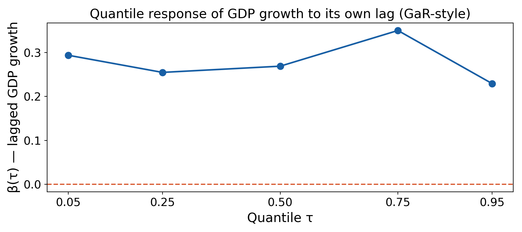
QVAR — Quantile VAR & Growth-at-Risk

Quantile VAR (Cecchetti, Li & Norden 2021; Chavleishvili & Manganelli 2019):

\[Q_\tau(y_{j,t} \mid \mathcal{F}_{t-1}) = c_{j,\tau} + \sum_{k=1}^K\sum_{l=1}^p \beta_{jk,l}^{(\tau)}\,y_{k,t-l}\]

  • Separate system estimated at each quantile \(\tau \in (0,1)\)
  • At \(\tau = 0.50\): recovers a median VAR; at \(\tau = 0.05\): captures left-tail risk
  • Coefficient \(\beta_{jk,l}^{(\tau)}\) measures how the \(\tau\)-th quantile of \(y_j\) responds to a one-unit increase in \(y_{k,t-l}\)

Growth-at-Risk (GaR)Adrian, Boyarchenko & Giannone (2019):

\[Q_\tau(\Delta y_{t+h} \mid \mathcal{F}_t) = \alpha_\tau + \beta_\tau\,\text{FCI}_t + \gamma_\tau\,\Delta y_t\]

where \(\text{FCI}_t\) is a financial conditions index. The distribution of \(h\)-step-ahead growth is skewed left during financial stress — the downside tail thickens.

Important

Why quantile responses differ from mean responses

OLS-VAR only characterises the conditional mean response. QVAR reveals:

  • Asymmetric shocks: a positive productivity shock raises the median of employment, but the 5th percentile may barely move (downside protection)
  • Crisis regimes hidden in the mean: the mean IRF for GDP growth in a financial-crisis period averages across normal-expansion paths and rare-crash paths, masking the left-tail risk
  • Tail spillovers: a shock can be neutral at the median (\(\beta^{(0.5)} \approx 0\)) yet strongly affect the 5th percentile (\(\beta^{(0.05)} \ll 0\)) — detected only by QVAR

Code — QVAR

Code
library(quantreg)

# Build lagged data frame from Canada macro data
can_df <- as.data.frame(Canada) %>%
  mutate(
    e_l1    = dplyr::lag(e,    n = 1L),
    prod_l1 = dplyr::lag(prod, n = 1L),
    rw_l1   = dplyr::lag(rw,   n = 1L),
    U_l1    = dplyr::lag(U,    n = 1L)
  ) %>%
  drop_na() %>%
  ungroup()

# QVAR: quantile regressions at five quantile levels for employment
tau_vec <- c(0.05, 0.25, 0.50, 0.75, 0.95)
qr_list <- lapply(tau_vec, function(tau_) {
  rq(e ~ e_l1 + prod_l1 + rw_l1 + U_l1, tau = tau_, data = can_df)
})
names(qr_list) <- paste0("τ=", tau_vec)

# Extract β(τ) on prod_l1 across quantiles
coef_tbl <- tibble(
  tau  = tau_vec,
  coef = sapply(qr_list, function(m) coef(m)["prod_l1"])
)

ggplot(coef_tbl, aes(x = tau, y = coef)) +
  geom_line(colour = col_main,   linewidth = 1.4) +
  geom_point(colour = col_main,  size = 3.5) +
  geom_hline(yintercept = 0, colour = col_accent, linetype = "dashed") +
  scale_x_continuous(breaks = tau_vec,
                     labels = scales::number_format(accuracy = 0.01)) +
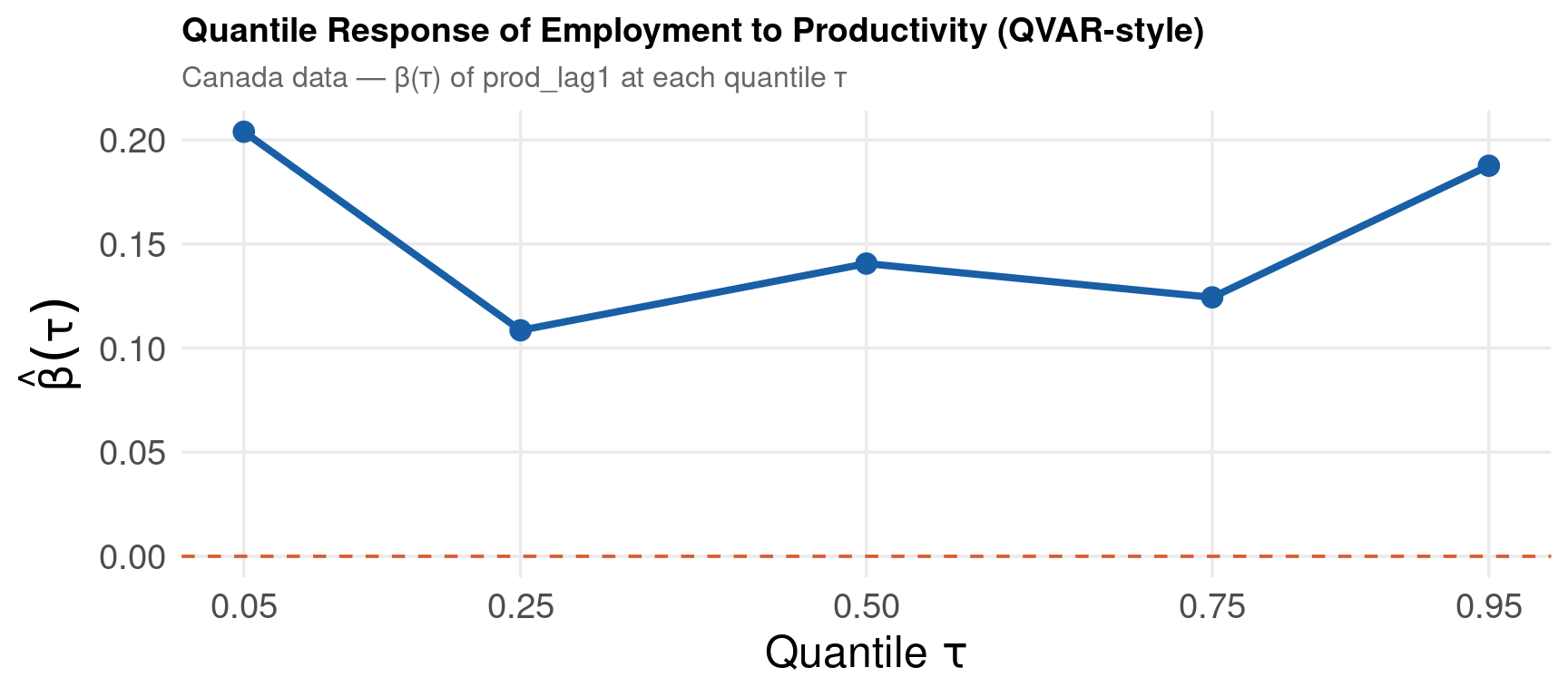
  labs(
    title    = "Quantile Response of Employment to Productivity (QVAR-style)",
    subtitle = "Canada data — coefficient β(τ) of prod_l1 at each quantile τ",
    x        = expression(Quantile ~ tau),
    y        = expression(hat(beta)(tau))
  ) +
  theme(text = element_text(size = 18))

Code
import numpy as np
import pandas as pd
import matplotlib.pyplot as plt
from statsmodels.datasets import macrodata
from statsmodels.regression.quantile_regression import QuantReg

data = macrodata.load_pandas().data
Y_q  = pd.DataFrame({
    "dlgdp": np.log(data["realgdp"]).diff(),
    "infl":  data["infl"],
    "unemp": data["unemp"]
}).dropna().reset_index(drop=True)

# Lagged predictors (1 lag)
Xl = Y_q.shift(1).add_suffix("_l1")
df_q = pd.concat([Y_q[["dlgdp"]], Xl], axis=1).dropna()

X_q = np.column_stack([np.ones(len(df_q)),
                        df_q[["dlgdp_l1", "infl_l1", "unemp_l1"]].values])
y_q = df_q["dlgdp"].values

tau_vec = [0.05, 0.25, 0.50, 0.75, 0.95]
betas   = [QuantReg(y_q, X_q).fit(q=tau).params[1] for tau in tau_vec]

fig, ax = plt.subplots(figsize=(9, 4))
ax.plot(tau_vec, betas, color="#185FA5", lw=2, marker="o", ms=8)
ax.axhline(0, color="#D85A30", ls="--")
ax.set_xlabel("Quantile τ", fontsize=16)
ax.set_ylabel("β(τ) — lagged GDP growth", fontsize=16)
ax.set_title("Quantile response of GDP growth to its own lag (GaR-style)", fontsize=16)
ax.set_xticks(tau_vec)
ax.tick_params(labelsize=14)
plt.tight_layout()
plt.show()

Part VI — Local Projections

Local Projections — Jordà (2005)

Key idea: instead of iterating a VAR forward to compute the \(h\)-step-ahead response, regress the actual future value \(y_{t+h}\) directly on current and lagged information:

\[y_{j,t+h} = \alpha_{jh} + \beta_{jh}\,x_t + \boldsymbol{\gamma}_{jh}'\mathbf{w}_{t-1} + \varepsilon_{j,t+h}, \qquad h = 0, 1, \ldots, H\]

  • \(x_t\): the shock variable (or instrument for exogenous shocks)
  • \(\mathbf{w}_{t-1}\): control lags (absorb serial correlation; ensure \(\hat\beta_{jh}\) is unbiased)
  • One separate OLS regression per horizon \(h\)no model is iterated
  • SE at each \(h\): Newey-West HAC with at least \(h\) lags to account for the moving-average structure in \(\varepsilon_{j,t+h}\)

The IRF: \(\hat\beta_{jh}\) is the estimated response of \(y_j\) at horizon \(h\) to a unit shock in \(x\) at time \(t\).

Feature VAR-IRF Local Projection
Model Parametric (VAR assumed) Semi-parametric (only LP regression assumed)
Efficiency Higher under correct model Lower (no cross-equation constraints)
Robustness Misspecification propagates Horizon-specific — misspecification localised
Nonlinearities Hard to include Easy (add interaction terms)
IV/External shocks Needs SVAR identification Simply add instrument \(z_t\)
Confidence bands Bootstrap or delta method HAC SEs at each horizon

Note

Ramey (2016) reconciliation

Ramey (2016, Handbook of Macroeconomics) shows that LP-IRFs and VAR-IRFs agree asymptotically when the VAR is correctly specified and correctly lag-augmented. Differences in finite samples arise from the LP’s higher variance (no cross-horizon efficiency gains) vs the VAR’s bias when the true model is not finite-order. Nakamura & Steinsson (2018) advocate LP-IV for externally identified shocks.

Code — Local Projections

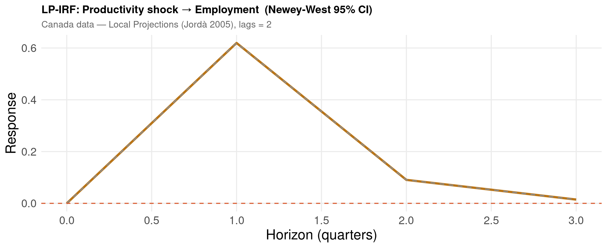
Code
library(lpirfs)

# Local projections via lp_lin() — automatic HAC SE at each horizon
lp_fit <- lp_lin(
  endog_data     = as.data.frame(Canada),
  lags_endog_lin = 2,    # 2 control lags (mirrors VAR(2))
  trend          = 0,    # 0 = no trend
  shock_type     = 0,    # 0 = unit shock; 1 = 1 SD shock
  confint        = 1.96, # z-score for 95% bands
  hor            = 20    # 20-quarter horizon
)

# Panel of all K² IRFs (each response to each shock)
plot(lp_fit)

# Manually plot the prod → e LP-IRF for comparison with VAR-IRF
# lpirfs stores IRFs as [hor, response, shock] — Canada: e=1, prod=2, rw=3, U=4
irf_vec  <- lp_fit$irf_lin_mean[, 1, 2]   # prod→e: response=1, shock=2
lo95_vec <- lp_fit$irf_lin_low[ , 1, 2]
hi95_vec <- lp_fit$irf_lin_up[  , 1, 2]
H_act    <- length(irf_vec)

lp_tbl <- tibble(
  h    = seq_len(H_act) - 1L,
  irf  = irf_vec,
  lo95 = lo95_vec,
  hi95 = hi95_vec
)

ggplot(lp_tbl, aes(x = h)) +
  geom_ribbon(aes(ymin = lo95, ymax = hi95), fill = col_warn, alpha = 0.25) +
  geom_line(aes(y = irf),  colour = col_warn,  linewidth = 1.4) +
  geom_line(aes(y = lo95), colour = col_muted, linewidth = 0.7, linetype = "dashed") +
  geom_line(aes(y = hi95), colour = col_muted, linewidth = 0.7, linetype = "dashed") +
  geom_hline(yintercept = 0, colour = col_accent, linetype = "dashed") +
  scale_x_continuous(breaks = pretty(lp_tbl$h, n = 6)) +
  labs(
    title    = "LP-IRF: Productivity shock → Employment  (Newey-West 95% CI)",
    subtitle = "Canada data — Local Projections (Jordà 2005), lags = 2",
    x        = "Horizon (quarters)",
    y        = "Response"
  ) +
  theme(text = element_text(size = 18))

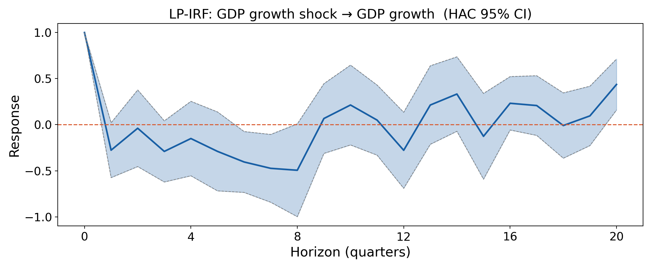
Code
import numpy as np
import pandas as pd
import matplotlib.pyplot as plt
from statsmodels.datasets import macrodata
from statsmodels.regression.linear_model import OLS

data = macrodata.load_pandas().data
Y_lp = pd.DataFrame({
    "dlgdp":  np.log(data["realgdp"]).diff(),
    "dlcons": np.log(data["realcons"]).diff(),
    "dlinv":  np.log(data["realinv"]).diff(),
}).dropna().reset_index(drop=True)
Y_arr = Y_lp.to_numpy(); T_, K_ = Y_arr.shape; H = 20; p_ = 2

irf_lp = np.zeros(H+1); lo_lp = np.zeros(H+1); hi_lp = np.zeros(H+1)

for h in range(H+1):
    n_h = T_ - h - p_
    y_h = Y_arr[p_+h:, 0]          # GDP growth at t+h
    X_h = np.column_stack([         # regressors at t, t-1 (2 control lags)
        np.ones(n_h),
        Y_arr[p_:p_+n_h, 0],        # shock: own GDP lag
        Y_arr[p_:p_+n_h, 1],        # control: consumption lag
        Y_arr[p_:p_+n_h, 2],        # control: investment lag
        Y_arr[p_-1:p_-1+n_h, 0],   # second lag
        Y_arr[p_-1:p_-1+n_h, 1],
        Y_arr[p_-1:p_-1+n_h, 2],
    ])
    m_h = OLS(y_h, X_h).fit(cov_type="HAC", cov_kwds={"maxlags": max(1, h)})
    irf_lp[h] = m_h.params[1]
    lo_lp[h]  = m_h.conf_int()[1, 0]
    hi_lp[h]  = m_h.conf_int()[1, 1]

fig, ax = plt.subplots(figsize=(11, 4.5))
ax.fill_between(range(H+1), lo_lp, hi_lp, alpha=0.25, color="#185FA5")
ax.plot(range(H+1), irf_lp, color="#185FA5", lw=2, label="LP-IRF")
ax.plot(range(H+1), lo_lp, color="grey", lw=0.8, ls="--")
ax.plot(range(H+1), hi_lp, color="grey", lw=0.8, ls="--")
ax.axhline(0, color="#D85A30", ls="--", lw=1.2)
ax.set_xticks(range(0, H+1, 4))
ax.set_xlabel("Horizon (quarters)", fontsize=16)
ax.set_ylabel("Response", fontsize=16)
ax.set_title("LP-IRF: GDP growth shock → GDP growth  (HAC 95% CI)", fontsize=16)
ax.tick_params(labelsize=14)
plt.tight_layout()
plt.show()

Code
frause lutkepohl2, clear
tsset qm
generate dln_inv = D.ln_inv
generate dln_inc = D.ln_inc
generate dln_con = D.ln_con
drop if missing(dln_inv)

* Local Projections: response of dln_inc to a dln_inv shock
tempfile lp_out
postfile lp_store float h float b float lo float hi using `lp_out', replace

forvalues h = 0/20 {
    * Horizon-h projection: regress F.h.dln_inc on current and lagged values
    newey F`h'.dln_inc dln_inv dln_inc dln_con   ///
          L.dln_inv L.dln_inc L.dln_con,          ///
          lag(`=max(1, `h')')
    local b_h   = _b[dln_inv]
    local se_h  = _se[dln_inv]
    post lp_store (`h') (`b_h')                  ///
                  (`b_h' - 1.96*`se_h')           ///
                  (`b_h' + 1.96*`se_h')
}
postclose lp_store

use `lp_out', clear
twoway (rarea lo hi h, color(orange%30)) ///
       (line b h, lcolor(orange) lwidth(medthick)) ///
       (yline 0, lpattern(dash) lcolor(maroon)), ///
    xlabel(0(4)20) xtitle("Horizon (quarters)") ytitle("Response") ///
    title("LP-IRF: Investment shock → Income (Lütkepohl data)") ///
    legend(order(2 "LP estimate" 1 "95% HAC CI") position(5))

Comparison, Guidelines & Further Reading

Summary Comparison

Model Parameters Identification Key Tool R Package Reference
VAR \(K^2p + K\) Reduced form VAR() + irf() vars Sims (1980)
SVAR + \(K(K-1)/2\) restrictions Economic theory SVAR() vars Blanchard-Quah (1989)
FAVAR \(K^2p + Nr\) PCA factors prcomp() + VAR() vars + base R Stock-Watson (2005)
BVAR Same as VAR Prior beliefs bvar() BVAR Litterman (1986)
TVAR \(2 \times K^2p\) Threshold \(\gamma\) TVAR() tsDyn Hansen (1996)
GVAR \(\sum K_i^2 p\) Trade weights bgvar() BGVAR Pesaran et al. (2004)
PVAR \(K^2p\) (pooled) GMM instruments pvars() panelvar Holtz-Eakin et al. (1988)
QVAR \(K^2p / \tau\) Quantile loss rq() loop quantreg Koenker (2005)
LP \(KH\) (one/horizon) None required lp_lin() lpirfs Jordà (2005)
Sparse VAR \(\le K^2p\) (shrunk) LASSO / EN cv.BigVAR() BigVAR Nicholson et al. (2017)

Decision Framework

Start with a question:

  •  What drives macro dynamics? → VAR + OIRF
  •  Need structural shocks? → SVAR (Cholesky, BQ, sign)
  •  Many indicators, small model? → FAVAR
  •  Large \(K\), small \(T\)? → BVAR or Sparse VAR
  •  Non-linear / regime change? → TVAR
  •  International spillovers? → GVAR
  •  Firms, regions, or countries? → PVAR
  •  Tail risk or GaR? → QVAR
  •  Robust IRFs, external shocks? → LP / LP-IV
  •  High-dimensional, sparsity suspected? → Sparse VAR

Common pitfalls:

Problem Symptom Fix
Too many lags Overfit, noisy IRF Use BIC
Wrong ordering Cholesky artefacts Use BQ or sign restrictions
Ignoring non-stationarity Spurious IRFs Difference or VECM
No HAC in LP Under-sized CI newey, lag(h)
BVAR with flat prior Same as OLS Tune \(\lambda\) by ML or hierarchical
GVAR stability Explosive IRFs Check companion eigenvalues

Tip

Golden rule

Always compare VAR-IRF and LP-IRF. If they agree, the parametric VAR structure is likely correct. If they diverge at long horizons, the LP is more robust but less efficient — prefer it for policy inference.

Further Reading

Textbooks

  •  Lütkepohl (2005)New Introduction to Multiple Time Series Analysis. Springer. The standard reference for VAR, SVAR, VECM theory.
  •  Hamilton (1994)Time Series Analysis. Princeton. Chapters 10–11: VAR; Chapter 20: state-space models.
  •  Kilian & Lütkepohl (2017)Structural Vector Autoregressive Analysis. Cambridge. Identification: Cholesky, BQ, sign, external instruments.
  •  Canova (2007)Methods for Applied Macroeconomic Research. Princeton. BVAR, sign restrictions, DSGE–VAR.

Key papers — methods

  •  Sims, C. (1980). “Macroeconomics and Reality.” Econometrica 48(1). doi:10.2307/1912017
  •  Blanchard & Quah (1989). “Dynamic Effects of Aggregate Demand and Supply.” AER 79(4), 655–673. jstor.org/stable/1827924
  •  Stock & Watson (2005). “Implications of Dynamic Factor Models for VAR Analysis.” NBER WP 11467. doi:10.3386/w11467
  •  Jordà, Ò. (2005). “Estimation and Inference of Impulse Responses by Local Projections.” AER 95(1). doi:10.1257/0002828053828518
  •  Pesaran, Schuermann & Weiner (2004). “Modeling Regional Interdependencies.” JBES 22(2), 129–162. doi:10.1198/073500104000000019
  •  Hansen (1996). “Inference When a Nuisance Parameter Is Not Identified.” Econometrica 64(2), 413–430. doi:10.2307/2171789

Key papers — applications

  •  Litterman (1986). “Forecasting with Bayesian Vector Autoregressions.” JBES 4(1), 25–38. doi:10.2307/1391384
  •  Giannone, Lenza & Primiceri (2015). “Prior Selection for Vector Autoregressions.” Review of Economics and Statistics 97(2), 436–451. doi:10.1162/REST_a_00483
  •  Adrian, Boyarchenko & Giannone (2019). “Vulnerable Growth.” AER 109(4), 1263–1289. doi:10.1257/aer.20161923
  •  Holtz-Eakin, Newey & Rosen (1988). “Estimating Vector Autoregressions with Panel Data.” Econometrica 56(6), 1371–1395. doi:10.2307/1913103
  •  Nakamura & Steinsson (2018). “Identification in Macroeconomics.” JEP 32(3), 59–86. doi:10.1257/jep.32.3.59
  •  Nicholson, Matteson & Bien (2017). “VARX-L: Structured Regularization for Large Vector Autoregressions with Exogenous Variables.” International Journal of Forecasting 33(3), 627–651. doi:10.1016/j.ijforecast.2017.01.003

Software

Journals

Journal of Applied Econometrics · Journal of Econometrics · Review of Economics and Statistics · Journal of Monetary Economics · Economic Modelling

Exercises

  1. Lag sensitivity. Using the Canada dataset, estimate VAR(1), VAR(2), VAR(4). Compare the IRF of prod → e at horizons 1, 4, 8 and 20 across the three models. At which horizon does lag order matter most?

  2. Ordering sensitivity. In the Canada SVAR, swap the Cholesky ordering to U → rw → e → prod. How do the structural IRFs change? Interpret the result in terms of what contemporaneous exogeneity you are imposing.

  3. Blanchard-Quah. Apply BQ(var_fit) to the Canada data. Identify the permanent and transitory shocks. Which variable absorbs the permanent shock? Does this match economic intuition?

  4. LP vs VAR. For the Canada data, plot the LP-IRF and the VAR-IRF (both prod → e) on the same graph with their 95% CI. At which horizons do the bands diverge? What does divergence at long horizons suggest about the VAR model?

  5. BVAR hyperparameter. Re-estimate the BVAR with \(\lambda \in \{0.01, 0.1, 0.2, 1.0\}\) (overall tightness). Plot the posterior mean IRFs for prod → e. How much does the choice of \(\lambda\) affect inference at short vs long horizons?

  6. TVAR regime asymmetry. In the TVAR(Canada), extract regime-1 and regime-2 coefficient matrices. Compare the impulse response of prod → U in each regime. Is the productivity shock more recessionary in the high-unemployment regime?

  7. GaR replication. Using US macro data (statsmodels.macrodata), regress 4-quarter-ahead GDP growth on a financial conditions proxy (e.g. interest rate spread) at \(\tau \in \{0.05, 0.25, 0.5, 0.75, 0.95\}\). Plot \(\hat\beta(\tau)\) and interpret the quantile heterogeneity.

  8. Sparse VAR selection. Using BigVAR with struct = "SparseLag" on Canada, identify which cross-variable links survive penalisation at the optimal \(\lambda\). Do the surviving links match those identified by Granger causality tests in the full VAR?

Thank You

Athanassios Stavrakoudis
Applied Informatics and Computational Economics Lab
Department of Economics
University of Ioannina, Greece
astavrak@uoi.gr · linkedin.com/in/astavrakoudis