2 Accessing Eurostat Database with API
2.1 SDMX with R
Eurostat is part of the SDMX consortium and redistributes data in SDMX format. All Eurostat tables can be found from : hhtp://ec.europa.eu/eurostat/SDMX/diss-web/rest/data/table_name
For exaxmple: http://ec.europa.eu/eurostat/SDMX/diss-web/rest/data/tin00028 has the data about internet usage by individuals.
Easy to download like this:
library(tidyverse)
library(rsdmx)

url  <- "http://ec.europa.eu/eurostat/SDMX/diss-web/rest/data/tin00028"
sdmx <- readSDMX(url)
as_tibble(sdmx)
## # A tibble: 2,112 × 9
## UNIT INDIC_IS IND_TYPE GEO FREQ obsTime obsValue OBS_STATUS OBS_FLAG
## <chr> <chr> <chr> <chr> <chr> <chr> <dbl> <chr> <chr>
## 1 PC_IND I_ILT12 IND_TOTAL AL A 2010 NA na <NA>
## 2 PC_IND I_ILT12 IND_TOTAL AL A 2011 NA na <NA>
## 3 PC_IND I_ILT12 IND_TOTAL AL A 2012 NA na <NA>
## 4 PC_IND I_ILT12 IND_TOTAL AL A 2013 NA na <NA>
## 5 PC_IND I_ILT12 IND_TOTAL AL A 2014 NA na <NA>
## 6 PC_IND I_ILT12 IND_TOTAL AL A 2015 NA na <NA>
## 7 PC_IND I_ILT12 IND_TOTAL AL A 2016 NA na <NA>
## 8 PC_IND I_ILT12 IND_TOTAL AL A 2017 NA na <NA>
## 9 PC_IND I_ILT12 IND_TOTAL AL A 2018 65 <NA> <NA>
## 10 PC_IND I_ILT12 IND_TOTAL AL A 2019 70 <NA> <NA>
## # … with 2,102 more rowsconversion from XML to data frame can be made also with:
However here we prefer to tidy approach with as_tibble.
The user can identify period of interest to limit data in specific periods of time. In this example this not a problem, but in larger datasets this might be useful. Here is how we can request data for specific time periods:
url  <- "http://ec.europa.eu/eurostat/SDMX/diss-web/rest/data/tin00028/all/?startperiod=2013&endPeriod=2018"
sdmx <- readSDMX(url)
as_tibble(sdmx)
## # A tibble: 1,056 × 9
## UNIT INDIC_IS IND_TYPE GEO FREQ obsTime obsValue OBS_STATUS OBS_FLAG
## <chr> <chr> <chr> <chr> <chr> <chr> <dbl> <chr> <chr>
## 1 PC_IND I_ILT12 IND_TOTAL AL A 2013 NA na <NA>
## 2 PC_IND I_ILT12 IND_TOTAL AL A 2014 NA na <NA>
## 3 PC_IND I_ILT12 IND_TOTAL AL A 2015 NA na <NA>
## 4 PC_IND I_ILT12 IND_TOTAL AL A 2016 NA na <NA>
## 5 PC_IND I_ILT12 IND_TOTAL AL A 2017 NA na <NA>
## 6 PC_IND I_ILT12 IND_TOTAL AL A 2018 65 <NA> <NA>
## 7 PC_IND I_ILT12 IND_TOTAL AT A 2013 82 <NA> <NA>
## 8 PC_IND I_ILT12 IND_TOTAL AT A 2014 82 <NA> <NA>
## 9 PC_IND I_ILT12 IND_TOTAL AT A 2015 85 <NA> <NA>
## 10 PC_IND I_ILT12 IND_TOTAL AT A 2016 85 <NA> <NA>
## # … with 1,046 more rowsOr better in this way so we split the URL in the basic URI and the variable part:
url  <- paste0("http://ec.europa.eu/eurostat/SDMX/diss-web/rest/data/",
               "tin00028",
               "/all/?startperiod=2013&endPeriod=2018",
               "")
sdmx <- readSDMX(url)
as_tibble(sdmx)
## # A tibble: 1,056 × 9
## UNIT INDIC_IS IND_TYPE GEO FREQ obsTime obsValue OBS_STATUS OBS_FLAG
## <chr> <chr> <chr> <chr> <chr> <chr> <dbl> <chr> <chr>
## 1 PC_IND I_ILT12 IND_TOTAL AL A 2013 NA na <NA>
## 2 PC_IND I_ILT12 IND_TOTAL AL A 2014 NA na <NA>
## 3 PC_IND I_ILT12 IND_TOTAL AL A 2015 NA na <NA>
## 4 PC_IND I_ILT12 IND_TOTAL AL A 2016 NA na <NA>
## 5 PC_IND I_ILT12 IND_TOTAL AL A 2017 NA na <NA>
## 6 PC_IND I_ILT12 IND_TOTAL AL A 2018 65 <NA> <NA>
## 7 PC_IND I_ILT12 IND_TOTAL AT A 2013 82 <NA> <NA>
## 8 PC_IND I_ILT12 IND_TOTAL AT A 2014 82 <NA> <NA>
## 9 PC_IND I_ILT12 IND_TOTAL AT A 2015 85 <NA> <NA>
## 10 PC_IND I_ILT12 IND_TOTAL AT A 2016 85 <NA> <NA>
## # … with 1,046 more rowsIn this way splitying the URl into parts may come handy when we want to access programmatically different datasets or subsets of datasets.
2.2 SDMX 2.1 in csv, xml and json formats
Eurostat also distributes datasets in SDMX v2.1 through an REST API (application programming interface). It’s base URI is https://ec.europa.eu/eurostat/api/dissemination/sdmx/2.1/data followed by the table name.
More details can be found here: Eurostat API reference.
Here we will cover some basic example usage following the previous example about internet usage by individuals.
2.2.1 CSV or TSV format
Remember that CSV (comma separated values) and TSV (tab separated values) are very similar formats. The only difference is that CSV uses comma (, or ;) to separate values in different columns and TSV uses tabs. This is not a big differences, but have in mind that in most cases tabs are invisible characters, while commas are visible characters.
url <- "https://ec.europa.eu/eurostat/api/dissemination/sdmx/2.1/data/tin00028?format=CSV"
browseURL(url)
Then browser will open the link and typically the user is asked to open/save the requested file with MS-Excel or Libreffice or any other spreadsheet reader.
Alternatively, we can split the URL in parts so it better to handle it.
2.3 R eurostat::get_eurostat
Here we are going to demonstrate the usage of get_eurostat function which simplifies the downloading process. This function is part of the eurostat package:
This is the proffered way to download Eurostat data.
2.3.1 Internet use by individuals, the case of Italy
So let us access table tin00028, which contains information about internet usage by individuals:
Time is given ISO date format, YYYY-mm-dd. In this case, since data are annual observations, we can get time in numeric format:
And, for convenience in following analysis, we can store the obtained table in a variable:
Do not forget that values for every country, for every time, always come in one single column names values. This is the case for every table distributed by Eurostat in SDMX format.
Column geo contains the geographical information. So, if need to filter the data for Italy then we need to write something like:
## # A tibble: 44 × 6
## ind_type unit indic_is geo time values
## <chr> <chr> <chr> <chr> <dbl> <dbl>
## 1 IND_TOTAL PC_IND I_ILT12 IT 2010 54
## 2 IND_TOTAL PC_IND I_IU3 IT 2010 51
## 3 IND_TOTAL PC_IND I_IUEVR IT 2010 56
## 4 IND_TOTAL PC_IND I_IUX IT 2010 41
## 5 IND_TOTAL PC_IND I_ILT12 IT 2011 57
## 6 IND_TOTAL PC_IND I_IU3 IT 2011 54
## 7 IND_TOTAL PC_IND I_IUEVR IT 2011 60
## 8 IND_TOTAL PC_IND I_IUX IT 2011 39
## 9 IND_TOTAL PC_IND I_ILT12 IT 2012 58
## 10 IND_TOTAL PC_IND I_IU3 IT 2012 56
## # … with 34 more rowsHere we see that even for a single country (Italy in this case) there are four values for each year. Why? Because there are values for four indices.
| Code | Label |
|---|---|
| I_IU3 | Last internet use: in last 3 months |
| I_ILT12 | Last internet use: in the last 12 months |
| I_IUEVR | Individuals who have ever used the internet |
| I_IUX | Internet use: never |
To get one value per year we must further filter the data. For example let us see the percentage of individuals that never used internet (I_IUX):
## # A tibble: 11 × 6
## ind_type unit indic_is geo time values
## <chr> <chr> <chr> <chr> <dbl> <dbl>
## 1 IND_TOTAL PC_IND I_IUX IT 2010 41
## 2 IND_TOTAL PC_IND I_IUX IT 2011 39
## 3 IND_TOTAL PC_IND I_IUX IT 2012 37
## 4 IND_TOTAL PC_IND I_IUX IT 2013 34
## 5 IND_TOTAL PC_IND I_IUX IT 2014 32
## 6 IND_TOTAL PC_IND I_IUX IT 2015 28
## 7 IND_TOTAL PC_IND I_IUX IT 2016 25
## 8 IND_TOTAL PC_IND I_IUX IT 2017 22
## 9 IND_TOTAL PC_IND I_IUX IT 2018 19
## 10 IND_TOTAL PC_IND I_IUX IT 2019 17
## 11 IND_TOTAL PC_IND I_IUX IT 2020 14Yes, we have a simple case with 12 values over 12 time periods (years in this case). A simple following step is to plot the data. Let’s make a simple bar chart:
tin00028 %>%
filter(geo == 'IT') %>%
filter(indic_is == 'I_IUX') %>%
ggplot(aes(x = time, y = values)) +
geom_col()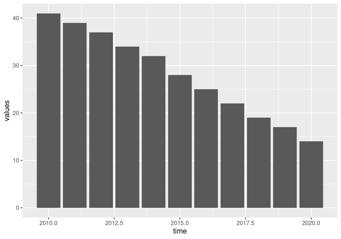
Figure 2.1: (ref:tin0028-italy-1)
Or, with a bit decoration:
tin00028 %>%
  filter(geo == 'IT') %>%
filter(indic_is == 'I_IUX') %>%
ggplot(aes(x = time, y = values)) +
geom_col(fill = "#336633") +
theme_bw() +
theme(text = element_text(size = 14)) +
labs(x = "Year", y = "% of population",
title = "Italians that never used Internet",
subtitle = "% of population of age 16-74")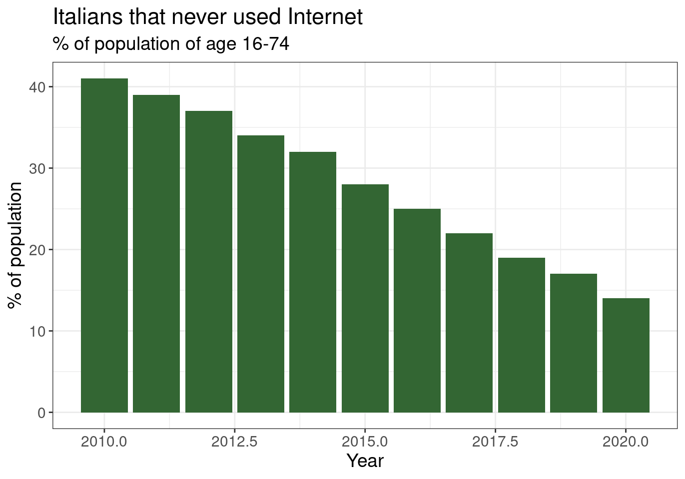
Figure 2.2: (ref:tin0028-italy-2)
2.3.2 Compare Italy with Austria
One can easily understand that change IT to AT can lead to a chart displaying the corresponding information about Austria:
tin00028 %>%
  filter(geo == 'AT') %>%
  filter(indic_is == 'I_IUX') %>%
  ggplot(aes(x = time, y = values)) +
  geom_col(fill = "#336633") +
  theme_bw() +
  theme(text = element_text(size = 14)) +
  labs(x = "Year", y = "% of population",
       title = "Austrians that never used Internet",
       subtitle = "% of population of age 16-74")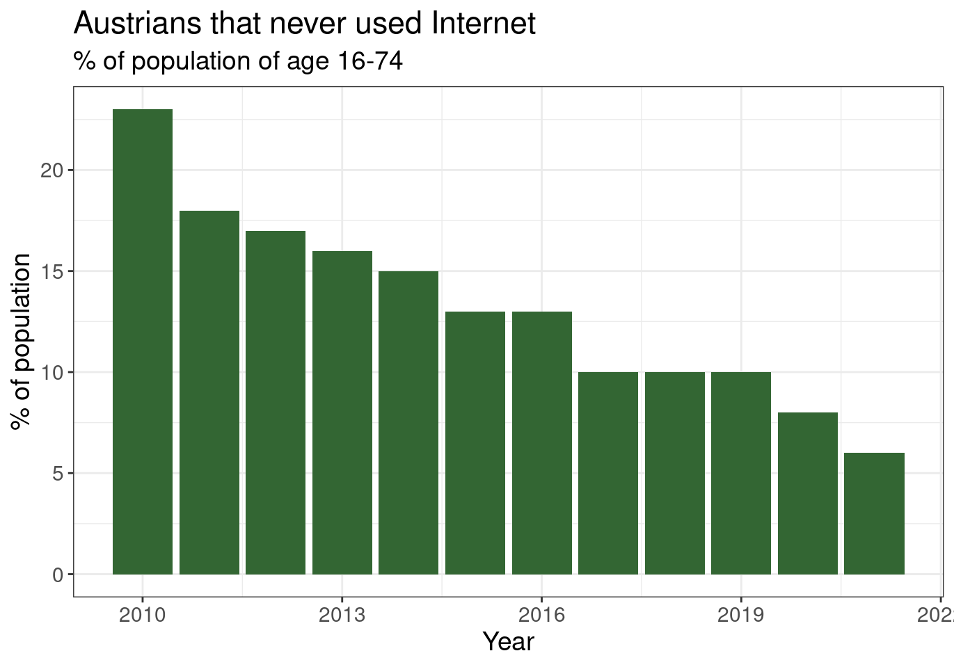
Figure 2.3: (ref:tin0028-italy-2)
What about if we try to compare Italy and Austria in one chart. The first step is to ensure that get the correct data. For example, one approach is:
## # A tibble: 23 × 6
##    ind_type  unit   indic_is geo    time values
##    <chr>     <chr>  <chr>    <chr> <dbl>  <dbl>
##  1 IND_TOTAL PC_IND I_IUX    AT     2010     23
##  2 IND_TOTAL PC_IND I_IUX    IT     2010     41
##  3 IND_TOTAL PC_IND I_IUX    AT     2011     18
##  4 IND_TOTAL PC_IND I_IUX    IT     2011     39
##  5 IND_TOTAL PC_IND I_IUX    AT     2012     17
##  6 IND_TOTAL PC_IND I_IUX    IT     2012     37
##  7 IND_TOTAL PC_IND I_IUX    AT     2013     16
##  8 IND_TOTAL PC_IND I_IUX    IT     2013     34
##  9 IND_TOTAL PC_IND I_IUX    AT     2014     15
## 10 IND_TOTAL PC_IND I_IUX    IT     2014     32
## # … with 13 more rows
Another more elegant approach is:
## # A tibble: 23 × 6
##    ind_type  unit   indic_is geo    time values
##    <chr>     <chr>  <chr>    <chr> <dbl>  <dbl>
##  1 IND_TOTAL PC_IND I_IUX    AT     2010     23
##  2 IND_TOTAL PC_IND I_IUX    IT     2010     41
##  3 IND_TOTAL PC_IND I_IUX    AT     2011     18
##  4 IND_TOTAL PC_IND I_IUX    IT     2011     39
##  5 IND_TOTAL PC_IND I_IUX    AT     2012     17
##  6 IND_TOTAL PC_IND I_IUX    IT     2012     37
##  7 IND_TOTAL PC_IND I_IUX    AT     2013     16
##  8 IND_TOTAL PC_IND I_IUX    IT     2013     34
##  9 IND_TOTAL PC_IND I_IUX    AT     2014     15
## 10 IND_TOTAL PC_IND I_IUX    IT     2014     32
## # … with 13 more rows
The former approach with the in is always preferable because of one single reason: It can be used in all cases whatever is the number of countries. For example this is an even better approach:
## # A tibble: 23 × 6
##    ind_type  unit   indic_is geo    time values
##    <chr>     <chr>  <chr>    <chr> <dbl>  <dbl>
##  1 IND_TOTAL PC_IND I_IUX    AT     2010     23
##  2 IND_TOTAL PC_IND I_IUX    IT     2010     41
##  3 IND_TOTAL PC_IND I_IUX    AT     2011     18
##  4 IND_TOTAL PC_IND I_IUX    IT     2011     39
##  5 IND_TOTAL PC_IND I_IUX    AT     2012     17
##  6 IND_TOTAL PC_IND I_IUX    IT     2012     37
##  7 IND_TOTAL PC_IND I_IUX    AT     2013     16
##  8 IND_TOTAL PC_IND I_IUX    IT     2013     34
##  9 IND_TOTAL PC_IND I_IUX    AT     2014     15
## 10 IND_TOTAL PC_IND I_IUX    IT     2014     32
## # … with 13 more rows
By changing and adapting the values of the cntr vector there is no need to care about the rest of the code.
Let’s see what we get:
tin00028 %>%
  filter(geo %in% cntr) %>%
  filter(indic_is == 'I_IUX') %>%
  ggplot(aes(x = time, y = values)) +
  geom_col() +
  theme_bw() +
  theme(text = element_text(size = 14)) +
  labs(x = "Year", y = "% of population",
       title = "Austrians and Italians that never used Internet",
       subtitle = "% of population of age 16-74")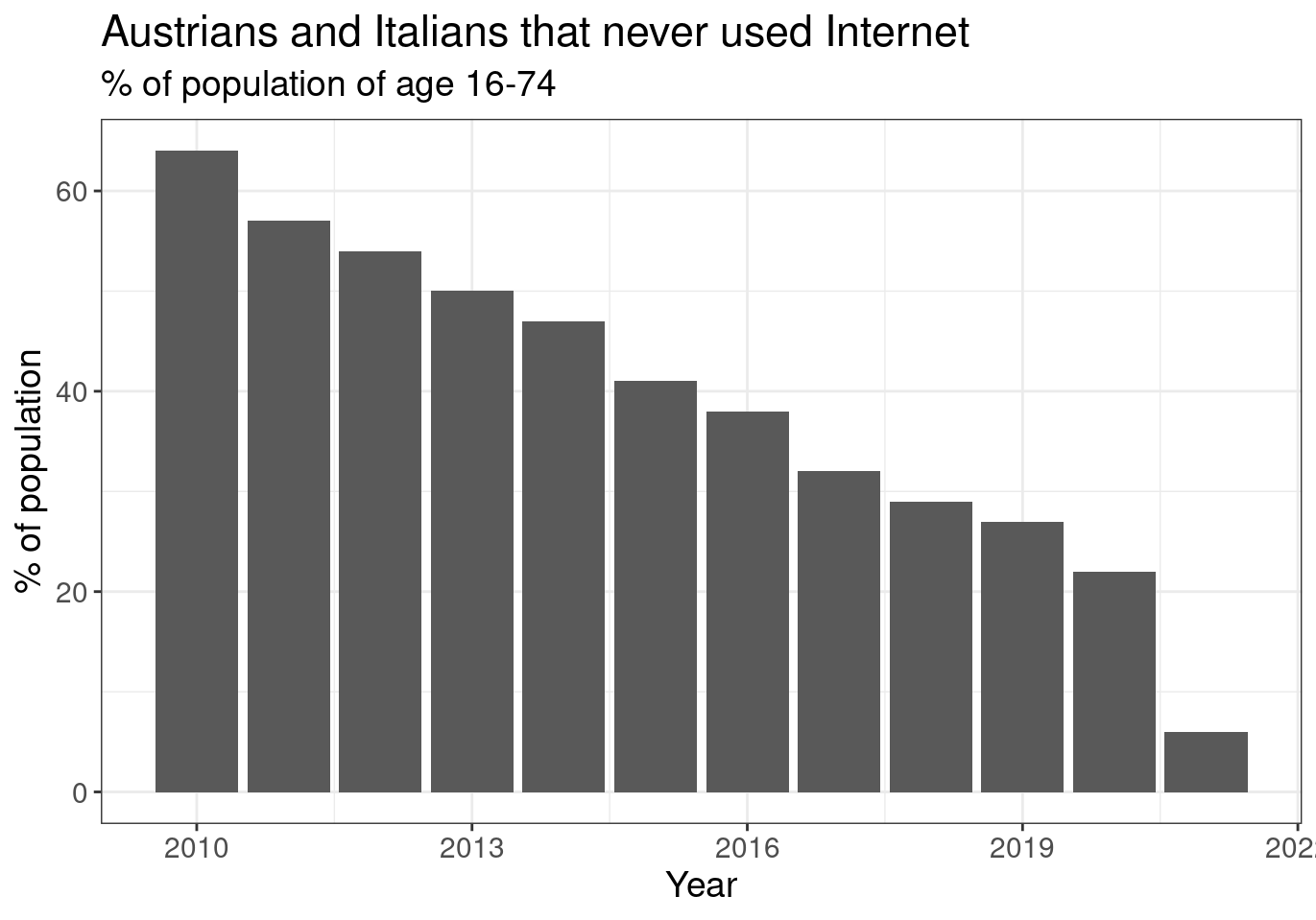
Figure 2.4: (ref:tin0028-italy-austria-1)
We still see one column. Why? Because we haven’t grouped the data by geo. We need to do so. This is done by one single option in aesthetics of the plot:
Since we present the data with columns/bars filled with a certain color, we need to instruct ggplot to do so:
tin00028 %>%
  filter(geo %in% cntr) %>%
  filter(indic_is == 'I_IUX') %>%
  ggplot(aes(x = time, y = values, fill = geo)) +
  geom_col() +
  theme_bw() +
  theme(text = element_text(size = 14)) +
  labs(x = "Year", y = "% of population",
       title = "Austrians and Italians that never used Internet",
       subtitle = "% of population of age 16-74")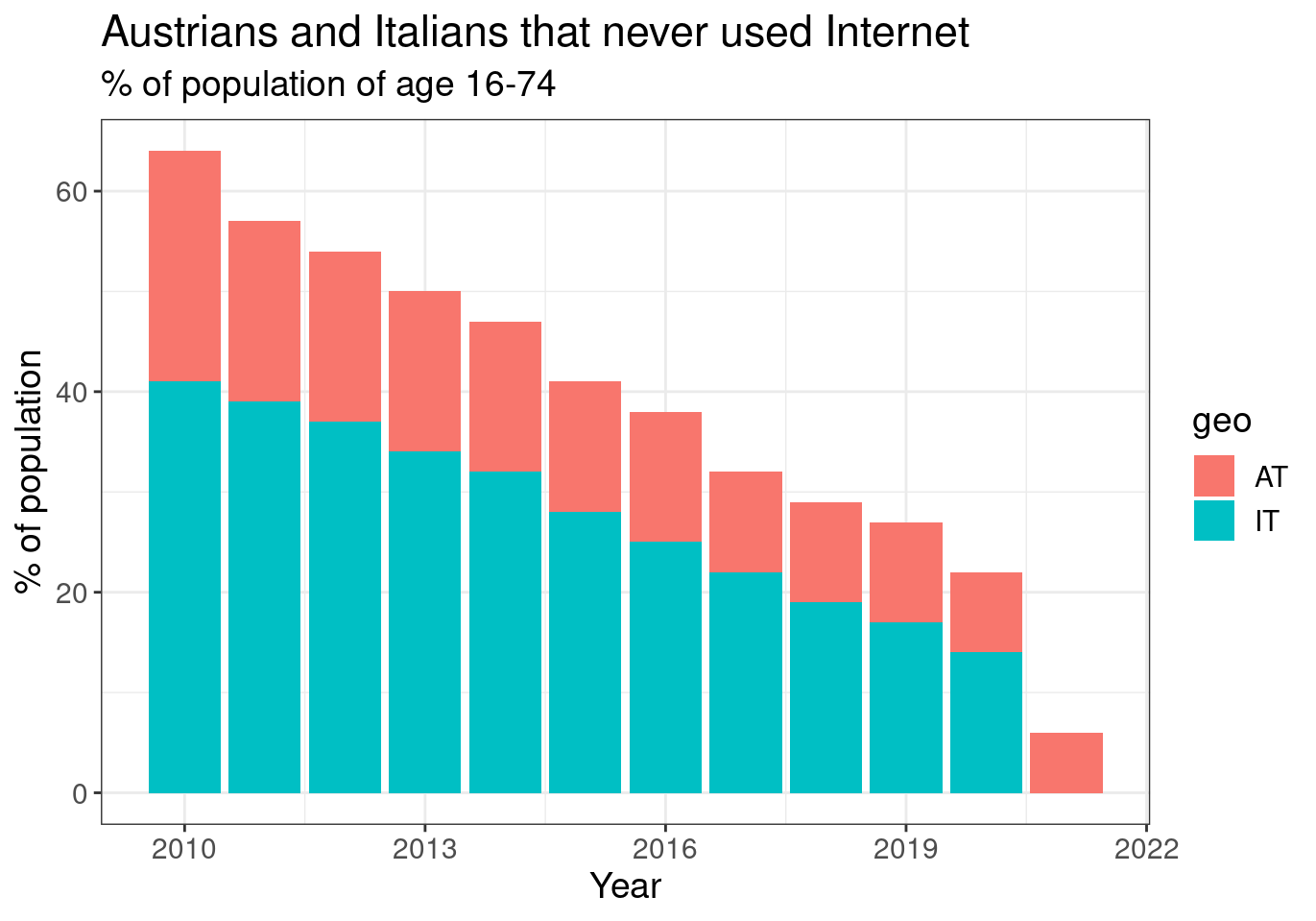
Figure 2.5: (ref:tin0028-italy-austria-2)
It looks better now, but still not satisfactory. Stacked columns is not exactly we would like to have in this chart. Having the bars side by would be much better. So the required option is:
So the chart can be made like this:
tin00028 %>%
  filter(geo %in% cntr) %>%
  filter(indic_is == 'I_IUX') %>%
  ggplot(aes(x = time, y = values, fill = geo)) +
  geom_col(position = "dodge") +
  theme_bw() +
  theme(text = element_text(size = 14)) +
  labs(x = "Year", y = "% of population",
       title = "Austrians and Italians that never used Internet",
       subtitle = "% of population of age 16-74")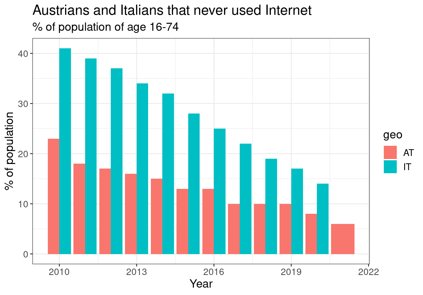
Figure 2.6: (ref:tin0028-italy-austria-3)
We can now clearly see that Austria has always had fewer percentage of its population that did not used internet, but also this percentage is declining over the years in both countries.
One more comment at this point. We used columns for geometrical representation of the data, so distinguish them by fill. In other such as points, lines, etc, with to use colour:
For example:
tin00028 %>%
  filter(geo %in% cntr) %>%
  filter(indic_is == 'I_IUX') %>%
  ggplot(aes(x = time, y = values, colour = geo)) +
  geom_line() +
  geom_point(size = 2) +
  theme_bw() +
  theme(text = element_text(size = 14)) +
  labs(x = "Year", y = "% of population",
       title = "Austrians and Italians that never used Internet",
       subtitle = "% of population of age 16-74")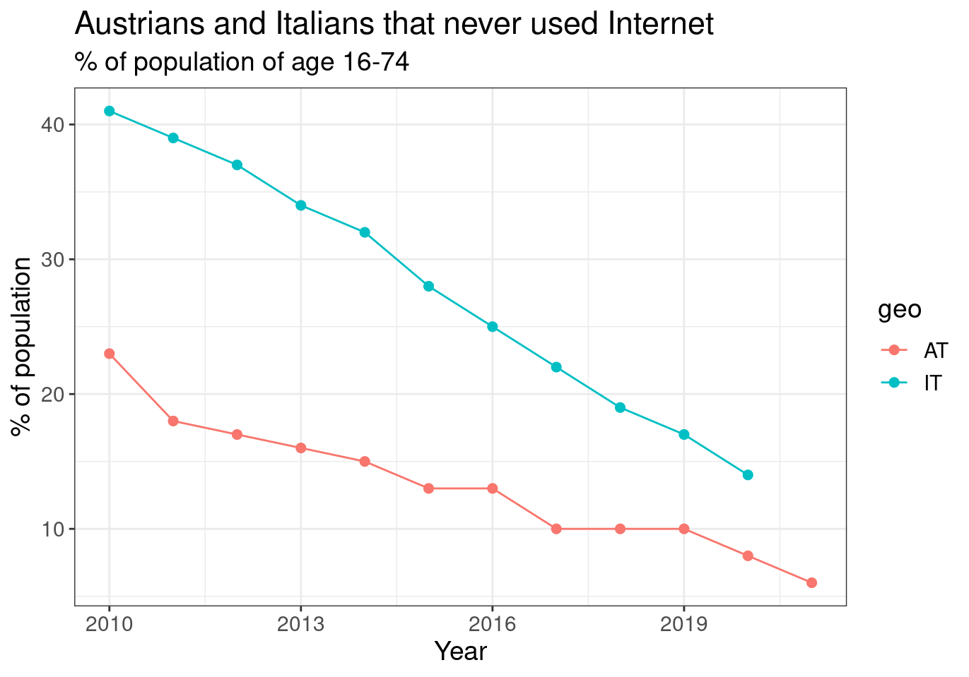
Figure 2.7: (ref:tin0028-italy-austria-4)
No need to use both lines and points all of the time. Certainly can be only one of them according to user preferences. Also in the above example, it is easy to understand that size in geom_point controls the size of points. Default value is 1, so b assigning the value of 2 we get double the size of the points.
2.3.3 Changing the default colors.
In cases like the previous one, the most wanted feature is adapting the colors of the plot. The interested reader can find more in-depth coverage of this topic elsewhere, in more relevant books. However we can grab the opportunity to give most commonly applied solutions.
One solution is to use one of brewer color schemes. There are 8 color schemes, here we see an example (with number 6):
tin00028 %>%
  filter(geo %in% cntr) %>%
  filter(indic_is == 'I_IUX') %>%
  ggplot(aes(x = time, y = values, fill = geo)) +
  geom_col(position = "dodge") +
  theme_bw() +
  theme(text = element_text(size = 14)) +
  scale_fill_brewer(palette = 6, type = "qual") +
  labs(x = "Year", y = "% of population",
       title = "Austrians and Italians that never used Internet",
       subtitle = "% of population of age 16-74")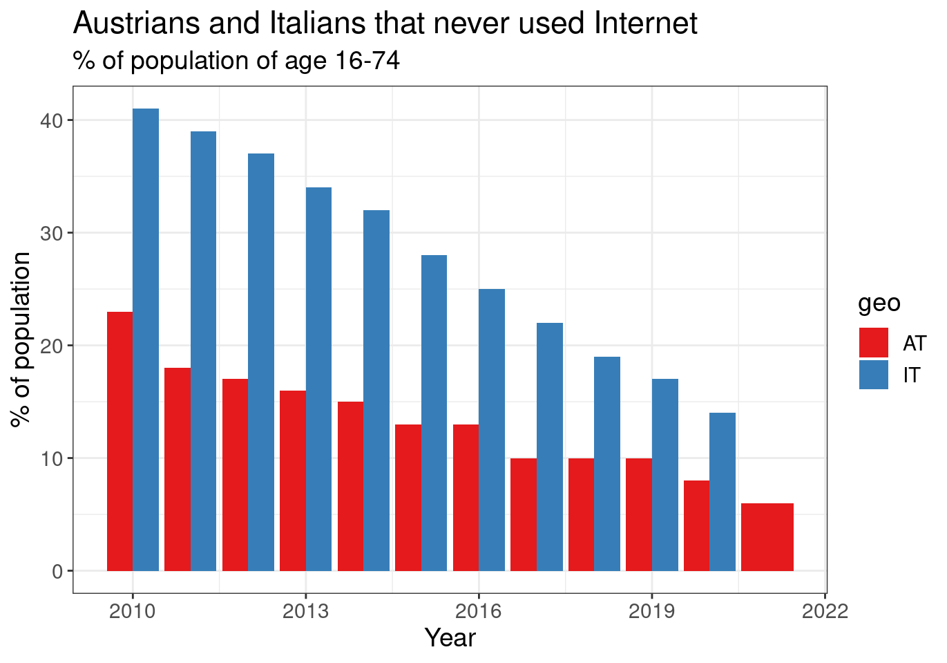
Figure 2.8: (ref:tin0028-italy-austria-4)
Another option is to change the theme. Library ggthemes offers many alternative themes. It can called:
And various color schemes can be used. For example the colors used by the Wall Street Journal:
tin00028 %>%
  filter(geo %in% cntr) %>%
  filter(indic_is == 'I_IUX') %>%
  ggplot(aes(x = time, y = values, fill = geo)) +
  geom_col(position = "dodge") +
  theme_bw() +
  theme(text = element_text(size = 14)) +
  scale_fill_wsj() +
  labs(x = "Year", y = "% of population",
       title = "Austrians and Italians that never used Internet",
       subtitle = "% of population of age 16-74")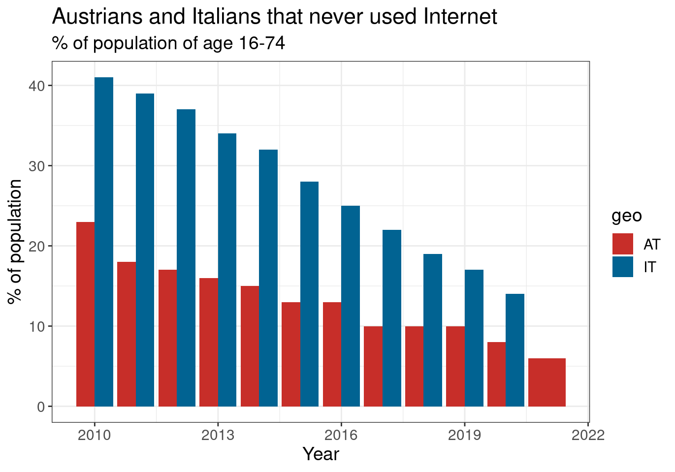
Figure 2.9: (ref:tin0028-italy-austria-4)
And another option could be the manual selection of colors. This is not my advice, but in case one needs to do so here is way:
tin00028 %>%
  filter(geo %in% cntr) %>%
  filter(indic_is == 'I_IUX') %>%
  ggplot(aes(x = time, y = values, fill = geo)) +
  geom_col(position = "dodge") +
  theme_bw() +
  theme(text = element_text(size = 14)) +
  scale_fill_manual(values = c("#FF0000", "#2E8B57")) +
  labs(x = "Year", y = "% of population",
       title = "Austrians and Italians that never used Internet",
       subtitle = "% of population of age 16-74")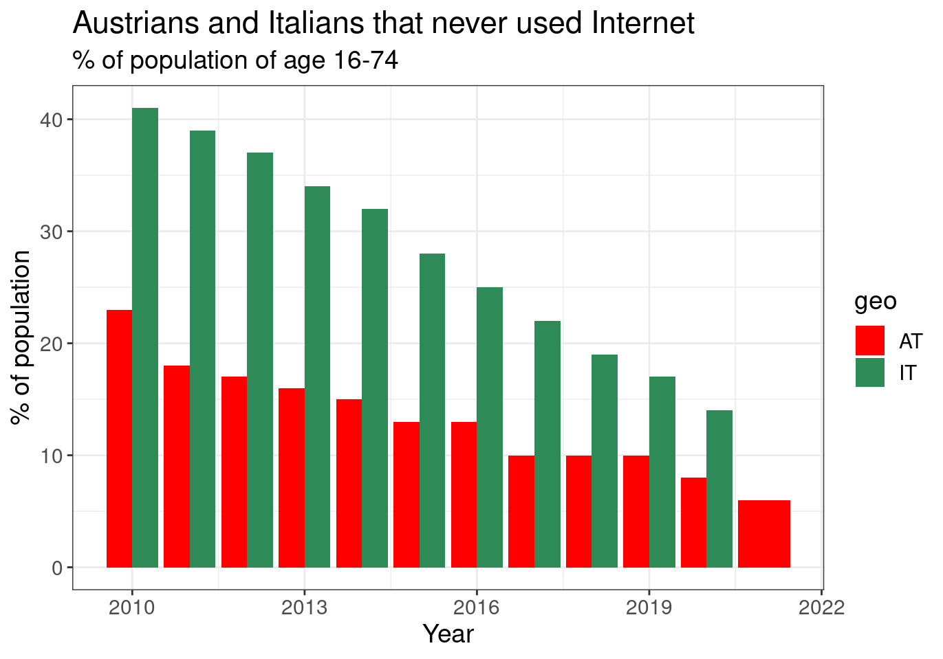
Figure 2.10: (ref:tin0028-italy-austria-4)