6 Labour force statistics

Here are some examples from the labour force statistics, about employment and unemployment.

Libraries we will need:

library(tidyverse)
library(eurostat)
library(lubridate)
library(ggthemes)
library(ggiraphExtra)
library(leaflet)
library(sf)

6.1 Annual unemployment of one country.

une <- get_eurostat("une_rt_a", 
             stringsAsFactors = FALSE,
             time_format = "num")

Here is the dataset:

une

## # A tibble: 22,881 × 6
##    age    unit   sex   geo    time values
##    <chr>  <chr>  <chr> <chr> <dbl>  <dbl>
##  1 Y15-24 PC_ACT F     AT     2020    9.5
##  2 Y15-24 PC_ACT F     BE     2020   15.1
##  3 Y15-24 PC_ACT F     BG     2020   13.7
##  4 Y15-24 PC_ACT F     CH     2020    8  
##  5 Y15-24 PC_ACT F     CY     2020   12.3
##  6 Y15-24 PC_ACT F     CZ     2020    9.2
##  7 Y15-24 PC_ACT F     DE     2020    6.7
##  8 Y15-24 PC_ACT F     DK     2020   10.6
##  9 Y15-24 PC_ACT F     EA19   2020   17.9
## 10 Y15-24 PC_ACT F     EE     2020   18.4
## # … with 22,871 more rows

Now, let’s start filtering the data.

1. Filter only for one country, here for Greece:

   une %>% 
     filter(geo == 'EL') 

   ## # A tibble: 648 × 6
   ##    age    unit    sex   geo    time values
   ##    <chr>  <chr>   <chr> <chr> <dbl>  <dbl>
   ##  1 Y15-24 PC_ACT  F     EL     2020   39.3
   ##  2 Y15-24 PC_ACT  M     EL     2020   31.4
   ##  3 Y15-24 PC_ACT  T     EL     2020   35  
   ##  4 Y15-24 PC_POP  F     EL     2020    7.6
   ##  5 Y15-24 PC_POP  M     EL     2020    7.3
   ##  6 Y15-24 PC_POP  T     EL     2020    7.4
   ##  7 Y15-24 THS_PER F     EL     2020   39  
   ##  8 Y15-24 THS_PER M     EL     2020   38  
   ##  9 Y15-24 THS_PER T     EL     2020   77  
   ## 10 Y15-74 PC_ACT  F     EL     2020   19.8
   ## # … with 638 more rows

2. For all age groups:

   une %>% 
     filter(geo == 'EL') %>% 
     filter(age == 'Y20-64')

   ## # A tibble: 108 × 6
   ##    age    unit    sex   geo    time values
   ##    <chr>  <chr>   <chr> <chr> <dbl>  <dbl>
   ##  1 Y20-64 PC_ACT  F     EL     2020   19.8
   ##  2 Y20-64 PC_ACT  M     EL     2020   13.6
   ##  3 Y20-64 PC_ACT  T     EL     2020   16.4
   ##  4 Y20-64 PC_POP  F     EL     2020   12.8
   ##  5 Y20-64 PC_POP  M     EL     2020   11.1
   ##  6 Y20-64 PC_POP  T     EL     2020   12  
   ##  7 Y20-64 THS_PER F     EL     2020  398  
   ##  8 Y20-64 THS_PER M     EL     2020  340  
   ##  9 Y20-64 THS_PER T     EL     2020  737  
   ## 10 Y20-64 PC_ACT  F     EL     2019   21.6
   ## # … with 98 more rows

3. For all both males and females:

   une %>% 
     filter(geo == 'EL') %>% 
     filter(age == 'Y20-64') %>% 
     filter(sex == 'T')

   ## # A tibble: 36 × 6
   ##    age    unit    sex   geo    time values
   ##    <chr>  <chr>   <chr> <chr> <dbl>  <dbl>
   ##  1 Y20-64 PC_ACT  T     EL     2020   16.4
   ##  2 Y20-64 PC_POP  T     EL     2020   12  
   ##  3 Y20-64 THS_PER T     EL     2020  737  
   ##  4 Y20-64 PC_ACT  T     EL     2019   17.3
   ##  5 Y20-64 PC_POP  T     EL     2019   12.8
   ##  6 Y20-64 THS_PER T     EL     2019  799  
   ##  7 Y20-64 PC_ACT  T     EL     2018   19.3
   ##  8 Y20-64 PC_POP  T     EL     2018   14.2
   ##  9 Y20-64 THS_PER T     EL     2018  892  
   ## 10 Y20-64 PC_ACT  T     EL     2017   21.4
   ## # … with 26 more rows

4. And take into account percentage of active population:

   une %>% 
     filter(geo == 'EL') %>% 
     filter(age == 'Y20-64') %>% 
     filter(sex == 'T')  %>% 
     filter(unit == 'PC_ACT')

   ## # A tibble: 12 × 6
   ##    age    unit   sex   geo    time values
   ##    <chr>  <chr>  <chr> <chr> <dbl>  <dbl>
   ##  1 Y20-64 PC_ACT T     EL     2020   16.4
   ##  2 Y20-64 PC_ACT T     EL     2019   17.3
   ##  3 Y20-64 PC_ACT T     EL     2018   19.3
   ##  4 Y20-64 PC_ACT T     EL     2017   21.4
   ##  5 Y20-64 PC_ACT T     EL     2016   23.5
   ##  6 Y20-64 PC_ACT T     EL     2015   24.9
   ##  7 Y20-64 PC_ACT T     EL     2014   26.4
   ##  8 Y20-64 PC_ACT T     EL     2013   27.3
   ##  9 Y20-64 PC_ACT T     EL     2012   24.3
   ## 10 Y20-64 PC_ACT T     EL     2011   17.8
   ## 11 Y20-64 PC_ACT T     EL     2010   12.7
   ## 12 Y20-64 PC_ACT T     EL     2009    9.5

Finally, store the results for further usage:

cntr_une <- une %>% 
  filter(geo == 'EL') %>% 
  filter(age == 'Y20-64') %>% 
  filter(sex == 'T')  %>% 
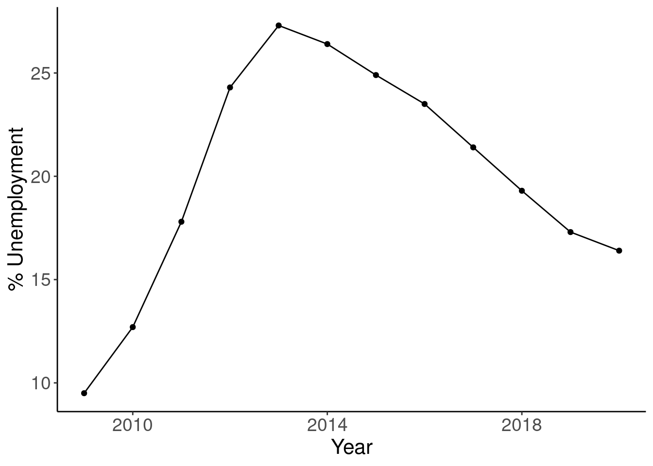
  filter(unit == 'PC_ACT')

### Simple plots

 ggplot(cntr_une, aes(x = time, y = values)) +
   geom_col()

 ggplot(cntr_une, aes(x = time, y = values)) +
   geom_line() +
   geom_point()

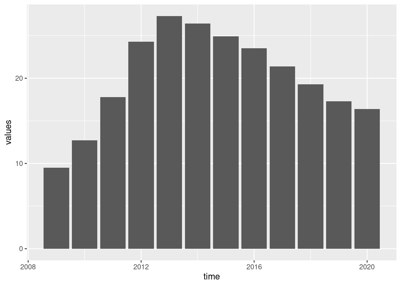
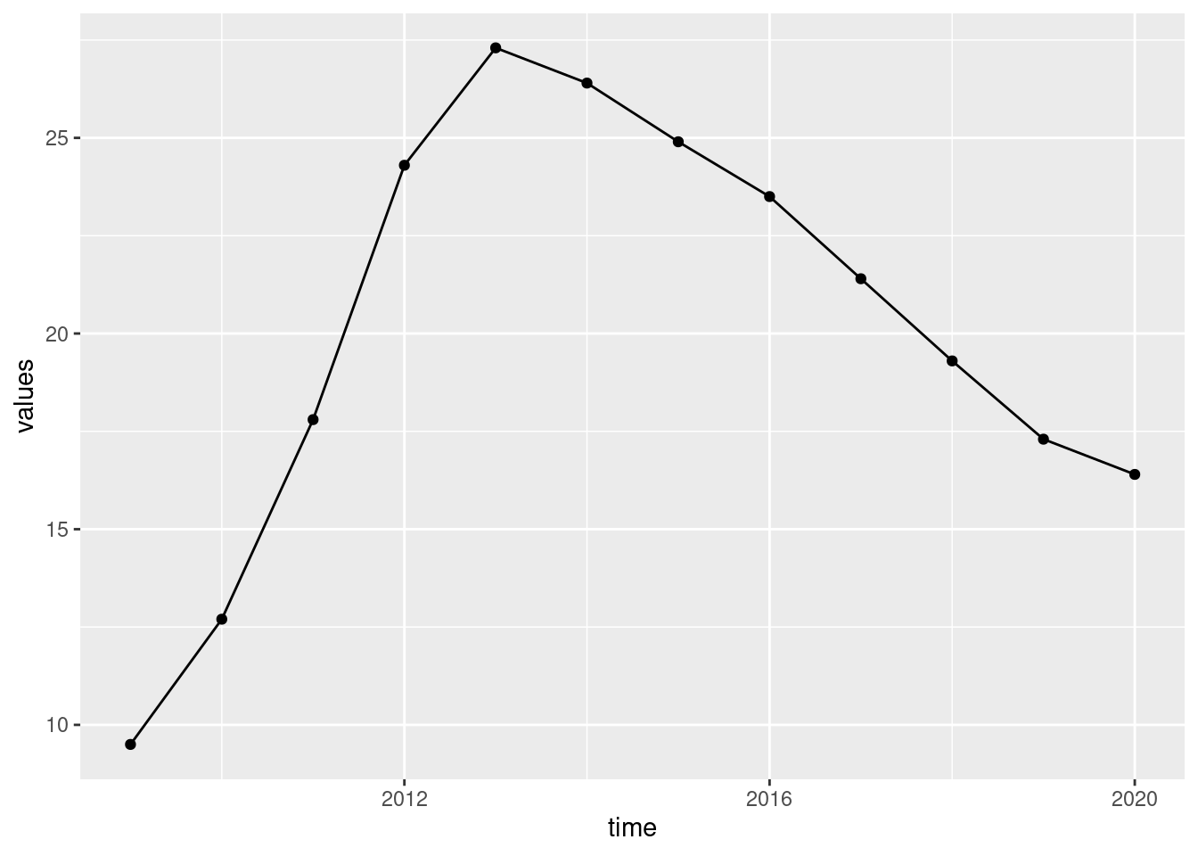
 ggplot(cntr_une, aes(x = time, y = values)) +
   geom_line() +
   geom_point() +
   labs(x = "Year", y = "% Unemployment") +
   scale_x_continuous(breaks = seq(1998, 2020, by = 4)) +
   theme_classic() +
   theme(
     text = element_text(size = 16),
     axis.text = element_text(size = 14)
   )

6.1.1 Male nad female unemployment

Now lets separate male and female unemployment.

6.2 Quarterly unemployment of one country.

cntr_une <- une %>% 
  filter(geo == 'EL') %>% 
  filter(age == 'Y20-64') %>% 
  filter(sex %in% c('F', 'M'))  %>% 
  filter(unit == 'PC_ACT')

Attention now, we have two values for each time and geo:

 cntr_une

## # A tibble: 24 × 6
##    age    unit   sex   geo    time values
##    <chr>  <chr>  <chr> <chr> <dbl>  <dbl>
##  1 Y20-64 PC_ACT F     EL     2020   19.8
##  2 Y20-64 PC_ACT M     EL     2020   13.6
##  3 Y20-64 PC_ACT F     EL     2019   21.6
##  4 Y20-64 PC_ACT M     EL     2019   13.9
##  5 Y20-64 PC_ACT F     EL     2018   24.2
##  6 Y20-64 PC_ACT M     EL     2018   15.3
##  7 Y20-64 PC_ACT F     EL     2017   26  
##  8 Y20-64 PC_ACT M     EL     2017   17.8
##  9 Y20-64 PC_ACT F     EL     2016   28.1
## 10 Y20-64 PC_ACT M     EL     2016   19.7
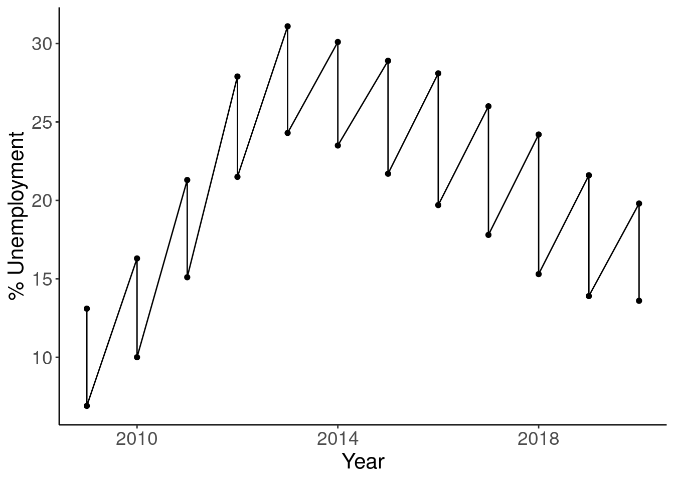
## # … with 14 more rows

If we plot the data as previously, then we got a wrong plot:

 ggplot(cntr_une, aes(x = time, y = values)) +
   geom_line() +
   geom_point() +
   labs(x = "Year", y = "% Unemployment") +
   scale_x_continuous(breaks = seq(1998, 2020, by = 4)) +
   theme_classic() +
   theme(
     text = element_text(size = 16),
     axis.text = element_text(size = 14)
   )

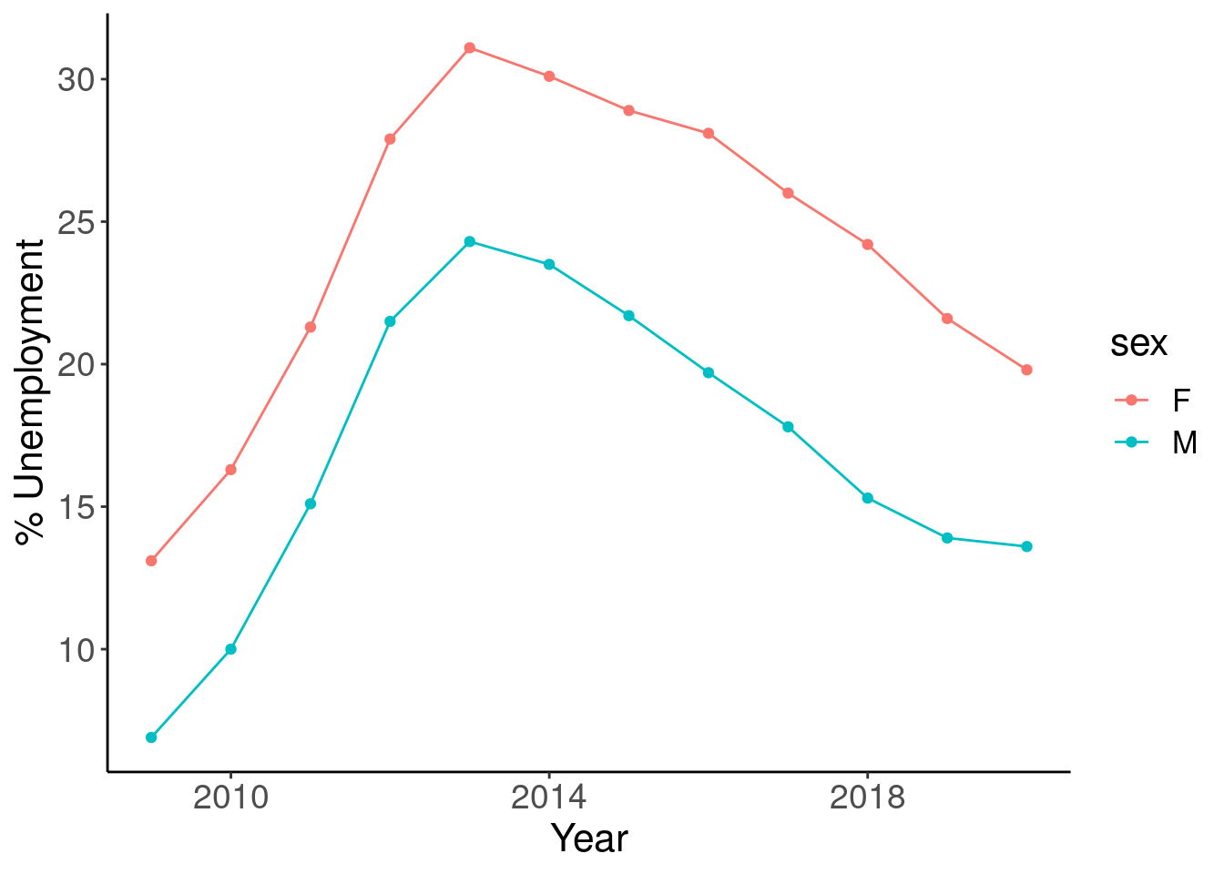
We have to define the aesthetics:

 ggplot(cntr_une, aes(x = time, y = values, colour = sex)) +
   geom_line() +
   geom_point() +
   labs(x = "Year", y = "% Unemployment") +
   scale_x_continuous(breaks = seq(1998, 2020, by = 4)) +
   theme_classic() +
   theme(
     text = element_text(size = 16),
     axis.text = element_text(size = 14)
   )

Now let’s take into account the total number, in thousands of persons:

cntr_une <- une %>% 
  filter(geo == 'EL') %>% 
  filter(age == 'Y20-64') %>% 
  filter(sex %in% c('F', 'M'))  %>% 
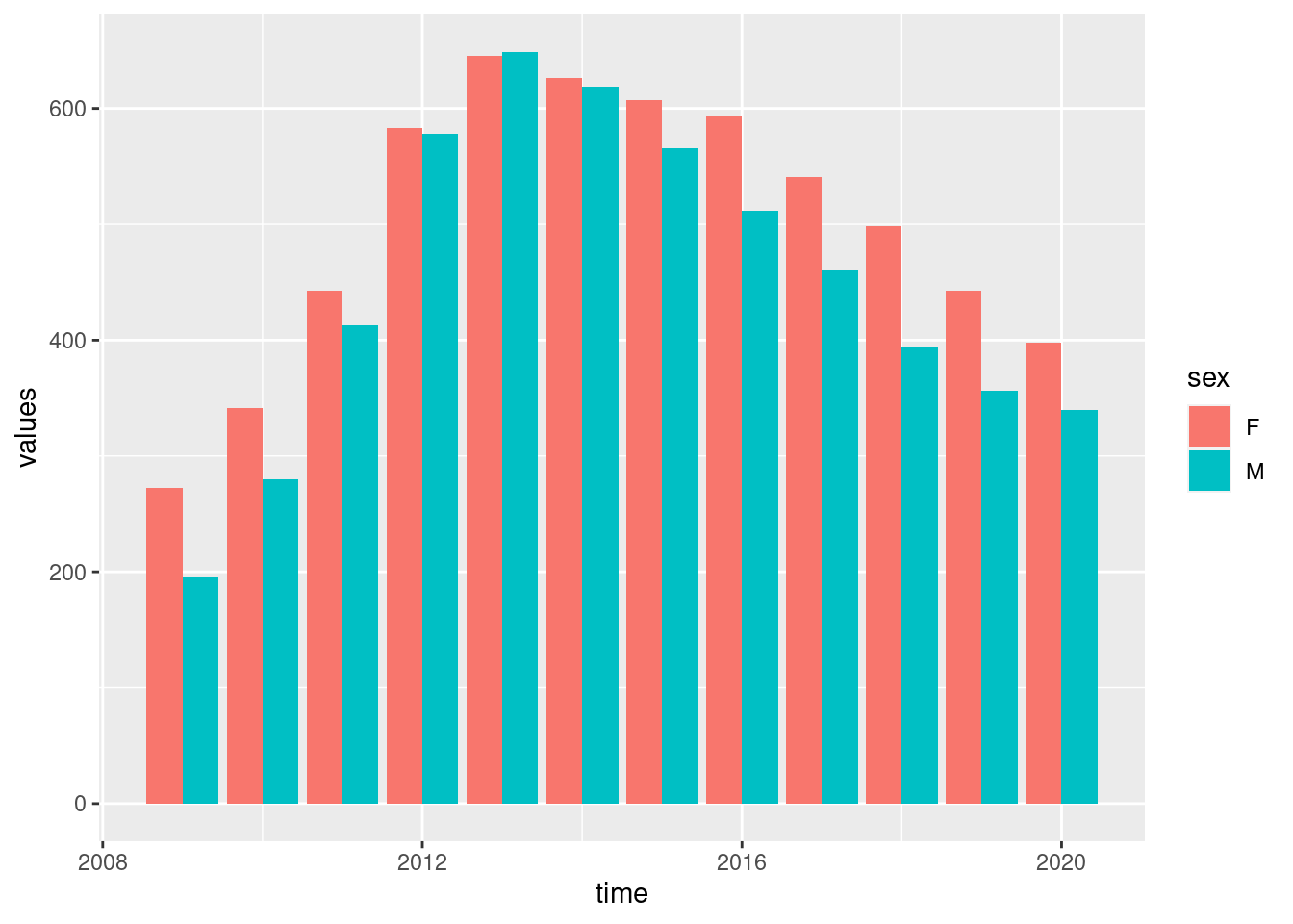
  filter(unit == 'THS_PER')

Plot the data:

ggplot(cntr_une, aes(x = time, y = values)) +
  geom_col()

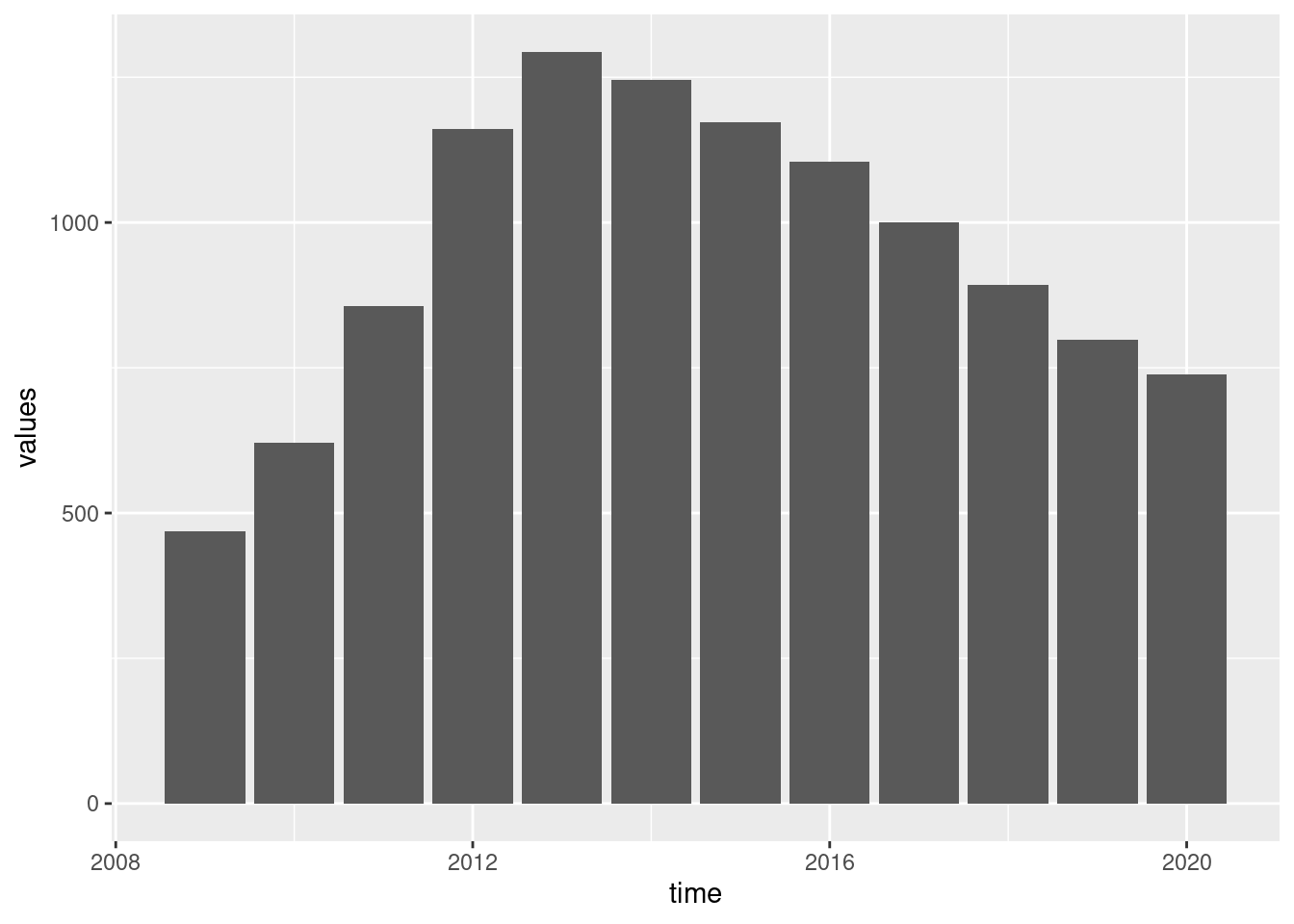
Plot the data in a more correct way:

ggplot(cntr_une, aes(x = time, y = values, fill = sex)) +
  geom_col()

or like this:

ggplot(cntr_une, aes(x = time, y = values, fill = sex)) +
  geom_col(position = "dodge")

6.2.1 Manipulating the dataset

Now a more difficult task. We have to calculate and plot the percentage of uneployed males and females. First of all we need to transform the data into two columns:

cntr_une %>% 
  pivot_wider(id_cols = c(geo, time, sex),
              names_from = sex,
              values_from = values)

## # A tibble: 12 × 4
##    geo    time     F     M
##    <chr> <dbl> <dbl> <dbl>
##  1 EL     2020   398   340
##  2 EL     2019   443   356
##  3 EL     2018   498   394
##  4 EL     2017   541   460
##  5 EL     2016   593   512
##  6 EL     2015   607   566
##  7 EL     2014   626   619
##  8 EL     2013   645   649
##  9 EL     2012   583   578
## 10 EL     2011   443   413
## 11 EL     2010   341   280
## 12 EL     2009   272   196

and then:

cntr_une %>% 
  pivot_wider(id_cols = c(geo, time, sex),
              names_from = sex,
              values_from = values) %>% 
  mutate(Female = 100*F/(F+M),
       Male = 100*M/(F+M))

## # A tibble: 12 × 6
##    geo    time     F     M Female  Male
##    <chr> <dbl> <dbl> <dbl>  <dbl> <dbl>
##  1 EL     2020   398   340   53.9  46.1
##  2 EL     2019   443   356   55.4  44.6
##  3 EL     2018   498   394   55.8  44.2
##  4 EL     2017   541   460   54.0  46.0
##  5 EL     2016   593   512   53.7  46.3
##  6 EL     2015   607   566   51.7  48.3
##  7 EL     2014   626   619   50.3  49.7
##  8 EL     2013   645   649   49.8  50.2
##  9 EL     2012   583   578   50.2  49.8
## 10 EL     2011   443   413   51.8  48.2
## 11 EL     2010   341   280   54.9  45.1
## 12 EL     2009   272   196   58.1  41.9

Afterthat, we have to put the data back into the previous format:

cntr_une_fm_perc <- cntr_une %>% 
  pivot_wider(id_cols = c(geo, time, sex),
              names_from = sex,
              values_from = values) %>% 
  mutate(Females = 100*F/(F+M),
         Males = 100*M/(F+M)) %>% 
  select(-c(F, M)) %>% 
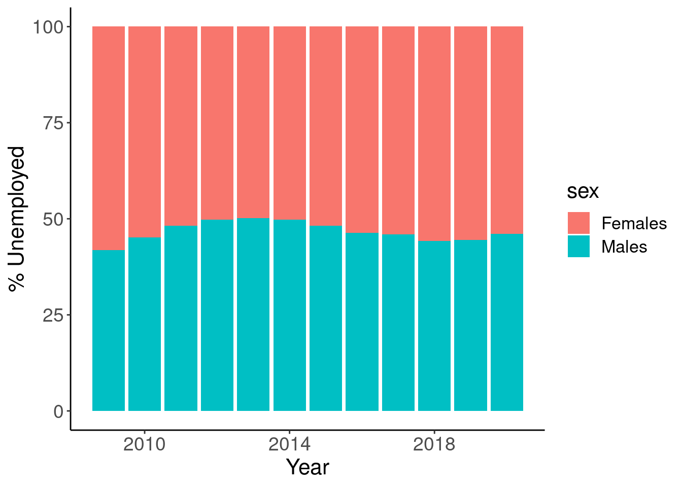
  pivot_longer(cols = c(Females, Males), names_to = "sex", values_to = "values")

Now we plot the data:

ggplot(cntr_une_fm_perc, aes(x = time, y = values, fill = sex)) +
  geom_col(position = "stack") +
  labs(x = "Year", y = "% Unemployed") +
  scale_x_continuous(breaks = seq(1998, 2020, by = 4)) +
  theme_classic() +
  theme(text = element_text(size = 16),
        axis.text = element_text(size = 14)
        )

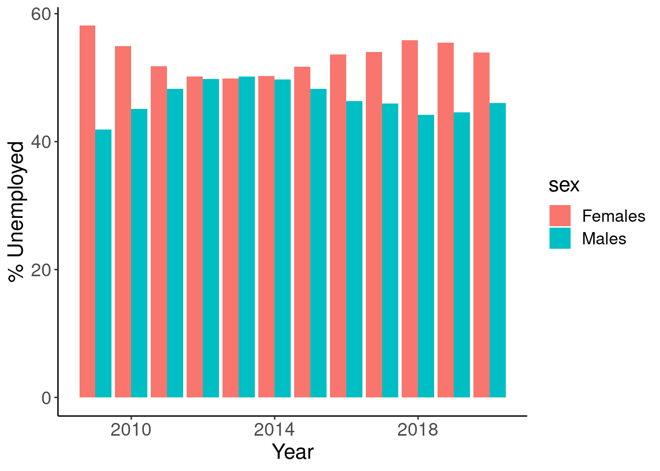
ggplot(cntr_une_fm_perc, aes(x = time, y = values, fill = sex)) +
  geom_col(position = "dodge") +
  labs(x = "Year", y = "% Unemployed") +
  scale_x_continuous(breaks = seq(1998, 2020, by = 4)) +
  theme_classic() +
  theme(text = element_text(size = 16),
        axis.text = element_text(size = 14)
        )

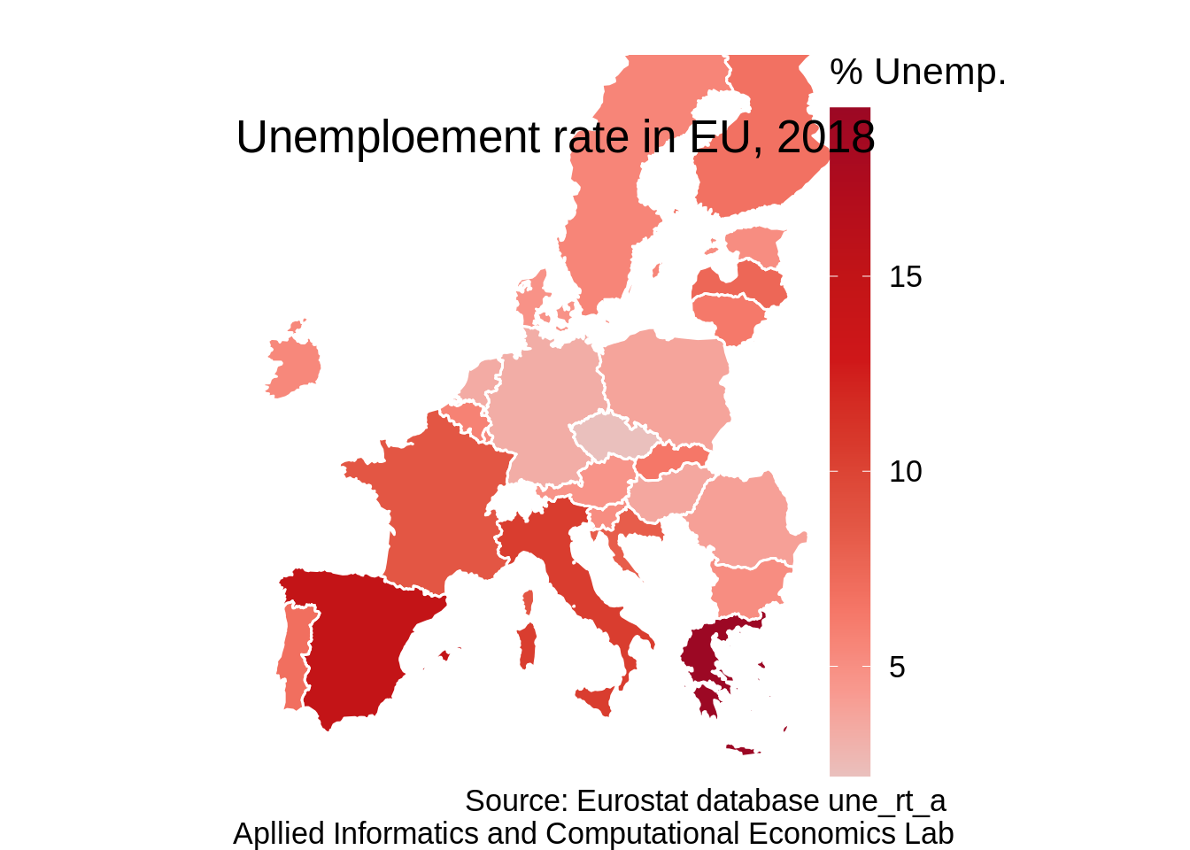
6.3 Annual data, map for multiple countries

Here is a tiny transformation of the eu_countries table

eu_countries <- eu_countries %>% 
  select(geo = code, cntr_name = name)

We will now join it with the unemployment data in order to keep only data for EU countries and also to have a new column with th country name (instead of the geo code):

une <- inner_join(eu_countries, une, by = "geo")

Now, we select the data for one year:

une_year <- une %>% 
  filter(time == 2018) %>% 
  filter(age == 'Y20-64') %>% 
  filter(sex == 'T')  %>% 
  filter(unit == 'PC_ACT')

One good plot coulf be like this:

ggplot(une_year, aes(x = geo, y = values)) +
  geom_col()

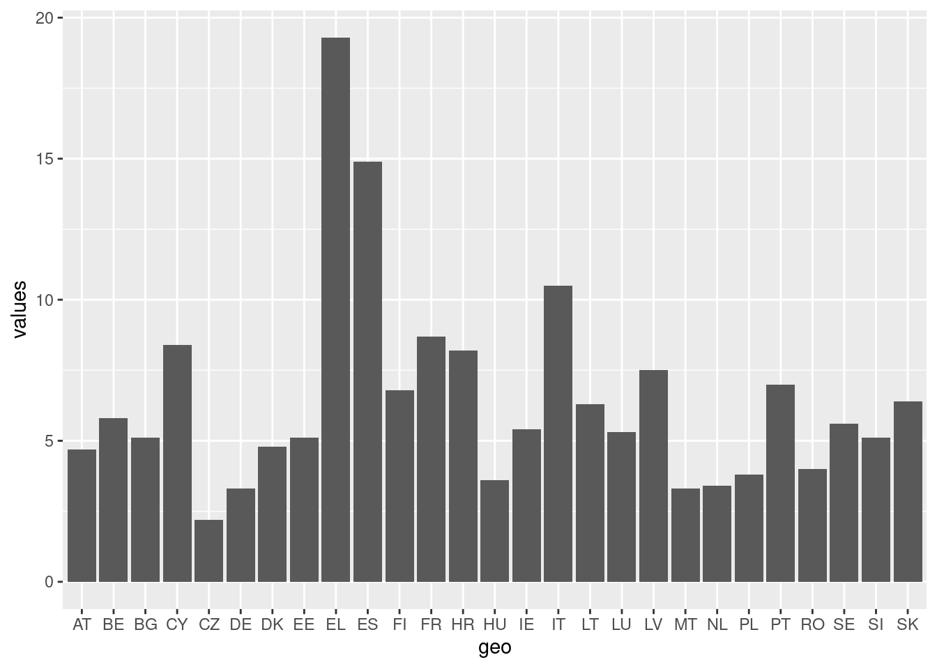
But it is even better like this:

ggplot(une_year, aes(x = reorder(geo, values), y = values)) +
  geom_col()

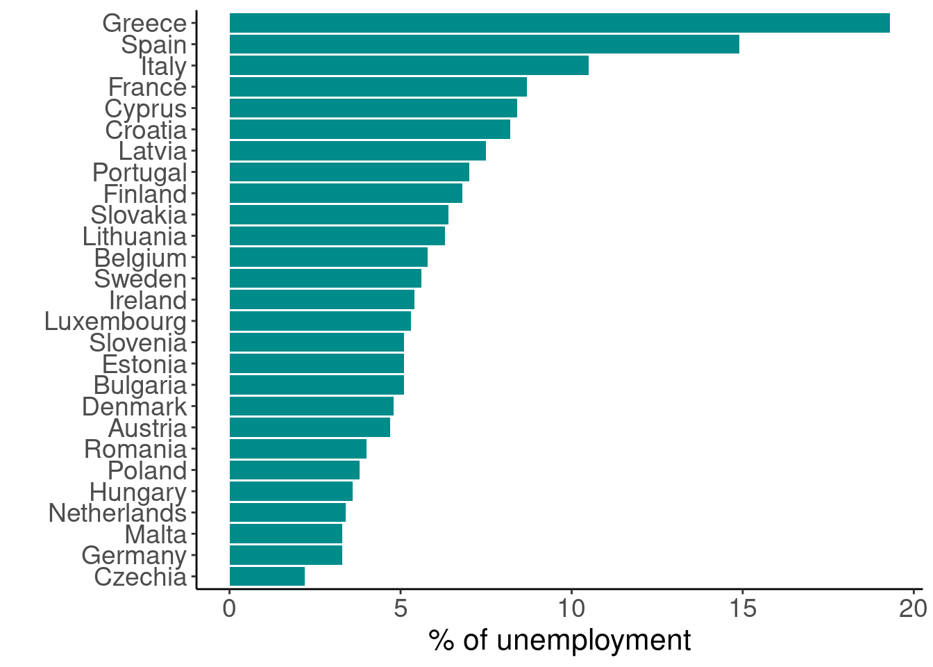
or even better:

ggplot(une_year, aes(x = reorder(cntr_name, values), y = values)) +
  geom_col(fill = "#008B8B") +
  coord_flip() +
  labs(x = "", y = "% of unemployment") +
  theme_classic() +
  theme(text = element_text(size = 16),
        axis.text = element_text(size = 14)
        )

6.3.1 Put the data on a map

Here is a plot we want to make:

SHP_0 <- get_eurostat_geospatial(resolution = 10, 
                                 nuts_level = 0, 
                                 year = 2016)

EU_SHP_0 <- inner_join(SHP_0, eu_countries, by = "geo")
DF <- inner_join(une_year, EU_SHP_0, by = "geo") %>% 
  st_as_sf()

ggplot(DF) +
  geom_sf(aes(fill = values), color = "white", size = 0) +
  geom_sf(data = EU_SHP_0, fill = NA, color = "white", size = 0.5) +
  scale_fill_continuous_tableau(palette = "Classic Red", breaks = seq(0, 80, by = 5), na.value="gray60") +
  xlim(-10.0, 38.0) + ylim(35.5, 66.0) +
  labs(title = "Unemploement rate in EU, 2018", 
       caption = "Source: Eurostat database une_rt_a 
                  Apllied Informatics and Computational Economics Lab",
       fill = "% Unemp.") +
  theme_void() +
  theme(text = element_text(size = 16, family = "Arial")) +
  theme(legend.key.height = unit(2, "cm")) +
  theme(legend.position = c(0.95, 0.5))+
  theme(plot.title = element_text(hjust = 0, vjust = -10)) +
  theme(plot.subtitle = element_text(hjust = 0, vjust = -14))