8 How to compare statistics

Libraries we will need:

library(tidyverse)
library(eurostat)
library(scales)
library(leaflet)
library(sf)
library(ggrepel)
library(ggpubr)
library(ggthemes)
library(hrbrthemes)

8.1 Internet access

Table tin00028 contains annual data and information about internet of European households. Let’s download:

iuse <- get_eurostat("tin00028", 
                     stringsAsFactors = FALSE,
                     time_format = "num")

## Table tin00028 cached at /tmp/RtmpwnUDOu/eurostat/tin00028_num_code_FF.rds

Also, we will rename the columns of the eu_countries table (embeded in eurostat package). Before:

head(eu_countries)

##   code     name                                            label
## 1   BE  Belgium                                          Belgium
## 2   BG Bulgaria                                         Bulgaria
## 3   CZ  Czechia                                          Czechia
## 4   DK  Denmark                                          Denmark
## 5   DE  Germany Germany (until 1990 former territory of the FRG)
## 6   EE  Estonia                                          Estonia

EU_countries <- select(eu_countries, geo = code, country = name)

After:

head(EU_countries)

##   geo  country
## 1  BE  Belgium
## 2  BG Bulgaria
## 3  CZ  Czechia
## 4  DK  Denmark
## 5  DE  Germany
## 6  EE  Estonia

Now, our target is to show the differences in internet access between 2015 and 2020 for all EU countries. We will take (initially) into consideration the index I_IU3, thus percentage of peope who had accessed internet during the previous three months.

Here is the dataset we have downloaded:

iuse

## # A tibble: 1,780 × 6
##    ind_type  unit   indic_is geo    time values
##    <chr>     <chr>  <chr>    <chr> <dbl>  <dbl>
##  1 IND_TOTAL PC_IND I_ILT12  AT     2010     75
##  2 IND_TOTAL PC_IND I_ILT12  BE     2010     79
##  3 IND_TOTAL PC_IND I_ILT12  BG     2010     46
##  4 IND_TOTAL PC_IND I_ILT12  CY     2010     53
##  5 IND_TOTAL PC_IND I_ILT12  CZ     2010     69
##  6 IND_TOTAL PC_IND I_ILT12  DE     2010     82
##  7 IND_TOTAL PC_IND I_ILT12  DK     2010     89
##  8 IND_TOTAL PC_IND I_ILT12  EA     2010     71
##  9 IND_TOTAL PC_IND I_ILT12  EE     2010     75
## 10 IND_TOTAL PC_IND I_ILT12  EL     2010     46
## # … with 1,770 more rows

If we join with eu_countries

iuse %>%
  inner_join(EU_countries, by = "geo")

## # A tibble: 1,332 × 7
##    ind_type  unit   indic_is geo    time values country 
##    <chr>     <chr>  <chr>    <chr> <dbl>  <dbl> <chr>   
##  1 IND_TOTAL PC_IND I_ILT12  AT     2010     75 Austria 
##  2 IND_TOTAL PC_IND I_ILT12  BE     2010     79 Belgium 
##  3 IND_TOTAL PC_IND I_ILT12  BG     2010     46 Bulgaria
##  4 IND_TOTAL PC_IND I_ILT12  CY     2010     53 Cyprus  
##  5 IND_TOTAL PC_IND I_ILT12  CZ     2010     69 Czechia 
##  6 IND_TOTAL PC_IND I_ILT12  DE     2010     82 Germany 
##  7 IND_TOTAL PC_IND I_ILT12  DK     2010     89 Denmark 
##  8 IND_TOTAL PC_IND I_ILT12  EE     2010     75 Estonia 
##  9 IND_TOTAL PC_IND I_ILT12  EL     2010     46 Greece  
## 10 IND_TOTAL PC_IND I_ILT12  ES     2010     66 Spain   
## # … with 1,322 more rows

we have now only EU countries (excluding Norway, Turkey, etc) and we have added and country name.

We start filtering the dataset now. First, include only two years:

iuse %>%
  inner_join(EU_countries, by = "geo") %>%
  filter(time %in% c(2015, 2020))

## # A tibble: 220 × 7
##    ind_type  unit   indic_is geo    time values country 
##    <chr>     <chr>  <chr>    <chr> <dbl>  <dbl> <chr>   
##  1 IND_TOTAL PC_IND I_ILT12  AT     2015     85 Austria 
##  2 IND_TOTAL PC_IND I_ILT12  BE     2015     86 Belgium 
##  3 IND_TOTAL PC_IND I_ILT12  BG     2015     60 Bulgaria
##  4 IND_TOTAL PC_IND I_ILT12  CY     2015     72 Cyprus  
##  5 IND_TOTAL PC_IND I_ILT12  CZ     2015     83 Czechia 
##  6 IND_TOTAL PC_IND I_ILT12  DE     2015     89 Germany 
##  7 IND_TOTAL PC_IND I_ILT12  DK     2015     97 Denmark 
##  8 IND_TOTAL PC_IND I_ILT12  EE     2015     89 Estonia 
##  9 IND_TOTAL PC_IND I_ILT12  EL     2015     68 Greece  
## 10 IND_TOTAL PC_IND I_ILT12  ES     2015     80 Spain   
## # … with 210 more rows

And then filtering for the I_IU3 index:

iuse %>%
  inner_join(EU_countries, by = "geo") %>%
  filter(time %in% c(2015, 2020)) %>%
  filter(indic_is == 'I_IU3')

## # A tibble: 55 × 7
##    ind_type  unit   indic_is geo    time values country 
##    <chr>     <chr>  <chr>    <chr> <dbl>  <dbl> <chr>   
##  1 IND_TOTAL PC_IND I_IU3    AT     2015     84 Austria 
##  2 IND_TOTAL PC_IND I_IU3    BE     2015     85 Belgium 
##  3 IND_TOTAL PC_IND I_IU3    BG     2015     57 Bulgaria
##  4 IND_TOTAL PC_IND I_IU3    CY     2015     72 Cyprus  
##  5 IND_TOTAL PC_IND I_IU3    CZ     2015     81 Czechia 
##  6 IND_TOTAL PC_IND I_IU3    DE     2015     88 Germany 
##  7 IND_TOTAL PC_IND I_IU3    DK     2015     96 Denmark 
##  8 IND_TOTAL PC_IND I_IU3    EE     2015     88 Estonia 
##  9 IND_TOTAL PC_IND I_IU3    EL     2015     67 Greece  
## 10 IND_TOTAL PC_IND I_IU3    ES     2015     79 Spain   
## # … with 45 more rows

We can skip filtering about the unit column because it contains only one value: PC_IND (percentage of individuals). Let’s store the intermediate results:

eu_iuse <- iuse %>%
  inner_join(EU_countries, by = "geo") %>%
  filter(time %in% c(2015, 2020)) %>%
  filter(indic_is == 'I_IU3')

And here is a first try to visualize the data:

ggplot(eu_iuse, aes(x = country, y = values, fill = as.factor(time))) +
  geom_col(position = "dodge") +
  coord_flip()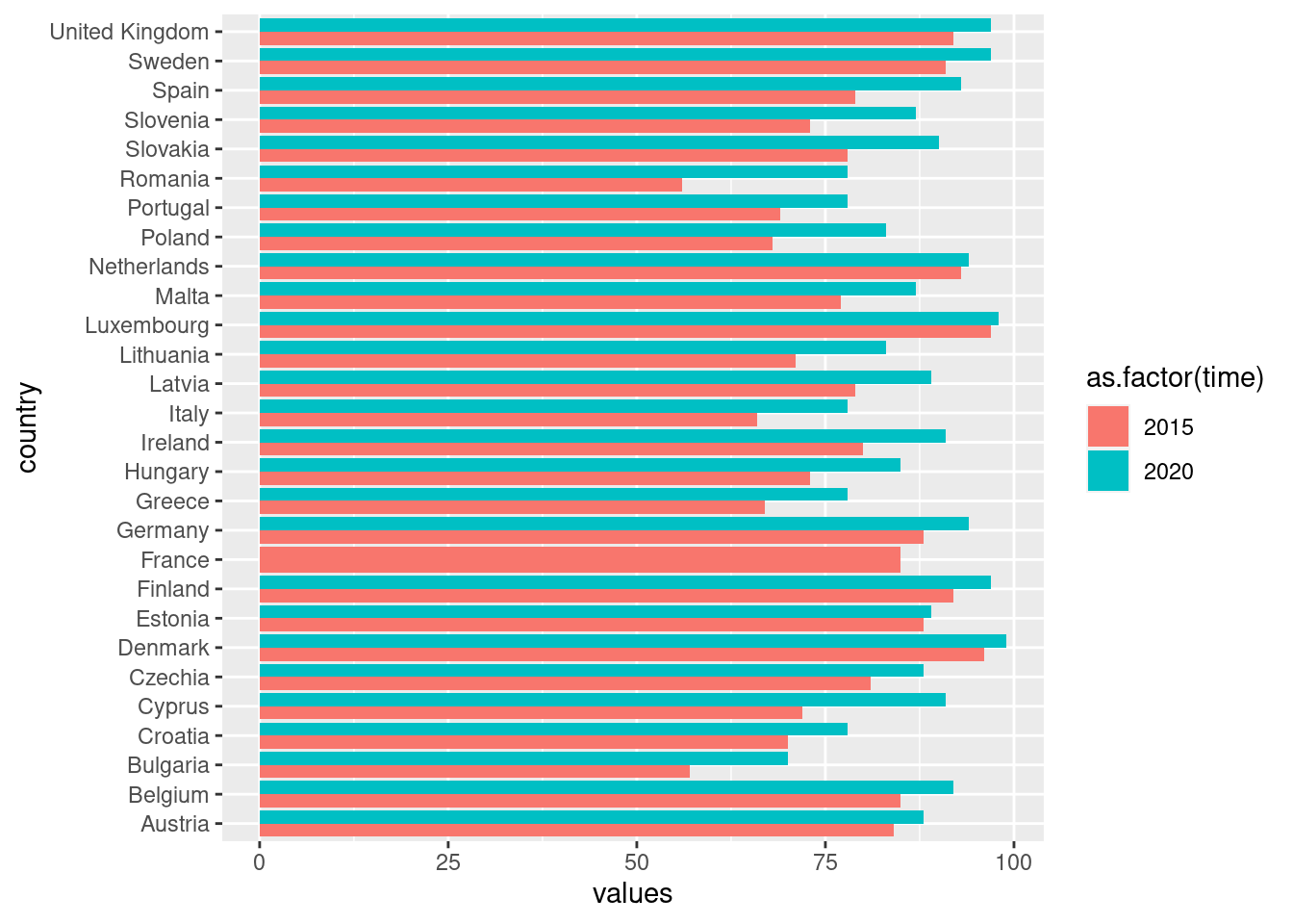

Let’s improve this. We will now transorm the data as follows:

eu_iuse <- iuse %>%
  inner_join(EU_countries, by = "geo") %>%
  filter(time %in% c(2015, 2020)) %>%
  filter(indic_is == 'I_IU3') %>%
  pivot_wider(id_cols = c(country, time),
              names_from = time,
              names_prefix = "y",
              values_from = values) %>%
  mutate(diff = y2020 - y2015)

The dataset now looks like:

eu_iuse

## # A tibble: 28 × 4
##    country  y2015 y2020  diff
##    <chr>    <dbl> <dbl> <dbl>
##  1 Austria     84    88     4
##  2 Belgium     85    92     7
##  3 Bulgaria    57    70    13
##  4 Cyprus      72    91    19
##  5 Czechia     81    88     7
##  6 Germany     88    94     6
##  7 Denmark     96    99     3
##  8 Estonia     88    89     1
##  9 Greece      67    78    11
## 10 Spain       79    93    14
## # … with 18 more rows

We have separate columns for the years 2008 and 2018, and we have created a new columns about the difference in percentages. Let’s plot it with points:

ggplot(eu_iuse) +
  geom_point(aes(x = country, y = y2015), color = "blue") +
  geom_point(aes(x = country, y = y2020), color = "red") +
  coord_flip() +
  labs(x = "Country", y = "% of individuals") +
  theme_bw() +
  theme(text = element_text(size = 16))

## Warning: Removed 1 rows containing missing values (geom_point).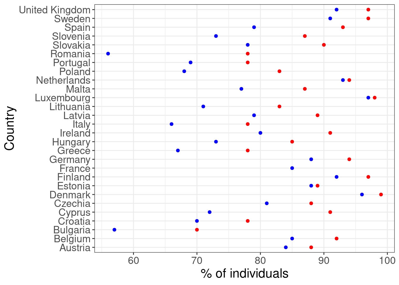

Everything is fine, but we can do even better. Ordering the data alphabetically per country name is not the best strategy. See this:

ggplot(eu_iuse) +
  geom_point(aes(x = reorder(country, y2015), y = y2020), color = "blue") +
  geom_point(aes(x = reorder(country, y2015), y = y2020), color = "red") +
  coord_flip() +
  labs(x = "Country", y = "% of individuals") +
  theme_bw() +
  theme(text = element_text(size = 16))

## Warning: Removed 1 rows containing missing values (geom_point).

## Warning: Removed 1 rows containing missing values (geom_point).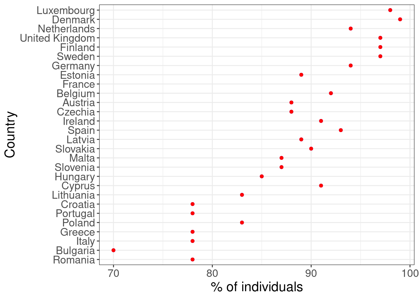

We have now the same data, the same plot, but ordering is based on values of the year 2008 (blue points). So we can clearly see the differences between Sweden (top) and Romania (bottom).

Another option would be ordering along the 2018 year (red points):

ggplot(eu_iuse) +
  geom_point(aes(x = reorder(country, y2020), y = y2015), color = "blue") +
  geom_point(aes(x = reorder(country, y2020), y = y2015), color = "red") +
  coord_flip() +
  labs(x = "Country", y = "% of individuals") +
  theme_bw() +
  theme(text = element_text(size = 16))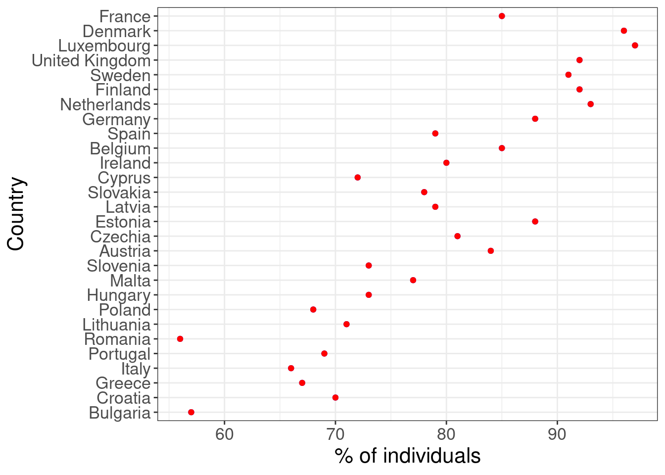

Both ways are correct and nice. Selection between them depends on the story we want to convey.

A third option would also be to order based of the distance covered between years 2008 and 2018, so using the diff column:

ggplot(eu_iuse) +
  geom_point(aes(x = reorder(country, diff), y = y2020), color = "blue") +
  geom_point(aes(x = reorder(country, diff), y = y2020), color = "red") +
  coord_flip() +
  labs(x = "Country", y = "% of individuals") +
  theme_bw() +
  theme(text = element_text(size = 16))

## Warning: Removed 1 rows containing missing values (geom_point).

## Warning: Removed 1 rows containing missing values (geom_point).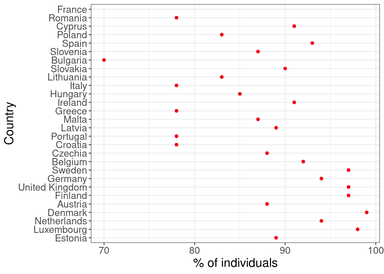

8.2 Annual Inflation

In this section we will discuss the annual inflation data in EU. These data can be retrived easily fron the tec00118 dataset:

tec00118 <- get_eurostat("tec00118", 
                         stringsAsFactors = FALSE, 
                         time_format = "num")

We will define one year we are interested in, for example 2019:

YR <- 2019

Again, as in other cases, we can create the auxilary EA_countries and EU_countries tables:

EA_countries <- ea_countries %>% 
  select(geo = code, Country = name)

EU_countries <- eu_countries %>% 
  select(geo = code, Country = name)

We need also the corresponding values of the EU average (EU28) and Euro Area countries (EA):

hicp_EU <- tec00118 %>% 
  filter(time == YR) %>% 
  filter(geo == 'EU28') %>%
  pull(values)
hicp_EA <- tec00118 %>% 
  filter(time == YR) %>% 
  filter(geo == 'EA') %>%
  pull(values)

A nice and quick way to compare values of inflation in EU28 countries:

tec00118 %>%
  filter(time == YR) %>%
  inner_join(EU_countries) %>% 
  ggbarplot(x = "Country", 
            y = "values",
            fill = "darkorange1",
            color = NA, 
            sort.val = "asc",
            orientation = "horizontal"
  ) +
  labs(x = "", 
       y = "HICP", 
       title = "Harmonised Index of Consumer Prices",
       subtitle = "Annual average rate of change of EU28 countries during 2019",
       caption = "Source: Eurostat tec00118") +
  theme_cleveland()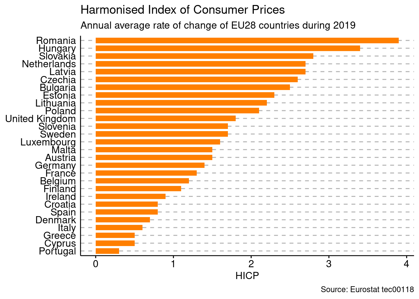

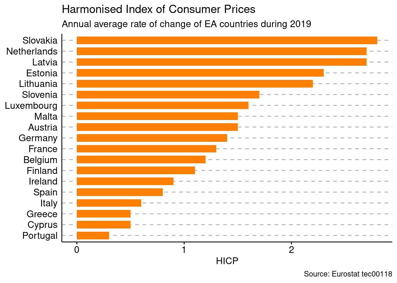
We can have a similar plot with only the Euro Area countries:

tec00118 %>%
  filter(time == YR) %>%
  inner_join(EA_countries) %>% 
  ggbarplot(x = "Country", 
            y = "values",
            fill = "darkorange1",
            color = NA, 
            sort.val = "asc",
            orientation = "horizontal"
  ) +
  labs(x = "", 
       y = "HICP", 
       title = "Harmonised Index of Consumer Prices",
       subtitle = "Annual average rate of change of EA countries during 2019",
       caption = "Source: Eurostat tec00118") +
  theme_cleveland()